Tracking as Online Decision-Making:
Learning a Policy from Streaming Videos with Reinforcement Learning
Abstract
We formulate tracking as an online decision-making process, where a tracking agent must follow an object despite ambiguous image frames and a limited computational budget. Crucially, the agent must decide where to look in the upcoming frames, when to reinitialize because it believes the target has been lost, and when to update its appearance model for the tracked object. Such decisions are typically made heuristically. Instead, we propose to learn an optimal decision-making policy by formulating tracking as a partially observable decision-making process (POMDP). We learn policies with deep reinforcement learning algorithms that need supervision (a reward signal) only when the track has gone awry. We demonstrate that sparse rewards allow us to quickly train on massive datasets, several orders of magnitude more than past work. Interestingly, by treating the data source of Internet videos as unlimited streams, we both learn and evaluate our trackers in a single, unified computational stream.
1 Introduction
Object tracking is one of the basic computational building blocks of video analysis, relevant for tasks such as general scene understanding and perception-for-robotics. A particularly popular formalism is that of model-free tracking, where a tracker is provided with a bounding-box initialization of an unknown object. Much of the recent state-of-the-art advances make heavy use of machine learning [25, 60, 43, 62, 21], often producing impressive results by improving core components such as appearance descriptors or motion modeling.
Challenges: We see two significant challenges that limit further progress in model-free tracking. First, the limited quantity of annotated video data impedes both training and evaluation. While image datasets involve millions of images for training and testing, tracking datasets have hundreds of videos. Lack of data seems to arise from the difficulty of annotating videos, as opposed to images. Second, as vision (re)-integrates with robotics, video processing must be done in an online, streaming fashion. In terms of tracking, this requires a tracker to make on-the-fly decisions such as when to re-initialize itself [57, 17, 33, 52, 22] or update its appearance model (the so-called template-update problem [60, 22]). Such decisions are known to be crucial in terms of final performance, but are typically hand-designed rather than learned.
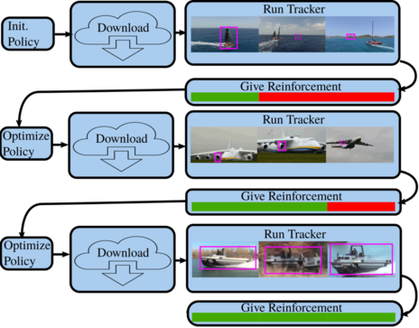
Contribution 1 (interactive video processing): We show that reinforcement learning (RL) can be used to address both challenges in distinct ways. In terms of data, rather than requiring videos to be labeled with detailed bounding-boxes at each frame, we interactively train trackers with far more limited supervision (specifying binary rewards/penalties only when a tracker fails). This allows us to train on massive video datasets that are larger than prior work. Interestingly, RL also naturally lends itself to streaming “open-world” evaluation: when running a tracker on a never-before-seen video, the video can be used for both evaluation of the current tracker and for training (or refining) the tracker for future use (Fig. 1). This streaming evaluation allows us to train and evaluate models in an integrated fashion seamlessly. For completeness, we also evaluate our learned models on standard tracking benchmarks.
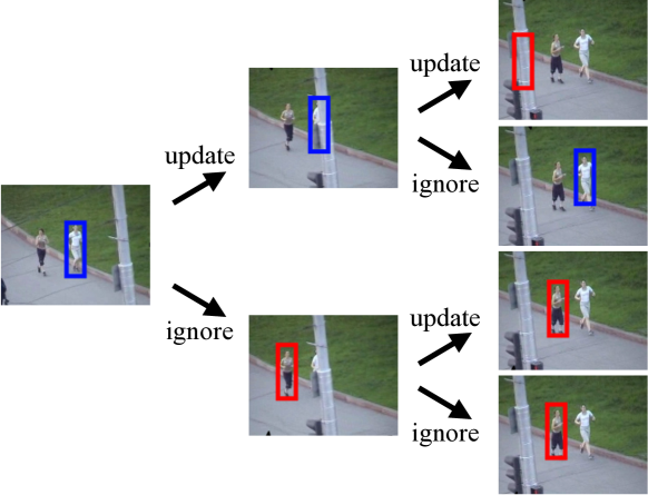
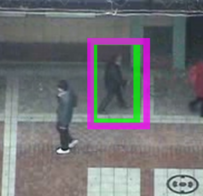
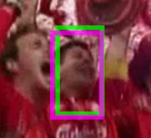
Contribution 2 (tracking as decision-making): In terms of tracking, we model the tracker itself as an active agent that must make online decisions to maximize its reward, which is (as above) the correctness of a track. Decisions ultimately specify where to devote finite computational resources at any point of time: should the agent process only a limited region around the currently predicted location (e.g.,“track”), or should it globally search over the entire frame (“reinitialize”)? Should the agent use the predicted image region to update its appearance model for the object being tracked (“update”), or should it be “ignored”? Such decisions are notoriously complicated when image evidence is ambiguous (due to say, partial occlusions): the agent may continue tracking an object but perhaps decide not to update its model of the object’s appearance. Rather than defining these decisions heuristically, we will ultimately use data-driven techniques to learn good policies for active decision-making (Fig. 2).
Contribution 3 (deep POMDPs): We learn tracker decision policies using reinforcement learning. Much recent work in this space assumes a Markov Decision Process (MDP), where the agent observes the true state of the world [37, 62], which is the true (possibly 3D) location and unoccluded appearance of the object being tracked. In contrast, our tracker only assumes that it receives partial image observations about the world state. The resulting partially-observable MDP (POMDP) violates Markov independence assumptions: actions depend on the entire history of observations rather than just the current one [20, 47]. As in [16, 23], we account for this partial observability by maintaining a memory that captures beliefs about the world, which we update over time (Sec. 3). In our case, beliefs capture object location and appearance, and action policies specify how and when to update those beliefs (e.g., how and when should the tracker update its appearance model) (Sec. 4). However, policy-learning is notoriously challenging because actions can have long-term effects on future beliefs. To efficiently learn policies, we introduce frame-based heuristics that provide strong clues as to the long-term effects of taking a particular action (Sec. 5).
2 Related Work
Tracking datasets:
Several established benchmarks exist for evaluating trackers [61, 25]. Interestingly, there is evidence to suggest that many methods tend to overfit due to aggressive tuning [43]. Withholding test data annotation and providing an evaluation server addresses this to some extent [29, 46]. Alternatively, we propose to evaluate on an open-world stream of Internet videos, making over-fitting impossible by design. It is well-known that algorithms trained on “closed-world” datasets (say, with centered objects against clean backgrounds [42, 4]) are difficult to generalize to “in-the-wild” footage [54]. We invite the reader to compare our videos in the supplementary material to contemporary video benchmarks for tracking.
Interactive tracking:
Several works have explored interactive methods that use trackers to help annotate data. The computer first proposes a track. Then a human corrects major errors and retrains the tracker using the corrections [9, 2, 56]. Our approach is closely inspired by such active learning formalisms but differs in that we make use of minimal supervision in the form of a binary reward (rather than a bounding box annotation).
Learning-to-track:
Many tracking benchmarks tend to focus on short-term tracking ( frames per video) [61, 25]. In this setting, a central issue appears to be modeling the appearance of the target. Methods that use deep features learned from large-scale training data perform particularly well [57, 58, 32, 30, 39]. Our focus on tracking over longer time frames poses additional challenges - namely, how to reinitialize after cuts, occlusions and failures, despite changes in target appearance [15, 60]. Several trackers address these challenges with hand-designed policies for model updating and reinitialization - TLD [22], ALIAN [44] and SPL [52] explicitly do so in the context of long-term tracking. On the other hand, our method takes a data-driven approach and learns policies for model-updating and reinitialization. Interestingly, such an “end-to-end” learning philosophy is often embraced by the multi-object tracking community, where strategies for online reinitialization and data association are learned from data [26, 62, 31]. Most related to us are [62], who use an MDP for multi-object tracking, and [23], who use RL for single target tracking. Both works use heuristics to reduce policy learning to a supervised learning task, avoiding the need to reason about rewards in the far future. The robotics community has developed techniques to accelerate RL using human demonstrations [28], interactive feedback [24, 53], and hand-designed heuristics [7]. Using heuristic functions for initialization [7, 24], our experimental results show that explicit Q-learning outperforms supervised reductions because it can learn to capture long-term effects of taking particular actions.
Real-time tracking through attention:
An interesting (but perhaps unsurprising) phenomenon is that better trackers tend to be slower [25]. Indeed, on the VOT benchmark, most recent trackers do not run in real time. Generally, trackers that search locally [50, 55] run faster than those that search globally [52, 33, 18]. To optimize visual recognition efficiency, one can learn a policy to guide selective search or attention. Inspired by recent work which finds a policy for selective search using RL [21, 36, 41, 11, 19, 3, 34], we also learn a policy that decides whether to track (i.e., search positions near the previous estimate) or reinitialize (i.e., search globally over the entire image). But in contrast to this prior work, we additionally learn a policy to decide when to update a tracker’s appearance model. To ensure that our tracker operates with a fixed computational budget, we implement reinitialization by searching over a random subset of positions (equal in number to those examined by track).
| Dataset | # Videos | # Frames | Annotations | Type |
|---|---|---|---|---|
| OTB-2013 [61] | 50 | 29,134 | 29,134 | AABB |
| PTB [51] | 50 | 21,551 | 21,551 | AABB |
| VOT-2016 [25] | 60 | 21,455 | 21,455 | RBB |
| ALOV++ [49] | 315 | 151,657 | 30,331 | AABB |
| NUS-PRO [29] | 365 | 135,310 | 135,310 | AABB |
| Ours | 16,384 | 10,895,762 | 108,957 | Binary |
3 POMDP Tracking
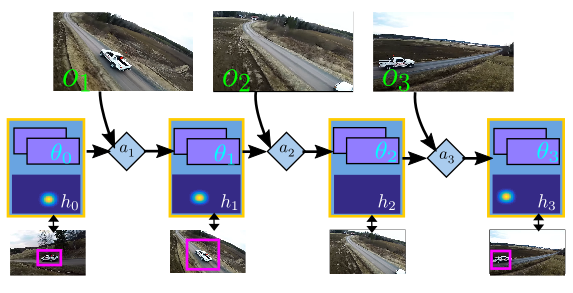
We now describe our POMDP tracker, using standard notation where possible [47]. For our purposes, a POMDP is defined by a tuple of states (): At each frame , the world state generates a noisy observation that is mapped by an agent into an action , which in turn generates a reward.
In our case, the state captures the true location and appearance of the object being tracked in frame . To help build intuition, one can think of the location as 2D pixel coordinates and appearance as a 2D visual template. Instead of directly observing this world state, the tracking agent maintains a belief over world states, written as
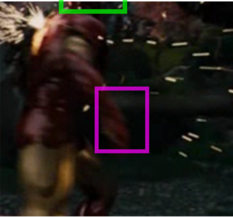
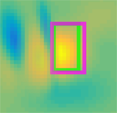
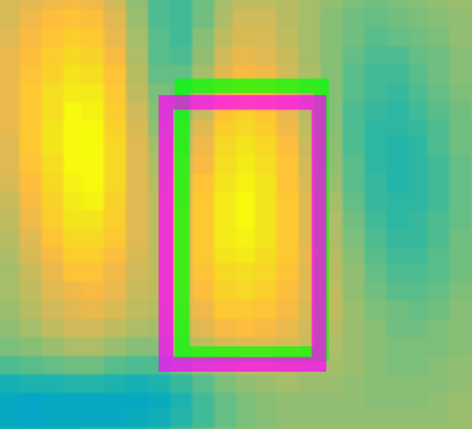
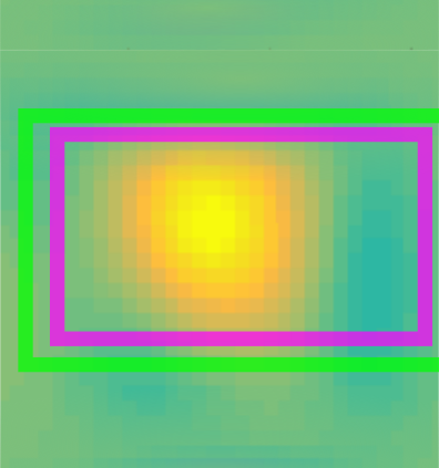
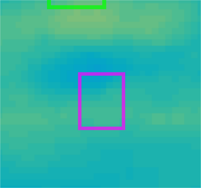
where is a distribution over appearances (we use a point-mass distribution encoded by a single filter defined on convolutional features), and is a distribution over pixel positions (encoded as a spatial heatmap of size ). Given the previous belief and current observed video frame , the tracking agent updates its beliefs about the current frame . Crucially, tracker actions specify how to update its beliefs, that is, whether to update the appearance model and whether to reinitialize by disregarding previous heatmaps. From this perspective, our POMDP tracker is a memory-based agent that learns a policy for when and how to update its own memory (Fig. 3).
Specifically, beliefs are updated as follows:
| (3) | ||||
| (6) |
where . Object heatmaps are updated by running the current appearance model on image regions near the target location previously predicted using (“tracking”). Alternatively, if the agent believes it has lost track, it may globally evaluate its appearance model (“reinit”). The agent may then decide to “update” its appearance model using the currently-predicted target location, or it may leave its appearance model unchanged. In our framework, the tracking, reinitialization, and appearance-update modules can be treated as black boxes given the above functional form. We will discuss particular implementations shortly, but first, we focus on the heart of our RL approach: a principled framework for learning to take appropriate actions. To do so, we begin by reviewing standard approaches for decision-making.
Online heuristics: The simplest approach to picking actions might be to pre-define heuristics functions which estimate the correct action. For example, many trackers reinitialize whenever the maximum confidence of the heatmap is below a threshold. Let us summarize the information available to the tracker at frame as a “state” , which includes the previous belief (the previous heatmap and appearance model) and current image observation .
| (7) |
Offline heuristics: A generalization of the above is to use offline training data to build better heuristics. Crucially, one can now make use of ground-truth training annotations as well as future frames to better gauge the impact of possible actions. We can write this knowledge as the true world state . For example, a natural heuristic may be to reinitialize whenever the predicted object location does not overlap the ground-truth position for that frame. Similarly, one may update appearance whenever doing so improves the confidence of ground-truth object locations across future frames:
| (8) |
Crucially, these heuristics cannot be applied at test time because ground truth is not known! However, they can generate per-frame target action labels on training data, effectively reducing policy learning to a standard supervised-learning problem. Though offline heuristics appear to be a simple and intuitive approach to policy learning, we have not seen them widely applied for learning tracker action policies.
Q-functions: Offline heuristics can be improved by unrolling them forward in time: the benefit of a putative action can be better modeled by applying that action, processing the next frame, and using the heuristic to score the “goodness” of possible actions in that next frame. This intuition is formalized through the well-known Bellman equations that recursively define Q-functions to return a goodness score (the expected future reward) for each putative action :
| (9) |
where includes both the tracker belief state and image observation, and is the reward associated with the reporting the estimated object heatmap . We let for a correct prediction and otherwise. Finally, is a discount factor that trades off immediate vs. future per-frame rewards. Given a tracker state and image observation , the optimal action to take is readily computed from the Q-function:
Q-learning: Traditionally, Q-functions are iteratively learned with Q-learning [47]:
| (10) | ||||
where is a learning rate. To handle continuous belief states, we approximate the Q-function with a CNNs:
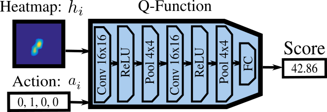
that processes states and binary actions to return a scalar value capturing the expected future reward for taking that action. Recall that a state encodes a heatmap and an appearance model from previous frames and an image observation from the current frame.
4 Interactive Training and Evaluation

In this section, we describe our procedure for interactively learning CNN parameters (that encode tracker action policies) from streaming video datasets. To do so, we gradually build up a database of experience replay memories [1, 37], which are a collection of state-action-reward-nextstate tuples . Q-learning reduces policy learning to a supervised regression problem by unrolling the current policy one step forward in time. This unrolling results in the standard Q-loss function [37]:
| (11) |
Gradient descent on the above objective is performed as follows: given a training sample , first perform a forward pass to compute the current estimate and the target: . Then backpropagate through the weights to reduce .
The complete training algorithm is written in Alg. 1 and illustrated in Fig. 1. We choose random videos from the Internet by sampling phrases using WordNet [35]. Given the sampled phrase and video, an annotator provides an initialization bounding box and begins running the existing tracker. After tracking, the annotator marks those frames (in strides of 50) where the tracker was incorrect using a standard 50% intersection-over-union threshold. Such binary annotation (“correct” or “failed”) requires far less time per frame than bounding-box annotation: we design a real-time interface that simply requires a user to depress a button during tracker failures. By playing back videos at a (user-selected) sped-up frame rate, users annotate 1200 frames per minute on average (versus 34 for bounding boxes). Annotating our entire dataset of 10 million frames (Table 1) requires a little under two-days of labor, versus the months required for equivalent bounding-box annotation. After running our tracker and interactively marking failures, we use the annotation as a reward signal to update the policy parameters for the next video. Thus each video is used to both evaluate the current tracker and train it for future videos.
5 Implementation
In this section, we discuss several implementation details. We begin with a detailed overview of our tracker’s test time pipeline. The implementation details for the TRACK, REINIT, UPDATE, and Q-functions follow. Finally, we describe the offline heuristics used at train time.
Overview of p-tracker’s pipeline:
TRACK/REINIT functions:
Our TRACK function (Eq. 6) takes as input the previous heatmap , appearance model , and image observation , and produces a new heatmap for the current frame. We experiment with implementing TRACK using either of two state-of-the-art fully-convolutional trackers: FCNT [57] or CCOT [13]. We refer to the reader to the original works for precise implementation details, but summarize them here: TRACK crops the current image to a region of interest (ROI) around the most likely object location from the previous frame (the argmax of ). This ROI is resized to a canonical image size (e.g., ) and processed with a CNN (VGG [48]) to produce a convolutional feature map. The object appearance model is represented as a filter on this feature map, allowing one to compute a new heatmap with a convolution. When the tracker decides that it has lost track, the REINIT model simply processes a random ROI. In general, we find CCOT to outperform FCNT (consistent with the reported literature) and so focus on the former in our experiments, though we include diagnostic results with both trackers (to illustrate the generality of our approach).
UPDATE function: We update the current filter using positive and negative patches extracted from the current frame . We extract a positive patch from the maximal location in the reported heatmap , and extract negative patches from adjacent regions with less than 30% overlap. We update following the default scheme in the underlying tracker: for FCNT, is a two-layer convolutional template that is updated with a fixed number of gradient descent iterations (10). For CCOT, is a multi-resolution set of convolutional templates that is fit through conjugate gradients.
Q-function CNN: Recall that our Q-functions process a tracker state and a candidate action , to return a scalar representing the expected future reward of taking that action (Fig. 5 and Eq. 11). In practice, we define two separate Q-functions for our two binary decisions (TRACK/REINIT and UPDATE/IGNORE). To plug into standard learning approaches, we formally define a single function as the sum of the two functions, implying that the optimal decisions can be computed independently for each. We found it sufficed to condition on the heatmap and implemented each function as a CNN, where the first two hidden layers are shared across the two functions. Each shared hidden layer consists of convolution followed by ReLU and max pooling. For each decision, an independent fully-connected layer ultimately predicts the expected future reward. When training the Q-function using experience-replay, we use , a learning rate of 1e-4, a momentum of .9 and 1e-8 weight decay.
Offline heuristics: Deep q-learning is known to be unstable, and we found good initialization was important for reliable convergence. We initialize the Q-functions in Eq. 11 (which specify the goodness of particular actions) with the offline heuristics from Eq. 8. Specifically, the heuristic action has a goodness of 1 (scaled by future discount rewards), while other actions have a goodness of 0:
| (12) |
where denotes the identity function. In practice, we found it useful to minimize a weighted average of the true loss in Eq. 11 and a supervised loss , an approach related to heuristically-guided Q-learning [21, 8]. Defining a heuristic for TRACK vs REINIT is straightforward: should TRACK whenever the peak of the reported heatmap overlaps the ground-truth object on frame . Defining a heuristic for UPDATE vs IGNORE is more subtle. Intuitively, should UPDATE appearance with frame whenever doing so improves the confidence of future ground-truth object locations in that video. To operationalize this, we update the current appearance model on samples from frame and compute , the number of future frames where the updated appearance increases confidence of ground-truth locations (and similarly , the number of frames where the update decreases confidence of track errors). We set to update when , where N is the total number of future frames.
6 Experiments
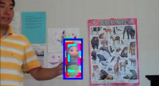
| Online Tracking Benchmark [61] | |||||
|---|---|---|---|---|---|
 |
 |
 |
 |
 |
 |
 |
 |
 |
 |
 |
 |
 p-track(ours)
FCNT
CCOT [13]
TCNN [38]
SSAT [40]
MLDF [59]
Staple [5]
DDC [25]
EBT [63]
SRBT [25]
STAPLEp [5]
DNT [10]
SSKCF [27]
SiamRN [6]
DeepSRDCF [12]
SHCT [14]
Evaluation metrics:
Following established protocols for long-term tracking [22, 52], we evaluate , where precision is the fraction of predicted locations that are correct and recall is the fraction of ground-truth locations that are correctly predicted. Because Internet videos vary widely in difficulty, we supplement averages with boxplots to better visualize performance skew. When evaluating results on standard benchmarks, we use the default evaluation criteria for that benchmark.
| Internet Videos | |||
|---|---|---|---|
|
Transform |
 |
 |
 |
|
SpaceX |
 |
 |
 |
|
SnowTank |
 |
 |
 |
|
JohnWick |
 |
 |
 |
F1-measure
6.1 Comparative Evaluation
Short-term benchmarks:
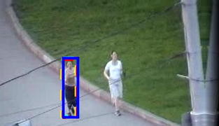
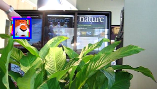
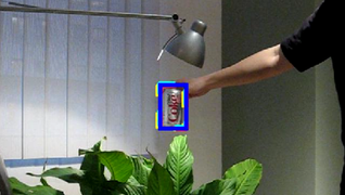
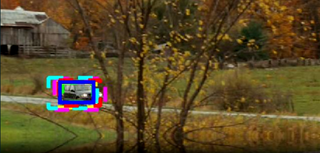
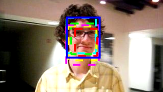
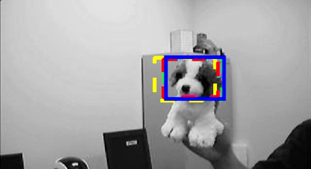
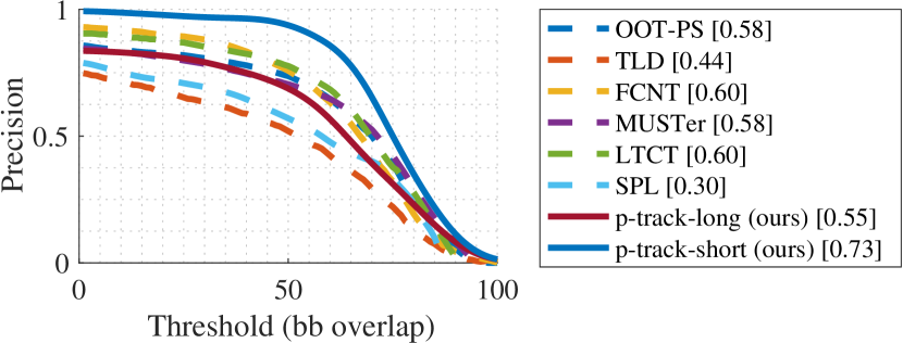
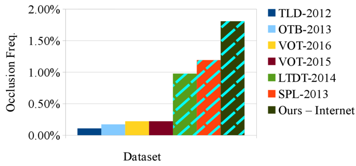
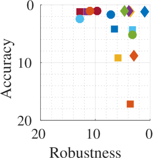
While our focus is long-term tracking, we begin by presenting results on existing benchmarks that tend to focus on the short-term setting – the Online Tracker Benchmark (OTB-2013) [61] and Visual Object Tracking Benchmark (VOT-2016) [25]. Our policy tracker (p-track-long), trained on Internet videos, performs competitively (Fig. 7), but tends to over-predict occlusions (which rarely occur in short-term videos, as shown in Fig. 8). Fortunately, we can learn dedicated policies for short-term tracking (p-track-short) by applying reinforcement learning (Alg. 1) on short-term training videos. For each test video in OTB-2013, we learn a policy using the 40 most dissimilar videos in VOT-2016 (and vice-versa). We define similarity between videos to be the correlation between the average (ground-truth) object image in RGB space. This ensures that, for example, we do not train using Tiger1 when testing on Tiger2. Even under this controlled scenario, p-track-short significantly outperforms prior work on both OTB-2013 (Figs. 6 and 7) and VOT-2016 (Fig. 9).
Long-term baselines:
For the long-term setting, we compare to two classic long-term trackers: TLD [22] and SPL [52]. Additionally, we also compare against short-term trackers with public code that we were able to adapt: FCNT [57], MUSTer [17], and LTCT [33]. Notably, all these baselines use hand-designed heuristics for deciding when to appearance update and reinitialize.
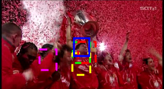
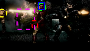
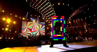
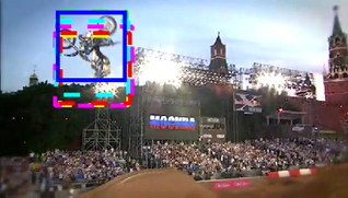
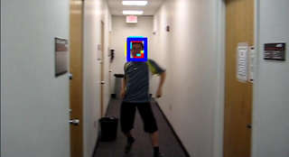
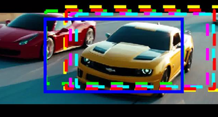
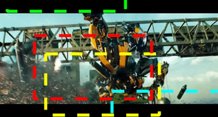
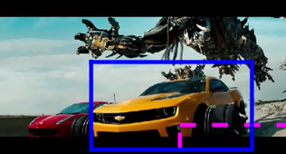
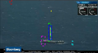
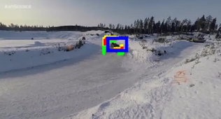
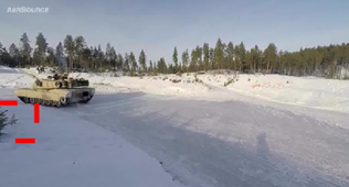
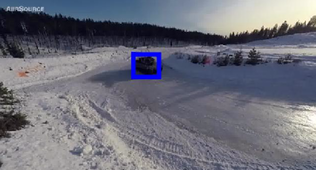
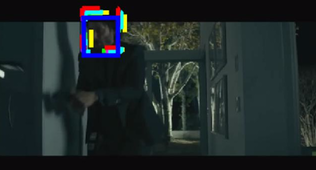
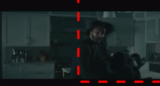
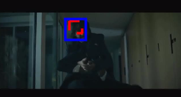
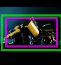
Long-term videos: Qualitatively speaking, long term videos from the internet are much more difficult than standard benchmarks (c.f. Fig 6 and Fig. 10). First, many standard benchmarks tend to contain videos that are easy for most modern tracking approaches, implying that a method’s rank is largely determined by performance on a small number of challenging videos. The easy videos focus on iconic [42, 4] views with slow motion and stable lighting conditions [29], featuring no cuts or long-term occlusions [15]. Internet videos are significantly more complex. One major reason is the presence of frequent cuts. We think that Internet videos with multiple cuts provide a valuable proxy for occlusions, particularly since they are a scalable data source. In theory, long-term trackers must be able to re-detect the target after an occlusion (or cut), but there is still much room for improvement. Also, many strange things happen in the wild world of Internet videos. For example, in Transform the car transforms into a robot, confusing all trackers (including ours). In SnowTank the tracker must contend with many distractors (tanks of different colors and type) and widely varying viewpoint and scale. Meanwhile, JohnWick contains poor illumination, fast motion, and numerous distractors.
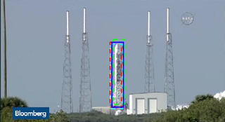
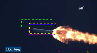
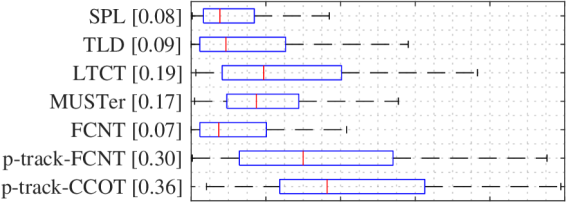
Long-term results: To evaluate results for “in-the-wild” long-term tracking, we define a new 16-video held-out test set of long-term Internet videos that is never used for training. Each of our test videos contains at least 5,000 frames, a common definition of “long-term” [52, 33, 17, 15]. We compare our method to various baselines in Fig. 11. Comparisons to FCNT [57] and CCOT [13] are particularly interesting since we can make use of their TRACK and UPDATE modules. While FCNT performs quite well in the short-term (Fig. 7), it performs poorly on long-term sequences (Fig. 11). However, by learning a policy for updating and reinitialization, we produce a state-of-the-art long-term tracker. We visualize the learned policy in Fig. 14.
6.2 System Diagnostics
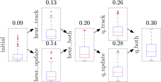
We now provide a diagnostic analysis of various components of our system. We begin by examining several alternative strategies for making sequential decisions (Fig. 12).
FCNT vs. CCOT:
We use FCNT for our ablative analysis; initializing p-track using CCOT’s more complex online heuristics proved difficult. However our final system uses only our proposed offline heuristics, so we can nonetheless train it using CCOT’s TRACK, REINIT, and UPDATE functions. In Fig. 11 we compare the final p-trackers built using FCNT’s functions against those built using CCOT’s functions. As consistent with prior work, we find that CCOT improves overall performance (from .30 to .36).
Online vs. offline heuristics:
We begin by analyzing the online heuristic actions of our baseline tracker, FCNT. FCNT updates an appearance model when the predicted heatmap location is above a threshold, and always tracks without reinitialization. This produces a F1 score of .09. Next, we use offline heuristics to learn the best action to take. These correspond to tracking when the predicted object location is correct, and updating if the appearance model trained on the new patch produces higher scores for ground-truth locations. We train a classifier to predict these actions using the current heatmap. When this offline trained classifier is run at test time, F1 improves to .13 with the track heuristic alone, .14 with the update heuristic alone, and .20 if both are used.
Q-learning:
Finally, we use Q-learning to refine our heuristics (Eq. 11), noticeably improving the F1 score to .30. Learning the appearance update action seems to have the most significant effect on performance, producing an F1 score of .28 by itself. During partial occlusions, the tracker learns to delicately balance between appearance update and drift while accepting a few failures to avoid the cost and risk of reinitialization. Overall, the learned policy dramatically outperforms the default online heuristics, tripling the F1 score from 9% to 30%!

Training iterations:
In theory, our tracker can be interactively trained on a never-ending stream. However, in our experiments, Q-learning appeared to converge after seeing between 8,000 and 12,000 videos. Thus, we choose to stop training after seeing 16,000 videos. In Fig. 13, we plot performance versus training iteration.
Computation:
As mentioned previously, comparatively slower trackers typically perform better [25]. On a Tesla K40 GPU, our tracker runs at approximately 10 fps. While computationally similar to [57], we add the ability to recover from tracking failures by reinitializing through detection. To do so, we learn an attention policy that efficiently balances tracking versus reinitialization. Tracking is fast because only a small region of interest (ROI) need be searched. Rather than searching over the whole image during reinitialization, we select a random ROI (which ensures that our trackers operate at a fixed frame rate). In practice, we find that target is typically found in frames.
| (a) Track & Update | (b) Track Only | (c) Track Only | (d) Reinit |
|---|---|---|---|
 |
 |
 |
 |
 |
 |
 |
 |
| Ground Truth | Tracker’s Localization |
Conclusions:
We formulate tracking as a sequential decision-making problem, where a tracker must update its beliefs about the target, given noisy observations and a limited computational budget. While such decisions are typically made heuristically, we bring to bear tools from POMDPs and reinforcement learning to learn decision-making strategies in a data-driven way. Our framework allows trackers to learn action policies appropriate for different scenarios, including short-term and long-term tracking. One practical observation is that offline heuristics are an effective and efficient way to learn tracking policies, both by themselves and as a regularizer for Q-learning. Finally, we demonstrate that reinforcement learning can be used to leverage massive training datasets, which will likely be needed for further progress in data-driven tracking.
References
- [1] S. Adam, L. Busoniu, and R. Babuska. Experience replay for real-time reinforcement learning control. IEEE Transactions on Systems, Man, and Cybernetics, 42(2):201–212, 2012.
- [2] A. Agarwala, A. Hertzmann, D. H. Salesin, and S. M. Seitz. Keyframe-based tracking for rotoscoping and animation. ACM Transactions on Graphics (ToG), 23(3):584–591, 2004.
- [3] L. Bazzani, N. de Freitas, and J.-A. Ting. Learning attentional mechanisms for simultaneous object tracking and recognition with deep networks. In NIPS 2010 Deep Learning and Unsupervised Feature Learning Workshop, volume 32, 2010.
- [4] T. Berg and A. C. Berg. Finding iconic images. CVPR, 2009.
- [5] L. Bertinetto, J. Valmadre, S. Golodetz, O. Miksik, and P. H. Torr. Staple: Complementary learners for real-time tracking. In Proceedings of the IEEE Conference on Computer Vision and Pattern Recognition, pages 1401–1409, 2016.
- [6] L. Bertinetto, J. Valmadre, J. F. Henriques, A. Vedaldi, and P. H. Torr. Fully-convolutional siamese networks for object tracking. In European Conference on Computer Vision, pages 850–865. Springer, 2016.
- [7] R. A. Bianchi, C. H. Ribeiro, and A. H. Costa. Accelerating autonomous learning by using heuristic selection of actions. Journal of Heuristics, 14(2):135–168, 2008.
- [8] R. A. Bianchi, C. H. Ribeiro, and A. H. R. Costa. Heuristically accelerated reinforcement learning: Theoretical and experimental results. ECAI, pages 169–174, 2012.
- [9] A. Buchanan and A. Fitzgibbon. Interactive feature tracking using kd trees and dynamic programming. In CVPR, volume 1, pages 626–633, 2006.
- [10] Z. Chi, H. Li, H. Lu, and M.-H. Yang. Dual deep network for visual tracking. IEEE Transactions on Image Processing, 26(4):2005–2015, 2017.
- [11] L. Chukoskie, J. Snider, M. C. Mozer, R. J. Krauzlis, and T. J. Sejnowski. Learning where to look for a hidden target. Proceedings of the National Academy of Sciences, 110(Supplement 2):10438–10445, 2013.
- [12] M. Danelljan, G. Hager, F. Shahbaz Khan, and M. Felsberg. Learning spatially regularized correlation filters for visual tracking. In Proceedings of the IEEE International Conference on Computer Vision, pages 4310–4318, 2015.
- [13] M. Danelljan, A. Robinson, F. S. Khan, and M. Felsberg. Beyond correlation filters: Learning continuous convolution operators for visual tracking. In European Conference on Computer Vision, pages 472–488. Springer, 2016.
- [14] D. Du, H. Qi, W. Li, L. Wen, Q. Huang, and S. Lyu. Online deformable object tracking based on structure-aware hyper-graph. IEEE Transactions on Image Processing, 25(8):3572–3584, 2016.
- [15] M. Edoardo Maresca and A. Petrosino. The matrioska tracking algorithm on LTDT2014 dataset. CVPR workshop on LTDT, 2014.
- [16] M. Hausknecht and P. Stone. Deep recurrent q-learning for partially observable MDPs. arXiv:1507.06527, 2015.
- [17] Z. Hong, Z. Chen, C. Wang, X. Mei, D. Prokhorov, and D. Tao. Multi-store tracker (muster): a cognitive psychology inspired approach to object tracking. CVPR, pages 749–758, 2015.
- [18] Y. Hua, K. Alahari, and C. Schmid. Online object tracking with proposal selection. ICCV, pages 3092–3100, 2015.
- [19] M. Jiang, X. Boix, G. Roig, J. Xu, L. Van Gool, and Q. Zhao. Learning to predict sequences of human visual fixations. IEEE transactions on neural networks and learning systems, 27(6):1241–1252, 2016.
- [20] L. P. Kaelbling, M. L. Littman, and A. R. Cassandra. Planning and acting in partially observable stochastic domains. Artificial intelligence, 101(1):99–134, 1998.
- [21] S. E. Kahou, V. Michalski, and R. Memisevic. RATM: Recurrent attentive tracking model. CVPR, 2016.
- [22] Z. Kalal, K. Mikolajczyk, and J. Matas. Tracking-learning-detection. TPAMI, 34(7):1409–1422, 2012.
- [23] S. Khim, S. Hong, Y. Kim, and P. kyu Rhee. Adaptive visual tracking using the prioritized q-learning algorithm: Mdp-based parameter learning approach. Image and Vision Computing, 32(12):1090–1101, 2014.
- [24] W. B. Knox and P. Stone. Augmenting reinforcement learning with human feedback. In ICML 2011 Workshop on New Developments in Imitation Learning (July 2011), volume 855, 2011.
- [25] M. Kristan, A. Leonardis, J. Matas, M. Felsberg, R. Pflugfelder, L. Čehovin, T. Vojir, G. Häger, A. Lukežič, and G. Fernandez. The visual object tracking vot2016 challenge results. Springer, Oct 2016.
- [26] L. Leal-Taixé, A. Milan, I. Reid, S. Roth, and K. Schindler. MOTchallenge 2015: Towards a benchmark for multi-target tracking. arXiv:1504.01942, 2015.
- [27] J.-Y. Lee and W. Yu. Visual tracking by partition-based histogram backprojection and maximum support criteria. In Robotics and Biomimetics (ROBIO), 2011 IEEE International Conference on, pages 2860–2865. IEEE, 2011.
- [28] L. A. León, A. C. Tenorio, and E. F. Morales. Human interaction for effective reinforcement learning. In European Conf. Mach. Learning and Principles and Practice of Knowledge Discovery in Databases (ECMLPKDD 2013), 2013.
- [29] A. Li, M. Lin, Y. Wu, M.-H. Yang, and S. Yan. NUS-PRO: A new visual tracking challenge. 2015.
- [30] H. Li, Y. Li, F. Porikli, et al. Deeptrack: Learning discriminative feature representations by convolutional neural networks for visual tracking. BMVC, 1(2):3, 2014.
- [31] Y. Li, C. Huang, and R. Nevatia. Learning to associate: Hybridboosted multi-target tracker for crowded scene. CVPR, pages 2953–2960, 2009.
- [32] C. Ma, J.-B. Huang, X. Yang, and M.-H. Yang. Hierarchical convolutional features for visual tracking. ICCV, pages 3074–3082, 2015.
- [33] C. Ma, X. Yang, C. Zhang, and M.-H. Yang. Long-term correlation tracking. CVPR, pages 5388–5396, 2015.
- [34] S. Mathe, A. Pirinen, and C. Sminchisescu. Reinforcement learning for visual object detection. In Proceedings of the IEEE Conference on Computer Vision and Pattern Recognition, pages 2894–2902, 2016.
- [35] G. A. Miller. Wordnet: a lexical database for english. Communications of the ACM, 38(11):39–41, 1995.
- [36] V. Mnih, N. Heess, A. Graves, et al. Recurrent models of visual attention. NIPS, pages 2204–2212, 2014.
- [37] V. Mnih, K. Kavukcuoglu, D. Silver, A. A. Rusu, J. Veness, M. G. Bellemare, A. Graves, M. Riedmiller, A. K. Fidjeland, G. Ostrovski, et al. Human-level control through deep reinforcement learning. Nature, 518(7540):529–533, 2015.
- [38] H. Nam, M. Baek, and B. Han. Modeling and propagating cnns in a tree structure for visual tracking. arXiv preprint arXiv:1608.07242, 2016.
- [39] H. Nam and B. Han. Learning Multi Domain Convolutional Neural Networks for Visual Tracking. arXiv:1510.07945, 2015.
- [40] H. Nam and B. Han. Learning multi-domain convolutional neural networks for visual tracking. In Proceedings of the IEEE Conference on Computer Vision and Pattern Recognition, pages 4293–4302, 2016.
- [41] L. Paletta, G. Fritz, and C. Seifert. Q-learning of sequential attention for visual object recognition from informative local descriptors. ICML, pages 649–656, 2005.
- [42] S. Palmer, E. Rosch, and P. Chase. Canonical perspective and the perception of objects. Attention and performance, 1(4), 1981.
- [43] Y. Pang and H. Ling. Finding the Best from the Second Bests - Inhibiting Subjective Bias in Evaluation of Visual Tracking Algorithms. ICCV, pages 2784–2791, dec 2013.
- [44] F. Pernici and A. Del Bimbo. Object tracking by oversampling local features. TPAMI, 36(12):2538–2551, 2014.
- [45] J. Rumbaugh, I. Jacobson, and G. Booch. Unified modeling language reference manual, the. Pearson Higher Education, 2004.
- [46] O. Russakovsky, J. Deng, H. Su, J. Krause, S. Satheesh, S. Ma, Z. Huang, A. Karpathy, A. Khosla, M. Bernstein, A. C. Berg, and L. Fei-Fei. ImageNet Large Scale Visual Recognition Challenge. IJCV, 115(3):211–252, 2015.
- [47] S. J. Russell, P. Norvig, J. F. Canny, J. M. Malik, and D. D. Edwards. Artificial intelligence: a modern approach. Prentice Hall, 2003.
- [48] K. Simonyan and A. Zisserman. Very deep convolutional networks for large-scale image recognition. CoRR, abs/1409.1556, 2014.
- [49] A. W. Smeulders, D. M. Chu, R. Cucchiara, S. Calderara, A. Dehghan, and M. Shah. Visual tracking: An experimental survey. TPAMI, 36(7):1442–1468, 2014.
- [50] A. Solis Montero, J. Lang, and R. Laganiere. Scalable kernel correlation filter with sparse feature integration. ICCV Workshops, December 2015.
- [51] S. Song and J. Xiao. Tracking revisited using RGBD camera: Unified benchmark and baselines. ICCV, pages 233–240, 2013.
- [52] J. Supancic and D. Ramanan. Self-paced learning for long-term tracking. CVPR, pages 2379–2386, 2013.
- [53] A. L. Thomaz, G. Hoffman, and C. Breazeal. Real-time interactive reinforcement learning for robots. In AAAI 2005 workshop on human comprehensible machine learning, 2005.
- [54] A. Torralba and A. A. Efros. Unbiased look at dataset bias. CVPR, pages 1521–1528, 2011.
- [55] T. Vojir, J. Noskova, and J. Matas. Robust scale-adaptive mean-shift for tracking. Image Analysis, pages 652–663, 2013.
- [56] C. Vondrick and D. Ramanan. Video annotation and tracking with active learning. In NIPS, pages 28–36, 2011.
- [57] L. Wang, W. Ouyang, X. Wang, and H. Lu. Visual Tracking with Fully Convolutional Networks. CVPR, 2015.
- [58] L. Wang, W. Ouyang, X. Wang, and H. Lu. STCT: Sequentially training convolutional networks for visual tracking. CVPR, 2016.
- [59] L. Wang, W. Ouyang, X. Wang, and H. Lu. Stct: Sequentially training convolutional networks for visual tracking. In Proceedings of the IEEE Conference on Computer Vision and Pattern Recognition, pages 1373–1381, 2016.
- [60] N. Wang, J. Shi, D.-Y. Yeung, and J. Jia. Understanding and diagnosing visual tracking systems. ICCV, pages 3101–3109, 2015.
- [61] Y. Wu, J. Lim, and M.-H. Yang. Online object tracking: A benchmark. CVPR, pages 2411–2418, 2013.
- [62] Y. Xiang, A. Alahi, and S. Savarese. Learning to track: Online multi-object tracking by decision making. ICCV, pages 4705–4713, 2015.
- [63] G. Zhu, F. Porikli, and H. Li. Beyond local search: Tracking objects everywhere with instance-specific proposals. In Proceedings of the IEEE Conference on Computer Vision and Pattern Recognition, pages 943–951, 2016.