One-loop considerations for coexisting vacua in the CP conserving 2HDM

Abstract

The Two-Higgs-Doublet model (2HDM) is a simple and viable extension of the Standard Model with a scalar potential complex enough that two minima may coexist. In this work we investigate if the procedure to identify our vacuum as the global minimum by tree-level formulas carries over to the one-loop corrected potential. In the CP conserving case, we identify two distinct types of coexisting minima — the regular ones (moderate $\tan\beta$) and the non-regular ones (small or large $\tan\beta$) — and conclude that the tree level expectation fails only for the non-regular type of coexisting minima. For the regular type, the sign of $m^{2}_{12}$ already precisely indicates which minima is the global one, even at one-loop.

I Introduction

After the discovery of the Higgs boson of $125\,\mathrm{GeV}$ mass in 2012 higgs , all the pieces of the SM were firmly established. The Standard Model (SM) however is far from being a complete theory at the smallest physical scales as, to name a few shortcomings, it does not contain a Dark Matter candidate and cannot explain the matter and antimatter asymmetry of the Universe wmap .

Among the various proposals, considering an extended Higgs sector is one of the simplest modifications that we can implement in the SM without extending the hidden fundamental forces of nature and also passing the many stringent collider tests at the LHC. In this work we consider one of such extensions namely the Two-Higgs-doublet model (2HDM) in which just another scalar doublet is added. This model features five physical Higgs bosons, three neutral and two charged, instead of just one in the SM. It has been extensively studied in the literature (see e.g. Ref. branco.rev for a review) partly because more fundamental theories, for instance the MSSM SUSY , require a similar extended scalar sector. The model also allows the possibility of other sources of CP violation lee , a feature that gets even richer when more doublet copies are added nhdm:cp . Finally, a more complex scalar sector can generate a strong enough EW first-order phase transition 2hdm:PT ; 2hdm:PT:recent , a property that is lacking in the SM sm:PT but is necessary to explain the matter-antimatter asymmetry of our universe.

Another feature that a more involved scalar potential encompasses is the possibility of different symmetry breaking patterns and the 2HDM is no exception deshpande.ma ; charge.breaking ; coexisting.min ; ivanov:mink ; pilaftsis . With additional Higgs doublets, this complexity increases substantially nhdm . In general, for a sufficiently complex potential, there may even exist sets of parameters for which many local minima coexist. In this case, identifying which one is the global minimum might be a nontrivial task that involves solving a system of polynomial equations. Usually, when one is sure that only one minimum is present for a given choice of parameters, such a task is bypassed by trading some of the quadratic parameters in favor of the vevs and ensuring the extremum is a local minimum. In the 2HDM, that assumption does not hold in general and for some parameter ranges it is possible that up to two minima coexist for the same potential ivanov:mink . So a worrisome possibility arises: we may be living in a metastable vacuum with the possibility to tunnel to the global minimum. That situation was described in Ref. panic.vacuum as our vacuum being a panic vacuum. One way of testing that situation is explicitly calculating the depth of the second minimum and comparing it to the depth of the first. However, finding the location of the minima explicitly may be a difficult or, at least, computationally intensive task. Fortunately, in the same work, the authors developed a method capable of distinguishing if our vacuum is a panic vacuum by calculating a discriminant that depends only on the position of our vacuum (see Ref. discriminant:general for a more general test). Although many of the possible scenarios with coexisting minima are not favored by current LHC data panic.vacuum , we are interested here in studying if the simple use of this discriminant can be carried over to the one-loop corrected effective potential. Already for the inert doublet model deshpande.ma it was found that the potential difference of the coexisting minima can change sign when one-loop corrections are taken into account pedro . Therefore, the present work aims to verify the validity of such conclusions for a general CP conserving 2HDM with softly broken $\mathbb{Z}_{2}$. We focus on the case of two coexisting normal vacua and study the predictive power of tree-level formulas for the depth of the potential when one-loop corrections are considered.

The outline of the paper is as follows: In Sec. II we review the properties of the 2HDM with softly broken $\mathbb{Z}_{2}$ at tree-level focusing on the possibility of two coexisting minima. Some results can not be found in previous literature. In Sec. III we review the form of the one-loop effective potential for our case while Sec. IV explains our procedure for ensuring that our vacuum has the correct vacuum expectation value. The procedure to compute and fix the pole mass of the SM Higgs boson to its experimental value is explained in Sec. V. The steps we performed to generate the numerical samples are listed in Sec. VI and the resulting analysis is shown in Sec. VII. Finally, the conclusions can be found in Sec. VIII.

II Coexisting normal vacua at tree-level

The general 2HDM potential at tree-level is

$$V_{0} =m^{2}_{11}|\phi_{1}|^{2}+m^{2}_{22}|\phi_{2}|^{2}-\big{[}m^{2}_{12}\phi_{1}^{\dagger}\phi_{2}+h.c.\big{]}+\mbox{\large$\tfrac{1}{2}$}\lambda_{1}|\phi_{1}|^{4}+\mbox{\large$\tfrac{1}{2}$}\lambda_{2}|\phi_{2}|^{4}$$ (1)

$$\quad+\ \lambda_{3}|\phi_{1}|^{2}|\phi_{2}|^{2}+\lambda_{4}|\phi_{1}^{\dagger}\phi_{2}|^{2}+\Big{\{}\mbox{\large$\tfrac{1}{2}$}\lambda_{5}(\phi_{1}^{\dagger}\phi_{2})^{2}+\big{[}\lambda_{6}|\phi_{1}|^{2}+\lambda_{7}|\phi_{2}|^{2}\big{]}\phi_{1}^{\dagger}\phi_{2}+h.c.\Big{\}}\,.$$

We will be considering the real softly broken $\mathbb{Z}_{2}$ symmetric case where $m^{2}_{12}$ and $\lambda_{5}$ are real while $\lambda_{6}=\lambda_{7}=0$.

We will also focus on CP conserving vacua where the vacuum expectation values are real and we employ the parametrization

$$\langle\phi_{1}\rangle=\frac{1}{\sqrt{2}}\begin{pmatrix}0\cr v_{1}\end{pmatrix}\,,\quad\langle\phi_{2}\rangle=\frac{1}{\sqrt{2}}\begin{pmatrix}0\cr v_{2}\end{pmatrix}\,.$$ (2)

These vevs can be further parametrized by modulus and angle as

$$(v_{1},v_{2})=v\,(c_{\beta},s_{\beta})\,,$$ (3)

where $v=246\,\mathrm{GeV}$ for our vacuum and we use the shorthands $c_{\beta}\equiv\cos\beta$, $s_{\beta}\equiv\sin\beta$. We call this type of vacuum a normal vacuum and we denote our vacuum by NV panic.vacuum with $v_{1}>0$ and $v_{2}>0$.

By ensuring the existence of one normal vacuum (our vacuum), a scalar potential with fixed parameters cannot simultaneously have another minimum of a different type, namely a charge breaking vacuum or a spontaneously CP breaking vacuum charge.breaking . Just another coexisting normal vacuum NV^′ with vevs $(v_{1}^{\prime},v_{2}^{\prime})$ may exist and this is the only case where two minima can coexist in the 2HDM potential at tree level ivanov:mink : only two minima with the same residual symmetry may coexist. When the coexisting minima exist, we define the potential difference as

$$\Delta V\equiv V_{\rm NV^{\prime}}-V_{\rm NV},$$ (4)

so that $\Delta V>0$ indicates that our vacuum is the global minimum. We use this convention for the one-loop potential as well.

To describe the situation of two coexisting normal vacua in more detail, we can write the extremum equations for nonzero $v_{1}$ and $v_{2}$:

$$\frac{\partial V_{0}}{\partial v_{1}}=v_{1}(m^{2}_{11}+\mbox{\large$\tfrac{1}{2}$}\lambda_{1}v_{1}^{2}+\mbox{\large$\tfrac{1}{2}$}\lambda_{345}v_{2}^{2})-m^{2}_{12}v_{2} =0\,,$$ (5)

$$\frac{\partial V_{0}}{\partial v_{2}}=v_{2}(m^{2}_{22}+\mbox{\large$\tfrac{1}{2}$}\lambda_{2}v_{2}^{2}+\mbox{\large$\tfrac{1}{2}$}\lambda_{345}v_{1}^{2})-m^{2}_{12}v_{1} =0\,.$$

We employ the usual shorthand $\lambda_{345}\equiv\lambda_{3}+\lambda_{4}+\lambda_{5}$.

We will see that there are two types of coexisting normal vacua depending on the $\mathbb{Z}_{2}$ symmetric limit. The complete solutions of Eq. (5) for $m^{2}_{12}=0$ can be easily found: there are two degenerate extrema that spontaneously break $\mathbb{Z}_{2}$ — ZB₊ and ZB_- — and two extrema that preserve $\mathbb{Z}_{2}$ — ZP₁ and ZP₂; the latter are often denoted as inert or inert-like vacuum (see Ref. pedro and references therein). Only one of the pairs ZP_1,2 or ZB_± may coexist as minima. They are characterized by $(v_{1},v_{2})$ of the form

$$\text{ZB}_{+}:\quad(\bar{v}_{1},\bar{v}_{2})\,, \quad\text{ZB}_{-}:\quad(\bar{v}_{1},-\bar{v}_{2})\,,$$ (6)

$$\text{ZP}_{1}:\quad(\tilde{v}_{1},0)\,, \quad\text{ZP}_{2}:\quad(0,\tilde{v}_{2})\,,$$

where we adopt the convention that all $\bar{v}_{1},\bar{v}_{2},\tilde{v}_{1},\tilde{v}_{2}$ are positive. The specific values of the vevs are given by

$$\begin{pmatrix}\bar{v}^{2}_{1}\cr\bar{v}^{2}_{2}\end{pmatrix}=\begin{pmatrix}\lambda_{1}&\lambda_{345}\cr\lambda_{345}&\lambda_{2}\end{pmatrix}^{-1}\begin{pmatrix}-2m^{2}_{11}\cr-2m^{2}_{22}\end{pmatrix}\,,$$ (7)

for the $\mathbb{Z}_{2}$ breaking extrema and

$$\tilde{v}_{1}^{2}=\frac{-2m^{2}_{11}}{\lambda_{1}}>0\,,\quad\tilde{v}_{2}^{2}=\frac{-2m^{2}_{22}}{\lambda_{2}}>0\,,$$ (8)

for the $\mathbb{Z}_{2}$ preserving minima. The two extrema ZB_± are indeed connected by the spontaneously broken $\mathbb{Z}_{2}$ symmetry: $\phi_{2}\to-\phi_{2}$. We note that simultaneous sign flips of both $v_{1},v_{2}$ is a gauge symmetry and do not count as a degeneracy. Hence we adopt the convention that $v_{1}>0$ while $v_{2}$ can attain both signs so that we only analyze the first and fourth quadrant in the $(v_{1},v_{2})$ plane.

As the $-m^{2}_{12}v_{1}v_{2}$ term is continuously turned on, the $\mathbb{Z}_{2}$ symmetry is soft but explicitly broken with a negative (positive) contribution in the first (fourth) quadrant when $m^{2}_{12}>0$. The opposite is true for negative $m^{2}_{12}$. The effect of adding the $m^{2}_{12}$ term is different for the two types of coexisting minima which we denote by $\overline{\mathrm{ZB}}_{\pm}$ and $\overline{\mathrm{ZP}}_{1,2}$ from their $m^{2}_{12}\to 0$ limit. We also denote the $\overline{\mathrm{ZB}}_{\pm}$ minima as regular and $\overline{\mathrm{ZP}}_{1,2}$ as non-regular simply because it is much more probable to generate models with the former pair than the latter for generic values of $\tan\beta$ and other parameters.

The two degenerate spontaneously breaking minima $\mathrm{ZB}_{\pm}:(\bar{v}_{1},\pm\bar{v}_{2})$ deviate to $\overline{\mathrm{ZB}}_{+}:(v_{1},v_{2})$ and $\overline{\mathrm{ZB}}_{-}:(v_{1}^{\prime},v_{2}^{\prime})$, respectively, and the degenerate potential depth,

$$V_{0}(\bar{v}_{1},\bar{v}_{2})=-\mbox{\large$\tfrac{1}{2}$}\begin{pmatrix}m^{2}_{11}&m^{2}_{22}\end{pmatrix}\begin{pmatrix}\lambda_{1}&\lambda_{345}\cr\lambda_{345}&\lambda_{2}\end{pmatrix}^{-1}\begin{pmatrix}m^{2}_{11}\cr m^{2}_{22}\end{pmatrix}\,,$$ (9)

also deviates differently lifting the degeneracy. In first approximation in small $m^{2}_{12}$ and in the deviation of the vevs, the potential depths change respectively by the amount $\delta V_{\pm}\approx\mp m^{2}_{12}\bar{v}_{1}\bar{v}_{2}\,,$ so that the depth difference of the two minima is

$$\Delta V_{\overline{\mathrm{ZB}}}\equiv V_{\overline{\mathrm{ZB}}_{-}}-V_{\overline{\mathrm{ZB}}_{+}}=\delta V_{-}-\delta V_{+}\approx 2m^{2}_{12}\bar{v}_{1}\bar{v}_{2}\,.$$ (10)

See appendix A for the general formula. As we defined our vacuum to be $\overline{\mathrm{ZB}}_{+}$, we see that indeed it gets deeper as $m^{2}_{12}$ increases from zero while the non-standard vacuum $\overline{\mathrm{ZB}}_{-}$ is pushed up.

The deviation for the $\mathbb{Z}_{2}$ preserving minima are different: the first order perturbation to the potential value vanishes. We need the deviations in the locations of the minima $\overline{\mathrm{ZP}}_{1,2}$ which, in first order, read

$$\overline{\mathrm{ZP}}_{1}:(\tilde{v}_{1},\delta v_{2})\,,\quad\overline{\mathrm{ZP}}_{2}:(\delta v_{1},\tilde{v}_{2})\,,$$ (11)

where

$$\delta v_{2}\approx\frac{m^{2}_{12}}{m^{2}_{H_{2}}}\tilde{v}_{1}\,,\quad\delta v_{1}\approx\frac{m^{2}_{12}}{m^{2}_{H_{1}}}\tilde{v}_{2}\,,$$ (12)

with $m^{2}_{H_{i}}=m^{2}_{ii}+\mbox{\large$\tfrac{1}{2}$}\lambda_{345}\tilde{v}_{j}^{2}$, $(ij)=(2,1)$ or $(1,2)$, is the second derivative in the $v_{i}$ direction around ZP_j. When $m^{2}_{12}>0$, the deviations $\delta v_{i}$ are positive and the two minima enter the first quadrant. Otherwise they move to the fourth quadrant. The potential depth then changes from the $\mathbb{Z}_{2}$ limit

$$V_{0}(\tilde{v}_{1},0)=-\frac{m^{4}_{11}}{2\lambda_{1}}\,,\quad V_{0}(0,\tilde{v}_{2})=-\frac{m^{4}_{22}}{2\lambda_{2}}\,,$$ (13)

by

$$\delta V_{0}|_{\overline{\mathrm{ZP}}_{1}}\approx-\mbox{\large$\tfrac{1}{2}$}m^{2}_{H_{2}}(\delta v_{2})^{2}\,,\quad\delta V_{0}|_{\overline{\mathrm{ZP}}_{2}}\approx-\mbox{\large$\tfrac{1}{2}$}m^{2}_{H_{1}}(\delta v_{1})^{2}\,,$$ (14)

respectively. The depth difference of the coexisting $\overline{\mathrm{ZP}}_{1,2}$ is

$$\Delta V_{\overline{\mathrm{ZP}}}=V_{0}|_{\overline{\mathrm{ZP}}_{1}}-V_{0}|_{\overline{\mathrm{ZP}}_{2}}\approx-\Big{(}\frac{m^{4}_{11}}{2\lambda_{1}}-\frac{m^{4}_{22}}{2\lambda_{2}}\Big{)}-\mbox{\large$\tfrac{1}{2}$}m_{12}^{4}\Big{(}\frac{m^{2}_{11}}{\lambda_{1}m^{2}_{H_{2}}}-\frac{m^{2}_{22}}{\lambda_{2}m^{2}_{H_{1}}}\Big{)}\,.$$ (15)

The first term corresponds to the usual difference between the two inert-like vacua. We conventionally consider $\overline{\mathrm{ZP}}_{2}$ to be our vacuum NV corresponding to large $\tan\beta$.

The behaviors described above can be clearly seen in the left panel of Fig. 1 (blue points) for $\overline{\mathrm{ZB}}_{\pm}$ where we show the depth difference calculated exactly against $m^{2}_{12}$, both normalized by the appropriate power of $v=246\,\mathrm{GeV}$ (NV). Only potentials with two minima are selected and the free parameters are taken as

$$\{\tan\beta,\alpha,m^{2}_{H^{+}},m^{2}_{A},m^{2}_{H^{0}},m^{2}_{h},m^{2}_{12}\}\,,$$ (16)

with $m_{h}=125\,\mathrm{GeV}$, $1\leq\tan\beta\leq 50$, $\{m_{H^{+}},m_{A},m_{H}\}$ ranging from 90 GeV to 1 TeV ($m_{H}>m_{h}$), $-20{,}000\,\mathrm{GeV}^{2}\leq m^{2}_{12}\leq 6000\,\mathrm{GeV}^{2}$ and $\alpha$ is constrained near alignment, $-0.1\leq\cos(\beta-\alpha)\leq 0.1$. Simple bounded from below and perturbativity constraints are also imposed branco.rev . The blue points end around $m^{2}_{12}/v^{2}\sim 0.07$ because the nonstandard minimum gets pushed up until the point where it disappears. In contrast, the right panel shows the normalized depth difference with respect to the ratio $v^{\prime}/v$ of the values for NV^′ and NV. We can see for the blue points that the vacuum that lies deeper has a larger vacuum expectation value. The method we employed to calculate the location of NV^′ is described in appendix B.

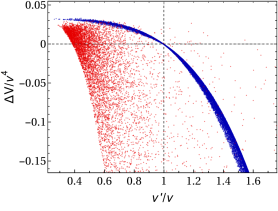
Figure 1: Left: Potential difference (4) at the two coexisting minima against $m^{2}_{12}$, both normalized by $v=246\,\mathrm{GeV}$. Right: The same depth difference against the ratio of non-standard vev (NV^′) to the standard vev (NV).

We confirm the approximation (10): for $\overline{\mathrm{ZB}}_{\pm}$ the sign of $m^{2}_{12}$ discriminates between our vacuum being the global minimum ($m^{2}_{12}>0$) or just a local metastable vacuum ($m^{2}_{12}<0$). This behavior, however, does not apply for the points (red) that deviate from the inert-like vacua, $\overline{\mathrm{ZP}}_{1,2}$, where the nonstandard vacuum may lie deeper despite $m^{2}_{12}$ being positive. For the generic values of $t_{\beta}$ as used above the density of non-regular coexisting minima is very low so that only a handful of coexisting non-regular minima is obtained jointly with the regular points. To generate a sufficient number of non-regular points we further produced another sample (most of the red points) by restricting $20\leq t_{\beta}\leq 50$ and positive $m^{2}_{12}$.

To accurately distinguish among the different cases, Ref. panic.vacuum constructed a very useful discriminant $D$ that ensures that our vacuum is always the global minimum if $D$ is positive. Since that discriminant was derived assuming that $v_{1},v_{2}$ are both positive, we cannot apply it to NV^′ when $v_{2}^{\prime}<0$. So we rederived the discriminant allowing the vevs to be negative with the result

$$D=\frac{1}{v^{4}}m^{2}_{12}(m^{2}_{11}-k^{2}m^{2}_{22})s_{2\beta}(t^{2}_{\beta}-k^{2})\,,$$ (17)

where $k\equiv(\lambda_{1}/\lambda_{2})^{1/4}$ and we have normalized to obtain a dimensionless quantity. This discriminant is useful because it can be obtained by using only the angle $\beta$ calculated in one vacuum and cases with only one minimum are automatically taken into account. The discriminating power of $D$ is shown in Fig. 2 where the depth difference is plotted against $D$ calculated using NV. Obviously we could have calculated the discriminant for NV^′, obtaining a $D^{\prime}$ with sign opposite to $D$. That implies that the quantity that depends on the vevs, $s_{2\beta}(t^{2}_{\beta}-k^{2})$, must have opposite signs when calculated for NV and NV^′.

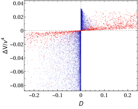
Figure 2: Normalized potential difference (4) at the two coexisting minima against the discriminant (17).

Our main goal here is to analyze if the discriminant power of $m^{2}_{12}$ and $D$ carries over to the one-loop effective potential.

III Effective potential at one-loop

We can now consider the effective potential

$$V=V_{0}+V_{1l}\,,$$ (18)

with the one-loop contribution

$$V_{1l}=\frac{1}{64\pi^{2}}\sum_{k}c_{k}M^{4}_{k}(\varphi_{i})\Big{(}\ln\frac{M_{k}^{2}(\varphi_{i})}{\mu^{2}}-\frac{3}{2}\Big{)}\,.$$ (19)

The masses $M^{2}_{k}(\varphi_{i})$ correspond to the scalar-field-dependent eigenvalues of the tree-level mass matrices of all particles of the theory while $\mu$ is the renormalization scale. We are already assuming a renormalization scheme with minimal subtraction ($\overline{\mathrm{MS}}$) and, for the gauge sector, the Landau gauge and dimensional reduction (DRED), following the scheme of Ref. martin . The parameters contained in $V_{0}$ are thus the renormalized parameters. The integer coefficients $|c_{k}|$ count all the degrees of freedom for each particle $k$ including color, charge and spin, while the sign of $c_{k}$ is determined by its boson/fermion character: positive for bosons and negative for fermions. For example, for the top quark we have $c_{t}=-3\times 2\times 2$ corresponding to its 3 colors, 2 particle/antiparticle and 2 spin degrees of freedom. We should note that the effective potential is generically a gauge dependent quantity but its value at an extremum is not nielsen .

As we will focus on normal vacua, we can consider that the effective potential depends only on the two real values $\varphi_{1},\varphi_{2}$ in the real neutral directions :

$$\phi_{1}=\frac{1}{\sqrt{2}}\begin{pmatrix}0\cr\varphi_{1}\end{pmatrix}\,,\quad\phi_{2}=\frac{1}{\sqrt{2}}\begin{pmatrix}0\cr\varphi_{2}\end{pmatrix}\,.$$ (20)

We reserve the symbols $v_{1},v_{2}$ in Eq. (2) to values at a minimum. So the field-dependent gauge boson masses retain the same functional form as in the SM with $v^{2}=v_{1}^{2}+v_{2}^{2}$:

$$M_{W}^{2}(\varphi_{i})=\mbox{\large$\tfrac{1}{4}$}g^{2}(\varphi_{1}^{2}+\varphi_{2}^{2})\,,\quad M_{Z}^{2}(\varphi_{i})=\mbox{\large$\tfrac{1}{4}$}(g^{2}+g^{\prime 2})(\varphi_{1}^{2}+\varphi_{2}^{2})\,.$$ (21)

The fermion masses depend on the type of 2HDM we are considering. We only consider models where FCNC are suppressed due to a $\mathbb{Z}_{2}$ symmetry. We focus more on the type I model but our results are equally valid for all types II, X and Y because of the dominance of the top Yukawa. For the type I we have

$$M_{t}(\varphi_{i})=\frac{y_{t}}{\langle s_{\beta}\rangle}\frac{\varphi_{2}}{\sqrt{2}}\,,\quad M_{b}(\varphi_{i})=\frac{y_{b}}{\langle s_{\beta}\rangle}\frac{\varphi_{2}}{\sqrt{2}}\,,$$ (22)

where $y_{t,b}$ are the Yukawa couplings of the third family quarks normalized to the SM values and the enhancement factor $1/\langle s_{\beta}\rangle$ should be considered as the fixed value at the NV minimum at one-loop. We emphasize that information with the bracket $\langle~{}~{}\rangle$. For the type II, we should replace the $M_{b}$ dependence on $\varphi_{2}$ and $\langle s_{\beta}\rangle$ by $\varphi_{1}$ and $\langle c_{\beta}\rangle$ respectively. We will see that, as usual, the top correction dominates the fermion loops and the difference between type I or type II is negligible for the one-loop corrections except for excessively large $\tan\beta$ which we do not consider. It is also justified that we only consider the effects of the top and bottom quarks; see Fig. 3 and comments in the text.

For the scalar contribution we need to calculate the eigenvalues of the matrix of second derivatives of $V_{0}$ for generic values of $\varphi_{i}$. These mass matrices are shown in appendix C and their eigenvalues correspond to $M^{2}_{S}(\varphi_{i})$ of the 8 scalars $S\in\{G^{\pm},H^{\pm},G^{0},A^{0},H^{0},h^{0}\}$. Due to charge and CP conservation, the mass matrices are still separated into three sectors: two charged scalars and its antiparticles, two CP odd scalars and two CP even scalars. We emphasize that e.g. $M^{2}_{G^{0}}(\varphi_{i})$ is nonvanishing at $\varphi_{i}$ away from any tree-level minimum. It is the second derivative of the whole effective potential at one-loop that will vanish in the directions of the Goldstone modes.

IV Parametrization and minimization at one-loop

We are interested in surveying the cases where the effective potential at one-loop (18) continues to have two local minima, one of which should be our vacuum with $v=\sqrt{v^{2}_{1}+v^{2}_{2}}=246\,\mathrm{GeV}$. The vevs $v_{1},v_{2}$ no longer satisfy the tree-level minimization relations in (5) but should now minimize the whole effective potential $V_{0}+V_{1l}$. We need a convenient parametrization to ensure that one minimum has the appropriate value of $v$.

To parametrize $V_{0}$, we will use as input the usual 8 quantities

$$\{v_{1},v_{2},\alpha,m^{2}_{H^{+}},m^{2}_{A},m^{2}_{H^{0}},m^{2}_{h},m^{2}_{12}\},$$ (23)

where $v_{i}$ satisfy the minimization equations (5). It is clear that these quantities define $V_{0}$ unambiguously by fixing the 8 parameters $\{m^{2}_{11},m^{2}_{22},m^{2}_{12},\lambda_{1},\lambda_{2},\lambda_{3},\lambda_{4},\lambda_{5}\}$; see e.g. the first reference in panic.vacuum . When we add the one-loop contribution, it is clear that the true minimum will be shifted by a small amount from the position $(v_{1},v_{2})$ at tree-level. Instead of correcting for that shift, we add the finite counterterms

$$\delta V=\delta m^{2}_{11}|\phi_{1}|^{2}+\delta m^{2}_{22}|\phi_{2}|^{2}\,,$$ (24)

to the potential and adjust the values of $\delta m^{2}_{ii}$ so that $v_{1},v_{2}$ continue to be a minimum at one-loop.  This means that the one-loop effective potential (18) is now rewritten as

$$V=V_{0}+\delta V+V_{1l}\,.$$ (25)

We can see that $\delta m^{2}_{ii}\to 0$ and $V_{1l}\to 0$ in the limit where we turn off all couplings of the scalars to other particles including self-couplings. For small couplings, it is also expected that the physical masses are close to the masses $\{m^{2}_{H^{+}},m^{2}_{A},m^{2}_{H^{0}},m^{2}_{h}\}$ used as input. It is possible to use a different renormalization scheme where all the masses and mixing angles at tree level are maintained at one-loop krause . Our scheme, however, avoids the need to deal with infrared divergences coming from the vanishing Goldstone masses cline ; 2hdm:PT:recent . This problem is more severe at higher loop orders martin.14 .

Now the minimization equations at one-loop can be separated into a tree-level part

$$\frac{1}{\varphi_{i}}\frac{\partial V_{0}}{\partial\varphi_{i}}\bigg{|}_{\varphi_{i}=v_{i}}=0\,,~{}~{}i=1,2,$$ (26)

which leads to the tree-level equations written in (5), and a one-loop part that defines $\delta m^{2}_{ii}$ by

$$-\delta m^{2}_{ii}=\frac{1}{\varphi_{i}}\frac{\partial V_{1l}}{\partial\varphi_{i}}\bigg{|}_{\varphi_{i}=v_{i}}\,,~{}~{}i=1,2.$$ (27)

We can separate the derivative of $V_{1l}$ into its contribution from scalars (S), vector bosons (V) and fermions (F):

$$\frac{1}{\varphi_{i}}\frac{\partial V^{S}_{1l}}{\partial\varphi_{i}}\bigg{|}_{\varphi_{i}=v_{i}} =\frac{1}{32\pi^{2}}\times\sum_{\begin{split}\mbox{\scriptsize$S=$}&\,\mbox{\scriptsize$G^{\pm},H^{\pm},G^{0},$}\\[-6.02777pt] &\,\mbox{\scriptsize$A^{0},H^{0},h^{0}$}\end{split}}\lambda_{iS}\,M^{2}_{S}\bigg{(}\ln\frac{M^{2}_{S}}{\mu^{2}}-1\bigg{)}\,,$$ (28)

$$\frac{1}{\varphi_{i}}\frac{\partial V^{V}_{1l}}{\partial\varphi_{i}}\bigg{|}_{\varphi_{i}=v_{i}} =\frac{3}{32\pi^{2}}\bigg{\{}\frac{g^{2}+g^{\prime 2}}{2}m^{2}_{Z}\bigg{[}\ln\frac{m^{2}_{Z}}{\mu^{2}}-1\bigg{]}+g^{2}m^{2}_{W}\bigg{[}\ln\frac{m^{2}_{W}}{\mu^{2}}-1\bigg{]}\bigg{\}}\,,$$

$$\frac{1}{\varphi_{i}}\frac{\partial V^{F}_{1l}}{\partial\varphi_{i}}\bigg{|}_{\varphi_{i}=v_{i}} =\frac{-4}{32\pi^{2}}\bigg{\{}\frac{3y_{t}^{2}}{\langle s_{\beta}\rangle^{2}}m^{2}_{t}\bigg{[}\ln\frac{m^{2}_{t}}{\mu^{2}}-1\bigg{]}+\frac{3y_{b}^{2}}{\langle s_{\beta}\rangle^{2}}m^{2}_{b}\bigg{[}\ln\frac{m^{2}_{b}}{\mu^{2}}-1\bigg{]}\bigg{\}}\,,$$

for each $i=1,2$. The dimensionless coefficients $\lambda_{iS}$ are given in appendix D and we use lowercase letters for $m_{W,Z,t,b}$ because they correspond to the actual values in the SM when we use our vacuum NV. For charged particles the contribution of the antiparticle can be taken into account by doubling the contribution of the particle. The fermion part corresponds to the type I model. For the type II model, we must replace $\langle s_{\beta}\rangle\to\langle c_{\beta}\rangle$ in the couplings to the $b$ quark. We can see in Fig. 3 that the contributions from scalars are large for $\delta m^{2}_{11}$ and $\delta m^{2}_{22}$ while the top contribution is also large and negative for $\delta m^{2}_{22}$. The contribution from the bottom quark is negligible for $\tan\beta\leq 50$ and there is no appreciable difference between the type I or type II model. Thus for definiteness we consider the type I model. We also note that the scalar masses and coefficients depend on $\delta m^{2}_{11},\delta m^{2}_{22}$ and (27) must be solved self-consistently.

The only remaining task is to write $M^{2}_{S}(v_{i})$ in terms of the input parameters (23). We note that $M^{2}_{S}(v_{i})$ should be computed from the second derivatives of $V_{0}+\delta V$. But the part coming from $V_{0}$ at $\varphi_{i}=v_{i}$ corresponds to the usual masses at tree-level because $(v_{1},v_{2})$ still corresponds to a minimum of $V_{0}$. Therefore, these matrices will have the generic form

$$\mathcal{M}(v_{i})=\mathcal{M}^{\rm tree}+\delta\mathcal{M}\,.$$ (29)

Specifically, the mass matrices for the different sectors read

$$\mathcal{M}_{\rm char}(v_{i})=m^{2}_{H^{+}}\begin{pmatrix}s^{2}_{\beta}&-s_{\beta}c_{\beta}\cr-s_{\beta}c_{\beta}&c^{2}_{\beta}\end{pmatrix}+\begin{pmatrix}\delta m^{2}_{11}&\cr&\delta m^{2}_{22}\end{pmatrix}\,,$$ (30)

$$\mathcal{M}_{\rm odd}(v_{i})=m^{2}_{A}\begin{pmatrix}s^{2}_{\beta}&-s_{\beta}c_{\beta}\cr-s_{\beta}c_{\beta}&c^{2}_{\beta}\end{pmatrix}+\begin{pmatrix}\delta m^{2}_{11}&\cr&\delta m^{2}_{22}\end{pmatrix}\,,$$ (31)

$$\mathcal{M}_{\rm even}(v_{i})=\left(\begin{array}[]{cc}\lambda_{1}v^{2}c_{\beta}^{2}+m^{2}_{12}t_{\beta}&-m^{2}_{12}+\lambda_{345}v^{2}s_{\beta}c_{\beta}\\ -m^{2}_{12}+\lambda_{345}v^{2}s_{\beta}c_{\beta}&\lambda_{2}v^{2}s^{2}_{\beta}+m^{2}_{12}\,\cot_{\beta}\\ \end{array}\right)+\begin{pmatrix}\delta m^{2}_{11}&\cr&\delta m^{2}_{22}\end{pmatrix}\,,$$ (32)

where $m^{2}_{H^{+}}=\frac{m^{2}_{12}}{c_{\beta}s_{\beta}}-\mbox{\large$\tfrac{1}{2}$}v^{2}\lambda_{45}$ and $m^{2}_{A}=\frac{m^{2}_{12}}{c_{\beta}s_{\beta}}-v^{2}\lambda_{5}$ are the masses squared for the charged Higgs and the pseudoscalar at tree-level; see e.g. branco.rev . Clearly the first and second matrices contain each a vanishing eigenvalue corresponding to the charged ($G^{\pm}$) and neutral ($G^{0}$) Goldstone bosons in the limit where $\delta m^{2}_{ii}\to 0$. We use the basis $(\phi_{1}^{+},\phi_{2}^{+})$, $(\sqrt{2}\operatorname{\mathrm{Im}}\phi_{1}^{0},\sqrt{2}\operatorname{\mathrm{Im}}\phi_{2}^{0})$ and $(\sqrt{2}\operatorname{\mathrm{Re}}\phi_{1}^{0},\sqrt{2}\operatorname{\mathrm{Re}}\phi_{2}^{0})$ in Eqs. (30), (31) and (32), respectively, from the parametrization $\phi_{i}=(\phi_{i}^{+},\phi_{i}^{0})^{\mbox{\scriptsize$\mathsf{T}$}}$.

Diagonalization of the tree-level part of $\mathcal{M}_{\rm even}(v_{i})$ defines the angle $\alpha$ through

$$U_{\alpha}^{\dagger}\mathcal{M}_{\rm even}^{\rm tree}U_{\alpha}=\operatorname{\mathrm{diag}}(m^{2}_{H^{0}},m^{2}_{h^{0}})\,,$$ (33)

where

$$U_{\alpha}=\begin{pmatrix}c_{\alpha}&-s_{\alpha}\cr s_{\alpha}&c_{\alpha}\end{pmatrix}\,.$$ (34)

Using the same notation we can find the eigenvalues shifted by $\delta m^{2}_{ii}$ as

$$U_{\beta_{+}}^{\dagger}\mathcal{M}_{\rm char}(v_{i})U_{\beta_{+}} =\operatorname{\mathrm{diag}}(M^{2}_{G^{+}},M^{2}_{H^{+}})\,,$$ (35)

$$U_{\beta_{0}}^{\dagger}\mathcal{M}_{\rm odd}(v_{i})U_{\beta_{0}} =\operatorname{\mathrm{diag}}(M^{2}_{G^{0}},M^{2}_{A^{0}})\,,$$

$$U_{\alpha^{\prime}}^{\dagger}\mathcal{M}_{\rm even}(v_{i})U_{\alpha^{\prime}} =\operatorname{\mathrm{diag}}(M^{2}_{H^{0}},M^{2}_{h^{0}})\,,$$

where the angles $\beta_{+},\beta_{0},\alpha^{\prime}$ are shifted from $\beta,\beta,\alpha$ by a small amount due to $\delta m^{2}_{ii}$:

$$\beta_{+}=\beta+\delta\beta_{+},\quad\beta_{0}=\beta+\delta\beta_{0},\quad\alpha^{\prime}=\alpha+\delta\alpha.$$ (36)

The explicit forms for $\delta\beta_{+,0}$ and $\delta\alpha$ can be seen in appendix D.

V Pole masses at one-loop

The previous section showed a way of ensuring that one of the minima of the effective potential at one-loop corresponded to our vacuum with $v=246\,\mathrm{GeV}$ and that $\tan\beta=v_{2}/v_{1}$ could be used as input at one-loop. The following task to describe a realistic 2HDM at one-loop is to ensure that the SM higgs boson mass corresponds to the experimentally measured value pdg :

$$m_{h}\big{|}_{\rm exp}=125.09\pm 0.24\,\mathrm{GeV}\,.$$ (37)

It is clear that at one-loop we cannot use this value for the tree-level parameter $m_{h}$ in (23). Instead, we must check that the pole mass corresponds to (37).

We follow Ref. (martin, , b) to calculate the pole masses $\hat{m}_{S}$ of all the scalars $S$ including the SM higgs boson by computing the self-energies of the theory at one-loop. We focus in this section on the CP even sector which will give rise to the pole masses of $h$ and $H$ restricted to the case $\hat{m}_{H}>\hat{m}_{h}$. The self-energy for the other sectors are given in appendix F.

The scalar self-couplings can be extracted from $V_{0}$. Given a set of real scalars $S_{i}$ that interact through the quartic vertex $-ig_{ijkl}$ and cubic vertex $-ig_{ijk}$, the self-energy $\Pi_{ij}$ for $S_{i}$–$S_{j}$ coming from scalars in the loop with incoming momentum $p^{2}=s$ is given by martin

$$16\pi^{2}\Pi_{ij}^{S}(s)=\mbox{\large$\tfrac{1}{2}$}\sum_{k}g_{ijkk}A(m_{k})+\mbox{\large$\tfrac{1}{2}$}\sum_{kl}g^{2}_{ijkl}B(m_{k},m_{l},s)\,,$$ (38)

assuming we are in the basis with diagonalized masses (quadratic part of $V_{0}+\delta V$). The $A$ and $B$ functions are the Passarino-Veltman functions PV which, in the notation of Ref. pedro , read

$$A(m) \equiv m^{2}\left[\log\left(\frac{m^{2}}{\mu^{2}}\right)\,-\,1\right],$$ (39)

$$B(m_{1},m_{2},s) \equiv \int^{1}_{0}\,dt\,\log\left[\frac{t\,m_{1}^{2}\,+\,(1-t)\,m_{2}^{2}\,-\,t(1-t)s}{\mu^{2}}\right].$$ (40)

The $A$ function represents the one-loop graph with one quartic vertex (tadpole) and the $B$ function represents the one-loop graph with two vertices and two internal lines. Hence the factors $1/2$ are the symmetry factors that appear in front of the Feynman diagrams for identical fields. These functions appear after renormalizing these diagrams using the $\overline{\mathrm{MS}}$ prescription. Simplifications for vanishing $s$ can be found in Ref. pedro . The contributions coming from gauge bosons and fermions in the loop are also shown in appendix F and all the necessary cubic and quartic couplings of the theory are explicitly shown in appendix E.

For example, the SM higgs self-energy is given by

$$16\pi^{2}\Pi^{S}_{hh}(s) =\mbox{\large$\tfrac{1}{2}$}\sum_{S=G^{0},A,H,h}g_{h^{2}S^{2}}A(M_{S})+\sum_{S=G^{+},H^{+}}g_{h^{2}S\bar{S}}A(M_{S})$$ (41)

$$\quad+\mbox{\large$\tfrac{1}{2}$}\sum_{S,S^{\prime}=G^{0},A,H,h}g_{hSS^{\prime}}^{2}B(M_{S},M_{S^{\prime}},s)+\sum_{S,S^{\prime}=G^{+},H^{+}}|g_{hS\bar{S^{\prime}}}|^{2}B(M_{S},M_{S^{\prime}},s)\,,$$

where $g_{h^{2}h^{2}}=g_{h^{4}}$ and $g_{hh^{2}}=g_{h^{3}}$ are the quartic and cubic self-couplings for $h$ and all $M_{S}$ refer to $M_{S}(v_{i})$. However, the mixing to the other CP even scalar $H$ in $\Pi_{Hh}$ cannot be neglected.

Due to charge and CP conservation, the self-energy for the different scalars decouple into separate pieces for the CP even, CP odd and charged sectors. The self-energy for the CP even sector is given by the matrix

$$\Pi^{\rm even}(s)=\begin{pmatrix}\Pi_{HH}(s)&\Pi_{Hh}(s)\cr\Pi_{hH}(s)&\Pi_{hh}(s)\end{pmatrix}\,.$$ (42)

The one-loop pole squared masses $\hat{m}_{H}^{2},\hat{m}_{h}^{2}$ for the CP even scalars $H,h$ are the solutions $s_{k}$ for martin

$$\det\begin{pmatrix}M_{H}^{2}+\operatorname{\mathrm{Re}}\Pi_{HH}(s_{k})-s_{k}&\operatorname{\mathrm{Re}}\Pi_{Hh}(s_{k})\cr\operatorname{\mathrm{Re}}\Pi_{hH}(s_{k})&M_{h}^{2}+\operatorname{\mathrm{Re}}\Pi_{hh}(s_{k})-s_{k}\end{pmatrix}=0\,,$$ (43)

where we take only the real part of the self-energy because we are not interested in the decay widths. The $\hat{m}_{h}^{2}$ corresponds to the solution that continually approaches $M_{h}^{2}$ in the limit where we turn off the interactions. A similar consideration applies to all pole squared masses.

VI Numerical survey

We describe here the procedure we used to survey the models. For definiteness, we adopted the relevant fixed parameters of the SM to be

$$g=0.6483;\quad g^{\prime}=0.3587;\quad v=246.954\;\mathrm{GeV};\quad y_{t}=0.93697;\quad y_{b}=0.023937\,.$$ (44)

The first four values were taken from Refs. strumia ; martin.14 as the running parameters of the SM at the top pole mass $\mu=173.34\,\mathrm{GeV}$ and the bottom Yukawa was adapted from its mass value $m_{b}=4.18\,\mathrm{GeV}$ pdg . Among these parameters, only the top Yukawa appreciably affects the one-loop effective potential together with the quartic scalar self-couplings. We use a fixed renormalization scale $\mu=300\,\mathrm{GeV}$ for all calculations and note that the running of $y_{t}$ from the top mass scale only amounts to a small difference. The running for the rest of the parameters are even less relevant. We remark that any choice of the renormalization scale is allowed, since the difference in depth of the potential at two extrema is a renormalization scale-independent quantity scale . However, from a practical point of view, it is desirable that the logarithms in the effective potential do not become too “large” so as to lead to numerical instabilities casas . We have checked our calculation for some different values of the renormalization scale and the value of $\mu=300\,\mathrm{GeV}$ proved to be a stable choice.

Among the input parameters in (23), we fixed the standard vev $v$ as above and took the rest of the parameters randomly in the range shown in the first row of Table 1, restricted to $m_{H}>m_{h}$. After checking for simple perturbativity and bounded from below conditions at tree-level, we picked only the points where the shifted masses squared $M_{S}^{2}(v_{i})$ were positive and the solutions for the shift $\delta m^{2}_{ii}$ in (27) were real. Then we further selected only the points where the pole mass $\hat{m}_{h}$ calculated as in Sec. V fell in the experimental range of (37). In this way, we generated the sample G with 294437 points among which 4525 had two minima at one-loop, 17 of which were non-regular. To find the second minimum, we explicitly minimized the real part of the effective potential (18) starting from the non-standard minimum at tree-level and then retained only the points where the value of the potential at that minimum was real weinberg.wu . Given the small number of non-regular points, we generated another sample denoted as NR focusing only on non-regular points by imposing large $t_{\beta}$ as in the second row of Table 1; other ranges were kept the same, except for $m^{2}_{12}$ which was chosen positive. Sample NR thus contained 185905 points among which 1563 had two minima at one-loop. Hereafter, unless explicitly specified, we will consider only the joint sample of G and NR. However, we would like to emphasize that, even though samples G and NR have a similar number of points, the parameter space scanned by sample NR represents only a small portion of the parameter space probed by sample G. This justifies our definition of non-regular points.

$$\begin{array}[]{|c|c|c|c|c|c|c|c|}\hline\cr\text{Sample}&t_{\beta}&\cos(\beta-\alpha)&m_{H^{+}}\,(\mathrm{GeV})&m_{A}\,(\mathrm{GeV})&m_{H}\,(\mathrm{GeV})&m_{h}\,(\mathrm{GeV})&m^{2}_{12}\,(\mathrm{GeV^{2}})\cr\hline\cr\text{G}&\phantom{2}1\div 50&-0.1\div 0.1&90\div 1000&90\div 1000&90\div 1000&0\div 150&-6000\div 6000\cr\hline\cr\text{NR}&20\div 50&\text{--}&\text{--}&\text{--}&\text{--}&\text{--}&\phantom{-600}0\div 6000\cr\hline\cr\end{array}$$

Table 1: Input parameter ranges for the general sample (G) and non-regular points (NR). The dash denotes the same range as in the previous row.

After the selections described above, the input parameters $m_{H^{+}},m_{A},m_{H}$ get roughly confined to the range $[90,500]$ and the non-standard higgsses acquire pole masses in a similar range with slightly smaller maximal value for $\hat{m}_{H^{+}}$. In contrast, the distribution for $t_{\beta}$ is homogeneous in the range of Table 1 for the whole sample but, as we select only the points with two minima at one-loop, it gets separated into two ranges, $1\leq t_{\beta}\lesssim 3.8$ for the regular minima, and $24\lesssim t_{\beta}\leq 50$ for the non-regular ones.

To check our numerically implemented formulas, we performed the following consistency checks:

1. Vanishing of the pole masses for the Goldstone bosons $G^{\pm},G^{0}$ for zero external momentum for the three cases where we successively add the one-loop scalar, vector boson and fermion contributions.

2. Equality of the pole masses for the CP even higgsses $H,h$ for zero external momentum and the eigenvalues of the explicitly calculated second derivative matrix of the effective potential in the real neutral directions (20) in all three cases of successive addition of the one-loop scalar, vector boson and fermion contributions.

VII Results

Let us first quantify the shifts $\delta m^{2}_{ii}$ in (27) for the different contributions. The contribution coming from the gauge bosons only depends on the value of $v$ and, for fermions, it depends on $v$ and $\beta$. The scalar contribution depends on many parameters coming from the scalar potential. The dependence of the different contributions on $\tan\beta$ are shown in Fig. 3. We can see that the dominant contribution for $\delta m^{2}_{11}$ comes from the scalars whereas $\delta m^{2}_{22}$ also has large positive contributions from scalars but they are partly canceled by the negative contribution from fermions (top). Such a partial cancellation in $\delta m^{2}_{22}$ can be clearly seen in Fig. 4 where we show the contribution only from scalars (green points) and all the contributions (red points). The orange curve in Fig. 3, which quantifies the bottom contribution to $\delta m^{2}_{11}$ in the type II model, shows that it is negligible in the range of $\tan\beta$ we are interested in and our calculation that uses the type I model applies equally well to the type II case. All the different contributions are calculated using Eq. (28) and the scalar contribution in particular depends on the $\delta m^{2}_{ii}$ themselves and these are taken as the total contributions. The remaining contributions of gauge bosons (purple dashed curve in Fig. 3) are much smaller. The contribution from scalars are calculated using the whole sample (G $+$ NR) described in Sec. VI which also includes the points with only one vacuum.

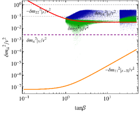
Figure 3: Different contributions for $\delta m^{2}_{ii}$ in (27). The scalar contributions are positive for $\delta m^{2}_{11}$ (blue points) and mostly positive for $\delta m^{2}_{22}$ (green points) while the fermions contribute negatively. The fermion contribution to $\delta m^{2}_{22}$ (red curve) is practically the same for the type I and II models while the contribution to $\delta m^{2}_{11}$ (orange curve) applies only to the type II case but vanishes for the type I case. The contributions from the gauge bosons are shown in the purple dashed line.

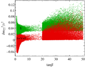
Figure 4: Different contributions to $\delta m^{2}_{22}$ in (27): the green points quantify the scalar contribution only whereas the red points consider all the contribution in the type I or II model.

The deviation of the location of our vacuum when we add $\delta V$ do $V_{0}$ is illustrated in Fig. 5 where we show the ratio of $t_{\beta}$ for $V_{0}+\delta V$ ($t_{\beta}^{\rm tree+\delta}$) to that of $V_{0}$ ($t_{\beta}$) against the ratio of the vev for $V_{0}+\delta V$ ($v_{\rm tree+\delta}$) to that of $V_{0}$ ($v$). We only show the points with two coexisting minima and divide the points between the regular ones (blue) and the non-regular ones (red). We can see that as $m_{ii}^{2}$ get shifted by $\delta m^{2}_{ii}$ all points with two minima have their vevs decreased while $t_{\beta}$ mostly increases for the regular points and mostly decreases for the non-regular points. Note that the non-regular points only consider large $t_{\beta}$ whereas the regular points only include moderate $t_{\beta}$ roughly up to $3.8$. As the location of $(v_{1},v_{2})$ for our vacuum is the same for $V_{0}$ and the one-loop corrected potential (25) we can also interpret this plot as the modification of the vev location of $V_{0}+\delta V$ compared to $V_{0}+\delta V+V_{1l}$. If we had considered all the points including the points with only our vacuum, the majority of points would follow the behavior of the regular points in blue.

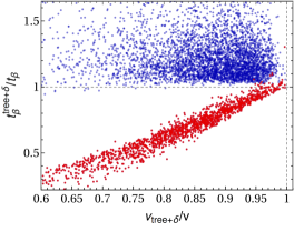
Figure 5: Variation of $t_{\beta}$ and $v$ when shifting the quadratic parameters $m_{ii}^{2}$ of (1) by $\delta m^{2}_{ii}$. The blue (red) points represent (non-)regular points.

For the case of coexisting vacua, we can see a clear difference in behavior between the regular points and the non-regular ones in Fig. 6 where we plot the potential difference with respect to $m^{2}_{12}$. The left panel shows these quantities using the tree-level potential $V_{0}$ while the right panel is the same plot for the one-loop potential (25). We can clearly see that the potential difference goes continuously to zero as $m^{2}_{12}\to 0$ for the blue points representing the regular minima. Moreover, for positive $m^{2}_{12}$ our vacuum is guaranteed to be the global minimum in both tree level or one-loop potential. This behavior is opposite for negative $m^{2}_{12}$. The reason is that only $m^{2}_{12}$ breaks explicitly the $\mathbb{Z}_{2}$ symmetry of the theory and it controls the degeneracy breaking of the spontaneously breaking minima. This behavior is not followed by the non-regular minima that do not have degenerate minima in the $m^{2}_{12}\to 0$ limit. Some points (green) in which our vacuum is not the global one at tree-level even get inverted and become the global minimum as the one-loop corrections are added. The same conclusion is reached if we had compared the one-loop potential to $V_{0}+\delta V$ instead: some cases where our minimum is not the deepest at tree-level becomes the global minimum at one-loop.

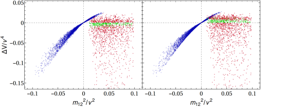
Figure 6: Potential difference of the two coexisting minima against $m_{12}^{2}$. Left: Only the tree level potential (1) is considered. This plot should be compared with Fig. 1. Right: The full 1-loop effective potential (25) is considered. The green points represent a change in sign of the tree level prediction for the potential difference.

We can have an idea of the different one-loop contributions in Fig. 7 where we separate the potential difference in Fig. 6 into its different contributions. Regarding the regular points (left plot), it can be seen that the one-loop potential difference is almost entirely due to the tree-level contribution (blue) since the contributions from $\delta V$ (yellow), fermions (red) and scalars (purple) approximately cancel each other while the contribution from gauge bosons (green) is negligible compared to the others. This behavior justifies our choice for the renormalization scale. For the non-regular points (right plot), no clear pattern emerges. We can also see in Fig. 8 that there are points where the potential difference is raised as well as points where it is lowered by the one-loop corrections for both regular and non-regular points.

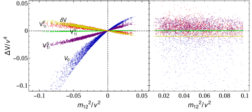
Figure 7: Different contributions coming from the tree level potential (blue), $\delta V$ (yellow), fermions (red), scalars (purple), and vectors bosons (green) to the one-loop potential difference of the right panel of Fig. 6. In the left plot only regular points are considered while the right plot shows the behavior of the non-regular ones.

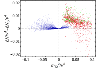
Figure 8: One-loop correction to the potential difference relative to the tree level potential difference. The color coding follows Fig. 6.

Considering that the discriminant (17) test is applicable for all cases where at least one normal vacuum is known, we can investigate if it is still a good predictor for the one-loop potential with two coexisting minima. We can adapt the tree-level discriminant to one-loop in the following three ways:

$$D_{1} =\text{Eq.\,}\eqref{discriminant}\,,$$ (45)

$$D_{2} =\text{Eq.\,}\eqref{discriminant}\big{|}_{m^{2}_{ii}\to m^{2}_{ii}+\delta m^{2}_{ii},\,v\to v^{(0)},\,\beta\to\beta^{(0)}}\,,$$

$$D_{3} =\text{Eq.\,}\eqref{discriminant}\big{|}_{m^{2}_{ii}\to m^{2}_{ii}+\delta m^{2}_{ii}}\,.$$

The quantity $D_{1}$ is the discriminant calculated with $V_{0}$ as the whole potential while $D_{2}$ is calculated by using $V_{0}+\delta V$ in (25). In the latter case, the quadratic parameters $m^{2}_{ii}$ get shifted and the location of the minimum, denoted above as $(v^{(0)},\beta^{(0)})$ or as $\rm tree+\delta$ (superscript/subscript) in Fig. 5, do not coincide with the ones used as input, denoted as $(v,\beta)$. The last adaptation $D_{3}$ considers the shifts in the quadratic parameters but keeps the vevs as $(v,\beta)$. We will test here if any of these discriminants are capable of distinguishing if our vacuum is the global one at one-loop only using parameters at tree-level.

For the regular coexisting minima, Fig. 6 shows that $m^{2}_{12}$ is already a good predictor of the global minimum, but we can test the discriminants in (45). The result of this test is shown in Fig. 9 where the potential difference at one-loop is plotted against the three discriminants. We can see in the left and middle plots that $D_{1}$ and $D_{2}$ correctly predict the global minimum of the one-loop effective potential while the right plot shows that $D_{3}$ fails for more than 10$\%$ of the points.

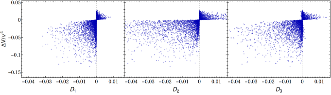
Figure 9: Comparison of the three discriminants proposed in (45) in the case of regular points.

In constrast, the failure of all the discriminants (45) for the non-regular points (of samples G and NR) can be seen in Fig. 10 which shows the potential depth difference as a function of the discriminants, similarly to the regular points in Fig. 9; note that the horizontal scale is very different. The green points in the second and fourth quadrants mark the cases where the discriminant $D_{1}$ predicts the opposite behavior at one-loop. We can clearly see that all discriminants fail for a significant portion of points, not necessarily for the same ones. From the property of $D_{1}$, we could have seen its wrong prediction in Fig. 6 as well.

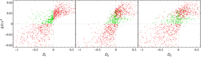
Figure 10: Comparison of the three discriminants proposed in (45) in the case of non-regular points. The green points mark the cases where $D_{1}$ predicts the opposite depth difference.

At last, to make sure that the points for which the discriminant test fails include phenomenologically realistic points, we have checked the viability of the red/green points in Fig. 6 by considering phenomenological constraints implemented in the 2HDMC code 2HDMC . We found that in the case of the type I model around half of the green points are allowed by experimental constraints such as the S, T, U precision electroweak parameters and data from colliders implemented in the HiggsBounds and HiggsSignals packages HB ; HS , while in the type II model they are all excluded. For the type II model we have also included constraints coming from $R_{b}$ measurements constrain_R:H+ as well as $B$ meson decays constrain:H+ which prove to be very strong by setting $m_{H^{+}}>480\,\mathrm{GeV}$ independently of the value of $\tan\beta$. For type I, since the red/green points have $\tan\beta>10$, these constraints do not impose any further restrictions constrain_g:H+ . We also checked that all points still respect simple bounded from below and perturbativity constraints branco.rev .

VIII Conclusions

We have studied the one-loop properties of the real Two-Higgs-doublet model with softly broken $\mathbb{Z}_{2}$ with respect to the possibility of two coexisting normal vacua. The softly broken nature must remain at one-loop and the case of two coexisting normal minima can be classified into two very distinct types depending on their nature in the vanishing $m^{2}_{12}$ limit: regular minima that spontaneously break the symmetry and the non-regular minima (or minimum) that preserve the symmetry, i.e., they are inert-like in the symmetric limit. Since in the first case the two minima are degenerate in the symmetry limit, even at one-loop, they are connected by the $\mathbb{Z}_{2}$ symmetry and then they should differ only by the sign of $v_{2}$. After the inclusion of the $m^{2}_{12}$ term, the sign of $v_{2}$ continue to be opposite for our vacuum and the non-standard one so that the two regular minima are found in the first and fourth quadrants in the $(v_{1},v_{2})$ plane. In contrast, the non-regular minima deviate from the inert-like minima and both deviate to the first quadrant when $m^{2}_{12}$ is positive.

The vacua that spontaneously break $\mathbb{Z}_{2}$ in the $m^{2}_{12}\to 0$ limit behave rather regularly and we can distinguish which coexisting minimum is the global one by just examining the sign of $m^{2}_{12}$: when it is negative our vacuum is only a metastable local one and the opposite is true if it is positive. For this type of coexisting vacua, the discriminant at tree level [$D_{1,2}$ in Eq. (45)] is still a good predictor of the nature of the minimum it is calculated with.

For the non-regular coexisting vacua, $m^{2}_{12}$ is positive in the convention that our vacuum has both vevs positive and it cannot be used as an indicator. At tree level, the discriminant of Ref. panic.vacuum is a very convenient way of testing if our vacuum is the global one because only the location of our minimum is required. However, at one-loop, this discriminant is not a precise indicator of which minima is the global one. We have found realistic cases where our vacuum is not the global minimum at tree-level but it becomes the global one after the addition of the one-loop corrections. Few cases for the opposite behavior were also found. As the discriminant effectively distinguishes the sign of the potential difference between the coexisting minima at tree-level, the latter itself is also a not good indicator for the non-regular minima. This is reminiscent of the exact $\mathbb{Z}_{2}$ symmetric case (inert model) investigated in Ref. pedro . On the other hand, we were unable to find a discriminant that works for both regular and non-regular minima at one-loop. Finding a simple and precise criterion for global minimum does not seem to be an easy task as that was not achieved even in the simpler exact $\mathbb{Z}_{2}$ limit. We also emphasize that for our parametrization which enforces our vacuum to be a minimum from the start, and for the chosen generic ranges of parameters (sample G), the occurrence of non-regular minima, as suggested by its name, is much rarer: only $38\%$ correspond to the non-regular cases and, among then, only $0.3\%$ are coexisting minima.

In summary, the soft-breaking term $m^{2}_{12}$ controls the lifting of the degeneracy of the regular coexisting minima (moderate $\tan\beta$) even at one-loop and can be used as the sole indicator of which minimum is the global one. That is not true when two coexisting non-regular vacua (large or small $\tan\beta$) exist: the discriminant that is a precise indicator at tree-level is not reliable at one-loop and explicit calculation of the potential depths must be carried out.

Appendix A Deviation of a potential minimum

Take a potential $V_{0}(\varphi)$ depending on real scalar fields $\varphi_{i}$ for which we know a minimum (extremum) $\varphi_{i}=\bar{\varphi}_{i}$ satisfying

$$\frac{\partial V_{0}(\bar{\varphi})}{\partial\varphi_{i}}=0\,.$$ (46)

We want to quantify how the location of the minimum and the value of the potential deviate when we add a small perturbation $U$ on the potential as

$$V=V_{0}+U\,.$$ (47)

We assume $V_{0}$ has no flat direction around $\bar{\varphi}$.

We first quantify the deviation of the location of the minimum as

$$\varphi_{i}=\bar{\varphi}_{i}+\delta\varphi_{i}\,.$$ (48)

The derivative of the perturbed potential gives

$$\frac{\partial V_{0}(\bar{\varphi}+\delta\varphi)}{\partial\varphi_{i}}=\frac{\partial V_{0}(\bar{\varphi})}{\partial\varphi_{i}}+\frac{\partial U(\bar{\varphi})}{\partial\varphi_{i}}+\frac{\partial^{2}V_{0}(\bar{\varphi})}{\partial\varphi_{i}\partial\varphi_{j}}\delta\varphi_{j}+O(\delta^{2})\,.$$ (49)

Since the first term vanishes due to (46), we get the deviation to first order

$$\delta\varphi_{j}=-\mathcal{M}^{-1}_{ji}U_{i}\,,$$ (50)

where $U_{i}\equiv\partial U(\bar{\varphi})/\partial\varphi_{i}$ and $\mathcal{M}_{ij}=\frac{\partial^{2}V_{0}(\bar{\varphi})}{\partial\varphi_{i}\partial\varphi_{j}}$ is the squared-mass matrix around $\bar{\varphi}$.

The deviation in the value of the minimum can be equally expanded around $\bar{\varphi}$ as

$$V(\bar{\varphi}+\delta\varphi)=V_{0}(\bar{\varphi})+U(\bar{\varphi})-\mbox{\large$\tfrac{1}{2}$}U_{i}\mathcal{M}^{-1}_{ij}U_{j}+O(\delta^{3})\,,$$ (51)

after using (50). Generically the third term contributes to deepen the potential. That is the dominant contribution when the perturbation vanishes on the unperturbed minimum: $U(\bar{\varphi})=0$. The latter happens for the $m^{2}_{12}$ term when perturbing the inert-like minima while for the spontaneously broken $\mathbb{Z}_{2}$ minima the dominant term is the second, linear in the perturbation.

Appendix B Finding more than one normal vacua

Let us rewrite the minimization equations in Eq. (5) as

$$A_{\zeta}X=M\,,$$ (52)

where

$$A_{\zeta}=\begin{pmatrix}\lambda_{1}&\lambda_{345}-\zeta\cr\lambda_{345}-\zeta&\lambda_{2}\end{pmatrix}\,,\quad X=\begin{pmatrix}v_{1}^{2}\cr v_{2}^{2}\end{pmatrix}\,,\quad M=-2\begin{pmatrix}m^{2}_{11}\cr m^{2}_{22}\end{pmatrix}\,,$$ (53)

and $\zeta\equiv 2m^{2}_{12}/v_{1}v_{2}$ depends on the vevs.

To find solutions $(v_{1},v_{2})$ of (52) for $m^{2}_{12}\neq 0$, we first need an equation for $\zeta$. For that end, we can formally write (52) as $X=A_{\zeta}^{-1}M$ and equate $v_{1}^{2}v_{2}^{2}=4m^{4}_{12}/\zeta^{2}$. We obtain

$$\frac{m^{4}_{12}}{\zeta^{2}}\big{[}(\lambda_{345}-\zeta)^{2}-\lambda_{1}\lambda_{2}\big{]}^{2}=[m^{2}_{11}\zeta-\mu_{1}][m^{2}_{22}\zeta-\mu_{2}]\,,$$ (54)

where $\mu_{1}=\lambda_{345}m^{2}_{11}-\lambda_{1}m^{2}_{22}$ and $\mu_{2}=\lambda_{345}m^{2}_{22}-\lambda_{2}m^{2}_{11}$. The $m^{2}_{12}\to 0$ limit is taken as $\zeta\to 0$ and $\frac{m^{4}_{12}}{\zeta^{2}}\to v_{1}^{2}v_{2}^{2}/4$. When $m^{2}_{12}\neq 0$, we can find the possible values for $\zeta$ (extrema) from the quartic equation

$$m^{4}_{12}\big{[}(\lambda_{345}-\zeta)^{2}-\lambda_{1}\lambda_{2}\big{]}^{2}=\zeta^{2}[m^{2}_{11}\zeta-\mu_{1}][m^{2}_{22}\zeta-\mu_{2}]\,.$$ (55)

We know there are at most four real solutions coinciding with the maximal number of extrema in this case ivanov:mink . We also can see that the root $\lambda_{345}+\sqrt{\lambda_{1}\lambda_{2}}$ from the lefthandside is always positive due to bounded below conditions. Possible solutions for (52) depends on the sign of $\zeta$ and we allow both signs for $v_{1}v_{2}$. We can see that for the same $\zeta$, flipping the sign of $m^{2}_{12}$ is equivalent to flipping the sign of $v_{1}v_{2}$.

Once some solution $\zeta=\zeta_{0}$ is found, we can find the vevs from the relation $X=A_{\zeta}^{-1}M$ or, explicitly,

$$v_{1}^{2} =\frac{2(m^{2}_{22}\zeta-\mu_{2})}{(\lambda_{345}-\zeta)^{2}-\lambda_{1}\lambda_{2}}~{}>0\,,$$ (56)

$$v_{2}^{2} =\frac{2(m^{2}_{11}\zeta-\mu_{1})}{(\lambda_{345}-\zeta)^{2}-\lambda_{1}\lambda_{2}}~{}>0\,.$$

After ensuring these expression are positive, we can extract $v_{1},v_{2}$ and $\tan\beta$ with the sign convention where $v_{1}>0$ and

$$\operatorname{sign}(v_{2})=\operatorname{sign}(\zeta m^{2}_{12})\,.$$ (57)

Appendix C Matrix of second derivatives

The mass matrices at tree-level for the charged, CP-odd and CP-even scalar sectors prior to imposing the minimization conditions are given respectively by

$$\mathcal{M}_{\rm char}(\varphi_{i})=\langle\frac{\partial^{2}V_{0}}{\partial\phi_{a}^{-}\partial\phi_{b}^{+}}\rangle=\left(\begin{array}[]{cc}\mbox{\large$\tfrac{1}{2}$}\lambda_{1}\varphi_{1}^{2}+\mbox{\large$\tfrac{1}{2}$}\lambda_{3}\varphi_{2}^{2}&\frac{1}{2}\lambda_{45}\varphi_{1}\varphi_{2}\\ \frac{1}{2}\lambda_{45}\varphi_{1}\varphi_{2}&\mbox{\large$\tfrac{1}{2}$}\lambda_{2}\varphi_{2}^{2}+\mbox{\large$\tfrac{1}{2}$}\lambda_{3}\varphi_{1}^{2}\\ \end{array}\right)+(\text{quadratic})\,,$$ (58)

$$\mathcal{M}_{\rm odd}(\varphi_{i})=\langle\frac{\partial^{2}V_{0}}{\partial\eta_{a}\partial\eta_{b}}\rangle=\left(\begin{array}[]{cc}\mbox{\large$\tfrac{1}{2}$}\lambda_{1}\varphi_{1}^{2}+\mbox{\large$\tfrac{1}{2}$}\bar{\lambda}_{345}\varphi_{2}^{2}&\lambda_{5}\varphi_{1}\varphi_{2}\\ \lambda_{5}\varphi_{1}\varphi_{2}&\mbox{\large$\tfrac{1}{2}$}\lambda_{2}\varphi_{2}^{2}+\mbox{\large$\tfrac{1}{2}$}\bar{\lambda}_{345}\varphi_{1}^{2}\\ \end{array}\right)+(\text{quadratic})\,,$$ (59)

$$\mathcal{M}_{\rm even}(\varphi_{i})=\langle\frac{\partial^{2}V_{0}}{\partial\rho_{a}\partial\rho_{b}}\rangle=\left(\begin{array}[]{cc}\mbox{\large$\tfrac{3}{2}$}\lambda_{1}\varphi_{1}^{2}+\mbox{\large$\tfrac{1}{2}$}\lambda_{345}\varphi_{2}^{2}&\lambda_{345}\varphi_{1}\varphi_{2}\\ \lambda_{345}\varphi_{1}\varphi_{2}&\mbox{\large$\tfrac{3}{2}$}\lambda_{2}\varphi_{2}^{2}+\mbox{\large$\tfrac{1}{2}$}\lambda_{345}\varphi_{1}^{2}\\ \end{array}\right)+(\text{quadratic})\,.$$ (60)

The term (quadratic) refers to the quadratic contribution given by

$$(\text{quadratic})=\begin{pmatrix}m^{2}_{11}&-m^{2}_{12}\cr-m^{2}_{12}&m^{2}_{22}\end{pmatrix}\,.$$ (61)

The derivatives are with respect to the fields

$$\phi_{a}=\begin{pmatrix}\phi_{a}^{+}\cr\displaystyle\frac{\rho_{a}+i\eta_{a}}{\sqrt{2}}\end{pmatrix}\,,\quad a=1,2.$$ (62)

around the values in Eq. (2).

Appendix D Cubic derivatives

The coefficients $\lambda_{iS}$ in (28) are defined as

$$\lambda_{iS}=\frac{1}{v_{i}}\frac{\partial M^{2}_{S}}{\partial v_{i}}=\Big{(}U_{\rm sec}^{\dagger}\frac{1}{v_{a}}\frac{\partial\mathcal{M}_{\rm sec}}{\partial v_{a}}U_{\rm sec}\Big{)}_{SS}\,,$$ (63)

where $S=\{G^{+},H^{+},G^{0},A,H,h\}$, sec ={char, odd, even} refers to the different scalar sectors and $U_{\rm sec}$ diagonalizes $\mathcal{M}_{\rm sec}$. The last subindex $SS$ refers to one of the diagonal entries following the ordering in (35).

Explicit calculation leads to

$$\lambda_{1G^{+}} =\lambda_{1}c^{2}_{\beta_{+}}+\lambda_{3}s^{2}_{\beta_{+}}+\lambda_{45}s_{\beta_{+}}c_{\beta_{+}}\frac{v_{2}}{v_{1}}\,,$$ (64)

$$\lambda_{1H^{+}} =\lambda_{1}s^{2}_{\beta_{+}}+\lambda_{3}c^{2}_{\beta_{+}}-\lambda_{45}s_{\beta_{+}}c_{\beta_{+}}\frac{v_{2}}{v_{1}}\,,$$

$$\lambda_{1G^{0}} =\lambda_{1}c^{2}_{\beta_{0}}+\bar{\lambda}_{345}s^{2}_{\beta_{0}}+2\lambda_{5}s_{\beta_{0}}c_{\beta_{0}}\frac{v_{2}}{v_{1}}\,,$$

$$\lambda_{1A^{0}} =\lambda_{1}s^{2}_{\beta_{0}}+\bar{\lambda}_{345}c^{2}_{\beta_{0}}-2\lambda_{5}s_{\beta_{0}}c_{\beta_{0}}\frac{v_{2}}{v_{1}}\,,$$

$$\lambda_{1H^{0}} =3\lambda_{1}c^{2}_{\alpha^{\prime}}+\lambda_{345}s_{\alpha^{\prime}}(s_{\alpha^{\prime}}+2c_{\alpha^{\prime}}\frac{v_{2}}{v_{1}})\,,$$

$$\lambda_{1h^{0}} =3\lambda_{1}s^{2}_{\alpha^{\prime}}+\lambda_{345}c_{\alpha^{\prime}}(c_{\alpha^{\prime}}-2s_{\alpha^{\prime}}\frac{v_{2}}{v_{1}})\,,$$

where the mixing angles $\beta_{+},\beta_{0},\alpha^{\prime}$ were defined in (36) with

$$\tan 2\delta\beta_{+} =\frac{(\delta m^{2}_{11}-\delta m^{2}_{22})s_{2\beta}}{m^{2}_{H^{+}}-(\delta m^{2}_{11}-\delta m^{2}_{22})c_{2\beta}}\,,$$ (65)

$$\tan 2\delta\beta_{0} =\frac{(\delta m^{2}_{11}-\delta m^{2}_{22})s_{2\beta}}{m^{2}_{A^{0}}-(\delta m^{2}_{11}-\delta m^{2}_{22})c_{2\beta}}\,,$$

$$\tan 2\delta\alpha =\frac{(\delta m^{2}_{11}-\delta m^{2}_{22})s_{2\alpha}}{-(m^{2}_{H^{0}}-m^{2}_{h^{0}})-(\delta m^{2}_{11}-\delta m^{2}_{22})c_{2\alpha}}\,.$$

The coefficients $\lambda_{2S}$ can be obtained from $\lambda_{1S}$ for each scalar $S$ above by using the replacement $Q_{12}$ in (82).

Appendix E Cubic and quartic couplings

Given that the cubic and quartic couplings do not depend on the quadratic parameters, they correspond to the tree-level ones listed, e.g., in Ref. gunion.haber if we are in the limit $\alpha^{\prime}\to\alpha$, $\beta_{0,+}\to\beta$. If we want the couplings with these corrections, we can adapt the rotation angles $\alpha\to\alpha^{\prime}$ or $\beta\to\beta_{+}$ or $\beta\to\beta_{0}$ for the couplings that do not mix the charged sector with the CP-odd sector because in the latter there is an ambiguity in distinguishing $\beta_{+}$ from $\beta_{0}$. Another ambiguity arises if the couplings are written in terms of $(v,\beta)$ instead of $(v_{1},v_{2})$ because then we need to distinguish $\beta$ coming from the vevs and the $\beta_{0,+}$ coming from the diagonalization of the shifted mass matrices.

We adopt the convention that $-ig_{ABCD}$ is the Feynman rule associated to the vertex $ABCD$. This is opposite to e.g. Ref. gunion.haber . We also abbreviate e.g. $g_{G^{0}G^{0}G^{0}G^{0}}$ as $g_{{G^{0}}^{4}}$. The essential set of quartic couplings is

$$g_{{G^{0}}^{4}} =3\left[\lambda_{1}c^{4}_{\beta_{0}}+\lambda_{2}s^{4}_{\beta_{0}}+2\lambda_{345}s^{2}_{\beta_{0}}c^{2}_{\beta_{0}}\right]\,,$$ (66a)

$$g_{h^{2}{G^{0}}^{2}} =\lambda_{1}s^{2}_{\alpha^{\prime}}c^{2}_{\beta_{0}}+\lambda_{2}c^{2}_{\alpha^{\prime}}s^{2}_{\beta_{0}}+\bar{\lambda}_{345}c^{2}_{\beta_{0}-\alpha^{\prime}}-\mbox{\large$\tfrac{1}{2}$}\lambda_{345}s_{2\alpha^{\prime}}s_{2\beta_{0}}\,,$$ (66b)

$$g_{Hh{G^{0}}^{2}} =\mbox{\large$\tfrac{1}{2}$}s_{2\alpha^{\prime}}\big{(}-\lambda_{1}c^{2}_{\beta_{0}}+\lambda_{2}s^{2}_{\beta_{0}}+\bar{\lambda}_{345}c_{2\beta_{0}}\big{)}+\lambda_{5}c_{2\alpha^{\prime}}s_{2\beta_{0}}\,,$$ (66c)

$$g_{{G^{0}}^{2}{A}^{2}} =\mbox{\large$\tfrac{3}{4}$}s^{2}_{2\beta_{0}}(\lambda_{1}+\lambda_{2})+\mbox{\large$\tfrac{1}{2}$}\lambda_{345}c^{2}_{2\beta_{0}}\,,$$ (66d)

$$g_{{G^{0}}^{2}H^{+}H^{-}} =\lambda_{1}s^{2}_{\beta_{+}}c^{2}_{\beta_{0}}+\lambda_{2}s^{2}_{\beta_{0}}c^{2}_{\beta_{+}}+\lambda_{3}c^{2}_{\beta_{+}-\beta_{0}}-\mbox{\large$\tfrac{1}{2}$}\lambda_{345}s_{2\beta_{+}}s_{2\beta_{0}}\,,$$ (66e)

$$g_{{G^{0}}^{2}G^{+}H^{-}} =\mbox{\large$\tfrac{1}{2}$}s_{2\beta_{+}}(-\lambda_{1}c^{2}_{\beta_{0}}+\lambda_{2}s^{2}_{\beta_{0}}+\lambda_{3}c_{2\beta_{0}})+\mbox{\large$\tfrac{1}{2}$}\lambda_{45}c_{2\beta_{+}}s_{2\beta_{0}}\,,$$ (66f)

$$g_{h^{2}G^{0}A} =\mbox{\large$\tfrac{1}{2}$}s_{2\beta_{0}}(-\lambda_{1}s^{2}_{\alpha^{\prime}}+\lambda_{2}c^{2}_{\alpha^{\prime}})-\mbox{\large$\tfrac{1}{2}$}\lambda_{345}c_{2\alpha^{\prime}}s_{2\beta_{0}}+\mbox{\large$\tfrac{1}{2}$}\lambda_{5}s_{2(\beta_{0}-\alpha^{\prime})}\,,$$ (66g)

$$g_{G^{0}A^{3}} =-\mbox{\large$\tfrac{3}{2}$}s_{2\beta_{0}}\Big{[}\lambda_{1}s^{2}_{\beta_{0}}-\lambda_{2}c^{2}_{\beta_{0}}+\lambda_{345}c_{2\beta_{0}}\Big{]}\,,$$ (66h)

$$g_{G^{0}AH^{+}H^{-}} =-\mbox{\large$\tfrac{1}{2}$}s_{2\beta_{0}}\big{(}\lambda_{1}s^{2}_{\beta_{+}}-\lambda_{2}c^{2}_{\beta_{+}}+\lambda_{3}c_{2\beta_{+}}\big{)}-\mbox{\large$\tfrac{1}{2}$}\lambda_{45}c_{2\beta_{0}}s_{2\beta_{+}}\,,$$ (66i)

$$g_{G^{0}AG^{+}H^{-}} =\mbox{\large$\tfrac{1}{4}$}(\lambda_{1}+\lambda_{2}-2\lambda_{3})s_{2\beta_{0}}s_{2\beta_{+}}+\mbox{\large$\tfrac{1}{2}$}\lambda_{45}c_{2\beta_{0}}c_{2\beta_{+}}\,,$$ (66j)

$$g_{HhG^{0}A} =\mbox{\large$\tfrac{1}{4}$}(\lambda_{1}+\lambda_{2}-2\bar{\lambda}_{345})s_{2\beta_{0}}s_{2\alpha^{\prime}}+\lambda_{5}c_{2\beta_{0}}c_{2\alpha^{\prime}}\,,$$ (66k)

$$g_{hG^{0}H^{\pm}G^{\mp}} =-g_{HAH^{\pm}G^{\mp}}=\pm\mbox{\large$\tfrac{i}{2}$}(-\lambda_{4}+\lambda_{5})c_{\beta_{0}-\alpha^{\prime}}\,.$$ (66l)

More couplings can be obtained from simple replacements; see table 2.

$$\begin{array}[]{||c|c|c||}\hline\cr\text{Coupling}&\text{Obtainable from}&\text{Replacement}\\ \hline\cr\hline\cr g_{A^{4}}&\eqref{g:G0^4}&\beta_{0}\to\beta_{0}+\pi/2\\ g_{H^{4}}&\eqref{g:G0^4}&\beta_{0}\to\alpha^{\prime}\\ g_{h^{4}}&\eqref{g:G0^4}&\beta_{0}\to\alpha^{\prime}+\pi/2\\ g_{(G^{+}G^{-})^{2}}&\eqref{g:G0^4}&\beta_{0}\to\beta_{+}\\ g_{(H^{+}H^{-})^{2}}&\eqref{g:G0^4}&\beta_{0}\to\beta_{+}+\pi/2\\ \hline\cr g_{H^{2}{G^{0}}^{2}}&\eqref{g:h^2G0^2}&\alpha^{\prime}\to\alpha^{\prime}-\pi/2\\ g_{h^{2}{A}^{2}}&\eqref{g:h^2G0^2}&\beta_{0}\to\beta_{0}+\pi/2\\ g_{H^{2}{A}^{2}}&g_{h^{2}{A}^{2}}&\alpha^{\prime}\to\alpha^{\prime}-\pi/2\\ g_{Hh{A}^{2}}&\eqref{g:HhG0^2}&\beta_{0}\to\beta_{0}+\pi/2\\ g_{h^{2}{H}^{2}}&\eqref{g:G0^2A^2}&\beta_{0}\to\alpha^{\prime}\\ g_{G^{+}G^{-}H^{+}H^{-}}&\eqref{g:G0^2A^2}&\beta_{0}\to\beta_{+}\\ g_{{A}^{2}H^{+}H^{-}}&\eqref{g:G0^2HpHm}&\beta_{0}\to\beta_{0}+\pi/2\\ g_{{H}^{2}H^{+}H^{-}}&\eqref{g:G0^2HpHm}&\beta_{0}\to\alpha^{\prime}\\ g_{{h}^{2}H^{+}H^{-}}&\eqref{g:G0^2HpHm}&\beta_{0}\to\alpha^{\prime}+\pi/2\\ g_{{G^{0}}^{2}G^{+}G^{-}}&\eqref{g:G0^2HpHm}&\beta_{+}\to\beta_{+}-\pi/2\\ g_{{A}^{2}G^{+}G^{-}}&g_{{G^{0}}^{2}G^{+}G^{-}}&\beta_{0}\to\beta_{0}+\pi/2\\ g_{{H}^{2}G^{+}G^{-}}&g_{{G^{0}}^{2}G^{+}G^{-}}&\beta_{0}\to\alpha^{\prime}\\ \hline\cr\end{array}\begin{array}[]{||c|c|c||}\hline\cr\text{Coupling}&\text{Obtainable from}&\text{Replacement}\\ \hline\cr\hline\cr g_{{h}^{2}G^{+}G^{-}}&g_{{G^{0}}^{2}G^{+}G^{-}}&\beta_{0}\to\alpha^{\prime}+\pi/2\\ g_{{A}^{2}G^{+}H^{-}}&\eqref{g:G0^2GpHm}&\beta_{0}\to\beta_{0}+\pi/2\\ g_{{H}^{2}G^{+}H^{-}}&\eqref{g:G0^2GpHm}&\beta_{0}\to\alpha^{\prime}\\ g_{{h}^{2}G^{+}H^{-}}&\eqref{g:G0^2GpHm}&\beta_{0}\to\alpha^{\prime}+\pi/2\\ g_{H^{2}G^{0}A}&\eqref{g:h^2AG0}&\alpha^{\prime}\to\alpha^{\prime}-\pi/2\\ g_{h^{3}H}&\eqref{g:A^3G0}&\beta_{0}\to\alpha^{\prime}\\ g_{H^{+}H^{-}H^{+}G^{-}}&\eqref{g:A^3G0}&\beta_{0}\to\beta_{+}\\ g_{{G^{0}}^{3}A}&(-1)\times\eqref{g:A^3G0}&\beta_{0}\to\beta_{0}+\pi/2\\ g_{H^{3}h}&(-1)\times\eqref{g:A^3G0}&\beta_{0}\to\alpha^{\prime}-\pi/2\\ g_{G^{+}G^{-}G^{+}H^{-}}&(-1)\times\eqref{g:A^3G0}&\beta_{0}\to\beta_{+}+\pi/2\\ g_{HhH^{+}H^{-}}&\eqref{g:AG0HpHm}&\beta_{0}\to\alpha^{\prime}\\ g_{G^{0}AG^{+}G^{-}}&\eqref{g:AG0HpHm}&\beta_{+}\to\beta_{+}-\pi/2\\ g_{HhG^{+}G^{-}}&g_{G^{0}AG^{+}G^{-}}&\beta_{0}\to\alpha^{\prime}\\ g_{HhG^{+}H^{-}}&\eqref{g:AG0GpHm}&\beta_{0}\to\alpha^{\prime}\\ g_{G^{+}H^{-}G^{+}H^{-}}&\eqref{g:HhAG0}&\{\beta_{0},\alpha^{\prime}\}\to\beta_{+}\\ g_{HG^{0}H^{\pm}G^{\mp}}&\eqref{g:hG0GpHm}&\alpha^{\prime}\to\alpha^{\prime}-\pi/2\\ g_{hAH^{\pm}G^{\mp}}&\eqref{g:hG0GpHm}&\alpha^{\prime}\to\alpha^{\prime}-\pi/2\\ \hline\cr\end{array}$$

Table 2: Quartic couplings obtainable from reparametrization symmetry.

The essential set of cubic couplings is

$$g_{h{G^{0}}^{2}} =-v_{1}\lambda_{1}c^{2}_{\beta_{0}}s_{\alpha^{\prime}}+v_{2}\lambda_{2}s^{2}_{\beta_{0}}c_{\alpha^{\prime}}+\lambda_{5}s_{2\beta_{0}}(v_{1}c_{\alpha^{\prime}}-v_{2}s_{\alpha^{\prime}})+\bar{\lambda}_{345}(v_{2}c^{2}_{\beta_{0}}c_{\alpha^{\prime}}-v_{1}s^{2}_{\beta_{0}}s_{\alpha^{\prime}})\,,$$ (67a)

$$g_{h{G^{0}}A} =\mbox{\large$\tfrac{1}{2}$}s_{2\beta_{0}}(v_{1}\lambda_{1}s_{\alpha^{\prime}}+v_{2}\lambda_{2}c_{\alpha^{\prime}})+\lambda_{5}c_{2\beta_{0}}(v_{1}c_{\alpha^{\prime}}-v_{2}s_{\alpha^{\prime}})-\mbox{\large$\tfrac{1}{2}$}\bar{\lambda}_{345}s_{2\beta_{0}}(v_{2}c_{\alpha^{\prime}}+v_{1}s_{\alpha^{\prime}})\,,$$ (67b)

$$g_{hH^{2}} =\mbox{\large$\tfrac{3}{2}$}s_{2\alpha^{\prime}}(-v_{1}\lambda_{1}c_{\alpha^{\prime}}+v_{2}\lambda_{2}s_{\alpha^{\prime}})+\mbox{\large$\tfrac{1}{4}$}\lambda_{345}[v_{2}(c_{\alpha^{\prime}}+3c_{3\alpha^{\prime}})-v_{1}(s_{\alpha^{\prime}}-3s_{\alpha^{\prime}})]\,,$$ (67c)

$$g_{hG^{+}G^{-}} =v_{2}\lambda_{2}s^{2}_{\beta_{+}}c_{\alpha^{\prime}}-v_{1}\lambda_{1}c^{2}_{\beta_{+}}s_{\alpha^{\prime}}+\lambda_{3}(v_{2}c^{2}_{\beta_{+}}c_{\alpha^{\prime}}-v_{1}s^{2}_{\beta_{+}}s_{\alpha^{\prime}})+\mbox{\large$\tfrac{1}{2}$}\lambda_{45}s_{2\beta_{+}}(v_{1}c_{\alpha^{\prime}}-v_{2}s_{\alpha^{\prime}})\,,$$ (67d)

$$g_{hG^{+}H^{-}} =\mbox{\large$\tfrac{1}{2}$}v_{1}(\lambda_{1}-\lambda_{3})s_{2\beta_{+}}s_{\alpha^{\prime}}+\mbox{\large$\tfrac{1}{2}$}v_{2}(\lambda_{2}-\lambda_{3})s_{2\beta_{+}}c_{\alpha^{\prime}}+\mbox{\large$\tfrac{1}{2}$}\lambda_{45}c_{2\beta_{+}}(v_{1}c_{\alpha^{\prime}}-v_{2}s_{\alpha^{\prime}})\,,$$ (67e)

$$g_{G^{0}H^{\pm}G^{\mp}} =\pm\mbox{\large$\tfrac{i}{2}$}(\lambda_{4}-\lambda_{5})(v_{1}s_{\beta_{0}}-v_{2}c_{\beta_{0}})\,.$$ (67f)

The remaining couplings can be obtained through reparametrization symmetries as shown in table 3.

$$\begin{array}[]{||c|c|c||}\hline\cr\text{Coupling}&\text{Obtainable from}&\text{Replacement}\\ \hline\cr\hline\cr g_{H{G^{0}}^{2}}&\eqref{g:hG02}&\alpha^{\prime}\to\alpha^{\prime}-\pi/2\\ g_{h{A}^{2}}&\eqref{g:hG02}&\beta_{0}\to\beta_{0}+\pi/2\\ g_{H{A}^{2}}&g_{h{A}^{2}}&\alpha^{\prime}\to\alpha^{\prime}-\pi/2\\ g_{h^{3}}&3\times\eqref{g:hG02}&\beta_{0}\to\alpha^{\prime}+\pi/2\\ g_{H^{3}}&3\times g_{H{G^{0}}^{2}}&\beta_{0}\to\alpha^{\prime}\\ g_{H{G^{0}}A}&\eqref{g:hG0A}&\alpha^{\prime}\to\alpha^{\prime}-\pi/2\\ \hline\cr\end{array}\begin{array}[]{||c|c|c||}\hline\cr\text{Coupling}&\text{Obtainable from}&\text{Replacement}\\ \hline\cr\hline\cr g_{Hh^{2}}&\eqref{g:hH2}&\alpha^{\prime}\to\alpha^{\prime}-\pi/2\\ g_{hH^{+}H^{-}}&\eqref{g:hGpGm}&\beta_{+}\to\beta_{+}+\pi/2\\ g_{HG^{+}G^{-}}&\eqref{g:hGpGm}&\alpha^{\prime}\to\alpha^{\prime}-\pi/2\\ g_{HH^{+}H^{-}}&g_{HG^{+}G^{-}}&\beta_{+}\to\beta_{+}+\pi/2\\ g_{HG^{+}H^{-}}&\eqref{g:hGpHm}&\alpha^{\prime}\to\alpha^{\prime}-\pi/2\\ g_{AH^{\pm}G^{\mp}}&\eqref{g:G^0GpHm}&\beta_{0}\to\beta_{0}+\pi/2\\ \hline\cr\end{array}$$

Table 3: Cubic couplings obtainable from reparametrization symmetry.

Finally we note that, although the reparametrization symmetry already allows a huge simplification in the computation of the cubic and quartic couplings needed for our calculation, their use can be error-prone. In our routines we have adopted a different approach, namely we expanded the tree-level scalar potential in terms of physical fields $S=\{h,H,A,G^{0},G^{+},H^{+},G^{-},H^{-}\}$ and performed derivatives to obtain the desired couplings. For instance,

$$g_{h^{3}G^{0}}=\frac{\partial^{4}V_{0}(S_{i})}{\partial^{3}h\partial G^{0}}\Bigg{|}_{S_{i}=0},\quad g_{hH^{2}}=\frac{\partial^{3}V_{0}(S_{i})}{\partial^{2}h\partial H}\Bigg{|}_{S_{i}=0}$$ (68)

Appendix F Self-energy for the scalars

We show here the different contributions to the self-energy of scalars due to scalars (S), fermions (F) and gauge bosons (V) in the loop.

We first list the contributions from scalars in the loop for the different sectors. For the CP odd sector we have

$$16\pi^{2}\Pi^{S}_{G^{0}G^{0}}(s) =\mbox{\large$\tfrac{1}{2}$}\sum_{S=G^{0},A,H,h}g_{{G^{0}}^{2}S^{2}}A(M_{S})+\sum_{S=G^{+},H^{+}}g_{{G^{0}}^{2}S\bar{S}}A(M_{S})$$ (69a)

$$\quad+\sum_{\stackrel{{\scriptstyle\mbox{\scriptsize$S=G^{0},A$}}}{{S^{\prime}=H,h}}}g_{G^{0}SS^{\prime}}^{2}B(M_{S},M_{S^{\prime}},s)+2|g_{G^{0}G^{+}H^{-}}|^{2}B(M_{G^{+}},M_{H^{-}},s)\,,$$ (69b)

$$16\pi^{2}\Pi^{S}_{AA}(s) =\mbox{\large$\tfrac{1}{2}$}\sum_{S=G^{0},A,H,h}g_{{A}^{2}S^{2}}A(M_{S})+\sum_{S=G^{+},H^{+}}g_{{A}^{2}S\bar{S}}A(M_{S})$$ (69c)

$$\quad+\sum_{\stackrel{{\scriptstyle\mbox{\scriptsize$S=G^{0},A$}}}{{S^{\prime}=H,h}}}g_{ASS^{\prime}}^{2}B(M_{S},M_{S^{\prime}},s)+2|g_{AG^{+}H^{-}}|^{2}B(M_{G^{+}},M_{H^{-}},s)\,,$$ (69d)

$$16\pi^{2}\Pi^{S}_{AG^{0}}(s) =16\pi^{2}\Pi^{S}_{G^{0}A}(s)=\mbox{\large$\tfrac{1}{2}$}\sum_{S=G^{0},A,H,h}g_{AG^{0}S^{2}}A(M_{S})+\sum_{S=G^{+},H^{+}}g_{AG^{0}S\bar{S}}A(M_{S})$$ (69e)

$$\quad+\sum_{\stackrel{{\scriptstyle\mbox{\scriptsize$S=G^{0},A$}}}{{S^{\prime}=H,h}}}g_{ASS^{\prime}}g_{G^{0}SS^{\prime}}B(M_{S},M_{S^{\prime}},s)+2g_{AG^{+}H^{-}}g^{*}_{G^{0}G^{+}H^{-}}B(M_{G^{+}},M_{H^{-}},s)\,.\hskip 30.00005pt$$ (69f)

Some couplings are absent because CP is conserved and $A,G^{0}$ are CP odd.

In the CP even sector we have

$$16\pi^{2}\Pi^{S}_{HH}(s) =\mbox{\large$\tfrac{1}{2}$}\sum_{S=G^{0},A,H,h}g_{H^{2}S^{2}}A(M_{S})+\sum_{S=G^{+},H^{+}}g_{H^{2}S\bar{S}}A(M_{S})$$ (70a)

$$\quad+\sum_{S,S^{\prime}=G^{0},A\text{~{}or~{}}H,h}g_{HSS^{\prime}}^{2}B(M_{S},M_{S^{\prime}},s)+\sum_{S,S^{\prime}=G^{+},H^{+}}|g_{HS\bar{S}^{\prime}}|^{2}B(M_{S},M_{S^{\prime}},s)\,,\hskip 30.00005pt$$ (70b)

$$16\pi^{2}\Pi^{S}_{hh}(s) =\mbox{\large$\tfrac{1}{2}$}\sum_{S=G^{0},A,H,h}g_{h^{2}S^{2}}A(M_{S})+\sum_{S=G^{+},H^{+}}g_{h^{2}S\bar{S}}A(M_{S})$$ (70c)

$$\quad+\sum_{S,S^{\prime}=G^{0},A\text{~{}or~{}}H,h}g_{hSS^{\prime}}^{2}B(M_{S},M_{S^{\prime}},s)+\sum_{S,S^{\prime}=G^{+},H^{+}}|g_{hS\bar{S}^{\prime}}|^{2}B(M_{S},M_{S^{\prime}},s)\,,\hskip 30.00005pt$$ (70d)

$$16\pi^{2}\Pi^{S}_{Hh}(s) =16\pi^{2}\Pi^{S}_{hH}(s)=\mbox{\large$\tfrac{1}{2}$}\sum_{S=G^{0},A,H,h}g_{HhS^{2}}A(M_{S})+\sum_{S=G^{+},H^{+}}g_{HhS\bar{S}}A(M_{S})$$ (70e)

$$\quad+\sum_{S,S^{\prime}=G^{0},A\text{~{}or~{}}H,h}g_{HSS^{\prime}}g_{hSS^{\prime}}B(M_{S},M_{S^{\prime}},s)+\sum_{S,S^{\prime}=G^{+},H^{+}}g_{HS\bar{S}^{\prime}}g^{*}_{hS\bar{S}^{\prime}}B(M_{S},M_{S^{\prime}},s)\,.$$ (70f)

The self-energy for the charged sector is

$$16\pi^{2}\Pi^{S}_{G^{+}G^{+}}(s) =\mbox{\large$\tfrac{1}{2}$}\sum_{S=G^{0},A,H,h}g_{G^{+}G^{-}S^{2}}A(M_{S})+\sum_{S=G^{+},H^{+}}g_{G^{+}G^{-}S\bar{S}}A(M_{S})$$ (71a)

$$\quad+\sum_{\stackrel{{\scriptstyle\mbox{\scriptsize$S=G^{+},H^{+}$}}}{{S^{\prime}=G^{0},A,H,h}}}|g_{G^{+}\bar{S}S^{\prime}}|^{2}B(M_{S},M_{S^{\prime}},s)$$ (71b)

$$16\pi^{2}\Pi^{S}_{H^{+}H^{+}}(s) =\mbox{\large$\tfrac{1}{2}$}\sum_{S=G^{0},A,H,h}g_{H^{+}H^{-}S^{2}}A(M_{S})+\sum_{S=G^{+},H^{+}}g_{H^{+}H^{-}S\bar{S}}A(M_{S})$$ (71c)

$$\quad+\sum_{\stackrel{{\scriptstyle\mbox{\scriptsize$S=G^{+},H^{+}$}}}{{S^{\prime}=G^{0},A,H,h}}}|g_{H^{+}\bar{S}S^{\prime}}|^{2}B(M_{S},M_{S^{\prime}},s)$$ (71d)

$$16\pi^{2}\Pi^{S}_{G^{+}H^{+}}(s) =16\pi^{2}\Pi^{S}_{H^{+}G^{+}}(s)=\mbox{\large$\tfrac{1}{2}$}\sum_{S=G^{0},A,H,h}g_{G^{+}H^{-}S^{2}}A(M_{S})+\sum_{S=G^{+},H^{+}}g_{G^{+}H^{-}S\bar{S}}A(M_{S})$$ (71e)

$$\quad+\sum_{\stackrel{{\scriptstyle\mbox{\scriptsize$S=G^{+},H^{+}$}}}{{S^{\prime}=H,h}}}g_{G^{+}\bar{S}S^{\prime}}g^{*}_{H^{+}\bar{S}S^{\prime}}B(M_{S},M_{S^{\prime}},s)$$ (71f)

Note that couplings such as $g_{G^{+}G^{-}A^{0}}=0$ due to CP conservation.

The fermionic corrections to the propagator of a scalar $S$ to a scalar $S^{\prime}$ are given by the general formula martin :

$$\Pi_{SS^{\prime}}^{F}(s)=\frac{N_{c}}{16\pi^{2}}\Bigg{\{}\frac{\operatorname{\mathrm{tr}}[Y^{S}_{\bar{f}f^{\prime}}(Y^{S^{\prime}}_{\bar{f^{\prime}}f})^{{\dagger}}]}{2}B_{FF}(m_{f},m_{f^{\prime}},s)-m_{f}m_{f^{\prime}}\operatorname{\mathrm{tr}}[Y^{S}_{\bar{f}f^{\prime}}\bar{Y}^{S^{\prime}}_{\bar{f^{\prime}}f}]B(m_{f},m_{f^{\prime}},s)\Bigg{\}},$$ (72)

where $N_{c}$ is the number of colors of the fermion in the loop, the $B$ function was given in (40) while $B_{FF}(m_{f},m_{f^{\prime}})$ is defined as

$$B_{FF}(m_{f},m_{f^{\prime}},s) \equiv [(s-m_{f}-m_{f^{\prime}})B(m_{f},m_{f^{\prime}},s)-A(m_{f})-A(m_{f^{\prime}})]\,.$$ (73)

We denote the vertex of the scalar $S_{k}$ to the fermions $\bar{f}$ and $f^{\prime}$ by $-iY^{k}_{\bar{f}f^{\prime}}$ and they may contain the $\gamma_{5}$ matrix while $\bar{Y}$ refers to the transformation $\bar{\Gamma}=\gamma_{0}\Gamma^{\dagger}\gamma_{0}$ in spinor space. These Yukawa couplings are listed in table 4 where the coefficients $C_{f}^{S}$ depend on the model used as in table 5.

	$\bar{t}t$	$\bar{b}b$	$\bar{t}b$
$h$	$\frac{y_{t}}{\sqrt{2}}\frac{c_{\alpha^{\prime}}}{s_{\beta}}\mathds{1}$	$\frac{y_{b}}{\sqrt{2}}C^{h}_{b}\mathds{1}$	-
$H$	$\frac{y_{t}}{\sqrt{2}}\frac{s_{\alpha^{\prime}}}{s_{\beta}}\mathds{1}$	$\frac{y_{b}}{\sqrt{2}}C^{H}_{b}\mathds{1}$	-
$A$	$-i\frac{y_{t}}{\sqrt{2}}\frac{c_{\beta_{0}}}{s_{\beta}}\gamma_{5}$	$i\frac{y_{b}}{\sqrt{2}}C^{A}_{b}\gamma_{5}$	-
$G^{0}$	$-i\frac{y_{t}}{\sqrt{2}}\frac{s_{\beta_{0}}}{s_{\beta}}\gamma_{5}$	$i\frac{y_{b}}{\sqrt{2}}C^{G}_{b}\gamma_{5}$	-
$H^{\pm}$	-	-	$y_{b}C^{H^{\pm}}_{b}P_{R}-y_{t}\frac{c_{\beta_{+}}}{s_{\beta}}P_{L}$
$G^{\pm}$	-	-	$y_{b}C^{G^{\pm}}_{b}P_{R}-y_{t}\frac{s_{\beta_{+}}}{s_{\beta}}P_{L}$

Table 4: Yukawa couplings

	Type I	Type II
$C^{h}_{b}$	$c_{\alpha}^{\prime}/s_{\beta}$	$-s_{\alpha}^{\prime}/c_{\beta}$
$C^{H}_{b}$	$s_{\alpha}^{\prime}/s_{\beta}$	$c_{\alpha}^{\prime}/c_{\beta}$
$C^{A}_{b}$	$c_{\beta_{0}}/s_{\beta}$	$-s_{\beta_{0}}/c_{\beta}$
$C^{G}_{b}$	$s_{\beta_{0}}/s_{\beta}$	$c_{\beta_{0}}/c_{\beta}$
$C^{H^{\pm}}_{b}$	$c_{\beta_{+}}/s_{\beta}$	$-s_{\beta_{+}}/c_{\beta}$
$C^{G^{\pm}}_{b}$	$s_{\beta_{+}}/s_{\beta}$	$c_{\beta_{+}}/c_{\beta}$

Table 5: Coefficients for type I and II 2HDM.

Finally, the contributions coming from the gauge bosons in the loop are given by

$$\Pi_{SS^{\prime}}^{V,\,\rm even}(s)=\frac{g^{2}}{16\pi^{2}}\Bigg{\{} \frac{1}{4c_{w}^{2}}C_{SS^{\prime\prime}}^{eo}C_{S^{\prime}S^{\prime\prime}}^{eo}B_{SV}(M_{S^{\prime\prime}},m_{Z},s)+\frac{1}{2}C_{SS^{\prime\prime}}^{e+}C_{S^{\prime}S^{\prime\prime}}^{e+}B_{SV}(M_{S^{\prime\prime}},m_{W},s)$$

$$+\frac{m_{Z}^{2}}{2c_{w}^{2}}C_{S}^{0}C_{S^{\prime}}^{0}B_{VV}(m_{Z},m_{Z},s)+m_{W}^{2}C_{S}^{0}C_{S^{\prime}}^{0}B_{VV}(m_{W},m_{W},s)$$

$$+\delta_{SS^{\prime}}\left[\frac{3}{4c_{w}^{2}}A(m_{Z})+\frac{3}{2}A(m_{W})\right]\Bigg{\}},$$ (74)

$$\Pi_{SS^{\prime}}^{V,\,\rm odd}(s)=\frac{g^{2}}{16\pi^{2}}\Bigg{\{} \frac{1}{4c_{w}^{2}}C_{SS^{\prime\prime}}^{eo}C_{S^{\prime}S^{\prime\prime}}^{eo}B_{SV}(M_{S^{\prime\prime}},m_{Z},s)+\frac{1}{2}C_{SS^{\prime\prime}}^{o+}C_{S^{\prime}S^{\prime\prime}}^{o+}B_{SV}(M_{S^{\prime\prime}},m_{W},s)$$

$$+\delta_{SS^{\prime}}\left[\frac{3}{4c_{w}^{2}}A(m_{Z})+\frac{3}{2}A(m_{W})\right]\Bigg{\}},$$ (75)

$$\Pi_{SS^{\prime}}^{V,\,\rm char}(s)=\frac{g^{2}}{16\pi^{2}}\Bigg{\{} \frac{1}{4}C_{SS^{\prime\prime}}^{e+}C_{S^{\prime}S^{\prime\prime}}^{e+}B_{SV}(M_{S^{\prime\prime}},m_{W},s)+\frac{1}{4}C_{SS^{\prime\prime}}^{o+}C_{S^{\prime}S^{\prime\prime}}^{o+}B_{SV}(M_{S^{\prime\prime}},m_{W},s)\vspace{0.4cm}$$

$$+\delta_{SS^{\prime}}s_{w}^{2}\left[B_{SV}(M_{S},0,s)+\cot_{2w}^{2}B_{SV}(M_{S},m_{Z},s)\right]\vspace{0.4cm}$$

$$+s_{w}^{2}C_{S}^{+}C_{S^{\prime}}^{+}\left[s_{w}^{2}m_{Z}^{2}B_{VV}(m_{Z},m_{W},s)+m_{W}^{2}B_{VV}(0,m_{W},s)\right]\vspace{0.4cm}$$

$$+\delta_{SS^{\prime}}\left[3s_{w}^{2}\cot_{2w}^{2}A(m_{Z})+\frac{3}{2}A(m_{W})\right]\Bigg{\}},$$ (76)

where there is an implicit summation on $S^{\prime\prime}$. The loop functions $B_{SV}(m_{V},m_{S},s)$ and $B_{VV}(m_{V},m_{V^{\prime}},s)$ are defined as

$$B_{SV}(m_{S},m_{V},s) = \frac{(m_{S}^{2}-m_{V}^{2}-s)^{2}\,-\,4\,m_{V}^{2}\,s}{m_{V}^{2}}\,B(m_{S},m_{V},s)\,+\,A(m_{S})$$ (77)

$$- \frac{(m_{S}^{2}-s)^{2}}{m_{V}^{2}}\,B(m_{S},0,s)\,+\,\frac{m_{S}^{2}-m_{V}^{2}-s}{m_{V}^{2}}\,A(m_{V}),\vspace{0.4cm}$$

$$B_{VV}(m_{V},m_{V^{\prime}},s) = 2\,B(m_{V},m_{V^{\prime}},s)\,+\,\frac{(m_{V}^{2}+m_{V^{\prime}}^{2}-s)^{2}}{4m_{V}^{2}m_{V^{\prime}}^{2}}\,B(m_{V},m_{V^{\prime}},s)\vspace{0.4cm}$$ (78)

$$- \frac{(m_{V}^{2}-s)^{2}}{4m_{V}^{2}m_{V^{\prime}}^{2}}\,B(m_{V},0,s)\,-\,\frac{(m_{V^{\prime}}^{2}-s)^{2}}{4m_{V}^{2}m_{V^{\prime}}^{2}}\,B(0,m_{V^{\prime}},s)\vspace{0.4cm}$$

$$+ \frac{p^{4}}{4m_{V}^{2}m_{V^{\prime}}^{2}}\,B(0,0,s)\,+\,\frac{A(m_{V})}{4\,m_{V}^{2}}\,+\,\frac{A(m_{V^{\prime}})}{4\,m_{V^{\prime}}^{2}}.$$

The couplings $C_{SS^{\prime}}^{x}$ and $C_{S}^{x}$ can be read from the following tables.

$C_{SS^{\prime}}^{eo}$	$h$	$H$
$A$	$c_{\beta_{0}-\alpha^{\prime}}$	$-s_{\beta_{0}-\alpha^{\prime}}$
$G$	$s_{\beta_{0}-\alpha^{\prime}}$	$c_{\beta_{0}-\alpha^{\prime}}$

$C_{SS^{\prime}}^{e+}$	$h$	$H$
$H^{\pm}$	$c_{\beta_{+}-\alpha^{\prime}}$	$-s_{\beta_{+}-\alpha^{\prime}}$
$G^{\pm}$	$s_{\beta_{+}-\alpha^{\prime}}$	$c_{\beta_{+}-\alpha^{\prime}}$

$C_{SS^{\prime}}^{o+}$	$A$	$G$
$H^{\pm}$	$c_{\beta_{+}-\beta_{0}}$	$-s_{\beta_{+}-\beta_{0}}$
$G^{\pm}$	$s_{\beta_{+}-\beta_{0}}$	$c_{\beta_{+}-\beta_{0}}$

Table 6: Coefficients for the couplings between two scalars and one gauge boson.

	$h$	$H$
$C_{S}^{0}$	$s_{\beta-\alpha^{\prime}}$	$c_{\beta-\alpha^{\prime}}$

	$H^{\pm}$	$G^{\pm}$
$C_{S}^{+}$	$s_{\beta-\beta_{+}}$	$c_{\beta-\beta_{+}}$

Table 7: Coefficients for the couplings between one scalar and two gauge bosons.

Appendix G Reparametrization symmetry

Here we list some useful reparametrization symmetries that allow us to relate different quartic and cubic scalar couplings that are numerous. These relations help us to check different couplings or deduce new ones from a smaller set. Moreover, given simple relations, they minimize errors and speed up numerical implementation.

The simplest reparametrization is to exchange fields of the same type, one in $\phi_{1}$ and the other in $\phi_{2}$, together with a $90^{\circ}$ shift in the respective mixing angle:

$$Q_{\rm even}:\left\{\begin{aligned} H&\to h\cr h&\to-H\cr\alpha^{\prime}&\to\alpha^{\prime}+\pi/2\end{aligned}\right.,\quad Q_{\rm odd}:\left\{\begin{aligned} G^{0}&\to A^{0}\cr A^{0}&\to-G^{0}\cr\beta_{0}&\to\beta_{0}+\pi/2\end{aligned}\right.,\quad Q_{\rm char}:\left\{\begin{aligned} G^{+}&\to H^{+}\cr H^{+}&\to-G^{+}\cr\beta_{+}&\to\beta_{+}+\pi/2\end{aligned}\right..$$ (79)

This is what allowed us to relate $g_{H{G^{0}}^{2}}$ to $g_{h{G^{0}}^{2}}$ in (67a) after $\alpha^{\prime}\to\alpha^{\prime}-\pi/2$ since $g_{h{G^{0}}^{2}}\cdot h{G^{0}}^{2}\to g_{h{G^{0}}^{2}}|_{\alpha^{\prime}\to\alpha^{\prime}-\pi/2}\cdot H{G^{0}}^{2}$ by the inverse transformation of $Q_{\rm even}$. Another example is $g_{HhAG^{0}}$ in (66k): it is odd by the replacement $\alpha^{\prime}\to\alpha^{\prime}+\pi/2$ or $\beta_{0}\to\beta_{0}+\pi/2$.

The reparametrization symmetry above arises by noting that the original fields in $\phi_{1,2}$ are left invariant by the transformations and consequently the potential is also invariant. If we take the case of CP even fields,

$$\begin{pmatrix}\rho_{1}\cr\rho_{2}\end{pmatrix}=\begin{pmatrix}c_{\alpha^{\prime}}H-s_{\alpha^{\prime}}h\cr s_{\alpha^{\prime}}H+c_{\alpha^{\prime}}h\end{pmatrix}\,,$$ (80)

we see $\rho_{1,2}$ are the same after the transformation $Q_{\rm even}$. The same is true for the other pair of scalars and diagonalization angles.

The other reparametrization symmetry we can use is the exchange symmetry of the original potential (1), restricted  to the case of the CP conserving softly broken $\mathbb{Z}_{2}$,

$$\phi_{1}\leftrightarrow\phi_{2}\,,\quad m^{2}_{11}\leftrightarrow m^{2}_{22}\,,\quad\lambda_{1}\leftrightarrow\lambda_{2}\,.$$ (81)

For the fields with definite masses at tree level this transformation reads

$$Q_{12}:~{}~{}\left\{\begin{aligned} m^{2}_{11}&\leftrightarrow m^{2}_{22}\,,\cr\lambda_{1}&\leftrightarrow\lambda_{2}\,,\cr v_{1}&\leftrightarrow v_{2}\end{aligned}\right.\left\{\begin{aligned} H&\leftrightarrow h\,,\cr G^{0}&\leftrightarrow A\,,\cr G^{+}&\leftrightarrow H^{+}\,,\end{aligned}\right.\left\{\begin{aligned} \alpha^{\prime}&\to\pi/2-\alpha^{\prime}\,,\cr\beta_{0}&\to\pi/2-\beta_{0}\,,\cr\beta_{+}&\to\pi/2-\beta_{+}\,.\end{aligned}\right.$$ (82)

The last type of symmetry we can explore for reparametrization is the original gauge invariance. Discrete subgroups are the most useful. For example, the reparametrization

$$Q_{e\to o}:\quad\begin{pmatrix}H\cr h\end{pmatrix}\to\begin{pmatrix}G^{0}\cr A^{0}\end{pmatrix}\,,\quad\begin{pmatrix}G^{0}\cr A^{0}\end{pmatrix}\to-\begin{pmatrix}H\cr h\end{pmatrix}\,,\quad\left\{\begin{aligned} \alpha^{\prime}&\leftrightarrow\beta_{0}\cr v_{1}&\to-iv_{1}\cr v_{2}&\to-iv_{2}\end{aligned}\right.\,,$$ (83)

arises because of invariance by the gauge transformation

$$\phi_{a}\to\begin{pmatrix}1&\cr&-i\end{pmatrix}\phi_{a},~{}~{}a=1,2.$$ (84)

For special field configurations, we can also define an exchange reparametrization between charged fields and CP even neutral fields as below

$$Q_{c\leftrightarrow e}:\quad\begin{pmatrix}H\cr h\end{pmatrix}\leftrightarrow\begin{pmatrix}G_{1}\cr H_{1}\end{pmatrix}\,,\quad\alpha^{\prime}\leftrightarrow\beta_{+},\qquad\text{for $G^{0}=A^{0}=0$},$$ (85)

and $G^{+}=G_{1}/\sqrt{2},H^{+}=H_{1}/\sqrt{2}$ can be chosen by electromagnetic gauge invariance. Similarly,

$$Q_{c\leftrightarrow o}:\quad\begin{pmatrix}G^{0}\cr A^{0}\end{pmatrix}\leftrightarrow\begin{pmatrix}G_{2}\cr H_{2}\end{pmatrix}\,,\quad\beta_{0}\leftrightarrow\beta_{+},\qquad\text{for $H=h=0$},$$ (86)

and $G^{+}=iG_{2}/\sqrt{2},H^{+}=iH_{2}/\sqrt{2}$ can be chosen. These reparametrization symmetries arise from the gauge symmetry

$$\phi_{a}\to\begin{pmatrix}0&1\cr 1&0\end{pmatrix}\phi_{a}\,,\quad a=1,2.$$ (87)

Note that the vevs should also transform nontrivially and this reparametrization only works for quartic couplings.

References

(1)
G. Aad et al. [ATLAS Collaboration],
Phys. Lett. B 716, 1 (2012)
[1207.7214 [hep-ex]];
S. Chatrchyan et al. [CMS Collaboration],
Phys. Lett. B 716, 30 (2012)
[1207.7235 [hep-ex]].
(2)
C. L. Bennett et al. [WMAP Collaboration],
Astrophys. J. Suppl. 208 (2013) 20
[1212.5225 [astro-ph.CO]].
(3)
G. C. Branco, P. M. Ferreira, L. Lavoura, M. N. Rebelo, M. Sher and J. P. Silva,
Phys. Rept. 516 (2012) 1
[1106.0034 [hep-ph]].
(4)
H. P. Nilles,
Phys. Rept. 110 (1984) 1;
H. E. Haber and G. L. Kane,
Phys. Rept. 117 (1985) 75;
A. B. Lahanas and D. V. Nanopoulos,
Phys. Rept. 145 (1987) 1.
(5)
T. D. Lee,
Phys. Rev. D 8, 1226 (1973);
Phys. Rep. 9, 143 (1974).
(6)
C. C. Nishi,
Phys. Rev. D 74 (2006) 036003
[hep-ph/0605153]; Erratum, Phys. Rev. D 76 (2007) 119901(E).
(7)
A. I. Bochkarev, S. V. Kuzmin and M. E. Shaposhnikov,
Phys. Lett. B 244 (1990) 275;
Phys. Rev. D 43 (1991) 369;
L. D. McLerran, M. E. Shaposhnikov, N. Turok and M. B. Voloshin,
Phys. Lett. B 256 (1991) 451;
N. Turok and J. Zadrozny,
Nucl. Phys. B 358 (1991) 471;
Nucl. Phys. B 369 (1992) 729;
A. G. Cohen, D. B. Kaplan and A. E. Nelson,
Phys. Lett. B 263 (1991) 86;
Nucl. Phys. B 373 (1992) 453;
K. Funakubo, A. Kakuto and K. Takenaga,
Prog. Theor. Phys. 91 (1994) 341
[hep-ph/9310267];
A. T. Davies, C. D. froggatt, G. Jenkins and R. G. Moorhouse,
Phys. Lett. B 336 (1994) 464;
K. Funakubo, A. Kakuto, S. Otsuki, K. Takenaga and F. Toyoda,
Prog. Theor. Phys. 94 (1995) 845
[hep-ph/9507452];
J. M. Cline, K. Kainulainen and A. P. Vischer,
Phys. Rev. D 54 (1996) 2451
[hep-ph/9506284].
(8)
G. C. Dorsch, S. J. Huber and J. M. No,
JHEP 1310 (2013) 029
[1305.6610 [hep-ph]];
G. C. Dorsch, S. J. Huber, K. Mimasu and J. M. No,
Phys. Rev. Lett. 113 (2014) no.21, 211802
[1405.5537 [hep-ph]];
K. Fuyuto and E. Senaha,
Phys. Lett. B 747 (2015) 152;
C. W. Chiang, K. Fuyuto and E. Senaha,
Phys. Lett. B 762 (2016) 315
[1607.07316 [hep-ph]];
G. C. Dorsch, S. J. Huber, T. Konstandin and J. M. No,
JCAP 1705 (2017) no.05, 052
[1611.05874 [hep-ph]];
1705.09186 [hep-ph].
(9)
K. Kajantie, K. Rummukainen and M. E. Shaposhnikov,
Nucl. Phys. B 407 (1993) 356
[hep-ph/9305345];
Z. Fodor, J. Hein, K. Jansen, A. Jaster and I. Montvay,
Nucl. Phys. B 439 (1995) 147
[hep-lat/9409017];
K. Kajantie, M. Laine, K. Rummukainen and M. E. Shaposhnikov,
Nucl. Phys. B 466 (1996) 189
[hep-lat/9510020];
Phys. Rev. Lett. 77 (1996) 2887;
K. Jansen,
Nucl. Phys. Proc. Suppl. 47 (1996) 196
[hep-lat/9509018].
M. D’Onofrio, K. Rummukainen and A. Tranberg,
Phys. Rev. Lett. 113 (2014) no.14, 141602
[1404.3565 [hep-ph]].
(10)
N. G. Deshpande and E. Ma,
Phys. Rev. D 18 (1978) 2574.
(11)
I. P. Ivanov,
Phys. Rev. D 75 (2007) 035001
Erratum: [Phys. Rev. D 76 (2007) 039902]
[hep-ph/0609018];
Phys. Rev. D 77 (2008) 015017
[0710.3490 [hep-ph]].
(12)
A. Barroso, P. M. Ferreira and R. Santos,
Phys. Lett. B 603 (2004) 219
Erratum: [Phys. Lett. B 629 (2005) 114]
[hep-ph/0406231];
Phys. Lett. B 632 (2006) 684
[hep-ph/0507224].
(13)
A. Barroso, P. M. Ferreira and R. Santos,
Phys. Lett. B 652 (2007) 181
[hep-ph/0702098 [HEP-PH]].
(14)
R. A. Battye, G. D. Brawn and A. Pilaftsis,
JHEP 1108 (2011) 020
[1106.3482 [hep-ph]].
(15)
C. C. Nishi,
Phys. Rev. D 76 (2007) 055013
[0706.2685 [hep-ph]];
I. P. Ivanov and C. C. Nishi,
JHEP 1501 (2015) 021
[1410.6139 [hep-ph]];
Phys. Rev. D 82 (2010) 015014
[1004.1799 [hep-th]];
I. P. Ivanov,
JHEP 1007 (2010) 020
[1004.1802 [hep-th]].
(16)
A. Barroso, P. M. Ferreira, I. P. Ivanov and R. Santos,
JHEP 1306 (2013) 045
[1303.5098 [hep-ph]];
A. Barroso, P. M. Ferreira, I. P. Ivanov, R. Santos and J. P. Silva,
Eur. Phys. J. C 73 (2013) 2537
[1211.6119 [hep-ph]].
(17)
I. P. Ivanov and J. P. Silva,
Phys. Rev. D 92 (2015) no.5, 055017
[1507.05100 [hep-ph]].
(18)
P. M. Ferreira and B. Swiezewska,
JHEP 1604 (2016) 099
[1511.02879 [hep-ph]].
(19)
S. P. Martin,
Phys. Rev. D 65 (2002) 116003
[hep-ph/0111209];
Phys. Rev. D 70 (2004) 016005
[hep-ph/0312092].
(20)
N. K. Nielsen,
Nucl. Phys. B 101 (1975) 173.
(21)
P. Basler, M. Krause, M. Muhlleitner, J. Wittbrodt and A. Wlotzka,
JHEP 1702 (2017) 121
[1612.04086 [hep-ph]].
(22)
J. M. Cline and P. A. Lemieux,
Phys. Rev. D 55 (1997) 3873
[hep-ph/9609240];
J. M. Cline, K. Kainulainen and M. Trott,
JHEP 1111 (2011) 089
[1107.3559 [hep-ph]].
(23)
S. P. Martin,
Phys. Rev. D 90 (2014) no.1, 016013
[1406.2355 [hep-ph]].
(24)
C. Patrignani et al. (Particle Data Group),
Chin. Phys. C, 40, 100001 (2016) and 2017 update.
(25)
M. Krause, R. Lorenz, M. Muhlleitner, R. Santos and H. Ziesche,
JHEP 1609 (2016) 143
[1605.04853 [hep-ph]];
M. Krause, M. Muhlleitner, R. Santos and H. Ziesche,
Phys. Rev. D 95 (2017) no.7, 075019
[1609.04185 [hep-ph]].
(26)
G. Passarino and M. J. G. Veltman,
Nucl. Phys. B 160 (1979) 151.
(27)
D. Buttazzo, G. Degrassi, P. P. Giardino, G. F. Giudice, F. Sala, A. Salvio and A. Strumia,
JHEP 1312 (2013) 089
[1307.3536 [hep-ph]].
(28)
C. Ford, D. R. T. Jones, P. W. Stephenson and M. B. Einhorn,
Nucl. Phys. B 395 (1993) 17.
(29)
J. A. Casas, A. Lleyda and C. Munoz,
Nucl. Phys. B 471 (1996) 3
[hep-ph/9507294].
(30)
E. J. Weinberg and A. q. Wu,
Phys. Rev. D 36 (1987) 2474.
(31)
S. Nie and M. Sher,
Phys. Lett. B 449 (1999) 89
[hep-ph/9811234];
P. M. Ferreira and D. R. T. Jones,
JHEP 0908 (2009) 069
[0903.2856 [hep-ph]];
P. Ferreira, H. E. Haber and E. Santos,
Phys. Rev. D 92 (2015) 033003
Erratum: [Phys. Rev. D 94 (2016) no.5, 059903]
[1505.04001 [hep-ph]].
(33)
D. Eriksson, J. Rathsman and O. Stal,
Comput. Phys. Commun. 181, 189 (2010)
[0902.0851 [hep-ph]];
Comput. Phys. Commun. 181 (2010) 833.
(34)
P. Bechtle, O. Brein, S. Heinemeyer, G. Weiglein and K. E. Williams,
Comput. Phys. Commun. 181 (2010) 138
[0811.4169 [hep-ph]];
Comput. Phys. Commun. 182 (2011) 2605
[1102.1898 [hep-ph]];
P. Bechtle, O. Brein, S. Heinemeyer, O. Stål, T. Stefaniak, G. Weiglein and K. E. Williams,
Eur. Phys. J. C 74 (2014) no.3, 2693
[1311.0055 [hep-ph]].
(35)
P. Bechtle, S. Heinemeyer, O. Stål, T. Stefaniak and G. Weiglein,
Eur. Phys. J. C 74 (2014) no.2, 2711
[1305.1933 [hep-ph]].
(36)
H. E. Haber and H. E. Logan,
Phys. Rev. D 62 (2000) 015011
[hep-ph/9909335].
(37)
O. Deschamps, S. Descotes-Genon, S. Monteil, V. Niess, S. T’Jampens and V. Tisserand,
Phys. Rev. D 82 (2010) 073012
[0907.5135 [hep-ph]];
T. Hermann, M. Misiak and M. Steinhauser,
JHEP 1211 (2012) 036
[1208.2788 [hep-ph]];
M. Misiak et al.,
Phys. Rev. Lett. 114 (2015) no.22, 221801
[1503.01789 [hep-ph]];
T. Enomoto and R. Watanabe,
JHEP 1605 (2016) 002
[1511.05066 [hep-ph]].
(38)
F. Mahmoudi and O. Stal,
Phys. Rev. D 81 (2010) 035016
[0907.1791 [hep-ph]];
X. D. Cheng, Y. D. Yang and X. B. Yuan,
Eur. Phys. J. C 74 (2014) no.10, 3081
[1401.6657 [hep-ph]].
(39)
J. F. Gunion and H. E. Haber,
Phys. Rev. D 67 (2003) 075019
[hep-ph/0207010].