Local Two-Sample Testing: A New Tool for Analysing High-Dimensional Astronomical Data

Abstract

Modern surveys have provided the astronomical community with a flood of high-dimensional data, but analyses of these data often occur after their projection to lower-dimensional spaces. In this work, we introduce a local two-sample hypothesis test framework that an analyst may directly apply to data in their native space. In this framework, the analyst defines two classes based on a response variable of interest (e.g. higher-mass galaxies versus lower-mass galaxies) and determines at arbitrary points in predictor space whether the local proportions of objects that belong to the two classes significantly differs from the global proportion.

Our framework has a potential myriad of uses throughout astronomy; here, we demonstrate its efficacy by applying it to a sample of 2487 $i$-band-selected galaxies observed by the HST ACS in four of the CANDELS program fields. For each galaxy, we have seven morphological summary statistics along with an estimated stellar mass and star-formation rate. We perform two studies: one in which we determine regions of the seven-dimensional space of morphological statistics where high-mass galaxies are significantly more numerous than low-mass galaxies, and vice-versa, and another study where we use SFR in place of mass. We find that we are able to identify such regions, and show how high-mass/low-SFR regions are associated with concentrated and undisturbed galaxies while galaxies in low-mass/high-SFR regions appear more extended and/or disturbed than their high-mass/low-SFR counterparts.

1 Introduction

Modern astronomical data are intrinsically high-dimensional; for any given object, we may have images and photometric magnitudes (and perhaps spectra), as well as estimates of mass, star-formation rate, metallicity, etc. Astronomical data analysis, however, still often operates in low dimension, due less to a lack of will than to a lack of tools that astronomers can wield to effectively analyse data in their native spaces.

One specific area in which the ability to work with high-dimensional data is useful is in the analysis of galaxy morphology. Morphological studies are key to understanding the evolutionary histories of galaxies and to constraining theories of hierarchical structure formation. (For a recent review, see, e.g. Conselice 2014.) A galaxy’s morphology indicates its current state (is it undergoing a merger? is it compact and quiescent?) and may contain information about its assembly history (is it undergoing a post-merger burst of star formation? does its central bulge indicate past mergers?). We may think of a galaxy’s morphology as a continuous surface brightness function observed in three dimensions (two spatial, one wavelength) that is sampled from a distribution of such functions. Due to finite resolution, what we actually observe is a pixelated and discretized version of the sampled function. Discretization helps us by moving morphological analysis from the realm of infinite dimensionality to the finite realm, but the dimensionality (i.e., the number of image pixels times the number of wavelengths at which image data are collected) is still very large and thus analyses are still subject to the “curse of dimensionality.” To make analyses tractable, one conventionally reduces the dimensionality further by, e.g. computing summary statistics, which may be either parametric (e.g. the Sérsic index $n$; Sérsic 1963) or nonparametric (e.g. the Gini coefficient $G$; Abraham, van den Bergh & Nair 2003, Lotz, Primack & Madau 2004).

Let $T$ represent a collection of morphological statistics. We may model an ensemble of galaxies by a sample from a distribution of moderate or high dimensionality

$$f(T;z,\lambda_{\rm obs};M_{\ast},S,...|\theta)\,,$$ (1)

where $z$ and $\lambda_{\rm obs}$ are redshift and observed wavelength, $M_{\ast}$ and $S$ are galaxy stellar mass and star-formation rate, and $\theta$ collectively represents the cosmological and astrophysical parameters that govern structure formation. A goal that is potentially realizable in the near future is to statistically infer $\theta$, by comparing samples from estimates $\widehat{f}$ derived from astronomical surveys with samples from simulation models of $f(T;z,\lambda_{\rm obs};M_{\ast},S,...|\theta)$ (e.g. from the Illustris and Eagle projects; Vogelsberger et al. 2014, Schaye et al. 2015). For example, likelihood-free methods, such as Approximate Bayesian Computation (ABC; e.g. Weyant, Schafer & Wood-Vasey 2013 and references therein), currently rely on comparing a few derived summary statistics instead of comparing two samples directly in higher dimensions. In the meantime, many authors attempt to infer the relationship between parametric and/or nonparametric structure statistics and other statistics of interest: $M_{\ast}$ and $S$, and in particular the “main sequence” on the $M_{\ast}$-$S$ diagram (e.g. Wuyts et al. 2011, Elbaz et al. 2011, Salmi et al. 2012, Barro et al. 2014, Brennan et al. 2017; see also Snyder et al. 2015 for a similar analyis of simulated Illustris galaxies); the fraction of quenched galaxies (e.g. Lang et al. 2014, Bluck et al. 2014, Woo et al. 2015, Peth et al. 2016, Bluck et al. 2016, Teimoorinia, Bluck & Ellison 2016; see also Huertas-Company et al. 2016); rest-frame colour (e.g. Wake, van Dokkum & Franx 2012); and local environment (e.g. Lackner & Gunn 2013). (See also Bell et al. 2012, who compare morphological statistics of star-forming and quiescent galaxies over cosmic time, and Fang et al. 2015, who apply unsupervised learning methods to structure statistics.) However, save one exception which we mention below, all of these authors work with one or two morphological statistics at a time instead of working with an entire ensemble (which may include the effective radius, the axis ratio, and the Sérsic index, in addition to statistics introduced via bulge-disc decompositions, the Gini and $M_{20}$ statistics, etc.). By concentrating their efforts on projections of the ensemble rather than the full ensemble itself, the authors cannot truly map out dependencies between variables.

In this work, we present a new statistical framework which utilizes local two-sample hypothesis tests. Astronomers will find this framework useful for detecting and quantifying dependencies within statistical spaces of moderate or high dimension. In particular, local two-sample tests can identify objects that lie in regions of predictor space where the estimated proportion of a particular defined class of objects (e.g. galaxies of high mass, or of low metallicity, etc.) differs significantly from the global proportion. There are a myriad of applications for this framework; we demonstrate it by exploring the relationship between nonparametric structure statistics$-$namely the seven image summary statistics $M,I,D$ (Freeman et al. 2013), $G,M_{20}$ (Abraham, van den Bergh & Nair 2003, Lotz, Primack & Madau 2004), and $C,A$ (Abraham et al. 1994, Abraham et al. 1996a, Abraham et al. 1996b, Conselice 2003)$-$and estimated stellar mass $M_{\ast}$ and star-formation rate $S$. We note that our work has superficial similarity to that done by Peth et al. (2016), who study the relationship between the same seven image statistics and stellar quenching. However, their work utilizes clustering$-$the authors first determine principal components for the seven statistics, then use agglomerative hierarchical clustering to identify ten galaxy groups (plus outliers) within PC space. We on the other hand divide individual galaxies into groups based on defined response variables (estimated stellar mass, etc.), and then identify locally significant differences between the two populations without pre-clustering the data.

In Sec. 2, we outline our local two-sample hypothesis test framework. (For more detail, see Kim & Lee, in preparation.) In Sec. 3, we demonstrate its efficacy by applying it to a sample of 2487 $i$-band-selected (rest-frame wavelength $\approx$4,500 Å) galaxies observed by the Hubble Space Telescope’s Advanced Camera for Surveys. We perform two studies: a morphology-mass study, where we identify galaxies that lie in predominantly high-mass or low-mass regions (or neither), and one where the division into two samples is based on star-formation rate rather than mass. In Sec. 4 we summarize our findings.

2 Local two-sample hypothesis testing

Suppose that we are given a set of $n$ measurements of an astronomical object, and that our interest lies in determining those regions of the $n$-dimensional space of statistics where objects of particular class, class $y^{0}$ (perhaps defined as belonging to a particular redshift bin, or a particular range of masses, etc.), are observed in greater or lesser proportions than the class’s global proportion. One way to identify these regions is via the use of two-sample, or homogeneity, tests. Let $P^{0}$ and $P^{1}$ represent distributions from which the independent samples $x_{1}^{0},\cdots,x_{n}^{0}$ and $x_{1}^{1},\cdots,x_{m}^{1}$ are drawn, respectively.

In order to define regions where class proportions differ from their global values, one needs to utilize a local two-sample test. In a global two-sample test, we would compare the hypotheses

$$H_{0}~{}:~{}P^{0}=P^{1}~{}~{}{\rm against}~{}~{}H_{1}~{}:~{}P^{0}\neq P^{1}\,.$$ (2)

Examples of such tests include the maximum mean discrepancy test (MMD; Gretton et al. 2012) and the energy distance test (Székely & Rizzo 2004), both being nonparametric extensions of classical $t$ tests. However, such tests can only provide binary results: “reject the null hypothesis” or “fail to reject the null hypothesis.” In the current context, rejection of the null hypothesis is typically uninteresting; what is interesting is determining where in the space of galaxy morphological statistics the distributions $P^{0}$ and $P^{1}$ significantly differ. Hence the need for local testing.

Algorithm 1 Local Two-Sample Testing via Asymptotic Normality

Input: iid training samples $\{x_{i,0}\}_{i=1}^{n}$ and $\{x_{i,1}\}_{i=1}^{m}$.

          Defined test points $\{x_{1},\ldots,x_{t}\}$.

• Fit random forest regression to training samples $\{x_{i,0}\}_{i=1}^{n}$ and $\{x_{i,1}\}_{i=1}^{m}$.

• Calculate the test statistic $T(x_{i})$ at the $t$ test points.

• Compute the $p$-value at each test point: $p_{i}=2\Phi(-|T(x_{i})|)$, where $\Phi(\cdot)$ is the cumulative distribution function for the standard normal distribution.

• Apply the Benjamini-Hochberg procedure to correct for the number of tests (Benjamini & Hochberg 1995). Let $\{x_{(1)},\ldots,x_{(t)}\}$ be those data, sorted by ascending (adjusted) $p$-value. Let $y$ be the identification of one of the two discrete classes (e.g., high mass, in a high mass-low mass comparison). For each datum, conclude

  • $\mathbb{P}(Y=y|x_{(i)})>\mathbb{P}(Y=y)$ if $T_{(i)}>0$ and the adjusted $p$-value is $p_{(i)}<p_{\rm thr}$

  • $\mathbb{P}(Y=y|x_{(i)})<\mathbb{P}(Y=y)$ if $T_{(i)}<0$ and the adjusted $p$-value is $p_{(i)}<p_{\rm thr}$

             (The threshold $p$-value for rejecting the null hypothesis, $p_{\rm thr}$, is typically 0.05 but may be adjusted.)

             For all other points, conclude $\mathbb{P}(Y=y|x_{i})=\mathbb{P}(Y=y)$.

In the flow cytometry literature, Roederer & Hardy (2001) address the problem of detecting differences between two samples in a multi-dimensional space. Their method partitions the space into hypercubes, and identifies those hypercubes where $P^{0}\neq P^{1}$. To capture detailed local structures, it is natural to shrink the volume of each hypercube as the overall sample size increases, eventually approaching a point-wise test in the limit of large sample sizes. We thus propose a point-wise tests for differences at specified points ($x_{1},\ldots,x_{p}$):

$$H_{i,0}~{} : ~{}\mathbb{P}(Y=y|X=x_{i})=\mathbb{P}(Y=y)~{}~{}{\rm against}$$

$$H_{i,1}~{} : ~{}\mathbb{P}(Y=y|X=x_{i})\neq\mathbb{P}(Y=y)\,.$$ (3)

Such a test is equivalent to testing for differences in density at the specified points. Unlike Duong (2013), who uses kernel density estimation to find locally significant differences between two samples, we also propose combining point-wise testing with a supervised learning method (such as regression) that does not rely on estimating densities. Our proposed test statistic is

$$T(x_{i})=\widehat{\mathbb{P}}(Y=y|X=x_{i})-\widehat{\mathbb{P}}(Y=y)\,,$$ (4)

where the estimated class prior $\widehat{\mathbb{P}}(Y=y)$ is the fraction of observed objects of class $Y=y$.

A challenge is to estimate the “class posteriors” $\mathbb{P}(Y=y|X=x)$. A principal advantage of our local two-sample testing framework is that we can take advantage of many existing regression methods for multi-dimensional data. By choosing a suitable regression method, we can adapt to different types of structure in the data as well as to different types of data, such that our test can potentially achieve high statistical power. In this work, we apply random forest regression to estimate the class posteriors. One advantage of random forests is that one can easily work with different types of predictors, and unlike kernel smoothers, one does not need to specify a distance metric in the predictor space. Also, it performs de facto variable selection by providing measures of variable importance (Fig. 3): not only can we identify locally significant regions in the predictor space and how two populations differ, we can also identify which summary statistics are the most important in distinguishing the two populations. And yet one more advantage of applying random forests to our data lies in the work of Wager & Athey (2015), who describe a random forest variant that yields predictions that are both asymptotically unbiased and normally distributed under the null. We amend the test statistic given in eq. (4):

$$T(x_{i}) = \frac{\widehat{\mathbb{P}}(Y=1|x_{i})-\widehat{\mathbb{P}}(Y=1)}{\sqrt{\widehat{V}(x_{i})}}\,,$$ (5)

which under the null hypothesis converges to a standard normal distribution. $\widehat{V}(x)$ is a consistent estimator of the variance of the random forest predictions based on the infinitesimal jackknife (Wager, Hastie & Efron 2014).

Algorithm 1 shows the steps that we follow in our analyses of galaxy data. Because the dimensionality of the predictor space precludes us from defining a dense rectangular grid of points at which to run local two-sample tests, we split our galaxy data into training and test sets. We use the former to grow the forest, and we compute two-sample test $p$ values using the latter. Given those $p$-values and a significance criterion that is adjusted via the Benjamini-Hochberg false discovery rate algorithm with $\alpha=0.05$ (Benjamini & Hochberg 1995), we determine whether each point lies in a region where the proportion of class $y$ galaxies is consistent with, or significantly different than, the global proportion. (We choose $\alpha$ = 0.05 as this is the standard value in statistical analyses but note that one can adjust this value as necessary.)

3 Application to galaxy data

3.1 Data

We demonstrate the efficacy of our framework by applying it to the analysis of HST ACS $i$-band images from four fields observed as part of the Cosmic Assembly Near-IR Deep Extragalactic Legacy Survey (CANDELS; Grogin et al. 2011, Koekemoer et al. 2011).

To construct our data sample, we begin by defining a range of redshifts such that rest-frame 4500 Å is observed within the HST ACS F814W filter (i.e. within the $i$-band). We adopt the knee at $\approx$9550 Å in the filter transmission curve as our upper wavelength bound, with matching lower bound at $\approx$7020 Å; thus $z\in[(7020-4500)/4500,(9550-4500)/4500]=[0.560,1.122]$. Next, we apply magnitude, mass, and redshift cuts to the full four-field CANDELS galaxy sample. The CANDELS Team Release mass catalogs include estimates of $H$-band magnitudes and spectroscopic redshifts (if available) for each galaxy, as well as the median of a number of stellar mass estimates ($\widehat{M}_{\rm med}$; see Mobasher et al. 2015 and Santini et al. 2015). For those galaxies lacking spectroscopic redshifts, we utilize a photometric redshift conditional density estimate ${\widehat{p}}(z)$ made using a hierarchical Bayesian technique that combines the output of five separate photometric redshift estimators summarized in Dahlen et al. (2013) (D. Kodra & J. Newman, private communication). To be included in our sample, a galaxy must have

• an $H$-band magnitude $H<25$;

• a spectroscopic redshift $z_{\rm spec}\in[0.560,1.122]$, or, if the spectroscopic redshift is not available, an integrated CDE $\int_{0.560}^{1.122}{\widehat{p}}(z)dz$ that is $\geq 0.8$; and

• a mass $\widehat{M}_{\rm med}\geq 10^{9.84}M_{\odot}$.

We assume a mass threshold of $10^{10}$ M_⊙ at $z=0$ and use the algorithm of Behroozi, Wechsler & Conroy (2013) to adjust it downwards as $z$ increases so as to maintain an approximately constant comoving galaxy number density (see Fig. 1). The average of the threshold curve over the range $z=[0.560,1.122]$ is $10^{9.84}M_{\odot}$. (We use the average of the curve rather than the curve itself so as to ensure that the distribution of redshifts in the low-mass and high-mass quartile samples that we analyse below are similar.)

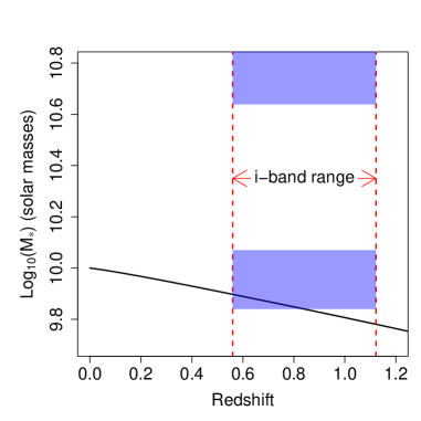
Figure 1: Minimum galaxy mass threshold for inclusion in our data sample as a function of redshift (black solid line), as estimated via the algorithm of Behroozi, Wechsler, & Conroy (2013). In their scheme, if one evolves a sample of galaxies whose masses are all the threshold mass for a particular redshift from that redshift to the present day, the present-day median mass among those galaxies would be $\log_{10}(M_{\ast})\approx 10$. The red dashed lines indicate the redshift boundaries for our data sample: $z\in[0.56,1.122]$. We adopt as a minimum mass the average threshold over this range: $\log_{10}(M_{\rm min})=9.84$. The lower and upper blue rectangles indicate the redshift-mass limits for our low-mass and high-mass quartile samples, respectively. (The upper rectangle is artificially truncated by the plot boundary; in actuality it extends to $\log_{10}(M_{\ast})\approx 12.4$.)

Table 1: Sample size by CANDELS field.

Field	Total	F814W-selected
COSMOS	38 671	704
EGS	41 457	539
GOODSN	35 451	785
UDS	35 932	459
Total	186 441	2487

Our final data sample consists of 2487 galaxies, of which 891 have measured spectroscopic redshifts. Image summary statistics$-$namely, $M,I,D$ (Freeman et al. 2013), $G,M_{20}$ (Abraham, van den Bergh & Nair 2003, Lotz, Primack & Madau 2004), and $C,A$ (Abraham et al. 1994, Abraham et al. 1996a, Abraham et al. 1996b, Conselice 2003)$-$are determined for each galaxy using our own R software suite. (Note that our current definition of the multimode statistic $M$ differs slightly from that of Freeman et al. 2013: we divide the variable $R_{l}$ shown in their equation 1 by the number of pixels in the segmentation map, which places a hard upper limit of 0.5 on the area ratio $R_{l,max}$, achieved when $A_{l,(1)}=A_{l,(2)}=n_{\rm seg}/2$.) We adopt the cataloged star-formation rates estimated by A. Fontana (via “method 6.C,” described in Mobasher et al. 2015).

For the analyses below, we split the data into training and test sets of 1787 and 700 galaxies, respectively. We then assign the smallest and largest 25% of mass (or SFR) values for the training set galaxies to the low-mass (or low-SFR) and high-mass (or high-SFR) groups, respectively.

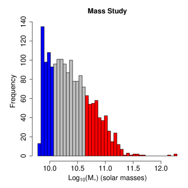
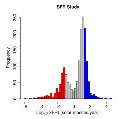
Figure 2: Distributions of masses (top) and star-formation rates (bottom) for the 1787 galaxies in the training set, with the lower and upper quartiles highlighted. Note that the bottom histogram does not include 79 galaxies for which $\widehat{S}=0$ (but which are included in the low-SFR group).

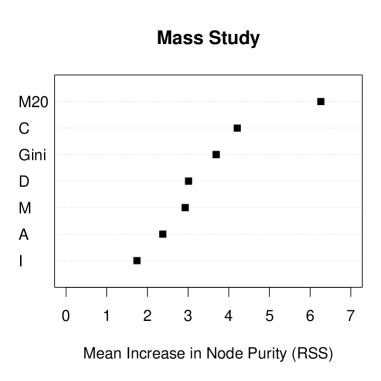
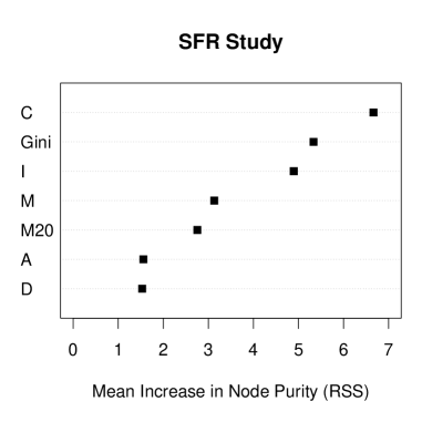
Figure 3: Variable importance measures for random forest regression, as carried out in the morphology-mass study (top panel; Sect. 3.2) and morphology-SFR study (bottom panel; Sect. 3.3). The metric of importance is the mean decrease in the residual sum of squares of the fit that results from splitting the data along the indicated axes. For the mass study, the most important predictor variables ($M_{20}$,$C$,$G$) are all associated with concentration, while for the SFR study the most important variables ($C$,$G$,$I$) are associated with concentration as well as disturbance.

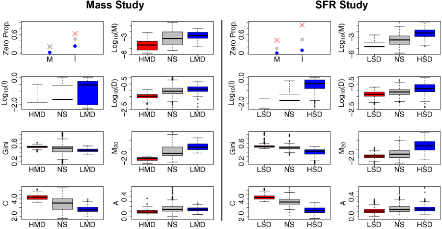
Figure 4: Boxplots summarizing the distributions of each morphological statistic for the morphology-mass study (left bank of panels; Sect. 3.2) and morphology-SFR study (right bank of panels; Sect. 3.3). Within each bank, the leftmost boxplots (red) represent statistics for galaxies identified as being in high-mass-dominated (HMD) or low-SFR-dominated (LSD) regions, the rightmost boxplots (blue) are for galaxies in low-mass-dominated (LMD) or high-SFR-dominated (HSD) regions, and the centre boxplots (grey), labeled “NS” for “not significant,” are for all other galaxies. The top left plot in each bank of panels indicates the proportion of zero values for the $M$ and $I$ statistics, with the same colour scheme as above. We observe that galaxies in HMD/LSD regions are more concentrated and less disturbed than their LMD/HSD region counterparts.

3.2 Morphology-Mass Study

In this study, the predictor and response variables are respectively

• the morphological summary statistics $M$, $I$, $D$, $G$, $M_{20}$, $C$, and $A$; and

• the estimated stellar mass $M_{\ast}=\widehat{M}_{\rm med}$.

We sort the training set masses in ascending order and identify the upper and lower quartiles (see the top panel of Fig. 2). High- and low-mass galaxies are defined as those with log${}_{10}(M)$ $>$ 10.639 and $<$ 10.070 respectively, with the global ratio of low- to high-mass galaxies being unity by definition.

The application of our local two-sample testing algorithm yields the following results for the 700-galaxy test set:

• 108 galaxies are identified as lying in regions of the predictor space where the proportion of high-mass to low-mass galaxies is significantly larger than one, while

• 169 galaxies lie in primarily low-mass regions of predictor space.

In the left panel of Fig. 3 we display variable importances determined by the random forest. These indicate that measures of light concentration ($M_{20}$, $C$, $G$) are more important than measures of disturbance ($D$, $M$, $A$, $I$) for estimating local proportions of high- to low-mass galaxies. This observation is consistent with the boxplots displayed in the left panels of Fig. 4, which show the distributions of individual morphological statistics for galaxies in high-mass-dominated (HMD; red) and low-mass-dominated (LMD; blue) regions, as well as those for galaxies lying where neither class dominates (grey). We observe that galaxies in HMD regions are more concentrated and less disturbed than their counterparts in LMD regions, as one would expect given the redshift range of our sample and previous results regarding “cosmic downsizing” (e.g. Cowie et al. 1996; see also Fig. 7 of Bundy, Ellis & Conselice 2005, which demonstrates at $z\sim 1$ that the fraction of galaxies classified as peculiar decreases as mass increases$-$less disturbance$-$while the fraction of galaxies classified as ellipticals increases with mass$-$greater concentration).

To further visualize how the morphologies of galaxies, and their statistics, change within HMD and LMD regions, we utilize the diffusion map algorithm (Coifman et al. 2005, Coifman & Lafon 2006, Lafon & Lee 2006, Lee & Freeman 2011). Diffusion map is useful for uncovering nonlinear sparse structure in high-dimensional data, including submanifolds, clusters, and high-density regions, etc. We constrast this with e.g. principal components analysis, a linear method wherein data are projected onto hyperplanes. The interested reader can find further general details within the astronomical literature in e.g. Richards et al. (2009) and Freeman et al. (2009), and details on our specific application of diffusion map in Appendix A. The result of our application is to map galaxies from the original seven-dimensional space of morphological statistics to an easily visualized two-dimensional diffusion space. In Fig. 5, we display the first two diffusion coordinates for all 2487 galaxies.

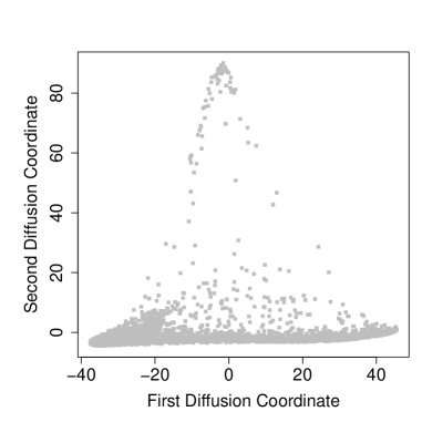
Figure 5: First two diffusion map coordinates resulting from the mapping of the seven-dimensional space of morphological statistics to diffusion space. Each point represents a single galaxy from the the full dataset. See Appendix A for more detail on how one constructs a diffusion map. We stress that in our analysis the goal of using diffusion map is visualization: one should thus not attempt to interpret the absolute numerical values along each axis, which are not readily interpretable. Also, the reader should keep in mind that two-sample testing is performed in the original predictor space and not in diffusion space.

In the top panel of Fig. 6, we retain the diffusion coordinates for the test set data and mark those in HMD and LMD regions using red crosses and blue circles, respectively. We observe a clear separation HMD- and LMD-region galaxies along the first diffusion map coordinate (i.e. from left to right). Galaxies in the HMD region exhibit a consistent appearance$-$concentrated, symmetric, undisturbed$-$with general evidence of discs, while galaxies in the LMD region are generally less concentrated and exhibit a range of appearances due to increased disturbance that becomes more prevalent towards the right. To further quantify these results, we plot the individual statistics of each HMD and LMD region galaxy as a function of principal curve coordinates in the left bank of panels in Fig. 7. Principal curves are smooth one-dimensional curves that provide a one-dimensional summary of multi-dimensional data (Hastie & Stuetzle 1989). In the top left panel of Fig. 7, the principal curves that interpolate the HMD and LMD region galaxies are shown as solid red and blue lines (to the left and right in each panel, respectively). The other panels in the left bank indicate results consistent with those described above: galaxies become progressively less concentrated and more disturbed as one moves from left to right within regions, and across regions.

To assess the consistency of our results with a priori expectation, we construct $UVJ$ and $M_{\ast}$-$UV$ diagrams (Figs. 8 and 9). In the top panel of Fig. 8, quenched galaxies are identified as those that lie above the locus defined by $U-V={\rm max}[1.3,0.88(V-J)+0.59]$ and the vertical line $V-J=1.6$ (Williams et al. 2009). We observe that the majority of galaxies from HMD regions lie on the tight locus of quenched galaxies, as expected. In the top panel of Fig. 9, quenched galaxies lie towards the top (with $U-V$ values $\gtrsim$ 1.3). We observe a positive correlation between being in a HMD region and being quenched, as expected.

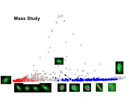
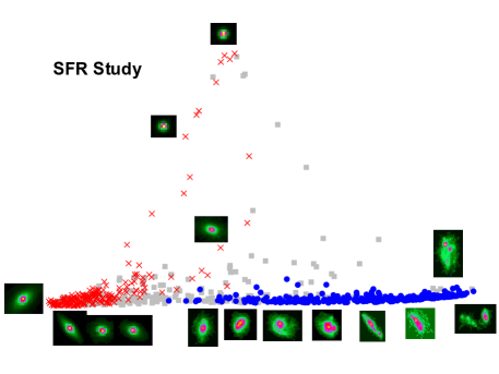
Figure 6: First two diffusion coordinates for the test data for the morphology-mass (top) and morphology-SFR (bottom) studies. Galaxies marked as red crosses are located in regions of the seven-dimensional space of morphological statistics where the local proportion of high-mass (top) or low-SFR (bottom) galaxies is significantly larger than the global proportion, whereas galaxies marked as blue circles reside in low-mass (top) or high-SFR (bottom) regions. There is a clear separation between the regions along the first diffusion coordinate. Representative galaxies are displayed for each group, near their locations in diffusion space. Galaxies to the left exhibit a consistent appearance$-$concentrated, symmetric, undisturbed$-$while the galaxies to the right exhibit increasing amounts of the disturbance.

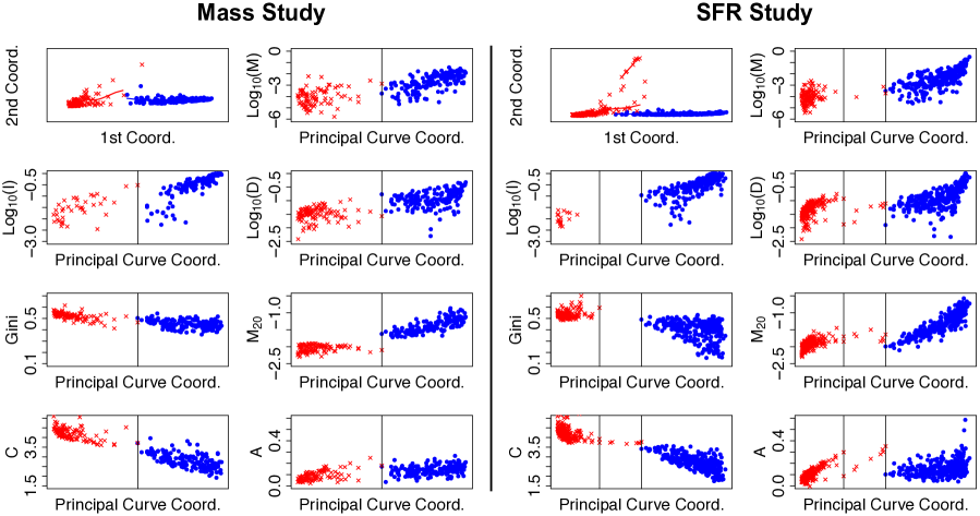
Figure 7: Scatter plots of each morphological statistic as a function of principal curve coordinate for the morphology-mass study (left bank of panels; Sect. 3.2) and morphology-SFR study (right bank of panels; Sect. 3.3). These scatter plots take advantage of the enhanced data visualization afforded by diffusion map to show more detail about the distributions of statistics than the summaries provided by the boxplots in Fig. 4. The top left panel in each bank shows the first two diffusion coordinates for galaxies identified as being in high-mass-dominated (HMD) or low-SFR-dominated (LSD) regions (red crosses, towards the left in each panel), and low-mass-dominated (LMD) or high-SFR-dominated (HSD) regions (blue circles, towards the right), with principal curves for each set of points overlaid. (Note that the red and blue points are the same red and blue points displayed in Fig. 6; we have simply removed the grey points displayed in that figure and decreased the plotting range for the second coordinate to enhance visibility.) In the remaining panels of each bank, the width of each box corresponds to the totality of each principal curve. Note that for the $M$ and $I$ panels, zero values are not displayed (leading to e.g. the absence of points in the middle box of the $I$ panel for the SFR study). The panels in both the left and right banks indicate that galaxies become progressively less concentrated and more disturbed as one move from left to right through the identified regions, as well as across regions.

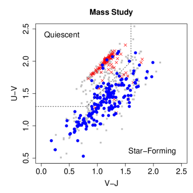
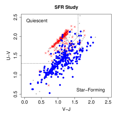
Figure 8: $UVJ$ diagrams for the morphology-mass study (top panel; Sect. 3.2) and morphology-SFR study (bottom panel; Sect. 3.3). In the top panel, galaxies in HMD and LMD regions are shown as red crosses and blue circles, respectively; in the bottom panel, LSD and HSD region galaxies are similarly shown. These diagnostic diagrams show that, consistent with a priori expectation, quenched galaxies largely inhabit a tight locus on the $UVJ$ diagram that lies above the less-tight locus of star-forming galaxies.

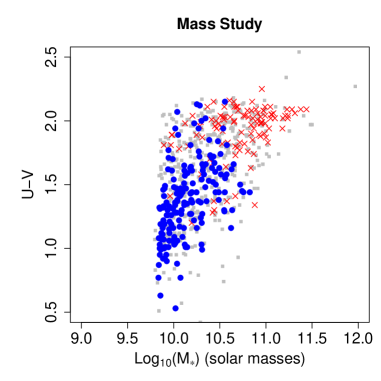
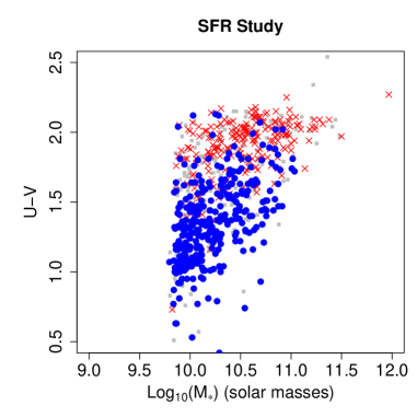
Figure 9: Same as Fig. 8, except that here we plot $U-V$ versus $M_{\ast}$. We observe that low-SFR (i.e. quenched) galaxies are associated with higher mass galaxies.

3.3 Morphology-SFR Study

In this study, the predictor and response variables are respectively

• the morphological summary statistics $M$, $I$, $D$, $G$, $M_{20}$, $C$, and $A$; and

• the estimated star formation rate $S$.

As is the case for the mass study, we sort the training set SFRs in ascending order and define low- and high-SFR galaxies as those with $\log_{10}(S)<-1.01$ and $>1.232$ respectively. (See the bottom panel of Fig. 2.) The application of our two-sample testing algorithm yields that

• 313 of 700 test-set galaxies lie in high-SFR-dominated (HSD) regions, while another

• 214 test-set galaxies lie in low-SFR-dominated (LSD) regions.

In the right panel of Fig. 3, we see that the most important variables for estimating local proportions of high- to low-SFR galaxies are those that measure the concentration of light ($C$ and $G$), although the separation between concentration-related and disturbance-related statistics is not as clear-cut as it is for the mass study. As with the mass study, the boxplots displayed in the right panels of Fig. 4 indicate clear differences between the distributions of summary statistics for each class of galaxy, with galaxies in LSD regions being more concentrated and less disturbed than their counterparts in HSD regions.

In the bottom panel of Fig. 6, we display the first two diffusion map coordinates for the galaxy test-set data, with galaxies in LSD and HSD regions marked as red crosses and blue circles respectively. These regions are largely but not entirely coincident with the HMD and LMD regions shown in the top panel. As is the case for the HMD region, galaxies in the LSD region are concentrated, symmetric, and undisturbed, but in addition to those galaxies that show visual evidence of discs, there are disc-less galaxies, which cluster towards the top of the panel. Conversely, as is the case for the LMD region, galaxies in the HSD region are generally less concentrated and exhibit a range of disturbed morphologies, particularly at the right end of the panel, a high-SFR-dominated but not low-mass-dominated region that is exclusively populated by highly disturbed galaxies that are presumably undergoing mergers. In the right bank of panels in Fig. 7, we show from left to right the galaxy summary statistics for two principal curves fit to LSD region galaxies and one fit to HSD region galaxies. Due to the near-coincidence of the LSD/HSD and HMD/LMD regions, the observed statistic distributions are similar to those in the left bank of panels, but we do note that the HSD region exhibits lower $G$, higher $M_{20}$, and higher $A$ values, etc., than the LMD region, due to the fact that it contains higher numbers of disturbed galaxies.

In Figs. 8 and 9, we show $UVJ$ and $M_{\ast}$-$UV$ diagrams with LSD and HSD regions highlighted. As was the case for the mass study, we observe that the majority of galaxies in LSD regions lie on the locus of quenched galaxies, and that there is a positive correlation between being in a LSD region and being quenched.

Table 2: Assignment of Test Data to Groups

	Low SFR	Not Sig	High SFR	Total
High Mass	78	30	0	108
Not Sig	136	115	172	423
Low Mass	0	28	141	169
Total	214	173	313	700

4 Summary

In this paper, we provide the astronomical community with a local two-sample hypothesis test framework that one can use to more easily analyse data (e.g. morphological statistics, photometric magnitudes, mass and star-formation rate estimates, etc.) in their native high-dimensional spaces. In this framework, one defines two classes based on a response variable of interest (e.g. the top and bottom 25% of the stellar masses for a sample of galaxies), and uses regression to compute the class posterior estimates $\widehat{\mathbb{P}}(Y=y|x)$ given a predictor datum $x$ and where $y$ denotes one of two discrete classes (e.g. high mass in a comparison of high mass and low mass, etc.). We leverage the work of Wager, Hastie & Efron (2014) and Wager & Athey (2015) to convert these estimates to a asymptotically unbiased test statistic that under the null hypothesis converges to a standard normal distribution (eq. 5). In our implementation, we split data into training and test sets, using the former to learn estimates $\widehat{\mathbb{P}}(Y=y|x)$ and generating test statistics at the latter. To mitigate the effect of multiple comparisons (i.e. the fact that the number of tests performed is greater than one), we apply the Benjamini-Hochberg procedure. More details are provided in Algorithm 1 and R-based software is available at github.com/pefreeman/ltst.

Our testing framework has a potential myriad of uses, as it is suitable for use in any analysis situation in which one wishes to test whether a locally estimated proportion of two classes of objects is significantly different from the global proportion. In this paper, we demonstrate the efficacy of our testing framework by applying it to a set of 2487 $i$-band-selected galaxies observed by the HST ACS in the COSMOS, EGS, GOODS-North, and UDS fields. For these galaxies, we compute seven morphological statistics ($M$, $I$, $D$, $G$, $M_{20}$, $C$, $A$) and thus estimate $\mathbb{P}(Y=y|x)$ in this seven-dimensional space. (We note that because our estimation makes use of random forest regression, one can apply our framework to spaces of considerably higher dimensionality. For reference, the computation time for our analyses are $\sim$ 1 CPU minute.) We perform two studies, one in which we determine the local proportion of high-mass (top 25% of masses) to low-mass (bottom 25% of masses) galaxies, and another using star-formation rate in place of mass. Both studies yield qualitatively similar results: galaxies lying in identified high-mass or low-SFR regions exhibit a consistent appearance$-$concentrated, symmetric, undisturbed, and generally with visual evidence of disc structure$-$while their counterparts in low-mass or high-SFR regions have less concentrated light and exhibit increasing levels of disturbance. We display these results first with boxplots (Fig. 4) but then show how one can further potentially visualize results at finer scales by tranforming the predictor data to a lower-dimensional space; here, we specifically apply diffusion map (Figs. 6 and 7). We provide details on diffusion map in Appendix A and R-based software that implements visualization via diffusion map at the address given above.

Appendix A Diffusion Map

Dimensionality reduction methods are useful for visualizing low-dimensional structures embedded in higher-dimensional spaces. One such method is diffusion map (Coifman et al. 2005, Lafon & Lee 2006), a nonlinear method that seeks to preserve the connectivity structure of data within a high-dimensional space. (In practice, preservation means that the Euclidean distance between two points in diffusion space is approximately the same as the sum of all paths between the same two points in the original data space.) The connectivity structure is learned by modeling the traversal of the data space as a diffusion process.

As a starting point for constructing a diffusion map, one defines a weight that reflects the local similarity of two points, $x_{i}$ and $x_{j}$, in $\cal{X}$ = $\{x_{1},\ldots,x_{n}\}$. In this work, we implement the weight estimator of Zelnik-Manor & Perona (2005):

$$\widehat{w}(x_{i},x_{j})=\exp\left(-\frac{s(x_{i},x_{j})^{2}}{\sigma_{i}\sigma_{j}}\right)\,,$$ (6)

where $s$ is the (for example Euclidean) distance between $x_{i}$ and $x_{j}$, and $\sigma_{i}$ ($\sigma_{j}$) is the distance between $x_{i}$ ($x_{j}$) and its $k^{\rm th}$ nearest neighbour. (Note that we standardize the data of each predictor variable first i.e. from each datum we subtract the sample mean and then divide the difference by the sample standard deviation.) We assume $k=30$; other values give similar visualization results. (The appropriate value for $k$ will of course differ from application to application.)

We use the weights $\widehat{w}$ to build a Markov random walk on the data with the transition probability from $x_{i}$ to $x_{j}$ defined as

$$p(x_{i},x_{j})=\frac{\widehat{w}(x_{i},x_{j})}{\sum_{k=1}^{n}\widehat{w}(x_{i},x_{k})}\,.$$ (7)

The one-step transition probabilities are stored in an $n\times n$ matrix $\boldsymbol{P}$, and then propagated by a $t$-step Markov random walk with transition probabilities $\boldsymbol{P}^{t}$. Instead of choosing a fixed time parameter $t$, however, we combine diffusions at all times and define an averaged diffusion map according to

$$\Psi_{\rm av}:x\rightarrow\left[\left(\frac{\lambda_{1}}{1-\lambda_{1}}\right)\psi_{1}(x),\ldots,\left(\frac{\lambda_{m}}{1-\lambda_{m}}\right)\psi_{m}(x)\right]\,,$$ (8)

where $\lambda_{i}$ and $\psi_{i}$ represent the first $m$ eigenvalues and right eigenvectors of $\boldsymbol{P}$. In this work, we fix $m$ to 2, i.e., we only visualize the first two dimensions in diffusion space.

References

- Abraham et al. (1994) Abraham R. G., Valdes F., Yee H. K. C., van den Bergh S., 1994, ApJ, 432, 75
- Abraham et al. (1996a) Abraham R. G., Tanvir N. R., Santiago B. X., Ellis R. S., Glazebrook K., van den Bergh S., 1996a, MNRAS, 279, 47L
- Abraham et al. (1996b) Abraham R. G., van den Bergh S., Glazebrook K., Ellis R. S., Santiago B. X., Surma P., Griffiths R. E., 1996b, ApJS, 107, 1
- Abraham, van den Bergh & Nair (2003) Abraham R. G., van den Bergh S., Nair P., 2003, ApJ, 588, 218
- Barro et al. (2014) Barro G. et al., 2014, ApJ, 791, 52
- Behroozi, Wechsler & Conroy (2013) Behroozi P. S., Wechsler R. H., Conroy C. 2013, ApJ, 770, 57
- Bell et al. (2012) Bell E. F. et al., 2012, ApJ, 753, 167
- Benjamini & Hochberg (1995) Benjamini Y., Hochberg Y., 1995, JRSS B, 57, 289
- Bluck et al. (2014) Bluck A. F. L., Mendel J. T., Ellison S. L., Moreno J., Simard L., Patton D. R., Starkenburg E., 2014, MNRAS, 441, 599
- Bluck et al. (2016) Bluck A. F. L. et al., 2016, MNRAS, 462, 2559
- Brennan et al. (2017) Brennan R. et al., 2017, MNRAS, 465, 619
- Bundy, Ellis & Conselice (2005) Bundy K., Ellis R. S., Conselice C. J., 2005, ApJ, 625, 621
- Coifman & Lafon (2006) Coifman R. R., Lafon S., 2006, ACHA, 21, 5
- Coifman et al. (2005) Coifman R. R., Lafon S., Lee A. B., Maggioni M., Nadler B., Warner F., Zucker S. W., 2005, PNAS, 102, 7426
- Conselice (2003) Conselice C. J., 2003, ApJS, 147, 1
- Conselice (2014) Conselice C. J., 2014, ARA&A, 52, 291
- Cowie et al. (1996) Cowie L. L., Songaila A., Hu E. M., Cohen J. G., 1996, AJ, 112, 839
- Dahlen et al. (2013) Dahlen T. et al., 2013, ApJ, 775, 93
- Duong (2013) Duong T., 2013, JNS, 25, 635
- Elbaz et al. (2011) Elbaz D. et al., 2011, A&A, 533, A119
- Fang et al. (2015) Fang G., Ma Z., Kong X., Fan L., 2015, ApJ, 807, 139
- Freeman et al. (2009) Freeman P. E., Newman J. A., Lee A. B., Richards J. W., Schafer C. M., 2009, MNRAS, 398, 2012
- Freeman et al. (2013) Freeman P. E., Izbicki R., Lee A. B., Newman J. A., Conselice C. J., Koekemoer A. M., Lotz J. M., Mozena M., 2013, MNRAS, 434, 282
- Gretton et al. (2012) Gretton A., Borgwardt K., Rasch M., Schoelkopf B., Smola A., 2012, JMLR, 13, 723
- Grogin et al. (2011) Grogin N. A. et al., 2011, ApJS, 197, 35
- Hastie & Stuetzle (1989) Hastie T., Stuetzle W., 1989, JASA, 84, 502
- Huertas-Company et al. (2016) Huertas-Company M. et al., 2016, MNRAS, 462, 4495
- Koekemoer et al. (2011) Koekemoer A. M. et al., 2011, ApJS, 197, 36
- Lackner & Gunn (2013) Lackner C. N., Gunn J. E., 2013, MNRAS, 428, 2141
- Lafon & Lee (2006) Lafon S., Lee A. B., 2006, IEEE Trans. Pattern Analysis and Machine Intelligence, 28, 1393
- Lang et al. (2014) Lang P. et al., 2014, ApJ, 788, 11
- Lee & Freeman (2011) Lee A. B., Freeman P. E., 2012, in Feigelson E., Babu G., eds., Statistical Challenges in Modern Astronomy V, Springer, New York, p. 255
- Lotz, Primack & Madau (2004) Lotz J. M., Primack J., Madau P., 2004, AJ, 128, 163
- Mobasher et al. (2015) Mobasher B. et al., 2015, ApJ, 808, 101
- Peth et al. (2016) Peth M. A. et al., 2016, MNRAS, 458, 963
- Richards et al. (2009) Richards J. W., Freeman P. E., Lee A. B., Schafer C. M., 2009, ApJ, 691, 32
- Roederer & Hardy (2001) Roederer M., Hardy R. R., 2001, Cytometry, 45, 56
- Salmi et al. (2012) Salmi F., Daddi E., Elbaz D., Sargent M. T., Dickinson M., Renzini A., Bethermin M., Le Borgne D., 2012, ApJ, 754, L14
- Santini et al. (2015) Santini P. et al., 2015, ApJ, 801, 97
- Schaye et al. (2015) Schaye J. et al., 2015, MNRAS, 446, 521
- Sérsic (1963) Sérsic J. L., 1963, BAAA, 6, 41
- Simmons et al. (2017) Simmons B. et al., 2017, MNRAS, 464, 4420
- Snyder et al. (2015) Snyder G. F. et al., 2015, 454, 1886
- Székely & Rizzo (2004) Székely G. J., Rizzo M. L., 2004, InterStat, 5, 1
- Teimoorinia, Bluck & Ellison (2016) Teimoorinia H., Bluck A. F. L, Ellison S. L., 2016, MNRAS, 457, 2086
- Vogelsberger et al. (2014) Vogelsberger M. et al., 2014, MNRAS, 444, 1518
- Wager & Athey (2015) Wager S., Athey S., 2015, arXiv:1510.04342
- Wager, Hastie & Efron (2014) Wager S., Hastie T., Efron B., 2014, JMLR, 15, 1625
- Wake, van Dokkum & Franx (2012) Wake D. A., van Dokkum P. G., Franx M., 2012, ApJ, 751, L44
- Weyant, Schafer & Wood-Vasey (2013) Weyant A., Schafer C., Wood-Vasey W. M., 2013, ApJ, 764, 116
- Williams et al. (2009) Williams R. J., Quadri R. F., Franx M., van Dokkum P., Labbé I., 2009, ApJ, 691, 1879
- Woo et al. (2015) Woo J., Dekel A., Faber S. M., Koo D. C., 2015, MNRAS, 448, 237
- Wuyts et al. (2011) Wuyts S. et al., 2011, ApJ, 742, 96
- Zelnik-Manor & Perona (2005) Zelnik-Manor L., Perona P. 2005, ANIPS, 17, 1601