GLSR-VAE: Geodesic Latent Space Regularization for Variational AutoEncoder Architectures

Abstract

VAEs (Variational AutoEncoders) have proved to be powerful in the context of density modeling and have been used in a variety of contexts for creative purposes. In many settings, the data we model possesses continuous attributes that we would like to take into account at generation time.

We propose in this paper GLSR-VAE, a Geodesic Latent Space Regularization for the Variational AutoEncoder architecture and its generalizations which allows a fine control on the embedding of the data into the latent space. When augmenting the VAE loss with this regularization, changes in the learned latent space reflects changes of the attributes of the data. This deeper understanding of the VAE latent space structure offers the possibility to modulate the attributes of the generated data in a continuous way. We demonstrate its efficiency on a monophonic music generation task where we manage to generate variations of discrete sequences in an intended and playful way.

1 Introduction

Autoencoders [3] are useful for learning to encode observable data into a latent space of smaller dimensionality and thus perform dimensionality reduction (manifold learning). However, the latent variable space often lacks of structure [29] and it is impossible, by construction, to sample from the data distribution. The Variational Autoencoder (VAE) framework [19] addresses these two issues by introducing a regularization on the latent space together with an adapted training procedure. This allows to train complex generative models with latent variables while providing a way to sample from the learned data distribution, which makes it useful for unsupervised density modeling.

Once trained, a VAE provides a decoding function, i.e. a mapping from a low-dimensional latent space to the observation space which defines what is usually called a data manifold (see Fig. 1b). It is interesting to see that, even if the observation space is discrete, the latent variable space is continuous which allows one to define continuous paths in the observation space i.e. images of continuous paths in the latent variable space. This interpolation scheme has been successfully applied to image generation [14, 24] or text generation [4]. However, any continuous path in the latent space can produce an interpolation in the observation space and there is no way to prefer one over another a priori; thus the straight line between two points will not necessary produce the “best” interpolation.

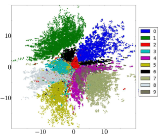
(a) VAE encoding of the MNIST dataset in a latent variable space $\mathcal{Z}:=\mathbf{R}^{2}$. Each point corresponds to a dataset point and colors. Reproduced from [24].

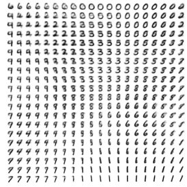
(b) Visualization of the learned data manifold. Reproduced from [19].

Figure 1: Two visualizations of the latent space of a VAE trained on the MNIST dataset.

When dealing with data that contains more information, such as labels or interpretive quantities, it is interesting to see if and how this information has been encoded into the latent space (see Fig. 1a). Understanding the latent space structure can be of great use for the generation of new content as it can provide a way to manipulate high-level concepts in a creative way.

One way to control the generating process on annotated data is by conditioning the VAE model, resulting in the Conditional Variational AutoEncoder (CVAE) architectures [27, 30]. These models can be used to generate images with specific attributes but also allow to generate interpolation between images by changing only a given attribute. In these approaches, the CVAE latent spaces do not contain the high-level information but the randomness of the produced images for fixed attributes.

Another approach, where is no decoupling between the attributes and the latent space representation, consists in finding attribute vectors which are vectors in the latent space that could encode a given high-level feature or concept. Translating an encoded input vector by an attribute vector before decoding it should ideally add an additional attribute to the data. This has been successfully used for image generation with VAEs (coupled with an adversarially learned similarity metric) in [22] and even directly on the high-level feature representation spaces of a classifier [28]. However, these approaches rely on finding a posteriori interpretations of the learned latent space and there is no theoretical reason that simple vector arithmetic has a particular significance in this setting. Indeed, in the original VAE article [19] the MNIST manifold (reproduced in Fig. 1b) has been obtained by transforming a linearly spaced coordinate grid on the unit square through the inverse CDF of the normal distribution in order to obtain “equally-probable” spaces between each decoded image. This advocates for the fact that the latent space coordinates of the data manifold need not be perceived as geodesic normal coordinates. That is, decoding a straight line drawn in the latent space does not give rise to elements whose attributes vary uniformly.

In this work, we focus on fixing a priori the geometry of the latent space when the dataset elements possess continuous (or discrete and ordered) attributes. By introducing a Geodesic Latent Space Regularization (GLSR), we show that it is possible to relate variations in the latent space to variations of the attributes of the decoded elements.

Augmenting the VAE training procedure with a regularizing term has been recently explored in [21] in the context of image generation where the introduction of a discriminative regularization is aimed at improving the visual quality of the samples using a pre-trained classifier. Our approach differs from the one above in the fact that the GLSR favors latent space representations with fixed attribute directions and focuses more on the latent space structure.

We show that adding this regularization grants the latent space a meaningful interpretation while retaining the possibility to sample from the learned data distribution. We demonstrate our claim with experiments on musical data. Our experiments suggest that this regularization also helps to learn latent variable spaces with little correlation between regularized and non regularized dimensions. Adding the possibility to gradually alter a generated sample according to some user-defined criteria can be of great use in many generative tasks. Since decoding is fast, we believe that this technique can be used for interactive and creative purposes in many interesting and novel ways.

2 Regularized Variational Autoencoders

2.1 Background on Variational Autoencoders

We define a Variational AutoEncoder (VAE) as a deep generative model (like Generative Adversarial Networks (GANs) [17]) for observations $x\in\mathcal{X}$ that depends on latent variables $z\in\mathcal{Z}$ by writing the joint distribution $p_{\theta}(x,z)$ as

$$p_{\theta}(x,z)=p(z)p_{\theta}(x|z),$$

where $p(z)$ is a prior distribution over $z$ and $p_{\theta}(x|z)$ a conditional distribution parametrized by a neural network NN$(\theta)$. Given a i.i.d. dataset $X=\{x^{1},\dots,x^{N}\}$ of elements in $\mathcal{X}$, we seek the parameter $\theta$ maximizing the dataset likelihood

$$\log p_{\theta}(X)=\sum_{i=1}^{N}\log p_{\theta}(x^{i}).$$ (1)

However, the marginal probability

$$p_{\theta}(x)=\int p(x,z)\mathrm{d}z$$

and the posterior probability

$$p_{\theta}(z|x)=\frac{p(x,z)}{p(x)}=\frac{p(x,z)}{\int p(x,z)\mathrm{d}z}$$

are generally both computationally intractable which makes maximum likelihood estimation unfeasible. The solution proposed in [19] consists in preforming Variational Inference (VI) by introducing a parametric variational distribution $q_{\phi}(z|x)$ to approximate the model’s posterior distribution and lower-bound the marginal log-likelihood of an observation $x$; this results in:

$$\log p(x)\geq\mathbf{E}_{q_{\phi}(z|x)}\left[\log p(x|z)\right]-D_{KL}(q(z|x)||p(z)):=\mathcal{L}(x;\theta,\phi),$$ (2)

where $D_{KL}$ denotes the Kullback-Leibler divergence [9].

Training is performed by maximizing the Evidence Lower BOund (ELBO) of the dataset

$$\mathcal{L}(\theta,\phi):=\sum_{i=1}^{N}\mathcal{L}(x^{i};\theta,\phi)$$ (3)

by jointly optimizing over the parameters $\theta$ and $\phi$. Depending on the choice of the prior $p(z)$ and of the variational approximation $q_{\phi}(z|x)$, the Kullback-Leibler divergence $D_{KL}(q(z|x)||p(z))$ can either be computed analytically or approximated with Monte Carlo integration.

Eq. (2) can be understood as an autoencoder with stochastic units (first term of $\mathcal{L}(x;\theta,\phi)$) together with a regularization term given by the Kullback-Leibler divergence between the approximation of the posterior and the prior. In this analogy, the distribution $q_{\phi}(z|x)$ plays the role of the encoder network while $p_{\theta}(x|z)$ stands for the decoder network.

2.2 Geodesic Latent Space Regularization (GLSR)

We now suppose that we have access to additional information about the observation space $\mathcal{X}$, namely that it possesses ordered quantities of interest that we want to take into account in our modeling process. These quantities of interest are given as $K$ independent differentiable real attribute functions $\{g_{k}\}$ on $\mathcal{X}$, with $K$ less than the dimension of the latent space.

In order to better understand and visualize what a VAE has learned, it can be interesting to see how the expectations of the attribute functions

$$G_{k}:z\mapsto\mathbf{E}_{p_{\theta}(x|z)}[g_{k}(x)]$$ (4)

behave as functions from $\mathcal{Z}$ to $\mathbf{R}$. In the Information Geometry (IG) literature [2, 1], the $G_{k}$ functions are called the moment parameters of the statistics $g_{k}$.

Contrary to other approaches which try to find attribute vectors or attribute directions a posteriori, we propose to impose the directions of interest in the latent space by linking changes in the latent space $\mathcal{Z}$ to changes of the $G_{k}$ functions at training time. Indeed, linking changes of $G_{k}$ (that have meanings in applications) to changes of the latent variable $z$ is a key point for steering (interactively) generation.

This can be enforced by adding a regularization term over $z=(z_{1},\dots,z_{\textrm{dim}\mathcal{Z}})$ to the ELBO $\mathcal{L(\theta,\phi)}$ of Eq. (3). We define the Geodesic Latent Space Regularization for the Variational Auto-Encoder (GLSR-VAE) by

$$\mathcal{R}_{\textrm{geo}}(z;\{g_{k}\},\theta):=\sum_{k=1}^{K}\mathcal{R}_{k}(z;\theta)$$ (5)

where

$$\mathcal{R}_{k}(z;\theta)=\log r_{k}\left(\frac{\partial G_{k}}{\partial z_{k}}(z)\right).$$ (6)

The distributions $r_{k}$ over the values of the partial derivatives of $G_{k}$ is chosen so that $\mathbf{E}_{u}[r_{k}(u)]>0$, and preferably peaked around its mean value (small variance). Their choice is discussed in appendix B.

Ideally (in the case where the distributions $r_{k}$ are given by Direct delta functions with strictly positive means), this regularization forces infinitesimal changes $\mathrm{d}z_{k}$ of the variable $z$ to be proportional (with a positive factor) to infinitesimal changes of the functions $G_{k}$ (Eq. 4). In this case, for $z_{K+1},\dots,z_{\textrm{dim}\mathcal{Z}}\in\mathcal{Z}$ fixed, the mapping

$$(z_{1},\dots,z_{K})\mapsto(G_{1}(z),\dots,G_{K}(z))\in\mathbf{R}^{K},$$ (7)

where $z=(z_{1},\dots,z_{K},z_{K+1},\dots,z_{\textrm{dim}\mathcal{Z}})$ defines a Euclidean manifold in which geodesics are given by all straight lines.

To summarize, we are maximizing the following regularized ELBO:

$$\mathcal{L}_{\textrm{reg}}(x;\theta,\phi):=\mathbf{E}_{q_{\phi}(z|x)}\left[\log p(x|z)+\mathcal{R}_{\textrm{geo}}(z;\{g_{k}\},\theta)\right]-D_{KL}(q(z|x)||p(z)).$$ (8)

Note that we are taking the expectation of $\mathcal{R_{\textrm{geo}}}$ with respect to the variational distribution $q_{\phi}(z|x)$.

Eq. (8) can be maximized with stochastic gradient ascent using Monte-Carlo estimates of the intractable estimations. We also use the reparametrization trick [19] on stochastic variables to obtain low-variance gradients.

3 Experiments

In this section, we report experiments on training a VAE on the task of modeling the distribution of chorale melodies in the style of J.S. Bach with a geodesic latent space regularization. Learning good latent representations for discrete sequences is known to be a challenging problem with specific issues (compared to the continuous case) as pinpointed in [18]. Sect. 3.1 describes how we used the VAE framework in the context of sequence generation, Sect. 3.2 exposes the dataset we considered and Sect. 3.3 presents experimental results on the influence of the geodesic latent space regularization tailored for a musical application. A more detailed account on our implementation is deferred to appendix A.

3.1 VAEs for Sequence Generation

We focus in this paper on the generation of discrete sequences of a given length using VAEs. Contrary to recent approaches [11, 6, 12], we do not use recurrent latent variable models but encode each entire sequence in a single latent variable.

In this specific case, each sequence $x=(x_{1},\dots,x_{T})\in\mathcal{X}$ is composed of $T$ time steps and has its elements in $[A]$, where $A$ is the number of possible tokens while the variable $z$ is a vector in $\mathcal{Z}$.

We choose the prior $p(z)$ to be a standard Gaussian distribution with zero mean and unit variance.

The approximated posterior or encoder $q_{\phi}(z|x)$ is modeled using a normal distribution $\mathcal{N}(\mu(x),\sigma^{2}(x))$ where the functions $\mu$ and $\sigma^{2}$ are implemented by Recurrent Neural Networks (RNNs) [13].

When modeling the conditional distribution $p_{\theta}(x|z)$ on sequences from $\mathcal{X}$, we suppose that all variables $x_{i}$ are independent, which means that we have the following factorization:

$$p_{\theta}(x|z):=\prod_{i=1}^{T}p_{\theta}^{i}(x_{i}|z).$$ (9)

In order to take into account the sequential aspect of the data and to make our model size independent of the sequence length $T$, we implement $p_{\theta}(x|z)$ using a RNN. The particularity of our implementation is that the latent variable $z$ is only passed as an input of the RNN decoder on the first time step. To enforce this, we introduce a binary mask $m\in\{0,1\}^{T}$ such that $m_{1}=1$ and $m_{i}=0$ for $i>1$ and finally write

$$p_{\theta}(x|z):=\prod_{i=1}^{T}p_{\theta}^{i}(x_{i}|m_{i}*z,m_{<i}),$$ (10)

where the multiplication is a scalar multiplication and where $m_{<i}:=\{m_{1},\dots,m_{i-1}\}$ for $i>1$ and is $\emptyset$ for $i=1$. In practice, this is implemented using one RNN cell which takes as input $m_{i}*z,m_{i}$ and the previous hidden state $h_{i-1}$. The RNN takes also the binary mask itself as an input so that our model differentiates the case $z=0$ from the case where no latent variable is given.

The decoder $p_{\theta}(x|z)$ returns in fact probabilities over $\mathcal{X}$. In order to obtain a sequence in $\mathcal{X}$ we have typically two strategies which are: taking the maximum a posteriori (MAP) sequence

$$x=\textrm{argmax}_{x^{\prime}\in\mathcal{X}}p_{\theta}(x^{\prime}|z)$$ (11)

or sampling each variable independently (because of Eq. (10)). These two strategies give rise to mappings from $\mathcal{Z}$ to $\mathcal{X}$ which are either deterministic (in argmax sampling strategy case) or stochastic. The mapping

$$z\mapsto\textrm{argmax}_{x^{\prime}\in\mathcal{X}}p_{\theta}(x^{\prime}|z)$$ (12)

is usually thought of defining the data manifold learned by a VAE.

Our approach is different from the one proposed in [5] since the latent variable $z$ is only passed on the first time step of the decoder RNN and the variables are independent. We believe that in doing so, we “weaken the decoder” as it is recommended in [5] and force the decoder to use information from latent variable $z$.

We discuss more precisely the parametrization we used for the conditional distribution $p(x|z)$ and the approximated posterior $q(z|x)$ in appendix A.

3.2 Data Preprocessing

We extracted all monophonic soprano parts from the J.S. Bach chorales dataset as given in the music21 [10] Python package. We chose to discretize time with sixteenth notes and used the real name of notes as an encoding. Following [15], we add an extra symbol which encodes that a note is held and not replayed. Every chorale melody is then transposed in all possible keys provided the transposition lies within the original voice ranges. Our dataset is composed of all contiguous subsequences of length $\Delta t=32$ and we use a latent variable space with $12$ dimensions. Our observation space is thus composed of sequences $x=(x_{1},\dots,x_{32})\in\mathcal{X}$ where each element of the sequence $x_{i}$ can be chosen between $A=53$ different tokens.

3.3 Experimental Results

We choose to regularize one dimension by using as a function $g(x):=g_{1}(x)$ the number of played notes in the sequence $x$ (it is an integer which is explicitly given by the representation we use).

3.3.1 Structure of the latent space

Adding this regularization directly influences how the embedding into the latent space is performed by the VAE. We experimentally check that an increase $\Delta z_{1}$ in the first coordinate of the latent space variable $z=(z_{1},\dots,z_{\textrm{dim}\mathcal{Z}})$ leads to an increase of

$$g_{\mathcal{Z}}:=z\mapsto g(\textrm{argmax}(p_{\theta}(x|z))).$$ (13)

The (non-differentiable) function (Eq. 13) is in fact the real quantity of interest, even if it is the the differentiable function $G_{1}$ (Eq. 4) which is involved in the geodesic latent space regularization (Eq. 6). In order to visualize the high-dimensional function $g_{\mathcal{Z}}$, we plot it on a 2-D plane containing the regularized dimension. In the remaining of this article, we always consider the plane

$$P_{z_{1},z_{2}}=\left\{(z_{1},z_{2},0,\dots,0),z_{1},z_{2}\in\mathbf{R}\right\}$$ (14)

Fig. 2 shows plots of the $g_{\mathcal{Z}}$ function restricted to the 2-D plane $P_{z_{1},z_{2}}$. The case where no geodesic latent space regularization is applied is visible in Fig. 2a while the case where the regularization is applied on one latent space dimension is shown in Fig. 2b. There is a clear distinction between both cases: when the regularization is applied, the function $g_{\mathcal{Z}}$ is an increasing function on each horizontal line while there is no predictable pattern or structure in the non-regularized case.

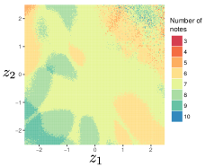
(a) Without geodesic latent space regularization

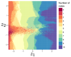
(b) With geodesic latent space regularization

Figure 2: Plot of a 2-D plane in the latent variable space $\mathcal{Z}$. The x-axis corresponds to the regularized dimension.

In order to see if the geodesic latent space regularization has only effects on the regularized quantity (given by $g_{\mathcal{Z}}$) or also affects other (non regularized) attribute functions, we plot as in Fig. 2 these attribute functions (considered as real functions on $\mathcal{Z}$ as in Eq. (13)). Figure 3 show plots of different attribute functions such as the highest and lowest MIDI pitch of the sequence and the presence of sharps or flats. We remark that adding the latent space regularization tends to decorrelate the regularized quantities from the non-regularized ones.

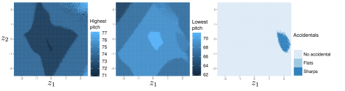
(a) Without geodesic latent space regularization

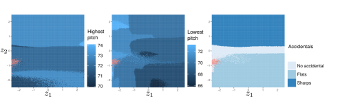
(b) With geodesic latent space regularization

Figure 3: Plot of a 2-D plane in the latent variable space $\mathcal{Z}$. The x-axis corresponds to the regularized dimension. Different non-regularized quantities of the decoded sequences are displayed: the highest pitch, the lowest pitch and if the sequence contains no accidental, sharps or flats.

3.3.2 Generating Variations by moving in the latent space

Reducing correlations between features so that each feature best accounts for only one high-level attribute is often a desired property [7] since it can lead to better generalization and non-redundant representations. This kind of “orthogonal features” is in particular highly suitable for interactive music generation. Indeed, from a musical point of view, it is interesting to be able to generate variations of a given sequence with more notes for instance while the other attributes of the sequence remain unchanged.

The problem of sampling sequences with a fixed number of notes with the correct data distribution has been, for example, addressed in [26] in the context of sequence generation with Markov Chains. In our present case, we have the possibility to progressively add notes to an existing sequence by simply moving with equal steps in the regularized dimension. We show in Fig. 4 how moving only in the regularized dimension of the latent space gives rise to variations of an initial starting sequence in an intended way.

Figure 4: Image of straight line in the data manifold obtained by starting from a random $z$ and then only increasing its first (regularized) coordinate $z_{1}$. The argmax decoding procedure (Eq. 11) was used. All generated sequences are two-bar long and separated by double bar lines. This generates variations of the initial motif by adding more notes.

3.3.3 Effect on the aggregated distribution and validation accuracy

A natural question which arises is: does adding a geodesic regularization on the latent space deteriorates the effect of the Kullback-Leibler regularization or the reconstruction accuracy? The possibility to sample from the data distribution by simply drawing a latent variable $z\sim p(z)$ from the prior distribution and then drawing $x\sim p_{\theta}(x|z)$ from the conditional distribution indeed constitutes one of the great advantage of the VAE architecture.

We check this by looking at the aggregated distribution defined by

$$q_{\phi}(z):=\int_{x}q_{\phi}(z|x)p_{d}(x)\mathrm{d}x,$$ (15)

where $p_{d}(x)$ denotes the data distribution. In an ideal setting, where $q_{\phi}(z|x)$ perfectly matches the posterior $p_{\theta}(z|x)$, the aggregated distribution $q_{\phi}(z)$ should match the prior $p(z)$. We experimentally verify this by plotting the aggregated distribution projected on a 2-D plane in Fig. 5. By assigning colors depending on the regularized quantity, we notice that even if the global aggregated distribution is normally distributed and approach the prior, the aggregated distribution of each cluster of sequences (clustered depending on the number of notes they contain) is not, and depends on the the regularized dimension.

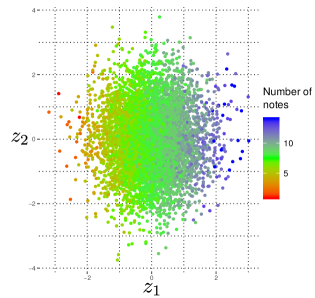
Figure 5: Plot of the aggregated distribution projected on a 2-D plane in the latent space which contains the regularized dimension as its x-axis. Each point is attributed a color depending on the number of notes contained in the decoded sequence.

We report a slight drop (1%) of the reconstruction accuracy when adding the geodesic latent space regularization. The fact that adding a regularization term reduces the reconstruction accuracy has also been noted in [21] where they nonetheless report a better visual quality for their regularized model.

The geodesic latent space regularization thus permits to obtain more meaningful posterior distributions while maintaining the possibility to sample using the prior distribution at the price of a small drop in the reconstruction accuracy. We believe that devising adaptive geodesic latent space regularizations could be a way to prevent this slight deterioration in the model’s performance and provide us with the best of both worlds. Having the possibility to navigate in the latent space seems an important and desired feature for generative models in creative applications.

4 Discussion and Conclusion

In this paper, we introduced a new regularization function on the latent space of a VAE. This geodesic latent space regularization aims at binding a displacement in some directions of the latent space to a qualitative change of the attributes of the decoded sequences. We demonstrated its efficiency on a music generation task by providing a way to generate variations of a given melody in a prescribed way.

Our experiments shows that adding this regularization allows interpolations in the latent space to be more meaningful, gives a notion of geodesic distance to the latent space and provides latent space variables with less correlation between its regularized and non-regularized coordinates.

Future work will aim at generalizing this regularization to variational autoencoders with multiple stochastic layers. It could indeed be a way to tackle the issue of inactive units in the lower stochastic layers as noted in [5, 23], by forcing these lower layers to account for high-level attributes.

Our regularization scheme is general and can be applied to the most recent generalizations of variational autoencoders which introduce generative adversarial training in order to obtain better approximations of the posterior distributions [24, 18] or in order to obtain a better similarity metric [22].

We believe that applying this regularization to conditional VAEs [27, 30] opens up new ways to devise interactive applications in a variety of content generation tasks.

5 Acknowledgments

First author is founded by a PhD scholarship of École Polytechnique (AMX).

Appendix A Implementation Details

We report the specifications for the model used in Sect. 3. All RNNs are implemented as 2-layer stacked LSTMs [16, 25] with 512 units per layer and dropout between layers; we do not find necessary to use more recent regularizations when specifying the non stochastic part model like Zoneout [20] or Recurrent batch normalization [8]. We choose as the probability distribution $r_{1}$ on the partial gradient norm a normal distribution with parameters $\mathcal{N}(2,0.1)$.

We find out that the use of KL annealing was crucial in the training procedure. In order not to let the geodesic latent space regularization too important at the early stages of training, we also introduce an annealing coefficient for this regularization. This means we are maximizing the following regularized ELBO

$$\mathbf{E}_{q_{\phi}(z|x)}\left[\log p(x|z)+\beta\,\mathcal{R}_{\textrm{geo}}(z;\{g_{k}\},\theta)\right]-\beta\,D_{KL}(q(z|x)||p(z))$$ (16)

with $\beta$ slowly varying from $0$ to $1$. We also observe the necessity of early stopping which prevents from overfitting.

Appendix B Choice of the regularization parameters

We highlight in this section the importance of the choice of the regularization distributions $r_{k}$ on the partial gradients (Eq. 6). Typical choices for $r_{k}$ seem to be univariate normal distributions $\mathcal{N}(\mu,\sigma^{2})$ of mean $\mu>0$ and standard deviation $\sigma$.

In practice, this distribution’s mean value must be adapted to the values of the attribute functions $g_{k}$ over the dataset. Its variance must be small enough so that the distribution effectively regularizes the model but high enough so that the model’s performance is not drastically reduced and training still possible. Fig. 6 displays the same figure as in Fig. 2b, but with a regularization distribution $r_{1}$ being a normal distribution $\mathcal{N}(5,1)$. We see that imposing too big an increase to fit in the prior’s range can cause unsuspected effects: we see here a clear separation between two phases.

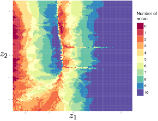
Figure 6: Same plot as in Fig. 2b but with $r_{1}=\mathcal{N}(5,1)$.

What is the best choice for the $r_{k}$ distributions depending on the values of the $g_{k}$ functions over the dataset is an open question we would like to address in future works.

References

- [1] S.-i. Amari. Information geometry and its applications. Springer, 2016.
- [2] S.-i. Amari and H. Nagaoka. Methods of information geometry, volume 191. American Mathematical Soc., 2007.
- [3] Y. Bengio et al. Learning deep architectures for AI. Foundations and trends® in Machine Learning, 2(1):1–127, 2009.
- [4] S. R. Bowman, L. Vilnis, O. Vinyals, A. M. Dai, R. Józefowicz, and S. Bengio. Generating sentences from a continuous space. CoRR, abs/1511.06349, 2015.
- [5] X. Chen, D. P. Kingma, T. Salimans, Y. Duan, P. Dhariwal, J. Schulman, I. Sutskever, and P. Abbeel. Variational lossy autoencoder. arXiv preprint arXiv:1611.02731, 2016.
- [6] J. Chung, K. Kastner, L. Dinh, K. Goel, A. C. Courville, and Y. Bengio. A recurrent latent variable model for sequential data. CoRR, abs/1506.02216, 2015.
- [7] M. Cogswell, F. Ahmed, R. Girshick, L. Zitnick, and D. Batra. Reducing overfitting in deep networks by decorrelating representations. arXiv preprint arXiv:1511.06068, 2015.
- [8] T. Cooijmans, N. Ballas, C. Laurent, Ç. Gülçehre, and A. Courville. Recurrent batch normalization. arXiv preprint arXiv:1603.09025, 2016.
- [9] T. M. Cover and J. A. Thomas. Elements of information theory. John Wiley & Sons, 2012.
- [10] M. S. Cuthbert and C. Ariza. music21: A toolkit for computer-aided musicology and symbolic music data. International Society for Music Information Retrieval, 2010.
- [11] O. Fabius and J. R. van Amersfoort. Variational recurrent auto-encoders. ArXiv e-prints, Dec. 2014.
- [12] M. Fraccaro, S. K. Sønderby, U. Paquet, and O. Winther. Sequential neural models with stochastic layers. In Advances in Neural Information Processing Systems, pages 2199–2207, 2016.
- [13] I. Goodfellow, Y. Bengio, and A. Courville. Deep Learning. MIT Press, 2016. http://www.deeplearningbook.org.
- [14] K. Gregor, I. Danihelka, A. Graves, D. Jimenez Rezende, and D. Wierstra. DRAW: A recurrent neural network for image generation. ArXiv e-prints, Feb. 2015.
- [15] G. Hadjeres, F. Pachet, and F. Nielsen. DeepBach: a steerable model for Bach chorales generation. ArXiv e-prints, Dec. 2016.
- [16] S. Hochreiter and J. Schmidhuber. Long short-term memory. Neural computation, 9(8):1735–1780, 1997.
- [17] Z. Hu, Z. Yang, R. Salakhutdinov, and E. P. Xing. On unifying deep generative models. ArXiv e-prints, June 2017.
- [18] Junbo, Zhao, Y. Kim, K. Zhang, A. M. Rush, and Y. LeCun. Adversarially regularized autoencoders for generating discrete structures. ArXiv e-prints, June 2017.
- [19] D. P. Kingma and M. Welling. Auto-encoding variational Bayes. ArXiv e-prints, Dec. 2013.
- [20] D. Krueger, T. Maharaj, J. Kramár, M. Pezeshki, N. Ballas, N. R. Ke, A. Goyal, Y. Bengio, H. Larochelle, A. Courville, et al. Zoneout: Regularizing rnns by randomly preserving hidden activations. arXiv preprint arXiv:1606.01305, 2016.
- [21] A. Lamb, V. Dumoulin, and A. Courville. Discriminative regularization for generative models. arXiv preprint arXiv:1602.03220, 2016.
- [22] A. B. L. Larsen, S. K. Sønderby, H. Larochelle, and O. Winther. Autoencoding beyond pixels using a learned similarity metric. arXiv preprint arXiv:1512.09300, 2015.
- [23] L. Maaløe, M. Fraccaro, and O. Winther. Semi-supervised generation with cluster-aware generative models. arXiv preprint arXiv:1704.00637, 2017.
- [24] A. Makhzani, J. Shlens, N. Jaitly, I. Goodfellow, and B. Frey. Adversarial autoencoders. arXiv preprint arXiv:1511.05644, 2015.
- [25] T. Mikolov, A. Joulin, S. Chopra, M. Mathieu, and M. Ranzato. Learning longer memory in recurrent neural networks. arXiv preprint arXiv:1412.7753, 2014.
- [26] A. Papadopoulos, P. Roy, and F. Pachet. Assisted lead sheet composition using FlowComposer. In CP, volume 9892 of Lecture Notes in Computer Science, pages 769–785. Springer, 2016.
- [27] K. Sohn, H. Lee, and X. Yan. Learning structured output representation using deep conditional generative models. In C. Cortes, N. D. Lawrence, D. D. Lee, M. Sugiyama, and R. Garnett, editors, Advances in Neural Information Processing Systems 28, pages 3483–3491. Curran Associates, Inc., 2015.
- [28] P. Upchurch, J. Gardner, K. Bala, R. Pless, N. Snavely, and K. Weinberger. Deep feature interpolation for image content changes. arXiv preprint arXiv:1611.05507, 2016.
- [29] P. Vincent, H. Larochelle, I. Lajoie, Y. Bengio, and P.-A. Manzagol. Stacked denoising autoencoders: Learning useful representations in a deep network with a local denoising criterion. Journal of Machine Learning Research, 11(Dec):3371–3408, 2010.
- [30] X. Yan, J. Yang, K. Sohn, and H. Lee. Attribute2Image: Conditional image generation from visual attributes. ArXiv e-prints, Dec. 2015.