An Efficient Approach to Communication-aware Path Planning for Long-range Surveillance Missions undertaken by UAVs

Abstract

While using drones (UAVs) for remote surveillance missions, it is mandatory to do path planning of the vehicle since these are pilot-less vehicles. Path planning, whether offline (more popular) or online, entails setting up the path as a sequence of locations in the 3D Euclidean space, whose coordinates happen to be latitude, longitude and altitude. For the specific application of remote surveillance of long linear infrastructures in non-urban terrain, the continuous 3D-ESP (Euclidean Shortest path) problem practically entails two important scalar costs. The first scalar cost is the distance travelled along the planned path. Since drones are battery operated, hence it is needed that the path length between fixed start and goal locations of a mission should be minimal at all costs. The other scalar cost is the cost of transmitting the acquired video during the mission of remote surveillance, via a camera mounted in the drone’s belly. Because of the length of surveillance target which is long linear infrastructure, the amount of video generated is very high and cannot be generally stored in its entirety, on board. If the connectivity is poor along certain segments of a naive path, to boost video transmission rate, the transmission power of the signal is kept high, which in turn dissipates more battery energy. Hence a path is desired that simultaneously also betters what is known as “communication” cost. These two costs trade-off, and hence Pareto optimization is needed for this 3D biobjective Euclidean shortest path problem. In this report, we study the mono-objective offline path planning problem, based on the distance cost, while posing the communication cost as an upper-bounded constraint. The biobjective path planning solution is presented separately in a companion report.

Chapter 1 Introduction

In recent times, there has been a great demand of UAVs in numerous civil industrial and military operations around the world. UAVs are often deployed for missions that are too ”dull, dirty, or dangerous” for manned aircraft[2]. One of such civilian application of UAVs corresponds to remote surveillance of long linear infrastructures. Such (utility) infrastructures typically include power grids, oil and gas pipelines, railway corridors etc. The area of surveillance for such targets is typically vast, running into tens of kilometers. Hence mission planning for such applications has received separate attention. Other than vastness, such infrastructures also tend to run through complex remote terrains, such as forests, hilly regions, wetlands etc, some of which can be no-fly zones. Such terrains are mostly non-urban. Hence remote surveillance using UAVs has emerged as a cost-effective and efficient solution for monitoring of such infrastructures [3].

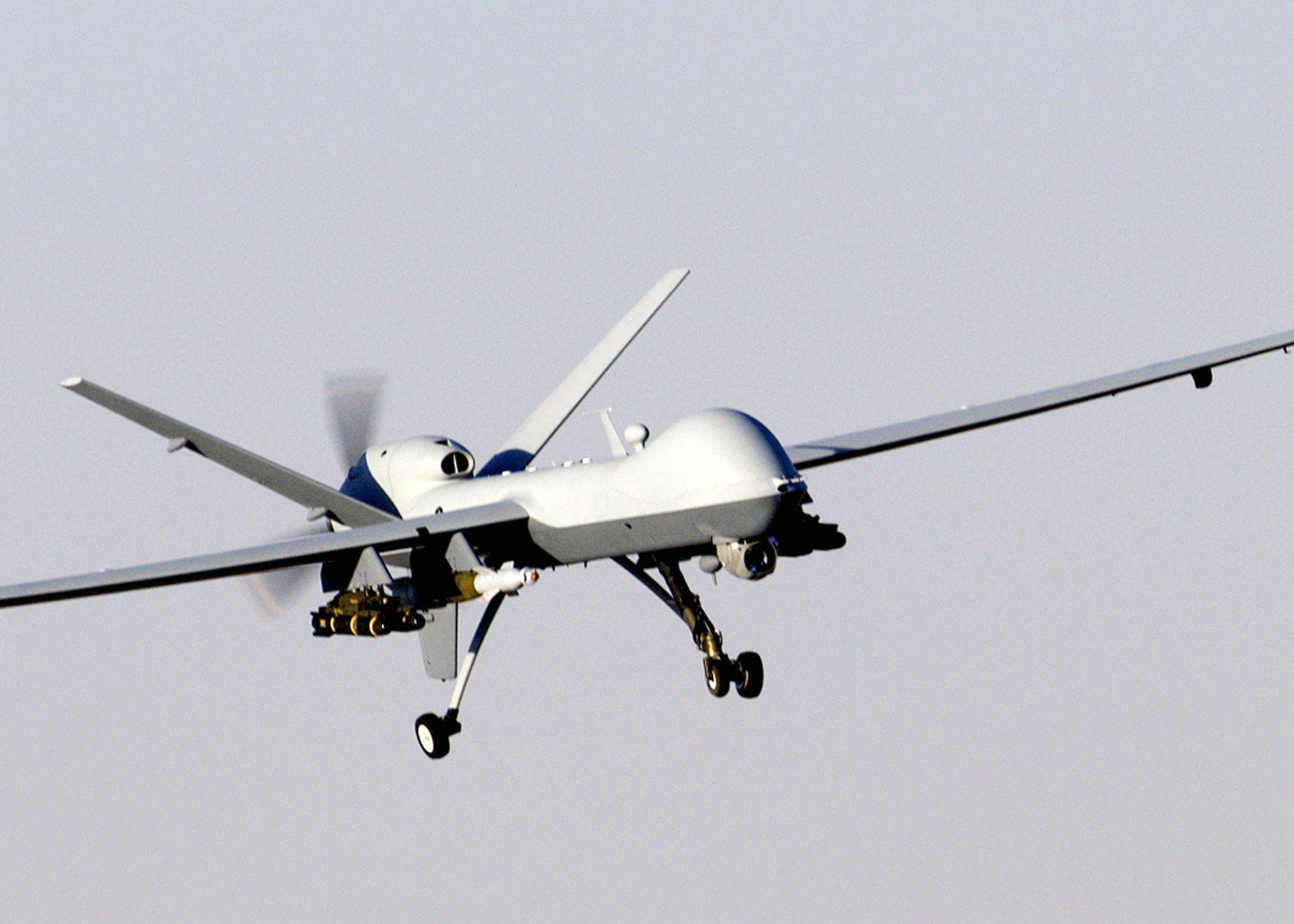
Figure 1.1: An Illustrative Drone in Operation

1.1 Requirement for Live Video Communication

It is imperative that surveillance mission of linear infrastructures results in acquisition of very long and bulky videos. For lack of unlimited storage on-board, or in case of requirement of quick response such as supply breakdown, it is important to transmit the video along the flight. More precisely, often the surveillance video or the sensor data gathered must be transmitted continuously from the UAV to one or more ground control stations (GCS). In disaster and breakdown management, real-time sensor data acquisition and analytics is required to be carried out, before the damage becomes widespread. Further, on long duration flights, which are now quite practical [4], one cannot store entire high volume of video data, typically running in terabytes, and hence needs to transmit it out most of the while. As this data can include urgent high-volume data such as live video, especially in case of long linear infrastructures, maximally uninterrupted high-quality (SNR) connectivity downlink from the UAV to GCS is often required. The required uninterrupted connectivity in remote rural terrain, which may pass through forests, is practically never there. In fact, availability of a carrier by whichever means (RF/Wi-Fi/Public Cellular) is known to be sparse and hence intermittent, in lack of sufficient number of transmitters installed and active in such terrains. Such connectivity can be provided using satellite links, but data rate of such links is well-known to be slow. Hence for such surveillance mission, it makes a lot of sense to perform path planning that additionally factors in the various degrees of available signal coverage, so as to maximize the amount of video transmitted.

1.2 Path Planning as an Optimization Problem

Definition 1.

A path planning algorithm is one that computes a trajectory from the UAV’s present location to a desired future location, e.g. an intermediate or final target[5]. The computation is such that it optimizes certain cost of the path so evolved.

In general, in any space, very large number of solutions/paths exist between a source location and a target/destination location. Sometimes the number of such paths can be countably infinite. However, in reality, we tend to choose paths that suit our specific requirements. These requirements manifest themselves as optimization criteria, entailing certain costs. Hence any such computation of path is done so as to balance various costs attached with executing the mission, e.g. battery power, total distance traveled etc.

Coming to the case of UAVs, path planning of a UAV almost always boils down to optimizing the path length. This is because UAVs are battery operated. Hence, especially for long linear infrastructures, it has always made sense to have a path that can provide maximum-distance/maximum-length coverage of the near-linear/piecewise-linear infrastructural corridor. Such corridors typically have length which can be many times multiple of the maximum path length that a specific battery for a specific class of UAV can offer.

However, as argued earlier, for certain applications, one also needs to maximize connectivity for communication along the same path. This is especially true for the application of remote surveillance of long linear infrastructures. This suggests that the path planning problem could be cast as a biobjective optimization problem, in 3D Euclidean space, for UAVs.

Still, if the path planning is done in a naive, mono-objective fashion for such applications, then it can happen that the UAV may end-up at big-enough coverage hole area. To be able to still ensure that storage for collected/sensed data does not overflow, the UAV will then need to find alternative route, in an online fashion. It is a known fact that any online path planning in a space whose topology is static yields poorer results/cost than offline planning. Thus a naive approach is bound to result in longer mission time. It will also waste valuable battery resource, since algorithm execution consumes power at runtime. Even further, the slowness of algorithm may not allow UAV to fly at its peak speed, since next step has to be decided first before the step is taken by the UAV. Finally, the solution will be poorer since the solution will be locally optimal (finds a detour near obstacle only when the vehicle is close to it), not globally optimal as off-line one. Since the topology of the solution design space is almost completely known a-priori (no-fly zones/obstacles, wireless coverage holes, terrain, surveillance object’s location etc.), off-line design is not only equally possible, but also avoids the above disadvantages of the online algorithm.

On the other hand, if the path planning is done such that both objectives are satisfied to the extent possible together, then in best case, one may be able to get all-time connectivity along the path. If not, even then, one can get good connectivity for most length along the path, which can lead to effective transmission rates most of the while [6]. This not only leads to efficient resource utilization (even signal transmission power is derived from battery power), but also in case of emergency, the report-response time can be minimized.

In this technical report, we provide the design details of an offline heuristic algorithm for path planning with such communication requirement. The path planning problem is tailored for the required surveillance task, and hence favors its deployment on fixed-wing UAVs. However, as can be seen later on, by trivializing the maximum banking angle and minimum route leg length constraints, the same algorithm can also be deployed on commonplace rotary-wing UAVs as well.

Chapter 2 Prior Literature

The prior literature in last few decades till date has mostly focused on traditional path planning. Further, this planning is either agnostic of terrain, or has concerned mainly with Urban areas. Such literature limits itself to consideration of distance covered as cost.

In the plethora of prior works on communication-agnostic path/route planning, A* has been the popular workhorse algorithm, in a discrete navigation space [7]. However, especially for route planning with turning constraints, A* is known to be inefficient [8]. In another solution [9], a graph transformation is performed first, followed by a path search on the transformed graph. But such algorithm is inefficient for simple reason: in a 2D grid for example, there are typically at maximum 1 neighbor left post transform for each node, since the turn limit is generally about 30^∘ [10], [11], [12]. On such a sparse graph, the discretization offset/error is very high. [12] solves this problem using Bellman-Ford algorithm, which is known to have a much higher complexity (O($|$E$|\cdot|$V$|$). In yet another related work [13], angle-constrained motion planning is carried out along with other kinematic constraints arising out of high windy conditions. However, due to dynamic change in the lift, the turn limit itself is a variable. Towards minimization of the alternative aspect of number of turns, few solutions are provided in [14], [2]. However, it is shown that such paths can be up to 22% longer than ideal solution on an average, even in 2D case.

The communication cost has in past been sometimes considered in path planning problems that relate to robotic path/motion planning. In all these works [15], [16], [17], [18], [19], [20], [21], [22], this cost component is modeled as the receiver-end probability of connectivity of the nodes to the base station at all the times, which has to be maximized. Hence this cost is expressed as random variables arising in physical layer function: estimated packet error rate, estimated queue size, at various moments of time. Almost all these works consider multiple robots in action, rather than a single robot, which further involves robots themselves acting as relays. In a single machine case that of a single surveillance UAV, there is no possibility of relaying.

The problem with receiver-end modeling is that the effect of communication channel in between has also to be factored. The wireless communication channel is inherently non-deterministic in terms of its gain. Hence to factor its effect on effective reception rate entails usage of probabilistic, or more precisely, stochastic models.

The main reason behind high degree of uncertainty in reception rate while transmission happens from a moving vehicle is because of multipath effect [20]. Due to multipath, problem is at a short distance from a sampling point in space, the SNR of sampled carrier signal may differ widely [23]. One possibility is to have a very find sampling grid, so that the SNR variation appears gradual when viewed on a discrete graph/grid. However, practically, one cannot do dense sampling for the specific application of ours, given the actual size of the Euclidean space in which path planning has to happen (tens/hundreds of kilometers).

Thankfully, for the application we are interested in, we do not require full-fledged stochastic modeling of the channel. This is because of non-urban, remote terrain, where multipath effects or small-scale fading is almost non-existing. The other two fading components, namely the medium-scale and large-scale fading, can be predicted using deterministic signal propagation modeling, to a good degree of approximation [3]. Online learning of signal quality maps [24] is not worth additional online computation and thus spending some more battery power, since with fixed topology/locations of base stations, and fixed terrain, and quasi-static number of users/quasi-static traffic pattern at a base station, channel characteristics aren’t expected to change heavily with time.

The work in [18] further considers a situation where the information generation rate itself is dynamic and has to be modeled separately, something that does not hold good in our case. Using rough calculations, a fixed, average frame rate such as 30 fps has been found good enough to capture videos that we require, with significant overlap of views captured between two successive frames. Hence, in summary, from prior work [3], we assume a-priori presence of connectivity maps which are assumed to be quasi-stationary.

Also, camera as a visual sensor differs from other sensors in the sense that typically the distance from the object being imaged does not matter, as long as the distance between object and the camera is lesser than camera field of view depth [25]. Hence approaches such as [26] become irrelevant, which take distance between UAV and surveillance object into account. Similarly irrelevant are approaches that plan for moving targets, not just moving remote sensing platform i.e. dynamic coverage [27], [28].

Chapter 3 Problem Restriction

Most real life problems which are modeled and solved mathematically, are first solved in a restricted sense. That is, certain part of details are omitted for various reasons, and the rest of the problem is solved. The details that are ignored must be such that the loss of accuracy of solution can at least be shown to be restricted.

3.1 Restricting Consideration of UAV Motion

The prior work on UAV path planning is mostly organized in two classes. The first class, which views the optimization problem as an optimal flight control problem, retains the details pertaining to the vehicle’s movement. However, it typically abstracts out second-order and higher kinematical effects from the modeling, via a model called Dubin’s vehicle [29]. This class of problem is known as the Motion Planning problem. On the other hand, the second class separates out the vehicle control and optimization concerns. The corresponding optimization problem for the latter concern is known as the Route Planning problem.

It has been provably brought out in [30], [6] that the optimal velocity for each mobile agent is the maximum possible velocity. Further, the cost of such mission is similar to that of a slower-speed mission undertaken by the mobile agent. If we do not exploit this fact, then, in a general setup, a path of any moving system in earth’s gravitational field is a continuous space-time curve obeying the Newtonian laws of motion anyway. Space-time path optimization problems are known to be hard. Hence we ignore time as a variable. but retain location as a (continuous) variable, in the tractable model of path planning. Thus the motion dynamics is ignored in our approach to solution, and we focus on route planning rather. As such, assumption of such constant (maximum) speed decouples the motion and route planning parts of path planning. Similar philosophy is also followed in the popular communication-agnostic 2-phase decoupled trajectory planning approach [7, 31, 32], where the factoring of dynamic constraints is pushed to $2^{nd}$ phase, while focussing on route planning in $1^{st}$ phase. Hence we have currently avoided dealing with Dubin’s path design or motion primitive-based design, towards (direct) motion planning [33].

Even when it comes to route planning, finding an optimal solution is NP-hard, due to presence of obstacles [34]. Hence two philosophical lines of solution exist: combinatorial and sampling-based. Especially in motion planning, randomized sampling based approaches are preferred [31], whenever the solution space is high-dimensional. In the premises of our problem, however, the turn-angle constraint being holonomic, the solution space is practically low-dimensional. Further, we impose five constraints in the overall problem. Hence size of search space becomes quite tractable, along with its low dimensionality. Hence it is more prudent to follow the combinatorial, greedy approach where optimality is not asymptotic, unlike randomized sampling-based algorithms e.g. RRT^∗, PRM^∗, FMT^∗ etc., as described below.

3.2 Restriction against Continuous Optimization

With regard to optimization problems, another important modeling decision has to be taken before the problem model is specified. This decision pertains to modeling the problem as a discrete or continuous optimization problem.

A number of reasons have been cited in various relevant literature, which in a majoritarian way, argue in favor of modeling the problem as a discrete optimization problem. Some of the reasons are

• Even though the number of decision variables are less, the graph size (or more precisely, the size of feasible region), is quite big, given the physical vastness of surveillance area.

• Even if the shortcomings described above could be overcome, any continuous routing model that produces routes having smooth curves probably produces routes that are unflyable by a human pilot or a human UAV controller. Thus, [35] concludes that continuous routing models are unsuitable for use in autorouters.

• Most military applications use Digital Terrain Elevation Data (DTED) as input to their route planners [36], [37]. DTED is grid-based in nature, and hence practically most route planners are anyway grid-based.

• The loss of accuracy in case of discretization is not very high. For the popular route planning algorithm proposed in [38], the shortest paths formed by the edges of 8-neighbor 2D grids are at maximum $\approx$ 8% longer than the shortest paths in the continuous environment. In the same paper, it is further proven that the shortest paths formed by the edges of 26-neighbor 3D grids can at maximum be $\approx$ 13% longer than the shortest paths in the continuous environment.

Discretization has a side effect/disadvantage that any concatenation of straight segments, with only few different angles of possible movement to neighboring cells, in a fixed-topology grid, does not fully utilize the flight capabilities of the air vehicle. For example, in a square/rectangular grid, the theoretically-allowed turns are only restricted to either 45^∘ or 90^∘, to the left or right of the current cell/location. While the shape of grid cell can be changed [39], another possible option is to have a random-topology grid, which is non-uniform, generated by some random process [40]. A very popular non-randomized solution is known as any-angle path planning in a non-random grid. Our solution, as will be detailed later, is derived from that route planning strategy.

Chapter 4 Problem Modeling

Formal specification of any optimization problem entails specification of the decision variables, the cost/objective as a function of these variables, and constraints wherever applicable [41]. For the route planning problem, these parts are detailed as below.

4.1 From Motion Planning to Route Planning

The cameras that are practically used for aerial surveys either do not have multiple frame rates, or cannot be configured dynamically. As such also, there is no need to dynamically change frame rate, since there is sufficient overlap of scene of the remote-surveyed object across successive frames, and there isn’t any need to speed up or slow down the frame rate than typical frame rate either. Once frame rate is fixed, then the other reason why a UAV must speed up or slow down would depend if the sensing and transmitting rates differ (information generation vs information communication rates). Our algorithm is specifically designed in a way that it can handle large communication holes. Hence, once more, there is no specific need to speed up or slow down of UAV during mission either. This leads to constant-speed situation: in which case, one must follow just on the route planning, rather than simultaneously also planning for motion dynamics. Once it comes to this scenario, it is shown in [6] that the best possible UAV speed while simultaneously optimizing for distance and communication costs is the maximum possible speed of the UAV.

If ever one has to do motion planning, then one may still consider [42], [43] algorithms, which do not entail first or higher order dynamical system of equations. Similar is the algorithm Kinematic A* proposed in [44], which goes via offline modeling of speed-dependent movement cost component between two adjacent nodes of the graph. In fact, Dynamic A* algorithm proposed in [45] also follows same philosophy. [10] goes a step further and provides motion planning in wake of a steady-state flow field, typically modeling the wind.

4.2 Decision Variables

There is only one set of decision variables involved. This set is the 3D instantaneous location of the UAV: $\langle x,y,z\rangle$. If the altitude is held/assumed constant, then the location is a 2-tuple, formed by latitude and longitude in world coordinate system. This tuple influences various cost components to be described later, including the sensing cost that we have not considered in this work.

4.3 Constraints

Most of the constraints for the problem are fairly the same across literature, and are rooted in physical control of the unmanned vehicle [46], [47], [48]. We also impose certain constraints on route planning. For more intuition about the constraints, one may refer to [36].

4.3.1 Minimum Route Leg Length

This constraint forces the route to be straight segment, for a predetermined minimum distance, before initiating a turn. Aircraft traveling long distances avoid turning constantly because it adds to pilot fatigue and increases navigational errors. Such constraint generally occurs in conjunction with the turn angle constraint described next.

4.3.2 Maximum Turning Angle

This constraint forces the generated route to make turning manoeuvre, less than or equal to a predetermined maximum turning angle. Such constraint is meant for fixed-wing vehicles, which is what we have assumed for our application. The actual kinematics behind this constraint is explained in [12].

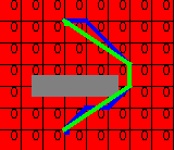
(a)

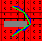
(b)

Figure 4.1: Illustrative Shortest Euclidean Paths with Angle Constraint. Green Line Depicts the Finalized Path

4.3.3 Minimum Separation

This is a very unique constraint for our application. All linear infrastructures, across all nations, require that no man, machine or any other artificial system ever intrude within a pre-specified vicinity of the infrastructure. Such restricted area is called Right of Way. In case of unmanned flight, flying too close to the infrastructure and sudden control failure of the UAV (unmanned vehicles are fairly prone to sudden death) can also mean that the vehicle or a part of it falls on the infrastructure and damages it, which may lead to interruption of the critical supply that that particular infrastructure bears. Further, specifically in the case of power grid corridor, flying too close to HV transmission lines leads to electromagnetic interference between the electrical circuits of the vehicle, and the power line. Such interference has led to corruption of internal flight control data over the internal wires, and eventual failure/dropping dead of few pilot flights for us.

A closely related but separate constraint arises from the fact that at a nominal speed of UAV, and a nominal video frame rate, there is significant overlap between the length of linear infrastructure captured between any two successive frames. This overlap will only reduce if the camera comes closer to the infrastructure. However, the legally enforced constraint of right of way according to us is more sacrosanct, since it relates to system safety. Hence we do not take a minimum of these two lower bounds, but just stick to the right of way constraint only. Overall, from our view, it is of high importance that such a constraint on route design be enforced.

4.3.4 Maximum separation

This is yet another unique constraint arising from the fact that a camera mounted in the belly of the UAV is being used to perform the remote surveillance task. Any visible range digital camera, using any technology has a performance limit, fundamentally due to its usage of lens system, and a finite-sized CCD/CMOS backplane. It is well-proven [25] that if the distance between the object being imaged, and a digital visible-range camera is more than a specific distance known as Depth of Field, then the object cannot be properly imaged/will be as hazy as underlying background, typically earth’s surface/terrestrial terrain. The application demands that the foreground object of interest be reasonably sharp and distinct from background [49], for computer vision techniques to be applied for segmenting out thinner infrastructures against the vast and wide background.

A closely related but separate constraint arises from the fact that certain foreground object of interests e.g. power transmission lines are fairly thin. In such case, to avoid they being imaged at sub-pixel granularity, the camera must stay within a fixed distance from the infrastructure/object at all times.

In summary, once again, from our view, it is of high importance that such a constraint on route design be enforced.

4.3.5 Storage Constraint

This is the third unique constraint arising due to the specific application of ours. Since we are considering communication cost as a component, there are expected to be regions which are no-coverage zones. These regions arise since there is no base station in their vicinity. More specifically, in practical scenarios, most wireless receivers cannot recover signal if the SNR is too low (lower bound). Since there is a single receiver, and single baseband processing unit involved (no MIMO case), SNR thresholding using lower bound implies thresholding of Tx-Rx distance using upper bound (ignoring proportionality constants). In turn, this implies that if closest access point is situated at a distance beyond $d_{minSNR}$, then the UAV is in zero coverage zone. Such a situation can also arise if instead of omni-directional antennas, sector antennas are mounted on the base station.

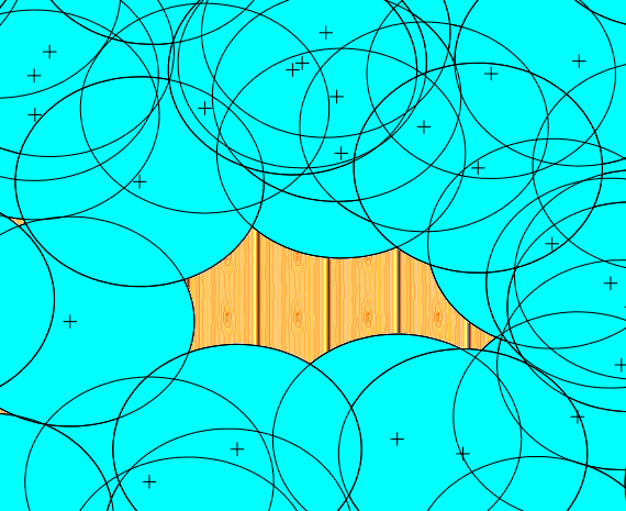
Figure 4.2: A Coverage Hole in Presence of Multiple Receivers

It is not possible to altogether avoid these regions while designing an optimal path. We are having two cost components as described later in this chapter, and these components trade off with each other in a Pareto sense. Hence it is possible that while passing through a zero-coverage zone, the path designed saves a bit on distance cost, while losing a bit on communication cost.

While flying through such regions if the designed route leads to so, we have discussed in section 1.1 that the continuous video being shot has to be stored on-board. The stored video can be transmitted later, when good SNR conditions prevail. However, the storage is not unlimited. If the storage becomes full, then overflow will happen, resulting in a part of video not being available later for any analysis. The filling will happen since the continuous video acquisition leads to terabytes of data generation, while the storage limit would typically be much smaller than that. Since the application of ours mostly deals with fault/damage identification, any missing part in video capture is highly undesired [50]. In order to avoid overflow while storing, one can force the path planning algorithm to only consider options where the segment of the path lying in a specific region has a length that is upper bounded by some constant. This constant (distance) is decided based on the (static) UAV speed, the frame rate of the video camera, the frame size, and the amount of on-board storage. For the entire path, if there are ‘2$\ast$Z’ locations along the path, every successive pair of which implies a zero coverage zone, then

$$\mathbf{\forall i\in\left\{1,\ldots,Z\right\}:\;\|P_{z_{2\cdot i}}-P_{z_{(2\cdot i-1)}}\|\leq d_{zero}}$$

Hence, once again, from our view, it is of high importance that such a constraint on route design be enforced.

4.4 Cost Modeling

As mentioned earlier, we are interested in simultaneously optimizing for two scalar costs. The costs pertain to distance and communication costs. In this report, we have chosen to model only distance cost, and posed the communication cost as an upper-bounded constraint rather. Hence modeling of the communication cost is presented elsewhere, in a companion report on biobjective path planning.

4.4.1 Distance Cost

This cost is a mandatory cost component in all route planning algorithms that have arisen till date. It represents the length, in Euclidean space, of the optimal path undertaken by the vehicle. As is obvious, this cost directly correlates to the limited battery power of the UAV, which are not fuel-driven. At a certain speed of the vehicle, against an assumed constant wind speed, the energy of a charged battery will last only a certain distance. To try maximize the mission, given that application required tens of kilometers to be remotely surveyed, the distance cost has to be minimized. In a discrete graph model of the navigation space, this reduces to finding the shortest path in Euclidean space (Euclidean shortest path). Such problems are fundamental to the area of Computational Geometry!

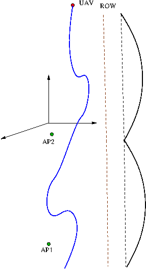
Figure 4.3: A Model for Distance Cost in 2D space. AP represents Communication Access Point.

For any path in discrete grid, piecewise-linear path assumption is valid assumption, also because of $L_{min}$ constraint. In such case, insertion of additional variables to denote the UAV turning points, and sum of Euclidean distances between such successive turning points, is a direct measure of such cost.

Let $P_{T_{i}},i\in 1,\ldots,T$ be the coordinate tuple of each turning point along the path in some coordinate system, e.g. world coordinate system (WCS). Then,

$$\mbox{Path Cost}\;=\;\sum_{i=1}^{T-1}\|P_{T_{i+1}}-P_{T_{i}}\|$$

where $\|\cdot\|$ denotes an appropriate (e.g., L2) norm.

Insertion of additional variables this way implies we also need to add consistency constraints. Observe that the UAV coordinates $\langle x_{U},y_{U},z_{U}\rangle$, do coincide with the coordinates of turning points at certain points in time. Between successive turning points, the UAV coordinates lie on a straight line. If certain pair of successive turning points is within the corridor of flying spanned by ROW (minimum separation) and CDOF (maximum separation) constraints, then all points along the line joining this pair will be obeying these twin constraints automatically. If ALL pairs of successive turning points satisfy ROW and CFOD constraints, the entire path, define as a sequence of UAV position coordinates, will satisfy these twin constraints. Hence we can eliminate variables $x_{U}$, $y_{U}$ and work instead with only coordinates of turning points, $P_{T_{i}}$, to compute this cost component.

4.5 Final Problem Model

minimize
 
$\mbox{~{}~{}~{}~{}~{}~{}~{}~{}~{}}\left[\begin{array}[]{ll}\mbox{({Mandatory})}&\sum\limits_{i=1}^{T-1}\|P_{T_{i+1}}-P_{T_{i}}\|\\ \mbox{(Not used here)}&{\large\oint_{P}}\mathbf{\mbox{~{}~{}min}\left(d_{ap1}^{\alpha},\cdots,d_{apC}^{\alpha}\right)\cdot dp}\end{array}\right]$
 
subject to

$$\mbox{~{}~{}~{}~{}~{}~{}~{}~{}~{}~{}~{}}\|P_{T_{i+1}}-P_{T_{i}}\|\geq L_{min}\mbox{~{}~{}~{}~{}~{}~{}~{}~{}~{}~{}~{}~{}~{}~{}~{}~{}~{}~{}~{}~{}~{}~{}~{}~{}~{}~{}~{}~{}~{}~{}~{}~{}~{}~{}~{}~{}~{}~{}~{}~{}~{}~{}~{}~{}~{}~{}~{}~{}~{}~{}~{}~{}~{}~{}~{}~{}~{}}$$

$$\forall i\in\left\{1,\ldots,T\right\},\forall j\in\left\{1,\ldots,W\right\}\mbox{~{}~{}~{}~{}~{}~{}~{}}y_{P_{T_{i}}}\geq m_{j}\cdot x_{P_{T_{i}}}+c_{j,ROW}$$

$$\forall i\in\left\{1,\ldots,T\right\},\forall j\in\left\{1,\ldots,W\right\}\mbox{~{}~{}~{}~{}~{}~{}}y_{P_{T_{i}}}\leq m_{j}\cdot x_{P_{T_{i}}}+c_{j,CFOD}$$

$$\tan^{-1}\left(\frac{y_{P_{T_{i}}}-y_{P_{T_{i-1}}}}{x_{P_{T_{i}}}-x_{P_{T_{i-1}}}}\right)-\tan^{-1}\left(\frac{y_{P_{T_{i-1}}}-y_{P_{T_{i-2}}}}{x_{P_{T_{i-1}}}-x_{P_{T_{i-2}}}}\right)\leq\theta_{Bmax}\mbox{~{}~{}~{}~{}}$$

$$\forall i\in\left\{1,\ldots,Z\right\}:\;\|P_{z_{2\cdot i}}-P_{z_{(2\cdot i-1)}}\|\leq d_{zero}\mbox{~{}~{}~{}~{}~{}~{}~{}~{}~{}~{}~{}~{}~{}~{}~{}~{}~{}~{}~{}~{}~{}~{}~{}~{}~{}~{}~{}~{}~{}}$$

(Note: Some of the $P_{T_{i}}$ and $P_{z_{i}}$ may coincide in the final solution)  

In the above model, $P_{T_{i}},i\in 1,\ldots,T$ are the coordinate tuple of each turning point along the path in some coordinate system, e.g. world coordinate system. Also, $P_{z_{2\cdot i}}$ and $P_{z_{2\cdot i-1}}$ are successively paired entry and exit points of the desired path in each coverage hole. ROW stands for right of way constraint, and DOF stands for the camera depth of field requirement. The last constraint models the on-board storage limit in a zero-coverage zone (coverage hole).

Chapter 5 Evolutionary Background of Shortest Path Solutions

5.1 Dijkstra’s Algorithm

Dijkstra’s algorithm, along with Bellman-Ford algorithm, is one of the earliest popular solution approach to shortest path problems over discrete graphs. The current popular variant has a fixed single node as the ”source” node, and it finds shortest paths from such source node to all other nodes in the graph, thus producing a shortest-path tree.

Over a graph which has cycles of non-negative cumulative weights, it can be shown that the shortest path problem is in complexity class “P”. Hence optimization techniques such as greedy approach can be used to generate a solution. Dijkstra’s algorithm does exactly that. It starts with source node being the initial node. We presume a notation/definition that the distance of an arbitrary node X be the distance from the initial node to X. Dijkstra’s algorithm assigns some initial distance values to all nodes, and over multiple iterations, tries to greedily improve, in a breadth-first manner, the distance values until they converge. The sketch of steps is as follows.

1. In the initialization step, every node is set to a tentative cost. Most common initialization is zero for initial node, and infinity for all other nodes.

2. First, initial node is marked as current, while all other nodes are marked as unvisited. A set of all the unvisited nodes is created, which may be called the unvisited set.

3. For the current node, all of its unvisited neighbors are checked. Fresh values for their (distance) cost is calculated based on the cost of the partial path till the current node, plus the weight of the edge from the current node to the neighboring node being considered. Such newly calculated tentative cost is compared to the current assigned cost value for each neighbor, and the smaller of the two is assigned as the new cost value for the neighboring node.

4. When all of the neighbors of the current node have been considered, current node is marked/moved to the visited set of nodes, from the unvisited set.

5. Assuming connected graph, which is true in our case, if in any iteration, the destination node has been marked visited , then the algorithm is halted.

6. Otherwise, from the unvisited set, a node that is marked with the smallest tentative cost, is picked up as the new “current node”. Then for next iteration, the algorithm goes back to step (3).

5.2 A* Algorithm

Dijkstra’s algorithm is guaranteed to find a shortest path from the starting point to the goal, as long as none of the edges have a negative cost. However, especially in many real-life applications, there are navigation graphs that contains subgraphs which are forbidden. These forbidden regions typically model some kind of obstacles. Any shortest path algorithm must be able to take this into account and be able to construct a path that circumnavigates the obstacles and yet produce a shortest cost path.

It has been shown that in certain scenarios, an example being when concave obstacle is present in the direct shortest way from source to goal, Dijkstra’s algorithm takes extra time (in terms of amount of partial paths that could have been shortest towards the goal but are killed due to presence of obstacle next to them) to provide the guaranteed solution.

At the other end of the spectrum, one can use best-first local search within the greedy iterations, to improve the cost estimate of the neighboring nodes. For that, such algorithm keeps some estimate (called a heuristic of how far from the goal any vertex is. Instead of selecting the vertex closest to the starting point, as is done in last step of Dijkstra’s algorithm, it selects the vertex closest to the goal. Expectedly, this approach is not guaranteed to find a shortest path. However, it runs much quicker because it an approximate measure called the heuristic function to guide its way towards the goal quickly.

The trouble is this extremal approach is that the algorithm tries to move towards the goal even if it’s not the right path. Since it only considers the cost to get to the goal and ignores the cost of the path so far, it keeps going even if the path it’s on has become really long.

To avoid weak points of both the extremal approaches, A* algorithm was developed in 1968, as a combination of both at local level (path augmentation)[51]. It quantitatively generates the possibilities that a certain direction of path extension along a certain neighbor of the current node is most promising among all neighbors. The algorithm focuses on single-source single-destination, rather than single-source all-destination shortest path of Dijkstra’s. The construction of the shortest path proceeds via the most promising neighbor. At the same time, other neighbors are kept on wait list, so that if the current extending partial path hits a dead end, another promising neighbor with least cost can be picked up a next most promising extension direction, and extension can proceed along with that.

The cost function is modeled as

$$f(n)=g(n)+h(n)$$

Where $g(n)$ is the actual cost from the source node to the current, intermediate node $n$, and $h(n)$ is the estimated cost from the current node $n$ to the goal node. $h(n)$ represents a heuristic estimate. A* finds the best path in shorter time, on an average case, provided that the heuristic function $h(n)$ obeys certain conditions. At each step in the A* path extension, the minimized $f(n)$ value is selected and acted along.

Starting with the source node, the algorithm maintains a priority queue of nodes to be traversed. The lower the value of $f(n)$ for a given node $n$, the higher its priority. At each step of the algorithm, the node with the lowest $f(n)$ value is removed from the queue, the f and g values of its neighbors are updated accordingly, and these neighbors are added to the queue. Note that it is not necessary the selected/removed node is a neighbor of the current node. The algorithm continues until the goal node has a lower f value than any node in the queue. It is possible that the goal node is visited multiple times, since some other partial paths may lead to shorter path to the goal node.

5.2.1 Admissibility Criterion

It has been proved that if the actual cost from any node $n$ to the goal node is $\geq$ estimate $h(n)$, then the A* algorithm is guaranteed to produce a minimum cost path. This condition is known as the admissibility condition.

5.3 Theta* Algorithm

Due to its simplicity and optimality guarantees under admissibility criterion, A* has been, till recently, almost always the search method of choice in real applications. However, in applications in which the environment is continuous (e.g., the UAV navigation in 3D terrain in our case), a shortest path found using A* on any discretized graph is not equivalent to the actual shortest path in the continuous environment. This is because A* constrains paths to be formed by edges of the graph which artificially constrains path headings. The twin figures, borrowed from [1], showcase this gap.

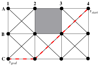
(a) Discrete Shortest Path using Square Grid

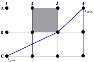
(b) Actual Shortest Path in Continuous Environment

Figure 5.1: Offset between Discrete and Continuous Shortest Paths, courtesy [1]

Many solutions have been proposed for this problem, most of which deal with post-processing of discrete path, to produce a smoother path. However, expectedly, each post-processing technique produces unrealistic results in certain space and/or grid configurations. A recent and quite popular technique which smoothens the path as it is being greedily evolved using A* algorithm, is known as Theta*. It is also known as the Any-Angle Path Planning approach for smoother paths in continuous environments [1].

Theta* is a variant of A* that does not constrain the path being evolved to stick to graph edges. This in turn allows one to try locate any-angle path in the unconstrained continuous environment. It is claimed that the pseudo code for Theta* has only four more lines than the pseudo code for A* and has a similar runtime, but finds path that is nearly identical to the continuous shortest path. The key difference between Theta* and A* is that Theta* allows the parent of a vertex to be any vertex, unlike A* where the parent must be a visible neighbor. To have such extended, transitive parental relation, Theta* updates the g-value and parent of an unexpanded visible neighbor s’ of vertex s by considering the following two paths.

Path 1

As done by A*, Theta* considers the path from the start vertex to s [= g(s)] and from s to s’ in a straight line [= c(s,s’)], resulting in a length of g(s) + c(s,s’).

Path 2

To allow for any-angle paths, Theta* additional considers the grandfatherly path from the start vertex to parent(s) [= g(parent(s))] and from parent(s) to s’ in a straight line [= c(parent(s),s’)], resulting in a length of g(parent(s)) + c(parent(s),s’) if s’ has line-of-sight to parent(s). The idea behind considering this alternative is that in case of Euclidean shortest path problems, this alternative is no longer than previous default path, due to the triangle inequality, if s’ has line-of-sight to parent(s).

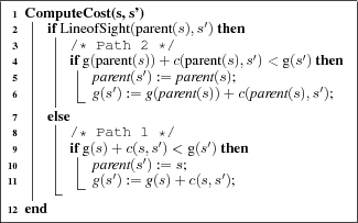
Figure 5.2: Pseudo code for Theta*, courtesy [1]

The additional search logic over A* algorithm is shown in Figure 5.2. We will be using further variation over Theta* algorithm to design an algorithmic solution for our problem.

5.3.1 Variants of Theta*

Due to immense popularity of Theta*, many variations of it have been devised till date. Prominent among them are Pi* [52], Lazy Theta* [38], Angle Propagation Theta*, Augmented Lazy Theta*, Abstract Augmented Lazy Theta* [43] etc. However, most of them deal with reducing the runtime of the algorithm, not exactly changing the logic of the algorithm. At this stage, we are focused on producing better results in terms of path cost offset. Hence we will not be considering these variations at this stage.

Chapter 6 Solution for Mono-objective ESP Problem

To focus on the constraints and hence the feasible set, we first work out a restricted problem involving scalar cost. We choose the popular path/distance cost as the cost to first deal with.

While dealing with this cost, all but one constraints remain practically relevant. The storage constraint, which leads to dealing with zero-coverage zones, is irrelevant for this cost function. However, retaining this constraint does not make the solution illegal or invalid. Hence we retain this constraint here, to understand its impact on the feasible set. In any practical implementation, the designer is free to drop this constraint if required.

6.1 Configuration of Search Space

Before working out the solution to an optimization problem, characterizing the solution is generally done first, to understand what kind of solution/s one can expect. One of the important characterization deals with whether the problem is convex. Convexity of an optimization problem in turn implies convexity of both the underlying set as well as the objective function. These checks can carried out as described in [41].

Coming to a 3D Euclidean space(a set of points in Euclidean space), with obstacles as holes, it is straightforward to see that the underlying set is not convex. To prove this by providing counter-example, take any two points on two sides of the obstacle, when connected via a straight line, will pass through the obstacle. In which case, we cannot claim that points interior to the obstacle and lying on this line are also part of the point set, and the problem becomes non-convex. Hence there is no straightforward characterization of tractability of the problem. In fact, it is proven that for spaces of dimension 3 and above, the problem is NP-hard [34]. Hence approximation algorithms inspired by shortest path algorithms in a convex domain, e.g. Dijkstra, have been researched aplenty.

The Theta* algorithm, which is the basic approximation algorithm that we use, itself gives no guarantee of optimality of the solution, with counter-examples provided to illustrate deviation from optimal solution [1].However, as we show in section 8.4 in detail, Theta* has a marked advantage in terms of computational complexity over the exact algorithms known for solving the 2D ESP problem. Put another way, Theta* trades off some degree of optimality with a marked improvement in computational complexity. Hence we continue/proceed working along their approach. Their approach is also lucrative from the point of view that it allows us to plan the path that is lesser constrained in the angle of turns, thus allowing us to choose within the feasible set with greater freedom for a problem which entails turn angle constraint.

6.2 Discretization of Search Space

We have already discussed in section 3.2 that though the route-planning problem is a continuous optimization problem, we will try solve the discretized version of the problem for various reasons. For discretizing the search space, which happens to be Euclidean, we impose a grid for sampling the space. The grid can be regular based on some pattern, or can be irregular as well. Regular grids are most popularly used in computational geometry, so we will stick to regular grids. Within regular grids, we stick to the pattern which has identical cells. Even further, we assume that the cells are square or cuboid, depending on whether the Euclidean space being considered is 2D or 3D. We call such grid a Uniform Cube Grid. There can be other uniform grids also, for example, one discussed in [53].

6.2.1 Coarseness of Uniform Cube Grid

Given the vast area, running into at least tens of kilometers if not hundreds, that a UAV specific to our application has to cover, we need to decide on the appropriate (constant) cell size. In a similar application discussed in [35], a 200$\times$300 nautical miles area was partitioned into cells having constant size of 8$\times$8 nautical miles. The authors claimed that this spacing corresponds to about one minute of flying time at the typical UAV cruising speed of Mach 0.8. Another reason that the authors have considered is the coarseness of the terrain data made available. The authors had used digital terrain elevation data freely available from the National Geospatial- Intelligence Agency (2004). In that data, elevations are accurate to within $\pm$30 meters at least 90% of the time, and are provided at points on a grid with 1 km spacing. Any grid that is considered hence has to necessarily have dimension units, each of which along a particular Euclidean direction is multiple of the unit size of the DEM grid unit size along the same direction. Thus, for a one minute flight time coarseness, and typical cruising speed and climb and dive rates for their UAVs, they approximated the route-planning grid with vertices that had a two-kilometer horizontal spacing and 200-meter vertical spacing.

If any other kind of map is overlaid on the DEM model, which has to be considered during route planning (e.g. a weather model which predicts position of stormy areas at a particular moment), then the coarseness of that map also has to be taken into account. A composite reference map must have grid size, each of whose dimension which is the minimum of all the overlaid maps [12]. As already mentioned, the route-planning map is a multiple of such composite reference map.

Another useful insight into deciding the grid dimension is provided in [54]. All fixed-wing UAVs have a limit called minimum turning radius. It is imperative the route-planning grid dimension be greater than the turning radius, so that shorter turns get disallowed.

Yet another possibility of fixing grid dimension is to use the minimum route leg length constraint, described in section 4.3.1. The grid dimension can simply be taken to be equal to the constant minimum route leg length. Choice of such grid dimension implies that any straight line path segment, when Theta* algorithm is used, is constrained to be a multiple of the form $(1+\delta)$, where $\delta$ is a positive fractional number. The limitation occurs since $\delta$ is constrained to be from a small finite set of fractional numbers, and cannot be arbitrary (i.e. belonging to infinite set).

Finally, one may note that it is possible to take the world coordinate system (WCS) as the default grid. Sampling of such grid is based on DGPS and altimeter, respectively. A DGPS system gives readings of latitude/longitude with few meters of accuracy. The most common altimeter in form of barometer, which are also most robust altimeters, give reading with accuracy in centimeters. However, hinging the dimension of route-planning grid to such sampling accuracy will lead to very fine grid, something which will make the corresponding discrete graph extremely large in size. This in turn will entail very long path search time. Hence it is important the route-planning grid dimension be decided based on other considerations such as few illustrated earlier.

6.2.2 An Aside on Random Grid

There are certain disadvantages of using regular grids. One of the disadvantage of limited turn angles was highlighted by authors of [1], and solution of that led to solutions that are more close to the optimal solution. On similar lines, in [40], the authors have claimed that if regular grid is used in the Euclidean space, then the banking angle constraints lead to suboptimal solutions over cost function. Hence they suggested that the grid must be irregular, to that there are at least few bigger cells, in which the approximation error of the segment of path passing through them is also relatively smaller. One way of generating an irregular grid, as per their suggestion, is to generate a “space” of randomly length-varying lines, and concatenate them appropriately from source to destination. Then they check various constraints on such concatenations, to drop out infeasible routes. Thus the size of the graph of feasible paths from source to destination shrinks to a smaller feasible set. Over such graph, they propose that one must run any shortest path algorithm with proper non-uniform Euclidean cost edge-weights. However, the cost of generating a random grid for a large side graph adds to the computational complexity of the offline planning software anyway, which is the design tradeoff involved in pursuing this approach.

6.3 Implementing Various Constraints

To search for feasible solution, we first try to locate the feasible set within the appropriate 2D/3D Euclidean space. For certain constraints, it shall be possible to mark out a subspace of the 2D/3D WCS space in which route is physically present, as a union of navigable regions. More precisely, since we discretize the WCS Euclidean space into a grid-based graph, some of the constraints will lead to a bigger feasible set that is a forest. For the remaining constraints, we then greedily search within this forest for either the optimal paths, or just the feasible paths, while simultaneously obeying the remaining constraints during the greedy path formation via stepwise path extension.

6.3.1 Factoring of Feasible Channel Constraints

There are two constraints that lead to direct pruning of the WCS route-planning space. These are the constraints related to minimum separation (c.f. section 4.3.3) and maximum separation (c.f. section 4.3.4).

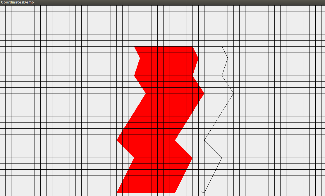
Figure 6.1: A Model of Constrained search space based on separation concerns

(a) A Grid by the side of a Highway

(b) Overlaid Flight Corridor for UAV

Figure 6.2: A Realistic Depiction of Flight Corridor. For brevity, channel is only depicted on one side.

It is straightforward to see that the imposition of minimum separation constraint leads to creation of a half-space on either side of the infrastructure (target of surveillance), that extends till infinity but does not intersect the infrastructure itself. Similarly, it is straightforward to see that the imposition of maximum separation constraint leads to creation of another half-space on either side of the infrastructure. This half space not only extends in the opposite direction that of the half-space arising from minimum separation constraint, but also intersects the infrastructure and does not extend till infinity.

Since our solution has to be such that both constraints are obeyed simultaneously, any such solution necessarily has to lie in the intersection of these two half-space. This in turn means that in 2D case, such intersection is a corridor each on either side of the infrastructure. While in 3D case, it means a cylindrical annuli in which the route must be planned. This pruned search space is depicted in Fig.  6.1.

6.3.2 Factoring of Minimum Route Leg Length Constraint

Minimum route leg length constraint can be taken care in multiple ways. One way is to select a routing grid which has grid dimension same as minimum route leg length, as discussed earlier. In such case, there is nothing to be further taken care of, while searching for an optimal solution. If the grid dimension is not greater than or equal to this constant constraint, then a modification to Theta* is required, wherever a turn is encountered.

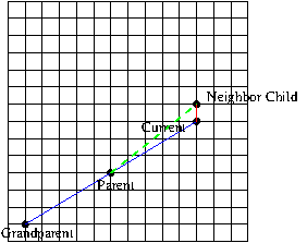
Figure 6.3: Standard Node Nomenclature for Shortest Path Algorithms

Turn is detected necessarily at each path augmentation step, to satisfy the turn constraint that is discussed in next section. To understand how turn is detected at each step, we follow nomenclature shown in Fig. 6.3. We will also use the following theorem as we design our algorithm.

Theorem 1.

In greedy Theta* shortest path algorithm, the direction formed by $\langle$grandparent, parent$\rangle$ and the direction formed by $\langle$parent, current$\rangle$ are not same. That is to say, the nodes grandparent, parent, current are not collinear.

Proof.

We first observe that since the evolving path has already found a path segment between parent node and current node along the line of sight between them, there is no obstacle between them that crosses the line of sight. Similarly, there is no obstacle between grandparent node and parent node that crosses their line of sight. So if these three nodes were collinear, then Theta* algorithm would have found a direct line of sight between grandparent node and current node itself, devoid of any obstacle between them. In which case, parent of current node would have been the grandparent node. Since that is not the case, we have a proof by contradiction that the nodes grandparent, parent, current are indeed not collinear, leading to a turn at parent node. Hence the minimum route leg length would have already been performed between the grandparent node and parent node, by the time the algorithm/path augmentation reaches the current node. Therefore, all one needs to do is that at the current node, while choosing a neighbor to augment the path in best-first way, minimum length check is carried out involving parent node, current node and neighbor/child node, only. ∎

Via this modification, it is first checked that if it is possible to directly join the child node and the parent node, then the distance between them is greater than the minimum route leg length threshold. If it is not so, then following the Theta* logic, alternative indirect path augmentation via current node and then child node may or may not lead to a turning i.e. two possibilities. If the direction between $\langle$parent, current$\rangle$ and the direction between $\langle$current, child$\rangle$ are different, then turn is involved. However, by triangle formed by $\langle$parent, current, child$\rangle$ nodes need not be an obtuse-angled triangle. Hence one must not assume and explicitly check for the distance between $\langle$parent, current$\rangle$ to be greater then the threshold of minimum route length constraint. In the second case, the possible path segment $\langle$parent, current, child$\rangle$ are collinear and hence the constraint must be checked between child node and parent node. If the constraint is not satisfied in the case that is applicable(out of two), then the indirect path augmentation via the current node also fails. In such case, the specific child/neighbor is dropped off consideration, and the next neighboring child must be considered. If none of the neighbors help in obeying the route length constraint, then the algorithm must backtrack, in same way as in handling of the limited-turn-angle constraint, explained next.

6.3.3 Factoring in Angle Constraint

One of the most popular shortest path algorithm remains the A* algorithm, on a discrete grid. However, especially for route planning with turning constraints, A* is known to be inefficient [8]. This is because each of the neighbors, along with path can be possibly extended, leads to turn angle which is constrained to be one of $\langle\pm 45^{\circ},\;\pm 90^{\circ},\;\pm 135^{\circ}\rangle$. This is a highly restricted set to be useful for our application, as explained next.

One possible way of dealing with turn-constrained routing is to perform graph transformation as defined in [9], and doing a path search on the transformed graph. But such algorithm is inefficient for simple reason: in a 2D grid for example, there are typically at maximum 1 neighbor left post transform for each node, since the turn constraint is generally about 30^∘ [10], [11], [12]. On such a sparse graph, the path which is deemed optimal is actually very suboptimal when compared to the optimal path in the continuous version of the problem. Hence we look forward for using any-angle path planning, a group of algorithms proposed under name of “Theta*” [1]. This path search algorithm leads to countably finite but much larger set of feasible turning angles at various points of turn along a path.

A known problem with Theta* algorithm is that at times, it outputs a path that has many turns. A way of minimizing the number of turns is provided in [14], [2]. However, the same paper shows that such paths can be up to 22% more long on an average, in 2D case. In battery-constrained platform such as UAV, such extra cost cannot be afforded. Hence we stick with Theta* only, for the base framework, since it gives much better average case performance (lesser approximation error).

Since there are many scenarios to be considered within modified Theta*, we provide a separate, next section to explain that.

6.4 Angle-Constrained Theta*

6.4.1 Angle Consistency with Grandparent

The first modification within Theta*, over A* algorithm, checks for a line-of-sight condition between the current node’s child/neighbor node, and its parent node. If line of sight exists, then as proved in previous section, due to triangle inequality, the path extended till the child node will make a “turn” at the location of the parent node. The two directions/lines which are involved and subtend a certain turn angle are a) line between current node’s grandparent and the current node’s parent, and b) line between current node’s parent and the current node’s child/neighbor being considered. Hence the first check has to make sure that before current node’s parent and child are connected via a direct path, the above angle is within the limit prescribed by the constraint. If the turn angle is 0^∘, then the constraint is trivially true.

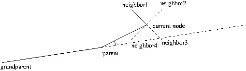
Figure 6.4: Consideration for Turn Constraint in Theta*

6.4.2 Angle Consistency with Parent

If the above angle constraint fails, even if there is a line-of-sight between parent and child of the current node, then one must fall back to the A* way in local sense. In such case, one must check whether the angle subtended between the line from current node’s parent to the current node, and the line from current node to the child being considered, is within the limit prescribed by the constraint. Note that the line between current node’s parent and current node, due to nature of Theta* algorithm, need not be aligned at all with any grid dimension or grid diagonals, since the parent node may be many grid units away from the current node. Hence the possibility of success at this step is also on the higher side, than the possibility considering pure A*. Once again, if the turn angle is 0^∘, then the constraint is trivially true.

6.4.3 Moving on to next Neighbor

If in both of the above cases (considering or not considering triangle inequality), the neighbor node being considered is not found suitable to extend the path along, then we must look for alternatives. In that case, the child node being checked should be dropped from consideration, and another neighbor/child node must be looked for possible and compatible turn constrained path extension.

6.4.4 On Exhaustion of all Neighbors

There are typical scenarios in square grid where plain angle checking involving grandparent, parent, all other neighbors of current node fails, especially around obstacles. In such case, only possible option is to backtrack along the partial path, and try to approach the obstacle using some other neighbor of a prior node on the backtracked path. This leads to a possibility whereby the angle of approach towards a obstacle known/discovered becomes lesser/acute.

Other than obstacles, the algorithm can also fail to extend a partial path through a coverage-dead zone, which behaves like a porous obstacle. As discussed earlier, only few edges are retained across a coverage-dead zone, in the navigation graph/grid. In such case, especially if the approach angle of the partial path towards the boundary of any coverage-dead zone is close to normal, none of the limited edges across such zone may subtend an angle with the approaching partial path which is lesser than the required constrained angle. Hence even if we disregard proper obstacle modeling since it is not required by our application, we still need to design for navigation across/around coverage-dead zone. This, if angle constraints are not getting obeyed, boils down to backtracking and taking a detour.

[55] suggests a heuristics of putting non-uniform weights to the cell, so that any path approaching an obstacle starts gets repulsed to take a detour around the obstacle. [11] suggests another way, which boils down to having an adaptive value of cell size. Our way is different since it involves backtracking in order to circumnavigate the obstacle via alternative route. The direction of turn is immaterial to us, and hence we do not follow any approach similar to [56]. Usage of backtracking in the path evolution is visible in algorithm proposed in [47], albeit in a different way.

To backtrack, it is not necessary that we backtrack all the way to the parent node of the current node. In Theta*, it is possible that the parent node is actually a node very far away from the current node, not necessarily at a distance of unit cell. It is imperative that the farther we backtrack and try approach via a detour, the higher the approximation error become. Hence via a modification to Theta*, we also keep track of which previous node participated in the triangle inequality for the current node. We just go back to that specific neighbor of the current node, and try take a shorter detour when needed. A depiction of such detouring is shown in Fig. 6.5.

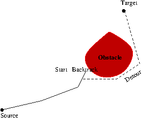
Figure 6.5: Depiction of Unit-step Backtracking and detouring

6.4.5 Factoring of Coverage-dead Zone Constraint

This constraint is intimately related to the storage constraint introduced in section 4.3.5. As discussed there, in order to avoid overflow while storing, one can force the path planning algorithm to only consider options where the segment of the path lying in a specific coverage-dead region to have an upper-bounded length.

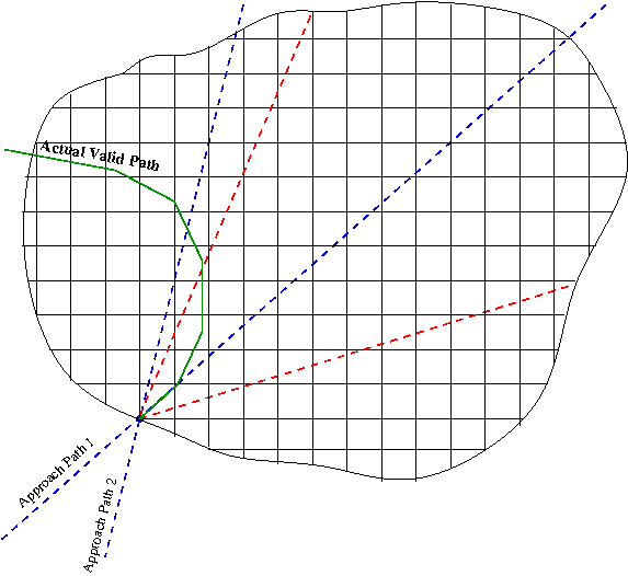
Figure 6.6: Extension of Partial Path using Theta* by Exclusion of Forbidden Sub-zones within Coverage Restricted Zones

Any such path segment has to necessarily cross the coverage-dead zone. In case of A*, a valid path segment crossing the dead zone would have connected two boundary points of the (discretized) dead zone. However, in case of Theta*, neither of the two points of intersection of a valid path with the coverage-dead zone boundary may be a grid point. However, since the path evolves in a greedy fashion, by consideration of one “best” neighboring grid point at a time, what is sure is that any partial path will first intersect any zone’s boundary at a grid point only. It may so happen that after few extensions, the diagonal consideration for path extension using triangle inequality within Theta* may lead to both the entry and exit points of the extended path beyond the coverage-dead zone crosses the zone boundary at fractional grid points. See Fig. 6.6 for an illustration.

Once a partial path arrives at a grid node on the discrete boundary of a coverage-dead zone, its extension within dead zone has to be strictly satisfying the storage constraint i.e. the upper bound on path segment lying within the dead zone. In a naive design, such upper bounded paths are expected to be lying in two sectors formed by a chord of such upper bound length, and the zone boundary. Such sectors are depicted to be to the left and to the right, respectively, of the two red-colored chords of same upper-bound length, in Fig. 6.6. A partial path can arrive at a coverage-dead zone along a direction that when extended can either fall within one of such sector, or it may fall in the remaining dead zone. These two options are depicted via the two blue-colored paths shown in Fig. 6.6.

The presence of such sectors does not rule out the case when a valid path first moves into the sub-zone corresponding to breaching of upper bound, then makes consistent turns into safe sectors/sub-zones and finally exits the dead zone in such a way that overall, the length of extended path segment within the coverage-dead zone is within the upper bound. Such situation is depicted by the green-colored path extension shown in Fig. 6.6. Hence it is clear that any path extension from inside or on the boundary of the dead zone, done in a greedy way, must not be done by imposing the upper bound too early (e.g. via keeping the path extension to be within certain sectors).

It is also desired that the upper-bounded constraint is not imposed once the path is freely extended in a greedy way within the coverage-dead zone, and has just exited the zone. For, if such path has exceeded the upper bound, then one will have to roll back a lot, back to the point of entry of partial path into the dead zone. To be able to still extend path from each current node within the dead zone to one of its neighbors in a constrained way, one can estimate whether any such path extension will lead to violation of the storage constraint.

To check for this violation, at the neighboring point of the current node under consideration, we check if the extension along it will lead to breaching the length upper bound for the path segment lying strictly within the coverage-dead zone. This way, we freely extend the path in the coverage-dead zone, but do not extend it all the way till its exit from the zone. Before we consider a neighbor, we must make a shortlist/subset of neighbors of the current node that satisfy all the remaining constraints. From this shortlist, we consider neighbors one-by-one for extension. For the current node, upper bound cannot be breached, else the path extension would not have reached it. However, if for a particular neighbor, the upper bound is breached, then the path cannot be extended along that neighbor. In such a case, we consider another neighbor from the shortlist and try to extend along that neighbor. If we are unable to extend along any neighbor, then we need to backtrack along the path evolved so far.

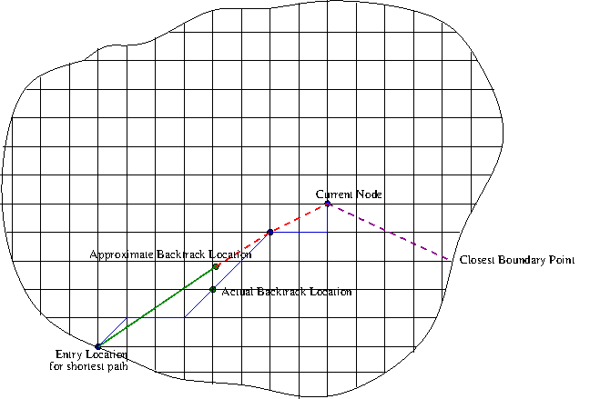
Figure 6.7: Backtracking for Valid Path Extension

How much to backtrack? Must one backtrack all the way to the entry point into the coverage-dead zone, or backtrack just one step back i.e. to the last neighbor of the current node considered by Theta*, or the parent of current node? The answer does not lie in these extremes. Instead, it lies in between. From the current node, one can approximately measure how minimally far one is from the boundary of the coverage-dead zone. This can be measured by taking the distance of the current node from each of the finite boundary points, and taking the minimum. Then, along the path evolved, one must traverse back the same amount of distance, appropriately rounded off to nearest integer. Since such point need not lie on the grid corners, one must locate the nearest grid corner along the path of shortest path evolution. To find such a grid corner, one must consider the two parent nodes (or the parent node and the current node), between which the backtracked point has been marked. The sequence of neighbors considered while evolving path between these two nodes using Theta* is a finite list of grid points which are expected to be closer to the marked location. We take individual distances of the marked location of all these grid points, and pick up the grid point that is closest to marked location. We rescind the path to such closest grid point. All the edges that were previously taken to reach the current node using Theta*, are marked as having infinite weight. From such rescinded grid point, we start our path extension afresh.

For the above backtracking scheme, there will be approximation error in estimation of path rescinding. However, point to note is that we are trying to maximally prune the search space based on whatever exploration we do during the greedy path extension. Also, if we have backtracked enough but not fully, then at some point, after exploring search space from the backtracked point, another backtracking will happen. In such incremental way, we will be able to find a shortest path segment if it exists, if not in fastest possible manner.

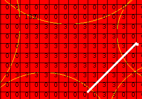
(a) Normal Path Evolution without Backtracking

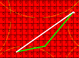
(b) Evolution of Shorter Path involving Backtracking, closer to boundary

Figure 6.8: Illustration of Backtracking within Coverage Hole

6.4.6 Degenerate Cases during Constrained Expansion

So far, we provided details of path expansion design, while satisfying each of the constraints. However, there are specific path extension scenarios, in which the expansion cannot proceed in the straightforward way elaborated so far. In such degenerate scenarios, specific design choices for expansion are made, trading off ease of design with some degree of optimization error.

As first case, it can happen that after finding one better path segment about to grow out of a coverage hole, there exist better path segments passing through the same coverage hole, via the same entry point for the current evolving path. Towards such scenario, whenever a path is entering into a coverage hole, we choose to perform a exhaustive path planning within the entire non-coverage(hole), an induced subgraph of the path planning grid. Even though this increases the computational complexity, it accounts for all the possible paths within the same hole that can be obtained with the same entry point. This in turn avoids re-exploration of the coverage hole in the specific scenario when the head of the currently evolved path has grown beyond the hole, and then due to best-first nature of the algorithm, a node from inside the coverage hole being considered pops up from the heap in the next iteration. If such case happens, then some amount of path planning beyond the coverage hole is discarded. To avoid such wastage, maximal exploration of a coverage hole is done before exiting. This leads to creation of an ”inner“ open list, having the coverage hole entry point and its descendants which are inner nodes. While expanding using this open list, if the path head reaches a boundary node of that coverage hole, path expansion is not allowed to go out of the coverage hole until all other possible exit points, given a fixed entry point of the planned path into that specific coverage hole, are discovered. At the end, only possible exit points remain on the inner open list, and they are merged into the main open list, so that the “best” possible exit option is naturally picked up in the next iteration of (overall) path expansion. One must note that while inner exploration of a specific coverage hole is ongoing using an inner open list, no other sub-paths from outside the hole are allowed to grow (main open list is not considered across iterations). Such design serves a purpose that the entry point into the hole remains same, a requirement that is elaborated as follows. In summary, while exploring a coverage hole for path segments, we do not consider the nodes on the evolved path outside the hole, and vice-versa.

As another case, it can happen that a line-of-sight based merging between neighbor of the current node that is inside a coverage hole, happens to be with parent of the current node that is outside the coverage hole. Such merging will lead to added design complexity, since the entry point of the evolved path into the coverage hole shifts. In turn, the calculated cumulative length so far within coverage hole as described in previous section, becomes incorrect. Also, even if this calculation is corrected one-time, another such merging at later stage of exploration within the coverage hole can lead to re-calculation again. A design option considered here is to fix the path entry point into coverage hole fixed, by forcing the entry point to be a forced parent node to the current node. Thereafter the distance of the current node inside the hole will be checked with reference to this ”forced” parent only.

As a reverse case, it can happen that a line-of-sight based merging between neighbor of the current node that is outside a coverage hole, happens to be with parent of the current node that is inside the coverage hole. Again, the problem with such merging is that the threshold checking done earlier while exploring the coverage hole can get voided, due to shift in the exit node and hence change in the calculation of cumulative length within hole. The proposed solution is very similar to the solution to the previous problem. Here, the exit point of the hole as a boundary point is forced to become a parent node, thus disallowing merging of the above nature. Such design also helps in thwarting the possibility of a line-of-sight based remote merging between two nodes of an evolving path that will intersect a coverage hole that has already been fully explored. Such scenario especially arises when there are multiple holes and multiple obstacles, as will be most practically the case.

Such design of forcing entry and exit nodes of an evolving path to be forced parent node also works in the scenario when an evolving path inside a coverage hole just touches the hole boundary, does not go out and immediately reenters into the same hole. Even though this increases the number of turns in the final path, but it will keep algorithm fail proof and less complex.

As a final case, while doing the path planning the minimum route leg length constraint needs to be checked only when the parent, current and neighbor are non-collinear. If they are collinear, we know that anyway, it came up to that point satisfying the minimum route leg length constraint and addition of one more step in the same direction will not make the constrain to fail. Thus we can avoid a lot of duplicated checking in the algorithm.

6.5 A Note on Migration to Online Path Planning

In previous chapter, we had argued that an off-line path planning algorithm is most suitable for the surveillance application that we are interested in. The terrain and the location of the long linear infrastructure being almost fixed (even in disaster scenario, their components aren’t expected to geolocate themselves significantly), the only reason one would think of doing incremental path planning is when precomputed connectivity map, or SNR map, is unavailable. This can happen sometimes, if an area is not learnt already for its SNR distribution [21]. At other times, along the flight, one gets accurate SNR value, rather than estimated or predicted values, all the time. If the application demands that communication cost be accurate, biobjective online path planning can be thought of. In such case, incremental Pi* algorithm, the online version of basic Theta* algorithm [52], can be modified to meet the requirements of online path planning. This is in line of A* moving to D* and its variants [44] for generic shortest path problems.

One can also plan for a hybrid approach, whereby a gross path is designed off-line, and for each coverage hole, based on continuous SNR observations, path segment within each coverage hole, and till the goal node possibly beyond, is re-planned, once the vehicle enters a coverage hole. In such case, backtracking is no more possible, and mission can fail sometimes. However, if it succeeds, then since the design is based on real, streaming measurement data, the path length is far less pessimistic, and hence one ends up saving on the distance cost as well as communication cost.

Chapter 7 Scaling Mono-objective ESP Solution to 3D Space

So far, we have focussed on path planning in 2D domain, for the ease of understanding. However, in reality, the path of a UAV will be in 3D space. In practice, the change in altitude of the linear infrastructure will not be as vast as change in latitude/longitude of the same, especially if it runs through flat/plateau kind of region. Even then, in theory, the problem is a 3D Euclidean Shortest Path problem.

In continuous domain, 3D path planning problem is known to be NP-hard [57], [46]. Only heuristic and approximate algorithms exist so far for solving such continuous problem. The problem becomes more tractable, once it is discretized. This is one more reason why we turn to discretization of the problem.

Evaluation of suitability of basic Theta* algorithm for 3D UAV path planning, which is also the base algorithm for our solution, was done in [37]. To reduce certain functional ambiguities within Theta*, the paper suggests usage of two gain factors in the cost component functions, $\mathbb{G}$ and $\mathbb{H}$. The paper also introduces a specific constraint for 3D path: the upper bound on rate of climb (altitude-gaining) by UAV, at a given (constant) speed (pitch, yaw, roll something?). More details of this constraint can be found in [54].

While working with 3D discrete ESP, one needs to discretize the altitude direction also. The consideration for discretization of this direction cannot be the same as that of latitude/longitude, described in section 6.2.1. [37] suggests using rate of climb, which is upper-bounded due to capacity of the UAV motors. Once again, in case of an overlaid map such as DEM being used, the resolution of vertical axis in that map must also be factored in.

In case of a 3D discrete grid, any node can have 26 neighbors. Since Theta* does a best-first based expansion, there are scenarios when either multiple neighbors of the same current node, or multiple nodes spaced far apart from each other in the problem space, have same cost value. Which one to choose in best-first way, so that path extension continues from there in an average case (worst case, backtracking happens), is a problem more aptly terms as an ambiguity in [37]. The problem of ambiguity becomes acute due to sheer size of local or semi-local neighborhoods of multiple currents nodes during the iteration for path evolution. To disambiguate, their authors propose using a weighted summation of $\mathbb{H}$ and $\mathbb{G}$, instead of plain summation.

Due to too many iterations in the innermost loop (line-of-sight) check for 3D case, basic theta* becomes computation heavy. Hence a lighter version, more suitable for 3D path planning, called lazy theta* [38] has been worked out.

Since we are considering a unique constraint based on signal strength, the concept of virtual terrain [46] can be used to reduce the problem to 2D. This is because as instantaneous altitude increases for a UAV, the signal strength is only going to grow weak (we have only “base” stations, located on ground). So any optimization algorithm will try pull the path evolution to lowest altitude (especially the heuristic cost function part), as long as the path falls within the 3D annulus of two concentric cylinders. Hence altitude variation will not be much and 3D space can be approximated into a 2D virtual terrain.

7.1 Extending Previous Solution

Many of the strands of previous solution can be scaled directly to the 3D case. It is easy to see that factoring in of feasible channel constraint in 3D space leads to a corridor which is a contiguous sequence of 3D cylindrical annulus, which each element/cylindrical annulus in the sequence representing non-turning/straight segment of the piecewise-linear representation of the infrastructure itself. To see that, one must just rotate the illustration in Fig. 6.1 around the medial line of the winding infrastructure representation. The minimum route leg length constraint checking scales itself trivially, in the Euclidean space via L2 norm way.

The checking for turn angle constraint between two “directions” in 3D space implies the angle formed by them in the 2D-plane that they themselves form (any two lines form a plane in Euclidean and many a non-Euclidean spaces as well). Such an angle can also be decomposed into two angles, one being formed by the projection of two directions on X-Y plane, and the other being formed by the projection of the same directions on either X-Z or Y-Z plane. For most fixed-wing aircrafts, there are different turn angle upper bounds, especially for the altitude direction, hence such decomposition can help them being handled properly at the time of path planning computation. None of the steps for the angle-constrained Theta* variation that we proposed in section 6.4, need to be redesigned for 3D case.

The steps involved in dealing with coverage-dead zone also scale well for 3D case. However, most of the steps become computationally heavy, e.g. finding the minimum distance to the “surface” (instead of perimeter) of a 3D dead zone. The complexity of this computation, and many others, increases by a factor of n. This itself can lead to many backtrackings. Also because of too many ambiguities in choosing the next neighbor as described earlier, there amount of backtrackings can get compounded. A better approach than free-extension-then-backtrack must be designed.

One possibility for that is guided extension within the coverage-dead zone by biasing the cost towards a specific exit boundary point, during the period when the path is evolving within the coverage-dead zone. Such a biasing can ensure that the search for path extension, including backtrackings, are restricted a segment/portion of the coverage-dead zone region. Such a cost bias will be over and atop the bias in path evolution direction that is lent by the heuristic cost component factor, $h(n)$.

Another possibility is to reduce the computational burden by performing only the necessary computations in the base algorithm, Theta*. Such an approach, specifically for 3D path planning, has been evolved by authors of Theta* itself, and is called Lazy Theta* algorithm. Such an approach avoids the trap of not covering the entire path search space within the coverage-dead zone, and yet is computationally lighter than the previous. For more details, refer [38].

Chapter 8 Theoretical Properties of Mono-Objective Solution

Any optimization algorithm, whether exact or approximate, must be checked for correctness of the solution that it provides, ability to find solution when it is shown to exist, and the degree of optimality of the solution generated. In this chapter, we look at each of these properties.

8.1 Correctness

The correctness of a solution to an optimization problem pertains to the solution obeying all the constraints. For the proof that our optimization algorithm is correct, one can easily extend Theorem 1 of [1], and the corresponding Lemma 2, to show that it indeed satisfies all the constraints. We hereby provide the modified statements of the Theorem and the Lemma 2. Their proofs are straightforwards extension of that provided in [1].

Lemma 1.

At any point during the execution of the modified Basic Theta* for our problem, following the parents from any vertex in the open or closed lists to the start vertex retrieves a path that satisfies all the problem constraints enlisted in section 4.5, from the start vertex to this vertex in reverse.

Theorem 2.

When the modified Theta* algorithm terminates, the path extraction retrieves a path satisfying all the problem constraints, from the start vertex to the goal vertex if such a path exists.

The proof for termination of algorithm remains the same as in [1]. The proof for the Lemma can again be made out using induction hypothesis. During each iteration when the current node is extended, and its neighbors expanded, the algorithm ensures that each of the constraint is explicitly satisfied, for at least one neighbor. If in a particular iteration, none of the neighbors can satisfy all the constraints simultaneously, then path extension cannot happen and therefore step-by-step backtracking happens. Eventually, if at least one such path exists, then upon termination of the algorithm, due to comprehensive searching in search space, the algorithm is able to find out one of the optimal paths.

8.2 Completeness

The completeness of a solution to an optimization problem pertains to the algorithm’s ability to find the solution (a constraint-obeying path in our case), if one exists. Again, for the proof that our optimization algorithm is complete, one can easily extend Theorem 1 of [1], and the corresponding Lemma 1. We hereby provide the modified statements of the Theorem and the Lemma 2. Yet again, their proofs are straightforwards extension of that provided in [1].

Lemma 2.

If there exists a (piecewise-continuous) path between any two vertices satisfying all the constraints, then there also exists a grid path (sequence of nodes considered from open list, each of whose neighbors were expanded before the node was put on closed list) between the same two vertices, which was followed/traversed by our modified Theta* algorithm, across iterations, to arrive at the compliant path.

Theorem 3.

The modified Theta* algorithm terminates. If a path satisfying the constraints is known to exist, the algorithm reports one such path upon termination. Else, on termination, the algorithm reports that no such path exists.

The proof for termination of algorithm remains the same as in [1]. The proof of lemma is also straightforward, since in each iteration, we consider a current node and its neighbors. Even if we make a shortcut between the parent of the current node and a neighbor, it can be shown by local induction on the size of the vertex set, that this shortcut can be represented by a sequence of edge mergers. A graph edge necessarily runs between two nodes of a graph. Hence the sequence of edge mergers from one node to another node, leading to formation of an any-angle path, gets represented by a sequence of node traversals.

In the final step to prove the modified theorem, if the algorithm has terminated when its goal vertex has been expanded, then we can use the earlier Lemma 1 to show that the algorithm can output one optimal path. Else, if our algorithm terminates because its open list is empty, then we need to prove that there does not exist any path from the start vertex to the goal vertex, that satisfies all the problem constraints. To prove this statement, we disprove the following contrapositive statement:
If there exists a path satisfying all the problem constraints, from the start vertex to the goal vertex, then our algorithm cannot terminate on the specific condition of its open list of vertices being empty.

The proof of above statement follows the same lines of inductive reasoning, as in [1]. Further, it uses Lemma 2 in the proof. Details of the proof are omitted here for sake of brevity.

8.3 Optimality

The algorithm we have designed is based on Theta* algorithm. As elaborated in [1], Theta* algorithm itself is not an optimal algorithm. It is proved in [38] that any optimal discrete shortest path algorithm, i.e. formed by the edges of 8-neighbor 2D grids can be up to $\approx$ 8% longer than the shortest paths in the continuous environment, in the worst case. Similarly, it is shown that the shortest paths formed by the edges of 26-neighbor 3D grids can be $\approx$ 13% longer than the shortest paths in the continuous environment. The corresponding proofs are non-constructive, thus only giving the bounds but not providing the actual method of constructing such discrete ESPs from scratch. In 2D case, since one can exactly find a continuous ESP using wave propagation algorithm, one can indirectly construct such discrete ESPs as well. For both 2D and 3D scenarios, it is experimentally been shown [58] that in the average case, Theta* typically finds shorter paths than the worst case.

8.4 Computational Complexity

It is known that Dijkstra’s algorithm has a computational complexity of O(E$\cdot\log$V). For a rectangular mesh, if the the number of nodes, —V— = $n$, then the complexity becomes $\equiv$ O($n^{2}\log n$). However, Dijstra’s algorithm computes single source all-target shortest path, i.e. shortest paths to all $n$ nodes. Hence, on an average approximately, the computation it performs to find single-source single-target shortest path is $\approx$ O($n\log n$).

On the other hand, the complexity of A^∗ algorithm is known to be dependent on the heuristic function. In the worst case, the effective branching factor can be too high, leading to exponential complexity overall. However, it is also known that the direct distance heuristic, using Euclidean/L2 norm, is an admissible heuristic. Further, it is known that other than being admissible, the direct distance heuristic leads to expansion of only the nodes that are on the best path, and none else [59]. In such case, the computation complexity becomes equal to the lower bound, i.e. O(d), where $d$ is the length/depth of shortest path. This depth can never be $>$ $n$, and hence the complexity can be approximated as O(n) in the case of direct distance heuristic.

It is further known that if direct distance heuristic is used, then A^∗ algorithm provably finds out the optimal path. With this in mind, we had used direct distance measure as the heuristic when we modified Theta* algorithm. As is already known, Theta* algorithm is essentially A* algorithm with one change for any-angle property. It was shown experimentally in [1] that convergence of Theta* is quite comparable to A*, if not provably. Thus we expect the computational complexity of our algorithm to be $\mathbf{\approx}$ O(n).

8.4.1 Design Tradeoff

To highlight the tradeoff involved, let us examine the set of exact algorithms known for path planning in presence of (polygonal) obstacles. [60], [61] are some of the seminal papers, which provide exact, not approximate solutions to the problem. The runtime of these and many others have been summarized via a table in [62]. It can be seen that while the computational complexity of all these algorithms does not cross O($n\cdot\log n$), it does not fall to O(n) either i.e. is superlinear in $n$. Similarly, for other non-exact approaches, especially easy to program meta-heuristic approaches such as particle swarm and ant colony optimization, relevant texts [63] suggest that their computational complexity is also not linear, but O($n\cdot\log n$).

Against this backdrop, the tradeoff that our algorithm provides becomes clear. We sacrifice a bit on optimality, as discussed in previous section, while we gain on speed. Since we deal with huge graphs (corresponding to area of length tens of miles), the gain in speed is thus significant. The loss in terms of accuracy however is manageable, rather very less, in an average case. Especially when the solution is scaled to more realistic 3D space, where problem is provably NP-hard and only approximate solutions exist, any algorithm with runtime close to O(n) is expected to have a lot of utility value. This gives another compelling reason why we chose the specific design option that led to we choosing to design our approximate, heuristic algorithm.

Chapter 9 Performance Benchmarking

We first experimentally show the efficiency of our algorithm over contemporary ones, for the additional approximation error arising out of circumnavigation of obstacles. With such assurance on practical efficiency of path length, we have more importantly focussed on another performance: the runtime, or convergence performance. This is important since path planning algorithms over vast area, and hence over a mega-sized grid, one must be able to do fast planning, especially in the cases of disaster management where an immediate surveillance mission is most preferred. Even when the search space is low-dimensional as in our case, the sheer volume of space entails fast planning efforts.

To the best of our knowledge, no research work exists that considers coverage holes during path planning as well. Hence it is not possible to do a direct comparison with performance of existing algorithms. We however, still performed three comparisons.

9.1 Performance Degradation due to Incorporation of Extra Constraints

As mentioned earlier, we modified Theta* algorithm so that greedy path evolution proceeds while satisfying four extra constraints. Due to extra computation, it is imperative that the modified algorithm runs slower than Theta*. In one test, we tried to check, using multiple test cases, how much slower the algorithm becomes, assuming same source and goal nodes, and same placement and topology of obstacles (Theta* does not give special treatment to coverage holes).

It was found that on an average across multiple test cases, the slowdown was about 2x-3x. On the positive side, despite such slowdown, our algorithm does provide a more real solution than Theta*, in a more real scenario for UAV path planning. To recall that Theta* was designed for 2D gaming scenario, when much of these constraints are not applicable.

9.2 Cost Comparison for Single Constraint

Again, to the best of our knowledge, no research work exists that combines greedy backtracking with greedy path augmentation (Theta*), for just the turn-angle constraint only. Hence a direct comparison with runtime performance of existing algorithms is at most crude. Still, a short semi-analytical comparison with repulsion-based angle-constrained path planning [55] is discussed below.

9.2.1 Repulsion versus Backtracking

As mentioned before, [55] suggests a heuristics of putting non-uniform weights to the cell, so that any path approaching an obstacle starts gets repulsed to take a detour around the obstacle. [11] implements this suggestion by providing a formal way to specify this repulsion “field”. One major disadvantage of this algorithm is that the set of non-uniform weights around each obstacle is dependent on the topology of the region that the obstacle represents. For example, for a concave obstacle, due to turn angle constraint, one will need to model repulsion from a farther distance than a convex obstacle of same size. Similarly, the size of obstacle is another parameter that will impact the design of obstacle-specific repulsion “field” around it. Our algorithm requires no such heavy preprocessing. Further, our algorithm does efficient, locally minimal backtracking by design.

Unlike our algorithm, [55] only proposes putting a repulsion “field” around each obstacle, and does not guarantee that it is of minimal size. For a quick numerical comparison, we downloaded and used the same dataset as used in [11], the OpenStreetMaps (OSM) dataset. We chose to only compare the relative path length and success rate as parameters, against the LIAN-5 algorithm therein (the fastest among the LIAN family). The relative path length is measured as a fraction against the direct line-of-sight distance between the source and the goal node. We chose 30 rectangular fragments in which length is few orders more than the width (size 1950m x 315m). We discretized the grid with a square cell of size 3m x 3m, as the unit cell. Like [11], we also marked cells corresponding to the areas occupied by buildings as un-traversable. We randomly chose source and goal nodes in each fragment such that the LOS distance is at least 1500m. The angle limit, $\theta_{Bmax}$, was set to 20^∘. As can be seen from table  9.1, the discretization error of 6% is within the limit of 8%, established earlier. At the very least, this comparison is able to point towards more closeness of our approach, to the optimal solution, than a very recent approach. Also, we are able to find a path in almost all cases, since our algorithm can backtrack, and hence is able to span most of the solution space.

Table 9.1: Cost Comparison of LIAN-5 and our Algorithm

	$\theta_{Bmax}$ = 20∘
	success rate	relative path length
LIAN-5	87%	1.14
Our Algorithm	98%	1.06

9.3 Comparing Performance with Brute-force Path Planning

At one extreme, we have our algorithm that prunes the feasible set of solutions in a greedy way, and converges fast to an approximate solution. At the other extreme, we can brute-force enumerate all the solutions within the feasible set, and then check how many iterations it takes during the enumeration, on an average across multiple enumerations/test cases, before we locate an optimal solution. Obviously, a lot depends on how the enumeration is performed. If we perform the enumeration in some efficient way, then comparing the performance of our algorithm to such efficient brute-force solution-finding algorithm leads to establishment of best-case relative performance of our algorithm. Such relative performance, in turn, gives a pessimistic lower bound to our algorithm, and actual performance is expected to be better than that figure of merit.

9.3.1 Algorithm for Brute Force Path Planning

This algorithm is a small improvement over planning algorithm of [8]. We model our brute-force path planning algorithm on the lines of intuitive limited backtracking as described in section 6.4.5. We do not perform the most naive way of brute force path planning, that is, evolving each path independently, end-to-end, and then testing each of them for being compliant to the conditions of our problem. We avoid doing that so that we can have a more realistic comparison (average case performance gain as against worst case performance gain). Similarly, to compare one variety of apple with another variety of apple, not orange, we use Theta* to evolve brute force path during each iteration of brute force algorithm.

We first use basic Theta* to find a path from source node to goal node, that does not cross any obstacle. Next, we trace the solution path from source node to goal node, and at each intermediate node, check for all four constraints that are specific to our problem. If at a certain intermediate node, if one or more constraints are found to be violated, we start the search for the next optimal solution in its vicinity. That is, the sequence of nodes in current path from source till some node in vicinity of the specific intermediate node are retained in the same sequence, certain nodes immediately following the intermediate node in the current path blocked out, and alternative, remaining neighbors to the current node are re-explored to find another optimal path in certain scenarios. Which node to backtrack to, so that nodes from source till the backtracked node are retained, is explained below.

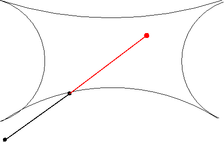
(a) Failure while previous turn is outside

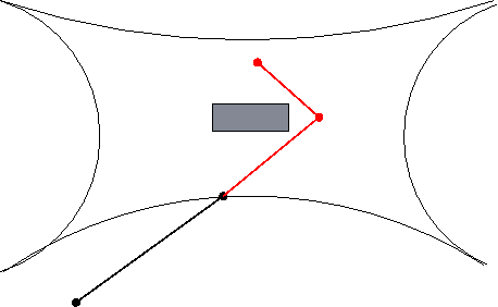
(b) Failure while previous turn is inside

Figure 9.1: Failure of Coverage Hole Storage Constraint

To locate a node where one of the multiple constraints is failing, we need to test for compliance of each constraint at each node in the current path, in some priority order. The priority order, chosen intuitively in decreasing fashion, is maximum storage constraint (c.f. section 4.3.5) followed by maximum turning angle constraint (c.f. section 4.3.2) followed by minimum route length constraint (c.f. section 4.3.1). The first check, that of storage constraint within coverage hole, can fail in two ways, as discussed in the Fig. 9.1. In the first case, there exists no turn between the node of failure for storage constraint, and the node for entry into that specific hole, in the current path. In the second case, a turn exists between the same two above-mentioned nodes. Both of these failure cases need to be treated separately. In the first case, the entire line segment up to the node of failure in the coverage hole need to be stored in a separate “to be blocked” list, whose reason is explained in section 9.3.1. Further, the evolution of next path backtracks to the entry node on boundary of the current coverage hole, and resumes from there. In the latter case, the backtracking needs to happen only up to the previous turn (parent node to the node of failure). From there, evolution of next path will resume, blocking all the nodes on the path segment between the node of failure and its parent.

To start next evolution of path in next iteration from a backtracked node, one needs all the information that was available in the heap when the same point was traversed in current iteration. It is hence required that the open list of nodes, as it existed when the current path was evolving while its partial path head was at the current node, be restored. Only the specific neighbor of the node at restoring point that is blocked, has to be removed from the open list. Since the open list is heap sorted, it is required to be ensured that the sorting order of such list is also restored. To achieve that, we store the open list as it exists in the current iteration, at each node, so that it can be restored for the next iteration if needed. This will increase the memory requirement which again emphasis the difficulty to use plain Theta* for these specific cases.

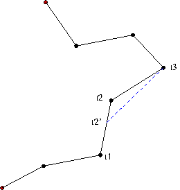
Figure 9.2: Backtracking-based Similar Path Evolution

If the current path is found to be compliant to the coverage hole storage constraint, then it must be checked for the other two constraints as per the priority order. Since the action to be taken if at any node, either of the remaining two constraint fails, is same, we explain testing for these constraints in a common way in the following. Instead of going back all the way back to the start node, we can do a local check in the vicinity of the the intermediate node and find any similar path that may satisfy all the constraints. To find such a similar path, the path in the current iteration is backtracked to one of the “last neighbors” of the node at which the constraint failed (referred as t2), one step at a time. From that neighbor, it is checked if a path can be evolved to the successor of the node at which constraint failed (referred as t3). If we cannot find a neighbor and rescind till the parent of t2 (referred as t1),then we simply forget about t3, block all the nodes on the path segment between t2 and t1, and proceed normally to find alternative path. If the algorithm is able to find some intermediate node that satisfies all the other constraints (minimum route length, maximum angle and line of sight ), we add a path segment between this intermediate node and t3, and allow the testing of this modified path to proceed from node t3 onwards. The entire next iteration is depicted in Figure 9.2.

Blocking of Path Segments

Since we use Theta* as the kernel of brute force algorithm, we also need to take care of other ways via which the path evolved in current iteration relapses and coincides with the path evolved and discarded in the previous iteration. To understand that, one must have a look at Fig. 9.3 and 9.4.

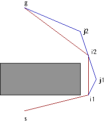
Figure 9.3: Prohibited Brute Force Path Evolution: Case 1

As the brute force path planning for the current iteration evolves from e.g. node $i_{1}$ in the Theta* way, it is possible that ends up coinciding with the previous iterations’ path. If that happens, that implies that in both paths, all segments, including the segment $i_{1}-i_{2}$ are common and overlaid. Since the neighbor of $i_{1}$ was blocked before the current iteration started, this perfect overlay is only possible when line-of-sight based merging happens. That is, the path of current iteration progresses via $i_{1}-j_{2}$ and $j_{2}-i_{2}$ segments, which in turn get triangulated and shorted in lack of any obstacle along segment $i_{1}-i_{2}$. Lack of obstacle is implied since otherwise, that segment could not have been part of the path evolved in previous iteration. To avoid such triangulation to happen, one must not only block the immediate neighbor of $i_{1}$ in previous iteration, but also the immediate segment: $i_{1}-i_{2}$ as well. In such case, during any future iterations beyond the previous iterations, such segments cannot be exactly overlaid on any new path. With respect to Fig. 9.3, this means that the red-colored segment should be blocked out as well, at the end of previous iteration. The path is then forced to evolve and complete as shown in blue color in the same illustration. It is possible for such blocked red segment to be a proper subset of a longer blue segment however, because in that case, the enumeration of paths of both iterations, as successive turning points, will not exactly coincide.

The path coincidence in presence of a coverage hole can be avoided much in the same way. With respect to Fig. 9.4, assume that in the previous iteration, the red-colored path violated the storage constraint related upper threshold. This in turn implies that the path segment of the red path within the coverage hole must not be retraced in the next iteration’s path evolution. Let us assume a convention to represent such a path segment by the node from which the path evolution in the previous iteration entered into the specific coverage hole. Hence, in the current iteration, the path will start evolving from node $e_{1}$, after one blocks out the neighbor of $e_{1}$ as found in the previous iteration. To follow the same blocking mechanism, not only we block the above-mentioned neighboring node of $e_{1}$, we also block the path segment $e_{1}-i_{1}$, belonging to the path of the previous iteration. This will ensure that Theta* does not lead to any triangulation of the kind $e_{1}-j_{1}$ and $j_{1}-i_{1}$ in the current iteration, thus progressing in the same way/path as in the previous iteration. Instead, on blocking such (red-colored) segment $e_{1}-i_{1}$, the path evolution in current iteration is forced to proceed as sequence of non-overlapping $e_{1}-j_{1}$, $j_{1}-j_{2}$ and $j_{2}-g$ segments.

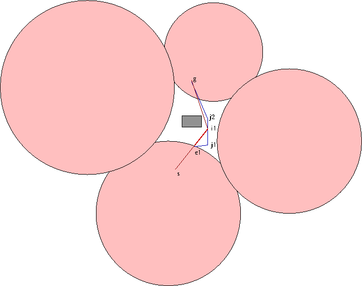
Figure 9.4: Prohibited Brute Force Path Evolution: Case 2

9.3.2 Comparison Results

Comparison of performance of our proposed algorithm was done with brute force algorithm, specifically designed for this purpose as explained earlier. The comparison was done by executing both algorithm for a fixed, same suite of test cases, and observing the set of their execution time for the suite. The test cases were designed so as to represent different type of terrains and obstacles. Backtracking is inherent in both the algorithms and is not deemed to be representing another separate iteration. We further assume that the per-iteration time taken by both algorithms is similar and comparable, since the distance between goal and source node is same for both, and the backtracking strategy is similar. In such a case, it is easy to observe that at a coarse level of measurement, our algorithm takes just 1 iteration, while the brute force testing algorithm was found to take almost 9-10 iterations even for simple test cases. For the test cases having at least 2 coverage holes without any obstacles, the brute-force algorithm was found to take nearly 50 iterations. One must note that the coverage holes which we simulated were very small (approximately 30 cell size each), in comparison to the size of holes that are expected to occur during real deployment.

Generalizing the above observations, it can further be proven that whenever the size of the holes is large,the no. of iterations will increase significantly. The intuition behind the proof is as follows. Figure 9.5 shows the series of paths that are evolved over iterations by the brute force algorithm. In that figure, only some intermediate paths are drawn for better representation. The dotted black lines represent the paths evolved in initial iterations that are not satisfying the coverage hole constrain. The green, non-dotted line is the path obtained after satisfying the coverage hole constraint, since our brute force algorithm is not fully dumb but evolves alternative paths by making the current path compliant to constraints in a priority order, over successive iterations. For this line, while top priority constraint is satisfied, the other constraints are found to fail. Hence in the vicinity of the intermediate node, brute force algorithm will search for some node that can satisfy other constraints. Final correct path is eventually evolved, and is shown in blue color. Given the grid size and the no. of permutations involved in taking short detour via neighbors at non-compliant intermediate nodes, it is imperative if the grid size is large, such sequence of path evolution will take many more iterations to converge. Iterations will be much more when the no. of coverage holes and the obstacles increase beyond what was the maximum number we were able to test with. If we were to compare our algorithm with a pure brute force algorithm, in which random paths are generated between the source and the goal nodes, tested for compliance of constraints, and having no correlation between the path as a sequence of segments between two successive iterations, then it is again imperative that the no. of iterations taken will be even higher. Hence the time performance of our algorithm is better than a brute force baseline algorithm in order of tens.

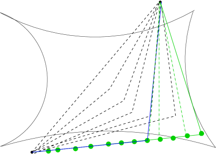
Figure 9.5: Depiction of Iterative Brute Force Evolution of Conformant Path

9.4 Functional Testing

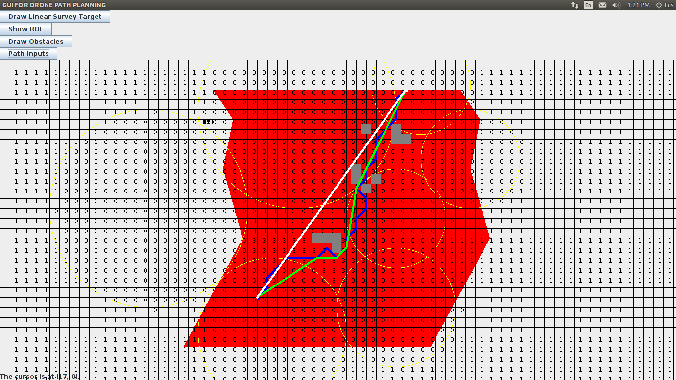
Figure 9.6: Illustration 1 of Functional Test Case

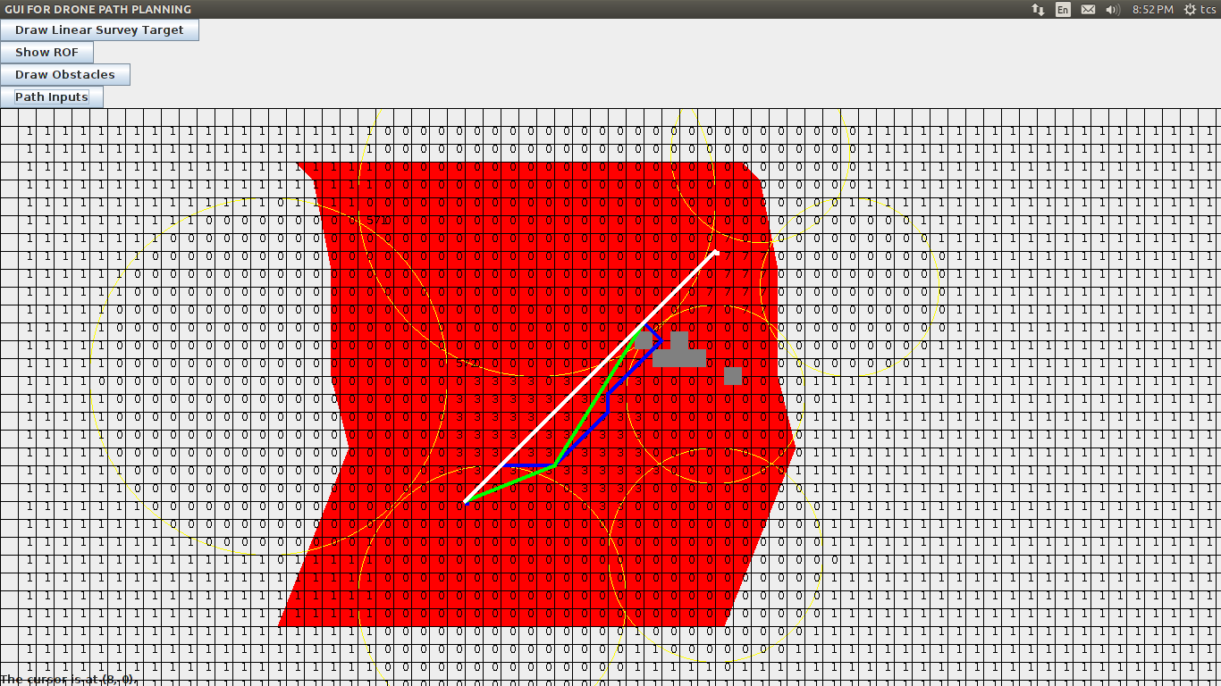
Figure 9.7: Illustration 2 of Functional Test Case

9.5 Simulation Environment

To be able to evaluate, we had to design a more comprehensive simulation environment. This simulation environment is written in Java as a single-threaded application. The simulation environment encompasses a regular grid-based planning environment. It is designed to allow placement of obstacles of any shape and size, as well as coverage holes if needed, at any location. Further, they can be placed at any relative geometric configuration and proximities with respect to one-another. Such freedom entails the obstacles to be placed partially overlapping, fully ensconced within or fully outside one or more coverage holes. The simulation environment further allows specification of source and goal nodes at arbitrary locations, including being within a hole or outside a hole.

9.6 Simulation Results

The additionally evaluated scenarios included permutations of all of the above-mentioned degrees of freedom. Though not exhaustive (around 47 testcases), it did help us in locating many corner cases and checking our algorithm’s readiness to handle those cases. Illustrative evolution of such paths are depicted in Figs. 9.6 and 9.7. We describe the evolution with respect to the firs t figure now. In this figure, partial yellow circles depict the coverage regions, while coverage holes are those regions which aren’t part of any circle. The grey rectangles depict obstacles in various configurations. The red region depicts the flight planning corridor for a infrastructure that hypothetically runs along either the right or the left boundary of the region. The white path depicts the continuous shortest path, the green path depicts the shortest path evolved by our algorithm, and the blue path depicts the sequence of nodes that were visited, neighbor after neighbor, to evolve the final, green path. In the bigger scheme of things, the white line/direct shortest path is not feasible, since remaining constraints (discussed earlier in section 4.5), including the storage constraint modeling the coverage requirement, have to be satisfied as well. Many more complex test scenarios were covered other than the illustrative example here. The broader and structured list of testcases is available on request.

Chapter 10 Conclusion

In the research work so far, we have designed for the maximum communication scenario while aerial path planning. To the best of our knowledge, such scenario, though useful, has not been covered in aerial path planning literature. We have also designed a deterministic backtracking algorithm for angle constraint in presence of obstacles, and in case of storage overflow in coverage holes. A design for scaling the solution for 3D path planning has been devised. One useful thing that we learnt was that the conversion between a scalar cost and the same being enforced as a thresholded constraint is sometimes just a theoretical beauty.

Implementing Storage cost as constraint has made our algorithm too complex, with too many corner cases. While it works, there is always the possibility that another corner case is recognized up all of sudden on a future date, and algorithm may need patching up. Hence a fresh approach for direct biobjective path planning has also been designed.

In future, we are also planning to test our algorithm on Tiger Dataset of 2009. It is a Shortest Path Challenge dataset based on road networks, provided by NSF(nodes of order of $10^{5}$ and beyond). This dataset has to be augmented to contain coverage hole and no-fly zone information, before we can use it as useful input to our algorithm.

References

- [1] Kenny Daniel, Alex Nash, and Sven Koenig. Theta*: Any-angle path planning on grids. Journal of Artificial Intelligence Research, 39:533–579, 2010.
- [2] Yan Li, Hai Chen, Meng Joo Er, and Xinmin Wang. Coverage path planning for {UAVs} based on enhanced exact cellular decomposition method. Elsevier Journal on Mechatronics, 21(5):876–885, 2011.
- [3] H. Sharma and P. Balamuralidhar. A Communication Approach for Aerial Surveillance of Long Linear Infrastructures in Non-urban Terrain. In Twenty First National Conference on Communications, pages 1–6, 2015.
- [4] QinetiQ Group PLC. QinetiQ files for three world records for its Zephyr Solar powered UAV. http://www.qinetiq.com/media/news/releases/Pages/three-world-records.aspx, August 2010. Press Release.
- [5] S.A. Bortoff. Path planning for UAVs. In Proceedings of the 2000 American Control Conference, pages 364–368, 2000.
- [6] Alireza Ghaffarkhah and Yasamin Mostofi. Dynamic networked coverage of time-varying environments in the presence of fading communication channels. ACM Transactions on Sensor Networks, 10(3):45:1–45:38, 2014.
- [7] Chad Goerzen, Zhaodan Kong, and Bernard Mettler. A Survey of Motion Planning Algorithms from the Perspective of Autonomous UAV Guidance. In 2nd International Symposium on UAVs, pages 65–100, 2009.
- [8] Victor Roman. Turn Constrained Path Planning Problems. Master’s thesis, University of Nevada at Las Vegas, 2006.
- [9] Ali Boroujerdi and Jeffrey Uhlmann. An efficient algorithm for computing least cost paths with turn constraints. Information Processing Letters, 67(6):317–321, 1998.
- [10] L. Techy, C.A. Woolsey, and K.A. Morgansen. Planar path planning for flight vehicles in wind with turn rate and acceleration bounds. In IEEE International Conference on Robotics and Automation, pages 3240–3245, 2010.
- [11] Konstantin Yakovlev, Egor Baskin, and Ivan Hramoin. Grid-Based Angle-Constrained Path Planning. In KI 2015: Advances in Artificial Intelligence, volume 9324 of Lecture Notes in Computer Science, pages 208–221. Springer Verlag, 2015.
- [12] Jimmy Krozel, Changkil Lee, and Joseph S B Mitchell. Turn-constrained route planning for avoiding hazardous weather. ATCAI Air Traffic Control Quarterly, 14(2):159–182, 2006.
- [13] Jose Alfredo Guerrero and Yasmina Bestaoui. UAV path planning for structure inspection in windy environments. Journal of Intelligent & Robotic Systems, 69(1-4):297–311, 2013.
- [14] Hu Xu, Lei Shu, and May Huang. Planning Paths with Fewer Turns on Grid Maps. In AAAI International Symposium on Combinatorial Search, pages 193–201, 2013.
- [15] A. Ghaffarkhah and Y. Mostofi. Communication-aware Surveillance in Mobile Sensor Networks. In IEEE American Control Conference, pages 4032–4038, 2011.
- [16] A. Ghaffarkhah and Y. Mostofi. Communication-aware motion planning in mobile networks. Automatic Control, IEEE Transactions on, 56(10):2478–2485, 2011.
- [17] Jerome Le Ny, A. Ribeiro, and G.J. Pappas. Adaptive communication-constrained deployment of unmanned vehicle systems. Selected Areas in Communications, IEEE Journal on, 30(5):923–934, 2012.
- [18] Y. Kantaros and M.M. Zavlanos. Communication-aware Coverage Control for Robotic Sensor Networks. In IEEE Annual Conference on Decision and Control, pages 6863–6868, 2014.
- [19] Y. Mostofi. Communication-aware Motion Planning in Fading Environments. In IEEE International Conference on Robotics and Automation, pages 3169–3174, May 2008.
- [20] A. Ghaffarkhah and Y. Mostofi. Communication-aware Navigation Functions for Cooperative Target Tracking. In IEEE American Control Conference, pages 1316–1322, June 2009.
- [21] A. Ghaffarkhah and Y. Mostofi. Channel learning and Communication-aware Motion Planning in Mobile Networks. In IEEE American Control Conference, pages 5413–5420, 2010.
- [22] Y. Mostofi, M. Malmirchegini, and A. Ghaffarkhah. Estimation of Communication Signal Strength in Robotic Networks. In IEEE International Conference on Robotics and Automation, pages 1946–1951, 2010.
- [23] Magnus Lindhe. Communication-Aware Motion Planning for Mobile Robots. PhD thesis, KTH Royal Institute of Technology, 2012.
- [24] Yasamin Mostofi. Decentralized communication-aware motion planning in mobile networks: An information-gain approach. Springer Journal of Intelligent and Robotic Systems, 56(2):233–256, 2009.
- [25] Yi-Ge Fu, Jie Zhou, and Lei Deng. Surveillance of a 2d plane area with 3d deployed cameras. MDPI Journal of Sensors, 14(2):1988–2011, 2014.
- [26] Baro Hyun, Pierre Kabamba, and Anouck Girard. Optimally-informative path planning for dynamic bayesian classification. Springer Optimization Letters, 6(8):1627–1642, 2012.
- [27] Yuan Yan and Y. Mostofi. Efficient communication-aware Dynamic Coverage using Space-filling Curves. In IEEE American Control Conference, pages 964–971, 2014.
- [28] A. Ghaffarkhah and Y. Mostofi. Communication-aware Target Tracking using Navigation Functions - Centralized case. In International Conference on Robot Communication and Coordination, pages 1–8, 2009.
- [29] Kaarthik Sundar. Motion Planning for Unmanned Aerial Vehicles with Resource Constraints. Master’s thesis, Texas A&M University, 2012.
- [30] A. Ghaffarkhah and Y. Mostofi. Path planning for networked robotic surveillance. IEEE Transactions on Signal Processing, 60(7):3560–3575, 2012.
- [31] Dasol Lee and David Hyunchul Shim. Path Planner based on Bidirectional Spline-RRT* for Fixed-wing UAVs. In International Conference on Unmanned Aircraft Systems, pages 77–86, 2016.
- [32] Myung Hwangbo, James Kuffner, and Takeo Kanade. Efficient Two-phase 3D Motion Planning for Small Fixed-wing UAVs. In IEEE International Conference on Robotics and Automation, pages 1035–1041, 2007.
- [33] Parikshit Maini and PB Sujit. Path Planning for a UAV with Kinematic Constraints in the Presence of Polygonal Obstacles. In International Conference on Unmanned Aircraft Systems, pages 62–67, 2016.
- [34] John Canny and John Reif. New Lower bound Techniques for Robot Motion Planning Problems. In IEEE Annual Symposium on Foundations of Computer Science, pages 49–60, 1987.
- [35] Johannes O. Royset, W. Matthew Carlyle, and R. Kevin Wood. Routing Military Aircraft with a Constrained Shortest-path Algorithm. Public report, Naval Postgraduate School, 2007.
- [36] R.J. Szczerba, P. Galkowski, I.S. Glicktein, and N. Ternullo. Robust algorithm for real-time route planning. IEEE Transactions on Aerospace and Electronic Systems, 36(3):869–878, 2000.
- [37] Luca De Filippis, Giorgio Guglieri, and Fulvia Quagliotti. Path planning strategies for uavs in 3d environments. Springer Journal of Intelligent & Robotic Systems, 65(4):247–264, 2012.
- [38] Alex Nash, Sven Koenig, and Craig Tovey. Lazy Theta*: Any-Angle Path Planning and Path Length Analysis in 3D. In AAAI International Conference on Artificial Intelligence, pages 147–154, 2010.
- [39] Ting-Yun Chi, Yi Ming, Tseng, Sy-Yen Kuo, and Chih-Chiun Liao. Civil UAV Path Planning Algorithm for Considering Connection with Cellular Data Network. In International Conference on Computer and Information Technology, pages 327–331, 2012.
- [40] Luitpold Babel. Three-dimensional route planning for unmanned aerial vehicles in a risk environment. Journal of Intelligent & Robotic Systems, 71(2):255–269, 2013.
- [41] Jorge Nocedal and Stephen J. Wright. Numerical Optimization. Springer Science+Business Media Ltd., 2006.
- [42] Hugh Osborne and Lukáš Chrpa. Towards a trajectory planning concept: Augmenting path planning methods by considering speed limit constraints. Journal of Intelligent & Robotic Systems, 75:243–270, 2014.
- [43] Peter Gregory and Lukáš Chrpa. Abstract Augmented Lazy Theta*: Applying Graph Abstractions to Trajectory Planning with Speed-Limit Constraints. In 31st Workshop of the UK Planning & Scheduling Special Interest Group, pages 15–23, 2014.
- [44] Luca De Filippis and Giorgio Guglieri. Advanced Graph Search Algorithms for Path Planning of Flight Vehicles. In Recent Advances in Aircraft Technology, pages 157–193. Intech Open, 2012.
- [45] Petrisor Parvu and Alexandru Parvu. Dynamic Star Search Algorithms for Path Planning of Flight Vehicles. In International Workshop on Numerical Modeling in Aerospace Sciences, pages 193–201, 2013.
- [46] Zhang Qi, Zhenhai Shao, Yeo Swee Ping, Lim Meng Hiot, and Yew Kong Leong. An improved heuristic algorithm for uav path planning in 3d environment. In International Conference on Intelligent Human-Machine Systems and Cybernetics, volume 2, pages 258–261, 2010.
- [47] Bo bo Meng and Xiaoguang Gao. UAV Path Planning Based on Bidirectional Sparse A* Search Algorithm. In International Conference on Intelligent Computation Technology and Automation, pages 1106–1109, 2010.
- [48] Zhi-hong Peng, Jin-ping Wu, and Jie Chen. Three-dimensional multi-constraint route planning of unmanned aerial vehicle low-altitude penetration based on coevolutionary multi-agent genetic algorithm. Journal of Central South University of Technology, 18(5):1502–1508, 2011.
- [49] Hrishikesh Sharma, Tanima Dutta, Adithya V., and Balamuralidhar P. A Real-time Framework for Detection of Long Linear Infrastructural Objects in Aerial Imagery. In International Conference on Image Analysis and Recognition, Lecture Notes in Computer Science. Springer Verlag, 2015.
- [50] Hrishikesh Sharma, Adithya V., Tanima Dutta, and Balamuralidhar P. Image Analysis-based Automatic Utility Pole Detection for Remote Surveillance. In IEEE International Conference on Image Analysis and Recognition, 2015.
- [51] Daniel Delling, Peter Sanders, Dominik Schultes, and Dorothea Wagner. Engineering Route Planning Algorithms. In Algorithmics of Large and Complex Networks, volume 5515 of Lecture Notes in Computer Science, pages 117–139. Springer Berlin Heidelberg, 2009.
- [52] A. Nash, S. Koenig, and M. Likhachev. Incremental Phi*: Incremental Any-Angle Path Planning on Grids. In International Joint Conference on Artificial Intelligence, pages 1824–1830, 2009.
- [53] Jongrae Kim and João P. Hespanha. Discrete Approximations to Continuous Shortest-Path: Application to Minimum-Risk Path Planning for Groups of UAVs. In IEEE International Conference on Decision and Control, 2003.
- [54] M. Garcia, A. Viguria, and A. Ollero. Dynamic graph-search algorithm for global path planning in presence of hazardous weather. Springer Journal of Intelligent & Robotic Systems, 69(4):285–295, 2013.
- [55] Hanguen Kim, Donghoon Kim, Jae-Uk Shin, Hyongjin Kim, and Hyun Myung. Angular rate-constrained path planning algorithm for unmanned surface vehicles. Elsevier Journal of Ocean Engineering, 84:37–44, 2014.
- [56] O. Arslan, P. Tsiotras, and X. Huo. Solving Shortest Path Problems with Curvature Constraints using Beamlets. In IEEE/RSJ International Conference on Intelligent Robots and Systems, pages 3533–3538, 2011.
- [57] Fajie Li and Reinhard Klette. Euclidean Shortest Paths. Springer Verlag, 2011.
- [58] T. Uras and S. Koenig. An Empirical Comparison of Any-Angle Path-Planning Algorithms. In AAAI Symposium on Combinatorial Search, pages 206–211, 2015.
- [59] Heuristics: Amit’s Notes on Pathfinding. http://theory.stanford.edu/~amitp/GameProgramming/Heuristics.html, 1997.
- [60] Sanjiv Kapoor, SN Maheshwari, and Joseph SB Mitchell. An efficient algorithm for euclidean shortest paths among polygonal obstacles in the plane. Discrete & Computational Geometry, 18(4):377–383, 1997.
- [61] John Hershberger and Subhash Suri. An optimal algorithm for euclidean shortest paths in the plane. SIAM Journal on Computing, 28(6):2215–2256, 1999.
- [62] Lyudmil Aleksandrov, Anil Maheshwari, and J-R Sack. Determining approximate shortest paths on weighted polyhedral surfaces. Journal of the ACM (JACM), 52(1):25–53, 2005.
- [63] Frank Neumann, Dirk Sudholt, and Carsten Witt. Computational Complexity of Ant Colony Optimization and Its Hybridization, chapter 10. Springer, 2009.