Layout of random circulant graphs

Sebastian Richter Fakultät für Mathematik, Technische Universität Chemnitz, D-09107 Chemnitz, Germany. sebastian.richter@mathematik.tu-chemnitz.de  and  Israel Rocha The Czech Academy of Sciences, Institute of Computer Science, Pod Vodárenskou věží 2, 182 07 Prague, Czech Republic. With institutional support RVO:67985807. rocha@cs.cas.cz
Abstract.

A circulant graph H𝐻H is defined on the set of vertices V={1,,n}𝑉1𝑛V=\left\{1,\ldots,n\right\} and edges E={(i,j):|ij|s(modn),sS},𝐸conditional-set𝑖𝑗formulae-sequence𝑖𝑗𝑠mod𝑛𝑠𝑆E=\left\{\left(i,j\right):\left|i-j\right|\equiv s\left(\textrm{mod}n\right),s\in S\right\}, where S{1,,n12}.𝑆1𝑛12S\subseteq\left\{1,\ldots,\lceil\frac{n-1}{2}\rceil\right\}. A random circulant graph results from deleting edges of H𝐻H with probability 1p1𝑝1-p. We provide a polynomial time algorithm that approximates the solution to the minimum linear arrangement problem for random circulant graphs. We then bound the error of the approximation with high probability.

Key words and phrases:
Random graphs; Geometric graphs; Circulant Matrices; Random Matrices; Rank correlation coefficient
2000 Mathematics Subject Classification:
05C50; 05C85; 15A52; 15A18
Richter thanks the Institute of Computer Science of The Czech Academy of Sciences, and the Czech Science Foundation, under the grant number GJ16-07822Y, for travel support.
Rocha was supported by the Czech Science Foundation, grant number GJ16-07822Y

1. Introduction

A layout on the graph G=(V,E)𝐺𝑉𝐸G=(V,E) is a bijection function f:V{1,,|V|}:𝑓𝑉1𝑉f:V\rightarrow\left\{1,\dots,\left|V\right|\right\}. Layout problems can be used to formulate several well-known optimization problems on graphs. Also known as linear ordering problems or linear arrangement problems, they consist on the minimization of specific metrics. Such metrics would provide the solution to problems as linear arrangement, bandwidth, modified cut, cut width, sum cut, vertex separation and edge separation. All these problems are NP-hard in the general case.

The Minimum Linear Arrangement (MinLA) problem is to find a function f𝑓f that minimizes the sum uvE|f(u)f(v)|.subscript𝑢𝑣𝐸𝑓𝑢𝑓𝑣\sum_{uv\in E}\left|f(u)-f(v)\right|. A layout is also called a labeling, a ordering, or a linear arrangement. The MinLA is one of the most important graph layout problems and was introduced in 1964 by Harper to develop error-correcting codes with minimal average absolute errors. In fact, MinLA appear in a vast domain of problems: VLSI circuit design, network reliability, topology awareness of overlay networks, single machine job scheduling, numerical analysis, computational biology, information retrieval, automatic graph drawing, etc. For instance, layout problems appear in the reconstruction of DNA sequences [6], using overlaps of genes between fragments. Also, MinLA has been used in brain cortex modelling [7]. In [5] it is presented a good survey on graph layout problems and its applications.

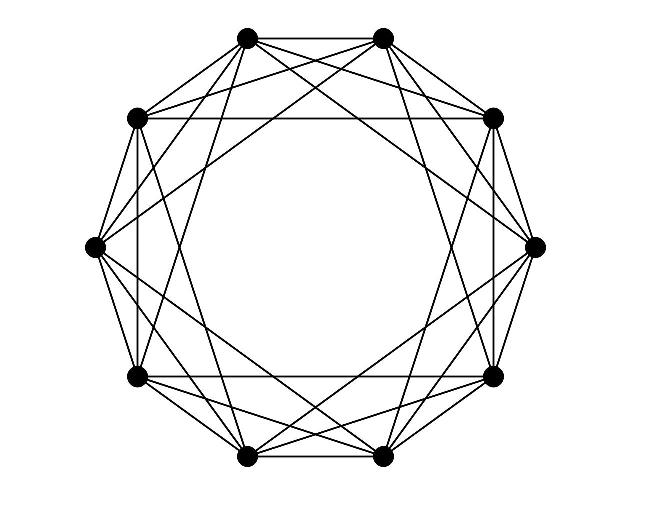
The main contribution of this paper is a polynomial time algorithm that approximates the solution to the MinLA problem for a random circulant graph. First, a circulant graph H𝐻H is defined on the set of vertices V={1,,n}𝑉1𝑛V=\left\{1,\ldots,n\right\} and edges E={(i,j):|ij|s(modn),sS},𝐸conditional-set𝑖𝑗formulae-sequence𝑖𝑗𝑠mod𝑛𝑠𝑆E=\left\{\left(i,j\right):\left|i-j\right|\equiv s\left(\textrm{mod}n\right),s\in S\right\}, where S{1,,n12}.𝑆1𝑛12S\subseteq\left\{1,\ldots,\lceil\frac{n-1}{2}\rceil\right\}. A random circulant graph results from deleting edges of H𝐻H with probability 1p1𝑝1-p. Noticeable, circulant graphs and its random instances carry a nice shape. The MinLA problem for these graphs is the reconstruction of that shape.

Refer to caption
Figure 1.1. Circulant graphs

The MinLA problem for circulant graphs is solved in [8], where the authors address the problem of finding an embedding of G𝐺G into a graph H𝐻H. In that case, G𝐺G is a circulant graph and H𝐻H is a cycle graph. Certain circulant graphs are of particular interest. In [10] it is presented a polynomial time algorithm solving MinLA of Chord graphs, which is a particular case of circulant graphs. The main motivation of [10] is an application to topology awareness of peer-to-peer overlay networks. The solution of [10] assumes that the Chord graph is complete. However, in real overlay networks nodes can disconnect at any moment, so the remaining network can be regarded as a random circulant graph. Thus, the solution to MinLA for random circulant graphs suits well such applications.

Nevertheless, layout problems for random graphs are significantly more complicated and usually the solution is an approximation of the solution of the model graph. The paper [5] is concerned with the approximability of several layout problems on families of random geometric graphs. It is proven that some of these problems are still NP-complete even for deterministic geometric graphs. The authors present heuristics that turn out to be constant approximation algorithms for layout problems on random geometric graphs, almost surely. The authors of [5] remark that their algorithms use the node coordinates in order to build a layout. That is another feature we do not require in our problem. Even tough, the random graph follows a geometric graph model (the circulant structure), we do not have the coordinates of the random graph in advance. The input random graph consists of a set of vertices and edges only and we have to retrieve the circulant layout from that.

Eigenvectors of random matrices are the main tool we use to construct the layout in our problem. We introduce this idea in [9], where one eigenvector would suffice to recover the structure of a random linear graph. Here, as we will see, one eigenvector alone is not enough to encode the whole layout. Fortunately, we can combine two special eigenvectors to find the linear arrangement. Even tough, the use of eigenvectors in the same fashion is a common feature of both methods, here we require some additional technical details that were not present in [9]. Due to the use of angles between subspaces and SVD decomposition, the technique we use here differs significantly from [9]. There, we pointed out the generality of such method and here it turns out we need a more careful analysis. Nevertheless, we have evidence that these methods can be used to implement a general framework for which layout problems can be solved in a broader class of random geometric graphs.

The rest of the paper is organized as follow. In section 2 we define the model matrix, state the algorithm, and the main theorems. In section 3 we describe basic properties of angle between subspaces. Finally, in section 4 we provide the proofs for the results.

2. Main results

A circulant matrix A𝐴A is a matrix that can be completely specified by only one vector a𝑎a, that appears in the first column of A𝐴A. The remaining columns are cyclic permutations of a𝑎a with offset equal to the column index, i.e., the matrix A𝐴A is of the following form

A=[a1a2a3anana1a2an1a2a3a4a1].𝐴matrixsubscript𝑎1subscript𝑎2subscript𝑎3subscript𝑎𝑛subscript𝑎𝑛subscript𝑎1subscript𝑎2subscript𝑎𝑛1missing-subexpressionmissing-subexpressionsubscript𝑎2subscript𝑎3subscript𝑎4subscript𝑎1A=\begin{bmatrix}a_{1}&a_{2}&a_{3}&\dots&a_{n}\\ a_{n}&a_{1}&a_{2}&\dots&a_{n-1}\\ \vdots&&\ddots&&\vdots\\ a_{2}&a_{3}&a_{4}&\dots&a_{1}\end{bmatrix}.

A circulant graph is a graph with circulant adjacency matrix. Let H=(V,EH)𝐻𝑉subscript𝐸𝐻H=(V,E_{H}) be a circulant graph with vertex set V={v1,,vn}𝑉subscript𝑣1subscript𝑣𝑛V=\{v_{1},\dots,v_{n}\} and adjacency matrix A𝐴A, where [a1,,an]subscript𝑎1subscript𝑎𝑛[a_{1},...,a_{n}] corresponds to the first row of A𝐴A. We define the set of indices of non-zero elements in the first half of the row of A𝐴A as

N:={k:ak=1,1kn12}.assign𝑁conditional-set𝑘formulae-sequencesubscript𝑎𝑘11𝑘𝑛12N:=\{k:a_{k}=1,1\leq k\leq\lceil\frac{n-1}{2}\rceil\}.

Equivalently, a circulant graph can be defined as the Cayley graph of a finite cyclic group.

In this paper, H𝐻H is referred as the model graph. The random graph we consider is denoted by G=(V,E)𝐺𝑉𝐸G=(V,E) which results from deleting edges of H𝐻H with probability 1p.1𝑝1-p. The model matrix M𝑀M is a circulant matrix that describes the structure of H𝐻H, where M=pA𝑀𝑝𝐴M=pA.

Refer to caption

M=p[0111000111101110001111011100011110111000011101110000111011100001110111100011101111000111011110001110]𝑀𝑝matrix0111000111101110001111011100011110111000011101110000111011100001110111100011101111000111011110001110M=p\begin{bmatrix}0&{\color[rgb]{0,0,1}1}&{\color[rgb]{0,0,1}1}&{\color[rgb]{0,0,1}1}&0&0&0&{\color[rgb]{0,0,1}1}&{\color[rgb]{0,0,1}1}&{\color[rgb]{0,0,1}1}\\ {\color[rgb]{0,0,1}1}&0&{\color[rgb]{0,0,1}1}&{\color[rgb]{0,0,1}1}&{\color[rgb]{0,0,1}1}&0&0&0&{\color[rgb]{0,0,1}1}&{\color[rgb]{0,0,1}1}\\ {\color[rgb]{0,0,1}1}&{\color[rgb]{0,0,1}1}&0&{\color[rgb]{0,0,1}1}&{\color[rgb]{0,0,1}1}&{\color[rgb]{0,0,1}1}&0&0&0&{\color[rgb]{0,0,1}1}\\ {\color[rgb]{0,0,1}1}&{\color[rgb]{0,0,1}1}&{\color[rgb]{0,0,1}1}&0&{\color[rgb]{0,0,1}1}&{\color[rgb]{0,0,1}1}&{\color[rgb]{0,0,1}1}&0&0&0\\ 0&{\color[rgb]{0,0,1}1}&{\color[rgb]{0,0,1}1}&{\color[rgb]{0,0,1}1}&0&{\color[rgb]{0,0,1}1}&{\color[rgb]{0,0,1}1}&{\color[rgb]{0,0,1}1}&0&0\\ 0&0&{\color[rgb]{0,0,1}1}&{\color[rgb]{0,0,1}1}&{\color[rgb]{0,0,1}1}&0&{\color[rgb]{0,0,1}1}&{\color[rgb]{0,0,1}1}&{\color[rgb]{0,0,1}1}&0\\ 0&0&0&{\color[rgb]{0,0,1}1}&{\color[rgb]{0,0,1}1}&{\color[rgb]{0,0,1}1}&0&{\color[rgb]{0,0,1}1}&{\color[rgb]{0,0,1}1}&{\color[rgb]{0,0,1}1}\\ {\color[rgb]{0,0,1}1}&0&0&0&{\color[rgb]{0,0,1}1}&{\color[rgb]{0,0,1}1}&{\color[rgb]{0,0,1}1}&0&{\color[rgb]{0,0,1}1}&{\color[rgb]{0,0,1}1}\\ {\color[rgb]{0,0,1}1}&{\color[rgb]{0,0,1}1}&0&0&0&{\color[rgb]{0,0,1}1}&{\color[rgb]{0,0,1}1}&{\color[rgb]{0,0,1}1}&0&{\color[rgb]{0,0,1}1}\\ {\color[rgb]{0,0,1}1}&{\color[rgb]{0,0,1}1}&{\color[rgb]{0,0,1}1}&0&0&0&{\color[rgb]{0,0,1}1}&{\color[rgb]{0,0,1}1}&{\color[rgb]{0,0,1}1}&0\end{bmatrix}

Figure 2.1. Model graph and its model matrix

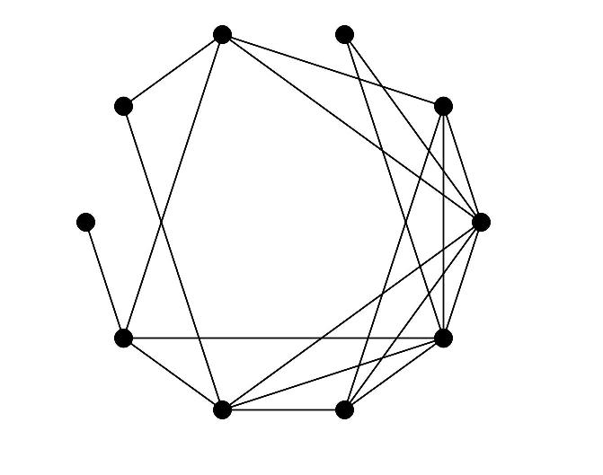
Furthermore, let M^^𝑀\hat{M} be the adjacency matrix of the random graph G𝐺G. The entries of M^^𝑀\hat{M} correspond to independent Bernoulli variables, where 𝐏(m^ij=1)=mij.𝐏subscript^𝑚𝑖𝑗1subscript𝑚𝑖𝑗\mathbf{P}(\hat{m}_{ij}=1)=m_{ij}.
Refer to caption

M^=[0011000101000110000010011100001110111000011101110000111010000001110101100010101000000001001000000100]^𝑀matrix0011000101000110000010011100001110111000011101110000111010000001110101100010101000000001001000000100\hat{M}=\begin{bmatrix}0&0&{\color[rgb]{0,0,1}1}&{\color[rgb]{0,0,1}1}&0&0&0&{\color[rgb]{0,0,1}1}&0&{\color[rgb]{0,0,1}1}\\ 0&0&0&{\color[rgb]{0,0,1}1}&{\color[rgb]{0,0,1}1}&0&0&0&0&0\\ {\color[rgb]{0,0,1}1}&0&0&{\color[rgb]{0,0,1}1}&{\color[rgb]{0,0,1}1}&{\color[rgb]{0,0,1}1}&0&0&0&0\\ {\color[rgb]{0,0,1}1}&{\color[rgb]{0,0,1}1}&{\color[rgb]{0,0,1}1}&0&{\color[rgb]{0,0,1}1}&{\color[rgb]{0,0,1}1}&{\color[rgb]{0,0,1}1}&0&0&0\\ 0&{\color[rgb]{0,0,1}1}&{\color[rgb]{0,0,1}1}&{\color[rgb]{0,0,1}1}&0&{\color[rgb]{0,0,1}1}&{\color[rgb]{0,0,1}1}&{\color[rgb]{0,0,1}1}&0&0\\ 0&0&{\color[rgb]{0,0,1}1}&{\color[rgb]{0,0,1}{\color[rgb]{0,0,1}1}}&{\color[rgb]{0,0,1}1}&0&{\color[rgb]{0,0,1}1}&0&0&0\\ 0&0&0&{\color[rgb]{0,0,1}1}&{\color[rgb]{0,0,1}1}&{\color[rgb]{0,0,1}1}&0&{\color[rgb]{0,0,1}1}&0&{\color[rgb]{0,0,1}1}\\ {\color[rgb]{0,0,1}1}&0&0&0&{\color[rgb]{0,0,1}1}&0&{\color[rgb]{0,0,1}1}&0&{\color[rgb]{0,0,1}1}&0\\ 0&0&0&0&0&0&0&{\color[rgb]{0,0,1}1}&0&0\\ {\color[rgb]{0,0,1}1}&0&0&0&0&0&0&{\color[rgb]{0,0,1}1}&0&0\end{bmatrix}

Figure 2.2. Random graph and its random matrix

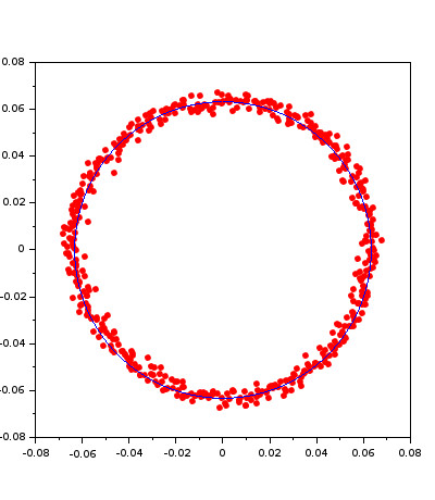
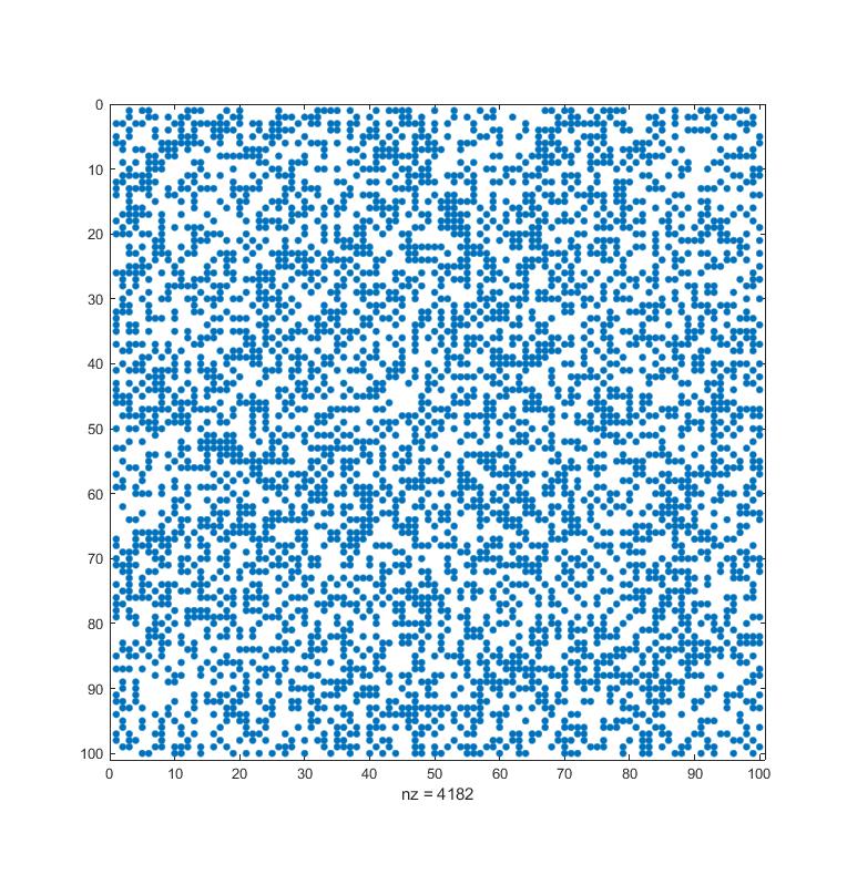
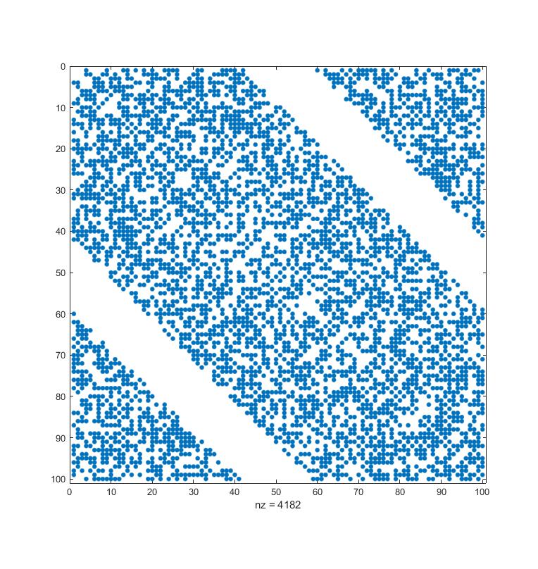
By construction, the labels of vertices in the random graph G𝐺G corresponds to the same labels as the graph model in the first figure. However, in the real world we do not have the labels in advance. We are talking about a large amount of disorganized data with additional noise. We only know that this data encodes a circulant structure which is hidden from us. In such situations, finding the labels for the random graph can be rather challenging. See Figure 2.3.
Refer to caption
Refer to caption
Figure 2.3. Data before and after the correct permutation.

That is precisely the problem we address in this paper: given a graph that follows a circulant model, find its circular embedding, or rather, retrieve the correct order of the vertices. We present an algorithm that solves this problem by using eigenvectors corresponding the second and third largest eigenvalues M^^𝑀\hat{M}. The algorithm can be described as follow.

1:Random matrix M^^𝑀\widehat{M}
2:Compute x^^𝑥\widehat{x} and y^^𝑦\widehat{y}, the eigenvectors for λ2(M^)subscript𝜆2^𝑀\lambda_{2}(\widehat{M}) and λ3(M^)subscript𝜆3^𝑀\lambda_{3}(\widehat{M})
3:Compute the angular coordinate φisubscript𝜑𝑖\varphi_{i} for the point of coordinates (xi^,yi^)^subscript𝑥𝑖^subscript𝑦𝑖(\widehat{x_{i}},\widehat{y_{i}})
4:Define a permutation σ𝜎\sigma such that σ(i)>σ(j)𝜎𝑖𝜎𝑗\sigma(i)>\sigma(j) iff φiφjsubscript𝜑𝑖subscript𝜑𝑗\varphi_{i}\geq\varphi_{j}
5:return σ𝜎\sigma
Algorithm 1

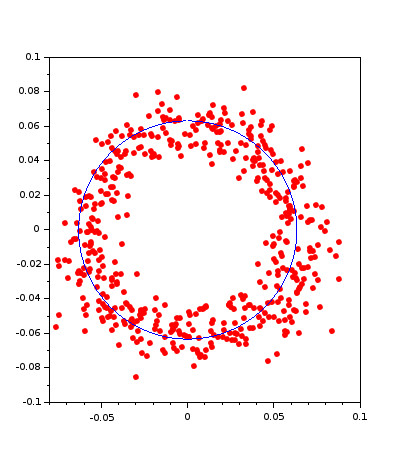
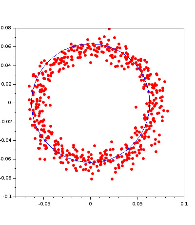
This simple algorithm is shown to return the correct labels with a bounded error. We quantify the error in terms of a rank correlation coefficient we introduce. Before, let us plot the points described in Algorithm 1.
Refer to caption
Refer to caption
Refer to caption
Figure 2.4. Points whose coordinates are entries of the eigenvectors. Probabilities: 0.3, 0.5, 0.9.

The circle-like shape follows indeed the layout we are looking to reconstruct. This phenomenon can be explained in terms of angles between spaces which appear in our proofs. Also, notice that the points that are in the wrong position are not a major part. That can be explained in terms of rank correlation coefficients.

A rank correlation coefficient measures the degree of similarity between two lists, and can be used to assess the significance of the relation between them. One can see the rank of one list as a permutation of the rank of the other. Statisticians have used a number of different measures of closeness for permutations. Some popular rank correlation statistics are Kendall’s τ𝜏\tau, Kendall distance, and Spearman’s footrule. There are several other metrics, and for different situations some metrics are preferable. For a deeper discussion on metrics on permutations we recommend [4].

To count the total number of inversions in σ𝜎\sigma one can use

D(σ)=i<j1σ(i)>σ(j) (Kendall Distance)𝐷𝜎subscript𝑖𝑗subscript1𝜎𝑖𝜎𝑗 (Kendall Distance)D(\sigma)=\sum_{i<j}\textbf{1}_{\sigma(i)>\sigma(j)}\text{ (Kendall Distance)}

First we define a refined version of the Kendall distance. This version counts inverted pairs whose indices are at least k𝑘k positions apart. First note that, for a permutation σ𝜎\sigma, we can rewrite D(σ)𝐷𝜎D(\sigma) as

D(σ)=|{(i,j):σ(j)<σ(i) and i<j}|.𝐷𝜎conditional-set𝑖𝑗𝜎𝑗𝜎𝑖 and 𝑖𝑗D(\sigma)=|\{(i,j):\sigma(j)<\sigma(i)\mbox{ and }i<j\}|.

Given a permutation σ𝜎\sigma and an index k1𝑘1k\geq 1, let

Dk(σ)=|{(i,j):σ(j)<σ(i) and i+kjand ijkmodn}|.subscript𝐷𝑘𝜎conditional-set𝑖𝑗𝜎𝑗𝜎𝑖 and 𝑖𝑘𝑗and 𝑖𝑗𝑘mod𝑛D_{k}(\sigma)=|\{(i,j):\sigma(j)<\sigma(i)\textrm{ and }i+k\leq j\ \text{and }i-j\geq k\ \textrm{mod}\ n\}|.

Thus, Dksubscript𝐷𝑘D_{k} counts the number of inverted pairs where the vertices have jumped at least k𝑘k positions from their original order. In particular, D1(σ)=D(σ)subscript𝐷1𝜎𝐷𝜎D_{1}(\sigma)=D(\sigma). The module in the definition is used to access the circular structure of the graph we consider.

Consider the eigenvectors x𝑥x and y𝑦y for λ2(M)subscript𝜆2𝑀\lambda_{2}(M) and λ3(M)subscript𝜆3𝑀\lambda_{3}(M), respectively. As we will see, the set of points zi=(xi,yi)subscript𝑧𝑖subscript𝑥𝑖subscript𝑦𝑖z_{i}=(x_{i},y_{i}) have coordinates on a circle in 2superscript2\mathbb{R}^{2}. Let φ(x)𝜑𝑥\varphi(x) be the angular coordinate for x2𝑥superscript2x\in\mathbb{R}^{2}. A crucial observation is that {φ(zi)}i=1nsuperscriptsubscript𝜑subscript𝑧𝑖𝑖1𝑛\left\{\varphi(z_{i})\right\}_{i=1}^{n} is an increasing sequence. That means that the order of φ(zi)𝜑subscript𝑧𝑖\varphi(z_{i}) provides the correct order for the vertices in the model graph. Similarly, we can consider the eigenvectors x^^𝑥\widehat{x} and y^^𝑦\widehat{y} for λ2(M^)subscript𝜆2^𝑀\lambda_{2}(\widehat{M}) and λ3(M^)subscript𝜆3^𝑀\lambda_{3}(\widehat{M}), respectively. Here, {φ(zi^)}i=1nsuperscriptsubscript𝜑^subscript𝑧𝑖𝑖1𝑛\left\{\varphi(\widehat{z_{i}})\right\}_{i=1}^{n} does not necessarily form an increasing sequence. Thus, we can construct a permutation σ𝜎\sigma of indices such that σ(i)>σ(j)𝜎𝑖𝜎𝑗\sigma(i)>\sigma(j) if and only if φ(zi^)φ(zj^)𝜑^subscript𝑧𝑖𝜑^subscript𝑧𝑗\varphi(\widehat{z_{i}})\geq\varphi(\widehat{z_{j}}).

In view of the last observations, the permutation σ𝜎\sigma has a neat interpretation in terms of Dksubscript𝐷𝑘D_{k}: Dk(σ)subscript𝐷𝑘𝜎D_{k}(\sigma) counts the pairs in z^^𝑧\hat{z} that disagree with the order induced by z𝑧z by at least k𝑘k positions. I.e, the permutation σ𝜎\sigma of Algorithm 1 has Dk(σ)subscript𝐷𝑘𝜎D_{k}(\sigma) pairs of vertices in the wrong order. Fortunately, the next Theorem bounds the number of such pairs.

Theorem 1.

Let σ𝜎\sigma be the permutation returned by Algorithm 1 for a random circulant graph. Let kΩ(nβ)𝑘Ωsuperscript𝑛𝛽k\in\Omega(n^{\beta}) and |N|=cn𝑁𝑐𝑛|N|=cn, for a constant c>0𝑐0c>0. Then it holds Dk(σ)𝒪(n54β)subscript𝐷𝑘𝜎𝒪superscript𝑛54𝛽D_{k}(\sigma)\in\mathcal{O}(n^{5-4\beta}) with probability 1n31superscript𝑛31-n^{-3}.

In fact, we prove a more general version of Theorem 1 where we allow the edge density to be variable.

Theorem 2.

Let σ𝜎\sigma be the permutation returned by Algorithm 1 for a random circulant graph with model satisfying |N|=cnγ𝑁𝑐superscript𝑛𝛾|N|=cn^{\gamma}, for a constant c>0𝑐0c>0. Let kΩ(nβ).𝑘Ωsuperscript𝑛𝛽k\in\Omega(n^{\beta}). Then we have Dk(σ)𝒪(n116γ4β)subscript𝐷𝑘𝜎𝒪superscript𝑛116𝛾4𝛽D_{k}(\sigma)\in\mathcal{O}(n^{11-6\gamma-4\beta}) with probability 1n31superscript𝑛31-n^{-3}.

Furthermore, depending on the parameters γ𝛾\gamma and β𝛽\beta we can improve the bounds of the last Theorems, as shown in the next result.

Theorem 3.

Let σ𝜎\sigma be the permutation returned by Algorithm 1 for a random circulant graph with model satisfying |N|=cnγ𝑁𝑐superscript𝑛𝛾|N|=cn^{\gamma}, for a constant c>0𝑐0c>0. Let kΩ(nβ).𝑘Ωsuperscript𝑛𝛽k\in\Omega(n^{\beta}). Then we have Dk(σ)𝒪(n136γ2β3)subscript𝐷𝑘𝜎𝒪superscript𝑛136𝛾2𝛽3D_{k}(\sigma)\in\mathcal{O}(n^{\frac{13-6\gamma-2\beta}{3}}) with probability 1n31superscript𝑛31-n^{-3}.

Notice that the last result shows that there is a trade off between how far vertices can jump and the total number of such incorrectly placed vertices. That is useful for our purpose to establish metrics on the correctness of the rank. For example, consider the worst case of Theorem 3 when all pairs are incorrect. Assuming γ=1𝛾1\gamma=1, the number of pairs that drift less than k𝑘k positions apart is (n2)Dkbinomial𝑛2subscript𝐷𝑘\binom{n}{2}-D_{k}. If we take β>1/2𝛽12\beta>1/2 in Theorem 3 , we obtain that (n2)Dkbinomial𝑛2subscript𝐷𝑘\binom{n}{2}-D_{k} is asymptotically equivalent to n2superscript𝑛2n^{2} as n𝑛n\rightarrow\infty. That means almost no vertex will drift more than n1/2superscript𝑛12n^{1/2} slots from its correct position.

Finally, the next theorem shows that the permutation returned by Algorithm 1 is well behaved in terms of the usual Kendall distance.

Theorem 4.

Let σ𝜎\sigma be the permutation returned by Algorithm 1 for a random circulant graph with model satisfying |N|=cnγ𝑁𝑐superscript𝑛𝛾|N|=cn^{\gamma} and 1γ>01𝛾01\geq\gamma>0. Then D(σ)𝒪(n(156γ)/5)𝐷𝜎𝒪superscript𝑛156𝛾5D(\sigma)\in\mathcal{O}(n^{(15-6\gamma)/5}) with probability 1n31superscript𝑛31-n^{-3}.

To prove the results, our technique uses Singular Value Decomposition and angles between subspaces, which require expressions for the eigenvalues and eigenvectors of the model matrix. Fortunately, circulant matrices have known spectrum and, as we will see, there is a specific pair of eigenvectors carrying the desired information about the structure of the graph, providing the correct label of vertices. Moreover, consecutive entries of the eigenvectors differ significantly enough so that a small perturbation will have limited effect on the labels. Further, in Section 3 we show that those eigenvectors are close to the eigenvectors of the random graph. In Section 4 we perform the qualitative analysis of the problem proving the main results.

3. SVD and angles between subspaces

The definition of an angle between two vectors can be extended to angles between subspaces.

Definition 5.

Let 𝒳n𝒳superscript𝑛\mathcal{X}\subset\mathbb{R}^{n} and 𝒴n𝒴superscript𝑛\mathcal{Y}\subset\mathbb{R}^{n} be subspaces with dim(𝒳)=pdim𝒳𝑝\textrm{dim}(\mathcal{X})=p and dim(𝒴)=qdim𝒴𝑞\textrm{dim}(\mathcal{Y})=q. Let m=min(p,q)𝑚𝑝𝑞m=\min(p,q). The principal angles

Θ=[θ1,,θm], where θk[0,π/2], k=1,,m,formulae-sequenceΘsubscript𝜃1subscript𝜃𝑚, where subscript𝜃𝑘0𝜋2 𝑘1𝑚\Theta=\left[\theta_{1},\ldots,\theta_{m}\right]\textrm{, where }\theta_{k}\in\left[0,\pi/2\right],\textrm{ }k=1,\ldots,m,

between 𝒳𝒳\mathcal{X} and 𝒴𝒴\mathcal{Y} are recursively defined by

sk=cos(θk)=maxx𝒳maxy𝒴|xTy|=|xkTyk|,subscript𝑠𝑘subscript𝜃𝑘subscript𝑥𝒳subscript𝑦𝒴superscript𝑥𝑇𝑦superscriptsubscript𝑥𝑘𝑇subscript𝑦𝑘s_{k}=\cos(\theta_{k})=\max_{x\in\mathcal{X}}\max_{y\in\mathcal{Y}}\left|x^{T}y\right|=\left|x_{k}^{T}y_{k}\right|,

subject to

x=y=1, xTxi=0,yTyi=0, for i=1,,k1.formulae-sequencenorm𝑥norm𝑦1formulae-sequence superscript𝑥𝑇subscript𝑥𝑖0formulae-sequencesuperscript𝑦𝑇subscript𝑦𝑖0 for 𝑖1𝑘1\left\|x\right\|=\left\|y\right\|=1,\textrm{ }x^{T}x_{i}=0,\text{}y^{T}y_{i}=0,\text{ for }i=1,\ldots,k-1.

The vectors {x1,,xm}subscript𝑥1subscript𝑥𝑚\left\{x_{1},\ldots,x_{m}\right\} and {y1,,ym}subscript𝑦1subscript𝑦𝑚\left\{y_{1},\ldots,y_{m}\right\} are called the principal vectors for 𝒳𝒳\mathcal{X} and 𝒴𝒴\mathcal{Y}.

The principal angles and principal vectors can be characterized in terms of a Singular Value Decomposition. That provides a constructive form for the principal vectors, which is what we use in the proofs. That is the subject of the next Theorem proved in [1].

Theorem 6.

Let the columns of the matrices Xn×p𝑋superscript𝑛𝑝X\in\mathbb{R}^{n\times p} and Yn×q𝑌superscript𝑛𝑞Y\in\mathbb{R}^{n\times q} form an orthonormal bases for the subspaces 𝒳𝒳\mathcal{X} and 𝒴𝒴\mathcal{Y}, respectively. Consider the singular value decomposition

XTY=UΣVT,superscript𝑋𝑇𝑌𝑈Σsuperscript𝑉𝑇X^{T}Y=U\Sigma V^{T},

where U𝑈U and V𝑉V are unitary matrices and ΣΣ\Sigma is a p×q𝑝𝑞p\times q diagonal matrix with real diagonal entries s1,,smsubscript𝑠1subscript𝑠𝑚s_{1},\ldots,s_{m} in nonincreasing order with m=min(p,q)𝑚𝑝𝑞m=\min(p,q). Then

cosΘ=[s1,,sm],Θsubscript𝑠1subscript𝑠𝑚\cos\Theta=\left[s_{1},\ldots,s_{m}\right],

where ΘΘ\Theta denotes the vector of principal angles between 𝒳𝒳\mathcal{X} and 𝒴𝒴\mathcal{Y}. Furthermore, the principal vectors for 𝒳𝒳\mathcal{X} and 𝒴𝒴\mathcal{Y} are given by the first m𝑚m columns of XU𝑋𝑈XU and YV𝑌𝑉YV.

In [12], the authors prove a variant of Davis-Kahan Theorem, which gives an upper bound for the sine of the principal angles between subspaces in terms of eigenvalues of the matrices whose columns are bases for the subspaces. The original version of Davis-Kahan [3] relies on an eigenvalue separation condition for those matrices. However, these conditions are not necessarily met by the eigenvalues of a random matrix. That is the reason we use a different version of Davis-Kahan Theorem. We recast the result here for the eigenvalues of interest of our problem. Here F\left\|\cdot\right\|_{F} denotes the Frobenius norm.

Theorem 7.

Let M,M^n×n𝑀^𝑀superscript𝑛𝑛M,\widehat{M}\in\mathbb{R}^{n\times n} be symmetric matrices, with eigenvalues λ1λnsubscript𝜆1subscript𝜆𝑛\lambda_{1}\geq\ldots\geq\lambda_{n} and λ^1λ^nsubscript^𝜆1subscript^𝜆𝑛\hat{\lambda}_{1}\geq\ldots\geq\hat{\lambda}_{n}, respectively. Let λisubscript𝜆𝑖\lambda_{i} and λi^^subscript𝜆𝑖\hat{\lambda_{i}} have corresponding unitary eigenvectors visubscript𝑣𝑖v_{i} and vi^^subscript𝑣𝑖\hat{v_{i}}. Let min(λ1λ2,λ3λ4)>0subscript𝜆1subscript𝜆2subscript𝜆3subscript𝜆40\min\left(\lambda_{1}-\lambda_{2},\lambda_{3}-\lambda_{4}\right)>0, define V=[v2v3]𝑉delimited-[]subscript𝑣2subscript𝑣3V=\left[\begin{array}[]{cc}v_{2}&v_{3}\end{array}\right] and V^=[v2^v3^]^𝑉delimited-[]^subscript𝑣2^subscript𝑣3\widehat{V}=\left[\begin{array}[]{cc}\widehat{v_{2}}&\widehat{v_{3}}\end{array}\right]. Let ΘΘ\Theta be a 2×2222\times 2 diagonal matrix whose diagonal contains the principal angles between the subspaces spanned by the columns of V𝑉V and V^^𝑉\widehat{V}. Then

sinΘF2min(2MM^,MM^F)min(λ1λ2,λ3λ4).subscriptnormΘ𝐹22norm𝑀^𝑀subscriptnorm𝑀^𝑀𝐹subscript𝜆1subscript𝜆2subscript𝜆3subscript𝜆4\left\|\sin\Theta\right\|_{F}\leq\frac{2\min\left(\sqrt{2}\left\|M-\widehat{M}\right\|,\left\|M-\widehat{M}\right\|_{F}\right)}{\min\left(\lambda_{1}-\lambda_{2},\lambda_{3}-\lambda_{4}\right)}.

4. Bounds and proofs of the main results

To prove the main theorems, we need to bound the differences λ1λ2subscript𝜆1subscript𝜆2\lambda_{1}-\lambda_{2} and λ3λ4subscript𝜆3subscript𝜆4\lambda_{3}-\lambda_{4}. Fortunately, the spectrum of circulant graphs is well known, see for example [2], so we do not need to compute it.

The four largest eigenvalues of H𝐻H can be expressed as follows

λ1=kN2ak,subscript𝜆1subscript𝑘𝑁2subscript𝑎𝑘\lambda_{1}=\sum\limits_{k\in N}2a_{k},
λ2=λ3=kN2akcos(2kπn), andformulae-sequencesubscript𝜆2subscript𝜆3subscript𝑘𝑁2subscript𝑎𝑘2𝑘𝜋𝑛 and\lambda_{2}=\lambda_{3}=\sum\limits_{k\in N}2a_{k}\cos\left(\frac{2k\pi}{n}\right),\text{ and}
λ4=kN2akcos(4kπn).subscript𝜆4subscript𝑘𝑁2subscript𝑎𝑘4𝑘𝜋𝑛\lambda_{4}=\sum\limits_{k\in N}2a_{k}\cos\left(\frac{4k\pi}{n}\right).

Their corresponding unitary eigenvectors are

v1=1n(1,1,,1)T,subscript𝑣11𝑛superscript111𝑇v_{1}=\frac{1}{\sqrt{n}}(1,1,\dots,1)^{T},
v2=22n(1,cos(2πn),cos(22πn),,cos((n1)2πn))T,subscript𝑣222𝑛superscript12𝜋𝑛22𝜋𝑛𝑛12𝜋𝑛𝑇v_{2}=\frac{2}{\sqrt{2n}}(1,\cos(\frac{2\pi}{n}),\cos(2\frac{2\pi}{n}),\dots,\cos((n-1)\frac{2\pi}{n}))^{T},
v3=22n(0,sin(2πn),sin(22πn),,sin((n1)2πn))T, and subscript𝑣322𝑛superscript02𝜋𝑛22𝜋𝑛𝑛12𝜋𝑛𝑇 and v_{3}=\frac{2}{\sqrt{2n}}(0,\sin(\frac{2\pi}{n}),\sin(2\frac{2\pi}{n}),\dots,\sin((n-1)\frac{2\pi}{n}))^{T},\text{ and }
v4=22n(1,cos(4πn),cos(24πn),,cos((n1)4πn))T.subscript𝑣422𝑛superscript14𝜋𝑛24𝜋𝑛𝑛14𝜋𝑛𝑇v_{4}=\frac{2}{\sqrt{2n}}(1,\cos(\frac{4\pi}{n}),\cos(2\frac{4\pi}{n}),\dots,\cos((n-1)\frac{4\pi}{n}))^{T}.

Denote by visuperscript𝑣𝑖v^{i} is the ilimit-from𝑖i-th entry of the vector v𝑣v. An important observation is that the set of points with coordinates (v2i,v3i)superscriptsubscript𝑣2𝑖superscriptsubscript𝑣3𝑖(v_{2}^{i},v_{3}^{i}) are on a circle in 2superscript2\mathbb{R}^{2}. Thus, these points describe the correct structure of the graph, providing the correct label of vertices.

Throughout the paper n𝑛n is assumed to be large.

Lemma 8.

Let H𝐻H be a circulant graph of degree d𝑑d and order n𝑛n with eigenvalues λ1λ2=λ3λ4.subscript𝜆1subscript𝜆2subscript𝜆3subscript𝜆4\lambda_{1}\geq\lambda_{2}=\lambda_{3}\geq\lambda_{4}. If |N|=cnγ𝑁𝑐superscript𝑛𝛾|N|=cn^{\gamma} for a constant c>0𝑐0c>0 and 1γ>01𝛾01\geq\gamma>0, there is a constant C1>0subscript𝐶10C_{1}>0 and C2>0subscript𝐶20C_{2}>0 such that λ1λ2C1n3γ2subscript𝜆1subscript𝜆2subscript𝐶1superscript𝑛3𝛾2\lambda_{1}-\lambda_{2}\geq C_{1}n^{3\gamma-2} and λ3λ4C2n3γ2.subscript𝜆3subscript𝜆4subscript𝐶2superscript𝑛3𝛾2\lambda_{3}-\lambda_{4}\geq C_{2}n^{3\gamma-2}.

Proof.

We will show the lower bound for λ1λ2subscript𝜆1subscript𝜆2\lambda_{1}-\lambda_{2} first. Using the expression for the eigenvalues as above we have λ1λ2=kN2ak(1cos(2kπn)).subscript𝜆1subscript𝜆2subscript𝑘𝑁2subscript𝑎𝑘12𝑘𝜋𝑛\lambda_{1}-\lambda_{2}=\sum\limits_{k\in N}2a_{k}\left(1-\cos\left(\frac{2k\pi}{n}\right)\right). Note that cos(θ)𝜃\cos(\theta) is a decreasing function in θ𝜃\theta for θ[0,π]𝜃0𝜋\theta\in[0,\pi] and 2kπnπ2𝑘𝜋𝑛𝜋\frac{2k\pi}{n}\leq\pi for N and therefore λ1λ2k=1|N|2(1cos(2kπn)).subscript𝜆1subscript𝜆2superscriptsubscript𝑘1𝑁212𝑘𝜋𝑛\lambda_{1}-\lambda_{2}\geq\sum\limits_{k=1}^{|N|}2\left(1-\cos\left(\frac{2k\pi}{n}\right)\right). Using the Taylor series of cos(θ)𝜃\cos(\theta) at θ=0𝜃0\theta=0 we get cos(θ)1θ22+θ424𝑐𝑜𝑠𝜃1superscript𝜃22superscript𝜃424cos(\theta)\leq 1-\frac{\theta^{2}}{2}+\frac{\theta^{4}}{24}, thus

λ1λ22k=1|N|2k2π2n22k4π43n4=2(2π2n22|N|3+3|N|2+|N|62π43n46|N|5+15|N|4+10|N|3|N|30)K1(|N|3n2|N|5n4),subscript𝜆1subscript𝜆22superscriptsubscript𝑘1𝑁2superscript𝑘2superscript𝜋2superscript𝑛22superscript𝑘4superscript𝜋43superscript𝑛4missing-subexpression22superscript𝜋2superscript𝑛22superscript𝑁33superscript𝑁2𝑁62superscript𝜋43superscript𝑛46superscript𝑁515superscript𝑁410superscript𝑁3𝑁30missing-subexpressionsubscript𝐾1superscript𝑁3superscript𝑛2superscript𝑁5superscript𝑛4\begin{array}[]{lll}\lambda_{1}-\lambda_{2}&\geq&2\sum\limits_{k=1}^{|N|}\frac{2k^{2}\pi^{2}}{n^{2}}-\frac{2k^{4}\pi^{4}}{3n^{4}}\\ &=&2\left(\frac{2\pi^{2}}{n^{2}}\frac{2|N|^{3}+3|N|^{2}+|N|}{6}-\frac{2\pi^{4}}{3n^{4}}\frac{6|N|^{5}+15|N|^{4}+10|N|^{3}-|N|}{30}\right)\\ &\geq&K_{1}\left(\frac{|N|^{3}}{n^{2}}-\frac{|N|^{5}}{n^{4}}\right),\end{array}

for a constant K1>0subscript𝐾10K_{1}>0. Therefore, there is a constant C1>0subscript𝐶10C_{1}>0 such that λ1λ2C1n3γ2.subscript𝜆1subscript𝜆2subscript𝐶1superscript𝑛3𝛾2\lambda_{1}-\lambda_{2}\geq C_{1}n^{3\gamma-2}. λ3λ4=kN2ak(cos(2kπn)cos(4kπn)).subscript𝜆3subscript𝜆4subscript𝑘𝑁2subscript𝑎𝑘2𝑘𝜋𝑛4𝑘𝜋𝑛\lambda_{3}-\lambda_{4}=\sum\limits_{k\in N}2a_{k}\left(\cos\left(\frac{2k\pi}{n}\right)-\cos\left(\frac{4k\pi}{n}\right)\right). Note, that f(θ)=cos(θ)cos(2θ)𝑓𝜃𝜃2𝜃f(\theta)=\cos(\theta)-\cos(2\theta) is increasing for θ[0,π4]𝜃0𝜋4\theta\in[0,\frac{\pi}{4}], decreasing for θ[π4,π]𝜃𝜋4𝜋\theta\in[\frac{\pi}{4},\pi] and 2kπn<π2𝑘𝜋𝑛𝜋\frac{2k\pi}{n}<\pi for kN𝑘𝑁k\in N. For this reason we will split the sum above using the following partition of N, NL:={kN:2kπnπ4}assignsubscript𝑁𝐿conditional-set𝑘𝑁2𝑘𝜋𝑛𝜋4N_{L}:=\{k\in N:\frac{2k\pi}{n}\leq\frac{\pi}{4}\} and NU:=NNL.assignsubscript𝑁𝑈𝑁subscript𝑁𝐿N_{U}:=N-N_{L}. Let k^=max{kN}^𝑘𝑘𝑁\hat{k}=\max\{k\in N\}, then using the Taylor series for f(θ)𝑓𝜃f(\theta), we have

λ3λ4=kNL2ak(cos(2kπn)cos(4kπn))+kNU2ak(cos(2kπn)cos(4kπn))k=1|NL|2ak(cos(2kπn)cos(4kπn))+k=k^|NU|+1k^2ak(cos(2kπn)cos(4kπn))2k=1|NL|(6π2k2n210π4k4n4)+2k=k^|NU|+1k^(6π2k2n210π4k4n4)=K2(|NL|3n2|NL|5n4)+K3(k^3n2k^5n4)K4((k^|NU|)3n2(k^|NU|)5n4),subscript𝜆3subscript𝜆4subscript𝑘subscript𝑁𝐿2subscript𝑎𝑘2𝑘𝜋𝑛4𝑘𝜋𝑛subscript𝑘subscript𝑁𝑈2subscript𝑎𝑘2𝑘𝜋𝑛4𝑘𝜋𝑛missing-subexpressionsuperscriptsubscript𝑘1subscript𝑁𝐿2subscript𝑎𝑘2𝑘𝜋𝑛4𝑘𝜋𝑛superscriptsubscript𝑘^𝑘subscript𝑁𝑈1^𝑘2subscript𝑎𝑘2𝑘𝜋𝑛4𝑘𝜋𝑛missing-subexpression2superscriptsubscript𝑘1subscript𝑁𝐿6superscript𝜋2superscript𝑘2superscript𝑛210superscript𝜋4superscript𝑘4superscript𝑛42superscriptsubscript𝑘^𝑘subscript𝑁𝑈1^𝑘6superscript𝜋2superscript𝑘2superscript𝑛210superscript𝜋4superscript𝑘4superscript𝑛4missing-subexpressionsubscript𝐾2superscriptsubscript𝑁𝐿3superscript𝑛2superscriptsubscript𝑁𝐿5superscript𝑛4subscript𝐾3superscript^𝑘3superscript𝑛2superscript^𝑘5superscript𝑛4subscript𝐾4superscript^𝑘subscript𝑁𝑈3superscript𝑛2superscript^𝑘subscript𝑁𝑈5superscript𝑛4\begin{array}[]{lll}\lambda_{3}-\lambda_{4}&=&\sum\limits_{k\in N_{L}}2a_{k}\left(\cos\left(\frac{2k\pi}{n}\right)-\cos\left(\frac{4k\pi}{n}\right)\right)+\sum\limits_{k\in N_{U}}2a_{k}\left(\cos\left(\frac{2k\pi}{n}\right)-\cos\left(\frac{4k\pi}{n}\right)\right)\\ &\geq&\sum\limits_{k=1}^{|N_{L}|}2a_{k}\left(\cos\left(\frac{2k\pi}{n}\right)-\cos\left(\frac{4k\pi}{n}\right)\right)+\sum\limits_{k=\hat{k}-|N_{U}|+1}^{\hat{k}}2a_{k}\left(\cos\left(\frac{2k\pi}{n}\right)-\cos\left(\frac{4k\pi}{n}\right)\right)\\ &\geq&2\sum\limits_{k=1}^{|N_{L}|}\left(\frac{6\pi^{2}k^{2}}{n^{2}}-\frac{10\pi^{4}k^{4}}{n^{4}}\right)+2\sum\limits_{k=\hat{k}-|N_{U}|+1}^{\hat{k}}\left(\frac{6\pi^{2}k^{2}}{n^{2}}-\frac{10\pi^{4}k^{4}}{n^{4}}\right)\\ &=&K_{2}\left(\frac{|N_{L}|^{3}}{n^{2}}-\frac{|N_{L}|^{5}}{n^{4}}\right)+K_{3}\left(\frac{\hat{k}^{3}}{n^{2}}-\frac{\hat{k}^{5}}{n^{4}}\right)-K_{4}\left(\frac{(\hat{k}-|N_{U}|)^{3}}{n^{2}}-\frac{(\hat{k}-|N_{U}|)^{5}}{n^{4}}\right),\end{array}

for nonnegative constants K2,K3subscript𝐾2subscript𝐾3K_{2},K_{3} and K4.subscript𝐾4K_{4}. Furthermore, k^|N|^𝑘𝑁\hat{k}\geq|N| and k^|NL|^𝑘subscript𝑁𝐿\hat{k}\geq|N_{L}|. The first inequality implies that there is a constant K5subscript𝐾5K_{5} such that k^=K5nγ.^𝑘subscript𝐾5superscript𝑛𝛾\hat{k}=K_{5}n^{\gamma}. Therefore, there is a constant C2>0subscript𝐶20C_{2}>0 with λ3λ4C2n3γ2subscript𝜆3subscript𝜆4subscript𝐶2superscript𝑛3𝛾2\lambda_{3}-\lambda_{4}\geq C_{2}n^{3\gamma-2}

Using Lemma 8 we are able to prove an upper bound for the deviations of the eigenvectors corresponding to the second and third eigenvalues of the model matrix and the random matrix, respectively. We will also need the following concentration inequality from [11].

Lemma 9 (Norm of a random matrix).

There is a costant C>0𝐶0C>0 such that the following holds. Let E𝐸E be a symmetric matrix whose upper diagonal entries eijsubscript𝑒𝑖𝑗e_{ij} are independent random variables where eij=1pijsubscript𝑒𝑖𝑗1subscript𝑝𝑖𝑗e_{ij}=1-p_{ij} or pijsubscript𝑝𝑖𝑗-p_{ij} with probabilities pijsubscript𝑝𝑖𝑗p_{ij} and 1pij,1subscript𝑝𝑖𝑗1-p_{ij}, respectively, where 0pij1.0subscript𝑝𝑖𝑗10\leq p_{ij}\leq 1. Let σ2=maxijpij(1pij).superscript𝜎2subscript𝑖𝑗subscript𝑝𝑖𝑗1subscript𝑝𝑖𝑗\sigma^{2}=\max_{ij}p_{ij}(1-p_{ij}). If σ2Clogn/n,superscript𝜎2𝐶𝑛𝑛\sigma^{2}\geq C\log n/n, then

𝐏(ECσn1/2)n3𝐏norm𝐸𝐶𝜎superscript𝑛12superscript𝑛3\mathbf{P}(||E||\geq C\sigma n^{1/2})\leq n^{-3}

Now we are able to prove the following theorem.

Theorem 10.

Let M𝑀M be the circulant graph model matrix with constant probability p𝑝p, variance σ2superscript𝜎2\sigma^{2}, and |N|=cnγ𝑁𝑐superscript𝑛𝛾|N|=cn^{\gamma} for a constant 1γ>0.1𝛾01\geq\gamma>0. Let M^^𝑀\hat{M} the random matrix following the model matrix. Let v2,v3subscript𝑣2subscript𝑣3v_{2},v_{3} be unitary eigenvectors for λ2(M),λ3(M)subscript𝜆2𝑀subscript𝜆3𝑀\lambda_{2}(M),\lambda_{3}(M) and v^2,v^3subscript^𝑣2subscript^𝑣3\hat{v}_{2},\hat{v}_{3} be unitary eigenvectors for λ2(M^),λ3(M^).subscript𝜆2^𝑀subscript𝜆3^𝑀\lambda_{2}(\hat{M}),\lambda_{3}(\hat{M}). Let x,𝑥x,ySpan{v2,v3}𝑦Spansubscript𝑣2subscript𝑣3y\in\textrm{Span}\left\{v_{2},v_{3}\right\} and x^,^𝑥\hat{x},y^Span{v^2,v^3}^𝑦Spansubscript^𝑣2subscript^𝑣3\hat{y}\in\textrm{Span}\left\{\hat{v}_{2},\hat{v}_{3}\right\} be the principal vectors for the principal angles between the spaces Span{v2,v3}Spansubscript𝑣2subscript𝑣3\textrm{Span}\left\{v_{2},v_{3}\right\} and Span{v^2,v^3}Spansubscript^𝑣2subscript^𝑣3\textrm{Span}\left\{\hat{v}_{2},\hat{v}_{3}\right\}. Define the matrices z=(x,y)𝑧𝑥𝑦z=(x,y) and z^=(x^,y^)^𝑧^𝑥^𝑦\hat{z}=(\hat{x},\hat{y}). Then there is an absolute constant C0>0subscript𝐶00C_{0}>0 and such that

zz^F2C0σn56γsuperscriptsubscriptnorm𝑧^𝑧𝐹2subscript𝐶0𝜎superscript𝑛56𝛾||z-\hat{z}||_{F}^{2}\leq C_{0}\sigma n^{5-6\gamma}

with probability at least 1n31superscript𝑛31-n^{-3}.

Proof.

In view of Theorem 6, consider the singular value decomposition [v2,v3]T[v^2,v^3]=UΣWT.superscriptsubscript𝑣2subscript𝑣3𝑇subscript^𝑣2subscript^𝑣3𝑈Σsuperscript𝑊𝑇\left[v_{2},v_{3}\right]^{T}\left[\hat{v}_{2},\hat{v}_{3}\right]=U\Sigma W^{T}. Let θ2subscript𝜃2\theta_{2} and θ3subscript𝜃3\theta_{3} denote the principal angles between the spaces spanned by {v2,v3}subscript𝑣2subscript𝑣3\left\{v_{2},v_{3}\right\} and {v^2,v^3}subscript^𝑣2subscript^𝑣3\left\{\hat{v}_{2},\hat{v}_{3}\right\}.

Note that min(λ1λ2,λ3λ4)>0subscript𝜆1subscript𝜆2subscript𝜆3subscript𝜆40\min(\lambda_{1}-\lambda_{2},\lambda_{3}-\lambda_{4})>0, thus we can apply Theorem 7. We have

zz^F2=(x,y)(x^,y^)F2=(xx^2+yy^2)2(sin2(θ2)+sin2(θ3))=2sinΘ(z,z^)F22(min(2M^M,M^MF)min(λ1λ2,λ3λ4))2.superscriptsubscriptnorm𝑧^𝑧𝐹2superscriptsubscriptnorm𝑥𝑦^𝑥^𝑦𝐹2missing-subexpressionsuperscriptnorm𝑥^𝑥2superscriptnorm𝑦^𝑦2missing-subexpression2superscript2subscript𝜃2superscript2subscript𝜃3missing-subexpression2superscriptsubscriptnormΘ𝑧^𝑧𝐹2missing-subexpression2superscript2norm^𝑀𝑀subscriptnorm^𝑀𝑀𝐹subscript𝜆1subscript𝜆2subscript𝜆3subscript𝜆42\begin{array}[]{lll}||z-\hat{z}||_{F}^{2}&=&||(x,y)-(\hat{x},\hat{y})||_{F}^{2}\\ &=&(||x-\hat{x}||^{2}+||y-\hat{y}||^{2})\\ &\leq&2(\sin^{2}(\theta_{2})+\sin^{2}(\theta_{3}))\\ &=&2||\sin\Theta(z,\hat{z})||_{F}^{2}\\ &\leq&2\left(\frac{\min(\sqrt{2}||\hat{M}-M||,||\hat{M}-M||_{F})}{\min(\lambda_{1}-\lambda_{2},\lambda_{3}-\lambda_{4})}\right)^{2}.\end{array}

Now, we can view the adjacency matrix M^^𝑀\hat{M} as a perturbation of M,M^=M+E,𝑀^𝑀𝑀𝐸M,\ \hat{M}=M+E, where the entries of E𝐸E are eij=1psubscript𝑒𝑖𝑗1𝑝e_{ij}=1-p with probability p𝑝p and p𝑝-p with probability 1p1𝑝1-p, thus, E𝐸E is as in Lemma 9 and with probability at least 1n31superscript𝑛31-n^{-3} we have ECσn.norm𝐸𝐶𝜎𝑛||E||\leq C\sigma\sqrt{n}. Furthermore, min(2M^M,M^MF)2M^Mop=E2norm^𝑀𝑀subscriptnorm^𝑀𝑀𝐹2subscriptnorm^𝑀𝑀𝑜𝑝norm𝐸\min(\sqrt{2}||\hat{M}-M||,||\hat{M}-M||_{F})\leq\sqrt{2}||\hat{M}-M||_{op}=||E|| and λi(M)=pλi(H)subscript𝜆𝑖𝑀𝑝subscript𝜆𝑖𝐻\lambda_{i}(M)=p\lambda_{i}(H). Together with Lemma 8 we get for some absolute constant C0>0subscript𝐶00C_{0}>0

zz^2C0σ(nn3γ2)2=C0σn56γ.superscriptnorm𝑧^𝑧2subscript𝐶0𝜎superscript𝑛superscript𝑛3𝛾22subscript𝐶0𝜎superscript𝑛56𝛾\begin{array}[]{lll}||z-\hat{z}||^{2}&\leq&C_{0}\sigma\left(\frac{\sqrt{n}}{n^{3\gamma-2}}\right)^{2}=C_{0}\sigma n^{5-6\gamma}.\end{array}

That finishes the proof. ∎

Now we will provide a lower bound for zz^Fsubscriptnorm𝑧^𝑧𝐹||z-\hat{z}||_{F} in terms of Dk(σ)subscript𝐷𝑘𝜎D_{k}(\sigma) and eventually proof theorem 4.

Lemma 11.

Let v𝑣v and w𝑤w be the unitary eigenvectors for λ2(M)subscript𝜆2𝑀\lambda_{2}\left(M\right) and λ3(M)subscript𝜆3𝑀\lambda_{3}\left(M\right), respectively. Then

(vivi+k)2=n5(32π4k2i2+32π4k3i+8π4k4)+𝒪(n7) and,superscriptsubscript𝑣𝑖subscript𝑣𝑖𝑘2superscript𝑛532superscript𝜋4superscript𝑘2superscript𝑖232superscript𝜋4superscript𝑘3𝑖8superscript𝜋4superscript𝑘4𝒪superscript𝑛7 and\left(v_{i}-v_{i+k}\right)^{2}={n}^{-5}\left({32\,{\pi}^{4}{k}^{2}{i}^{2}+32\,{\pi}^{4}{k}^{3}i+8\,{\pi}^{4}{k}^{4}}\right)+\mathcal{O}\left(n^{-7}\right)\text{ and},
(wiwi+k)2=(3n)5(12π2k2n248π4k2i248π4k3i16π4k4)+𝒪(n7).superscriptsubscript𝑤𝑖subscript𝑤𝑖𝑘2superscript3𝑛512superscript𝜋2superscript𝑘2superscript𝑛248superscript𝜋4superscript𝑘2superscript𝑖248superscript𝜋4superscript𝑘3𝑖16superscript𝜋4superscript𝑘4𝒪superscript𝑛7\left(w_{i}-w_{i+k}\right)^{2}={\left(3n\right)}^{-5}\left(12\,{\pi}^{2}{k}^{2}{n}^{2}-48\,{\pi}^{4}{k}^{2}{i}^{2}-48\,{\pi}^{4}{k}^{3}i-16\,{\pi}^{4}{k}^{4}\right)+\mathcal{O}\left(n^{-7}\right).
Proof.

Notice that

vivi+k=22n(cos(2πin)cos(2π(i+k)n)) and subscript𝑣𝑖subscript𝑣𝑖𝑘22𝑛2𝜋𝑖𝑛2𝜋𝑖𝑘𝑛 and v_{i}-v_{i+k}=\frac{2}{\sqrt{2n}}(\cos\left(\frac{2\pi i}{n}\right)-\cos\left(\frac{2\pi\left(i+k\right)}{n}\right))\text{ and }
wiwi+k=22n(sin(2πin)sin(2π(i+k)n)).subscript𝑤𝑖subscript𝑤𝑖𝑘22𝑛2𝜋𝑖𝑛2𝜋𝑖𝑘𝑛w_{i}-w_{i+k}=\frac{2}{\sqrt{2n}}(\sin\left(\frac{2\pi i}{n}\right)-\sin\left(\frac{2\pi\left(i+k\right)}{n}\right)).

Now the expressions can be obtained from a simple asymptotic expansion as n𝑛n\longrightarrow\infty. ∎

Theorem 12.

Let M𝑀M be the circulant graph model matrix with constant probability p𝑝p and variance σ2superscript𝜎2\sigma^{2}, and M^^𝑀\hat{M} the random matrix following the model matrix. Let v2,v3subscript𝑣2subscript𝑣3v_{2},v_{3} be unitary eigenvectors for λ2(M)subscript𝜆2𝑀\lambda_{2}(M) and λ3(M)subscript𝜆3𝑀\lambda_{3}(M), and v^2subscript^𝑣2\hat{v}_{2} and v^3subscript^𝑣3\hat{v}_{3} be unitary eigenvectors for λ2(M^)subscript𝜆2^𝑀\lambda_{2}(\hat{M}) and λ3(M^).subscript𝜆3^𝑀\lambda_{3}(\hat{M}). Let x,𝑥x,ySpan{v2,v3}𝑦Spansubscript𝑣2subscript𝑣3y\in\textrm{Span}\left\{v_{2},v_{3}\right\} and x^,^𝑥\hat{x},y^Span{v^2,v^3}^𝑦Spansubscript^𝑣2subscript^𝑣3\hat{y}\in\textrm{Span}\left\{\hat{v}_{2},\hat{v}_{3}\right\} be the principal vectors for the principal angles between the spaces Span{v2,v3}Spansubscript𝑣2subscript𝑣3\textrm{Span}\left\{v_{2},v_{3}\right\} and Span{v^2,v^3}Spansubscript^𝑣2subscript^𝑣3\textrm{Span}\left\{\hat{v}_{2},\hat{v}_{3}\right\}. Define the matrices z=(x,y)𝑧𝑥𝑦z=(x,y) and z^=(x^,y^)^𝑧^𝑥^𝑦\hat{z}=(\hat{x},\hat{y}). Then there are constants C1>0subscript𝐶10C_{1}>0 and β𝛽\beta such that

zz^2>C0|R|n4βn6,superscriptnorm𝑧^𝑧2subscript𝐶0𝑅superscript𝑛4𝛽superscript𝑛6\left\|z-\hat{z}\right\|^{2}>C_{0}\left|R\right|\frac{n^{4\beta}}{n^{6}},

where R={(i,j):φ(zj^)φ(zi^),i+kjR=\{(i,j):\varphi\left(\hat{z_{j}}\right)\geq\varphi\left(\hat{z_{i}}\right),i+k\leq j and ijkmodn}.i-j\geq k\ \textrm{mod}\ n\}.

Proof.

As in Theorem 6, let UΣWT𝑈Σsuperscript𝑊𝑇U\Sigma W^{T} be the singular value decomposition for the matrix [v2,v3]T[v^2,v^3].superscriptsubscript𝑣2subscript𝑣3𝑇subscript^𝑣2subscript^𝑣3\left[v_{2},v_{3}\right]^{T}\left[\hat{v}_{2},\hat{v}_{3}\right]. Thus, z=(v2,v3)U𝑧subscript𝑣2subscript𝑣3𝑈z=(v_{2},v_{3})U and z^=(v^2,v^3)W^𝑧subscript^𝑣2subscript^𝑣3𝑊\hat{z}=(\hat{v}_{2},\hat{v}_{3})W. Let φ(zi)𝜑subscript𝑧𝑖\varphi(z_{i}) be the angular coordinate of the point zi=(xi,yi)subscript𝑧𝑖subscript𝑥𝑖subscript𝑦𝑖z_{i}=(x_{i},y_{i}). Thus, {φ(zi)}i=1nsuperscriptsubscript𝜑subscript𝑧𝑖𝑖1𝑛\left\{\varphi(z_{i})\right\}_{i=1}^{n} is an increasing sequence. Fix k=k(n)=C(nβ)𝑘𝑘𝑛𝐶superscript𝑛𝛽k=k(n)=C(n^{\beta}) and let

R={(i,j):φ(zj^)φ(zi^) and i+kj and ijkmodn}.𝑅conditional-set𝑖𝑗𝜑^subscript𝑧𝑗𝜑^subscript𝑧𝑖 and 𝑖𝑘𝑗 and 𝑖𝑗𝑘𝑚𝑜𝑑𝑛R=\{(i,j):\varphi\left(\hat{z_{j}}\right)\leq\varphi\left(\hat{z_{i}}\right)\mbox{ and }i+k\leq j\text{ and }i-j\geq k\ mod\ n\}.

Then R𝑅R is the set of pairs in z^^𝑧\hat{z} that disagree with the order induced by z𝑧z by at least k𝑘k positions in both directions on the cycle. Now we can write

2nzz^2=i=1nj=1nzizi^2+zjz^j2(i,j)Rzizi^2+zjz^j2.2𝑛superscriptnorm𝑧^𝑧2superscriptsubscript𝑖1𝑛superscriptsubscript𝑗1𝑛superscriptnormsubscript𝑧𝑖^subscript𝑧𝑖2superscriptnormsubscript𝑧𝑗subscript^𝑧𝑗2subscript𝑖𝑗𝑅superscriptnormsubscript𝑧𝑖^subscript𝑧𝑖2superscriptnormsubscript𝑧𝑗subscript^𝑧𝑗22n\|z-\hat{z}\|^{2}=\sum_{i=1}^{n}\sum_{j=1}^{n}\|z_{i}-\hat{z_{i}}\|^{2}+\|z_{j}-\hat{z}_{j}\|^{2}\geq\sum_{(i,j)\in R}\|z_{i}-\hat{z_{i}}\|^{2}+\|z_{j}-\hat{z}_{j}\|^{2}.

Since φ(zj^)φ(zi^)𝜑^subscript𝑧𝑗𝜑^subscript𝑧𝑖\varphi\left(\hat{z_{j}}\right)\leq\varphi\left(\hat{z_{i}}\right) and φ(zj)>φ(zi)𝜑subscript𝑧𝑗𝜑subscript𝑧𝑖\varphi\left(z_{j}\right)>\varphi\left(z_{i}\right), the minimum contribution of each term in the sum happens in the median point

zi^=zj^=zi+zj2.^subscript𝑧𝑖^subscript𝑧𝑗subscript𝑧𝑖subscript𝑧𝑗2\hat{z_{i}}=\hat{z_{j}}=\frac{z_{i}+z_{j}}{2}.

Thus, we have

2nzz^22𝑛superscriptnorm𝑧^𝑧2\displaystyle 2n\left\|z-\hat{z}\right\|^{2} >\displaystyle> (i,j)Rzizi+zj22+zjzi+zj22subscript𝑖𝑗𝑅superscriptnormsubscript𝑧𝑖subscript𝑧𝑖subscript𝑧𝑗22superscriptnormsubscript𝑧𝑗subscript𝑧𝑖subscript𝑧𝑗22\displaystyle\sum_{(i,j)\in R}\|z_{i}-\frac{z_{i}+z_{j}}{2}\|^{2}+\|z_{j}-\frac{z_{i}+z_{j}}{2}\|^{2}
=\displaystyle= (i,j)Rzizj22subscript𝑖𝑗𝑅superscriptnormsubscript𝑧𝑖subscript𝑧𝑗22\displaystyle\sum_{(i,j)\in R}\frac{\|z_{i}-z_{j}\|^{2}}{2}

Now set v=v2𝑣subscript𝑣2v=v_{2} and w=v3𝑤subscript𝑣3w=v_{3} and notice that (zizj)UT=(vivj,wiwj)subscript𝑧𝑖subscript𝑧𝑗superscript𝑈𝑇subscript𝑣𝑖subscript𝑣𝑗subscript𝑤𝑖subscript𝑤𝑗(z_{i}-z_{j})U^{T}=(v_{i}-v_{j},w_{i}-w_{j}) and, by the definition of R𝑅R, zizj2superscriptnormsubscript𝑧𝑖subscript𝑧𝑗2||z_{i}-z_{j}||^{2} is minimum for j=i+k.𝑗𝑖𝑘j=i+k. Thus we write

2nzz^22𝑛superscriptnorm𝑧^𝑧2\displaystyle 2n\left\|z-\hat{z}\right\|^{2} >\displaystyle> (i,j)Rzizi+k22subscript𝑖𝑗𝑅superscriptnormsubscript𝑧𝑖subscript𝑧𝑖𝑘22\displaystyle\sum_{(i,j)\in R}\frac{\|z_{i}-z_{i+k}\|^{2}}{2}
=\displaystyle= (i,j)R(zizi+k)UT22subscript𝑖𝑗𝑅superscriptnormsubscript𝑧𝑖subscript𝑧𝑖𝑘superscript𝑈𝑇22\displaystyle\sum_{(i,j)\in R}\frac{||(z_{i}-z_{i+k})U^{T}||^{2}}{2}
=\displaystyle= (i,j)R(vivi+k)2+(wiwi+k)22.subscript𝑖𝑗𝑅superscriptsubscript𝑣𝑖subscript𝑣𝑖𝑘2superscriptsubscript𝑤𝑖subscript𝑤𝑖𝑘22\displaystyle\sum_{(i,j)\in R}\frac{(v_{i}-v_{i+k})^{2}+(w_{i}-w_{i+k})^{2}}{2}.

By Lemma 11, for n𝑛n large enough we obtain

2nzz^2>C(i,j)Rk4n5,2𝑛superscriptnorm𝑧^𝑧2𝐶subscript𝑖𝑗𝑅superscript𝑘4superscript𝑛52n\left\|z-\hat{z}\right\|^{2}>C\sum_{(i,j)\in R}\frac{k^{4}}{n^{5}},

for an absolute constant C>0𝐶0C>0.

Now k=k(n)=Ω(nβ)𝑘𝑘𝑛Ωsuperscript𝑛𝛽k=k(n)=\Omega(n^{\beta}), so there exists a constant c𝑐c such that for n𝑛n large enough kcnβ𝑘𝑐superscript𝑛𝛽k\geq cn^{\beta}. We can bound

zz^2>C0|R|n4βn6,superscriptnorm𝑧^𝑧2subscript𝐶0𝑅superscript𝑛4𝛽superscript𝑛6\left\|z-\hat{z}\right\|^{2}>C_{0}\left|R\right|\frac{n^{4\beta}}{n^{6}},

for a constant C0>0subscript𝐶00C_{0}>0. ∎

Now, the proof of Theorem 2 easily follows from Theorem 12 and Theorem 10. First, we make an observation about the order given by Algorithm 1. Let v2,v3subscript𝑣2subscript𝑣3v_{2},v_{3} be unitary eigenvectors for λ2(M)subscript𝜆2𝑀\lambda_{2}(M) and λ3(M)subscript𝜆3𝑀\lambda_{3}(M), and v^2subscript^𝑣2\hat{v}_{2} and v^3subscript^𝑣3\hat{v}_{3} be unitary eigenvectors for λ2(M^)subscript𝜆2^𝑀\lambda_{2}(\hat{M}) and λ3(M^).subscript𝜆3^𝑀\lambda_{3}(\hat{M}). Let UΣWT𝑈Σsuperscript𝑊𝑇U\Sigma W^{T} be the singular value decomposition for the matrix [v2,v3]T[v^2,v^3].superscriptsubscript𝑣2subscript𝑣3𝑇subscript^𝑣2subscript^𝑣3\left[v_{2},v_{3}\right]^{T}\left[\hat{v}_{2},\hat{v}_{3}\right]. Let x^=v^2^𝑥subscript^𝑣2\widehat{x}=\hat{v}_{2} and y^=v^3^𝑦subscript^𝑣3\widehat{y}=\hat{v}_{3} as in Algorithm 1, and let φ((xi^,yi^))𝜑^subscript𝑥𝑖^subscript𝑦𝑖\varphi\left((\widehat{x_{i}},\widehat{y_{i}})\right) be the angular coordinate of the point (xi^,yi^)^subscript𝑥𝑖^subscript𝑦𝑖(\widehat{x_{i}},\widehat{y_{i}}). Define the matrices z=(v2v3)U𝑧subscript𝑣2subscript𝑣3𝑈z=(v_{2}\ v_{3})U and z^=(v^2v^3)W^𝑧subscript^𝑣2subscript^𝑣3𝑊\hat{z}=(\hat{v}_{2}\ \hat{v}_{3})W. Finally, let

R={(i,j):φ(zj^)φ(zi^) and i+kj and ijkmodn}.𝑅conditional-set𝑖𝑗𝜑^subscript𝑧𝑗𝜑^subscript𝑧𝑖 and 𝑖𝑘𝑗 and 𝑖𝑗𝑘mod𝑛R=\{(i,j):\varphi\left(\hat{z_{j}}\right)\leq\varphi\left(\hat{z_{i}}\right)\mbox{ and }i+k\leq j\text{ and }i-j\geq k\ \textrm{mod}\ n\}.

Notice that since W𝑊W is a rotation matrix, it holds

φ((xi^,yi^))φ((xj^,yj^))=φ(zi^)φ(zj^).𝜑^subscript𝑥𝑖^subscript𝑦𝑖𝜑^subscript𝑥𝑗^subscript𝑦𝑗𝜑^subscript𝑧𝑖𝜑^subscript𝑧𝑗\varphi\left((\widehat{x_{i}},\widehat{y_{i}})\right)-\varphi\left((\widehat{x_{j}},\widehat{y_{j}})\right)=\varphi\left(\hat{z_{i}}\right)-\varphi\left(\hat{z_{j}}\right).

Thus the order induced by the row vectors of z^^𝑧\hat{z} is the same as the order induced by the row vectors of [v^2,v^3]subscript^𝑣2subscript^𝑣3\left[\hat{v}_{2},\hat{v}_{3}\right]. That implies Dk(σ)=|R|subscript𝐷𝑘𝜎𝑅D_{k}(\sigma)=\left|R\right|, where σ𝜎\sigma is the permutation returned by the Algorithm 1. Therefore, we proceed bounding |R|𝑅\left|R\right|.

Proof.

(Theorem 2) By theorems 12 and 10 we have

C0|R|n4βn6<zz^2C0¯n56γ,subscript𝐶0𝑅superscript𝑛4𝛽superscript𝑛6superscriptnorm𝑧^𝑧2¯subscript𝐶0superscript𝑛56𝛾C_{0}|R|\frac{n^{4\beta}}{n^{6}}<||z-\hat{z}||^{2}\leq\bar{C_{0}}n^{5-6\gamma},

where C0subscript𝐶0C_{0} and C0¯¯subscript𝐶0\bar{C_{0}} are positive constants and the upper bound holds with probability at least 1n3.1superscript𝑛31-n^{-3}. Therefore, there is a constant C>0𝐶0C>0 such that

|R|<Cn116γ4β,𝑅𝐶superscript𝑛116𝛾4𝛽|R|<Cn^{11-6\gamma-4\beta},

with probability at least 1n3.1superscript𝑛31-n^{-3}.

The proof of Theorem 3 is similar to the last one but uses a different trick to get another lower bound.

Proof.

(Theorem 3) As in Theorem 6, let UΣWT𝑈Σsuperscript𝑊𝑇U\Sigma W^{T} be the singular value decomposition for the matrix [v2,v3]T[v^2,v^3].superscriptsubscript𝑣2subscript𝑣3𝑇subscript^𝑣2subscript^𝑣3\left[v_{2},v_{3}\right]^{T}\left[\hat{v}_{2},\hat{v}_{3}\right]. Thus, z=(v2,v3)U𝑧subscript𝑣2subscript𝑣3𝑈z=(v_{2},v_{3})U and z^=(v^2,v^3)W^𝑧subscript^𝑣2subscript^𝑣3𝑊\hat{z}=(\hat{v}_{2},\hat{v}_{3})W. Let φ(zi)𝜑subscript𝑧𝑖\varphi(z_{i}) be the angular coordinate of the point zi=(xi,yi)subscript𝑧𝑖subscript𝑥𝑖subscript𝑦𝑖z_{i}=(x_{i},y_{i}). Thus, {φ(zi)}i=1nsuperscriptsubscript𝜑subscript𝑧𝑖𝑖1𝑛\left\{\varphi(z_{i})\right\}_{i=1}^{n} is an increasing sequence. Fix k=k(n)=C(nβ)𝑘𝑘𝑛𝐶superscript𝑛𝛽k=k(n)=C(n^{\beta}) and let

R={(i,j):φ(zj^)φ(zi^) and i+kj and ijkmodn}.𝑅conditional-set𝑖𝑗𝜑^subscript𝑧𝑗𝜑^subscript𝑧𝑖 and 𝑖𝑘𝑗 and 𝑖𝑗𝑘𝑚𝑜𝑑𝑛R=\{(i,j):\varphi\left(\hat{z_{j}}\right)\leq\varphi\left(\hat{z_{i}}\right)\mbox{ and }i+k\leq j\text{ and }i-j\geq k\ mod\ n\}.

Then R𝑅R is the set of pairs in z^^𝑧\hat{z} that disagree with the order induced by z𝑧z by at least k𝑘k positions in both directions on the cycle. Now we can write

2nzz^2=i=1nj=1nzizi^2+zjz^j2(i,j)Rzizi^2+zjz^j2.2𝑛superscriptnorm𝑧^𝑧2superscriptsubscript𝑖1𝑛superscriptsubscript𝑗1𝑛superscriptnormsubscript𝑧𝑖^subscript𝑧𝑖2superscriptnormsubscript𝑧𝑗subscript^𝑧𝑗2subscript𝑖𝑗𝑅superscriptnormsubscript𝑧𝑖^subscript𝑧𝑖2superscriptnormsubscript𝑧𝑗subscript^𝑧𝑗22n\|z-\hat{z}\|^{2}=\sum_{i=1}^{n}\sum_{j=1}^{n}\|z_{i}-\hat{z_{i}}\|^{2}+\|z_{j}-\hat{z}_{j}\|^{2}\geq\sum_{(i,j)\in R}\|z_{i}-\hat{z_{i}}\|^{2}+\|z_{j}-\hat{z}_{j}\|^{2}.

Since φ(zj^)φ(zi^)𝜑^subscript𝑧𝑗𝜑^subscript𝑧𝑖\varphi\left(\hat{z_{j}}\right)\leq\varphi\left(\hat{z_{i}}\right) and φ(zj)>φ(zi)𝜑subscript𝑧𝑗𝜑subscript𝑧𝑖\varphi\left(z_{j}\right)>\varphi\left(z_{i}\right), the minimum contribution of each term in the sum happens in the median point

zi^=zj^=zi+zj2.^subscript𝑧𝑖^subscript𝑧𝑗subscript𝑧𝑖subscript𝑧𝑗2\hat{z_{i}}=\hat{z_{j}}=\frac{z_{i}+z_{j}}{2}.

Thus, we have

(4.1) 2nzz^22𝑛superscriptnorm𝑧^𝑧2\displaystyle 2n\left\|z-\hat{z}\right\|^{2} >\displaystyle> (i,j)Rzizi+zj22+zjzi+zj22subscript𝑖𝑗𝑅superscriptnormsubscript𝑧𝑖subscript𝑧𝑖subscript𝑧𝑗22superscriptnormsubscript𝑧𝑗subscript𝑧𝑖subscript𝑧𝑗22\displaystyle\sum_{(i,j)\in R}\|z_{i}-\frac{z_{i}+z_{j}}{2}\|^{2}+\|z_{j}-\frac{z_{i}+z_{j}}{2}\|^{2}
=\displaystyle= (i,j)Rzizj22subscript𝑖𝑗𝑅superscriptnormsubscript𝑧𝑖subscript𝑧𝑗22\displaystyle\sum_{(i,j)\in R}\frac{\|z_{i}-z_{j}\|^{2}}{2}

Now, let nisubscript𝑛𝑖n_{i} denote the number of pairs (i,j)𝑖𝑗(i,j) and label them (i,ji1),,(i,jini)𝑖subscript𝑗subscript𝑖1𝑖subscript𝑗subscript𝑖subscript𝑛𝑖(i,j_{i_{1}}),\dots,(i,j_{i_{n_{i}}}) for i=1,,n𝑖1𝑛i=1,\dots,n and therefore i=1nni=|R|superscriptsubscript𝑖1𝑛subscript𝑛𝑖𝑅\sum_{i=1}^{n}n_{i}=|R|. Furthermore, for a fixed i we obtain the minimum zizj2superscriptnormsubscript𝑧𝑖subscript𝑧𝑗2||z_{i}-z_{j}||^{2}whenever ji𝑗𝑖j-i is minimum. By definition of R𝑅R the sum

t=1nizizj22superscriptsubscript𝑡1subscript𝑛𝑖superscriptnormsubscript𝑧𝑖subscript𝑧𝑗22\sum_{t=1}^{n_{i}}\frac{||z_{i}-z_{j}||^{2}}{2}

is minimum whenever ji1=i+k,ji2=i+k+1,,jini=i+k+ni1.formulae-sequencesubscript𝑗subscript𝑖1𝑖𝑘formulae-sequencesubscript𝑗subscript𝑖2𝑖𝑘1subscript𝑗subscript𝑖subscript𝑛𝑖𝑖𝑘subscript𝑛𝑖1j_{i_{1}}=i+k,\ j_{i_{2}}=i+k+1,\dots,j_{i_{n_{i}}}=i+k+n_{i}-1. Therefore, setting v=v2𝑣subscript𝑣2v=v_{2} and w=v3𝑤subscript𝑣3w=v_{3} , inequality 4.1 becomes

2nzz^2>i=1nt=0ni1zizi+k+t22=i=1nt=0ni1(vivi+k+t)2+(wiwi+k+t)22.2𝑛superscriptnorm𝑧^𝑧2superscriptsubscript𝑖1𝑛superscriptsubscript𝑡0subscript𝑛𝑖1superscriptnormsubscript𝑧𝑖subscript𝑧𝑖𝑘𝑡22superscriptsubscript𝑖1𝑛superscriptsubscript𝑡0subscript𝑛𝑖1superscriptsubscript𝑣𝑖subscript𝑣𝑖𝑘𝑡2superscriptsubscript𝑤𝑖subscript𝑤𝑖𝑘𝑡222n||z-\hat{z}||^{2}>\sum_{i=1}^{n}\sum_{t=0}^{n_{i}-1}\frac{||z_{i}-z_{i+k+t}||^{2}}{2}=\sum_{i=1}^{n}\sum_{t=0}^{n_{i}-1}\frac{(v_{i}-v_{i+k+t})^{2}+(w_{i}-w_{i+k+t})^{2}}{2}.

By Lemma 11, for n large enough,

2nzz^2>C1i=1nt=0ni1(k+t)4n5>C1k2n5i=1nt=0ni1t22𝑛superscriptnorm𝑧^𝑧2subscript𝐶1superscriptsubscript𝑖1𝑛superscriptsubscript𝑡0subscript𝑛𝑖1superscript𝑘𝑡4superscript𝑛5subscript𝐶1superscript𝑘2superscript𝑛5superscriptsubscript𝑖1𝑛superscriptsubscript𝑡0subscript𝑛𝑖1superscript𝑡22n||z-\hat{z}||^{2}>C_{1}\sum_{i=1}^{n}\sum_{t=0}^{n_{i}-1}\frac{(k+t)^{4}}{n^{5}}>C_{1}\frac{k^{2}}{n^{5}}\sum_{i=1}^{n}\sum_{t=0}^{n_{i}-1}t^{2}

for a constant C1>0.subscript𝐶10C_{1}>0. Therefore, there is a constant C2>0subscript𝐶20C_{2}>0 such that 2nzz^2>C2k2n5i=1nni3.2𝑛superscriptnorm𝑧^𝑧2subscript𝐶2superscript𝑘2superscript𝑛5superscriptsubscript𝑖1𝑛superscriptsubscript𝑛𝑖32n||z-\hat{z}||^{2}>C_{2}\frac{k^{2}}{n^{5}}\sum_{i=1}^{n}n_{i}^{3}. Now, recall that two p𝑝p-norms are related by xpn1p1qxq.subscriptnorm𝑥𝑝superscript𝑛1𝑝1𝑞subscriptnorm𝑥𝑞||x||_{p}\leq n^{\frac{1}{p}-\frac{1}{q}}||x||_{q}. Taking p=1𝑝1p=1 and q=3𝑞3q=3, we obtain

i=1nnin23(i=1nni3)13superscriptsubscript𝑖1𝑛subscript𝑛𝑖superscript𝑛23superscriptsuperscriptsubscript𝑖1𝑛superscriptsubscript𝑛𝑖313\sum_{i=1}^{n}n_{i}\leq n^{\frac{2}{3}}(\sum_{i=1}^{n}n_{i}^{3})^{\frac{1}{3}}

which allows us to rewrite inequality 4.1 as

2nzz^>C1k2|R|3n7.2𝑛norm𝑧^𝑧subscript𝐶1superscript𝑘2superscript𝑅3superscript𝑛72n||z-\hat{z}||>C_{1}k^{2}|R|^{3}n^{-7}.

Combining this inequality with the upper bound of Theorem 10 and using k=k(n)=Ω(nβ)𝑘𝑘𝑛Ωsuperscript𝑛𝛽k=k(n)=\Omega(n^{\beta}), we obtain a constant C2>0subscript𝐶20C_{2}>0 such that, with probability 1n3,1superscript𝑛31-n^{-3},

|R|<C2n136γ2β3𝑅subscript𝐶2superscript𝑛136𝛾2𝛽3|R|<C_{2}n^{\frac{13-6\gamma-2\beta}{3}}

and therefore Dk(σ)𝒪(n136γ2β3)subscript𝐷𝑘𝜎𝒪superscript𝑛136𝛾2𝛽3D_{k}(\sigma)\in\mathcal{O}(n^{\frac{13-6\gamma-2\beta}{3}}). ∎

Eventually, we give a proof for Theorem 4.

Proof.

(Theorem 4) Fix k=n(106γ)/5𝑘superscript𝑛106𝛾5k=n^{(10-6\gamma)/5} and define

R={(i,j):φ(zj^)φ(zi^) and i+kj and ijkmodn}𝑅conditional-set𝑖𝑗𝜑^subscript𝑧𝑗𝜑^subscript𝑧𝑖 and 𝑖𝑘𝑗 and 𝑖𝑗𝑘mod𝑛R=\{(i,j):\varphi\left(\hat{z_{j}}\right)\leq\varphi\left(\hat{z_{i}}\right)\mbox{ and }i+k\leq j\text{ and }i-j\geq k\ \textrm{mod}\ n\}

and

RC={(i,j):φ(zj^)φ(zi^) and j<i+k or ij<kmodn)}.R^{C}=\{(i,j):\varphi\left(\hat{z_{j}}\right)\leq\varphi\left(\hat{z_{i}}\right)\mbox{ and }j<i+k\text{ or }i-j<k\ \textrm{mod}\ n)\}.

By Theorem 2, taking β=106γ5,𝛽106𝛾5\beta=\frac{10-6\gamma}{5}, there is a constant C>0𝐶0C>0 so that, for large enough n𝑛n,

|R|=Dk(σ)Cn116γ4β=Cn(156γ)/5.𝑅subscript𝐷𝑘𝜎𝐶superscript𝑛116𝛾4𝛽𝐶superscript𝑛156𝛾5|R|=D_{k}(\sigma)\leq Cn^{11-6\gamma-4\beta}=Cn^{(15-6\gamma)/5}.

Furthermore, for each index i𝑖i there are at most 2k2𝑘2k pairs (i,j)𝑖𝑗(i,j) in RC,superscript𝑅𝐶R^{C},thus

|RC|2kn=2nβ+1=2n(156γ)/5superscript𝑅𝐶2𝑘𝑛2superscript𝑛𝛽12superscript𝑛156𝛾5|R^{C}|\leq 2kn=2n^{\beta+1}=2n^{(15-6\gamma)/5}

and therefore D(σ)=|R|+|RC|(C+2)n(156γ)/5𝐷𝜎𝑅superscript𝑅𝐶𝐶2superscript𝑛156𝛾5D(\sigma)=|R|+|R^{C}|\leq(C+2)n^{(15-6\gamma)/5}, as required. ∎

References

  • [1] Björck, Ȧ., Golub, G. Numerical methods for computing angles between linear subspaces, Math. Comp. 27, 579–594, 1973.
  • [2] Codenotti, B., Gerace, I., and Vigna, S. Hardness results and spectra techniques for combinatorial problems on circulant graphs. Linear Algebra and its Applications 285, 123–142, 1998.
  • [3] Davis, C. and Kahan, W. M. The rotation of eigenvectors by a pertubation. III. SIAM J. Numer. Anal. 7, 1-46, 1970.
  • [4] Diaconis, P. Group Representations in Probability and Statistics, Lecture Notes-Monograph Series, Hayward, CA: Institute of Mathematical Statistics, 1988.
  • [5] Díaz, J., Penrose, M. D., Petit, J., and Serna, M. Approximating layout problems on random geometric graphs. Journal of Algorithms 39, 78–116, 2001.
  • [6] Karp, R. M. Mapping the genome: some combinatorial problems arising in molecular biology. Proceedings of the Twenty-fifth Annual ACM Symposium on the Theory of Computing, San Diego. ACM Press, New York, 278-285, 1993.
  • [7] Mitchison, G. and Durbin, R. Optimal numberings of an n x n array. SIAM Journal on Algebraic and Discrete Methods 7, 571–582, 1986.
  • [8] Rajasingh, I., Manuel, P., Arockiaraj, M., and Rajan, B. Embeddings of circulant networks, Journal of Combinatorial Optimization, 26, 135-151, 2013.
  • [9] Rocha, I., Janssen, J., K., Nauzer. Recovering the Structure of Random Linear Graphs. preprint arXiv:1704.03189, 2017.
  • [10] Rostami, H., Habibi, J. Minimum linear arrangement of chord graphs, Appl. Math. Comput. 197 (2) 760-767, 2008.
  • [11] Vu, V., A simple svd algorithm for finding hidden partitions. preprint arXiv:1404.3918, 2014.
  • [12] Yu,Y., Wang, T., Samworth, R. J. A useful variant of the Davis–Kahan theorem for statisticians. Biometrika, 102 (2): 315-323, 2015.