Complex and Holographic Embeddings of Knowledge Graphs:
A Comparison

1 Introduction

Embeddings of knowledge graphs have received significant attention due to their excellent performance for tasks like link prediction and entity resolution. In this short paper, we are providing a comparison of two state-of-the-art knowledge graph embeddings for which their equivalence has recently been established, i.e., ComplEx and HolE [Nickel, Rosasco, and Poggio, 2016; Trouillon et al., 2016; Hayashi and Shimbo, 2017]. First, we briefly review both models and discuss how their scoring functions are equivalent. We then analyze the discrepancy of results reported in the original articles, and show experimentally that they are likely due to the use of different loss functions. In further experiments, we evaluate the ability of both models to embed symmetric and antisymmetric patterns. Finally, we discuss advantages and disadvantages of both models and under which conditions one would be preferable to the other.

2 Equivalence of Complex and Holographic Embeddings

In this section, we will briefly review Holographic and Complex embeddings and discuss the equivalence of their scoring functions.

Let $\mathcal{G}=(\mathcal{E},\mathcal{R},\mathcal{T})$ be a knowledge graph, which consists of entities $\mathcal{E}$, relation types $\mathcal{R}$ and observed triples $\mathcal{T}\subseteq\mathcal{R}\times\mathcal{E}\times\mathcal{E}$. Furthermore, let $\mathcal{D}$ be a training set, which associates with each possible triple in $\mathcal{G}$ its truth values $y\in\{\pm 1\}$. That is, for a possible triple $(p,s,o)$ with $s,o\in\mathcal{E}$ and $p\in\mathcal{R}$ it holds that

$$y_{pso}=\begin{cases}+1,&\text{if }(p,s,o)\in\mathcal{T}\\ -1,&\text{otherwise.}\end{cases}$$

For knowledge graphs with a large number of possible triples we employ negative sampling as proposed by Bordes et al. [2013]. The objective of knowledge graph completion is then to learn a scoring function ${\phi_{pso}:\mathcal{R}\times\mathcal{E}\times\mathcal{E}\rightarrow\mathbb{R}}$ for any $s,o\in\mathcal{E}$ and $p\in\mathcal{R}$ which predicts the truth value of possible triples. We will write $N_{e}=|\mathcal{E}|$ and $N_{r}=|\mathcal{R}|$.

For notational convenience, we define the trilinear product of three complex vectors as:

$$\langle a,b,c\rangle=\sum\limits_{j=1}^{K}a_{j}b_{j}c_{j}=a^{\top}(b\odot c)$$

where $a,b,c\in\mathbb{C}^{K}$, and $\odot$ denotes the Hadamard product, i.e. the element-wise product between two vectors of same length.

In the following, we will consider the discrete Fourier transform (DFT) of purely real vectors only : ${\mathcal{F}:\mathbb{R}^{K}\rightarrow\mathbb{C}^{K}}$. For $j\in\{0,\ldots,K-1\}$:

$$\mathcal{F}(x)_{j}=\sum_{k=0}^{K-1}x_{k}e^{-2i\pi j\frac{k}{K}}$$ (1)

where $\mathcal{F}(x)_{j}\in\mathbb{C}$ is the $j^{\mathrm{th}}$ value in the resulting complex vector $\mathcal{F}(x)\in\mathbb{C}^{K}$. Note that the components in Equation 1 are indexed from 0 to $K-1$.

Holographic Embeddings

The holographic embeddings model (HolE) Nickel, Rosasco, and Poggio [2016] represents relations and entities with real-valued embeddings $E\in\mathbb{R}^{N_{e}\times K}$, $R\in\mathbb{R}^{N_{r}\times K}$, and scores a triple $(p,s,o)$ with the dot product between the embedding of the relation $p$ and the circular correlation $\star:\mathbb{R}^{K}\times\mathbb{R}^{K}\rightarrow\mathbb{R}^{K}$ of the embeddings of entities $s$ and $o$:

$$\phi^{h}_{pso}=r_{p}^{\top}(e_{s}\star e_{o})\,.$$ (2)

The circular correlation can be written with the discrete Fourier transform (DFT),

$$e_{s}\star e_{o}=\mathcal{F}^{-1}(\overline{\mathcal{F}(e_{s})}\odot\mathcal{F}(e_{o}))$$ (3)

where $\mathcal{F}^{-1}:\mathbb{C}^{K}\rightarrow\mathbb{C}^{K}$ is the inverse DFT. In this case, the embedding vectors are real $e_{s},e_{o},r_{p}\in\mathbb{R}^{K}$, and so is the result of the inverse DFT, since the circular correlation of real-valued vectors results in a real-valued vector.

Complex Embeddings

The complex embeddings model (ComplEx) Trouillon et al. [2016, 2017] represents relations and entities with complex-valued embeddings $E\in\mathbb{C}^{N_{e}\times K}$, $R\in\mathbb{C}^{N_{r}\times K}$, and scores a triple $(p,s,o)$ with the real part of the trilinear product of the corresponding embeddings:

$$\phi^{c}_{pso}=\left(\langle r_{p},e_{s},\overline{e}_{o}\rangle\right)$$ (4)

where $e_{s},e_{o},r_{p}\in\mathbb{C}^{K}$ are complex vectors, and $\overline{e}_{o}$ is the complex conjugate of the vector $e_{o}$.

Equivalence

The equivalence of HolE and ComplEx has recently been shown by Hayashi and Shimbo [2017]. In the following, we briefly discuss this equivalence of both models and how it can be derived. For completeness, a full proof similar to that of Hayashi and Shimbo [2017] is included in Appendix A.

First, to derive the connection between HolE and ComplEx, consider Parseval’s Theorem:

Theorem 1.

Suppose $x,y\in\mathbb{R}^{K}$ are real vectors. Then $x^{\top}y=\frac{1}{K}\mathcal{F}(x)^{\top}\overline{\mathcal{F}(y)}$.

Using 1 as well as Equations 2 and 3, we can then rewrite the scoring function of HolE as:

$$\phi^{h}(p,s,o) =r_{p}^{\top}(e_{s}\star e_{o})$$ (5)

$$=r_{p}^{\top}(\mathcal{F}^{-1}(\overline{\mathcal{F}(e_{s})}\odot\mathcal{F}(e_{o})))$$

$$=\frac{1}{K}\mathcal{F}(r_{p})^{\top}\overline{\mathcal{F}(\mathcal{F}^{-1}(\overline{\mathcal{F}(e_{s})}\odot\mathcal{F}(e_{o})))}$$

$$=\frac{1}{K}\mathcal{F}(r_{p})^{\top}(\mathcal{F}(e_{s})\odot\overline{\mathcal{F}(e_{o})})$$

$$=\frac{1}{K}\left<\mathcal{F}(r_{p}),\mathcal{F}(e_{s}),\overline{\mathcal{F}(e_{o})}\right>\,.$$ (6)

Hence, for HolE we could directly learn complex embeddings $\widehat{e}_{i}\equiv\mathcal{F}(e_{i}),\widehat{r}_{j}\equiv\mathcal{F}(r_{j})\in\mathbb{C}^{d}$ instead of learning embeddings $e_{i},r_{j}\in\mathbb{R}^{d}$ and mapping them into the frequency domain and back. However, to ensure that the trilinear product of these complex embeddings is a real number, we would either need to enforce the same symmetry constraints on $F(e_{i})$ and $F(r_{j})$ that arise from the DFTs or—alternatively—take only the real-valued part of the trilinear product. We show in Appendix A that these are two ways of performing the same operation, hence showing that the scoring functions of ComplEx and HolE are equivalent—up to a constant factor.

Furthermore, both models have equal memory complexity, as the equivalent complex vectors are twice as small (see proof in Appendix A) but require twice as much memory as real-valued ones of same size—for a given floating-point precision. However, the complex formulation of the scoring function reduces the time complexity from $\mathcal{O}(K\log(K))$ (quasilinear) to $\mathcal{O}(K)$ (linear).

3 Loss Functions & Predictive Abilities

The experimental results of HolE and ComplEx as reported by Nickel, Rosasco, and Poggio [2016] and Trouillon et al. [2016] agreed on the WN18 data set, but diverged significantly on FB15K Bordes et al. [2014]—although both scoring function are equivalent. Since the main difference in the experimental settings was the use of different loss functions—i.e., margin loss versus logistic loss—we analyze in this section whether the discrepancy of results can be attributed to this fact. For this purpose, we implemented both loss functions for the complex representation $\phi^{c}$ within the same framework, and compared the results on the WN18 and FB15K data sets.

First, note that in both data sets, only positive training triples are provided. Negative examples are generated by corrupting the subject or object entity of each positive triple, as described in Bordes et al. [2013]. In the original HolE publication Nickel, Rosasco, and Poggio [2016], a pairwise margin loss is optimized over each positive and its corrupted negative $(p,s^{\prime},o^{\prime})$:

$$\mathcal{L}(\mathcal{D};\Theta)=\sum_{\mathclap{((p,s,o),y)\in\mathcal{D}}}[\gamma+\sigma(\phi^{h}_{ps^{\prime}o^{\prime}})-\sigma(\phi^{h}_{pso})]_{+}$$ (7)

where $\gamma$ is the margin hyperparameter, and $\sigma$ the standard logistic function. The entity embeddings are also constrained to unit norm : $||e_{i}||_{2}\leq 1$, for all $i\in\mathcal{E}$.

Whereas in Trouillon et al. [2016], the generated negatives are merged into the training set $\mathcal{D}$ at each batch sampling, and the log-likelihood is optimized with $L^{2}$ regularization:

$$\mathcal{L}(\mathcal{D};\Theta)=\sum_{\mathclap{((p,s,o),y)\in\mathcal{D}}}\log(1+\exp(-y\phi^{c}_{pso}))+\lambda||\Theta||^{2}_{2}\,.$$ (8)

Optimization is conducted with stochastic gradient descent, AdaGrad Duchi, Hazan, and Singer [2011], and early stopping, as described in Trouillon et al. [2016]. A single corrupted negative triple is generated for each positive training triple. The results are reported for the best validated models after grid-search on the following values: $K\in\{$10, 20, 50, 100, 150, 200$\}$, $\lambda\in\{$0.1, 0.03, 0.01, 0.003, 0.001, 0.0003, 0.0$\}$ for the log-likelihood loss, and $\gamma\in\{$0.1, 0.2, 0.3, 0.4, 0.5, 0.6, 0.7, 0.8, 0.9, 1.0$\}$ for the max-margin loss. The raw and filtered mean reciprocal ranks (MRR), as well as the filtered hits at 1, 3 and 10 are reported in Table 1.

	WN18					FB15K
	MRR		Hits at			MRR		Hits at
Loss	Filtered	Raw	1	3	10	Filtered	Raw	1	3	10
Margin	0.938	0.605	0.932	0.942	0.949	0.541	0.298	0.411	0.627	0.757
Neg-LL	0.941	0.587	0.936	0.945	0.947	0.639	0.250	0.523	0.725	0.825

Table 1: Filtered and raw mean reciprocal rank (MRR), Hits@N metrics are filtered, for the pairwise max-margin loss and the negative log-likelihood on WN18 and FB15K data sets.

The margin loss results are consistent with the HolE ones originally reported in Nickel, Rosasco, and Poggio [2016], which confirms the equivalence of the scoring functions, and supports the hypothesis that the loss was responsible for the difference in previously reported results. The log-likelihood results are also coherent, as one must note that the higher scores reported on FB15K in Trouillon et al. [2016] are due to the use of more than one generated negative sample for each positive training triple. Here, we generated a single negative sample for each positive one in order to keep the comparison fair between the two losses. The max-margin loss achieves a better raw MRR (rankings without removing the training samples) on both datasets, but much worse filtered metrics on FB15K, suggesting that this loss can be more prone to overfitting.

4 Scoring Function & Symmetry

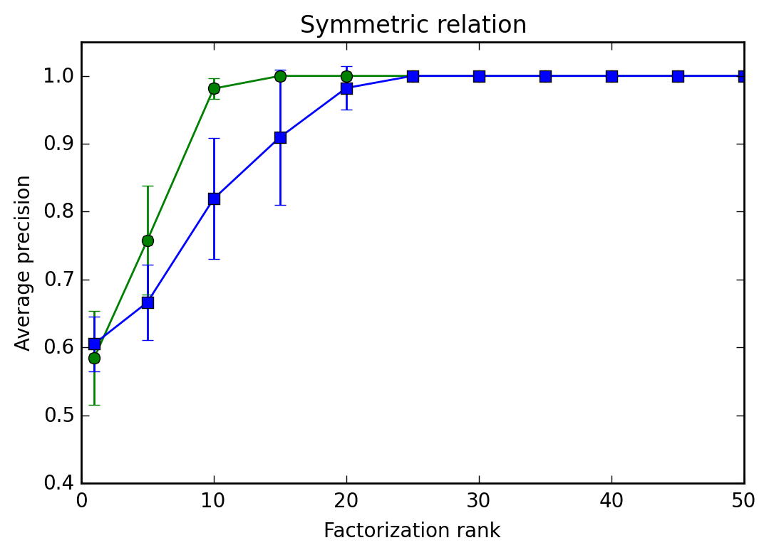
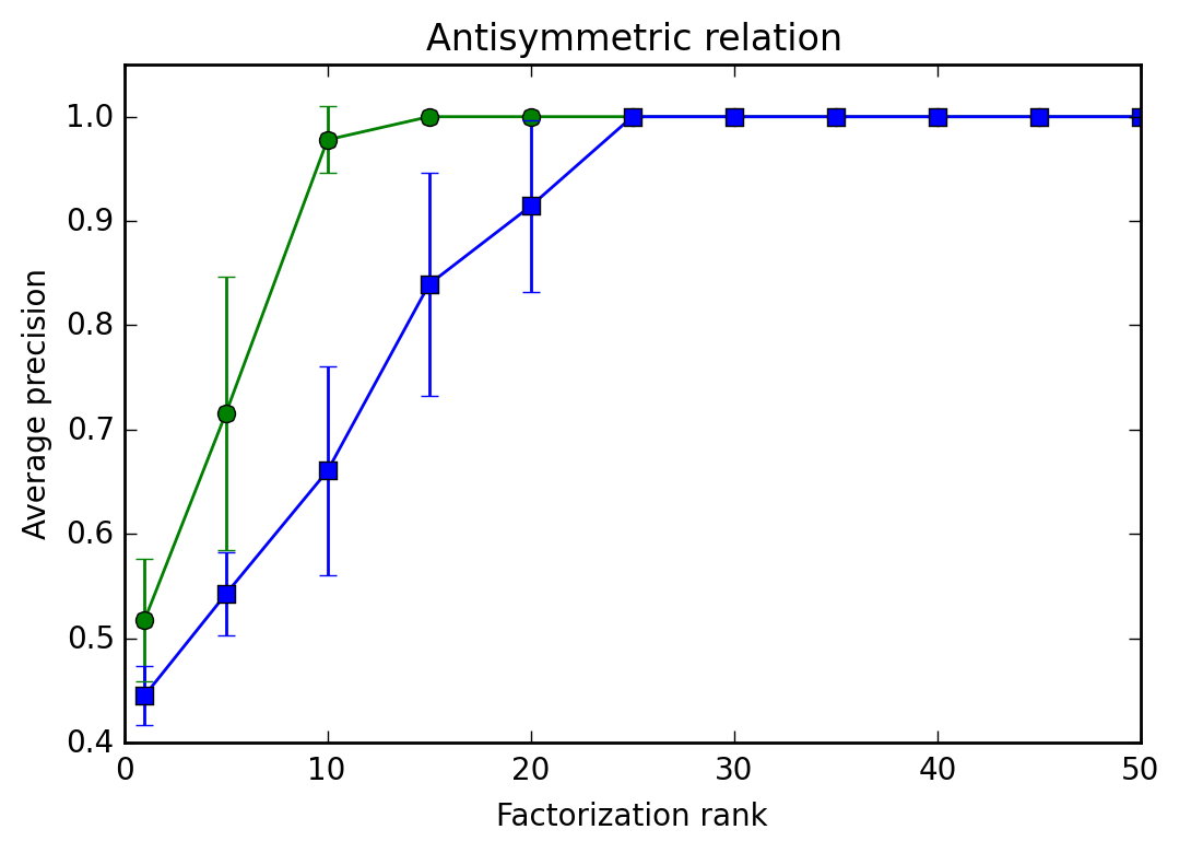
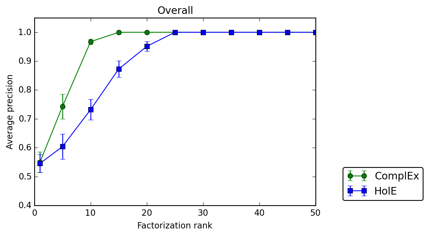
The results in Section 3 suggest that the choice of scoring function, i.e., ComplEx or HolE, does not affect the predictive abilities of the model. An additional important question is whether one of the models—in practice—is better suited for modeling certain types of relations. In particular, for symmetric relations, HolE needs to learn embeddings for which the imaginary part after the DFT is close to zero. ComplEx, on the other hand, can learn such representations easily as it operates directly in the complex domain. The question whether this difference in models translates to differences in practice affects the learning of both symmetric and antisymmetric relations. Relations $p\in\mathcal{R}$ are symmetric when triples have the same truth value by permutation of the subject and object entities: $y_{pso}=y_{pos}$ for all $s,o\in\mathcal{E}$, whereas facts of antisymmetric relations $p$ have inverse truth values: $y_{pso}=-y_{pos}$. To evaluate this question experimentally, we reproduced the joint learning of synthetic symmetric and antisymmetric relations described in Trouillon et al. [2016] on both scoring functions. We used the log-likelihood loss as all negatives are observed.

Figure 1: Average precision (AP) for each factorization rank ranging from 1 to 50 for the HolE and ComplEx scoring functions, with log-likelihood loss. Learning is performed jointly on the symmetric relation and on the antisymmetric relation. Top-left: AP over the symmetric relation only. Top-right: AP over the antisymmetric relation only. Bottom: Overall AP.

We generated randomly a $50\times 50$ symmetric matrix, and a $50\times 50$ antisymmetric matrix. Jointly, they represent a $2\times 50\times 50$ tensor. To ensure that all test values are predictable, the upper triangular parts of the matrices are always kept in the training set, and the diagonals are unobserved. We conducted 5-fold cross-validation on the lower-triangular matrices, using the upper-triangular parts plus 3 folds for training, one fold for validation and one fold for testing. The regularization parameter $\lambda$ is validated among the same values as in the previous experiment.

Figure 1 shows the best cross-validated average precision (area under the precision-recall curve) for the two scoring functions for ranks ranging up to 50. Both models manage to perfectly model symmetry and antisymmetry. As the ComplEx model has twice has many parameters for a given rank, it reaches a perfect average precision with a twice smaller rank. This confirms that the representation of the scoring function does not affect the learning abilities of the models in practice.

5 Discussion

We have demonstrated that the scoring functions of the HolE and ComplEx models are directly proportional. This hence extends the existence property of the ComplEx model over all knowledge graphs Trouillon et al. [2017] to the HolE model. We also showed experimentally that the difference between the reported results of the two models was due to the use of different loss functions, and specifically that the log-likelihood loss can produce a large improvement of predictive performances over the more often used margin loss. We have also shown that Complex and Holographic embeddings can be trained equally well on symmetric and antisymmetric patterns. All these things being equal, an interesting question is then in which settings one of the two models is preferable. Complex embeddings have an advantage in terms of time complexity as they scale linearly with the embedding dimension, whereas Holographic embeddings scale quasilinearly. An advantage of Holographic embeddings however is that the embeddings remain strictly in the real domain, which makes it easier for them to be used in other real-valued machine learning models. In contrast, Complex embeddings can not easily be transformed to real-valued vectors and used without loss of information—i.e. the specific way the real and imaginary parts interact in algebraic operations. Complex-valued models in which Complex embeddings can be directly input are emerging in machine learning Trabelsi et al. [2017]; Danihelka et al. [2016], but this path is yet to be explored for other relational learning problems. Hence, if the task of interest is link prediction, Complex embeddings offer an improved runtime complexity in the order of $O(\log K)$. If the embeddings should be used in further machine learning models, e.g. for entity classification, Holographic embeddings provide better compatibility with existing real-valued methods.

Furthermore, while the choice of the loss is of little consequence on the WN18 dataset, our experiments showed that the log-likelihood loss performed significantly better on FB15K. While much research attention has been given to scoring functions in link prediction, little has been said about the losses, and the max-margin loss has been used in most of the existing work Bordes et al. [2013]; Yang et al. [2015]; Riedel et al. [2013]. An interesting direction of future work is therefore a more detailed study of loss functions for knowledge graph embeddings—especially in light of the highly skewed label distribution and the open-world assumption which are characteristic for knowledge graphs but unusual for standard machine learning settings.

Appendix A Proof of Equivalence

In this section, we provide the full proof for the equivalence of both models. Note that a similar proof has recently been derived by Hayashi and Shimbo [2017].

We start from Equation 5 and show that there always exists corresponding real-valued holographic embeddings and complex embeddings such that the scoring functions of HolE and ComplEx are directly proportional, i.e. they are mathematically equal up to a constant multiplier $a\in\mathbb{R}$: $\phi^{h}_{pso}=a\phi^{c}_{pso}$. The key idea is in showing that the symmetry structure of vectors resulting from Fourier transform of real-valued vectors is such that, the trilinear product between these structured vectors is actually equal to keeping the real part of the trilinear product of their first half.

First, we derive a property of the DFT on real vectors $x$, showing that the resulting complex vector $\mathcal{F}(x)$ has a partially symmetric structure, for $j\in\{1,\ldots,K-1\}$:

$$\mathcal{F}(x)_{(K-j)} =\sum_{k=0}^{K-1}x_{k}e^{-2i\pi(K-j)\frac{k}{K}}$$

$$=\sum_{k=0}^{K-1}x_{k}e^{-2i\pi k}e^{2i\pi j\frac{k}{K}}$$

and given that $$k e^{-2i\pi k}=1$$ is an integer: ,

$$=\sum_{k=0}^{K-1}x_{k}e^{2i\pi j\frac{k}{K}}=\sum_{k=0}^{K-1}x_{k}\overline{e^{-2i\pi j\frac{k}{K}}}$$

and since $$x_{k}\in\mathbb{R}$$,

$$=\sum_{k=0}^{K-1}\overline{x_{k}e^{-2i\pi j\frac{k}{K}}}=\overline{\mathcal{F}(x)_{j}}\,.$$ (9)

Two special cases arise, the first one is $F(x)_{0}$, which is not concerned by the above symmetry property:

$$\mathcal{F}(x)_{0} =\sum_{k=0}^{K-1}x_{k}e^{-2i\pi 0\frac{k}{K}}$$

$$=\sum_{k=0}^{K-1}x_{k}=:s(x)\in\mathbb{R}\,.$$

And the second one is $F(x)_{\frac{K}{2}}$ when $K$ is even:

$$\mathcal{F}(x)_{(K-\frac{K}{2})} =\overline{\mathcal{F}(x)_{\frac{K}{2}}}=\mathcal{F}(x)_{\frac{K}{2}}$$

$$=\sum_{k=0}^{K-1}x_{k}e^{-2i\pi\frac{Kk}{2K}}=\sum_{k=0}^{K-1}x_{k}e^{-i\pi k}$$

$$=\sum_{k=0}^{\frac{K}{2}-1}x_{2k}-x_{2k+1}=:t(x)\in\mathbb{R}\,.$$

From Equations 9, LABEL:eq:f_0 and LABEL:eq:f_k/2, we write the general form of the Fourier transform $\mathcal{F}(x)\in\mathbb{C}^{K}$ of a real vector $x\in\mathbb{R}^{K}$:

$$\mathcal{F}(x)=\begin{cases}[s(x)\enspace x^{\prime}\enspace t(x)\enspace\overline{x^{\prime}}_{\leftarrow}],&\text{if}\ K\ \text{is even,}\\ [s(x)\enspace x^{\prime}\enspace\overline{x^{\prime}}_{\leftarrow}],&\text{if}\ K\ \text{is odd.}\end{cases}$$ (12)

where $x^{\prime},x^{\prime}_{\leftarrow}\in\mathbb{C}^{\left\lceil\frac{K}{2}\right\rceil-1}$, with $x^{\prime}=[\mathcal{F}(x)_{1},\ldots,\mathcal{F}(x)_{\left\lceil\frac{K}{2}\right\rceil-1}]$, and $x^{\prime}_{\leftarrow}$ is $x^{\prime}$ in reversed order: $x^{\prime}_{\leftarrow}=[\mathcal{F}(x)_{\left\lceil\frac{K}{2}\right\rceil-1},\ldots,\mathcal{F}(x)_{1}]$.

We can then derive Equation 6 for $r_{p},e_{s},e_{o}\in\mathbb{R}^{K}$, first with $K$ being odd:

$$\phi^{h}_{pso} =\frac{1}{K}\left<\mathcal{F}(r_{p}),\mathcal{F}(e_{s}),\overline{\mathcal{F}(e_{o})}\right>$$

$$=\frac{1}{K}\left<[s(r_{p})\enspace r^{\prime}_{p}\enspace\overline{r}^{\prime}_{p\leftarrow}],[s(e_{s})\enspace e^{\prime}_{s}\enspace\overline{e}^{\prime}_{s\leftarrow}],\overline{[s(e_{o})\enspace e^{\prime}_{o}\enspace\overline{e}^{\prime}_{o\leftarrow}]}\right>$$

$$=\frac{1}{K}\left<[s(r_{p})\enspace r^{\prime}_{p}\enspace\overline{r}^{\prime}_{p}],[s(e_{s})\enspace e^{\prime}_{s}\enspace\overline{e}^{\prime}_{s}],[s(e_{o})\enspace\overline{e}^{\prime}_{o}\enspace e^{\prime}_{o}]\right>$$

$$=\frac{1}{K}\left(s(r_{p})s(e_{s})s(e_{o})+\left<r^{\prime}_{p},e^{\prime}_{s},\overline{e}^{\prime}_{o}\right>+\left<\overline{r}^{\prime}_{p},\overline{e}^{\prime}_{s},e^{\prime}_{o}\right>\right)$$

$$=\frac{1}{K}\left(s(r_{p})s(e_{s})s(e_{o})+\left<r^{\prime}_{p},e^{\prime}_{s},\overline{e}^{\prime}_{o}\right>+\overline{\left<r^{\prime}_{p},e^{\prime}_{s},\overline{e}^{\prime}_{o}\right>}\right)$$

$$=\frac{1}{K}\left(s(r_{p})s(e_{s})s(e_{o})+2\,\left({\left<r^{\prime}_{p},e^{\prime}_{s},\overline{e}^{\prime}_{o}\right>}\right)\right)$$

$$=\frac{2}{K}\left(\left<\left[\sqrt[3]{\tfrac{1}{2}}s(r_{p})\enspace r^{\prime}_{p}\right],\left[\sqrt[3]{\tfrac{1}{2}}s(e_{s})\enspace e^{\prime}_{s}\right],\left[\sqrt[3]{\tfrac{1}{2}}s(e_{o})\enspace\overline{e}^{\prime}_{o}\right]\right>\right)$$

$$=\frac{2}{K}\left({\left<r^{\prime\prime}_{p},e^{\prime\prime}_{s},\overline{e}^{\prime\prime}_{o}\right>}\right)$$

$$=\frac{2}{K}\phi^{c}_{pso}\,$$ (13)

where $r^{\prime\prime}_{p},e^{\prime\prime}_{s},e^{\prime\prime}_{o}\in\mathbb{C}^{\left\lceil\frac{K}{2}\right\rceil}$. The derivation is similar when $K$ is even, with double prime vectors being $x^{\prime\prime}=[\sqrt[3]{\tfrac{1}{2}}s(x)\enspace\sqrt[3]{\tfrac{1}{2}}t(x)\enspace x^{\prime}]\in\mathbb{C}^{\frac{K}{2}+1}$.

As mentioned in Section 2, the complex vectors $r^{\prime\prime}_{r},e^{\prime\prime}_{s},e^{\prime\prime}_{o}\in\mathbb{C}^{\left\lceil\frac{K}{2}\right\rceil}$ equivalent to the real vectors $r_{p},e_{s},e_{o}\in\mathbb{R}^{K}$ are twice smaller, but take twice as much memory as real-valued ones of same size at a given floating-point precision. Both models hence have the exact same memory complexity.

References

- Bordes et al. [2013] Bordes, A.; Usunier, N.; Garcia-Duran, A.; Weston, J.; and Yakhnenko, O. 2013. Translating embeddings for modeling multi-relational data. In Advances in Neural Information Processing Systems, 2787–2795.
- Bordes et al. [2014] Bordes, A.; Glorot, X.; Weston, J.; and Bengio, Y. 2014. A semantic matching energy function for learning with multi-relational data. Machine Learning 94(2):233–259.
- Danihelka et al. [2016] Danihelka, I.; Wayne, G.; Uria, B.; Kalchbrenner, N.; and Graves, A. 2016. Associative long short-term memory. arXiv preprint arXiv:1602.03032.
- Duchi, Hazan, and Singer [2011] Duchi, J.; Hazan, E.; and Singer, Y. 2011. Adaptive subgradient methods for online learning and stochastic optimization. Journal of Machine Learning Research 12:2121–2159.
- Hayashi and Shimbo [2017] Hayashi, K., and Shimbo, M. 2017. On the equivalence of holographic and complex embeddings for link prediction. arXiv preprint arXiv:1702.05563.
- Nickel, Rosasco, and Poggio [2016] Nickel, M.; Rosasco, L.; and Poggio, T. A. 2016. Holographic embeddings of knowledge graphs. In AAAI Conference on Artificial Intelligence, 1955–1961.
- Riedel et al. [2013] Riedel, S.; Yao, L.; McCallum, A.; and Marlin, B. M. 2013. Relation extraction with matrix factorization and universal schemas. In Human Language Technologies: Conference of the North American Chapter of the Association of Computational Linguistics, 74–84.
- Trabelsi et al. [2017] Trabelsi, C.; Bilaniuk, O.; Serdyuk, D.; Subramanian, S.; Santos, J. F.; Mehri, S.; Rostamzadeh, N.; Bengio, Y.; and Pal, C. J. 2017. Deep complex networks. arXiv preprint arXiv:1705.09792.
- Trouillon et al. [2016] Trouillon, T.; Welbl, J.; Riedel, S.; Gaussier, E.; and Bouchard, G. 2016. Complex embeddings for simple link prediction. In International Conference on Machine Learning, volume 48, 2071–2080.
- Trouillon et al. [2017] Trouillon, T.; Dance, C. R.; Welbl, J.; Riedel, S.; Gaussier, É.; and Bouchard, G. 2017. Knowledge graph completion via complex tensor factorization. arXiv preprint arXiv:1702.06879, to appear in the Journal of Machine Learning Research.
- Yang et al. [2015] Yang, B.; Yih, W.-T.; He, X.; Gao, J.; and Deng, L. 2015. Embedding entities and relations for learning and inference in knowledge bases. In International Conference on Learning Representations.