Multiscale anisotropic fluctuations in sheared turbulence with multiple states

Abstract

We use high resolution direct numerical simulations to study the anisotropic contents of a turbulent, statistically homogeneous flow with random transitions among multiple energy containing states. We decompose the velocity correlation functions on different sectors of the three dimensional group of rotations, $SO(3)$, using a high-precision quadrature. Scaling properties of anisotropic components of longitudinal and transverse velocity fluctuations are accurately measured at changing Reynolds numbers. We show that independently of the anisotropic content of the energy containing eddies, small-scale turbulent fluctuations recover isotropy and universality faster than previously reported in experimental and numerical studies. The discrepancies are ascribed to the presence of highly anisotropic contributions that have either been neglected or measured with less accuracy in the foregoing works. Furthermore, the anomalous anisotropic scaling exponents are devoid of any sign of saturation with increasing order. Our study paves the way to systematically assess persistence of anisotropy in high Reynolds number flows.

The notion that all turbulent flows attain universal properties at small scales, regardless of the macroscopic details, has been an enduring and yet unproved concept in turbulence research Kolmogorov (1941a); Frisch (1995); Pope (2000). The energy containing scales in many flows such as shear, rotation, natural convection, thick layers, atmospheric boundary layer and magneto-hydrodynamic flows, are all strongly affected by anisotropic (and non-homogeneous) effects of the extrinsic stirring and boundary conditions, resulting in seemingly different flow configurations Dhruva et al. (1997); Godeferd and Moisy (2015); H. Xia, D. Byrne, G. Falkovich and M. Shats (2011); Saint-Michel et al. (2013); Gualtieri et al. (2013); Cambon et al. (2013); McCaffrey et al. (2015); Murphy and Pessah (2015); Liu et al. (2016); Sukoriansky and Galperin (2016). As such, anisotropic fluctuations are always connected to some degree of non-universality, i.e. dependency on the empirical setup. Can we disentangle anisotropic from isotropic statistical contributions? Are there any universal facets of turbulence? How does the relative importance of anisotropic and isotropic fluctuations vary with turbulence intensity? These are the questions we attempt to address.

On one hand, all phenomenological turbulence theories point toward a return-to-isotropy, at small enough scales Kolmogorov (1941a); Frisch (1995); Pope (2000). On the other hand, measurements of anisotropic contributions as functions of scale separation has revealed persistent small-scale anisotropy in hydrodynamical turbulence Tavoularis and Corrsin (1981); Pumir and Shraiman (1995); Garg and Warhaft (1998); Shen and Warhaft (2000); Warhaft and Shen (2002), magneto-hydrodynamics Müller et al. (2003); Watson et al. (2004), and passive scalar mixing Warhaft (2000); Biferale and Procaccia (2005). The persistence of anisotropy as reported in Refs. Garg and Warhaft (1998); Shen and Warhaft (2000); Warhaft (2000), was later reconciled with the postulate of local isotropy as an effect of the existence of anomalous scaling in both isotropic and anisotropic correlation functions Biferale and Vergassola (2001); Biferale and Procaccia (2005).

In this letter, we investigate the return-to-isotropy vs persistence-of-anisotropy, using direct numerical simulations (DNS) of turbulent flows subject to large-scale shear at high Reynolds numbers, $Re\equiv u^{\prime}r_{f}/\nu$, where $r_{f}$ denotes the typical forcing scale, $u^{\prime}$ the root-mean-square velocity fluctuation and $\nu$ is the viscosity. We use an exact decomposition of multi-point turbulent correlation functions in the eigen-basis of the $SO(3)$ group of rotations, which is the only systematic method to disentangle isotropic from anisotropic contributions, and to further distinguish among different anisotropic turbulent fluctuations. However, the utility of the $SO(3)$ decomposition has largely been impeded by practical difficulties in both experiments and simulations. High-Reynolds number experiments are beset with limitations on the set of directions that can be probed in three-dimensional (3D) space and consequently resort to ad-hoc curve fits to separate isotropic from anisotropic scaling properties Arad et al. (1998). Similarly, simulations have until now managed to perform the $SO(3)$ decomposition at low Reynolds numbers only Biferale and Procaccia (2005), due to computational bottlenecks (see Supplemental Material at SM for an estimate). Consequently, until now results concerning the multi-scale statistical properties of anisotropic fluctuations have been characterized by considerable scatter, thus calling into question their universal nature and in some instances even jeopardizing the fundamental postulate of small-scale isotropy Warhaft and Shen (2002).

The main features of this work are the following: First, we have achieved sufficiently high Reynolds numbers for a paradigmatic homogeneous shear configuration obtained from a random Kolmogorov Flow (RKF). Second, we have adopted a highly accurate Lebedev quadrature Lebedev (1975, 1976) for expanding the correlation functions in the irreducible representations of the $SO(3)$ symmetry group. On a $N^{3}$ grid, the new $SO(3)$ algorithm reduces the computational complexity from $\sim O(N^{6})$ to $\sim O(N^{3}\log N)$, thus expanding the range of problems where the $SO(3)$ decomposition can be viable (see Supplemental Material at SM for details, also see Pekurovsky (2012); Frigo and Johnson (2005)).

$R_{\lambda}$	$N$	${k_{max}\eta}$	${\mathbf{k}}_{1}$	${\mathbf{k}}_{2}$	$FT_{E}/u^{\prime}$	$T_{\textrm{tot}}/T_{E}$
$290$	$1024$	$1.94$	$\pm(2,0,0)$	$\pm(1,0,0)$	$0.48$	$118$
$450$	$2048$	$1.92$	$\pm(2,0,0)$	$\pm(1,0,0)$	$0.45$	$50$

Table 1: DNS parameters: Taylor scale Reynolds number $R_{\lambda}=\sqrt{20Re/3}$, resolution $N^{3}$, ${k_{max}\eta}=N\eta/3$ where $\eta=(\nu^{3}/\epsilon)^{1/4}$ is the Kolmogorov length scale and $\epsilon$ the mean dissipation, ${\mathbf{k}}_{1}$, ${\mathbf{k}}_{2}$ are the wave-vectors forced, $FT_{E}/u^{\prime}$ is the non-dimensional shear rate, where $F$ is the anisotropic forcing amplitude and $T_{\textrm{tot}}/T_{E}$ is the length of the stationary state simulation in multiples of large-eddy turnover time $T_{E}$.

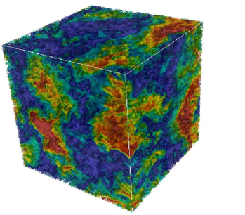
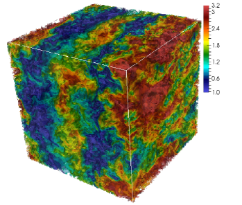
We discover that the flow evolution reveals unexpected bi-modal statistics of the energy containing scale, characterized by chaotic oscillations between two states, $I_{+}$ and $I_{-}$, corresponding to predominantly one-component (1C) and two-component (2C) axisymmetric macrostates (see 3D rendering in Fig. 1), respectively. We exploit the existence of the two macrostates in assessing universality as a function of the large-scale flow configurations. The main results are the following. (i) By going to smaller and smaller scales, isotropy is recovered faster than previously thought. We argue that this is due to the existence of non vanishing anisotropic contributions from the $j=4$ sector (see below) discarded or incorrectly measured in previous works Kurien and Sreenivasan (2000); Warhaft and Shen (2002); Biferale and Toschi (2001). (ii) We show that the anisotropic fluctuations of longitudinal and transverse velocity increments scale similarly. We confirm the theoretical expectation that all non-universal contributions are hidden in the power-law prefactors, sector-by-sector in the $SO(3)$ decomposition of the velocity correlations. (iii) The anisotropic scaling properties, contrary to previous expectations based on low Reynolds number calculations, do not saturate at higher orders, that they are universal and Reynolds independent at least up to the values investigated here.

We study the RKF Biferale and Toschi (2001) by evolving the 3D incompressible Navier-Stokes equations in a tri-periodic domain,

$$\partial\mathbf{u}/\partial t+\mathbf{u}\cdot\nabla\mathbf{u}=-\nabla p/\rho+\nu\nabla^{2}\mathbf{u}+\mathbf{f}\;,$$ (1)

where $p$ is the pressure and $\rho$ is the constant density. An anisotropic and statistically stationary state is attained by forcing only two wavenumbers (see Tab. 1) in the $y$-direction, $f_{y}(\mathbf{x},t)\!=\!F[\tilde{f_{y}}({\mathbf{k}}_{1},t)e^{i{\mathbf{k}}_{1}\cdot\mathbf{x}}\!+\!\tilde{f_{y}}({\mathbf{k}}_{2},t)e^{i{\mathbf{k}}_{2}\cdot\mathbf{x}}]$, where $F$ is a constant amplitude and the Fourier coefficients $\tilde{f}_{y}({\mathbf{k}}_{1,2},t)$ follow independent divergence-less Ornstein-Uhlenbeck processes Biferale et al. (2016). At variance with the standard non-homogeneous Kolmogorov Flow Borue and Orszag (1996), we recover translation invariant statistics by averaging the random forcing phases over multiple large-eddy turnover times, $T_{E}\equiv r_{f}/u^{\prime}$.

Figure 1: Evolution of $I_{3},I_{2}$ in the Lumley triangle (${\color[rgb]{1,0,0}\definecolor[named]{pgfstrokecolor}{rgb}{1,0,0}\times}$) for the $2048^{3}$ RKF. The laminar state given by the forcing configuration is shown by (${\color[rgb]{1,0,1}\definecolor[named]{pgfstrokecolor}{rgb}{1,0,1}\pgfsys@color@cmyk@stroke{0}{1}{0}{0}\pgfsys@color@cmyk@fill{0}{1}{0}{0}\blacktriangle}$). Inset shows steady-state evolution of $I_{2}$ $({\color[rgb]{0,0,1}\definecolor[named]{pgfstrokecolor}{rgb}{0,0,1}+})$ and $I_{3}$ $({\color[rgb]{0.65,0.16,0.16}\definecolor[named]{pgfstrokecolor}{rgb}{0.65,0.16,0.16}\ast})$ as functions of $t/T_{E}$. Reference line at zero is the isotropic state. Typical isocontours of the velocity magnitude in the 1C $(I_{+})$ and 2C $(I_{-})$ regions are also shown.

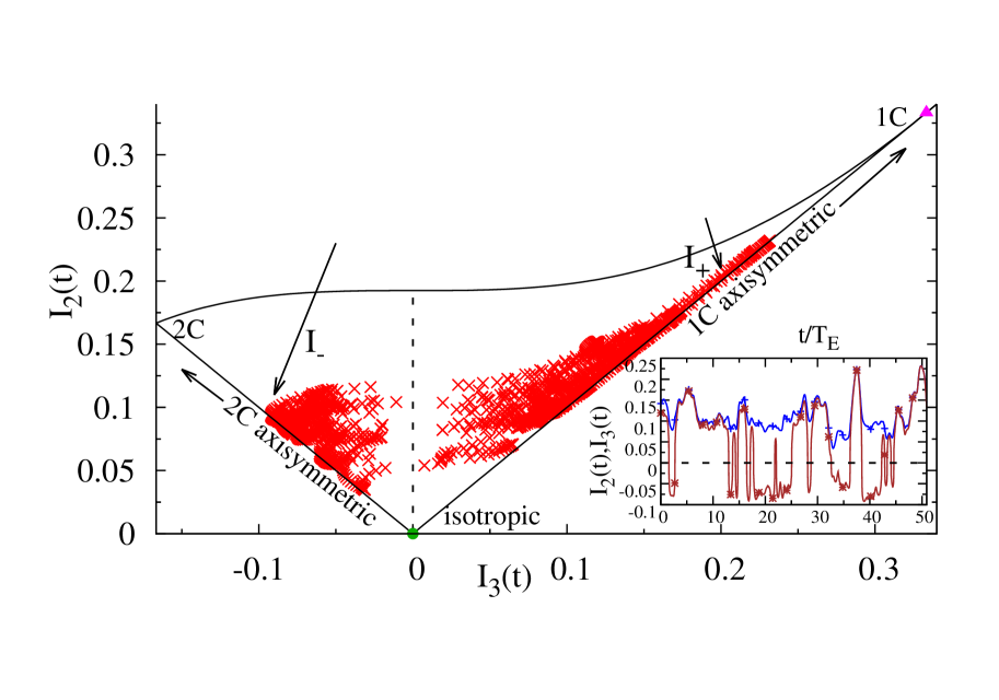
To quantify the anisotropy in the energy containing scales we examine the temporal evolution of the two invariants $I_{2}(t)=(b_{ij}b_{ji}/6)^{1/2},I_{3}(t)=(b_{ij}b_{jk}b_{ki}/6)^{1/3}$ of the Reynolds stress, $b_{ij}=(\langle u_{i}u_{j}\rangle/\langle u_{k}u_{k}\rangle)-\delta_{ij}/3$ Choi and Lumley (2001). Figure 1 shows $I_{2}$ plotted against $I_{3}$ at different time instants, in the Lumley triangle Lumley and Newman (1977). Surprisingly enough, despite the high Reynolds number, the dynamics is attracted by two different anisotropic axisymmetric states $I_{+}$ and $I_{-}$ where $I_{3}>0$ and $I_{3}<0$ respectively. The isocontours of the kinetic energy magnitude reveal a stark contrast in the large scale structures between the 1C and the 2C macrostates (see Fig. 1). The transition between $I_{+}$ and $I_{-}$ occurs suddenly during the time evolution, as shown in the inset of the same figure by the temporal evolution of the two invariants. Notice that the large scale configurations always avoid the isotropic $I_{2}=I_{3}=0$ state. The oscillations in the Reynolds stress suggest the existence of multiple turbulent states akin to those found in Taylor-Couette and Von Karman swirling flows Huisman, S. G. and van der Veen, R. C. A. and Sun, C. and Lohse, D. (2014); B. Saint-Michel, B. Dubrulle, L. Marié, F. Ravelet and F. Daviaud (2014); S. Thalabard, B. Saint-Michel, E. Herbert, F. Daviaud and B. Dubrulle (2015). Here, to assess the degree of small-scale universality at changing the large-scale anisotropy we will show results conditioned on the sign of $I_{3}$.
The longitudinal and transverse velocity increments are defined as ${\delta}u_{L}(\mathbf{x},\mathbf{r})\equiv{\delta}\mathbf{u}(\mathbf{x},\mathbf{r})\cdot{\hat{\mathbf{r}}}$ and ${\delta}\mathbf{u}_{T}(\mathbf{x},\mathbf{r})\equiv{\delta}\mathbf{u}(\mathbf{x},\mathbf{r})-{\delta}u_{L}(\mathbf{x},\mathbf{r})\hat{\mathbf{r}}$ respectively, where ${\delta}\mathbf{u}(\mathbf{x},\mathbf{r})\equiv\mathbf{u}(\mathbf{x}+\mathbf{r})-\mathbf{u}(\mathbf{x})$ is the two-point velocity difference at separation vector $\mathbf{r}$ and $\hat{\mathbf{r}}$ is the unit vector along $\mathbf{r}$. The $p^{\textrm{th}}$ order longitudinal structure function (LSF) and transverse structure function (TSF), are

$$S^{(p,L)}(\mathbf{r}) \equiv \langle({\delta}u_{L}(\mathbf{x},\mathbf{r}))^{p}\rangle\;,$$ (2)

$$S^{(p,T)}(\mathbf{r}) \equiv \langle({\delta}\mathbf{u}_{T}(\mathbf{x},\mathbf{r})\cdot{\delta}\mathbf{u}_{T}(\mathbf{x},\mathbf{r}))^{p/2}\rangle\;,$$ (3)

where $\langle\cdot\rangle$ denotes space and time averages. Since $S^{(p,L)}(\mathbf{r})$ are scalar functions of a vector arguments, they can be expanded in spherical harmonics $Y_{jm}(\hat{\mathbf{r}})$ Arad et al. (1999) as,

$$S^{(p,L)}(\mathbf{r})=\sum^{\infty}_{j=0}\sum_{m=-j}^{m=+j}S^{(p,L)}_{j,m}(r)Y_{jm}(\hat{\mathbf{r}})\;.$$ (4)

The index $j$ labels the different degrees of anisotropy, while the dependency on $m$ distinguishes different degrees of freedom within a given anisotropic sector. The TSF can be expanded similarly via the corresponding projections $S^{(p,T)}_{j,m}$. The projection on the $j=0$ sector corresponds to the isotropic case, the only one that will survive if the external forcing is invariant under rotation. Theoretical speculations suggest that at high enough $Re$ and for small enough scales $r\ll r_{f}$, a foliation of the physics in different $j$-sectors occurs, characterized by different power law scaling Kurien and Sreenivasan (2001); Biferale and Procaccia (2005),

$$\!\!\!\!S^{(p,L)}_{j,m}(r)\!\!=\!\!\Lambda^{(p,L)}_{j,m}\!\Big{(}{\frac{r}{r_{f}}}\Big{)}^{{{{\xi}^{L}_{j}}(p)}}\!\!;S^{(p,T)}_{j,m}(r)\!\!=\!\!\Lambda^{(p,T)}_{j,m}\!\Big{(}{\frac{r}{r_{f}}}\Big{)}^{{{{\xi}^{T}_{j}}(p)}}\!\!\!.$$ (5)

Figure 2: Log-log plot of $|S^{(3,L)}_{j,m}|$ vs $r$ for different $(j,m)$ sectors at $R_{\lambda}=450$. Symbols correspond to sectors $(0,0)$ $({\color[rgb]{0,0.5,0}\definecolor[named]{pgfstrokecolor}{rgb}{0,0.5,0}\square})$, $(2,0)$ $({\color[rgb]{1,0,0}\definecolor[named]{pgfstrokecolor}{rgb}{1,0,0}\circ})$, $(4,4)$ $({\color[rgb]{0,0,1}\definecolor[named]{pgfstrokecolor}{rgb}{0,0,1}\triangle})$ and $(6,6)$ $({\color[rgb]{1,0,1}\definecolor[named]{pgfstrokecolor}{rgb}{1,0,1}\pgfsys@color@cmyk@stroke{0}{1}{0}{0}\pgfsys@color@cmyk@fill{0}{1}{0}{0}\triangledown})$, respectively. Inset shows corresponding logarithmic local slopes for sectors $(0,0)$ and $(4,4)$ at $R_{\lambda}=300$ (closed symbols) and $R_{\lambda}=450$ (open symbols). Horizontal line at $1.0$ is the exact result for sector $(0,0)$ Kolmogorov (1941b).

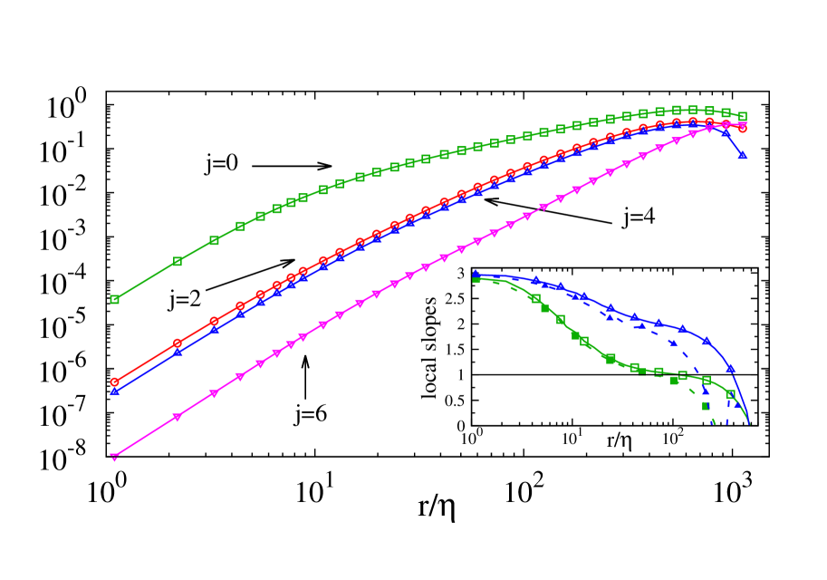
All questions can then be translated in terms of the above defined quantities. Recovery of isotropy (universality) implies that a strict hierarchy exists among the isotropic and anisotropic exponents, $\xi^{L}_{0}(p)<\xi^{L}_{j>0}(p)$. The rate of recovery being measured by the gap between the exponents of the same order: smaller the gap, slower the anisotropic contributions decay. Theoretical considerations suggest that the exponents ${{{\xi}^{L}_{j}}(p)}$ and ${{{\xi}^{T}_{j}}(p)}$ are universal, i.e. independent of the large-scale configuration. The prefactors $\Lambda^{(p,L)}_{j,m}$ and $\Lambda^{(p,T)}_{j,m}$ must be non-universal being determined by the matching for $r\sim r_{f}$. The exact expansion (4) together with scaling assumption (5) imply that in presence of anisotropy, multiple power laws are present in the undecomposed correlations such as $S^{(p,L)}(\mathbf{r})$ and hence non-trivial, sub-leading terms can contaminate their scaling behaviour. Conversely, the projected components $S^{(p,L)}_{j,m}$, must show a pure power law behaviour. In Fig. 2 we asses the rate of recovery-of-isotropy by plotting the magnitudes $|S^{(p,L)}_{j,m}(r)|$ for $p=3$, up to $j=6$ (we omit those $(j,m)$ sectors that have negligible intensity or that have similar scaling properties). All projections exhibit a clear power-law behavior. The isotropic projection scales quasilinearly in the scale range $44\leq r/\eta\leq 350$, as it does in an isotropic flow, due to the $4/5$th law Kolmogorov (1941b); Qian (1997); Lundgren (2002). All sectors have comparable magnitude at the forcing scale, confirming the strong anisotropy of the energy containing scales. In contrast, the anisotropic projections become more and more sub-leading with decreasing $r$. The quality of the scaling properties are shown in the inset of Fig. 2 where we compare the logarithmic derivatives of $j=0$ and $j=4$ at two different Reynolds numbers. Similar plots are obtained for other moments and for transverse increments (see also later). It is important to stress that the anisotropic projections shown in Fig. 2 display a quality of scaling never achieved before concerning both statistical accuracy and extension of the inertial range of scales. An extremely high numerical and statistical accuracy is required to disentangle fluctuations that differ up to four orders of magnitude (compare sectors $j=6$ and $j=0$ at the smallest $r$). These results have been possible due to the highly accurate quadrature that has been used for the $SO(3)$ decomposition (see Supplemental Material at SM for details).

Figure 3: Lin-log plot of undecomposed compensated structure function $-5S^{(3,L)}(\mathbf{r})/4r\epsilon$ at $R_{\lambda}=450$ along the Cartesian directions, $\hat{x}$ $({\color[rgb]{1,0,0}\definecolor[named]{pgfstrokecolor}{rgb}{1,0,0}\circ})$, $\hat{y}$ $({\color[rgb]{0,0,1}\definecolor[named]{pgfstrokecolor}{rgb}{0,0,1}\triangle})$ and $\hat{z}$ $({\color[rgb]{1,0,1}\definecolor[named]{pgfstrokecolor}{rgb}{1,0,1}\pgfsys@color@cmyk@stroke{0}{1}{0}{0}\pgfsys@color@cmyk@fill{0}{1}{0}{0}\diamond})$. The corresponding projection on the isotropic sector, $-5S^{(3,L)}_{(0,0)}(r)Y_{00}/4r\epsilon$ is given by $({\color[rgb]{0,0.5,0}\definecolor[named]{pgfstrokecolor}{rgb}{0,0.5,0}\blacksquare})$. Inertial range (IR) is taken as that range within $5\%$ of the exact IR result, shown by the dashed line at unity.

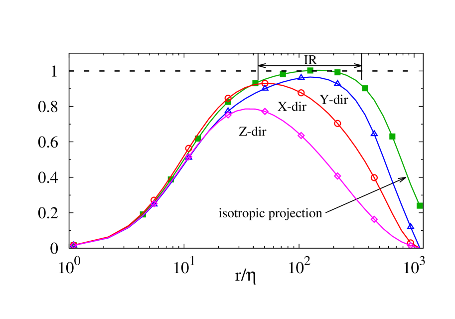
Despite anisotropies being sub-leading at the small scales, their cumulative effects are important and strongly influence scaling laws if not properly decomposed. This is shown in Fig. 3 which compares the undecomposed third order LSF along the three Cartesian directions along with the projection on the isotropic sector, all compensated with the exact isotropic $4/5$th linear behaviour, $-4/5\epsilon r$. The undecomposed correlations do not compensate well and depend on the chosen direction. In contrast, the isotropic sector confirms the K41 plateau Kolmogorov (1941b) on a wide range of scales(Taylor et al., 2003).

Figure 4: (a): log-log plot of $S^{(p,L)}_{j,m}\big{|}_{I_{+}}$ vs. $S^{(p,L)}_{j,m}\big{|}_{I_{-}}$ at various orders $p$ and sectors $(j,m)$. (b): the same but for transverse structure functions. Universality with respect to large scale conditioning corresponds to slope $1$ as shown by the dashed straight lines. For clarity, curves are offset upwards.

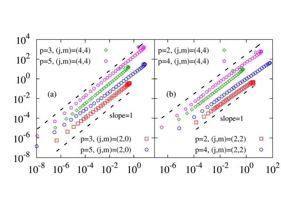
To assess universality of the scaling properties sector-by-sector, we show in Fig. 4 that both $S^{(p,L)}_{j,m}$ (left panel) and $S^{(p,T)}_{j,m}$ (right panel) scale similarly when conditioned on $I_{+}$ or $I_{-}$ events. Using a least-square fit we find that the relative scaling exponents for all curves is $\sim 1$ within $5\%$. This supports the foliation argument that the scaling exponents, sector-wise are immune to anisotropic large scale effects and are hence universal.

Figure 5: Summary of scaling exponents of $S^{(p,L)}_{j,m}$ (open symbols) and $S^{(p,T)}_{j,m}$ (closed symbols) vs order $p$ for sectors $j\leq 6$. Error bars indicate $95\%$ confidence intervals. Data from experiments for $j=2$ $(\ast)$ given for comparison Kurien and Sreenivasan (2000); Warhaft and Shen (2002).

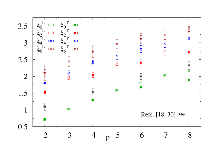
The summary for all scaling exponents of different LSF and TSF projections on the different sectors are plotted for various orders in Fig. 5. A few final comments are in order. (i) Both ${{{\xi}^{L}_{j}}(p)}$ and ${{{\xi}^{T}_{j}}(p)}$ have similar values, except for small deviations at orders $p\geq 6$ in the $j=0$ sector (see Refs. Chen et al. (1997); Benzi et al. (2010); Iyer et al. (2017) for a discussion on the Reynolds number dependency of the isotropic exponents). (ii) At any given order $p$, a finite gap exists between isotropic and anisotropic exponents, indicating a strict asymptotic recovery of isotropy for the whole probability distribution function. (iii) For any $j$, the scaling exponents do not scale linearly in $p$, contrary to the dimensional prediction ${{{\xi}_{j,dim}}(p)}=(p+j)/3$ proposed in Ref. Biferale et al. (2002), indicating that anomalous scaling is also present in $j>0$ sectors. Importantly enough, the new $SO(3)$ scheme using a high order Lebedev rule (Lebedev and Laikov, 1999; jbu, ) enables us to clean the previously reported results. For example, in contrast to Ref. Biferale and Toschi (2001), we find that the exponents in any given anisotropic sector increase with order $p$ with no apparent saturation. We contend that the saturation observed in Ref. Biferale and Toschi (2001) is due to spurious effects induced by combination of poor accuracy in the $SO(3)$ expansion and potential contamination by hyper-viscous effects. In Fig. 5 we also report results for the $j=2$ sector from the few prior experiments Kurien and Sreenivasan (2000); Warhaft and Shen (2002). In experiments, it is difficult to perform measurements along a sufficiently large number of directions to adequately resolve the anisotropic fluctuations on the $2$-sphere, in contrast $\sim O(1000)$ different directions were used in this work. As a result, experiments must resort to a fit for the entire right-hand-side of Eq. 4 using data along a few directions only. In order to reduce the number of fitting parameters the sum on all sectors is typically cut at $j=2$, something that is clearly not enough in view of the results shown in Fig. 2. Indeed, we find that sector $j=4$ is almost as energetic as $j=2$, with a very similar scaling exponent, i.e. the $j=4$ contribution is as important as $j=2$, at almost all scales. Figure 5 shows that the results from our exact decomposition clearly differ with that of Refs. Kurien and Sreenivasan (2000); Warhaft and Shen (2002), wherein sectors $j\geq 4$ are neglected. In the presence of many anisotropic sectors, obtaining scaling exponents by assuming that only the lowest anisotropic sector is dominant can strongly affect the measured rate of return owing to spurious cancellations. Only the exact $SO(3)$ expansion allows the measurement of $\xi_{j}(p)$, devoid of contamination from sectors $j^{\prime}\neq j$, thus yielding a true gauge of the rate of return at a given order $p$. It remains to be clarified if in the homogeneous shear case analyzed in Refs. Shen and Warhaft (2000); Warhaft and Shen (2002) the scaling properties of high order sectors $j\geq 4$ are also as important as in the RKF.
In conclusion, we have used an efficient algorithm for the $SO(3)$ decomposition, to study anisotropy in high Reynolds numbers Kolmogorov Flows. We have found that the RKF develops a two-state attractor characterized by very different anisotropic large scale contents. We have shown that the scaling exponents in RKF are immune to different large scale effects and hence are universal. The magnitude of the anisotropic exponents indicate that isotropy is recovered at a faster rate than previously thought. Nevertheless, projection on the $SO(3)$ is mandatory to detect a clean scaling, since power laws exists only sector-by-sector. We do not observe saturation of exponents at the higher $j$-sectors, indicating that intense anisotropic fluctuations are dominated by more than one singular structure. Differently from previous observations, we demonstrate that it is mandatory to resolve at least up to sector $j=4$ to have clean scaling properties, sector by sector. We hope our study will stimulate further theoretical or phenomenological efforts to predict the scaling properties for all $j$-sectors. It will be important to extend this analysis to other turbulent flows, such as those in the presence of rotation, mean shear and magnetic field, in order to establish, on a firmer basis the degree of universality. The improvement provided by the fast $SO(3)$ solver opens the road to perform such studies.

I Acknowledgments

We thank Susan Kurien for useful discussions. We acknowledge funding from the European Research Council under the European Community’s Seventh Framework Program, ERC Grant Agreement No $339032$. The computations were performed using resources provided through the PRACE initiative $\textrm{Pra}11\textrm{\_}2870$ at the CINECA Consortium. We acknowledge the European COST Action MP1305 “Flowing Matter”.

References

- Kolmogorov (1941a) A. N. Kolmogorov, “Local structure of turbulence in an incompressible fluid for very large reynolds numbers,” Dokl. Akad. Nauk. SSSR 30, 299–303 (1941a).
- Frisch (1995) U. Frisch, Turbulence (Cambridge University Press, 1995).
- Pope (2000) S. B. Pope, Turbulent Flows (Cambridge University Press, 2000).
- Dhruva et al. (1997) B. Dhruva, Y. Tsuji, and K. R. Sreenivasan, “Transverse structure functions in high-reynolds-number turbulence,” Phys. Rev. E 56, R4928–R4930 (1997).
- Godeferd and Moisy (2015) F. S. Godeferd and F. Moisy, “Structure and dynamics of rotating turbulence: A review of recent experimental and numerical results,” ASME. Appl. Mech. Rev. 67 (2015).
- H. Xia, D. Byrne, G. Falkovich and M. Shats (2011) H. Xia, D. Byrne, G. Falkovich and M. Shats, “Upscale energy transfer in thick turbulent fluid layers,” Nature Phys. 7, 321–324 (2011).
- Saint-Michel et al. (2013) B. Saint-Michel, B. Dubrulle, L. Marié, F. Ravelet, and F. Daviaud, “Evidence for forcing-dependent steady states in a turbulent swirling flow,” Phys. Rev. Lett. 111, 234502 (2013).
- Gualtieri et al. (2013) P. Gualtieri, F. Picano, G. Sardina, and C. M. Casciola, “Clustering and turbulence modulation in particle-laden shear flows,” J. Fluid Mech. 715, 134–162 (2013).
- Cambon et al. (2013) C. Cambon, L. Danaila, F. S. Godeferd, and J. F. Scott, “Third-order statistics and the dynamics of strongly anisotropic turbulent flows,” J. Turb. 14, 121–160 (2013).
- McCaffrey et al. (2015) K. McCaffrey, B. Fox-Kemper, P. E. Hamlington, and J. Thomson, “Characterization of turbulence anisotropy, coherence, and intermittency at a prospective tidal energy site: Observational data analysis,” Renew. Energ. 76, 441–453 (2015).
- Murphy and Pessah (2015) G. C. Murphy and M. E. Pessah, “On the anisotropic nature of mri-driven turbulence in astrophysical disks,” Astrophys. J. 802, 139 (2015).
- Liu et al. (2016) C. C. Liu, R. T. Cerbus, and P. Chakraborty, “Janus spectra in two-dimensional flows,” Phys. Rev. Lett. 117, 114502 (2016).
- Sukoriansky and Galperin (2016) S. Sukoriansky and G. Galperin, “Qnse theory of turbulence anisotropization and onset of the inverse energy cascade by solid body rotation,” J. Fluid Mech. 805, 384–421 (2016).
- Tavoularis and Corrsin (1981) S. Tavoularis and S. Corrsin, “Experiments in nearly homogeneous turbulent shear flow with a uniform mean temperature gradient. part 2. the fine structure,” J. Fluid Mech. 104, 349–367 (1981).
- Pumir and Shraiman (1995) A. Pumir and B. I. Shraiman, “Persistent small scale anisotropy in homogeneous shear flows,” Phys. Rev. Lett. 75, 3114–3117 (1995).
- Garg and Warhaft (1998) S. Garg and Z. Warhaft, “On the small scale structure of simple shear flow,” Phys. Fluids 10, 662–673 (1998).
- Shen and Warhaft (2000) X. Shen and Z. Warhaft, “The anisotropy of the small scale structure in high Reynolds number () turbulent shear flow,” Phys. Fluids 12, 2976–2989 (2000).
- Warhaft and Shen (2002) Z. Warhaft and X. Shen, “On the higher order mixed structure functions in laboratory shear flow,” Phys. Fluids 14, 2432–2438 (2002).
- Müller et al. (2003) W. C. Müller, D. Biskamp, and R. Grappin, “Statistical anisotropy of magnetohydrodynamic turbulence,” Phys. Rev. E 67, 066302 (2003).
- Watson et al. (2004) W. D. Watson, D. S. Wiebe, J. C. McKinney, and C. F. Gammie, “Anisotropy of magnetohydrodynamic turbulence and the polarized spectra of oh masers,” Astrophys. J. 604, 707–716 (2004).
- Warhaft (2000) Z. Warhaft, “Passive scalars in turbulent flows,” Annu. Rev. Fluid Mech. 32, 203–240 (2000).
- Biferale and Procaccia (2005) L. Biferale and I. Procaccia, “Anisotropy in turbulent flows and in turbulent transport,” Phys. Rep. 414, 43–164 (2005).
- Biferale and Vergassola (2001) L. Biferale and M. Vergassola, “Isotropy vs anisotropy in small-scale turbulence,” Phys. Fluids 13, 2139–2141 (2001).
- Arad et al. (1998) I. Arad, B. Dhruva, S. Kurien, V. S. L’vov, I. Procaccia, and K. R. Sreenivasan, “The extraction of anisotropic contributions in turbulent flows,” Phys. Rev. Lett. 81, 5330–5333 (1998).
- (25) “Supplemental material,” .
- Lebedev (1975) V. I. Lebedev, “Values of the nodes and weights of ninth to seventeenth order gauss-markov quadrature formulae invariant under the octahedron group with inversion,” USSR Comp. Math. & Math. Phys. 15, 44–51 (1975).
- Lebedev (1976) V. I. Lebedev, “Quadratures on a sphere,” USSR Comp. Math. & Math. Phys. 16, 10–24 (1976).
- Pekurovsky (2012) D. Pekurovsky, “P3DFFT: A framework for parallel computations of Fourier transforms in three dimensions,” SIAM J. Sci. comp. , C192–C209 (2012).
- Frigo and Johnson (2005) M. Frigo and S. G. Johnson, “The design and implementation of FFTW3,” Proc. IEEE , 216–231 (2005), special issue on “Program Generation, Optimization, and Platform Adaptation”.
- Kurien and Sreenivasan (2000) S. Kurien and K. R. Sreenivasan, “Anisotropic scaling contributions to high-order structure functions in high-reynolds-number turbulence,” Phys. Rev. E 62, 2206 (2000).
- Biferale and Toschi (2001) L. Biferale and F. Toschi, “Anisotropic homogeneous turbulence: Hierarchy and intermittency of scaling exponents in the anisotropic sectors,” Phys. Rev. Lett. 86, 4831–4834 (2001).
- Biferale et al. (2016) L. Biferale, F. Bonaccorso, I. M. Mazzitelli, M. A. T. van Hinsberg, A. S. Lanotte, S. Musacchio, P. Perlekar, and F. Toschi, “Coherent structures and extreme events in rotating multiphase turbulent flows,” Phys. Rev. X 6, 041036 (2016).
- Borue and Orszag (1996) V. Borue and S. Orszag, “Numerical study of three-dimensional kolmogorov flow at high reynolds numbers,” J. Fluid Mech. 306, 293–323 (1996).
- Choi and Lumley (2001) K. S. Choi and J. L. Lumley, “The return to isotropy of homogenous turbulence,” J. Fluid Mech. 436, 59–84 (2001).
- Lumley and Newman (1977) J. L. Lumley and G. R. Newman, “The return to isotropy of homogenous turbulence,” J. Fluid Mech. 82, 161–178 (1977).
- Huisman, S. G. and van der Veen, R. C. A. and Sun, C. and Lohse, D. (2014) Huisman, S. G. and van der Veen, R. C. A. and Sun, C. and Lohse, D., “Multiple states in highly turbulent taylor–couette flow,” Nature Comm. 5, 3820EP (2014).
- B. Saint-Michel, B. Dubrulle, L. Marié, F. Ravelet and F. Daviaud (2014) B. Saint-Michel, B. Dubrulle, L. Marié, F. Ravelet and F. Daviaud, “Influence of Reynolds number and forcing type in a turbulent von Kármán flow,” New J. Phys. 16, 063037 (2014).
- S. Thalabard, B. Saint-Michel, E. Herbert, F. Daviaud and B. Dubrulle (2015) S. Thalabard, B. Saint-Michel, E. Herbert, F. Daviaud and B. Dubrulle, “A statistical mechanics framework for the large-scale structure of turbulent von Kármán flows,” New J. Phys. 17, 063006 (2015).
- Arad et al. (1999) I. Arad, V. S. L’vov, and I. Procaccia, “Correlation functions in isotropic and anisotropic turbulence: the role of the symmetry group,” Phys. Rev. E 59, 6753–6765 (1999).
- Kurien and Sreenivasan (2001) S. Kurien and K. R. Sreenivasan, “Measures of anisotropy and the universal properties of turbulence,” in New trends in turbulence: nouveaux aspects: 31 July – 1 September 2000, edited by M. Lesieur, A. Yaglom, and F. David (Springer Berlin Heidelberg, Berlin, Heidelberg, 2001) pp. 53–111.
- Kolmogorov (1941b) A. N. Kolmogorov, “Dissipation of energy in locally isotropic turbulence,” Dokl. Akad. Nauk. SSSR 434, 16–18 (1941b).
- Qian (1997) J. Qian, “Inertial range and the finite reynolds number effect of turbulence,” Phys. Rev. E 55, 337–342 (1997).
- Lundgren (2002) T. S. Lundgren, “Kolmogorov two-thirds law by matched asymptotic expansion,” Phys. Fluids 14, 638–642 (2002).
- Taylor et al. (2003) M. A. Taylor, Kurien S., and Eyink G. L., “Recovering isotropic statistics in turbulence simulations: The kolmogorov 4/5th law,” Phys. Rev. E 68, 026310 (2003).
- Chen et al. (1997) S. Chen, K. R. Sreenivasan, M. Nelkin, and N. Cao, “Refined similarity hypothesis for transverse structure functions in fluid turbulence,” Phys. Rev. Lett. 79, 2253–2256 (1997).
- Benzi et al. (2010) R. Benzi, L. Biferale, R. Fisher, D. Q. Lamb, and F. Toschi, “Inertial range eulerian and lagrangian statistics from numerical simulations of isotropic turbulence,” J. Fluid Mech. 653, 221–244 (2010).
- Iyer et al. (2017) K. P. Iyer, K. R. Sreenivasan, and P. K. Yeung, “Reynolds number scaling of velocity increments in isotropic turbulence,” Phys. Rev. E 95, 021101 (2017).
- Biferale et al. (2002) L. Biferale, I. Daumont, A. Lanotte, and F. Toschi, “Anomalous and Dimensional scaling in anisotropic turbulence,” Phys. Rev. E 66, 056306 (2002).
- Lebedev and Laikov (1999) V. I. Lebedev and D. N. Laikov, “A quadrature formula for the sphere of the 131st algebraic order of accuracy,” Dokl. Math. 59, 477–481 (1999).
- (50) https://people.sc.fsu.edu/~jburkardt/c_src/sphere_lebedev_rule/sphere_lebedev_rule.html.