Variation of the Nazarov-Sodin constant for random plane waves and arithmetic random waves

Pär Kurlberg  and  Igor Wigman
Abstract.

This is a manuscript containing the full proofs of results announced in  [KW], together with some recent updates. We prove that the Nazarov-Sodin constant, which up to a natural scaling gives the leading order growth for the expected number of nodal components of a random Gaussian field, genuinely depends on the field. We then infer the same for “arithmetic random waves”, i.e. random toral Laplace eigenfunctions.

1. Introduction

For m2𝑚2m\geq 2, let f:m:𝑓superscript𝑚f:\mathbb{R}^{m}\rightarrow\mathbb{R} be a stationary centred Gaussian random field, and rf:m:subscript𝑟𝑓superscript𝑚r_{f}:\mathbb{R}^{m}\rightarrow\mathbb{R} its covariance function

rf(x)=𝔼[f(0)f(x)]=𝔼[f(y)f(x+y)].subscript𝑟𝑓𝑥𝔼delimited-[]𝑓0𝑓𝑥𝔼delimited-[]𝑓𝑦𝑓𝑥𝑦r_{f}(x)=\mathbb{E}[f(0)\cdot f(x)]=\mathbb{E}[f(y)\cdot f(x+y)].

Given such an f𝑓f, let ρ𝜌\rho denote its spectral measure, i.e. the Fourier transform of rfsubscript𝑟𝑓r_{f} (assumed to be a probability measure); note that prescribing ρ𝜌\rho uniquely defines f𝑓f by Kolmogorov’s Theorem (cf. [CL, Chapter 3.3].) In what follows we often allow for ρ𝜌\rho to vary; it will be convenient to let fρsubscript𝑓𝜌f_{\rho} denote a random field with spectral measure ρ𝜌\rho. We further assume that a.s. fρsubscript𝑓𝜌f_{\rho} is sufficiently smooth, and that the distribution of f𝑓f and its derivatives is non-degenerate in an appropriate sense (a condition on the support of ρ𝜌\rho).

1.1. Nodal components and the Nazarov-Sodin constant

Let 𝒩(fρ;R)𝒩subscript𝑓𝜌𝑅\mathcal{N}(f_{\rho};R) be the number of connected components of fρ1(0)superscriptsubscript𝑓𝜌10f_{\rho}^{-1}(0) in B0(R)subscript𝐵0𝑅B_{0}(R) (the radius-R𝑅R ball centred at 00), usually referred to as the nodal components of fρsubscript𝑓𝜌f_{\rho}; 𝒩(fρ;R)𝒩subscript𝑓𝜌𝑅\mathcal{N}(f_{\rho};R) is a random variable. Assuming further that fρsubscript𝑓𝜌f_{\rho} is ergodic (equivalently, ρ𝜌\rho has no atoms), with non-degenerate gradient distribution (equivalent to ρ𝜌\rho not being supported on a hyperplane passing through the origin), Nazarov and Sodin [So, Theorem 111] evaluated the expected number of nodal components of fρsubscript𝑓𝜌f_{\rho} to be asymptotic to

(1.1) 𝔼[𝒩(fρ;R)]=cNS(ρ)Vol(B(1))Rm+o(Rm),𝔼delimited-[]𝒩subscript𝑓𝜌𝑅subscript𝑐𝑁𝑆𝜌Vol𝐵1superscript𝑅𝑚𝑜superscript𝑅𝑚\mathbb{E}[\mathcal{N}(f_{\rho};R)]=c_{NS}(\rho)\cdot\operatorname{Vol}(B(1))\cdot R^{m}+o(R^{m}),

where cNS(ρ)0subscript𝑐𝑁𝑆𝜌0c_{NS}(\rho)\geq 0 is a constant, subsequently referred to as the “Nazarov-Sodin constant” of fρsubscript𝑓𝜌f_{\rho}, and Vol(B(1))Vol𝐵1\operatorname{Vol}(B(1)) is the volume of the radius-111 m𝑚m-ball B(1)m𝐵1superscript𝑚B(1)\subseteq\mathbb{R}^{m}. They also established convergence in mean, i.e., that

(1.2) 𝔼[|𝒩(fρ;R)Vol(B(1))RmcNS(ρ)|]0;𝔼delimited-[]𝒩subscript𝑓𝜌𝑅Vol𝐵1superscript𝑅𝑚subscript𝑐𝑁𝑆𝜌0\mathbb{E}\left[\left|\frac{\mathcal{N}(f_{\rho};R)}{\operatorname{Vol}(B(1))\cdot R^{m}}-c_{NS}(\rho)\right|\right]\rightarrow 0;

it is a consequence of the assumed ergodicity of the underlying random field fρsubscript𝑓𝜌f_{\rho}. In this manuscript we will consider cNSsubscript𝑐𝑁𝑆c_{NS} as a function of the spectral density ρ𝜌\rho, without assuming that fρsubscript𝑓𝜌f_{\rho} is ergodic. To our best knowledge, the value of cNS(ρ)subscript𝑐𝑁𝑆𝜌c_{NS}(\rho), even for a single ρ𝜌\rho, was not rigorously known heretofore.

For m=2𝑚2m=2, ρ=ρ𝒮1𝜌subscript𝜌superscript𝒮1\rho=\rho_{\mathcal{S}^{1}} the uniform measure on the unit circle 𝒮12superscript𝒮1superscript2\mathcal{S}^{1}\subseteq\mathbb{R}^{2} (i.e. dρ=dθ2π𝑑𝜌𝑑𝜃2𝜋d\rho=\frac{d\theta}{2\pi} on 𝒮1superscript𝒮1\mathcal{S}^{1}, and vanishing outside the circle) the corresponding random field fRWMsubscript𝑓RWMf_{\text{RWM}} is known as random monochromatic wave; according to Berry’s Random Wave Model  [Be], fRWMsubscript𝑓RWMf_{\text{RWM}} serves as a universal model for Laplace eigenfunctions on generic surfaces in the high energy limit. The corresponding universal Nazarov-Sodin constant

(1.3) cRWM=cNS(dθ2π)>0subscript𝑐RWMsubscript𝑐𝑁𝑆𝑑𝜃2𝜋0c_{\text{RWM}}=c_{NS}\left(\frac{d\theta}{2\pi}\right)>0

was proven to be strictly positive  [NS2]. Already in [BS], Bogomolny and Schmit employed the percolation theory to predict its value, but recent numerics by Nastacescu [Na], Konrad [Ko] and Beliaev-Kereta [BK], consistently indicate a 4.56%4.5percent64.5-6\% deviation from these predictions.

More generally, let (m,g)superscript𝑚𝑔(\mathcal{M}^{m},g) be a smooth compact Riemannian manifold of volume Vol()Vol\operatorname{Vol}(\mathcal{M}). Here the restriction of a fixed random field f::𝑓f:\mathcal{M}\rightarrow\mathbb{R} to growing domains, as was considered on the Euclidean space, makes no sense. Instead we consider a sequence of smooth non-degenerate random fields {fL}Lsubscriptsubscript𝑓𝐿𝐿\{f_{L}\}_{L\in\mathcal{L}} (for \mathcal{L}\subseteq\mathbb{R} some discrete subset), and the total number 𝒩(fL)𝒩subscript𝑓𝐿\mathcal{N}(f_{L}) of nodal components of fLsubscript𝑓𝐿f_{L} on \mathcal{M} (the case =𝕋2superscript𝕋2\mathcal{M}=\mathbb{T}^{2} will be treated in § 1.3; \mathcal{L} will then be a subset of the Laplace spectrum for 𝕋2superscript𝕋2\mathbb{T}^{2}). Here we may define a scaled covariance function of fLsubscript𝑓𝐿f_{L} around a fixed point x𝑥x\in\mathcal{M} on its tangent space Tx()msubscript𝑇𝑥superscript𝑚T_{x}(\mathcal{M})\cong\mathbb{R}^{m} via the exponential map at x𝑥x, and assume that for a.e. x𝑥x\in\mathcal{M} the scaled covariance and a few of its derivatives converge, locally uniformly, to the covariance function of a limiting stationary Gaussian field around x𝑥x and its respective derivatives; let ρxsubscript𝜌𝑥\rho_{x} be the corresponding spectral density. For the setup as above, Nazarov-Sodin proved  [So, Theorem 444] that as L𝐿L\to\infty,

𝔼[𝒩(fL)]=cNS¯Vol()Lm+o(Lm),𝔼delimited-[]𝒩subscript𝑓𝐿¯subscript𝑐𝑁𝑆Volsuperscript𝐿𝑚𝑜superscript𝐿𝑚\mathbb{E}[\mathcal{N}(f_{L})]=\overline{c_{NS}}\cdot\operatorname{Vol}(\mathcal{M})\cdot L^{m}+o(L^{m}),

for some cNS¯0¯subscript𝑐𝑁𝑆0\overline{c_{NS}}\geq 0 depending on the limiting fields only, or, more precisely,

cNS¯=cNS(ρx)𝑑x¯subscript𝑐𝑁𝑆subscriptsubscript𝑐𝑁𝑆subscript𝜌𝑥differential-d𝑥\overline{c_{NS}}=\int\limits_{\mathcal{M}}c_{NS}(\rho_{x})dx

is the superposition of their Nazarov-Sodin constants. This result applies in particular to random band-limited functions on a generic Riemannian manifold, considered in  [SW], with the constant cNS¯>0¯subscript𝑐𝑁𝑆0\overline{c_{NS}}>0 strictly positive.

1.2. Statement of results for random waves on 2superscript2\mathbb{R}^{2}

Let 𝒫𝒫\mathcal{P} be the collection of probability measures on 2superscript2\mathbb{R}^{2} supported on the radius-111 standard ball B(1)2𝐵1superscript2B(1)\subseteq\mathbb{R}^{2}, and invariant under rotation by π𝜋\pi. We note that any spectral measure can without loss of generality be assumed to be π𝜋\pi-rotation invariant, hence the collection of spectral measures supported on B(R)𝐵𝑅B(R) can, after rescaling, be assumed to lie in 𝒫𝒫\mathcal{P}.

Our first goal (Proposition 1.1 below) is to extend the definition of the Nazarov-Sodin constant for all ρ𝒫𝜌𝒫\rho\in\mathcal{P}, in particular, we allow spectral measures possessing atoms. We show that one may define cNSsubscript𝑐𝑁𝑆c_{NS} on 𝒫𝒫\mathcal{P} such that the defining property (1.1) of cNSsubscript𝑐𝑁𝑆c_{NS} is satisfied, though its stronger form (1.2) might not necessarily hold. Further, the limit on the l.h.s. of (1.2) always exists, even if it is not vanishing (Proposition 1.2 below, cf. § 7). Rather than counting the nodal components lying in discs of increasing radius, we will count components lying in squares with increasing side lengths; by abuse of notation from now on 𝒩(fρ;R)𝒩subscript𝑓𝜌𝑅\mathcal{N}(f_{\rho};R) will denote the number of nodal components of fρsubscript𝑓𝜌f_{\rho} lying in the square

𝒟R:=[R,R]22.assignsubscript𝒟𝑅superscript𝑅𝑅2superscript2\mathcal{D}_{R}:=[-R,R]^{2}\subseteq\mathbb{R}^{2}.

Though the results are equivalent for both settings (every result we are going to formulate on domains lying in squares could equivalently be formulated for discs), unlike discs, the squares possess the extra-convenience of tiling into smaller squares. This obstacle could be easily mended for the discs using the ingenious “Integral-Geometric Sandwich” (which can be viewed as an infinitesimal tiling) introduced by Nazarov-Sodin  [So].

Proposition 1.1.

Let fρsubscript𝑓𝜌f_{\rho} be a plane random field with spectral density ρ𝒫𝜌𝒫\rho\in\mathcal{P}. The limit

cNS(ρ):=limR𝔼[𝒩(fρ;R)]4R2assignsubscript𝑐𝑁𝑆𝜌subscript𝑅𝔼delimited-[]𝒩subscript𝑓𝜌𝑅4superscript𝑅2c_{NS}(\rho):=\lim\limits_{R\rightarrow\infty}\frac{\mathbb{E}[\mathcal{N}(f_{\rho};R)]}{4R^{2}}

exists and is uniform w.r.t. ρ𝒫𝜌𝒫\rho\in\mathcal{P}. More precisely, for every ρ𝒫𝜌𝒫\rho\in\mathcal{P} we have

(1.4) 𝔼[𝒩(fρ;R)]=cNS(ρ)4R2+O(R)𝔼delimited-[]𝒩subscript𝑓𝜌𝑅subscript𝑐𝑁𝑆𝜌4superscript𝑅2𝑂𝑅\mathbb{E}[\mathcal{N}(f_{\rho};R)]=c_{NS}(\rho)\cdot 4R^{2}+O(R)

with constant involved in the ‘O𝑂O’-notation absolute.

As for fluctuations around the mean à la (1.2), we have the following result:

Proposition 1.2.

The limit

(1.5) dNS(ρ):=limR𝔼[|𝒩(fρ;R)4R2cNS(ρ)|]assignsubscript𝑑𝑁𝑆𝜌subscript𝑅𝔼delimited-[]𝒩subscript𝑓𝜌𝑅4superscript𝑅2subscript𝑐𝑁𝑆𝜌d_{NS}(\rho):=\lim\limits_{R\rightarrow\infty}\mathbb{E}\left[\left|\frac{\mathcal{N}(f_{\rho};R)}{4R^{2}}-c_{NS}(\rho)\right|\right]

(“Nazarov-Sodin discrepancy functional”) exists for all ρ𝒫𝜌𝒫\rho\in\mathcal{P}.

However, the limit (1.5) is not uniform w.r.t. ρ𝒫𝜌𝒫\rho\in\mathcal{P}, so in particular, an analogue of (1.4) does not hold for dNS()subscript𝑑𝑁𝑆d_{NS}(\cdot). For had (1.5) been uniform, a proof similar to the proof of Theorem 1.3 below would yield the continuity of dNS()subscript𝑑𝑁𝑆d_{NS}(\cdot); this cannot hold111We are greatful to Dmitry Beliaev for pointing it out to us, since on one hand it is possible to construct a measure ρ𝒫𝜌𝒫\rho\in\mathcal{P} with dNS>0subscript𝑑𝑁𝑆0d_{NS}>0 (see § 7), and on the other hand it is possible to approximate an arbitrary measure ρ𝒫𝜌𝒫\rho\in\mathcal{P} with a smooth one ρsuperscript𝜌\rho^{\prime} (e.g. by convolving with smooth mollifiers), so that fρsubscript𝑓superscript𝜌f_{\rho^{\prime}} is ergodic, and dNS(ρ)=0subscript𝑑𝑁𝑆superscript𝜌0d_{NS}(\rho^{\prime})=0.

We believe that the uniform rate of convergence (1.4) is of two-fold independent interest. First, for numerical simulations it determines the value of sufficiently big radius R𝑅R to exhibit a realistic nodal portrait with the prescribed precision. Second, it is instrumental for the proof of Theorem 1.3 below, a principal result of this manuscript.

Theorem 1.3.

The map cNS:𝒫0:subscript𝑐𝑁𝑆𝒫subscriptabsent0c_{NS}:\mathcal{P}\rightarrow\mathbb{R}_{\geq 0}, given by

cNS:ρcNS(ρ):subscript𝑐𝑁𝑆maps-to𝜌subscript𝑐𝑁𝑆𝜌c_{NS}:\rho\mapsto c_{NS}(\rho)

is a continuous functional w.r.t. the weak-* topology on 𝒫𝒫\mathcal{P}.

To prove Theorem 1.3 we follow the steps of Nazarov-Sodin  [So] closely, controlling the various error terms encountered. One of the key aspects of our proof, different from Nazarov-Sodin’s, is the uniform version (1.4) of (1.1).

Giving good lower bounds on cNS(ρ)subscript𝑐𝑁𝑆𝜌c_{NS}(\rho) appears difficult and it is not a priori clear that cNS(ρ)subscript𝑐𝑁𝑆𝜌c_{NS}(\rho) genuinely varies with ρ𝜌\rho. However, it is straightforward to see that cNS(ρ)=0subscript𝑐𝑁𝑆𝜌0c_{NS}(\rho)=0 if ρ𝜌\rho is a delta measure supported at zero, and we can also construct examples of monochromatic random waves with cNS(ρ)=0subscript𝑐𝑁𝑆𝜌0c_{NS}(\rho)=0 when ρ𝜌\rho is supported on two antipodal points. (See § 1.3 for some further examples of measures ρ𝜌\rho satisfying stronger symmetry assumptions, yet with the property that cNS(ρ)=0subscript𝑐𝑁𝑆𝜌0c_{NS}(\rho)=0.) This, together with the convexity and compactness of 𝒫𝒫\mathcal{P}, easily gives the following consequence of Theorem 1.3.

Corollary 1.4.

The Nazarov-Sodin constant cNS(ρ)subscript𝑐𝑁𝑆𝜌c_{NS}(\rho) for ρ𝒫𝜌𝒫\rho\in\mathcal{P} attains all values in an interval of the form [0,cmax]0subscript𝑐[0,c_{\max}] for some 0<cmax<0subscript𝑐0<c_{\max}<\infty.

Corollary 1.4 sheds no light on the value of cmaxsubscript𝑐c_{\max}; see § 2 for some intuition and related conjectures.

1.3. Statement of results for toral eigenfunctions (arithmetic random waves)

Let S𝑆S be the set of all integers that admit a representation as a sum of two integer squares, and let nS𝑛𝑆n\in S. The toral Laplace eigenfunctions fn:𝕋2=2/2:subscript𝑓𝑛superscript𝕋2superscript2superscript2f_{n}:\mathbb{T}^{2}=\mathbb{R}^{2}/\mathbb{Z}^{2}\rightarrow\mathbb{R} of eigenvalue 4π2n4superscript𝜋2𝑛-4\pi^{2}n may be expressed as

(1.6) fn(x)=λ2=nλ2aλe2πix,λsubscript𝑓𝑛𝑥subscriptsuperscriptnorm𝜆2𝑛𝜆superscript2subscript𝑎𝜆superscript𝑒2𝜋𝑖𝑥𝜆f_{n}(x)=\sum\limits_{\begin{subarray}{c}\|\lambda\|^{2}=n\\ \lambda\in\mathbb{Z}^{2}\end{subarray}}a_{\lambda}e^{2\pi i\langle x,\lambda\rangle}

for some complex coefficients {aλ}λsubscriptsubscript𝑎𝜆𝜆\{a_{\lambda}\}_{\lambda} satisfying aλ=aλ¯subscript𝑎𝜆¯subscript𝑎𝜆a_{-\lambda}=\overline{a_{\lambda}}. We endow the space of eigenfunctions with a Gaussian probability measure by making the coefficient aλsubscript𝑎𝜆a_{\lambda} i.i.d. standard Gaussian (save for the relation aλ=aλ¯subscript𝑎𝜆¯subscript𝑎𝜆a_{-\lambda}=\overline{a_{\lambda}}).

For this model (“arithmetic random waves”) it is known  [KKW, RW] that various local properties of fnsubscript𝑓𝑛f_{n}, e.g. the length fluctuations of the nodal line fn1(0)superscriptsubscript𝑓𝑛10f_{n}^{-1}(0), the number of nodal intersections against a reference curve, or the number of nodal points with a given normal direction, depend on the limiting angular distribution of {λ2:λ2=n}.conditional-set𝜆superscript2superscriptnorm𝜆2𝑛\{\lambda\in\mathbb{Z}^{2}:\|\lambda\|^{2}=n\}. For example, in [RW2] the nodal length fluctuations for generic eigenfunctions was shown to vanish (this can be viewed as a refinement of Yau’s conjecture [Y, Y2]), and in [KKW] the leading order term of the variance of the fluctuations was shown to depend on the angular distribution of {λ2:λ2=n}conditional-set𝜆superscript2superscriptnorm𝜆2𝑛\{\lambda\in\mathbb{Z}^{2}:\|\lambda\|^{2}=n\}. To make the notion of angular distribution precise, for nS𝑛𝑆n\in S let

(1.7) μn=1r2(n)λ2=nδλ/n,subscript𝜇𝑛1subscript𝑟2𝑛subscriptsuperscriptnorm𝜆2𝑛subscript𝛿𝜆𝑛\mu_{n}=\frac{1}{r_{2}(n)}\sum\limits_{\|\lambda\|^{2}=n}\delta_{\lambda/\sqrt{n}},

where δxsubscript𝛿𝑥\delta_{x} is the Dirac delta at x𝑥x, be a probability measure on the unit circle 𝒮12superscript𝒮1superscript2\mathcal{S}^{1}\subseteq\mathbb{R}^{2}. It is then natural (or essential) to pass to subsequences {nj}Ssubscript𝑛𝑗𝑆\{n_{j}\}\subseteq S such that μnjsubscript𝜇subscript𝑛𝑗\mu_{n_{j}} converges to some μ𝜇\mu in the weak-* topology, a probability measure on 𝒮1superscript𝒮1\mathcal{S}^{1}, so that the various associated quantities, such as the nodal length variance Var(fn1(0))Varsuperscriptsubscript𝑓𝑛10\operatorname{Var}(f_{n}^{-1}(0)) exhibit an asymptotic law. In this situation we may identify μ𝜇\mu as the spectral density of the limiting field around each point of the torus when the unit circle is considered embedded 𝒮12superscript𝒮1superscript2\mathcal{S}^{1}\subseteq\mathbb{R}^{2} (see Lemma 5.6); such a limiting probability measure μ𝜇\mu necessarily lies in the set 𝒫symmsubscript𝒫symm\mathcal{P}_{\text{symm}} of “monochromatic” probability measures on 𝒮1superscript𝒮1\mathcal{S}^{1}, invariant w.r.t. π/2𝜋2\pi/2-rotation and complex conjugation (i.e. (x1,x2)(x1,x2)maps-tosubscript𝑥1subscript𝑥2subscript𝑥1subscript𝑥2(x_{1},x_{2})\mapsto(x_{1},-x_{2})). In fact, the family of weak-* partial limits of {μn}subscript𝜇𝑛\{\mu_{n}\} (“attainable” measures) is known [KW2] to be a proper subset of 𝒫symmsubscript𝒫symm\mathcal{P}_{\text{symm}}.

Let 𝒩(fn)𝒩subscript𝑓𝑛\mathcal{N}(f_{n}) denote the total number of nodal components of fnsubscript𝑓𝑛f_{n} on 𝕋2superscript𝕋2\mathbb{T}^{2}. On one hand, an application of [So, Theorem 444] yields222Considering cNSsubscript𝑐𝑁𝑆c_{NS} in the more general sense as in Proposition 1.1, and making the necessary adjustments in case μ𝜇\mu does not fall into the class of spectral measures considered by Nazarov-Sodin. that if, as above, μnjμsubscript𝜇subscript𝑛𝑗𝜇\mu_{n_{j}}\Rightarrow\mu for μ𝜇\mu a probability measure on 𝒮1superscript𝒮1\mathcal{S}^{1}, we have

(1.8) 𝔼[𝒩(fnj)]=cNS(μ)nj+o(nj),𝔼delimited-[]𝒩subscript𝑓subscript𝑛𝑗subscript𝑐𝑁𝑆𝜇subscript𝑛𝑗𝑜subscript𝑛𝑗\mathbb{E}[\mathcal{N}(f_{n_{j}})]=c_{NS}(\mu)\cdot n_{j}+o(n_{j}),

with the leading constant cNS(μ)subscript𝑐𝑁𝑆𝜇c_{NS}(\mu) same as for the scale-invariant model (1.1), cf.  [Ro, Theorem 1.21.21.2]. On the other hand, we will be able to infer from Proposition 1.1 the more precise uniform statement (1.11), by considering fnsubscript𝑓𝑛f_{n} on the square [0,1]2superscript012[0,1]^{2} via the natural quotient map q:2𝕋2:𝑞superscript2superscript𝕋2q:\mathbb{R}^{2}\hookrightarrow\mathbb{T}^{2} (see the proof of Theorem 1.5 part 1).

For μ𝒫symm𝜇subscript𝒫symm\mu\in\mathcal{P}_{\text{symm}} we can classify all measures μ𝜇\mu such that cNS(μ)=0subscript𝑐𝑁𝑆𝜇0c_{NS}(\mu)=0, in particular classify when the leading constant on the r.h.s. of (1.8) vanishes. Namely, for θ[0,2π]𝜃02𝜋\theta\in[0,2\pi] let

z(θ):=(cos(θ),sin(θ))𝒮12,assign𝑧𝜃𝜃𝜃superscript𝒮1superscript2z(\theta):=(\cos(\theta),\sin(\theta))\in\mathcal{S}^{1}\subseteq\mathbb{R}^{2},
(1.9) ν0=14k=03δz(kπ/2)subscript𝜈014superscriptsubscript𝑘03subscript𝛿𝑧𝑘𝜋2\nu_{0}=\frac{1}{4}\sum\limits_{k=0}^{3}\delta_{z(k\cdot\pi/2)}

be the Cilleruelo measure [Ci], and

(1.10) ν0~=14k=03δz(π/4+kπ/2)~subscript𝜈014superscriptsubscript𝑘03subscript𝛿𝑧𝜋4𝑘𝜋2\widetilde{\nu_{0}}=\frac{1}{4}\sum\limits_{k=0}^{3}\delta_{z(\pi/4+k\cdot\pi/2)}

be the tilted Cilleruelo measure; these are the only measures in 𝒫symmsubscript𝒫symm\mathcal{P}_{\text{symm}} supported on precisely 444 points. In addition to the aforementioned classification of measures μ𝒫symm𝜇subscript𝒫symm\mu\in\mathcal{P}_{\text{symm}} with cNS(μ)=0subscript𝑐𝑁𝑆𝜇0c_{NS}(\mu)=0 we prove the following concerning the rate of convergence (1.8), and the range of possible constants cNS(μ)subscript𝑐𝑁𝑆𝜇c_{NS}(\mu) appearing on the r.h.s. of (1.8). (Note that the Nazarov-Sodin constant on the r.h.s. of (1.11) is associated with μnsubscript𝜇𝑛\mu_{n} as opposed to the r.h.s. of (1.8), which is associated with the limiting measure μ𝜇\mu.)

Theorem 1.5.
  1. (1)

    We have uniformly for nS𝑛𝑆n\in S

    (1.11) 𝔼[𝒩(fn)]=cNS(μn)n+O(n),𝔼delimited-[]𝒩subscript𝑓𝑛subscript𝑐𝑁𝑆subscript𝜇𝑛𝑛𝑂𝑛\mathbb{E}[\mathcal{N}(f_{n})]=c_{NS}(\mu_{n})\cdot n+O(\sqrt{n}),

    with the constant involved in the ‘O𝑂O’-notation absolute.

  2. (2)

    If μnjμsubscript𝜇subscript𝑛𝑗𝜇\mu_{n_{j}}\Rightarrow\mu for some subsequence {nj}Ssubscript𝑛𝑗𝑆\{n_{j}\}\subseteq S, where μ𝜇\mu has no atoms, then convergence in mean holds:

    (1.12) 𝔼[|𝒩(fnj)njcNS(μ)|]=oρ(1).𝔼delimited-[]𝒩subscript𝑓subscript𝑛𝑗subscript𝑛𝑗subscript𝑐𝑁𝑆𝜇subscript𝑜𝜌1\mathbb{E}\left[\left|\frac{\mathcal{N}(f_{n_{j}})}{n_{j}}-c_{NS}(\mu)\right|\right]=o_{\rho}(1).
  3. (3)

    For μ𝒫symm𝜇subscript𝒫symm\mu\in\mathcal{P}_{\text{symm}}, cNS(μ)=0subscript𝑐𝑁𝑆𝜇0c_{NS}(\mu)=0 if and only if μ=ν0𝜇subscript𝜈0\mu=\nu_{0} or μ=ν0~𝜇~subscript𝜈0\mu=\widetilde{\nu_{0}}.

  4. (4)

    For μ𝜇\mu in the family of weak-* partial limits of {μn}subscript𝜇𝑛\{\mu_{n}\}, the functional cNS(μ)subscript𝑐𝑁𝑆𝜇c_{NS}(\mu) attains all values in an interval of the form INS=[0,dmax]subscript𝐼𝑁𝑆0subscript𝑑𝑚𝑎𝑥I_{NS}=[0,d_{max}] with some dmax>0subscript𝑑𝑚𝑎𝑥0d_{max}>0.

It is opportune to mention that D. Beliaev has informed us that he, together with M. McAuley and S. Muirhead, recently obtained a full classification the set of measures ρ𝒫𝜌𝒫\rho\in\mathcal{P} for which cNS(ρ)=0subscript𝑐𝑁𝑆𝜌0c_{NS}(\rho)=0.

1.4. Acknowledgments

It is a pleasure to thank M. Sodin for many stimulating and fruitful discussions, insightful and critical comments while conducting the research presented, and his comments on an earlier version of this manuscript. We would also like to thank Z. Rudnick for many fruitful discussions and his help in improving the present manuscript, D. Beliaev for his valuable comments, in particular regarding the Nazarov-Sodin discrepancy functional dNS()subscript𝑑𝑁𝑆d_{NS}(\cdot), J. Buckley and M. Krishnapur for many stimulating conversations, and S. Muirhead for pointing the Gaussian Correlation Inequality  [Roy] to us, as well as other useful comments on an earlier version of this manuscript. Finally, we thank P. Sarnak and J. Bourgain for their interest in our work and their support, and the anonymous referee for his valuable comments that improved the readability of our manuscript.

P.K. was partially supported by grants from the Göran Gustafsson Foundation, and the Swedish Research Council (621-2011-5498 and 621-2016-03701.) I.W. was partially supported by the EPSRC under the First Grant scheme (EP/J004529/1). Further, the research leading to these results has received funding from the European Research Council under the European Union’s Seventh Framework Programme (FP7/2007-2013) / ERC grant agreement noo{}^{\text{o}} 335141 (I.W.).

2. Discussion and outline of key ideas

2.1. Continuity of the number of nodal domains

Theorem 1.3, a principal result of this paper, states that the expected number 𝔼[𝒩(fρ;R)]𝔼delimited-[]𝒩subscript𝑓𝜌𝑅\mathbb{E}\left[\mathcal{N}(f_{\rho};R)\right] of nodal domains of fρsubscript𝑓𝜌f_{\rho} lying in a compact domain of 2superscript2\mathbb{R}^{2}, properly normalized, is continuous in the limit R𝑅R\rightarrow\infty, namely cNS(ρ)subscript𝑐𝑁𝑆𝜌c_{NS}(\rho). We believe that it is in fact continuous without taking the limit, i.e. for R𝑅R fixed, the function

ρ𝔼[𝒩(fρ;R)]𝜌𝔼delimited-[]𝒩subscript𝑓𝜌𝑅\rho\to\mathbb{E}[\mathcal{N}(f_{\rho};R)]

is a continuous function on 𝒫𝒫\mathcal{P}.

2.2. Maximal Nazarov-Sodin constant

As for the maximal possible value of cNSsubscript𝑐𝑁𝑆c_{NS}, it seems reasonable to assume that, in order to maximize the nodal domains number for ρ𝒫𝜌𝒫\rho\in\mathcal{P}, one had better maximize the weight of the highest possible wavenumber. That is, to attain cmaxsubscript𝑐c_{\max} as in Corollary 1.4 the measure ρ𝜌\rho should be supported on 𝒮12superscript𝒮1superscript2\mathcal{S}^{1}\subseteq\mathbb{R}^{2}, i.e. the random wave fρsubscript𝑓𝜌f_{\rho} must be monochromatic. Among those measures ρ𝒫𝜌𝒫\rho\in\mathcal{P} supported in 𝒮1superscript𝒮1\mathcal{S}^{1} we know that the more concentrated ones (i.e. those supported on two antipodal points, or, for ρ𝒫symm𝜌subscript𝒫symm\rho\in\mathcal{P}_{\text{symm}}, Cilleruelo measure ν0subscript𝜈0\nu_{0} supported on 444 symmetric points ±1,±iplus-or-minus1plus-or-minus𝑖\pm 1,\pm i) minimize the nodal domains number (Theorem 1.5, part 3); (tilted) Cilleruelo measure is known to minimize other local quantities  [KKW] when the uniform measure maximizes it, or vice versa.

For example, it is easy to see that 𝔼[𝒩(f,R)]𝔼delimited-[]𝒩𝑓𝑅\mathbb{E}[\mathcal{N}(f,R)] is bounded above by the expected number of points x=(x1,x2)𝒟R𝑥subscript𝑥1subscript𝑥2subscript𝒟𝑅x=(x_{1},x_{2})\in\mathcal{D}_{R} such that

f(x)=0=fx1(x)+fx2(x),𝑓𝑥0𝑓subscript𝑥1𝑥𝑓subscript𝑥2𝑥f(x)=0=\frac{\partial f}{\partial x_{1}}(x)+\frac{\partial f}{\partial x_{2}}(x),

and this expectation can be shown to be minimal for the Cilleruello measure. Now, as the upper bound expectation is not invariant with respect to change of coordinates via rotation it is natural to chose the optimal rotation. That is, given a spectral measure ρ𝜌\rho one should optimize by choosing a rotation that minimizes the above upper bound. The Cilleruello measure, as well as the twisted one, has a minimal optimized upper bound, whereas the uniform measure has a maximal optimized upper bound.

It thus seems plausible that the uniform measure ρ=dθ2π𝜌𝑑𝜃2𝜋\rho=\frac{d\theta}{2\pi} on 𝒮1superscript𝒮1\mathcal{S}^{1} corresponding to the Nazarov-Sodin constant cRWMsubscript𝑐𝑅𝑊𝑀c_{RWM} in (1.3) maximizes the Nazarov-Sodin constant; since it happens dθ2π𝒫symm𝑑𝜃2𝜋subscript𝒫symm\frac{d\theta}{2\pi}\in\mathcal{P}_{\text{symm}} to lie in 𝒫symmsubscript𝒫symm\mathcal{P}_{\text{symm}}, and is also a weak-* limit of {μn}subscript𝜇𝑛\{\mu_{n}\} in (1.7), it then also maximizes the Nazarov-Sodin constant restricted as in Theorem 1.5. The above discussion is our motivation for the following conjecture regarding the maximal possible values cmaxsubscript𝑐c_{\max} (resp. dmaxsubscript𝑑d_{\max}) of the Nazarov-Sodin constant.

Conjecture 2.1.
  1. (1)

    For μ𝒫symm𝜇subscript𝒫symm\mu\in\mathcal{P}_{\text{symm}} that are weak-* limits of {μn}subscript𝜇𝑛\{\mu_{n}\}, the maximal value dmaxsubscript𝑑d_{\max} is uniquely attained by cNS(μ𝒮1)subscript𝑐𝑁𝑆subscript𝜇superscript𝒮1c_{NS}(\mu_{\mathcal{S}^{1}}), where μ𝒮1subscript𝜇superscript𝒮1\mu_{\mathcal{S}^{1}} is the uniform measure on 𝒮12superscript𝒮1superscript2\mathcal{S}^{1}\subseteq\mathbb{R}^{2}. In particular,

    dmax=cRWM.subscript𝑑subscript𝑐RWMd_{\max}=c_{\text{RWM}}.
  2. (2)

    For ρ𝒫𝜌𝒫\rho\in\mathcal{P}, the maximal value cmaxsubscript𝑐c_{\max} is uniquely attained by cNS(ρ)subscript𝑐𝑁𝑆𝜌c_{NS}(\rho) for ρ𝜌\rho the uniform measure on 𝒮12superscript𝒮1superscript2\mathcal{S}^{1}\subseteq\mathbb{R}^{2}. In particular

    cmax=dmax=cRWM.subscript𝑐subscript𝑑subscript𝑐RWMc_{\max}=d_{\max}=c_{\text{RWM}}.

2.3. Cilleruelo sequences for arithmetic random waves

On one hand Theorem 1.5 shows that, if one stays away from the Cilleruelo measure, it is possible to infer the asymptotic behaviour of the toral nodal domains number 𝒩(fn)𝒩subscript𝑓𝑛\mathcal{N}(f_{n}) from the asymptotic behaviour of 𝒩(fρ;)𝒩subscript𝑓𝜌\mathcal{N}(f_{\rho};\cdot) where ρ=μn𝜌subscript𝜇𝑛\rho=\mu_{n} is the spectral measure of fnsubscript𝑓𝑛f_{n} when considered on 2superscript2\mathbb{R}^{2}. On the other hand, if {nj}Ssubscript𝑛𝑗𝑆\{n_{j}\}\subseteq S is a Cilleruelo sequence, i.e.,

(2.1) μnjν0,subscript𝜇subscript𝑛𝑗subscript𝜈0\mu_{n_{j}}\Rightarrow\nu_{0},

then from part 3 of Theorem 1.5 we can only infer that

limj𝔼[𝒩(fnj)]nj=0,subscript𝑗𝔼delimited-[]𝒩subscript𝑓subscript𝑛𝑗subscript𝑛𝑗0\lim_{j\to\infty}\frac{\mathbb{E}[\mathcal{N}(f_{n_{j}})]}{n_{j}}=0,

with no further understanding of the true asymptotic behaviour of 𝔼[𝒩(fnj)]𝔼delimited-[]𝒩subscript𝑓subscript𝑛𝑗\mathbb{E}[\mathcal{N}(f_{n_{j}})].

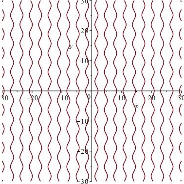
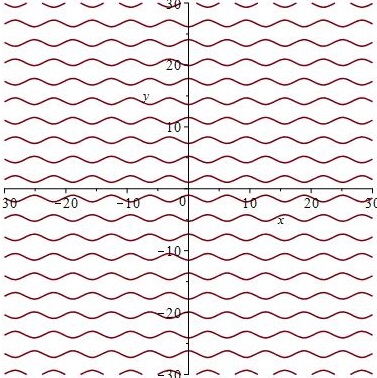
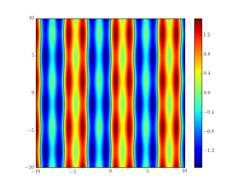
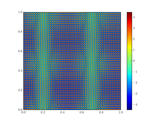
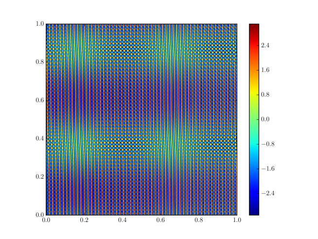
It is possible to realize the Euclidean random field fν0:2:subscript𝑓subscript𝜈0superscript2f_{\nu_{0}}:\mathbb{R}^{2}\rightarrow\mathbb{R} as a trigonometric polynomial (for more details, see (6.3) or (6.4)), with only 444 nonzero coefficients (see the 111st proof of Lemma 6.1 below); a typical sample of the corresponding nodal pictures are shown in Figure 2 (cf. § 6.2.) We may deduce that a.s. 𝒩(fν0;)0𝒩subscript𝑓subscript𝜈00\mathcal{N}(f_{\nu_{0}};\cdot)\equiv 0, i.e. there are no compact domains of fν0subscript𝑓subscript𝜈0f_{\nu_{0}} at all and all the domains are either predominantly horizontal or predominantly vertical, occurring with probability 1212\frac{1}{2}. The analogous situation on the torus occurs for n=m2𝑛superscript𝑚2n=m^{2} with

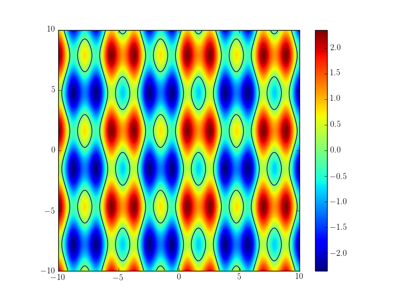
g0;m(x)=12(a1cos(mx1+η1)+a2cos(mx2+η2)),subscript𝑔0𝑚𝑥12subscript𝑎1𝑚subscript𝑥1subscript𝜂1subscript𝑎2𝑚subscript𝑥2subscript𝜂2g_{0;m}(x)=\frac{1}{\sqrt{2}}\cdot\left(a_{1}\cdot\cos(m\cdot x_{1}+\eta_{1})+a_{2}\cdot\cos(m\cdot x_{2}+\eta_{2})\right),

where a1subscript𝑎1a_{1}, a2subscript𝑎2a_{2} are Rayleigh(1)Rayleigh1\text{Rayleigh}(1) distributed independent random variables, and η1,η2[0,2π)subscript𝜂1subscript𝜂202𝜋\eta_{1},\eta_{2}\in[0,2\pi) are random phases uniformly drawn in [0,2π)02𝜋[0,2\pi); in this case the nodal components in Figure 2 all become periodic with nontrivial homology, and their number is of order of magnitude

(2.2) 𝒩(g0)mn.𝒩subscript𝑔0𝑚𝑛\mathcal{N}(g_{0})\approx m\approx\sqrt{n}.

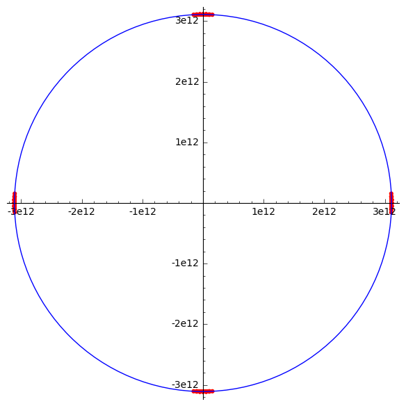
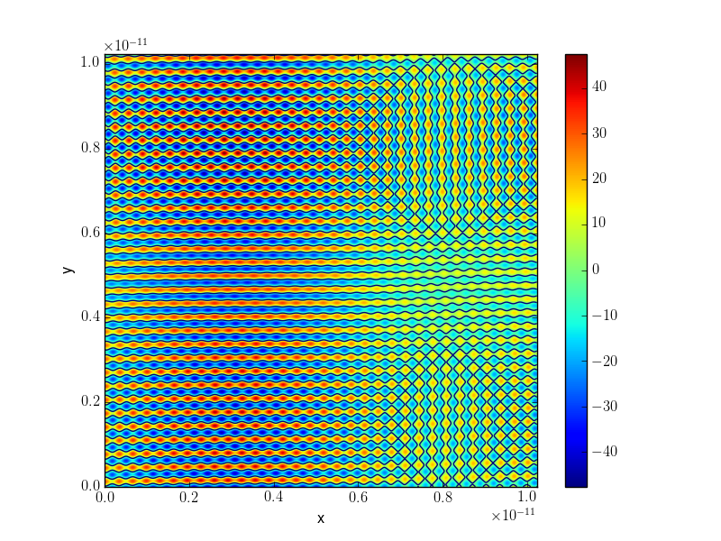
Since the Nazarov-Sodin constant does not vanish outside of the (tilted) Cilleruelo measure, for every finite instance fnsubscript𝑓𝑛f_{n} with nS𝑛𝑆n\in S one would expect for more domains as compared to (2.2), whether or not n𝑛n is a square, i.e., 𝒩(fn)nmuch-greater-than𝒩subscript𝑓𝑛𝑛\mathcal{N}(f_{n})\gg\sqrt{n}. The above intuition has some reservations. A fragment of a sample nodal portrait of fnsubscript𝑓𝑛f_{n} with n𝑛n corresponding to a measure μnsubscript𝜇𝑛\mu_{n} close to Cilleruelo is given in Figure 1.
Refer to caption
Refer to caption
Figure 1. Left: Plot of a fragment of a random “Cilleruello” type eigenfunction, nodal curves in black. Right: corresponding spectral measure. Here n=9676418088513347624474653𝑛9676418088513347624474653n=9676418088513347624474653 and r2(n)=|{(x,y)2:x2+y2=n}|=256subscript𝑟2𝑛conditional-set𝑥𝑦superscript2superscript𝑥2superscript𝑦2𝑛256r_{2}(n)=|\{(x,y)\in\mathbb{Z}^{2}:x^{2}+y^{2}=n\}|=256; for this particular choice of n𝑛n, the corresponding lattice points, shown in red, are concentrated around 444 antipodal points.

It exhibits that, just as in Figure 2, the nodal domains are all predominantly horizontal or vertical, but the suggested effect of the perturbed Cilleruelo shows that the periodic trajectories sometime connect in some percolation-like process, and transform from horizontal to vertical and back. Judging from the small presented fragment it seems difficult to determine to what extent this procedure decreases the total number of nodal domains, in particular whether the expectation is bounded or not. For a higher resolution picture, as well as some further examples of Cilluello eigenfunctions, see Appendix A.

In any case it is likely that the genuine asymptotic behaviour of 𝔼[𝒩(fnj)]𝔼delimited-[]𝒩subscript𝑓subscript𝑛𝑗\mathbb{E}[\mathcal{N}(f_{n_{j}})] depends on the rate of convergence (2.1), hence does not admit a simple asymptotic law. With all our reservations, the above discussion is our basis for the following question.

Question 2.2.

Is it true that for an arbitrary Cilleruelo sequence,

lim infj𝔼[N(fnj)],subscriptlimit-infimum𝑗𝔼delimited-[]𝑁subscript𝑓subscript𝑛𝑗\liminf\limits_{j\rightarrow\infty}\mathbb{E}[N(f_{n_{j}})]\rightarrow\infty,

or, even stronger

𝔼[N(fnj)]nj?much-greater-than𝔼delimited-[]𝑁subscript𝑓subscript𝑛𝑗subscript𝑛𝑗?\mathbb{E}[N(f_{n_{j}})]\gg\sqrt{n_{j}}?

If, as we tend to think, the answer to the latter question is “yes”, then a simple compactness argument yields that for the full sequence nS𝑛𝑆n\in S we have

limn𝔼[𝒩(fn)]=.subscript𝑛𝔼delimited-[]𝒩subscript𝑓𝑛\lim\limits_{n\rightarrow\infty}\mathbb{E}[\mathcal{N}(f_{n})]=\infty.

2.4. The true nature of the Nazarov-Sodin constant

Motivated by the fact that various local quantities, such as the nodal length variance  [KKW], or the expected number of “flips” (see (3.6)) or critical points, only depends on the first non-trivial Fourier coefficient of the measure, we raise the following question.

Question 2.3.

Is it true that cNS(μ)subscript𝑐𝑁𝑆𝜇c_{NS}(\mu) with μ𝒫symm𝜇subscript𝒫symm\mu\in\mathcal{P}_{\text{symm}} only depends on finitely many Fourier coefficients, e.g. μ^(4)^𝜇4\widehat{\mu}(4) or (μ^(4),μ^(8))^𝜇4^𝜇8(\widehat{\mu}(4),\widehat{\mu}(8))?

2.5. Key ideas of the proof of Theorem 1.3

To prove the continuity of cNSsubscript𝑐𝑁𝑆c_{NS} in Theorem 1.3 we wish to show that |cNS(ρ)cNS(ρ)|subscript𝑐𝑁𝑆𝜌subscript𝑐𝑁𝑆superscript𝜌|c_{NS}(\rho)-c_{NS}(\rho^{\prime})| is small for two “close” spectral measures ρ,ρ𝜌superscript𝜌\rho,\rho^{\prime}. To this end we show that for a large R𝑅R there exists a coupling between the random fields fρsubscript𝑓𝜌f_{\rho} and fρsubscript𝑓superscript𝜌f_{\rho^{\prime}}, and that 𝒩(fρ,R)𝒩subscript𝑓𝜌𝑅\mathcal{N}(f_{\rho},R) and 𝒩(fρ,R)𝒩subscript𝑓superscript𝜌𝑅\mathcal{N}(f_{\rho^{\prime}},R) are very likely to be close (in fact, that fρsubscript𝑓𝜌f_{\rho} and fρsubscript𝑓superscript𝜌f_{\rho^{\prime}} are C1superscript𝐶1C^{1}-close and that they have essentially the same nodal components). Of key importance is that both fρsubscript𝑓𝜌f_{\rho} and fρsubscript𝑓superscript𝜌f_{\rho^{\prime}} are not only C1superscript𝐶1C^{1}-close, but also likely to be “stable” in the sense that small perturbations do not change the number of nodal components, except near the boundary. However, we can only prove stability, and the desired properties of the coupling, for square domains 𝒟Rsubscript𝒟𝑅\mathcal{D}_{R} for R𝑅R fixed, and it is thus essential to have bounds on the difference

𝒩(fρ,R)/(4R2)cNS(ρ)𝒩subscript𝑓𝜌𝑅4superscript𝑅2subscript𝑐𝑁𝑆𝜌\mathcal{N}(f_{\rho},R)/(4R^{2})-c_{NS}(\rho)

that are uniform in both ρ𝜌\rho and R𝑅R.

To obtain uniformity in R𝑅R we tile a “huge” square with a fixed “large” square, and count nodal domains entirely contained in the fixed large square. By translation invariance, the expectation over all large squares is the same, hence the scaled number of components in the large square (i.e., scaling by dividing by the area of the square) is the same as the scaled number of components of the huge square, up to an error involving the (scaled) number of nodal components that intersect a boundaries of at least one large square. This in turn can be uniformly bounded (in terms of ρ𝜌\rho) by using Kac-Rice type techniques to uniformly bound the expected number of zeros of fρsubscript𝑓𝜌f_{\rho} lying on a curve (the bound of course depends on its length), cf. Lemma 3.2.

In case the huge square cannot exactly be tiled by large squares, we make use of the following observation: the number of nodal domains entirely contained in some region is bounded from above by the number of “flip points”, i.e., points x=(x1,x2)𝑥subscript𝑥1subscript𝑥2x=(x_{1},x_{2}) where f=fx1=0𝑓𝑓subscript𝑥10f=\frac{\partial f}{\partial x_{1}}=0, and the expected number of such points is, up to a uniform constant, bounded by the area of the region. To show this we again use a Kac-Rice type “local” estimates, cf. Lemma 3.4 and its proof.

Nazarov and Sodin assume that the support of ρ𝜌\rho is not contained in a line, in order for non-degeneracy of (fρ,fρ)subscript𝑓𝜌subscript𝑓𝜌(f_{\rho},\nabla f_{\rho}) to hold. Now, if ρiρsubscript𝜌𝑖𝜌\rho_{i}\Rightarrow\rho and the limiting measure ρ𝜌\rho is non-degenerate, there exists ϵ>0italic-ϵ0\epsilon>0 such that ρ𝜌\rho is outside a small neighbourhood 𝒫ϵsubscript𝒫italic-ϵ\mathcal{P}_{\epsilon} of the degenerate measures within 𝒫𝒫\mathcal{P} defined in § 3 below (see 3.5). The outlined approach above yields continuity of cNSsubscript𝑐𝑁𝑆c_{NS} around ρ𝜌\rho in the complement 𝒫𝒫ϵ𝒫subscript𝒫italic-ϵ\mathcal{P}\setminus\mathcal{P}_{\epsilon}.

On the other hand, if the limit ρ𝜌\rho is degenerate we use a separate argument. First we show that cNS(ρ)=0subscript𝑐𝑁𝑆𝜌0c_{NS}(\rho)=0 by showing that fρsubscript𝑓𝜌f_{\rho}, almost surely, has no bounded nodal domains; similarly this shows that we may assume that all ρisubscript𝜌𝑖\rho_{i} gives rise to non-degenerate fields. As non-degeneracy holds along the full sequence, we can then use Kac-Rice type local argument giving that 𝔼(𝒩(fρi;R))/R20𝔼𝒩subscript𝑓subscript𝜌𝑖𝑅superscript𝑅20\mathbb{E}(\mathcal{N}(f_{\rho_{i}};R))/R^{2}\to 0 as i𝑖i\to\infty.

3. Kac-Rice premise

We begin with collecting some notational conventions. Given a smooth function f𝑓f on 2superscript2\mathbb{R}^{2} let f1=1f=fx1subscript𝑓1subscript1𝑓𝑓subscript𝑥1f_{1}=\partial_{1}f=\frac{\partial f}{\partial x_{1}}, f2=fx2subscript𝑓2𝑓subscript𝑥2f_{2}=\frac{\partial f}{\partial x_{2}}, and f12=12f=2fx1x2subscript𝑓12subscript1subscript2𝑓superscript2𝑓subscript𝑥1subscript𝑥2f_{12}=\partial_{1}\partial_{2}f=\frac{\partial^{2}f}{\partial x_{1}\partial x_{2}} (etc), where x=(x1,x2)2𝑥subscript𝑥1subscript𝑥2superscript2x=(x_{1},x_{2})\in\mathbb{R}^{2}; and similarly for smooth functions f:𝕋2:𝑓superscript𝕋2f:\mathbb{T}^{2}\to\mathbb{R}.

The Kac-Rice formula is a standard tool for computing moments of various local properties of random (Gaussian) fields, such as, for example, number of nodal intersections against a reference curve, number of critical points etc. For our purposes we will not require any result beyond the expectation of the number of zeros 𝒵Fsubscript𝒵𝐹\mathcal{Z}_{F} of a stationary Gaussian field F:𝒟n:𝐹𝒟superscript𝑛F:\mathcal{D}\rightarrow\mathbb{R}^{n} on a compact domain 𝒟n𝒟superscript𝑛\mathcal{D}\subseteq\mathbb{R}^{n} (closed interval for n=1𝑛1n=1), with the sole intention of applying it in the 2d2𝑑2d case. For x𝒟𝑥𝒟x\in\mathcal{D} define the zero density as the conditional Gaussian expectation

(3.1) K1(x)=K1;F(x)=ϕF(x)(0)𝔼[|detJF(x)||F(x)=0],subscript𝐾1𝑥subscript𝐾1𝐹𝑥subscriptitalic-ϕ𝐹𝑥0𝔼delimited-[]conditionalsubscript𝐽𝐹𝑥𝐹𝑥0K_{1}(x)=K_{1;F}(x)=\phi_{F(x)}(0)\cdot\mathbb{E}[|\det{J_{F}(x)}|\big{|}F(x)=0],

where ϕF(x)subscriptitalic-ϕ𝐹𝑥\phi_{F(x)} is the probability density function of the Gaussian vector F(x)n𝐹𝑥superscript𝑛F(x)\in\mathbb{R}^{n}, and JF(x)subscript𝐽𝐹𝑥J_{F}(x) is the Jacobian matrix of F𝐹F at x𝑥x. The Kac-Rice meta-theorem states that, under some non-degeneracy conditions on F𝐹F,

(3.2) 𝔼[𝒵F]=𝒟K1(x)𝑑x;𝔼delimited-[]subscript𝒵𝐹subscript𝒟subscript𝐾1𝑥differential-d𝑥\mathbb{E}[\mathcal{Z}_{F}]=\int\limits_{\mathcal{D}}K_{1}(x)dx;

to our best knowledge the mildest sufficient conditions for the validity of (3.2), due to Azais-Wschebor  [AW, Theorem 6.3], is that for all x𝒟𝑥𝒟x\in\mathcal{D} the distribution of the Gaussian vector F(x)n𝐹𝑥superscript𝑛F(x)\in\mathbb{R}^{n} is non-degenerate.

As for the zero density K1(x)subscript𝐾1𝑥K_{1}(x) in (3.1), since (3.1) is a Gaussian expectation depending on the law of (F(x),JF(x))𝐹𝑥subscript𝐽𝐹𝑥(F(x),J_{F}(x)), it is in principle possible to express K1subscript𝐾1K_{1} in terms of the covariance of F𝐹F. For F𝐹F a derived field of fρsubscript𝑓𝜌f_{\rho} (if, for example, F𝐹F is a restriction of fρsubscript𝑓𝜌f_{\rho} on the reference curve 𝒞𝒞\mathcal{C} in Lemma 3.2 below, or F=(fρ,1fρ)𝐹subscript𝑓𝜌subscript1subscript𝑓𝜌F=(f_{\rho},\partial_{1}f_{\rho}) in Lemma 3.4 below) it is possible to express K1(x)subscript𝐾1𝑥K_{1}(x) in terms of the covariance function

rρ(x,y)=𝔼[fρ(x)fρ(y)]subscript𝑟𝜌𝑥𝑦𝔼delimited-[]subscript𝑓𝜌𝑥subscript𝑓𝜌𝑦r_{\rho}(x,y)=\mathbb{E}[f_{\rho}(x)\cdot f_{\rho}(y)]

and its various derivatives, or, what is equivalent, its spectral measure ρ𝜌\rho, supported on B(1)𝐵1B(1):

(3.3) rρ(x)=B(1)e(x,y)𝑑ρ(y),subscript𝑟𝜌𝑥subscript𝐵1𝑒𝑥𝑦differential-d𝜌𝑦r_{\rho}(x)=\int\limits_{B(1)}e(\langle x,y\rangle)d\rho(y),

where

e(t)=e2πit.𝑒𝑡superscript𝑒2𝜋𝑖𝑡e(t)=e^{2\pi it}.

In case F𝐹F is stationary (see Lemma 3.4 below), K1;F(x)subscript𝐾1𝐹𝑥K_{1;F}(x) in (3.1) is independent of x𝑥x; in this case to prove a uniform upper bound we only need to control it in terms of F𝐹F.

For the Kac-Rice method to apply it is essential that the field is nondegenerate. In order to analyze certain degenerate limit measures we introduce the following notation. Given a stationary Gaussian field fρsubscript𝑓𝜌f_{\rho} with spectral measure ρ𝜌\rho, let C(ρ)𝐶𝜌C(\rho) denote the positive semi-definite covariance matrix

(3.4) C(ρ):=(Var(1fρ(0))Cov(1fρ(0),2fρ(0))Cov(1fρ(0),2fρ(0))Var(2fρ(0))),assign𝐶𝜌matrixVarsubscript1subscript𝑓𝜌0Covsubscript1subscript𝑓𝜌0subscript2subscript𝑓𝜌0Covsubscript1subscript𝑓𝜌0subscript2subscript𝑓𝜌0Varsubscript2subscript𝑓𝜌0C(\rho):=\begin{pmatrix}\operatorname{Var}(\partial_{1}f_{\rho}(0))&\operatorname{Cov}(\partial_{1}f_{\rho}(0),\partial_{2}f_{\rho}(0))\\ \operatorname{Cov}(\partial_{1}f_{\rho}(0),\partial_{2}f_{\rho}(0))&\operatorname{Var}(\partial_{2}f_{\rho}(0))\\ \end{pmatrix},

and let λ(ρ)0𝜆𝜌0\lambda(\rho)\geq 0 denote the smallest eigenvalue of C(ρ)𝐶𝜌C(\rho). As the map ρC(ρ)𝜌𝐶𝜌\rho\to C(\rho) is continuous, the same holds for ρλ(ρ)𝜌𝜆𝜌\rho\to\lambda(\rho). Thus, if we are given ϵ>0italic-ϵ0\epsilon>0 define

(3.5) 𝒫ϵ:={ρ𝒫:λ(ρ)<ϵ}assignsubscript𝒫italic-ϵconditional-set𝜌𝒫𝜆𝜌italic-ϵ\mathcal{P}_{\epsilon}:=\{\rho\in\mathcal{P}:\lambda(\rho)<\epsilon\}

we find that 𝒫𝒫ϵ𝒫subscript𝒫italic-ϵ\mathcal{P}\setminus\mathcal{P}_{\epsilon} is a closed subset of 𝒫𝒫\mathcal{P}. Abusing notation slightly it is convenient to let

𝒫0:={ρ𝒫:λ(ρ)=0}assignsubscript𝒫0conditional-set𝜌𝒫𝜆𝜌0\mathcal{P}_{0}:=\{\rho\in\mathcal{P}:\lambda(\rho)=0\}

denote the set spectral measures giving rise to degenerate fields. (We may interpret the covariance matrix C(ρ)𝐶𝜌C(\rho) as a matrix representing a positive semi-definite quadratic form; non-degenaracy is then equivalent to the form being positive definite. As quadratic forms in two variables can be diagonalised by a rotation, degeneracy implies that after a change of coordinates by rotation, we have Var(1f)=ξ12𝑑ρ(ξ)=0Varsubscript1𝑓superscriptsubscript𝜉12differential-d𝜌𝜉0\operatorname{Var}(\partial_{1}f)=\int\xi_{1}^{2}\,d\rho(\xi)=0, and hence the support of ρ𝜌\rho must be contained in the line ξ1=0subscript𝜉10\xi_{1}=0.)

As we intend to apply the Kac-Rice formula on fρsubscript𝑓𝜌f_{\rho}, for ρ𝒫𝒫ϵ𝜌𝒫subscript𝒫italic-ϵ\rho\in\mathcal{P}\setminus\mathcal{P}_{\epsilon} for some ϵ>0italic-ϵ0\epsilon>0, and some derived random fields (see lemmas 3.2 and 3.4 below) we will need to collect the following facts.

Lemma 3.1.
  1. (1)

    For every unit variance random field F:𝒟:𝐹𝒟F:\mathcal{D}\rightarrow\mathbb{R}, and x𝒟𝑥𝒟x\in\mathcal{D}, the value F(x)𝐹𝑥F(x) is independent of the gradient F(x)𝐹𝑥\nabla F(x).

  2. (2)

    The variances Var(1fρ),Var(2fρ)Varsubscript1subscript𝑓𝜌Varsubscript2subscript𝑓𝜌\operatorname{Var}(\partial_{1}f_{\rho}),\operatorname{Var}(\partial_{2}f_{\rho}) of the first partial derivatives is bounded away from 00, uniformly for ρ𝒫𝒫ϵ𝜌𝒫subscript𝒫italic-ϵ\rho\in\mathcal{P}\setminus\mathcal{P}_{\epsilon}.

The proof of Lemma 3.1 will be given in § 3.4.

3.1. Intersections with curves and flips

We begin with a bound on expected number of nodal intersections with curves, whose proof will be given in § 3.4.

Lemma 3.2.

Let 𝒞2𝒞superscript2\mathcal{C}\subseteq\mathbb{R}^{2} be a smooth curve of length \mathcal{L}, and 𝒩(fρ,𝒞)𝒩subscript𝑓𝜌𝒞\mathcal{N}(f_{\rho},\mathcal{C}) the number of nodal intersections of fρsubscript𝑓𝜌f_{\rho} with 𝒞𝒞\mathcal{C}, ρ𝒫𝜌𝒫\rho\in\mathcal{P}. Then

𝔼[𝒩(fρ,𝒞)]=O()𝔼delimited-[]𝒩subscript𝑓𝜌𝒞𝑂\mathbb{E}[\mathcal{N}(f_{\rho},\mathcal{C})]=O(\mathcal{L})

with constant involved in the ‘O𝑂O’-notation absolute.

The notion of “nodal flips” will be very useful for giving uniform upper bounds on the number of nodal domains.

Notation 3.3.

For 𝒟2𝒟superscript2\mathcal{D}\subseteq\mathbb{R}^{2} a nice closed domain we denote the number of vertical and horizontal nodal flips

(3.6) S1(fρ;𝒟)=#{x𝒟:fρ(x)=1fρ(x)=0},S2(fρ;𝒟)=#{x𝒟:fρ(x)=2fρ(x)=0},formulae-sequencesubscript𝑆1subscript𝑓𝜌𝒟#conditional-set𝑥𝒟subscript𝑓𝜌𝑥subscript1subscript𝑓𝜌𝑥0subscript𝑆2subscript𝑓𝜌𝒟#conditional-set𝑥𝒟subscript𝑓𝜌𝑥subscript2subscript𝑓𝜌𝑥0\begin{split}S_{1}(f_{\rho};\mathcal{D})&=\#\{x\in\mathcal{D}:\>f_{\rho}(x)=\partial_{1}f_{\rho}(x)=0\},\\ S_{2}(f_{\rho};\mathcal{D})&=\#\{x\in\mathcal{D}:\>f_{\rho}(x)=\partial_{2}f_{\rho}(x)=0\},\end{split}

respectively.

Lemma 3.4.

For all ρ𝒫𝒫0𝜌𝒫subscript𝒫0\rho\in\mathcal{P}\setminus\mathcal{P}_{0}, we have

(3.7) 𝔼[S1(fρ;𝒟)]=O(Area(𝒟)Var(2fρ)1/2),𝔼[S2(fρ;𝒟)]=(Area(𝒟)Var(1fρ)1/2),\begin{split}\mathbb{E}[S_{1}(f_{\rho};\mathcal{D})]&=O\left(\operatorname{Area}(\mathcal{D})\cdot\operatorname{Var}(\partial_{2}f_{\rho})^{1/2}\right),\\ \mathbb{E}[S_{2}(f_{\rho};\mathcal{D})]&=\left(\operatorname{Area}(\mathcal{D})\cdot\operatorname{Var}(\partial_{1}f_{\rho})^{1/2}\right),\end{split}

and consequently

max(𝔼[S1(fρ;𝒟)],𝔼[S2(fρ;𝒟)])=O(Area(𝒟))𝔼delimited-[]subscript𝑆1subscript𝑓𝜌𝒟𝔼delimited-[]subscript𝑆2subscript𝑓𝜌𝒟𝑂Area𝒟\max(\mathbb{E}[S_{1}(f_{\rho};\mathcal{D})],\mathbb{E}[S_{2}(f_{\rho};\mathcal{D})])=O(\operatorname{Area}(\mathcal{D}))

with constants involved in the ‘O𝑂O’-notation absolute.

Lemma 3.4 will be proved in § 3.4. As it was mentioned above, for ρ𝒫ϵ𝜌subscript𝒫italic-ϵ\rho\in\mathcal{P}_{\epsilon} we may arrange that, after rotating if necessary, either Var(1fρ)Varsubscript1subscript𝑓𝜌\operatorname{Var}(\partial_{1}f_{\rho}) or Var(2fρ)Varsubscript2subscript𝑓𝜌\operatorname{Var}(\partial_{2}f_{\rho}) is at most ϵitalic-ϵ\epsilon. To treat the degenerate case ρ𝒫0𝜌subscript𝒫0\rho\in\mathcal{P}_{0} we record the following fact.

Lemma 3.5.

If ρ𝒫0𝜌subscript𝒫0\rho\in\mathcal{P}_{0} then 𝒩(fρ;)0𝒩subscript𝑓𝜌0\mathcal{N}(f_{\rho};\cdot)\equiv 0. In particular in this case (1.4) holds with cNS(ρ)=0subscript𝑐𝑁𝑆𝜌0c_{NS}(\rho)=0.

Proof.

After changing coordinates by a rotation, we may assume that Var(1f)=0Varsubscript1𝑓0\operatorname{Var}(\partial_{1}f)=0. Hence, almost surely, we have f(x1,x2)=g(x2)𝑓subscript𝑥1subscript𝑥2𝑔subscript𝑥2f(x_{1},x_{2})=g(x_{2}) for some function g𝑔g, and thus f𝑓f has no compact nodal domains, and in particular cNS(ρ)=0subscript𝑐𝑁𝑆𝜌0c_{NS}(\rho)=0. ∎

3.2. Proof of Proposition 1.1

Proof.

First, we may assume that ρ𝒫𝒫0𝜌𝒫subscript𝒫0\rho\in\mathcal{P}\setminus\mathcal{P}_{0} by the virtue of Lemma 3.5, so that we are eligible to apply Lemma 3.4 on fρsubscript𝑓𝜌f_{\rho}. Now let R2R10very-much-greater-thansubscript𝑅2subscript𝑅1very-much-greater-than0R_{2}\ggg R_{1}\ggg 0 be a two big real numbers; for notational convenience we will at first assume that

(3.8) R2=kR1subscript𝑅2𝑘subscript𝑅1R_{2}=kR_{1}

is an integer multiple of R2subscript𝑅2R_{2}, k1much-greater-than𝑘1k\gg 1. We divide the square 𝒟R2=[R2,R2]2subscript𝒟subscript𝑅2superscriptsubscript𝑅2subscript𝑅22\mathcal{D}_{R_{2}}=[-R_{2},R_{2}]^{2} into 4k2=4R22R124superscript𝑘24superscriptsubscript𝑅22superscriptsubscript𝑅124k^{2}=4\frac{R_{2}^{2}}{R_{1}^{2}} smaller squares

{𝒟R2;i,j}i,j=12ksubscriptsubscript𝒟subscript𝑅2𝑖𝑗𝑖𝑗12𝑘\{\mathcal{D}_{R_{2};i,j}\}_{i,j=1\ldots 2k}

of side length R1subscript𝑅1R_{1}, disjoint save to boundary overlaps. Every nodal component lying in 𝒟R2subscript𝒟subscript𝑅2\mathcal{D}_{R_{2}} is either lying entirely in one of the 𝒟R2;i,jsubscript𝒟subscript𝑅2𝑖𝑗\mathcal{D}_{R_{2};i,j} or intersects at least one of the vertical or horizontal line segments, {x=iT,|y|R2}formulae-sequence𝑥𝑖𝑇𝑦subscript𝑅2\{x=i\cdot T,\,|y|\leq R_{2}\}, i=k,k𝑖𝑘𝑘i=-k,\ldots k, or {y=jT,|x|R2}formulae-sequence𝑦𝑗𝑇𝑥subscript𝑅2\{y=j\cdot T,\,|x|\leq R_{2}\}, j=k,,k𝑗𝑘𝑘j=-k,\ldots,k respectively. Let 𝒩(fρ;𝒟R2;i,j)𝒩subscript𝑓𝜌subscript𝒟subscript𝑅2𝑖𝑗\mathcal{N}(f_{\rho};\mathcal{D}_{R_{2};i,j}) be the number of nodal components of fρsubscript𝑓𝜌f_{\rho} lying in 𝒟R2;i,jsubscript𝒟subscript𝑅2𝑖𝑗\mathcal{D}_{R_{2};i,j}, and 𝒵(fρ;R2,x=iR1)𝒵subscript𝑓𝜌subscript𝑅2𝑥𝑖subscript𝑅1\mathcal{Z}(f_{\rho};R_{2},x=iR_{1}), 𝒵(fρ;R2,y=jR1)𝒵subscript𝑓𝜌subscript𝑅2𝑦𝑗subscript𝑅1\mathcal{Z}(f_{\rho};R_{2},y=jR_{1}) be the number of nodal intersections of fρsubscript𝑓𝜌f_{\rho} against a finite vertical or horizontal line segment as above.

The above approach shows that

(3.9) 𝒩(fρ;R2)=1i,j2k𝒩(fρ;𝒟R2;i,j)+O(i=kk𝒵(fρ;R2,x=iR1))+O(j=kk𝒵(fρ;R2,y=jR1)).𝒩subscript𝑓𝜌subscript𝑅2subscriptformulae-sequence1𝑖𝑗2𝑘𝒩subscript𝑓𝜌subscript𝒟subscript𝑅2𝑖𝑗𝑂superscriptsubscript𝑖𝑘𝑘𝒵subscript𝑓𝜌subscript𝑅2𝑥𝑖subscript𝑅1𝑂superscriptsubscript𝑗𝑘𝑘𝒵subscript𝑓𝜌subscript𝑅2𝑦𝑗subscript𝑅1\begin{split}\mathcal{N}(f_{\rho};R_{2})&=\sum\limits_{1\leq i,j\leq 2k}\mathcal{N}(f_{\rho};\mathcal{D}_{R_{2};i,j})+O\left(\sum\limits_{i=-k}^{k}\mathcal{Z}(f_{\rho};R_{2},x=iR_{1})\right)\\ &+O\left(\sum\limits_{j=-k}^{k}\mathcal{Z}(f_{\rho};R_{2},y=jR_{1})\right).\end{split}

We now take expectation of both sides of (3.9); using the translation invariance of fρsubscript𝑓𝜌f_{\rho}, and Lemma 3.2 we find that

(3.10) 𝔼[𝒩(fρ;R2)]=4k2𝔼[𝒩(fρ;R1/2)]+O(kR2),𝔼delimited-[]𝒩subscript𝑓𝜌subscript𝑅24superscript𝑘2𝔼delimited-[]𝒩subscript𝑓𝜌subscript𝑅12𝑂𝑘subscript𝑅2\mathbb{E}[\mathcal{N}(f_{\rho};R_{2})]=4k^{2}\cdot\mathbb{E}[\mathcal{N}(f_{\rho};R_{1}/2)]+O(kR_{2}),

where the constant involved in the ‘O𝑂O’-notation is absolute. A simple manipulation with (3.10), bearing in mind (3.8), now implies

(3.11) |𝔼[𝒩(fρ;R2)]4R22𝔼[𝒩(fρ;R1/2)]R12|=O(1R1)𝔼delimited-[]𝒩subscript𝑓𝜌subscript𝑅24superscriptsubscript𝑅22𝔼delimited-[]𝒩subscript𝑓𝜌subscript𝑅12superscriptsubscript𝑅12𝑂1subscript𝑅1\left|\frac{\mathbb{E}[\mathcal{N}(f_{\rho};R_{2})]}{4R_{2}^{2}}-\frac{\mathbb{E}[\mathcal{N}(f_{\rho};R_{1}/2)]}{R_{1}^{2}}\right|=O\left(\frac{1}{R_{1}}\right)

with the constant involved in the ‘O𝑂O’-notation absolute, with (3.11).

In case R2subscript𝑅2R_{2} is not an integer multiple of R1subscript𝑅1R_{1}, in the above argument we leave a small rectangular corridor of size at most R1×R2subscript𝑅1subscript𝑅2R_{1}\times R_{2} (in fact, two such corridors). In this case the estimate (3.11) should be replaced by

(3.12) |𝔼[𝒩(fρ;R2)]4R22𝔼[𝒩(fρ;R1/2)]R12|=O(1R1+R1R2),𝔼delimited-[]𝒩subscript𝑓𝜌subscript𝑅24superscriptsubscript𝑅22𝔼delimited-[]𝒩subscript𝑓𝜌subscript𝑅12superscriptsubscript𝑅12𝑂1subscript𝑅1subscript𝑅1subscript𝑅2\left|\frac{\mathbb{E}[\mathcal{N}(f_{\rho};R_{2})]}{4R_{2}^{2}}-\frac{\mathbb{E}[\mathcal{N}(f_{\rho};R_{1}/2)]}{R_{1}^{2}}\right|=O\left(\frac{1}{R_{1}}+\frac{R_{1}}{R_{2}}\right),

with O(R1R2)𝑂subscript𝑅1subscript𝑅2O(\frac{R_{1}}{R_{2}}) coming from the contribution of the small rectangular leftover corridor thinking of R2subscript𝑅2R_{2} much bigger than R1subscript𝑅1R_{1}; here we used Lemma 3.4, valid since we assumed ρ𝒫𝒫0𝜌𝒫subscript𝒫0\rho\in\mathcal{P}\setminus\mathcal{P}_{0}. The latter estimate (3.12) shows that {𝔼[𝒩(fρ;R)]4R2}𝔼delimited-[]𝒩subscript𝑓𝜌𝑅4superscript𝑅2\left\{\frac{\mathbb{E}[\mathcal{N}(f_{\rho};R)]}{4R^{2}}\right\} satisfies the Cauchy convergence criterion (if R1subscript𝑅1R_{1} and R2subscript𝑅2R_{2} are of comparable size then we use the triangle inequality, after tiling both 𝒟R2subscript𝒟subscript𝑅2\mathcal{D}_{R_{2}} and 𝒟R1/2subscript𝒟subscript𝑅12\mathcal{D}_{R_{1}/2} with much finer mesh size), we then denote its limit by

cNS(ρ):=limR𝔼[𝒩(fρ;R)]4R2.assignsubscript𝑐𝑁𝑆𝜌subscript𝑅𝔼delimited-[]𝒩subscript𝑓𝜌𝑅4superscript𝑅2c_{NS}(\rho):=\lim\limits_{R\rightarrow\infty}\frac{\mathbb{E}[\mathcal{N}(f_{\rho};R)]}{4R^{2}}.

Now that the existence of the limit cNS(ρ)subscript𝑐𝑁𝑆𝜌c_{NS}(\rho) is proved, we may assume that R2subscript𝑅2R_{2} is an integer multiple of R1subscript𝑅1R_{1}, and take the limit R2subscript𝑅2R_{2}\rightarrow\infty in (3.11); it yields

(3.13) |𝔼[𝒩(fρ;R1/2)]R12cNS(ρ)|=O(1R1),𝔼delimited-[]𝒩subscript𝑓𝜌subscript𝑅12superscriptsubscript𝑅12subscript𝑐𝑁𝑆𝜌𝑂1subscript𝑅1\left|\frac{\mathbb{E}[\mathcal{N}(f_{\rho};R_{1}/2)]}{R_{1}^{2}}-c_{NS}(\rho)\right|=O\left(\frac{1}{R_{1}}\right),

again with the constant in the‘O𝑂O’-notation on the r.h.s. absolute. We conclude the proof of Proposition 1.1 by noticing that (3.13) is a restatement of (1.4) (e.g. replace R1subscript𝑅1R_{1} by R/2𝑅2R/2).

3.3. Proof of Proposition 1.2

Proof.

Again, for ρ𝒫0𝜌subscript𝒫0\rho\in\mathcal{P}_{0} there is nothing to prove here thanks to Lemma 3.5, so that from this point on we assume that ρ𝒫𝒫0𝜌𝒫subscript𝒫0\rho\in\mathcal{P}\setminus\mathcal{P}_{0}. Let

(3.14) ξ=ξ(ρ):=lim infR𝔼[|𝒩(fρ;R)4R2cNS(ρ)|];𝜉𝜉𝜌assignsubscriptlimit-infimum𝑅𝔼delimited-[]𝒩subscript𝑓𝜌𝑅4superscript𝑅2subscript𝑐𝑁𝑆𝜌\xi=\xi(\rho):=\liminf\limits_{R\rightarrow\infty}\mathbb{E}\left[\left|\frac{\mathcal{N}(f_{\rho};R)}{4R^{2}}-c_{NS}(\rho)\right|\right];

in what follows we argue that, in fact, ξ𝜉\xi is the limit. Let ϵ>0italic-ϵ0\epsilon>0 be given and R1=R1(ρ,ϵ)>0subscript𝑅1subscript𝑅1𝜌italic-ϵ0R_{1}=R_{1}(\rho,\epsilon)>0 such that

(3.15) 𝔼[|𝒩(fρ;R1/2)R12cNS(ρ)|]<ξ+ϵ.𝔼delimited-[]𝒩subscript𝑓𝜌subscript𝑅12superscriptsubscript𝑅12subscript𝑐𝑁𝑆𝜌𝜉italic-ϵ\mathbb{E}\left[\left|\frac{\mathcal{N}(f_{\rho};R_{1}/2)}{R_{1}^{2}}-c_{NS}(\rho)\right|\right]<\xi+\epsilon.

Following the proof of Proposition 1.1 let R2R10much-greater-thansubscript𝑅2subscript𝑅1much-greater-than0R_{2}\gg R_{1}\gg 0 be a large real number; as before we divide the square 𝒟R2=[R2,R2]2subscript𝒟subscript𝑅2superscriptsubscript𝑅2subscript𝑅22\mathcal{D}_{R_{2}}=[-R_{2},R_{2}]^{2} into the smaller squares {𝒟R2,i,j}1i,j2ksubscriptsubscript𝒟subscript𝑅2𝑖𝑗formulae-sequence1𝑖𝑗2𝑘\{\mathcal{D}_{R_{2},i,j}\}_{1\leq i,j\leq 2k} of side length R1subscript𝑅1R_{1} leaving a couple of corridors of size at most R1×R2subscript𝑅1subscript𝑅2R_{1}\times R_{2}, and write (cf. 3.9)

(3.16) 0𝒩(fρ;R2)1i,j2k𝒩(fρ;𝒟R2;i,j)i=kk𝒵(fρ;R2,x=iR1)+j=kk𝒵(fρ;R2,y=jR1)+𝒩(fρ;R2,R1),0𝒩subscript𝑓𝜌subscript𝑅2subscriptformulae-sequence1𝑖𝑗2𝑘𝒩subscript𝑓𝜌subscript𝒟subscript𝑅2𝑖𝑗superscriptsubscript𝑖𝑘𝑘𝒵subscript𝑓𝜌subscript𝑅2𝑥𝑖subscript𝑅1superscriptsubscript𝑗𝑘𝑘𝒵subscript𝑓𝜌subscript𝑅2𝑦𝑗subscript𝑅1𝒩subscript𝑓𝜌subscriptsubscript𝑅2subscript𝑅1\begin{split}0&\leq\mathcal{N}(f_{\rho};R_{2})-\sum\limits_{1\leq i,j\leq 2k}\mathcal{N}(f_{\rho};\mathcal{D}_{R_{2};i,j})\leq\sum\limits_{i=-k}^{k}\mathcal{Z}(f_{\rho};R_{2},x=iR_{1})\\ &+\sum\limits_{j=-k}^{k}\mathcal{Z}(f_{\rho};R_{2},y=jR_{1})+\mathcal{N}(f_{\rho};\mathcal{F}_{R_{2},R_{1}}),\end{split}

where we denoted R2,R1subscriptsubscript𝑅2subscript𝑅1\mathcal{F}_{R_{2},R_{1}} to be the union of the two leftover rectangular corridors, and 𝒩(fρ,R2,R1)𝒩subscript𝑓𝜌subscriptsubscript𝑅2subscript𝑅1\mathcal{N}(f_{\rho},\mathcal{F}_{R_{2},R_{1}}) the corresponding number of nodal domains lying entirely inside R2,R1subscriptsubscript𝑅2subscript𝑅1\mathcal{F}_{R_{2},R_{1}}.

Taking the expectation of both sides of (3.16) and dividing by 4R224superscriptsubscript𝑅224R_{2}^{2} we have that (using the non-negativity of the l.h.s. of (3.16))

(3.17) 𝔼[|𝒩(fρ;R2)4R2214k21i,j2k𝒩(fρ;𝒟R2;i,j)R12|]=O(1R1+R1R2),𝔼delimited-[]𝒩subscript𝑓𝜌subscript𝑅24superscriptsubscript𝑅2214superscript𝑘2subscriptformulae-sequence1𝑖𝑗2𝑘𝒩subscript𝑓𝜌subscript𝒟subscript𝑅2𝑖𝑗superscriptsubscript𝑅12𝑂1subscript𝑅1subscript𝑅1subscript𝑅2\begin{split}\mathbb{E}\left[\left|\frac{\mathcal{N}(f_{\rho};R_{2})}{4R_{2}^{2}}-\frac{1}{4k^{2}}\cdot\sum\limits_{1\leq i,j\leq 2k}\frac{\mathcal{N}(f_{\rho};\mathcal{D}_{R_{2};i,j})}{R_{1}^{2}}\right|\right]=O\left(\frac{1}{R_{1}}+\frac{R_{1}}{R_{2}}\right),\end{split}

thanks to Lemma 3.4, valid for ρ𝒫𝒫0𝜌𝒫subscript𝒫0\rho\in\mathcal{P}\setminus\mathcal{P}_{0}. On the other hand, by (3.15), the triangle inequality, and the translation invariance of fρsubscript𝑓𝜌f_{\rho}, we have that

(3.18) 𝔼[|14k21i,j2k𝒩(fρ;𝒟R2;i,j)R12cNS(ρ)|]14k21i,j2k𝔼[|𝒩(fρ;𝒟R2;i,j)R12cNS(ρ)|]=𝔼[|𝒩(fρ;R1/2)R12cNS(ρ)|]<ξ+ϵ.𝔼delimited-[]14superscript𝑘2subscriptformulae-sequence1𝑖𝑗2𝑘𝒩subscript𝑓𝜌subscript𝒟subscript𝑅2𝑖𝑗superscriptsubscript𝑅12subscript𝑐𝑁𝑆𝜌14superscript𝑘2subscriptformulae-sequence1𝑖𝑗2𝑘𝔼delimited-[]𝒩subscript𝑓𝜌subscript𝒟subscript𝑅2𝑖𝑗superscriptsubscript𝑅12subscript𝑐𝑁𝑆𝜌𝔼delimited-[]𝒩subscript𝑓𝜌subscript𝑅12superscriptsubscript𝑅12subscript𝑐𝑁𝑆𝜌𝜉italic-ϵ\begin{split}&\mathbb{E}\left[\left|\frac{1}{4k^{2}}\cdot\sum\limits_{1\leq i,j\leq 2k}\frac{\mathcal{N}(f_{\rho};\mathcal{D}_{R_{2};i,j})}{R_{1}^{2}}-c_{NS}(\rho)\right|\right]\\ &\leq\frac{1}{4k^{2}}\sum\limits_{1\leq i,j\leq 2k}\mathbb{E}\left[\left|\frac{\mathcal{N}(f_{\rho};\mathcal{D}_{R_{2};i,j})}{R_{1}^{2}}-c_{NS}(\rho)\right|\right]\\ &=\mathbb{E}\left[\left|\frac{\mathcal{N}(f_{\rho};R_{1}/2)}{R_{1}^{2}}-c_{NS}(\rho)\right|\right]<\xi+\epsilon.\end{split}

We have then

(3.19) 𝔼[|𝒩(fρ;R2)4R22cNS(ρ)|]𝔼[|𝒩(fρ;R2)4R2214k21i,j2k𝒩(fρ;𝒟R2;i,j)R12|]+𝔼[|14k21i,j2k𝒩(fρ;𝒟R2;i,j)R12cNS(ρ)|]<ξ+ϵ+O(1R1+R1R2).𝔼delimited-[]𝒩subscript𝑓𝜌subscript𝑅24superscriptsubscript𝑅22subscript𝑐𝑁𝑆𝜌𝔼delimited-[]𝒩subscript𝑓𝜌subscript𝑅24superscriptsubscript𝑅2214superscript𝑘2subscriptformulae-sequence1𝑖𝑗2𝑘𝒩subscript𝑓𝜌subscript𝒟subscript𝑅2𝑖𝑗superscriptsubscript𝑅12𝔼delimited-[]14superscript𝑘2subscriptformulae-sequence1𝑖𝑗2𝑘𝒩subscript𝑓𝜌subscript𝒟subscript𝑅2𝑖𝑗superscriptsubscript𝑅12subscript𝑐𝑁𝑆𝜌𝜉italic-ϵ𝑂1subscript𝑅1subscript𝑅1subscript𝑅2\begin{split}&\mathbb{E}\left[\left|\frac{\mathcal{N}(f_{\rho};R_{2})}{4R_{2}^{2}}-c_{NS}(\rho)\right|\right]\leq\mathbb{E}\left[\left|\frac{\mathcal{N}(f_{\rho};R_{2})}{4R_{2}^{2}}-\frac{1}{4k^{2}}\cdot\sum\limits_{1\leq i,j\leq 2k}\frac{\mathcal{N}(f_{\rho};\mathcal{D}_{R_{2};i,j})}{R_{1}^{2}}\right|\right]\\ &+\mathbb{E}\left[\left|\frac{1}{4k^{2}}\cdot\sum\limits_{1\leq i,j\leq 2k}\frac{\mathcal{N}(f_{\rho};\mathcal{D}_{R_{2};i,j})}{R_{1}^{2}}-c_{NS}(\rho)\right|\right]<\xi+\epsilon+O\left(\frac{1}{R_{1}}+\frac{R_{1}}{R_{2}}\right).\end{split}

by Lemma 3.4, (3.17), (3.18), and, again, the triangle inequality. Since ϵ>0italic-ϵ0\epsilon>0 on the r.h.s. of (3.19) is arbitrary, fixing R10much-greater-thansubscript𝑅10R_{1}\gg 0 satisfying (3.15) arbitrarily big, and taking lim supR2subscriptlimit-supremumsubscript𝑅2\limsup\limits_{R_{2}\rightarrow\infty} of both sides of (3.19) yields

lim supR𝔼[|𝒩(fρ;R)4R2cNS(ρ)|]ξ;subscriptlimit-supremum𝑅𝔼delimited-[]𝒩subscript𝑓𝜌𝑅4superscript𝑅2subscript𝑐𝑁𝑆𝜌𝜉\limsup\limits_{R\rightarrow\infty}\mathbb{E}\left[\left|\frac{\mathcal{N}(f_{\rho};R)}{4R^{2}}-c_{NS}(\rho)\right|\right]\leq\xi;

comparing the latter equality with (3.14) finally yields the existence of the limit (1.5).

3.4. Proofs of the local estimates

Proof of Lemma 3.1.

Let rF(x,y)=𝔼[F(x)F(y)]subscript𝑟𝐹𝑥𝑦𝔼delimited-[]𝐹𝑥𝐹𝑦r_{F}(x,y)=\mathbb{E}[F(x)\cdot F(y)] be the covariance function of F𝐹F, by the assumptions of Lemma 3.1 we have that

(3.20) 𝔼[f(x)f(x)]=rF(x,x)1.𝔼delimited-[]𝑓𝑥𝑓𝑥subscript𝑟𝐹𝑥𝑥1\mathbb{E}[f(x)\cdot f(x)]=r_{F}(x,x)\equiv 1.

The independence of F(x)𝐹𝑥F(x) and F(x)𝐹𝑥\nabla F(x) then follows upon differentiating (3.20) concluding the first part of Lemma 3.1. The second part of Lemma 3.1 is obvious from the definition (3.4) of C(ρ)𝐶𝜌C(\rho) bearing in mind the aforementioned diagonalisation of C(ρ)𝐶𝜌C(\rho) by a rotation (see the interpretation of C(ρ)𝐶𝜌C(\rho) and 𝒫ϵsubscript𝒫italic-ϵ\mathcal{P}_{\epsilon} immediately after (3.5)).

Proof of Lemma 3.2.

Let γ:[0,]2:𝛾0superscript2\gamma:[0,\mathcal{L}]\rightarrow\mathbb{R}^{2} be an arc-length parametrization of 𝒞𝒞\mathcal{C}, and

g(t)=g𝒞,ρ(t)=fρ(γ(t))𝑔𝑡subscript𝑔𝒞𝜌𝑡subscript𝑓𝜌𝛾𝑡g(t)=g_{\mathcal{C},\rho}(t)=f_{\rho}(\gamma(t))

be the restriction g:[0,]:𝑔0g:[0,\mathcal{L}]\rightarrow\mathbb{R} of fρsubscript𝑓𝜌f_{\rho} along 𝒞𝒞\mathcal{C}. The process g𝑔g is centred Gaussian, with covariance function

(3.21) rg(t1,t2)=rρ(γ(t2)γ(t1))subscript𝑟𝑔subscript𝑡1subscript𝑡2subscript𝑟𝜌𝛾subscript𝑡2𝛾subscript𝑡1r_{g}(t_{1},t_{2})=r_{\rho}(\gamma(t_{2})-\gamma(t_{1}))

with rρsubscript𝑟𝜌r_{\rho} the covariance function of fρsubscript𝑓𝜌f_{\rho}.

The number of nodal intersections of fρsubscript𝑓𝜌f_{\rho} against 𝒞𝒞\mathcal{C} is then a.s. equal to 𝒩(fρ,𝒞)=𝒵g𝒩subscript𝑓𝜌𝒞subscript𝒵𝑔\mathcal{N}(f_{\rho},\mathcal{C})=\mathcal{Z}_{g}, the number of zeros of g𝑔g on [0,]0[0,\mathcal{L}]. Since fρsubscript𝑓𝜌f_{\rho} has unit variance, so does g𝑔g; therefore (Lemma 3.1) for every t[0,]𝑡0t\in[0,\mathcal{L}] the value g(t)𝑔𝑡g(t) is independent of the derivative g(t)superscript𝑔𝑡g^{\prime}(t). We then have by Kac-Rice  [AW, Theorem 6.3]

𝔼[g]=0K1(t)𝑑t,𝔼delimited-[]subscript𝑔superscriptsubscript0subscript𝐾1𝑡differential-d𝑡\mathbb{E}[\mathbb{Z}_{g}]=\int\limits_{0}^{\mathcal{L}}K_{1}(t)dt,

where

K1(t)=K1;g(t)=1π2rgt1t2|t1=t2=tsubscript𝐾1𝑡subscript𝐾1𝑔𝑡1𝜋evaluated-atsuperscript2subscript𝑟𝑔subscript𝑡1subscript𝑡2subscript𝑡1subscript𝑡2𝑡K_{1}(t)=K_{1;g}(t)=\frac{1}{\pi}\sqrt{\frac{\partial^{2}r_{g}}{\partial t_{1}\partial t_{2}}\bigg{|}_{t_{1}=t_{2}=t}}

is the zero density of g𝑔g. The statement of Lemma 3.2 will follow once we show that the mixed second derivative 2rgt1t2superscript2subscript𝑟𝑔subscript𝑡1subscript𝑡2\frac{\partial^{2}r_{g}}{\partial t_{1}\partial t_{2}} of rgsubscript𝑟𝑔r_{g} is uniformly bounded by an absolute constant, independent of γ𝛾\gamma and ρ𝒫𝜌𝒫\rho\in\mathcal{P}.

To this end we differentiate (3.21) to compute

t1t2rg(t1,t2)=γ˙(t1)Hrρ(γ(t2)γ(t1))γ˙(t2)t,subscriptsubscript𝑡1subscriptsubscript𝑡2subscript𝑟𝑔subscript𝑡1subscript𝑡2˙𝛾subscript𝑡1subscript𝐻subscript𝑟𝜌𝛾subscript𝑡2𝛾subscript𝑡1˙𝛾superscriptsubscript𝑡2𝑡\partial_{t_{1}}\partial_{t_{2}}r_{g}(t_{1},t_{2})=-\dot{\gamma}(t_{1})\cdot H_{r_{\rho}}(\gamma(t_{2})-\gamma(t_{1}))\cdot\dot{\gamma}(t_{2})^{t},

where Hrρsubscript𝐻subscript𝑟𝜌H_{r_{\rho}} is the Hessian of rρsubscript𝑟𝜌r_{\rho}. That

t1t2rg(t1,t2)subscriptsubscript𝑡1subscriptsubscript𝑡2subscript𝑟𝑔subscript𝑡1subscript𝑡2\partial_{t_{1}}\partial_{t_{2}}r_{g}(t_{1},t_{2})

is bounded by an absolute constant then follows from the fact that

γ˙(t1)=γ˙(t2)=1,norm˙𝛾subscript𝑡1norm˙𝛾subscript𝑡21\|\dot{\gamma}(t_{1})\|=\|\dot{\gamma}(t_{2})\|=1,

and that Hrρsubscript𝐻subscript𝑟𝜌H_{r_{\rho}} is bounded follows by differentiating (3.3), using the bounded support of ρ𝜌\rho.

Proof of Lemma 3.4.

To prove the first assertion we record the following useful fact about nondegenerate centred Gaussians: with (X,Y,Z)𝑋𝑌𝑍(X,Y,Z) denoting components of a nondegenerate multivariate normal distribution having mean zero, we have

(3.22) Var(X|Y=Z=0)Var(X).Varconditional𝑋𝑌𝑍0Var𝑋\operatorname{Var}(X|Y=Z=0)\leq\operatorname{Var}(X).

While it is easy to validate (3.22) by an explicit computation, it is also a (very) particular consequence of the vastly general Gaussian Correlation Inequality  [Roy].

Now, by Kac-Rice  [AW, Theorem 6.3] it follows that, if for all x𝒟𝑥𝒟x\in\mathcal{D}, the Gaussian distribution of

(3.23) F(x):=(fρ(x),1fρ(x))assign𝐹𝑥subscript𝑓𝜌𝑥subscript1subscript𝑓𝜌𝑥F(x):=(f_{\rho}(x),\partial_{1}f_{\rho}(x))

is non-degenerate (holding by both parts of Lemma 3.1), then (3.2) is satisfied with

K1(x)=K1;ρ(x)subscript𝐾1𝑥subscript𝐾1𝜌𝑥K_{1}(x)=K_{1;\rho}(x)

the appropriately defined flips density (3.1) with F𝐹F given by (3.23), and by stationarity we have

(3.24) K1(x)K1(0).subscript𝐾1𝑥subscript𝐾10K_{1}(x)\equiv K_{1}(0).

Now from (3.24) and (3.2) it then follows that

(3.25) 𝔼[S1(fρ;𝒟)]=K1(0)Area(𝒟),𝔼delimited-[]subscript𝑆1subscript𝑓𝜌𝒟subscript𝐾10Area𝒟\mathbb{E}[S_{1}(f_{\rho};\mathcal{D})]=K_{1}(0)\cdot\operatorname{Area}(\mathcal{D}),

and it is sufficient to show that

K1(0)=O(Var(2fρ)1/2).K_{1}(0)=O\left(\operatorname{Var}(\partial_{2}f_{\rho})^{1/2}\right).

Upon recalling that F𝐹F is given by (3.23) we have that

(3.26) K1(0)=ϕF(0)(0,0)𝔼[|detJF(0)||fρ(0)=1fρ(0)=0],subscript𝐾10subscriptitalic-ϕ𝐹000𝔼delimited-[]conditionalsubscript𝐽𝐹0subscript𝑓𝜌0subscript1subscript𝑓𝜌00K_{1}(0)=\phi_{F(0)}(0,0)\cdot\mathbb{E}[|\det J_{F}(0)|\big{|}f_{\rho}(0)=\partial_{1}f_{\rho}(0)=0],

where ϕF(0)subscriptitalic-ϕ𝐹0\phi_{F(0)} is the probability density of the Gaussian vector

F(0)=(fρ(0),1fρ(0)),𝐹0subscript𝑓𝜌0subscript1subscript𝑓𝜌0F(0)=(f_{\rho}(0),\partial_{1}f_{\rho}(0)),

and

JF(x)=(1fρ(x)2fρ(x)12fρ(x)12fρ(x))subscript𝐽𝐹𝑥matrixsubscript1subscript𝑓𝜌𝑥subscript2subscript𝑓𝜌𝑥superscriptsubscript12subscript𝑓𝜌𝑥subscript1subscript2subscript𝑓𝜌𝑥J_{F}(x)=\left(\begin{matrix}\partial_{1}f_{\rho}(x)&\partial_{2}f_{\rho}(x)\\ \partial_{1}^{2}f_{\rho}(x)&\partial_{1}\partial_{2}f_{\rho}(x)\end{matrix}\right)

is the Jacobian matrix of F𝐹F.

Conditioned on 1fρ(0)=0subscript1subscript𝑓𝜌00\partial_{1}f_{\rho}(0)=0 we have that

det(JF(x))=2fρ(x)12fρ(x),subscript𝐽𝐹𝑥subscript2subscript𝑓𝜌𝑥superscriptsubscript12subscript𝑓𝜌𝑥\det(J_{F}(x))=-\partial_{2}f_{\rho}(x)\cdot\partial_{1}^{2}f_{\rho}(x),

hence (3.26) is

(3.27) K1(0)=12πVar(1fρ(0))𝔼[|2fρ(0)12fρ(0)||fρ(0)=1fρ(0)=0]12πVar(1fρ(0))Var(2fρ(0)|fρ(0)=1fρ(0)=0)××Var(12fρ(0)|fρ(0)=1fρ(0)=0)=O(Var(2fρ(0))×Var(12fρ(0))Var(1fρ(0)))subscript𝐾1012𝜋Varsubscript1subscript𝑓𝜌0𝔼delimited-[]conditionalsubscript2subscript𝑓𝜌0superscriptsubscript12subscript𝑓𝜌0subscript𝑓𝜌0subscript1subscript𝑓𝜌0012𝜋Varsubscript1subscript𝑓𝜌0Varconditionalsubscript2subscript𝑓𝜌0subscript𝑓𝜌0subscript1subscript𝑓𝜌00Varconditionalsuperscriptsubscript12subscript𝑓𝜌0subscript𝑓𝜌0subscript1subscript𝑓𝜌00𝑂Varsubscript2subscript𝑓𝜌0Varsuperscriptsubscript12subscript𝑓𝜌0Varsubscript1subscript𝑓𝜌0\begin{split}K_{1}(0)&=\frac{1}{2\pi\sqrt{\operatorname{Var}(\partial_{1}f_{\rho}(0))}}\cdot\mathbb{E}[|\partial_{2}f_{\rho}(0)\cdot\partial_{1}^{2}f_{\rho}(0)|\big{|}f_{\rho}(0)=\partial_{1}f_{\rho}(0)=0]\\ &\leq\frac{1}{2\pi\sqrt{\operatorname{Var}(\partial_{1}f_{\rho}(0))}}\cdot\sqrt{\operatorname{Var}(\partial_{2}f_{\rho}(0)\big{|}f_{\rho}(0)=\partial_{1}f_{\rho}(0)=0)}\times\\ &\times\sqrt{\operatorname{Var}(\partial_{1}^{2}f_{\rho}(0)\big{|}f_{\rho}(0)=\partial_{1}f_{\rho}(0)=0)}\\ &=O\left(\frac{\sqrt{\operatorname{Var}(\partial_{2}f_{\rho}(0))}\times\sqrt{\operatorname{Var}(\partial_{1}^{2}f_{\rho}(0))}}{\sqrt{\operatorname{Var}(\partial_{1}f_{\rho}(0))}}\right)\end{split}

by Cauchy-Schwartz and the above mentioned bound (3.22) on the conditional variance.

Now, differentiating (3.3) we have that

(3.28) Var(1fρ(0))=(2π)2B(1)y12𝑑ρ(y) and Var(2fρ(0))=(2π)2B(1)y22𝑑ρ(y),Varsubscript1subscript𝑓𝜌0superscript2𝜋2subscript𝐵1superscriptsubscript𝑦12differential-d𝜌𝑦 and Varsubscript2subscript𝑓𝜌0superscript2𝜋2subscript𝐵1superscriptsubscript𝑦22differential-d𝜌𝑦\operatorname{Var}(\partial_{1}f_{\rho}(0))=(2\pi)^{2}\int_{B(1)}y_{1}^{2}d\rho(y)\text{ and }\operatorname{Var}(\partial_{2}f_{\rho}(0))=(2\pi)^{2}\int_{B(1)}y_{2}^{2}d\rho(y),

showing in particular the uniform bound

(3.29) Var(2fρ(0))=O(1).Varsubscript2subscript𝑓𝜌0𝑂1\operatorname{Var}(\partial_{2}f_{\rho}(0))=O(1).

Differentiating (3.3) in a similar fashion we obtain the analogous expression

(3.30) Var(12fρ(0))=(2π)4B(1)y14𝑑ρ(y),Varsuperscriptsubscript12subscript𝑓𝜌0superscript2𝜋4subscript𝐵1superscriptsubscript𝑦14differential-d𝜌𝑦\operatorname{Var}(\partial_{1}^{2}f_{\rho}(0))=(2\pi)^{4}\int_{B(1)}y_{1}^{4}d\rho(y),

for Var(12fρ(0))Varsuperscriptsubscript12subscript𝑓𝜌0\operatorname{Var}(\partial_{1}^{2}f_{\rho}(0)). The identity (3.30) together with (3.28) imply that the ratio

(3.31) Var(12fρ(0))Var(1fρ(0))=O(1)Varsuperscriptsubscript12subscript𝑓𝜌0Varsubscript1subscript𝑓𝜌0𝑂1\frac{\operatorname{Var}(\partial_{1}^{2}f_{\rho}(0))}{\operatorname{Var}(\partial_{1}f_{\rho}(0))}=O(1)

is uniformly bounded, since y14y12superscriptsubscript𝑦14superscriptsubscript𝑦12y_{1}^{4}\leq y_{1}^{2} for all yB(1)𝑦𝐵1y\in B(1). Finally (3.31) together with (3.29) imply that the r.h.s. of (3.27) is uniformly bounded, sufficient for the first assertion of Lemma 3.4 via (3.25).

The second assertion of Lemma 3.4 can be deduced from the first by changing coordinates via rotating by π/2𝜋2\pi/2. The final assertion follows immediately from the two first.

4. Proof of Theorem 1.3: continuity of the Nazarov-Sodin constant

We shall treat the case of limiting spectral measures ρ𝜌\rho lying in 𝒫0subscript𝒫0\mathcal{P}_{0} separately, and we begin with the following result.

Lemma 4.1.

If ρ𝒫0𝜌subscript𝒫0\rho\in\mathcal{P}_{0} and ρiρsubscript𝜌𝑖𝜌\rho_{i}\Rightarrow\rho (convergence in weak-* topology), then

cNS(ρi)cNS(ρ)=0.subscript𝑐𝑁𝑆subscript𝜌𝑖subscript𝑐𝑁𝑆𝜌0c_{NS}(\rho_{i})\to c_{NS}(\rho)=0.
Proof.

By Lemma 3.5 we have cNS(ρ)=0subscript𝑐𝑁𝑆𝜌0c_{NS}(\rho)=0. Moreover, the same holds for those j𝑗j such that ρj𝒫0subscript𝜌𝑗subscript𝒫0\rho_{j}\in\mathcal{P}_{0} and hence it is enough to treat the case that ρj𝒫0subscript𝜌𝑗subscript𝒫0\rho_{j}\not\in\mathcal{P}_{0} for all j𝑗j. Now, as ρjρsubscript𝜌𝑗𝜌\rho_{j}\to\rho and ρ𝒫0𝜌subscript𝒫0\rho\in\mathcal{P}_{0}, we find that given ϵ>0italic-ϵ0\epsilon>0 there exist J𝐽J such that ρj𝒫ϵsubscript𝜌𝑗subscript𝒫italic-ϵ\rho_{j}\in\mathcal{P}_{\epsilon} for all jJ𝑗𝐽j\geq J. Thus, after making a (possibly j𝑗j-dependent) rotational change of variables, we may assume that Var(1fρj)ϵVarsubscript1subscript𝑓subscript𝜌𝑗italic-ϵ\operatorname{Var}(\partial_{1}f_{\rho_{j}})\leq\epsilon and Lemma 3.4 then implies that cNS(ρj)=O(ϵ)subscript𝑐𝑁𝑆subscript𝜌𝑗𝑂italic-ϵc_{NS}(\rho_{j})=O\left(\sqrt{\epsilon}\right) for jJ𝑗𝐽j\geq J. The result follows.

4.1. Preliminary results

4.1.1. Perturbing the random field

The following proposition, proved in § 5 below, will be used in the proof of Theorem 1.3.

Proposition 4.2.

Let R>0𝑅0R>0 be sufficiently big, ϵ>0italic-ϵ0\epsilon>0, ξ>0𝜉0\xi>0, and let {ρj}𝒫𝒫ϵsubscript𝜌𝑗𝒫subscript𝒫italic-ϵ\{\rho_{j}\}\subseteq\mathcal{P}\setminus\mathcal{P}_{\epsilon} be a sequence of probability measures, weak-* convergent to ρ0𝒫𝒫ϵsubscript𝜌0𝒫subscript𝒫italic-ϵ\rho_{0}\in\mathcal{P}\setminus\mathcal{P}_{\epsilon}. There exists a number j0=j0(ϵ;{ρj};R,ξ)>0subscript𝑗0subscript𝑗0italic-ϵsubscript𝜌𝑗𝑅𝜉0j_{0}=j_{0}(\epsilon;\{\rho_{j}\};R,\xi)>0 such that for all j>j0𝑗subscript𝑗0j>j_{0} there exists a coupling of fρjsubscript𝑓subscript𝜌𝑗f_{\rho_{j}} and fρ0subscript𝑓subscript𝜌0f_{\rho_{0}} and an event Ω0=Ω0(ρ0,ρj;R,ξ)subscriptΩ0subscriptΩ0subscript𝜌0subscript𝜌𝑗𝑅𝜉\Omega_{0}=\Omega_{0}(\rho_{0},\rho_{j};R,\xi) of probability 𝒫(Ω0)<ξ𝒫subscriptΩ0𝜉\mathcal{P}(\Omega_{0})<\xi such that on ΩΩ0ΩsubscriptΩ0\Omega\setminus\Omega_{0} we have

(4.1) 𝒩(fρj;R1)𝒩(fρ0;R)𝒩(fρj;R+1).𝒩subscript𝑓subscript𝜌𝑗𝑅1𝒩subscript𝑓subscript𝜌0𝑅𝒩subscript𝑓subscript𝜌𝑗𝑅1\mathcal{N}(f_{\rho_{j}};R-1)\leq\mathcal{N}(f_{\rho_{0}};R)\leq\mathcal{N}(f_{\rho_{j}};R+1).

4.1.2. Small domains

For smooth (deterministic) function F:2:𝐹superscript2F:\mathbb{R}^{2}\rightarrow\mathbb{R}, R>0𝑅0R>0 and a small parameter δ(0,1]𝛿01\delta\in(0,1] we denote 𝒩δsm(F;R)subscript𝒩𝛿𝑠𝑚𝐹𝑅\mathcal{N}_{\delta-sm}(F;R) to be the number of domains of area <δabsent𝛿<\delta (“δ𝛿\delta-small domains”) lying entirely inside B(R)𝐵𝑅B(R). Accordingly, let

𝒩δbig(F;R)=𝒩(F;R)𝒩δsm(F;R)subscript𝒩𝛿𝑏𝑖𝑔𝐹𝑅𝒩𝐹𝑅subscript𝒩𝛿𝑠𝑚𝐹𝑅\mathcal{N}_{\delta-big}(F;R)=\mathcal{N}(F;R)-\mathcal{N}_{\delta-sm}(F;R)

be the number of “δ𝛿\delta-big domains” (a more appropriate, though cumbersome, term would be “δ𝛿\delta-not-small”). We have the following bound for the expected number of δ𝛿\delta-small domains of fρsubscript𝑓𝜌f_{\rho}.

Lemma 4.3 (Cf. [NS2]; [SW] Lemma 4.124.124.12).

For every ϵ>0italic-ϵ0\epsilon>0 there exist constants c0(ϵ),C0(ϵ)>0subscript𝑐0italic-ϵsubscript𝐶0italic-ϵ0c_{0}(\epsilon),C_{0}(\epsilon)>0 such that the expected number of δ𝛿\delta-small domains satisfies

supR10𝔼[𝒩δsm(fρ;R)]R2C0(ϵ)δc0(ϵ)subscriptsupremum𝑅10𝔼delimited-[]subscript𝒩𝛿𝑠𝑚subscript𝑓𝜌𝑅superscript𝑅2subscript𝐶0italic-ϵsuperscript𝛿subscript𝑐0italic-ϵ\sup\limits_{R\geq 10}\frac{\mathbb{E}[\mathcal{N}_{\delta-sm}(f_{\rho};R)]}{R^{2}}\leq C_{0}(\epsilon)\cdot\delta^{c_{0}(\epsilon)}

uniformly for all ρ𝒫𝒫ϵ𝜌𝒫subscript𝒫italic-ϵ\rho\in\mathcal{P}\setminus\mathcal{P}_{\epsilon}.

Proof.

If ρ𝒫𝒫0𝜌𝒫subscript𝒫0\rho\in\mathcal{P}\setminus\mathcal{P}_{0} then the non-degeneracy conditions of [NS2, Lemma 9] (or  [SW, Proposition 4.12]) are satisfied, hence these imply that in this case there exist constants C0(ρ)subscript𝐶0𝜌C_{0}(\rho) and c0(ρ)subscript𝑐0𝜌c_{0}(\rho), depending continuously on ρ𝒫𝒫0𝜌𝒫subscript𝒫0\rho\in\mathcal{P}\setminus\mathcal{P}_{0}, so that

supR10𝔼[𝒩δsm(fρ;R)]R2C0(ρ)δc0(ρ).subscriptsupremum𝑅10𝔼delimited-[]subscript𝒩𝛿𝑠𝑚subscript𝑓𝜌𝑅superscript𝑅2subscript𝐶0𝜌superscript𝛿subscript𝑐0𝜌\sup\limits_{R\geq 10}\frac{\mathbb{E}[\mathcal{N}_{\delta-sm}(f_{\rho};R)]}{R^{2}}\leq C_{0}(\rho)\cdot\delta^{c_{0}(\rho)}.

The uniformity for choice of C(ϵ),c(ϵ)𝐶italic-ϵ𝑐italic-ϵC(\epsilon),c(\epsilon) then follows from the compactness of 𝒫𝒫ϵ𝒫𝒫0.𝒫subscript𝒫italic-ϵ𝒫subscript𝒫0\mathcal{P}\setminus\mathcal{P}_{\epsilon}\subseteq\mathcal{P}\setminus\mathcal{P}_{0}.

4.2. Proof of Theorem 1.3

Proof of Theorem 1.3.

Let {ρj}j1𝒫subscriptsubscript𝜌𝑗𝑗1𝒫\{\rho_{j}\}_{j\geq 1}\subseteq\mathcal{P} be a sequence of probability measures weak-* converging to ρ0𝒫subscript𝜌0𝒫\rho_{0}\in\mathcal{P}; the statement of Theorem 1.3 is that in this situation the corresponding Nazarov-Sodin constants

(4.2) cNS(ρj)cNS(ρ0)subscript𝑐𝑁𝑆subscript𝜌𝑗subscript𝑐𝑁𝑆subscript𝜌0c_{NS}(\rho_{j})\rightarrow c_{NS}(\rho_{0})

converge to the Nazarov-Sodin constant of ρ0subscript𝜌0\rho_{0}.

The case of ρ0𝒫0subscript𝜌0subscript𝒫0\rho_{0}\in\mathcal{P}_{0} follows from Lemma 4.1. For ρ0𝒫0subscript𝜌0subscript𝒫0\rho_{0}\not\in\mathcal{P}_{0}, we have ρ0𝒫𝒫2ϵsubscript𝜌0𝒫subscript𝒫2italic-ϵ\rho_{0}\in\mathcal{P}\setminus\mathcal{P}_{2\epsilon} for some ϵ>0italic-ϵ0\epsilon>0 and thus we may assume that ρj𝒫𝒫ϵsubscript𝜌𝑗𝒫subscript𝒫italic-ϵ\rho_{j}\in\mathcal{P}\setminus\mathcal{P}_{\epsilon} for all sufficiently large j𝑗j; without loss of generality we may assume that ρj𝒫𝒫ϵsubscript𝜌𝑗𝒫subscript𝒫italic-ϵ\rho_{j}\in\mathcal{P}\setminus\mathcal{P}_{\epsilon} for all j𝑗j.

Proposition 1.1 yields that given α>0𝛼0\alpha>0 there exists

R0=R0(α)0subscript𝑅0subscript𝑅0𝛼much-greater-than0R_{0}=R_{0}(\alpha)\gg 0

sufficiently big so that for all R>R0𝑅subscript𝑅0R>R_{0} and all ρ𝒫𝜌𝒫\rho\in\mathcal{P} we have

(4.3) |𝔼[𝒩(fρ,R)]4R2cNS(ρ)|<α;𝔼delimited-[]𝒩subscript𝑓𝜌𝑅4superscript𝑅2subscript𝑐𝑁𝑆𝜌𝛼\left|\frac{\mathbb{E}[\mathcal{N}(f_{\rho},R)]}{4R^{2}}-c_{NS}(\rho)\right|<\alpha;

in particular (4.3) applies to ρ=ρj𝜌subscript𝜌𝑗\rho=\rho_{j} with j1𝑗1j\geq 1 or ρ=ρ0𝜌subscript𝜌0\rho=\rho_{0}. We now apply Proposition 4.2 with R>R0𝑅subscript𝑅0R>R_{0}, and ξ>0𝜉0\xi>0 small, so that it yields a number j0subscript𝑗0j_{0} sufficiently big such that for all j>j0𝑗subscript𝑗0j>j_{0} there exists an event Ω0=Ω0(R,j,ξ)subscriptΩ0subscriptΩ0𝑅𝑗𝜉\Omega_{0}=\Omega_{0}(R,j,\xi) of probability

(4.4) 𝒫(Ω0)>1ξ,𝒫subscriptΩ01𝜉\mathcal{P}(\Omega_{0})>1-\xi,

such that on Ω0subscriptΩ0\Omega_{0} we have

(4.5) 𝒩(fρj;R1)𝒩(fρ0;R)𝒩(fρj;R+1).𝒩subscript𝑓subscript𝜌𝑗𝑅1𝒩subscript𝑓subscript𝜌0𝑅𝒩subscript𝑓subscript𝜌𝑗𝑅1\mathcal{N}(f_{\rho_{j}};R-1)\leq\mathcal{N}(f_{\rho_{0}};R)\leq\mathcal{N}(f_{\rho_{j}};R+1).

We are now going to show that the difference

𝔼[𝒩(fρj;R+1)]𝔼[𝒩(fρj;R1)]0𝔼delimited-[]𝒩subscript𝑓subscript𝜌𝑗𝑅1𝔼delimited-[]𝒩subscript𝑓subscript𝜌𝑗𝑅10\mathbb{E}[\mathcal{N}(f_{\rho_{j}};R+1)]-\mathbb{E}[\mathcal{N}(f_{\rho_{j}};R-1)]\geq 0

is small (compared to R2superscript𝑅2R^{2}) for R𝑅R\rightarrow\infty; this would also imply that

𝔼[𝒩(fρj;R)]𝔼[𝒩(fρ0;R)]𝔼delimited-[]𝒩subscript𝑓subscript𝜌𝑗𝑅𝔼delimited-[]𝒩subscript𝑓subscript𝜌0𝑅\mathbb{E}[\mathcal{N}(f_{\rho_{j}};R)]-\mathbb{E}[\mathcal{N}(f_{\rho_{0}};R)]

is small (compared to R2superscript𝑅2R^{2}), and thus cNS(ρj)cNS(ρ0)subscript𝑐𝑁𝑆subscript𝜌𝑗subscript𝑐𝑁𝑆subscript𝜌0c_{NS}(\rho_{j})-c_{NS}(\rho_{0}) is small via (4.3). Recall that 𝒟Rsubscript𝒟𝑅\mathcal{D}_{R} is the square

𝒟R:=[R,R]22,assignsubscript𝒟𝑅superscript𝑅𝑅2superscript2\mathcal{D}_{R}:=[-R,R]^{2}\subseteq\mathbb{R}^{2},

and denote

𝒜R=𝒟R+1Int(𝒟R1)subscript𝒜𝑅subscript𝒟𝑅1Intsubscript𝒟𝑅1\mathcal{A}_{R}=\mathcal{D}_{R+1}\setminus\operatorname{Int}(\mathcal{D}_{R-1})

to be the strip lying inside the 2(R+1)2𝑅12(R+1)-side square, outside the 2(R1)2𝑅12(R-1)-side square. If for some ρ𝒫𝜌𝒫\rho\in\mathcal{P} a nodal domain of fρsubscript𝑓𝜌f_{\rho} is lying entirely inside 𝒟R+1subscript𝒟𝑅1\mathcal{D}_{R+1} but not 𝒟R1subscript𝒟𝑅1\mathcal{D}_{R-1}, then that nodal domain is either entirely lying inside 𝒜Rsubscript𝒜𝑅\mathcal{A}_{R} or intersects the boundary 𝒟R1subscript𝒟𝑅1\partial\mathcal{D}_{R-1} of the smaller of the squares. In either case that nodal domain necessarily contains either a horizontal or a vertical flip lying in 𝒜Rsubscript𝒜𝑅\mathcal{A}_{R}, i.e. a point x𝒜R𝑥subscript𝒜𝑅x\in\mathcal{A}_{R} such that either fρ(x)=fρ;1(x)=0subscript𝑓𝜌𝑥subscript𝑓𝜌1𝑥0f_{\rho}(x)=f_{\rho;1}(x)=0 or fρ(x)=fρ;2(x)=0subscript𝑓𝜌𝑥subscript𝑓𝜌2𝑥0f_{\rho}(x)=f_{\rho;2}(x)=0, that is, recalling the notation (3.6) of nodal flips numbers, we have

0𝒩(fρ;R+1)𝒩(fρ;R1)S1(fρ;𝒜R)+S2(fρ;𝒜R),0𝒩subscript𝑓𝜌𝑅1𝒩subscript𝑓𝜌𝑅1subscript𝑆1subscript𝑓𝜌subscript𝒜𝑅subscript𝑆2subscript𝑓𝜌subscript𝒜𝑅0\leq\mathcal{N}(f_{\rho};R+1)-\mathcal{N}(f_{\rho};R-1)\leq S_{1}(f_{\rho};\mathcal{A}_{R})+S_{2}(f_{\rho};\mathcal{A}_{R}),

and upon taking the expectations of both sides of the latter inequality we obtain

(4.6) 0𝔼[𝒩(fρ;R+1)]𝔼[𝒩(fρ;R1)]𝔼[S1(fρ;𝒜R)+S2(fρ;𝒜R)]C1R0𝔼delimited-[]𝒩subscript𝑓𝜌𝑅1𝔼delimited-[]𝒩subscript𝑓𝜌𝑅1𝔼delimited-[]subscript𝑆1subscript𝑓𝜌subscript𝒜𝑅subscript𝑆2subscript𝑓𝜌subscript𝒜𝑅subscript𝐶1𝑅\begin{split}0\leq\mathbb{E}[\mathcal{N}(f_{\rho};R+1)]-\mathbb{E}[\mathcal{N}(f_{\rho};R-1)]\leq\mathbb{E}[S_{1}(f_{\rho};\mathcal{A}_{R})+S_{2}(f_{\rho};\mathcal{A}_{R})]\leq C_{1}\cdot R\end{split}

by Lemma 3.4, with C1>0subscript𝐶10C_{1}>0 an absolute constant.

Now let δ>0𝛿0\delta>0 be a small parameter and recall the definition of δ𝛿\delta-small and δ𝛿\delta-big domains counts in § 4.1.2. We invoke (4.5) via (4.6), together with Lemma 4.3, and obtain that (for j>j0𝑗subscript𝑗0j>j_{0})

𝔼[|𝒩(fρj;R)𝒩(fρ0;R)|]C2(R+R2δc0+ΩΩ0(𝒩δbig(fρ0;2R)+𝒩δbig(fρj;2R))𝑑𝒫(ω))C2(R+R2δc0+8δR2𝒫(ΩΩ0)).𝔼delimited-[]𝒩subscript𝑓subscript𝜌𝑗𝑅𝒩subscript𝑓subscript𝜌0𝑅subscript𝐶2𝑅superscript𝑅2superscript𝛿subscript𝑐0subscriptΩsubscriptΩ0subscript𝒩𝛿𝑏𝑖𝑔subscript𝑓subscript𝜌02𝑅subscript𝒩𝛿𝑏𝑖𝑔subscript𝑓subscript𝜌𝑗2𝑅differential-d𝒫𝜔subscript𝐶2𝑅superscript𝑅2superscript𝛿subscript𝑐08𝛿superscript𝑅2𝒫ΩsubscriptΩ0\begin{split}&\mathbb{E}\left[\left|\mathcal{N}(f_{\rho_{j}};R)-\mathcal{N}(f_{\rho_{0}};R)\right|\right]\\ &\leq C_{2}\left(R+R^{2}\delta^{c_{0}}+\int\limits_{\Omega\setminus\Omega_{0}}\left(\mathcal{N}_{\delta-big}(f_{\rho_{0}};2R)+\mathcal{N}_{\delta-big}(f_{\rho_{j}};2R)\right)d\mathcal{P}(\omega)\right)\\ &\leq C_{2}\left(R+R^{2}\delta^{c_{0}}+\frac{8}{\delta}R^{2}\cdot\mathcal{P}(\Omega\setminus\Omega_{0})\right).\end{split}

for C2>0subscript𝐶20C_{2}>0 an absolute constant. Recalling (4.4) the above implies

𝔼[|𝒩(fρj;R)𝒩(fρ0;R)|]R2C2(1R+δc0+8ξδ).𝔼delimited-[]𝒩subscript𝑓subscript𝜌𝑗𝑅𝒩subscript𝑓subscript𝜌0𝑅superscript𝑅2subscript𝐶21𝑅superscript𝛿subscript𝑐08𝜉𝛿\frac{\mathbb{E}\left[\left|\mathcal{N}(f_{\rho_{j}};R)-\mathcal{N}(f_{\rho_{0}};R)\right|\right]}{R^{2}}\leq C_{2}\left(\frac{1}{R}+\delta^{c_{0}}+\frac{8\xi}{\delta}\right).

Now using the triangle inequality with (4.3) applied on ρjsubscript𝜌𝑗\rho_{j} and ρ0subscript𝜌0\rho_{0} implies that for j>j0𝑗subscript𝑗0j>j_{0} one has

(4.7) |cNS(ρj)cNS(ρ0)|C2(1R+δc0+8ξδ+2α).subscript𝑐𝑁𝑆subscript𝜌𝑗subscript𝑐𝑁𝑆subscript𝜌0subscript𝐶21𝑅superscript𝛿subscript𝑐08𝜉𝛿2𝛼|c_{NS}(\rho_{j})-c_{NS}(\rho_{0})|\leq C_{2}\left(\frac{1}{R}+\delta^{c_{0}}+\frac{8\xi}{\delta}+2\alpha\right).

Since the r.h.s. (and thus the l.h.s.) of (4.7) can be made arbitrarily small by first choosing the parameters α𝛼\alpha and δ𝛿\delta sufficiently small, and then R>R0(α)𝑅subscript𝑅0𝛼R>R_{0}(\alpha) sufficiently large, and finally ξ𝜉\xi sufficiently small, and in light of the fact that the l.h.s. of (4.7) does not depend on R𝑅R, this yields (4.2). As mentioned above, this is equivalent to the statement of Theorem 1.3.

Remark 4.4.

The above argument can be simplified in the case of monochromatic waves, as here small domains do not exist by an application of the Faber-Krahn inequality  [Ma, Theorem 1.5], so there is no need to invoke Lemma 4.3 to bound their contribution.

5. Proof of Proposition 4.2

The ultimate goal of this section is giving a proof for Proposition 4.2. Towards this goal we first construct the exceptional event Ω0subscriptΩ0\Omega_{0} in (5.4) below; it will consist of various sub-events defined in § 5.1 that would guarantee that on ΩΩ0ΩsubscriptΩ0\Omega\setminus\Omega_{0} both fields fρ0subscript𝑓subscript𝜌0f_{\rho_{0}} and fρjsubscript𝑓subscript𝜌𝑗f_{\rho_{j}} (for j𝑗j sufficiently big) are “stable” in the sense that a small perturbation of our function has a minor effect on its nodal structure, and that the perturbation fρ0fρjsubscript𝑓subscript𝜌0subscript𝑓subscript𝜌𝑗f_{\rho_{0}}-f_{\rho_{j}} is small in a sense to be made precise. That Ω0subscriptΩ0\Omega_{0} is rare is established in § 5.2. Proposition 4.2 will be finally proved in § 5.3 assuming some auxiliary results that will be established in § 5.4.

5.1. Constructing the exceptional event Ω0subscriptΩ0\Omega_{0}

Definition 5.1.
  1. (1)

    For R>0𝑅0R>0 big parameter, β>0𝛽0\beta>0 small parameter, and ρ𝒫𝜌𝒫\rho\in\mathcal{P} we define the “unstable” event

    Ω1(fρ;R,β):={minxB(2R)max{|fρ(x)|,fρ(x)}2β},assignsubscriptΩ1subscript𝑓𝜌𝑅𝛽subscript𝑥𝐵2𝑅subscript𝑓𝜌𝑥normsubscript𝑓𝜌𝑥2𝛽\Omega_{1}(f_{\rho};R,\beta):=\left\{\min\limits_{x\in B(2R)}\max\{|f_{\rho}(x)|,\|\nabla f_{\rho}(x)\|\}\leq 2\beta\right\},

    i.e., that there exists a point in the ball B(2R)𝐵2𝑅B(2R) such that both fρsubscript𝑓𝜌f_{\rho} and its gradient are small.

  2. (2)

    For R,M>0𝑅𝑀0R,M>0 big parameters, ρ𝒫𝜌𝒫\rho\in\mathcal{P} we define

    Ω2(fρ;R,M):={fρC2(B(2R))M}.assignsubscriptΩ2subscript𝑓𝜌𝑅𝑀subscriptnormsubscript𝑓𝜌superscript𝐶2𝐵2𝑅𝑀\Omega_{2}(f_{\rho};R,M):=\left\{\|f_{\rho}\|_{C^{2}(B(2R))}\geq M\right\}.
  3. (3)

    Let ρ,ρ𝒫𝜌superscript𝜌𝒫\rho,\rho^{\prime}\in\mathcal{P} be two measures and fρ,fρsubscript𝑓𝜌subscript𝑓superscript𝜌f_{\rho},f_{\rho^{\prime}} copies of the corresponding random fields on 2superscript2\mathbb{R}^{2} defined on the same probability space ΩΩ\Omega. For R>0𝑅0R>0, β>0𝛽0\beta>0 define

    Ω3(fρ,fρ;R,β):={fρfρC1(B(2R))β}.assignsubscriptΩ3subscript𝑓𝜌subscript𝑓superscript𝜌𝑅𝛽subscriptnormsubscript𝑓𝜌subscript𝑓superscript𝜌superscript𝐶1𝐵2𝑅𝛽\Omega_{3}(f_{\rho},f_{\rho^{\prime}};R,\beta):=\left\{\|f_{\rho}-f_{\rho^{\prime}}\|_{C^{1}(B(2R))}\geq\beta\right\}.

5.2. The exceptional event is rare

We present the following auxiliary lemmas 5.2-5.4 which together imply that the exceptional event is rare. Lemmas 5.2-5.4 will be proved in § 5.4.

Lemma 5.2 (Cf. [So], Lemma 555).

For every ρ𝒫𝒫ϵ𝜌𝒫subscript𝒫italic-ϵ\rho\in\mathcal{P}\setminus\mathcal{P}_{\epsilon}, R>0𝑅0R>0, M>0𝑀0M>0 and ξ>0𝜉0\xi>0 there exists a number β=β(ϵ;ρ;R,ξ)>0𝛽𝛽italic-ϵ𝜌𝑅𝜉0\beta=\beta(\epsilon;\rho;R,\xi)>0 such that the probability of Ω1(fρ;R,β)subscriptΩ1subscript𝑓𝜌𝑅𝛽\Omega_{1}(f_{\rho};R,\beta) outside of Ω2(fρ;R,M)subscriptΩ2subscript𝑓𝜌𝑅𝑀\Omega_{2}(f_{\rho};R,M) is

𝒫(Ω1(fρ;R,β)Ω2(fρ;R,M))<ξ.𝒫subscriptΩ1subscript𝑓𝜌𝑅𝛽subscriptΩ2subscript𝑓𝜌𝑅𝑀𝜉\mathcal{P}(\Omega_{1}(f_{\rho};R,\beta)\setminus\Omega_{2}(f_{\rho};R,M))<\xi.
Lemma 5.3.
  1. (1)

    For every ρ𝒫𝜌𝒫\rho\in\mathcal{P}, R>0𝑅0R>0 and ξ>0𝜉0\xi>0 there exists a number M=M(fρ;R,ξ)𝑀𝑀subscript𝑓𝜌𝑅𝜉M=M(f_{\rho};R,\xi) so that

    𝒫(Ω2(fρ;R,M))<ξ.𝒫subscriptΩ2subscript𝑓𝜌𝑅𝑀𝜉\mathcal{P}(\Omega_{2}(f_{\rho};R,M))<\xi.
  2. (2)

    Let R>0𝑅0R>0 be sufficiently big, ξ>0𝜉0\xi>0, and a sequence {ρj}𝒫subscript𝜌𝑗𝒫\{\rho_{j}\}\subseteq\mathcal{P} of probability measures, weak-* convergent to ρ0𝒫subscript𝜌0𝒫\rho_{0}\in\mathcal{P}. Then there exists a number M=M(ρ0;R,ξ)>0𝑀𝑀subscript𝜌0𝑅𝜉0M=M(\rho_{0};R,\xi)>0 and j0=j0(fρ0;R,ξ)subscript𝑗0subscript𝑗0subscript𝑓subscript𝜌0𝑅𝜉j_{0}=j_{0}(f_{\rho_{0}};R,\xi) such that for all j>j0𝑗subscript𝑗0j>j_{0} we have

    𝒫(Ω2(fρj;R,M))<ξ.𝒫subscriptΩ2subscript𝑓subscript𝜌𝑗𝑅𝑀𝜉\mathcal{P}(\Omega_{2}(f_{\rho_{j}};R,M))<\xi.
Lemma 5.4 (Cf. [So], Lemma 444).

Let R>0𝑅0R>0 be sufficiently big, M>0𝑀0M>0, β>0𝛽0\beta>0, ξ>0𝜉0\xi>0, and a sequence {ρj}𝒫subscript𝜌𝑗𝒫\{\rho_{j}\}\subseteq\mathcal{P} of probability measures, weak-* convergent to ρ0𝒫subscript𝜌0𝒫\rho_{0}\in\mathcal{P}. There exists a number j0=j0({ρj};R,ξ)>0subscript𝑗0subscript𝑗0subscript𝜌𝑗𝑅𝜉0j_{0}=j_{0}(\{\rho_{j}\};R,\xi)>0 such that for all j>j0𝑗subscript𝑗0j>j_{0} there exists a coupling of fρjsubscript𝑓subscript𝜌𝑗f_{\rho_{j}} and fρ0subscript𝑓subscript𝜌0f_{\rho_{0}} such that the probability of Ω3(fρ0,fρj;R,β)subscriptΩ3subscript𝑓subscript𝜌0subscript𝑓subscript𝜌𝑗𝑅𝛽\Omega_{3}(f_{\rho_{0}},f_{\rho_{j}};R,\beta) outside

Ω2(fρ0;R,M)Ω2(fρj;R,M)subscriptΩ2subscript𝑓subscript𝜌0𝑅𝑀subscriptΩ2subscript𝑓subscript𝜌𝑗𝑅𝑀\Omega_{2}(f_{\rho_{0}};R,M)\cup\Omega_{2}(f_{\rho_{j}};R,M)

is

𝒫(Ω3(fρ0,fρj;R,β)(Ω2(fρ0;R,M)Ω2(fρj;R,M)))<ξ.𝒫subscriptΩ3subscript𝑓subscript𝜌0subscript𝑓subscript𝜌𝑗𝑅𝛽subscriptΩ2subscript𝑓subscript𝜌0𝑅𝑀subscriptΩ2subscript𝑓subscript𝜌𝑗𝑅𝑀𝜉\mathcal{P}(\Omega_{3}(f_{\rho_{0}},f_{\rho_{j}};R,\beta)\setminus(\Omega_{2}(f_{\rho_{0}};R,M)\cup\Omega_{2}(f_{\rho_{j}};R,M)))<\xi.

5.3. Proof of Proposition 4.2

For consistency with the earlier works the various events ΩisubscriptΩ𝑖\Omega_{i} in § 5.1 are defined in terms of properties of the relevant random fields imposed on balls of large radius; this is slightly inconsistent to the nodal counts 𝒩(;)𝒩\mathcal{N}(\cdot;\cdot) in our main results that are defined on large squares. This however will not require any extra work due to the fortunate fact that the squares are contained in slightly bigger balls.

The following lemma states that, under the “stability assumption” on a function, its nodal components are stable.

Lemma 5.5 [So], lemmas 6-7).

Let β>0𝛽0\beta>0 be a small number,

𝒟=𝒟R+12𝒟subscript𝒟𝑅1superscript2\mathcal{D}=\mathcal{D}_{R+1}\subseteq\mathbb{R}^{2}

the side-2(R+1)2𝑅12(R+1) square, and fC1(B)𝑓superscript𝐶1𝐵f\in C^{1}(B) be a smooth function on 𝒟𝒟\mathcal{D} such that

minx𝒟max{f(x),f(x)}>β.subscript𝑥𝒟𝑓𝑥norm𝑓𝑥𝛽\min\limits_{x\in\mathcal{D}}\max\{f(x),\|\nabla f(x)\|\}>\beta.

Suppose that gC(𝒟)𝑔𝐶𝒟g\in C(\mathcal{D}) is a continuous function on 𝒟𝒟\mathcal{D} such that

supxB|g(x)|<β.subscriptsupremum𝑥𝐵𝑔𝑥𝛽\sup\limits_{x\in B}|g(x)|<\beta.

Then every nodal component γ𝛾\gamma of f𝑓f lying entirely in 𝒟Rsubscript𝒟𝑅\mathcal{D}_{R} generates a unique nodal component γ~~𝛾\widetilde{\gamma} of (f+g)𝑓𝑔(f+g) lying in 𝒟R+1subscript𝒟𝑅1\mathcal{D}_{R+1} with distance d(γ,γ~)<1𝑑𝛾~𝛾1d(\gamma,\widetilde{\gamma})<1 from γ~~𝛾\widetilde{\gamma} (in fact, the stronger statement

γ~γ1={x𝒟R+1:d(x,γ)<1}~𝛾subscript𝛾1conditional-set𝑥subscript𝒟𝑅1𝑑𝑥𝛾1\widetilde{\gamma}\subseteq\gamma_{1}=\{x\in\mathcal{D}_{R+1}:\>d(x,\gamma)<1\}

holds); different components of f𝑓f correspond to different components of (f+g)𝑓𝑔(f+g).

Proof of Proposition 4.2.

Let R>0𝑅0R>0, ξ>0𝜉0\xi>0, {ρj}𝒫subscript𝜌𝑗𝒫\{\rho_{j}\}\subseteq\mathcal{P}, and ρ0𝒫subscript𝜌0𝒫\rho_{0}\in\mathcal{P} be given. An application of Lemma 5.3, part 1 on (ρ0,R,ξ/4)subscript𝜌0𝑅𝜉4(\rho_{0},R,\xi/4) and part 2 on ({ρj},ρ0;R,ξ/8)subscript𝜌𝑗subscript𝜌0𝑅𝜉8(\{\rho_{j}\},\rho_{0};R,\xi/8) yield a number M>0𝑀0M>0 (a priori two different numbers that could be replaced by their maximum) such that both

(5.1) 𝒫(Ω2(ρ0;R,M)<ξ8 and 𝒫(Ω2(ρj;R,M)<ξ8,\mathcal{P}(\Omega_{2}(\rho_{0};R,M)<\frac{\xi}{8}\text{ and }\mathcal{P}(\Omega_{2}(\rho_{j};R,M)<\frac{\xi}{8},

for j>j0𝑗subscript𝑗0j>j_{0} sufficiently big. An application of Lemma 5.2 on (ρ0,R,M,ξ/4)subscript𝜌0𝑅𝑀𝜉4(\rho_{0},R,M,\xi/4) yields a number β>0𝛽0\beta>0 sufficiently small so that

(5.2) 𝒫(Ω1(fρ0;R,β)<ξ4+𝒫(Ω2(fρ0;R,M))<ξ2,\mathcal{P}(\Omega_{1}(f_{\rho_{0}};R,\beta)<\frac{\xi}{4}+\mathcal{P}(\Omega_{2}(f_{\rho_{0}};R,M))<\frac{\xi}{2},

by (5.1). Finally, an application of Lemma 5.4 on ({ρj},ρ0;R,M,β,ξ/4)subscript𝜌𝑗subscript𝜌0𝑅𝑀𝛽𝜉4(\{\rho_{j}\},\rho_{0};R,M,\beta,\xi/4) yields a coupling of (fρ0,fρj)subscript𝑓subscript𝜌0subscript𝑓subscript𝜌𝑗(f_{\rho_{0}},f_{\rho_{j}}) such that for all j>j0𝑗subscript𝑗0j>j_{0} we have

(5.3) 𝒫(Ω3(fρ0,fρj;R,β))<ξ4+𝒫(Ω2(fρ0;R,M))+𝒫(Ω2(fρj;R,M))<ξ2,𝒫subscriptΩ3subscript𝑓subscript𝜌0subscript𝑓subscript𝜌𝑗𝑅𝛽𝜉4𝒫subscriptΩ2subscript𝑓subscript𝜌0𝑅𝑀𝒫subscriptΩ2subscript𝑓subscript𝜌𝑗𝑅𝑀𝜉2\mathcal{P}(\Omega_{3}(f_{\rho_{0}},f_{\rho_{j}};R,\beta))<\frac{\xi}{4}+\mathcal{P}(\Omega_{2}(f_{\rho_{0}};R,M))+\mathcal{P}(\Omega_{2}(f_{\rho_{j}};R,M))<\frac{\xi}{2},

again by (5.1).

Let

(5.4) Ω0:=Ω1(fρ0;R,β)Ω3(fρ0,fρj;R,β)assignsubscriptΩ0subscriptΩ1subscript𝑓subscript𝜌0𝑅𝛽subscriptΩ3subscript𝑓subscript𝜌0subscript𝑓subscript𝜌𝑗𝑅𝛽\Omega_{0}:=\Omega_{1}(f_{\rho_{0}};R,\beta)\cup\Omega_{3}(f_{\rho_{0}},f_{\rho_{j}};R,\beta)

of probability

(5.5) 𝒫(Ω0)<ξ𝒫subscriptΩ0𝜉\mathcal{P}(\Omega_{0})<\xi

by (5.2) and (5.3), provided that j𝑗j is sufficiently big. On ΩΩ0ΩsubscriptΩ0\Omega\setminus\Omega_{0} the function fρ0subscript𝑓subscript𝜌0f_{\rho_{0}} is stable in the sense that

(5.6) minxB(2R)max{|fρ0(x)|,fρ0(x)}2β,subscript𝑥𝐵2𝑅subscript𝑓subscript𝜌0𝑥normsubscript𝑓subscript𝜌0𝑥2𝛽\min\limits_{x\in B(2R)}\max\{|f_{\rho_{0}}(x)|,\|\nabla f_{\rho_{0}}(x)\|\}\geq 2\beta,

and

(5.7) {fρ0fρjC1(B(2R))β}.subscriptnormsubscript𝑓subscript𝜌0subscript𝑓subscript𝜌𝑗superscript𝐶1𝐵2𝑅𝛽\left\{\|f_{\rho_{0}}-f_{\rho_{j}}\|_{C^{1}(B(2R))}\leq\beta\right\}.

Together (5.6) and (5.7) imply the stability of fρjsubscript𝑓subscript𝜌𝑗f_{\rho_{j}}, i.e., that

(5.8) minxB(2R)max{|fρj(x)|,fρj(x)}βsubscript𝑥𝐵2𝑅subscript𝑓subscript𝜌𝑗𝑥normsubscript𝑓subscript𝜌𝑗𝑥𝛽\min\limits_{x\in B(2R)}\max\{|f_{\rho_{j}}(x)|,\|\nabla f_{\rho_{j}}(x)\|\}\geq\beta

via the triangle inequality. Note that for R0much-greater-than𝑅0R\gg 0 sufficiently big 𝒟R+1B(2R)subscript𝒟𝑅1𝐵2𝑅\mathcal{D}_{R+1}\subseteq B(2R) so that all the above inequalities are satisfied in 𝒟R+1subscript𝒟𝑅1\mathcal{D}_{R+1}.

Now an application of Lemma 5.5 with f=fρ0𝑓subscript𝑓subscript𝜌0f=f_{\rho_{0}} and g=fρjfρ0𝑔subscript𝑓subscript𝜌𝑗subscript𝑓subscript𝜌0g=f_{\rho_{j}}-f_{\rho_{0}}, and upon bearing in mind (5.6) and (5.7) yields on ΩΩ0ΩsubscriptΩ0\Omega\setminus\Omega_{0} the r.h.s. of the inequality (4.1). The same argument now taking f=fρj𝑓subscript𝑓subscript𝜌𝑗f=f_{\rho_{j}} and g=fρ0fρj𝑔subscript𝑓subscript𝜌0subscript𝑓subscript𝜌𝑗g=f_{\rho_{0}}-f_{\rho_{j}}, this time employing (5.8) and (5.7) yields on ΩΩ0ΩsubscriptΩ0\Omega\setminus\Omega_{0} the l.h.s. of (4.1). The above shows that (4.1) holds on ΩΩ0ΩsubscriptΩ0\Omega\setminus\Omega_{0}, and in addition (5.5) provided that j𝑗j is sufficiently big. The proof of Proposition 4.2 is concluded.

5.4. Proofs of the auxiliary lemmas 5.2-5.4

We begin with the following simple lemma.

Lemma 5.6.

Let ρ1,ρ2,𝒫subscript𝜌1subscript𝜌2𝒫\rho_{1},\rho_{2},\ldots\in\mathcal{P} be a sequence of spectral measures such that ρkρsubscript𝜌𝑘𝜌\rho_{k}\Rightarrow\rho, with the limiting measure ρ𝒫𝜌𝒫\rho\in\mathcal{P}. Then

ρk^(ξ)ρ^(ξ)^subscript𝜌𝑘𝜉^𝜌𝜉\widehat{\rho_{k}}(\xi)\rightarrow\widehat{\rho}(\xi)

locally uniformly, i.e. rρk(x)rρ(x)subscript𝑟subscript𝜌𝑘𝑥subscript𝑟𝜌𝑥r_{\rho_{k}}(x)\rightarrow r_{\rho}(x), uniformly on compact subsets of 2superscript2\mathbb{R}^{2}. Moreover, the same holds for any (fixed) finite number of derivatives.

Proof.

Let D𝐷D be the closure of the support of the spectral measure; we recall the assumption that D𝐷D is compact (this certainly holds for band-limited random waves, as well as for monochromatic waves.) Further, let K2𝐾superscript2K\subset\mathbb{R}^{2} be compact. We note that the functions ξe(ξx)𝜉𝑒𝜉𝑥\xi\to e(\xi\cdot x), as x𝑥x ranges over elements in K𝐾K is a uniformly continuous family. Moreover, as D𝐷D is compact and we consider probability measures on D𝐷D, we find that

ξρ^(ξ)=De(ξx)𝑑ρ(x)𝜉^𝜌𝜉subscript𝐷𝑒𝜉𝑥differential-d𝜌𝑥\xi\to\widehat{\rho}(\xi)=\int_{D}e(\xi\cdot x)d\rho(x)

is uniformly continuous for all probability measures ρ𝜌\rho on D𝐷D, and that the Lipschitz estimate

|ρ^(ξ)ρ^(ξ)|=OD(|ξξ|)^𝜌𝜉^𝜌superscript𝜉subscript𝑂𝐷𝜉superscript𝜉|\widehat{\rho}(\xi)-\widehat{\rho}(\xi^{\prime})|=O_{D}\left(|\xi-\xi^{\prime}|\right)

holds for all ρ𝜌\rho.

Let α>0𝛼0\alpha>0 be given. Given ξK𝜉𝐾\xi\in K, choose k(ξ)𝑘𝜉k(\xi) such that |ρk^(ξ)ρ^(ξ)|<α^subscript𝜌𝑘𝜉^𝜌𝜉𝛼|\widehat{\rho_{k}}(\xi)-\widehat{\rho}(\xi)|<\alpha holds for all kk(ξ)𝑘𝑘𝜉k\geq k(\xi). Further, for each ξK𝜉𝐾\xi\in K there exists an open ball Bξsubscript𝐵𝜉B_{\xi} centred at ξ𝜉\xi such that

|ρk^(ξ)ρk^(ξ)|<α^subscript𝜌𝑘superscript𝜉^subscript𝜌𝑘𝜉𝛼|\widehat{\rho_{k}}(\xi^{\prime})-\widehat{\rho_{k}}(\xi)|<\alpha

for all ξBξsuperscript𝜉subscript𝐵𝜉\xi^{\prime}\in B_{\xi} and all k𝑘k, and the same estimate holds for ρ^^𝜌\widehat{\rho}.

As {Bξ}ξKsubscriptsubscript𝐵𝜉𝜉𝐾\{B_{\xi}\}_{\xi\in K} is an open cover of the compact set K𝐾K, we find that Ki=1IBξi𝐾superscriptsubscript𝑖1𝐼subscript𝐵subscript𝜉𝑖K\subset\cup_{i=1}^{I}B_{\xi_{i}} for some finite collection of points ξ1,,ξIsubscript𝜉1subscript𝜉𝐼\xi_{1},\ldots,\xi_{I}. Define k=max{k(ξi),i=1,,I}𝑘𝑘subscript𝜉𝑖𝑖1𝐼k=\max\{k(\xi_{i}),i=1,\ldots,I\}. If ξK𝜉𝐾\xi\in K there exist i𝑖i such that ξBξi𝜉subscript𝐵subscript𝜉𝑖\xi\in B_{\xi_{i}}, and thus, for lk𝑙𝑘l\geq k,

|ρl^(ξ)ρ^(ξ)|=|ρl^(ξ)ρl^(ξi)+ρl^(ξi)ρ^(ξi)+ρ^(ξi)ρ^(ξ)|3α^subscript𝜌𝑙𝜉^𝜌𝜉^subscript𝜌𝑙𝜉^subscript𝜌𝑙subscript𝜉𝑖^subscript𝜌𝑙subscript𝜉𝑖^𝜌subscript𝜉𝑖^𝜌subscript𝜉𝑖^𝜌𝜉3𝛼|\widehat{\rho_{l}}(\xi)-\widehat{\rho}(\xi)|=|\widehat{\rho_{l}}(\xi)-\widehat{\rho_{l}}(\xi_{i})+\widehat{\rho_{l}}(\xi_{i})-\widehat{\rho}(\xi_{i})+\widehat{\rho}(\xi_{i})-\widehat{\rho}(\xi)|\leq 3\alpha

and hence the convergence is uniform in ξ𝜉\xi. Finally, a similar argument gives that the same holds for a finite number of derivatives of rρksubscript𝑟subscript𝜌𝑘r_{\rho_{k}}.

Proof of Lemma 5.2.

The proof is very similar to the proof of  [So, Lemma 555] presented in  [So, p. 232323]. The independence of (fρ(x),fρ(x))subscript𝑓𝜌𝑥subscript𝑓𝜌𝑥(f_{\rho}(x),\nabla f_{\rho}(x)) in Lemma 3.1 as well as the determinant of C(ρ)𝐶𝜌C(\rho) in (3.4) being bounded away from 00 play a crucial role at the end of the proof presented in  [So, p. 23] in showing that both f(x)𝑓𝑥f(x) and f(x)𝑓𝑥\nabla f(x) being small is very rare. ∎

Proof of Lemma 5.3.

The proof is very similar to the proof of  [SW, Lemma 6.66.66.6]. Here to use the Sudakov-Fernique Comparison Inequality we invoke Lemma 5.6 so that the supremum of fρjsubscript𝑓subscript𝜌𝑗f_{\rho_{j}} and its derivatives over a compact domain is controlled by the supremum of fρ0subscript𝑓subscript𝜌0f_{\rho_{0}} and its respective derivatives over the same domain.

Proof of Lemma 5.4.

We employ [So, Lemma 444] which states that the conclusion of Lemma 5.4 holds if rρjrρ0subscript𝑟subscript𝜌𝑗subscript𝑟subscript𝜌0r_{\rho_{j}}\rightarrow r_{\rho_{0}} locally uniformly together with their finitely many derivatives, i.e. that for all multi-index J𝐽J, and |J|𝐽|J| bounded,

supx2R|Jrρj(x)Jrρ0(x)|0.subscriptsupremumnorm𝑥2𝑅subscript𝐽subscript𝑟subscript𝜌𝑗𝑥subscript𝐽subscript𝑟subscript𝜌0𝑥0\sup\limits_{\|x\|\leq 2R}|\partial_{J}r_{\rho_{j}}(x)-\partial_{J}r_{\rho_{0}}(x)|\rightarrow 0.

That this is so in our case follows from Lemma 5.6.

6. Proof of Theorem 1.5: nodal count for arithmetic random waves

6.1. Proof of Theorem 1.5

We begin by the following lemma asserting that the Nazarov-Sodin constant vanishes for the (tilted) Cilleruelo measure.

Lemma 6.1.

The Nazarov-Sodin constant of the Cilleruelo measure (1.9) vanishes, i.e.,

cNS(ν0)=0.subscript𝑐𝑁𝑆subscript𝜈00c_{NS}(\nu_{0})=0.

Before proving Lemma 6.1 in § 6.2 we present the proof of Theorem 1.5.

Proof of Theorem 1.5 assuming Lemma 6.1.

Proof of part 1: We use the natural quotient map q:2𝕋2:𝑞superscript2superscript𝕋2q:\mathbb{R}^{2}\hookrightarrow\mathbb{T}^{2} and define the scaled random fields gn:2:subscript𝑔𝑛superscript2g_{n}:\mathbb{R}^{2}\rightarrow\mathbb{R} as

gn(y):=fn(q(y/n)).assignsubscript𝑔𝑛𝑦subscript𝑓𝑛𝑞𝑦𝑛g_{n}(y):=f_{n}(q(y/\sqrt{n})).

Then gnsubscript𝑔𝑛g_{n} is a centred Gaussian random field with spectral measure μnsubscript𝜇𝑛\mu_{n} on 𝒮1superscript𝒮1\mathcal{S}^{1}, as in (1.7) (one could also write gn=fμnsubscript𝑔𝑛subscript𝑓subscript𝜇𝑛g_{n}=f_{\mu_{n}} though we will refrain from doing it to avoid confusion). It is then clear that the nodal domains of gnsubscript𝑔𝑛g_{n} lying inside the square 𝒟n=[n/2,n/2]2subscript𝒟𝑛superscript𝑛2𝑛22\mathcal{D}_{\sqrt{n}}=[-\sqrt{n}/2,\sqrt{n}/2]^{2} are in a 11111-1 correspondence with the nodal domains of fnsubscript𝑓𝑛f_{n} that do not intersect the image q(([1/2,1/2]2))𝕋2𝑞superscript12122superscript𝕋2q(\partial([-1/2,1/2]^{2}))\subseteq\mathbb{T}^{2} of the boundary of the fundamental domain of 𝕋2superscript𝕋2\mathbb{T}^{2}. Hence, under the notation of Lemma 3.2, we have

(6.1) |𝒩(fn)𝒩(gn;n/2)|𝒩(gn,𝒞n),𝒩subscript𝑓𝑛𝒩subscript𝑔𝑛𝑛2𝒩subscript𝑔𝑛subscript𝒞𝑛\left|\mathcal{N}(f_{n})-\mathcal{N}(g_{n};\sqrt{n}/2)\right|\leq\mathcal{N}(g_{n},\mathcal{C}_{n}),

where 𝒞nsubscript𝒞𝑛\mathcal{C}_{n} is the boundary curve 𝒞n=[n/2,n/2]subscript𝒞𝑛𝑛2𝑛2\mathcal{C}_{n}=\partial[-\sqrt{n}/2,\sqrt{n}/2] of the side-n𝑛\sqrt{n} square. An application of Lemma 3.2 then yields

𝒩(fμn,𝒞n)=O(n).𝒩subscript𝑓subscript𝜇𝑛subscript𝒞𝑛𝑂𝑛\mathcal{N}(f_{\mu_{n}},\mathcal{C}_{n})=O(\sqrt{n}).

This, together with (1.4) and (6.1) finally yields (1.11).

Proof of part 2:

Since μ𝒫symm𝜇subscript𝒫𝑠𝑦𝑚𝑚\mu\in\mathcal{P}_{symm} and μ𝜇\mu is assumed to have no atoms, then μ𝜇\mu satisfies the axioms (ρ1)(ρ3)𝜌1𝜌3(\rho 1)-(\rho 3) of  [So]. Lemma 5.6 then implies that, in the language of  [So, Definition 1], the family {fnj}subscript𝑓subscript𝑛𝑗\{f_{n_{j}}\} of toral random fields has translation invariant local limits fρsubscript𝑓𝜌f_{\rho}. Hence  [So, Theorem 4] implies (1.12) (see also  [Ro, Theorem 1.2]).

Proof of part 3:

First, if μ𝜇\mu is neither the Cilleruelo measure ν0subscript𝜈0\nu_{0} in (1.9) nor the tilted Cilleruelo measure ν0~~subscript𝜈0\widetilde{\nu_{0}} in (1.10), then μ𝜇\mu is supported on at least four distinct pairs of antipodal points. Thus, by [In, Remark 3] (or  [So2]), cNS(μ)>0subscript𝑐𝑁𝑆𝜇0c_{NS}(\mu)>0. Conversely, the Nazarov-Sodin constant vanishes cNS(ν0)=cNS(ν0~)=0subscript𝑐𝑁𝑆subscript𝜈0subscript𝑐𝑁𝑆~subscript𝜈00c_{NS}(\nu_{0})=c_{NS}(\widetilde{\nu_{0}})=0 for both the Cilleruelo and tilted Cilleruelo measures by Lemma 6.1 (which is valid for ν0~~subscript𝜈0\widetilde{\nu_{0}} by rotation of π/4𝜋4\pi/4 symmetry).

Proof of part 4:

Let 𝒮symmsubscript𝒮𝑠𝑦𝑚𝑚\mathcal{B}\subseteq\mathcal{S}_{symm} be the set of weak-* partial limits of {μn}subscript𝜇𝑛\{\mu_{n}\}; we claim that \mathcal{B} is connected. Once having the connectedness in our hands, part 4 of Theorem 1.5 follows from the continuity of cNSsubscript𝑐𝑁𝑆c_{NS} (Theorem 1.3), vanishing cNS(ν0)=0subscript𝑐𝑁𝑆subscript𝜈00c_{NS}(\nu_{0})=0 of the Nazarov-Sodin constant of the Cilleruello measure (Theorem 1.5, part 3), and the positivity (1.3) of the universal Nazaros-Sodin constant.

To show the connectedness of \mathcal{B} we recall that \mathcal{B} is closed  [KW2, Proposition 1.2] w.r.t. taking convolutions ρ1,ρ2ρ1ρ2maps-tosubscript𝜌1subscript𝜌2subscript𝜌1subscript𝜌2\rho_{1},\rho_{2}\mapsto\rho_{1}\star\rho_{2}, and that there exists  [KKW, Proposition 1.2] a path aνamaps-to𝑎subscript𝜈𝑎a\mapsto\nu_{a}, a[0,π/4]𝑎0𝜋4a\in[0,\pi/4] between ν0subscript𝜈0\nu_{0} the Cilleruelo measure and νπ/4=dθ2πsubscript𝜈𝜋4𝑑𝜃2𝜋\nu_{\pi/4}=\frac{d\theta}{2\pi} the uniform measure on 𝒮1superscript𝒮1\mathcal{S}^{1}; νasubscript𝜈𝑎\nu_{a} is the arc-length measure on θ[a,a]𝜃𝑎𝑎\theta\in[-a,a], symmetrised to be π/2𝜋2\pi/2-rotation invariant. The above implies that given ρ𝜌\rho\in\mathcal{B}, we may construct a path

{ρνa}a[0,π/4]subscript𝜌subscript𝜈𝑎𝑎0𝜋4\{\rho\star\nu_{a}\}_{a\in[0,\pi/4]}

between ρ𝜌\rho and ρdθ2π=dθ2π𝜌𝑑𝜃2𝜋𝑑𝜃2𝜋\rho\star\frac{d\theta}{2\pi}=\frac{d\theta}{2\pi}, so that \mathcal{B} is path-connected (in particular, connected).

6.2. Proof of Lemma 6.1: the Nazarov-Sodin constant of the Cilleruelo measure vanishes

We give two different proofs, each independently informative; the same proofs are valid for the tilted Cilleruelo. The first proof uses the fact that the limit random field can be realized explicitly as a trigonometric polynomial with only four nonzero coefficients. The second proof is based on a local computation of the number of “flips” in the direction of the line x1=x2subscript𝑥1subscript𝑥2x_{1}=x_{2}

Proof 111: Limit random field.

Let

ν0=14(δ±1+δ±i)subscript𝜈014subscript𝛿plus-or-minus1subscript𝛿plus-or-minus𝑖\nu_{0}=\frac{1}{4}(\delta_{\pm 1}+\delta_{\pm i})

be the Cilleruelo measure; the corresponding covariance function is then

(6.2) r0(x):=12(cos(x1)+cos(x2))assignsubscript𝑟0𝑥12subscript𝑥1subscript𝑥2r_{0}(x):=\frac{1}{2}(\cos(x_{1})+\cos(x_{2}))

with x=(x1,x2)2𝑥subscript𝑥1subscript𝑥2superscript2x=(x_{1},x_{2})\in\mathbb{R}^{2}, and

𝔼[fν0(x)fν0(y)]=r0(xy),𝔼delimited-[]subscript𝑓subscript𝜈0𝑥subscript𝑓subscript𝜈0𝑦subscript𝑟0𝑥𝑦\mathbb{E}[f_{\nu_{0}}(x)\cdot f_{\nu_{0}}(y)]=r_{0}(x-y),

for x,y2𝑥𝑦superscript2x,y\in\mathbb{R}^{2}. Let us describe the corresponding Gaussian random field f0=fν0subscript𝑓0subscript𝑓subscript𝜈0f_{0}=f_{\nu_{0}} explicitly. We may realize it as

(6.3) f0(x)=12(ξ1cos(x1)+ξ2sin(x1)+ξ3cos(x2)+ξ4sin(x2)),subscript𝑓0𝑥12subscript𝜉1subscript𝑥1subscript𝜉2subscript𝑥1subscript𝜉3subscript𝑥2subscript𝜉4subscript𝑥2f_{0}(x)=\frac{1}{\sqrt{2}}\left(\xi_{1}\cos(x_{1})+\xi_{2}\sin(x_{1})+\xi_{3}\cos(x_{2})+\xi_{4}\sin(x_{2})\right),

where (ξ1,ξ2,ξ3,ξ4)subscript𝜉1subscript𝜉2subscript𝜉3subscript𝜉4(\xi_{1},\xi_{2},\xi_{3},\xi_{4}) is a standard 444-variate Gaussian; equivalently {ξi}i=14superscriptsubscriptsubscript𝜉𝑖𝑖14\{\xi_{i}\}_{i=1}^{4} are standard Gaussian i.i.d.

Alternatively, we may rewrite (6.3) as

(6.4) f0(x)=12(a1cos(x1+η1)+a2cos(x2+η2)),subscript𝑓0𝑥12subscript𝑎1subscript𝑥1subscript𝜂1subscript𝑎2subscript𝑥2subscript𝜂2f_{0}(x)=\frac{1}{\sqrt{2}}\cdot\left(a_{1}\cdot\cos(x_{1}+\eta_{1})+a_{2}\cdot\cos(x_{2}+\eta_{2})\right),

where a1=ξ12+ξ22subscript𝑎1superscriptsubscript𝜉12superscriptsubscript𝜉22a_{1}=\sqrt{\xi_{1}^{2}+\xi_{2}^{2}}, a2=ξ32+ξ42subscript𝑎2superscriptsubscript𝜉32superscriptsubscript𝜉42a_{2}=\sqrt{\xi_{3}^{2}+\xi_{4}^{2}} are Rayleigh(1)Rayleigh1\text{Rayleigh}(1) distributed independent random variables (equivalently, χ𝜒\chi with 222 degrees of freedom), and η1,η2[0,2π)subscript𝜂1subscript𝜂202𝜋\eta_{1},\eta_{2}\in[0,2\pi) are random phases uniformly drawn in [0,2π)02𝜋[0,2\pi). Let us now determine the zero set of f0subscript𝑓0f_{0} in (6.4) on 𝕋2superscript𝕋2\mathbb{T}^{2}; we claim that f0subscript𝑓0f_{0} has no compact nodal components at all; accordingly for every R>0𝑅0R>0 we have

𝒩(f0;R)0.𝒩subscript𝑓0𝑅0\mathcal{N}(f_{0};R)\equiv 0.
Refer to caption
Refer to caption
Figure 2. Solution plot for equations 2cos(x1)+cos(x2)=02subscript𝑥1subscript𝑥202\cos(x_{1})+\cos(x_{2})=0 (left) and cos(x1)+2cos(x2)=0subscript𝑥12subscript𝑥20\cos(x_{1})+2\cos(x_{2})=0 (right). In both cases there are no compact nodal components.

First, by translation y=x+(η1,η2)𝑦𝑥subscript𝜂1subscript𝜂2y=x+(\eta_{1},\eta_{2}), we may assume that η1=η2=0subscript𝜂1subscript𝜂20\eta_{1}=\eta_{2}=0, so that f0(x)=0subscript𝑓0𝑥0f_{0}(x)=0 if and only if

(6.5) a1cos(y1)=a2cos(y2).subscript𝑎1subscript𝑦1subscript𝑎2subscript𝑦2a_{1}\cdot\cos(y_{1})=-a_{2}\cdot\cos(y_{2}).

Now suppose that the coefficients in (6.5) satisfy a1>a2subscript𝑎1subscript𝑎2a_{1}>a_{2} (occurring with probability 1212\frac{1}{2}). Given y1subscript𝑦1y_{1} there is a solution for y2subscript𝑦2y_{2} to (6.5), if and only if

(6.6) y1[arccos(a2a1),πarccos(a2a1)]+kπsubscript𝑦1subscript𝑎2subscript𝑎1𝜋subscript𝑎2subscript𝑎1𝑘𝜋y_{1}\in\left[\arccos\left(\frac{a_{2}}{a_{1}}\right),\pi-\arccos\left(\frac{a_{2}}{a_{1}}\right)\right]+k\pi

for some k𝑘k\in\mathbb{Z}. A number y1subscript𝑦1y_{1} lying in the open interval on the r.h.s. of (6.6) corresponds to precisely two solutions for y2subscript𝑦2y_{2} in each period y2[j2π,(j+1)2π)subscript𝑦2𝑗2𝜋𝑗12𝜋y_{2}\in[j\cdot 2\pi,(j+1)\cdot 2\pi) (depending on the parity of k𝑘k in (6.6)). For the endpoints y1subscript𝑦1y_{1} of the interval on the r.h.s. of (6.6) there exists a unique solution y2=(2j+1)πsubscript𝑦22𝑗1𝜋y_{2}=(2j+1)\pi and 2jπ2𝑗𝜋2j\pi to the left and right endpoints respectively in case k𝑘k in (6.6) is even, and the other way around in case k𝑘k is odd. The above means that the solution curve of (6.5) consists of ascending oscillating periodic curves (see Figure 2, left) with no compact components at all. The situation when the coefficients in (6.5) satisfy a1<a2subscript𝑎1subscript𝑎2a_{1}<a_{2} is a mirror image of the just considered (see Figure 2, right); the event a1=a2subscript𝑎1subscript𝑎2a_{1}=a_{2} does almost surely not occur.

Proof 222: Local estimates.

We reuse the notation (1.9) for the Cilleruelo measure ν0subscript𝜈0\nu_{0}, the covariance function r0(x)subscript𝑟0𝑥r_{0}(x) given by (6.2), and f=fν0𝑓subscript𝑓subscript𝜈0f=f_{\nu_{0}}; also recall the notational conventions that f1=1f=f/x1subscript𝑓1subscript1𝑓𝑓subscript𝑥1f_{1}=\partial_{1}f=\partial f/\partial x_{1}, f12=12fsubscript𝑓12subscript1subscript2𝑓f_{12}=\partial_{1}\partial_{2}f etc. Given a smooth closed planar curve γ:[0,L]2:𝛾0𝐿superscript2\gamma:[0,L]\rightarrow\mathbb{R}^{2} and a unit vector ξ𝒮1𝜉superscript𝒮1\xi\in\mathcal{S}^{1} there exists a point t[0,L]𝑡0𝐿t\in[0,L] such that the tangent γ˙(t)=±ξ˙𝛾𝑡plus-or-minus𝜉\dot{\gamma}(t)=\pm\xi of γ𝛾\gamma is in the direction ±ξplus-or-minus𝜉\pm\xi. Therefore

(6.7) 𝔼[𝒩(f;R)]𝔼[x𝒟R:f0(x)=f1(x)+f2(x)=0].\mathbb{E}[\mathcal{N}(f;R)]\leq\mathbb{E}[x\in\mathcal{D}_{R}:\>f_{0}(x)=f_{1}(x)+f_{2}(x)=0].

In what follows we will find that the r.h.s. of (6.7) vanish, and thus so does the l.h.s.; this certainly implies that cNS(ν0)=0subscript𝑐𝑁𝑆subscript𝜈00c_{NS}(\nu_{0})=0.

To this end we define

F(x):=(f(x),f1(x)+f2(x))assign𝐹𝑥𝑓𝑥subscript𝑓1𝑥subscript𝑓2𝑥F(x):=(f(x),f_{1}(x)+f_{2}(x))

and use Kac-Rice [AW, Theorem 6.3] to write

(6.8) 𝔼[xB(R):f(x)=f1(x)+f2(x)=0]=B(R)K1(x)dx,\mathbb{E}[x\in B(R):\>f(x)=f_{1}(x)+f_{2}(x)=0]=\int\limits_{B(R)}K_{1}(x)dx,

where

K1(x)K1(0)=ϕF(0)𝔼[|JF(0)||F(0)]subscript𝐾1𝑥subscript𝐾10subscriptitalic-ϕ𝐹0𝔼delimited-[]conditionalsubscript𝐽𝐹0𝐹0K_{1}(x)\equiv K_{1}(0)=\phi_{F(0)}\cdot\mathbb{E}[|J_{F}(0)|\big{|}F(0)]

by stationarity (see § 3); F(0)𝐹0F(0) is non-degenerate by the independence of the components of the Gaussian vector

(f(0),f(0))3.𝑓0𝑓0superscript3(f(0),\nabla f(0))\in\mathbb{R}^{3}.

Now

(6.9) JF(0)=(f1f2f11+f12f12+f22),subscript𝐽𝐹0matrixsubscript𝑓1subscript𝑓2subscript𝑓11subscript𝑓12subscript𝑓12subscript𝑓22J_{F}(0)=\left(\begin{matrix}f_{1}&f_{2}\\ f_{11}+f_{12}&f_{12}+f_{22}\end{matrix}\right),

where all of the matrix entries are evaluated at the origin. Moreover, a direct computation with r0subscript𝑟0r_{0} reveals that

Var(f12)=0,Varsubscript𝑓120\operatorname{Var}(f_{12})=0,

i.e. f12=0subscript𝑓120f_{12}=0 a.s. Hence (6.9) is

JF(0)=(f1f2f11f22),subscript𝐽𝐹0matrixsubscript𝑓1subscript𝑓2subscript𝑓11subscript𝑓22J_{F}(0)=\left(\begin{matrix}f_{1}&f_{2}\\ f_{11}&f_{22}\end{matrix}\right),

and

detJF(0)=f1f22f2f11;subscript𝐽𝐹0subscript𝑓1subscript𝑓22subscript𝑓2subscript𝑓11\det{J_{F}(0)}=f_{1}\cdot f_{22}-f_{2}\cdot f_{11};

conditioned on

f(0)=f1+f2=0𝑓0subscript𝑓1subscript𝑓20f(0)=f_{1}+f_{2}=0

this equals to

detJF(0)=f1f22+f1f11=f1(f11+f22)=f1f=0,subscript𝐽𝐹0subscript𝑓1subscript𝑓22subscript𝑓1subscript𝑓11subscript𝑓1subscript𝑓11subscript𝑓22subscript𝑓1𝑓0\det{J_{F}(0)}=f_{1}\cdot f_{22}+f_{1}\cdot f_{11}=f_{1}\cdot(f_{11}+f_{22})=-f_{1}\cdot f=0,

since f𝑓f satisfies the Schrödinger equation Δf+f=0Δ𝑓𝑓0\Delta f+f=0, and we condition on f(0)=0𝑓00f(0)=0. Hence K1(x)0subscript𝐾1𝑥0K_{1}(x)\equiv 0 vanishes identically, the expectation on the l.h.s. of (6.8) vanishes, which, as it was mentioned above, is sufficient to yield the statement of Theorem 1.5.

7. Spectral measures ρ𝜌\rho with dNS(ρ)>0subscript𝑑𝑁𝑆𝜌0d_{NS}(\rho)>0

We give two examples of trigonometric polynomials f,g𝑓𝑔f,g, both realisable from the same spectral measure (with support on the three pairs of antipodal points {±(1,0),±(3,0),±(0,1)}plus-or-minus10plus-or-minus30plus-or-minus01\{\pm(1,0),\pm(3,0),\pm(0,1)\}), namely

f(x,y)=sin(x)+0.8sin(3x)+sin(y),g(x,y)=sin(x)+0.8sin(3x)+0.2sin(y)formulae-sequence𝑓𝑥𝑦𝑥0.83𝑥𝑦𝑔𝑥𝑦𝑥0.83𝑥0.2𝑦f(x,y)=\sin(x)+0.8\cdot\sin(3x)+\sin(y),\quad g(x,y)=\sin(x)+0.8\cdot\sin(3x)+0.2\cdot\sin(y)

where f𝑓f has many compact nodal domains, whereas g𝑔g does not.

Refer to caption
Refer to caption
Figure 3. Plot of f(x,y)𝑓𝑥𝑦f(x,y) (left) and g(x,y)𝑔𝑥𝑦g(x,y) (right). Note that compact nodal components only occurs in the left plot. Nodal curves in black.

It is easy to verify that both f𝑓f and g𝑔g are stable in the sense that the density of the number of nodal domains (per area unit) remains the same under small perturbations of the form

ff+ϵ1sin(x)+ϵ2cos(x)+ϵ3sin(3x)+ϵ4cos(3x)+ϵ5sin(y)+ϵ6cos(y)𝑓𝑓subscriptitalic-ϵ1𝑥subscriptitalic-ϵ2𝑥subscriptitalic-ϵ33𝑥subscriptitalic-ϵ43𝑥subscriptitalic-ϵ5𝑦subscriptitalic-ϵ6𝑦f\to f+\epsilon_{1}\sin(x)+\epsilon_{2}\cos(x)+\epsilon_{3}\sin(3x)+\epsilon_{4}\cos(3x)+\epsilon_{5}\sin(y)+\epsilon_{6}\cos(y)

Thus both types of events (i.e., having no compact nodal domains or having a positive density of compact nodal domains per area unit) occur with probability >0absent0>0. Hence there exists ρ𝜌\rho such that dNS(ρ)>0subscript𝑑𝑁𝑆𝜌0d_{NS}(\rho)>0.

The spectral measure in the above example is not monochromatic, but using a recent result by M. Ingremeau we can give examples of monochromatic spectral measures ρ𝜌\rho, also supported on three pairs of antipodal points, with the property that dNS(ρ)>0subscript𝑑𝑁𝑆𝜌0d_{NS}(\rho)>0. Namely, let ρ𝜌\rho be the uniform probability measure supported on the six points ±(1,0),±(0,1),±(1,1)/2plus-or-minus10plus-or-minus01plus-or-minus112\pm(1,0),\pm(0,1),\pm(1,1)/\sqrt{2}. Letting

g(x,y):=2cos(x)+cos(y)assign𝑔𝑥𝑦2𝑥𝑦g(x,y):=2\cos(x)+\cos(y)

we find that g𝑔g has no compact nodal domains (cf. Figure 2); it is straightforward to verify that the gradient is non-vanishing on the nodal set of g𝑔g. Since g𝑔g is doubly periodic there exists β>0𝛽0\beta>0 such that g𝑔g has no β𝛽\beta-unstable points in 2superscript2\mathbb{R}^{2} (cf. § 5.1). As g𝑔g is stable, the nodal pattern persists for small perturbations of the form

g=f+ϵ1sin(x)+ϵ2sin(y)+ϵ3cos((x+y)/2)+ϵ4sin((x+y)/2)𝑔𝑓subscriptitalic-ϵ1𝑥subscriptitalic-ϵ2𝑦subscriptitalic-ϵ3𝑥𝑦2subscriptitalic-ϵ4𝑥𝑦2g=f+\epsilon_{1}\sin(x)+\epsilon_{2}\sin(y)+\epsilon_{3}\cos((x+y)/\sqrt{2})+\epsilon_{4}\sin((x+y)/\sqrt{2})

(for ϵ1,,ϵ4subscriptitalic-ϵ1subscriptitalic-ϵ4\epsilon_{1},\ldots,\epsilon_{4} sufficiently small). Hence, given any ϵ>0italic-ϵ0\epsilon>0, there exists R0subscript𝑅0R_{0} such that the event

𝒩(fρ;R)/(4R2)<ϵ,𝒩subscript𝑓𝜌𝑅4superscript𝑅2italic-ϵ\mathcal{N}(f_{\rho};R)/(4R^{2})<\epsilon,

for all RR0𝑅subscript𝑅0R\geq R_{0}, occurs with positive probability. On the other hand, Ingremeau (cf. [In, Remark 3]) has shown that cNS(ρ)>0subscript𝑐𝑁𝑆𝜌0c_{NS}(\rho)>0 for any spectral measure ρ𝜌\rho with proper support on three or more pairs of antipodal points, and hence dNS(ρ)>0subscript𝑑𝑁𝑆𝜌0d_{NS}(\rho)>0.

Appendix A Plots of Cilleruello type eigenfunction

We begin with a higher resolution plot of the eigenfunction shown in Figure 1. As can be seen the nodal domains tend to be either vertical or horizontal, and extend many wavelengths.

Refer to caption
Figure 4. Fragment of a Cilleruello type eigenfunction; nodal curves in black as before. Here n=9676418088513347624474653𝑛9676418088513347624474653n=9676418088513347624474653 and r2(n)=256subscript𝑟2𝑛256r_{2}(n)=256.

Below we give examples of the most extreme type of Cilleruello eigenfunctions in terms of the spectral measure having smallest possible angular support. These arise from primes of the form n=a2+1𝑛superscript𝑎21n=a^{2}+1; we then have r2(n)=8subscript𝑟2𝑛8r_{2}(n)=8 and the set of lattice points {(x,y)2:x2+y2=n}conditional-set𝑥𝑦superscript2superscript𝑥2superscript𝑦2𝑛\{(x,y)\in\mathbb{Z}^{2}:x^{2}+y^{2}=n\} are of the form {(a,±1),(a,±1),(1,±a),(1,±a)}𝑎plus-or-minus1𝑎plus-or-minus11plus-or-minus𝑎1plus-or-minus𝑎\{(a,\pm 1),(-a,\pm 1),(1,\pm a),(-1,\pm a)\} and the angles between these vectors and either the x𝑥x, or y𝑦y, coordinate axis is very small for a𝑎a large.

Refer to caption
Figure 5. Plot of random Cilleruello type eigenfunction, for n=542+1𝑛superscript5421n=54^{2}+1 and r2(n)=8subscript𝑟2𝑛8r_{2}(n)=8.
Refer to caption
Figure 6. Plot of random Cilleruello type eigenfunction, for n=542+1𝑛superscript5421n=54^{2}+1 and r2(n)=8subscript𝑟2𝑛8r_{2}(n)=8.

References

  • [AW] Azaïs, J.-M.; Wschebor, M. Level sets and extrema of random processes and fields, John Wiley & Sons Inc., Hoboken, NJ, 2009.
  • [BK] Beliaev, D.; Kereta, Z. On the Bogomolny-Schmit conjecture. J. Phys. A 46 (2013), no. 45, 455003.
  • [Be] Berry, M. V. Regular and irregular semiclassical wavefunctions. J. Phys. A 10 (1977), no. 12, 2083–2091
  • [BS] Bogomolny, E.; Schmit, C. Percolation model for nodal domains of chaotic wave functions, Phys. Rev. Lett. 88, 114102 (2002).
  • [Ci] Cilleruelo, J. The distribution of the lattice points on circles. J. Number Theory 43 (1993), no. 2, 198–202.
  • [CL] Cramér, H.; Leadbetter, M. R. Stationary and related stochastic processes. Sample function properties and their applications. John Wiley & Sons, Inc., New York-London-Sydney, 1967.
  • [In] Ingremeau, M. Lower bounds for the number of nodal domains for sums of two distorted plane waves in non-positive curvature. Preprint available at arXiv:1612.01911
  • [Ko] Konrad, K. Asymptotic statistics of nodal domains of quantum chaotic billiards in the semiclassical limit. Senior Thesis, Dartmouth College, 2012.
  • [KKW] Krishnapur, M.; Kurlberg P.; Wigman I. Nodal length fluctuations for arithmetic random waves. Annals of Mathematics (2) 2013; 177 (2): 699–737.
  • [KW] Kurlberg, P.; Wigman, I. Non-universality of the Nazarov-Sodin constant. C. R. Math. Acad. Sci. Paris, 353(2):101–104, 2015.
  • [KW2] Kurlberg, P.; Wigman, I. On probability measures arising from lattice points on circles. Math. Ann. (online), 2016, DOI 10.1007/s00208-016-1411-4.
  • [Ma] Mangoubi, D. Local asymmetry and the inner radius of nodal domains. Comm. Partial Differential Equations 33 (2008), no. 7-9, 1611–-1621.
  • [Na] Nastasescu, M. The number of ovals of a real plane curve. Senior Thesis, Princeton, 2011.
  • [NS] Nazarov, F.; Sodin, M. Asymptotic laws for the spatial distribution and the number of connected components of zero sets of Gaussian random functions. Zh. Mat. Fiz. Anal. Geom. 12 (2016), no. 3, 205–278.
  • [NS2] Nazarov, F.; Sodin, M. On the number of nodal domains of random spherical harmonics. Amer. J. Math. 131 (2009), no. 5, 1337–1357.
  • [Roy] Royen, T. A simple proof of the Gaussian correlation conjecture extended to multivariate gamma distributions. Preprint, arXiv:1408.1028.
  • [Ro] Rozenshein, Y. The Number of Nodal Components of Arithmetic Random Waves. Preprint, arXiv:1604.00638.
  • [RW] Rudnick, Z.; Wigman, I. Nodal intersections for random eigenfunctions on the torus, Amer. J. of Math., in press, arXiv:1402.3621 (2014).
  • [RW2] Rudnick, Z.; Wigman, I. On the volume of nodal sets for eigenfunctions of the Laplacian on the torus, Annales Henri Poincare, Vol. 9 (2008), No. 1, 109–130
  • [SW] Sarnak, P.; Wigman, I. Topologies of nodal sets of random band limited functions. Preprint, arXiv:1312.7858.
  • [So] Sodin, M. Lectures on random nodal portraits. Probability and statistical physics in St. Petersburg, 91 (2016), 395–422. Available online at http://www.math.tau.ac.il/~sodin/SPB-Lecture-Notes.pdf.
  • [So2] Sodin, M. Private communication.
  • [Y] Yau, S.T. Survey on partial differential equations in differential geometry. Seminar on Differential Geometry, pp. 3–71, Ann. of Math. Stud., 102, Princeton Univ. Press, Princeton, N.J., 1982.
  • [Y2] Yau, S.T. Open problems in geometry. Differential geometry: partial differential equations on manifolds (Los Angeles, CA, 1990), 1–28, Proc. Sympos. Pure Math., 54, Part 1, Amer. Math. Soc., Providence, RI, 1993.