On why a few points suffice to describe spatiotemporal large-scale brain dynamics

Abstract

An heuristic signal processing scheme recently introduced shows how brain signals can be efficiently represented by a sparse spatiotemporal point process. The approach has been validated already for different relevant conditions demonstrating that preserves and compress a surprisingly large fraction of the signal information. In this paper the conditions for such compression to succeed are investigated as well as the underlying reasons for such good performance. The results show that the key lies in the correlation properties of the time series under consideration. It is found that signals with long range correlations are particularly suitable for this type of compression, where inflection points contain most of the information. Since this type of correlation is ubiquitous in signals trough out nature including music, weather patterns, biological signals, etc., we expect that this type of approach to be an useful tool for their analysis.

In the analysis of complex spatiotemporal patterns, such as large scale brain dynamics, an important challenge is the adequate coarse graining of the data. In the case of brain imaging the dataset is composed of several thousand time series, of the so called BOLD (“blood oxygenated level dependent”) signal, covering the entire brain. The usual question in this analysis revolves around the detection of burst of correlated activity across certain regions, which requires extensive computations, in part due to the usually humongous size of the data sets.

Recently it was uncoveredT1 ; T2 ; T3 ; caballero ; allan that these type of problems can be efficiently analyzed using only the timings of the peak amplitude signal events, i.e., a point process (PP). Subsequent work using similar approachesli ; liu1 ; liu2 ; chen ; jiang ; Amico ; Wu further confirmed that the method entails a large compression of the original signals. Overall these findings not only suggest a way to speed up computations, but most importantly highlight the need to clarify which aspects or features of the brain imaging signals contain the most relevant information.

The present work is dedicated to clarify the reasons underlying the effectiveness of this approach. The results show that the key lies in the correlation properties of the time series under consideration. In synthesis, it is found that signals with long range correlations are particularly suitable for this type of compression, where inflection points contains most of the information. The results applied as well to other signals from any origin as long as their correlation features are similar.

Figure 1: The basic process used to extract the point process. The traces on panel B are examples of time series of fMRI BOLD signals at three brain locations (so called “voxels”). Time points are selected at the upward threshold crossings or the peaks of the signal (filled circles). The temporal co-occurrence of these points defines co-activation matrices for different length of time (graphs in C ) which can be further averaged to estimate the correlation matrix for the entire time T of the system under study.

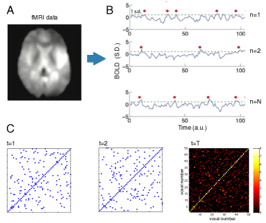
Figure 1 summarizes the basic process that has been used inT1 ; T2 ; T3 to define the point process in brain signals. The data consists in time series representing the activity of one of many thousands small brain regions, recorded from the brain using functional magnetic resonance imaging (fMRI). This imaging technique measures in each small region a “blood oxygenated level dependent” signal (i.e., “BOLD”), that is an estimation of the blood’ saturation of oxygen, which itself is proportional to the local neuronal activity. As shown in the figure, time points are selected at the upward threshold (here at unity) crossings of the signal (filled circles). The point process can be constructed also by selecting the local peaks of the BOLD time series. The temporal co-occurrence of the points defines the co-activation matrix (bottom graphs) which can be further averaged to estimate the correlation matrix of the system under study.

Figure 2: An example of the performance of the PP as a function of the number of points used. The “heat map” images represent the co-activation rates (in units of standard deviation, z-scores $Z$ ) of each voxel respect to the seed located at MNI coordinates x=4, y=-60, z=18. Different panels correspond to the results obtained using increasing number of points: 4, 7, 14 and 27, respectively. Note that a few points already suffice to identify well defined clusters that are 1-4 standard deviations away from chance co-activations. Red/ blue colors label positive/negative points co-activations, corresponding to positive/negative correlations.

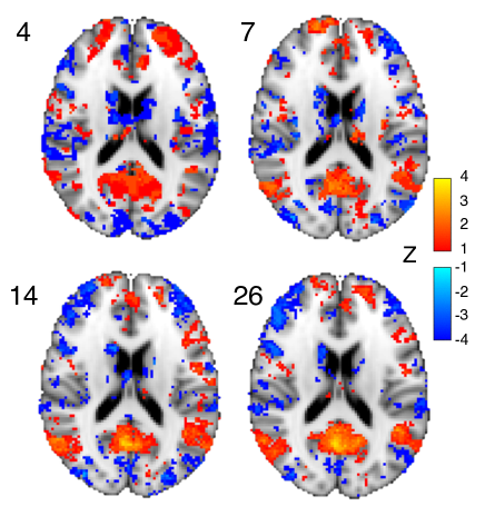
It has been established already, in different circumstancesT1 ; T2 ; T3 , that the co-activation matrix obtained with the PP methods is very similar to the correlation matrix computed from the full (i.e., continuous) BOLD signal. Since this implies a large compression, the question is why a few points are enough to compute results similar to those obtained with the full signal. Figure 2 shows an example constructed from BOLD time series from an experiment in which the subject is resting T3 . The results demonstrate that as few as 4 points are already sufficient to define clusters of co-activation, as demonstrated previously in T1 ; T2 ; T3 . In addition, the results here show how de-activations (i.e., blueish colors) are also evidenced by the PP approach.

A simple visual inspection of the BOLD traces reveals that the type of signals we are dealing with are temporally correlated. This is very well known, the neuronal activity is temporally and spatially correlated, and furthermore the activity is convoluted by the hemodynamic transfer function which in itself introduce additional temporal correlations. Therefore, for any time series with that properties, it seems natural to think that the most informative points are those in which its derivative changes sign. The rest of the points are redundant, since they can be predicted, up to a degree, by a linear estimator.

Figure 3: Why it works: The trace in Panel A is an example of a two minutes-long recording of a BOLD brain signal during rest. The point process is defined by the peaks and valleys, encompassed only by the six dots depicted in the bottom trace out of the 120 points of the time series. A piece-wise linear time series (dashed lines) is constructed by joining the peaks and valleys (two indicated by arrows) larger than a given threshold, here denoted by horizontal dotted lines. Panels D and E correspond to the computed similarity between the BOLD signals and the piece-wise linear signals (evaluated by the correlation $\langle r\rangle$ and error $rms_{e}$ values) for different autocorrelation $\gamma$ and threshold $\nu$ values. Panels B and C correspond to similar calculations for synthetic time series.

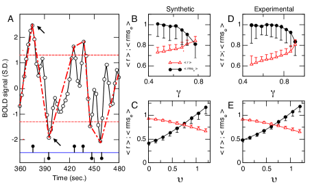
This is illustrated in Figure 3 using as an example two minutes of BOLD recording (normalized by its standard deviation (S.D)). After setting a threshold $\nu$ the inflection points larger than a given $\nu$ value are identified. These points constitutes the marked point process in question. Now we ask how much of the raw signal is left out if these points are used to extrapolate a piece-wise linear time series. To answer that we analyze BOLD time series from the brain of a subject during an experiment in which fMRI data is collected at restT2 . We proceed to compute the linear correlation between the two time series, the raw and the piece-wise linear one. In panels B and C are shown the results for different values of threshold $\nu$ (in units of S.D.) as well as for the correlation of the time series, estimated by the value of the first autocorrelation coefficient $\gamma$. Panel D shows that as the BOLD signal’ autocorrelation increases the similarity between the piece-wise linear and the raw signals increases, evaluated in two ways: by the $rms_{e}$ error and the linear correlation $\langle r\rangle$ between both time series. As expected, the raising of the threshold $\nu$ from zero (i.e, less information from the signal is considered) it is followed by a monotonic increase of the $rms_{e}$ and a decrease of the $\langle r\rangle$ values (see Panel E).

According with the present hypothesis, the functional dependences shown by the BOLD signals in Panel D and E shall be replicated by using synthetic signals with similar autocorrelation properties. For that we generate artificial time series with autocorrelation values identical to those of the BOLD signals using the routine _alpha_gaussian.m } rom MATLAB. Panels B and C show that the dependence with the threshold $\nu$ and $\gamma$ exhibit very similar behavior. The results show that the key lies in the correlation properties of the time series under consideration. In synthesis, it is found that signals with long range correlations are particularly suitable for this type of compression, where inflection points contains most of the information. The results shall apply as well to other signals from any origin as long as their autocorrelation features are similar.

In summary, the success and the merits of the PP approach to represent spatiotemporal dynamics are related to a very trivial fact: in the case of autocorrelated signals the only informative points are those with zero derivative (inflection points); remaining ones are more or less straight lines which can be in principle, and for certain applications, ignored. Applications of these ideas to a diversity of fields should be expected.

References

- (1) Tagliazucchi E, Balenzuela P, Fraiman D, Montoya P, Chialvo DR (2011). Spontaneous BOLD event triggered averages for estimating functional connectivity at resting state. Neurosci. Lett., 488(2), 158–163.
- (2) Tagliazucchi E, Balenzuela P, Fraiman D, Chialvo DR. (2012). Criticality in large-scale brain fMRI dynamics unveiled by a novel point process analysis. Front. Physiol., 3:15 https://doi.org/10.3389/fphys.2012.00015
- (3) Tagliazucchi E, Siniatchkin M, Helmut Laufs H, Chialvo DR.(2016). The voxel-wise functional connectome can be efficiently derived from co-activations in a sparse spatio-temporal point-process. Front. Neurosci. /doi.org/10.3389/fnins.2016.00381
- (4) Petridou N, Gaudes CC, Dryden IL, Francis ST, Gowland PA. (2013). Periods of rest in fMRI contain individual spontaneous events which are related to slowly fluctuating spontaneous activity. Hum. Brain. Mapp., 34(6), 1319–1329.
- (5) Allan TW, Francis ST, Caballero-Gaudes C, Morris PG, Liddle EB, Liddle PF, Brookes MJ, & Gowland PA (2015). Functional connectivity in MRI is driven by spontaneous BOLD events. PloS ONE, 10 (4).
- (6) Li W, Li Y, Hu C, Chen X, Dai H. (2014). Point process analysis in brain networks of patients with diabetes. Neurocomputing, 145, 182–189.
- (7) Liu X, Duyn JH. (2013). Time-varying functional network information extracted from brief instances of spontaneous brain activity. Proc. Natl. Acad. Sci. USA, 110(11), 4392–4397.
- (8) Liu X, Chang C, Duyn JH. (2013). Decomposition of spontaneous brain activity into distinct fMRI co-activation patterns. Front. Sys. Neurosci., 7:101
- (9) Chen JE, Chang C, Greicius MD, Glover GH. (2015). Introducing co-activation pattern metrics to quantify spontaneous brain network dynamics. NeuroImage doi:10.1016/j.neuroimage.2015.01.057.
- (10) Jiang X, Lv J, Zhu D, Zhang T, Hu X, Guo L, Liu T. (2014). Integrating group-wise functional brain activities via point processes. Biomedical Imaging (ISBI), 2014 IEEE 11th International Symposium on (pp. 669–672). IEEE.
- (11) Amico E., Gomez F., Di Perri C., Vanhaudenhuyse A., Lesenfants D., Boveroux P., et al. . (2014). Posterior cingulate cortex-related co-activation patterns: a resting state fMRI study in propofol-induced loss of consciousness. PLoS ONE 9:e100012. 10.1371/journal.pone.0100012
- (12) Wu G. R., Liao W., Stramaglia S., Ding J. R., Chen H., Marinazzo D. (2013). A blind deconvolution approach to recover effective connectivity brain networks from resting state fMRI data. Med. Image Anal. 17, 365–374. 10.1016/j.media.2013.01.003
- (13) Cordes D, Haughton V, Carew J. D., Arfanakis K., Maravilla K. (2002). Hierarchical clustering to measure connectivity in fMRI resting-state data. Magn. Reson. Imaging 20, 305-317. 10.1016/S0730-725X(02)00503-9