Noisy Networks for Exploration
Abstract
We introduce NoisyNet, a deep reinforcement learning agent with parametric noise added to its weights, and show that the induced stochasticity of the agent’s policy can be used to aid efficient exploration. The parameters of the noise are learned with gradient descent along with the remaining network weights. NoisyNet is straightforward to implement and adds little computational overhead. We find that replacing the conventional exploration heuristics for A3C, DQN and Dueling agents (entropy reward and -greedy respectively) with NoisyNet yields substantially higher scores for a wide range of Atari games, in some cases advancing the agent from sub to super-human performance.
1 Introduction
Despite the wealth of research into efficient methods for exploration in Reinforcement Learning (RL) (Kearns & Singh, 2002; Jaksch et al., 2010), most exploration heuristics rely on random perturbations of the agent’s policy, such as -greedy (Sutton & Barto, 1998) or entropy regularisation (Williams, 1992), to induce novel behaviours. However such local ‘dithering’ perturbations are unlikely to lead to the large-scale behavioural patterns needed for efficient exploration in many environments (Osband et al., 2017).
Optimism in the face of uncertainty is a common exploration heuristic in reinforcement learning. Various forms of this heuristic often come with theoretical guarantees on agent performance (Azar et al., 2017; Lattimore et al., 2013; Jaksch et al., 2010; Auer & Ortner, 2007; Kearns & Singh, 2002). However, these methods are often limited to small state-action spaces or to linear function approximations and are not easily applied with more complicated function approximators such as neural networks (except from work by (Geist & Pietquin, 2010a; b) but it doesn’t come with convergence guarantees). A more structured approach to exploration is to augment the environment’s reward signal with an additional intrinsic motivation term (Singh et al., 2004) that explicitly rewards novel discoveries. Many such terms have been proposed, including learning progress (Oudeyer & Kaplan, 2007), compression progress (Schmidhuber, 2010), variational information maximisation (Houthooft et al., 2016) and prediction gain (Bellemare et al., 2016). One problem is that these methods separate the mechanism of generalisation from that of exploration; the metric for intrinsic reward, and–importantly–its weighting relative to the environment reward, must be chosen by the experimenter, rather than learned from interaction with the environment. Without due care, the optimal policy can be altered or even completely obscured by the intrinsic rewards; furthermore, dithering perturbations are usually needed as well as intrinsic reward to ensure robust exploration (Ostrovski et al., 2017). Exploration in the policy space itself, for example, with evolutionary or black box algorithms (Moriarty et al., 1999; Fix & Geist, 2012; Salimans et al., 2017), usually requires many prolonged interactions with the environment. Although these algorithms are quite generic and can apply to any type of parametric policies (including neural networks), they are usually not data efficient and require a simulator to allow many policy evaluations.
We propose a simple alternative approach, called NoisyNet, where learned perturbations of the network weights are used to drive exploration. The key insight is that a single change to the weight vector can induce a consistent, and potentially very complex, state-dependent change in policy over multiple time steps – unlike dithering approaches where decorrelated (and, in the case of -greedy, state-independent) noise is added to the policy at every step. The perturbations are sampled from a noise distribution. The variance of the perturbation is a parameter that can be considered as the energy of the injected noise. These variance parameters are learned using gradients from the reinforcement learning loss function, along side the other parameters of the agent. The approach differs from parameter compression schemes such as variational inference (Hinton & Van Camp, 1993; Bishop, 1995; Graves, 2011; Blundell et al., 2015; Gal & Ghahramani, 2016) and flat minima search (Hochreiter & Schmidhuber, 1997) since we do not maintain an explicit distribution over weights during training but simply inject noise in the parameters and tune its intensity automatically. Consequently, it also differs from Thompson sampling (Thompson, 1933; Lipton et al., 2016) as the distribution on the parameters of our agents does not necessarily converge to an approximation of a posterior distribution.
At a high level our algorithm is a randomised value function, where the functional form is a neural network. Randomised value functions provide a provably efficient means of exploration (Osband et al., 2014). Previous attempts to extend this approach to deep neural networks required many duplicates of sections of the network (Osband et al., 2016). By contrast in our NoisyNet approach while the number of parameters in the linear layers of the network is doubled, as the weights are a simple affine transform of the noise, the computational complexity is typically still dominated by the weight by activation multiplications, rather than the cost of generating the weights. Additionally, it also applies to policy gradient methods such as A3C out of the box (Mnih et al., 2016). Most recently (and independently of our work) Plappert et al. (2017) presented a similar technique where constant Gaussian noise is added to the parameters of the network. Our method thus differs by the ability of the network to adapt the noise injection with time and it is not restricted to Gaussian noise distributions. We need to emphasise that the idea of injecting noise to improve the optimisation process has been thoroughly studied in the literature of supervised learning and optimisation under different names (e.g., Neural diffusion process (Mobahi, 2016) and graduated optimisation (Hazan et al., 2016)). These methods often rely on a noise of vanishing size that is non-trainable, as opposed to NoisyNet which tunes the amount of noise by gradient descent.
NoisyNet can also be adapted to any deep RL algorithm and we demonstrate this versatility by providing NoisyNet versions of DQN (Mnih et al., 2015), Dueling (Wang et al., 2016) and A3C (Mnih et al., 2016) algorithms. Experiments on 57 Atari games show that NoisyNet-DQN and NoisyNetDueling achieve striking gains when compared to the baseline algorithms without significant extra computational cost, and with less hyper parameters to tune. Also the noisy version of A3C provides some improvement over the baseline.
2 Background
This section provides mathematical background for Markov Decision Processes (MDPs) and deep RL with Q-learning, dueling and actor-critic methods.
2.1 Markov Decision Processes and Reinforcement Learning
MDPs model stochastic, discrete-time and finite action space control problems (Bellman & Kalaba, 1965; Bertsekas, 1995; Puterman, 1994). An MDP is a tuple where is the state space, the action space, the reward function, the discount factor and a stochastic kernel modelling the one-step Markovian dynamics ( is the probability of transitioning to state by choosing action in state ). A stochastic policy maps each state to a distribution over actions and gives the probability of choosing action in state . The quality of a policy is assessed by the action-value function defined as:
| (1) |
where is the expectation over the distribution of the admissible trajectories obtained by executing the policy starting from and . Therefore, the quantity represents the expected -discounted cumulative reward collected by executing the policy starting from and . A policy is optimal if no other policy yields a higher return. The action-value function of the optimal policy is .
The value function for a policy is defined as , and represents the expected -discounted return collected by executing the policy starting from state .
2.2 Deep Reinforcement Learning
Deep Reinforcement Learning uses deep neural networks as function approximators for RL methods. Deep Q-Networks (DQN) (Mnih et al., 2015), Dueling architecture (Wang et al., 2016), Asynchronous Advantage Actor-Critic (A3C) (Mnih et al., 2016), Trust Region Policy Optimisation (Schulman et al., 2015), Deep Deterministic Policy Gradient (Lillicrap et al., 2015) and distributional RL (C51) (Bellemare et al., 2017) are examples of such algorithms. They frame the RL problem as the minimisation of a loss function , where represents the parameters of the network. In our experiments we shall consider the DQN, Dueling and A3C algorithms.
DQN (Mnih et al., 2015) uses a neural network as an approximator for the action-value function of the optimal policy . DQN’s estimate of the optimal action-value function, , is found by minimising the following loss with respect to the neural network parameters :
| (2) |
where is a distribution over transitions drawn from a replay buffer of previously observed transitions. Here represents the parameters of a fixed and separate target network which is updated () regularly to stabilise the learning. An -greedy policy is used to pick actions greedily according to the action-value function or, with probability , a random action is taken.
The Dueling DQN (Wang et al., 2016) is an extension of the DQN architecture. The main difference is in using Dueling network architecture as opposed to the Q network in DQN. Dueling network estimates the action-value function using two parallel sub-networks, the value and advantage sub-network, sharing a convolutional layer. Let , , and be, respectively, the parameters of the convolutional encoder , of the value network , and of the advantage network ; and is their concatenation. The output of these two networks are combined as follows for every :
| (3) |
The Dueling algorithm then makes use of the double-DQN update rule (van Hasselt et al., 2016) to optimise :
| (4) | ||||
| (5) |
where the definition distribution and the target network parameter set is identical to DQN.
In contrast to DQN and Dueling, A3C (Mnih et al., 2016) is a policy gradient algorithm. A3C’s network directly learns a policy and a value function of its policy. The gradient of the loss on the A3C policy at step for the roll-out is:
| (6) |
denotes the entropy of the policy and is a hyper parameter that trades off between optimising the advantage function and the entropy of the policy. The advantage function is the difference between observed returns and estimates of the return produced by A3C’s value network: , being the reward at step and being the agent’s estimate of value function of state .
The parameters of the value function are found to match on-policy returns; namely we have
| (7) |
where is the return obtained by executing policy starting in state . In practice, and as in Mnih et al. (2016), we estimate as where are rewards observed by the agent, and is the th state observed when starting from observed state . The overall A3C loss is then where balances optimising the policy loss relative to the baseline value function loss.
3 NoisyNets for Reinforcement Learning
NoisyNets are neural networks whose weights and biases are perturbed by a parametric function of the noise. These parameters are adapted with gradient descent. More precisely, let be a neural network parameterised by the vector of noisy parameters which takes the input and outputs . We represent the noisy parameters as , where is a set of vectors of learnable parameters, is a vector of zero-mean noise with fixed statistics and represents element-wise multiplication. The usual loss of the neural network is wrapped by expectation over the noise : . Optimisation now occurs with respect to the set of parameters .
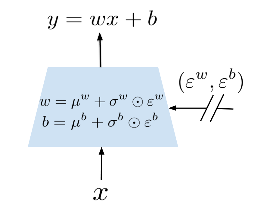
Consider a linear layer of a neural network with inputs and outputs, represented by
| (8) |
where is the layer input, the weight matrix, and the bias. The corresponding noisy linear layer is defined as:
| (9) |
where and replace and in Eq. (8), respectively. The parameters , , and are learnable whereas and are noise random variables (the specific choices of this distribution are described below). We provide a graphical representation of a noisy linear layer in Fig. 4 (see Appendix B).
We now turn to explicit instances of the noise distributions for linear layers in a noisy network. We explore two options: Independent Gaussian noise, which uses an independent Gaussian noise entry per weight and Factorised Gaussian noise, which uses an independent noise per each output and another independent noise per each input. The main reason to use factorised Gaussian noise is to reduce the compute time of random number generation in our algorithms. This computational overhead is especially prohibitive in the case of single-thread agents such as DQN and Duelling. For this reason we use factorised noise for DQN and Duelling and independent noise for the distributed A3C, for which the compute time is not a major concern.
-
(a)
Independent Gaussian noise: the noise applied to each weight and bias is independent, where each entry (respectively each entry ) of the random matrix (respectively of the random vector ) is drawn from a unit Gaussian distribution. This means that for each noisy linear layer, there are noise variables (for inputs to the layer and outputs).
-
(b)
Factorised Gaussian noise: by factorising , we can use unit Gaussian variables for noise of the inputs and and unit Gaussian variables for noise of the outputs (thus unit Gaussian variables in total). Each and can then be written as:
(10) (11) where is a real-valued function. In our experiments we used . Note that for the bias Eq. (11) we could have set , but we decided to keep the same output noise for weights and biases.
Since the loss of a noisy network, , is an expectation over the noise, the gradients are straightforward to obtain:
| (12) |
We use a Monte Carlo approximation to the above gradients, taking a single sample at each step of optimisation:
| (13) |
3.1 Deep Reinforcement Learning with NoisyNets
We now turn to our application of noisy networks to exploration in deep reinforcement learning. Noise drives exploration in many methods for reinforcement learning, providing a source of stochasticity external to the agent and the RL task at hand. Either the scale of this noise is manually tuned across a wide range of tasks (as is the practice in general purpose agents such as DQN or A3C) or it can be manually scaled per task. Here we propose automatically tuning the level of noise added to an agent for exploration, using the noisy networks training to drive down (or up) the level of noise injected into the parameters of a neural network, as needed.
A noisy network agent samples a new set of parameters after every step of optimisation. Between optimisation steps, the agent acts according to a fixed set of parameters (weights and biases). This ensures that the agent always acts according to parameters that are drawn from the current noise distribution.
Deep Q-Networks (DQN) and Dueling.
We apply the following modifications to both DQN and Dueling: first, -greedy is no longer used, but instead the policy greedily optimises the (randomised) action-value function. Secondly, the fully connected layers of the value network are parameterised as a noisy network, where the parameters are drawn from the noisy network parameter distribution after every replay step. We used factorised Gaussian noise as explained in (b) from Sec. 3. For replay, the current noisy network parameter sample is held fixed across the batch. Since DQN and Dueling take one step of optimisation for every action step, the noisy network parameters are re-sampled before every action. We call the new adaptations of DQN and Dueling, NoisyNet-DQN and NoisyNet-Dueling, respectively.
We now provide the details of the loss function that our variant of DQN is minimising. When replacing the linear layers by noisy layers in the network (respectively in the target network), the parameterised action-value function (respectively ) can be seen as a random variable and the DQN loss becomes the NoisyNet-DQN loss:
| (14) |
where the outer expectation is with respect to distribution of the noise variables for the noisy value function and the noise variable for the noisy target value function . Computing an unbiased estimate of the loss is straightforward as we only need to compute, for each transition in the replay buffer, one instance of the target network and one instance of the online network. We generate these independent noises to avoid bias due to the correlation between the noise in the target network and the online network. Concerning the action choice, we generate another independent sample for the online network and we act greedily with respect to the corresponding output action-value function.
Similarly the loss function for NoisyNet-Dueling is defined as:
| (15) | ||||
| (16) |
Both algorithms are provided in Appendix C.1.
Asynchronous Advantage Actor Critic (A3C).
A3C is modified in a similar fashion to DQN: firstly, the entropy bonus of the policy loss is removed. Secondly, the fully connected layers of the policy network are parameterised as a noisy network. We used independent Gaussian noise as explained in (a) from Sec. 3. In A3C, there is no explicit exploratory action selection scheme (such as -greedy); and the chosen action is always drawn from the current policy. For this reason, an entropy bonus of the policy loss is often added to discourage updates leading to deterministic policies. However, when adding noisy weights to the network, sampling these parameters corresponds to choosing a different current policy which naturally favours exploration. As a consequence of direct exploration in the policy space, the artificial entropy loss on the policy can thus be omitted. New parameters of the policy network are sampled after each step of optimisation, and since A3C uses step returns, optimisation occurs every steps. We call this modification of A3C, NoisyNet-A3C.
Indeed, when replacing the linear layers by noisy linear layers (the parameters of the noisy network are now noted ), we obtain the following estimation of the return via a roll-out of size :
| (17) |
As A3C is an on-policy algorithm the gradients are unbiased when noise of the network is consistent for the whole roll-out. Consistency among action value functions is ensured by letting letting the noise be the same throughout each rollout, i.e., . Additional details are provided in the Appendix A and the algorithm is given in Appendix C.2.
3.2 Initialisation of Noisy Networks
In the case of an unfactorised noisy networks, the parameters and are initialised as follows. Each element is sampled from independent uniform distributions , where is the number of inputs to the corresponding linear layer, and each element is simply set to for all parameters. This particular initialisation was chosen because similar values worked well for the supervised learning tasks described in Fortunato et al. (2017), where the initialisation of the variances of the posteriors and the variances of the prior are related. We have not tuned for this parameter, but we believe different values on the same scale should provide similar results.
For factorised noisy networks, each element was initialised by a sample from an independent uniform distributions and each element was initialised to a constant . The hyperparameter is set to .
4 Results


We evaluated the performance of noisy network agents on 57 Atari games (Bellemare et al., 2015) and compared to baselines that, without noisy networks, rely upon the original exploration methods (-greedy and entropy bonus).
4.1 Training details and performance
We used the random start no-ops scheme for training and evaluation as described the original DQN paper (Mnih et al., 2015). The mode of evaluation is identical to those of Mnih et al. (2016) where randomised restarts of the games are used for evaluation after training has happened. The raw average scores of the agents are evaluated during training, every 1M frames in the environment, by suspending learning and evaluating the latest agent for 500K frames. Episodes are truncated at 108K frames (or 30 minutes of simulated play) (van Hasselt et al., 2016).
We consider three baseline agents: DQN (Mnih et al., 2015), duel clip variant of Dueling algorithm (Wang et al., 2016) and A3C (Mnih et al., 2016). The DQN and A3C agents were training for 200M and 320M frames, respectively. In each case, we used the neural network architecture from the corresponding original papers for both the baseline and NoisyNet variant. For the NoisyNet variants we used the same hyper parameters as in the respective original paper for the baseline.
We compared absolute performance of agents using the human normalised score:
| (18) |
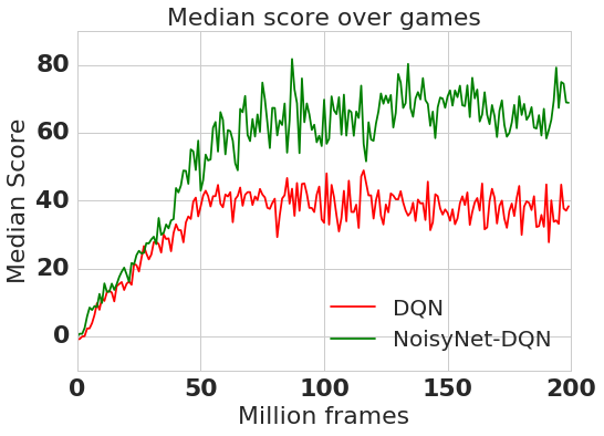
where human and random scores are the same as those in Wang et al. (2016). Note that the human normalised score is zero for a random agent and for human level performance. Per-game maximum scores are computed by taking the maximum raw scores of the agent and then averaging over three seeds. However, for computing the human normalised scores in Figure 2, the raw scores are evaluated every 1M frames and averaged over three seeds. The overall agent performance is measured by both mean and median of the human normalised score across all 57 Atari games.
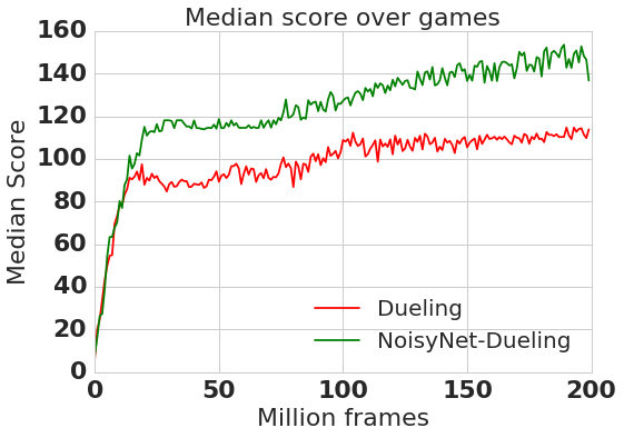
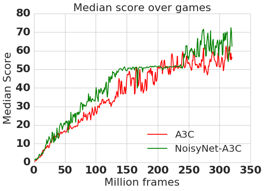
The aggregated results across all 57 Atari games are reported in Table 1, while the individual scores for each game are in Table 3 from the Appendix E. The median human normalised score is improved in all agents by using NoisyNet, adding at least (in the case of A3C) and at most (in the case of DQN) percentage points to the median human normalised score. The mean human normalised score is also significantly improved for all agents. Interestingly the Dueling case, which relies on multiple modifications of DQN, demonstrates that NoisyNet is orthogonal to several other improvements made to DQN.
| Baseline | NoisyNet | Improvement | |||
|---|---|---|---|---|---|
| Mean | Median | Mean | Median | (On median) | |
| DQN | 319 | 83 | 379 | 123 | 48% |
| Dueling | 524 | 132 | 633 | 172 | 30% |
| A3C | 293 | 80 | 347 | 94 | 18% |
We also compared relative performance of NoisyNet agents to the respective baseline agent without noisy networks:
| (19) |
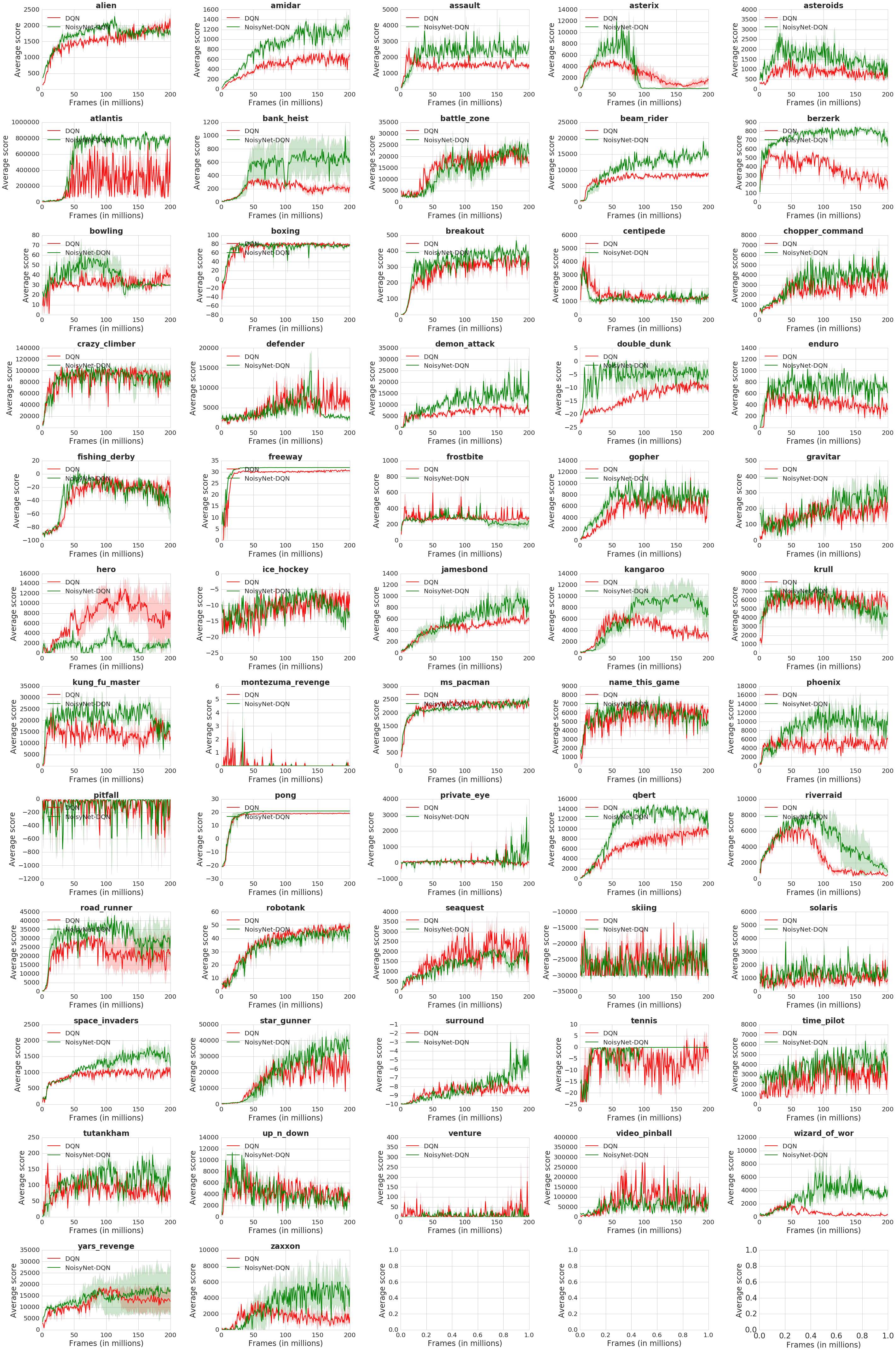
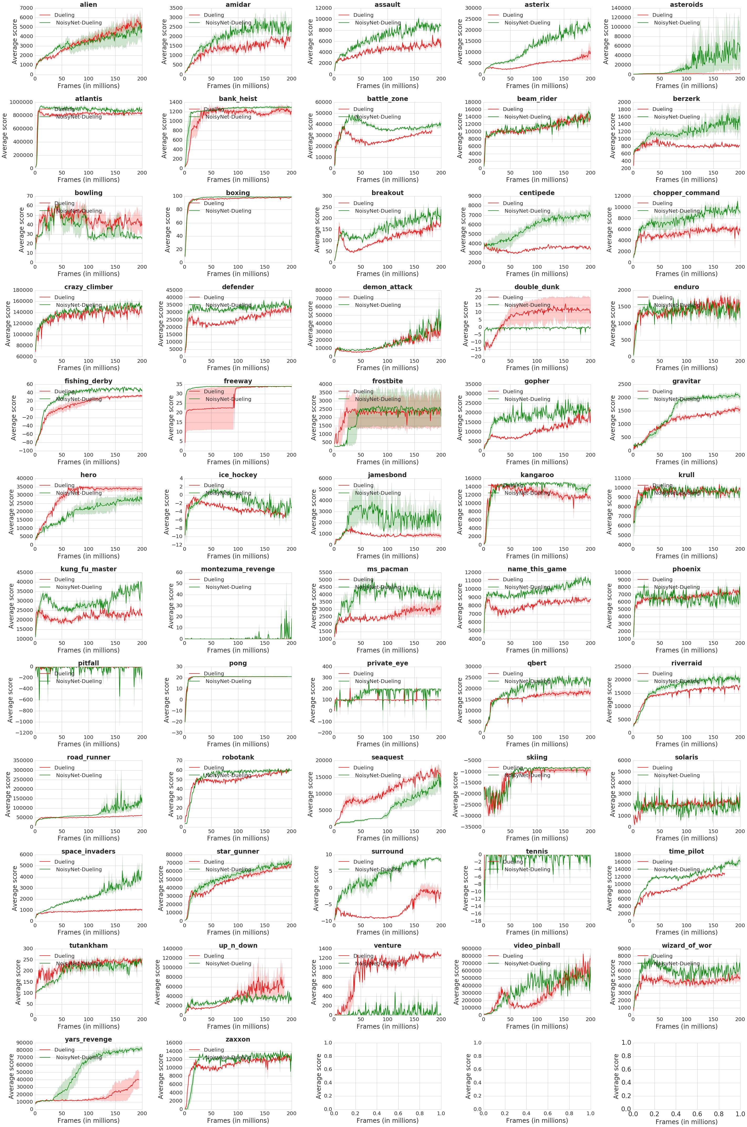
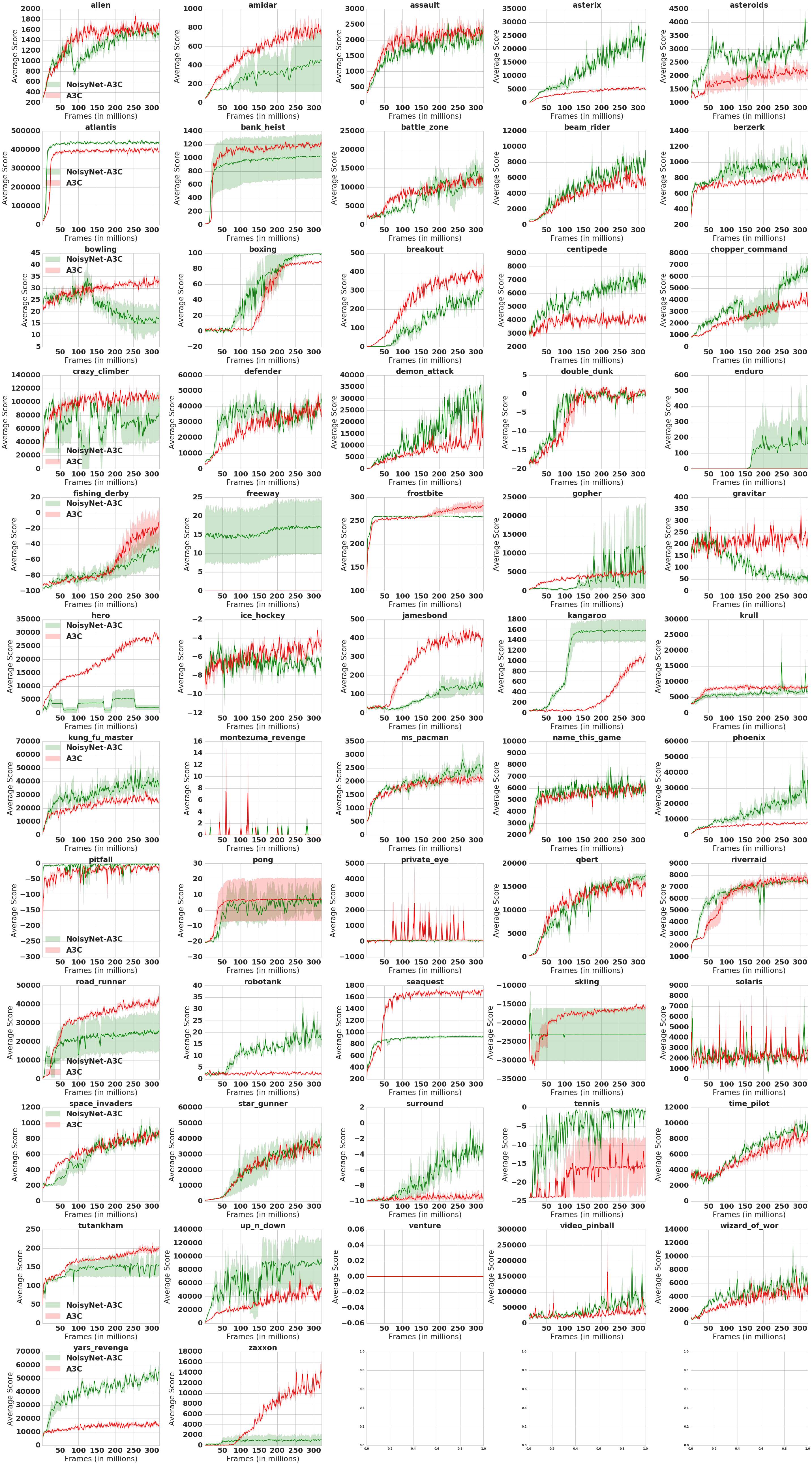
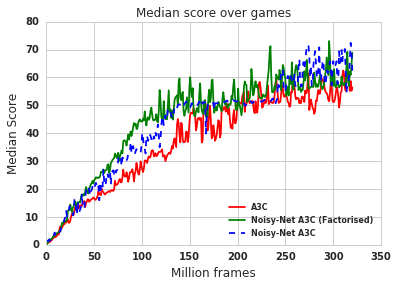
As before, the per-game score is computed by taking the maximum performance for each game and then averaging over three seeds. The relative human normalised scores are shown in Figure 1. As can be seen, the performance of NoisyNet agents (DQN, Dueling and A3C) is better for the majority of games relative to the corresponding baseline, and in some cases by a considerable margin. Also as it is evident from the learning curves of Fig. 2 NoisyNet agents produce superior performance compared to their corresponding baselines throughout the learning process. This improvement is especially significant in the case of NoisyNet-DQN and NoisyNet-Dueling. Also in some games, NoisyNet agents provide an order of magnitude improvement on the performance of the vanilla agent; as can be seen in Table 3 in the Appendix E with detailed breakdown of individual game scores and the learning curves plots from Figs 6, 7 and 8, for DQN, Dueling and A3C, respectively. We also ran some experiments evaluating the performance of NoisyNet-A3C with factorised noise. We report the corresponding learning curves and the scores in Fig. LABEL:fig:learning_curves_median_factorised and Table 2, respectively (see Appendix D). This result shows that using factorised noise does not lead to any significant decrease in the performance of A3C. On the contrary it seems that it has positive effects in terms of improving the median score as well as speeding up the learning process.
4.2 Analysis of Learning in Noisy Layers
In this subsection, we try to provide some insight on how noisy networks affect the learning process and the exploratory behaviour of the agent. In particular, we focus on analysing the evolution of the noise weights and throughout the learning process. We first note that, as is a positive and continuous function of , there always exists a deterministic optimiser for the loss (defined in Eq. (14)). Therefore, one may expect that, to obtain the deterministic optimal solution, the neural network may learn to discard the noise entries by eventually pushing s and towards .
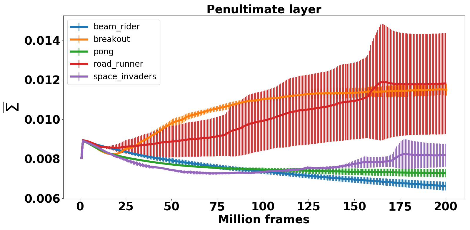
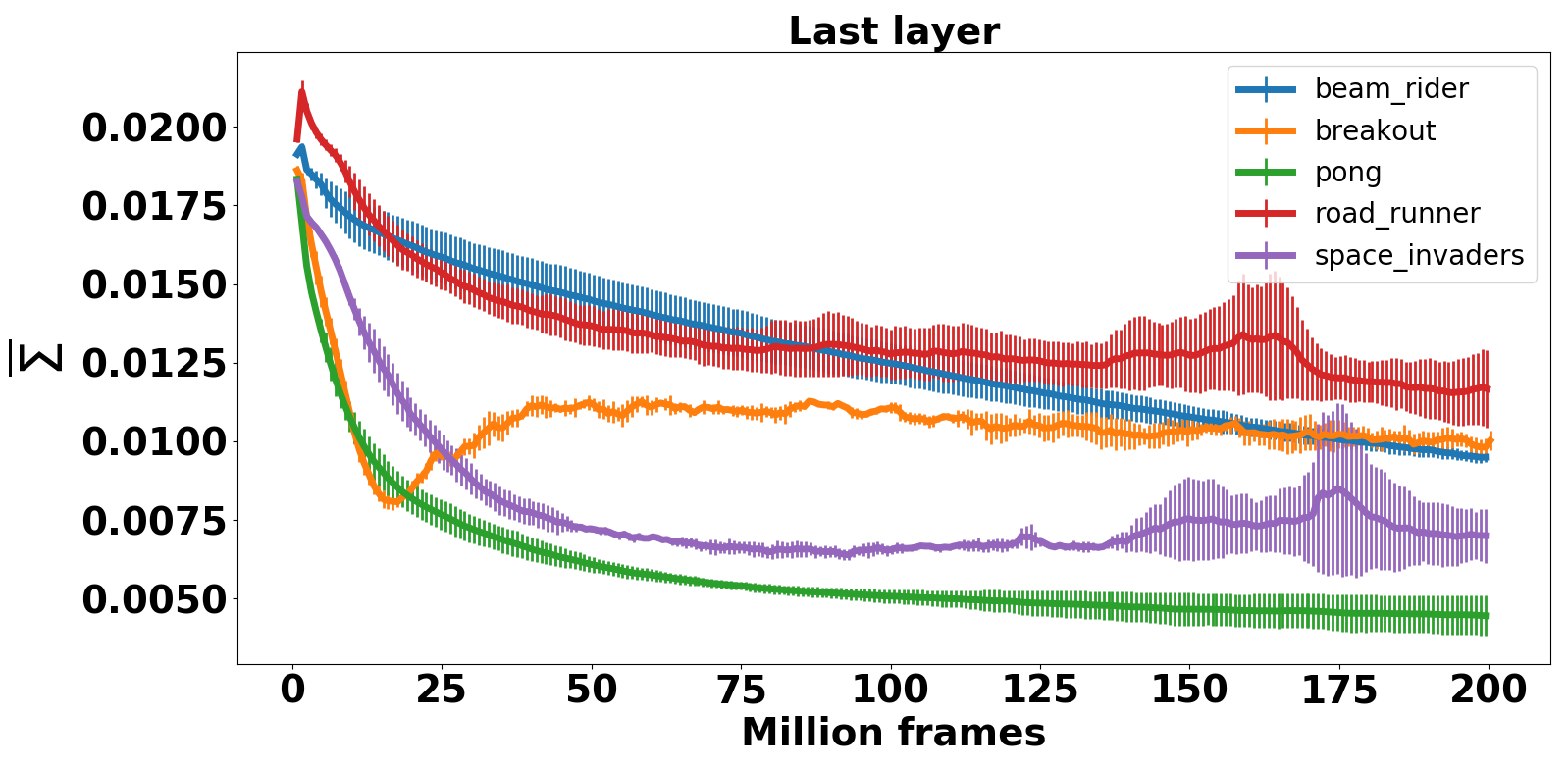
To test this hypothesis we track the changes in s throughout the learning process. Let denote the weight of a noisy layer. We then define , the mean-absolute of the s of a noisy layer, as
| (20) |
Intuitively speaking provides some measure of the stochasticity of the Noisy layers. We report the learning curves of the average of across seeds in Fig. 3 for a selection of Atari games in NoisyNet-DQN agent. We observe that of the last layer of the network decreases as the learning proceeds in all cases, whereas in the case of the penultimate layer this only happens for 2 games out of 5 (Pong and Beam rider) and in the remaining 3 games in fact increases. This shows that in the case of NoisyNet-DQN the agent does not necessarily evolve towards a deterministic solution as one might have expected. Another interesting observation is that the way evolves significantly differs from one game to another and in some cases from one seed to another seed, as it is evident from the error bars. This suggests that NoisyNet produces a problem-specific exploration strategy as opposed to fixed exploration strategy used in standard DQN.
5 Conclusion
We have presented a general method for exploration in deep reinforcement learning that shows significant performance improvements across many Atari games in three different agent architectures. In particular, we observe that in games such as Beam rider, Asteroids and Freeway that the standard DQN, Dueling and A3C perform poorly compared with the human player, NoisyNet-DQN, NoisyNet-Dueling and NoisyNet-A3C achieve super human performance, respectively. Although the improvements in performance might also come from the optimisation aspect since the cost functions are modified, the uncertainty in the parameters of the networks introduced by NoisyNet is the only exploration mechanism of the method. Having weights with greater uncertainty introduces more variability into the decisions made by the policy, which has potential for exploratory actions, but further analysis needs to be done in order to disentangle the exploration and optimisation effects.
Another advantage of NoisyNet is that the amount of noise injected in the network is tuned automatically by the RL algorithm. This alleviates the need for any hyper parameter tuning (required with standard entropy bonus and -greedy types of exploration). This is also in contrast to many other methods that add intrinsic motivation signals that may destabilise learning or change the optimal policy. Another interesting feature of the NoisyNet approach is that the degree of exploration is contextual and varies from state to state based upon per-weight variances. While more gradients are needed, the gradients on the mean and variance parameters are related to one another by a computationally efficient affine function, thus the computational overhead is marginal. Automatic differentiation makes implementation of our method a straightforward adaptation of many existing methods. A similar randomisation technique can also be applied to LSTM units (Fortunato et al., 2017) and is easily extended to reinforcement learning, we leave this as future work.
Note NoisyNet exploration strategy is not restricted to the baselines considered in this paper. In fact, this idea can be applied to any deep RL algorithms that can be trained with gradient descent, including DDPG (Lillicrap et al., 2015), TRPO (Schulman et al., 2015) or distributional RL (C51) (Bellemare et al., 2017). As such we believe this work is a step towards the goal of developing a universal exploration strategy.
Acknowledgements
We would like to thank Koray Kavukcuoglu, Oriol Vinyals, Daan Wierstra, Georg Ostrovski, Joseph Modayil, Simon Osindero, Chris Apps, Stephen Gaffney and many others at DeepMind for insightful discussions, comments and feedback on this work.
References
- Auer & Ortner (2007) Peter Auer and Ronald Ortner. Logarithmic online regret bounds for undiscounted reinforcement learning. Advances in Neural Information Processing Systems, 19:49, 2007.
- Azar et al. (2017) Mohammad Gheshlaghi Azar, Ian Osband, and Rémi Munos. Minimax regret bounds for reinforcement learning. arXiv preprint arXiv:1703.05449, 2017.
- Bellemare et al. (2015) Marc Bellemare, Yavar Naddaf, Joel Veness, and Michael Bowling. The arcade learning environment: An evaluation platform for general agents. In Twenty-Fourth International Joint Conference on Artificial Intelligence, 2015.
- Bellemare et al. (2016) Marc Bellemare, Sriram Srinivasan, Georg Ostrovski, Tom Schaul, David Saxton, and Remi Munos. Unifying count-based exploration and intrinsic motivation. In Advances in Neural Information Processing Systems, pp. 1471–1479, 2016.
- Bellemare et al. (2017) Marc G Bellemare, Will Dabney, and Rémi Munos. A distributional perspective on reinforcement learning. In International Conference on Machine Learning, pp. 449–458, 2017.
- Bellman & Kalaba (1965) Richard Bellman and Robert Kalaba. Dynamic programming and modern control theory. Academic Press New York, 1965.
- Bertsekas (1995) Dimitri Bertsekas. Dynamic programming and optimal control, volume 1. Athena Scientific, Belmont, MA, 1995.
- Bishop (1995) Chris M Bishop. Training with noise is equivalent to Tikhonov regularization. Neural computation, 7(1):108–116, 1995.
- Blundell et al. (2015) Charles Blundell, Julien Cornebise, Koray Kavukcuoglu, and Daan Wierstra. Weight uncertainty in neural networks. In Proceedings of The 32nd International Conference on Machine Learning, pp. 1613–1622, 2015.
- Fix & Geist (2012) Jeremy Fix and Matthieu Geist. Monte-Carlo swarm policy search. In Swarm and Evolutionary Computation, pp. 75–83. Springer, 2012.
- Fortunato et al. (2017) Meire Fortunato, Charles Blundell, and Oriol Vinyals. Bayesian recurrent neural networks. arXiv preprint arXiv:1704.02798, 2017.
- Gal & Ghahramani (2016) Yarin Gal and Zoubin Ghahramani. Dropout as a bayesian approximation: Representing model uncertainty in deep learning. In Maria Florina Balcan and Kilian Q. Weinberger (eds.), Proceedings of The 33rd International Conference on Machine Learning, volume 48 of Proceedings of Machine Learning Research, pp. 1050–1059, New York, New York, USA, 20–22 Jun 2016. PMLR. URL http://proceedings.mlr.press/v48/gal16.html.
- Geist & Pietquin (2010a) Matthieu Geist and Olivier Pietquin. Kalman temporal differences. Journal of artificial intelligence research, 39:483–532, 2010a.
- Geist & Pietquin (2010b) Matthieu Geist and Olivier Pietquin. Managing uncertainty within value function approximation in reinforcement learning. In Active Learning and Experimental Design workshop (collocated with AISTATS 2010), Sardinia, Italy, volume 92, 2010b.
- Graves (2011) Alex Graves. Practical variational inference for neural networks. In Advances in Neural Information Processing Systems, pp. 2348–2356, 2011.
- Hazan et al. (2016) Elad Hazan, Kfir Yehuda Levy, and Shai Shalev-Shwartz. On graduated optimization for stochastic non-convex problems. In International Conference on Machine Learning, pp. 1833–1841, 2016.
- Hinton & Van Camp (1993) Geoffrey E Hinton and Drew Van Camp. Keeping the neural networks simple by minimizing the description length of the weights. In Proceedings of the sixth annual conference on Computational learning theory, pp. 5–13. ACM, 1993.
- Hochreiter & Schmidhuber (1997) Sepp Hochreiter and Jürgen Schmidhuber. Flat minima. Neural Computation, 9(1):1–42, 1997.
- Houthooft et al. (2016) Rein Houthooft, Xi Chen, Yan Duan, John Schulman, Filip De Turck, and Pieter Abbeel. VIME: Variational information maximizing exploration. In Advances in Neural Information Processing Systems, pp. 1109–1117, 2016.
- Jaksch et al. (2010) Thomas Jaksch, Ronald Ortner, and Peter Auer. Near-optimal regret bounds for reinforcement learning. Journal of Machine Learning Research, 11(Apr):1563–1600, 2010.
- Kearns & Singh (2002) Michael Kearns and Satinder Singh. Near-optimal reinforcement learning in polynomial time. Machine Learning, 49(2-3):209–232, 2002.
- Lattimore et al. (2013) Tor Lattimore, Marcus Hutter, and Peter Sunehag. The sample-complexity of general reinforcement learning. In Proceedings of The 30th International Conference on Machine Learning, pp. 28–36, 2013.
- Lillicrap et al. (2015) Timothy P Lillicrap, Jonathan J Hunt, Alexander Pritzel, Nicolas Heess, Tom Erez, Yuval Tassa, David Silver, and Daan Wierstra. Continuous control with deep reinforcement learning. arXiv preprint arXiv:1509.02971, 2015.
- Lipton et al. (2016) Zachary C Lipton, Jianfeng Gao, Lihong Li, Xiujun Li, Faisal Ahmed, and Li Deng. Efficient exploration for dialogue policy learning with BBQ networks & replay buffer spiking. arXiv preprint arXiv:1608.05081, 2016.
- Mnih et al. (2015) Volodymyr Mnih, Koray Kavukcuoglu, David Silver, Andrei A Rusu, Joel Veness, Marc G Bellemare, Alex Graves, Martin Riedmiller, Andreas K Fidjeland, Georg Ostrovski, et al. Human-level control through deep reinforcement learning. Nature, 518(7540):529–533, 2015.
- Mnih et al. (2016) Volodymyr Mnih, Adria Puigdomenech Badia, Mehdi Mirza, Alex Graves, Timothy Lillicrap, Tim Harley, David Silver, and Koray Kavukcuoglu. Asynchronous methods for deep reinforcement learning. In International Conference on Machine Learning, pp. 1928–1937, 2016.
- Mobahi (2016) Hossein Mobahi. Training recurrent neural networks by diffusion. arXiv preprint arXiv:1601.04114, 2016.
- Moriarty et al. (1999) David E Moriarty, Alan C Schultz, and John J Grefenstette. Evolutionary algorithms for reinforcement learning. Journal of Artificial Intelligence Research, 11:241–276, 1999.
- Osband et al. (2014) Ian Osband, Benjamin Van Roy, and Zheng Wen. Generalization and exploration via randomized value functions. arXiv preprint arXiv:1402.0635, 2014.
- Osband et al. (2016) Ian Osband, Charles Blundell, Alexander Pritzel, and Benjamin Van Roy. Deep exploration via bootstrapped DQN. In Advances In Neural Information Processing Systems, pp. 4026–4034, 2016.
- Osband et al. (2017) Ian Osband, Daniel Russo, Zheng Wen, and Benjamin Van Roy. Deep exploration via randomized value functions. arXiv preprint arXiv:1703.07608, 2017.
- Ostrovski et al. (2017) Georg Ostrovski, Marc G Bellemare, Aaron van den Oord, and Remi Munos. Count-based exploration with neural density models. arXiv preprint arXiv:1703.01310, 2017.
- Oudeyer & Kaplan (2007) Pierre-Yves Oudeyer and Frederic Kaplan. What is intrinsic motivation? A typology of computational approaches. Frontiers in neurorobotics, 1, 2007.
- Plappert et al. (2017) Matthias Plappert, Rein Houthooft, Prafulla Dhariwal, Szymon Sidor, Richard Y Chen, Xi Chen, Tamim Asfour, Pieter Abbeel, and Marcin Andrychowicz. Parameter space noise for exploration. arXiv preprint arXiv:1706.01905, 2017.
- Puterman (1994) Martin Puterman. Markov decision processes: discrete stochastic dynamic programming. John Wiley & Sons, 1994.
- Salimans et al. (2017) Tim Salimans, J. Ho, X. Chen, and I. Sutskever. Evolution Strategies as a Scalable Alternative to Reinforcement Learning. ArXiv e-prints, 2017.
- Schmidhuber (2010) Jürgen Schmidhuber. Formal theory of creativity, fun, and intrinsic motivation (1990–2010). IEEE Transactions on Autonomous Mental Development, 2(3):230–247, 2010.
- Schulman et al. (2015) J. Schulman, S. Levine, P. Abbeel, M. Jordan, and P. Moritz. Trust region policy optimization. In Proc. of ICML, pp. 1889–1897, 2015.
- Singh et al. (2004) Satinder P Singh, Andrew G Barto, and Nuttapong Chentanez. Intrinsically motivated reinforcement learning. In NIPS, volume 17, pp. 1281–1288, 2004.
- Sutton & Barto (1998) Richard S Sutton and Andrew G Barto. Reinforcement learning: An introduction. Cambridge Univ Press, 1998.
- Sutton et al. (1999) Richard S. Sutton, David A. McAllester, Satinder P. Singh, and Yishay Mansour. Policy gradient methods for reinforcement learning with function approximation. In Proc. of NIPS, volume 99, pp. 1057–1063, 1999.
- Thompson (1933) William R Thompson. On the likelihood that one unknown probability exceeds another in view of the evidence of two samples. Biometrika, 25(3/4):285–294, 1933.
- van Hasselt et al. (2016) Hado van Hasselt, Arthur Guez, and David Silver. Deep reinforcement learning with double q-learning. In Proc. of AAAI, pp. 2094–2100, 2016.
- Wang et al. (2016) Ziyu Wang, Tom Schaul, Matteo Hessel, Hado van Hasselt, Marc Lanctot, and Nando de Freitas. Dueling network architectures for deep reinforcement learning. In Proceedings of The 33rd International Conference on Machine Learning, pp. 1995–2003, 2016.
- Williams (1992) Ronald J Williams. Simple statistical gradient-following algorithms for connectionist reinforcement learning. Machine learning, 8(3-4):229–256, 1992.
Appendix A NoisyNet-A3C implementation details
In contrast with value-based algorithms, policy-based methods such as A3C (Mnih et al., 2016) parameterise the policy directly and update the parameters by performing a gradient ascent on the mean value-function (also called the expected return) (Sutton et al., 1999). A3C uses a deep neural network with weights to parameterise the policy and the value . The network has one softmax output for the policy-head and one linear output for the value-head , with all non-output layers shared. The parameters (resp. ) are relative to the shared layers and the policy head (resp. the value head). A3C is an asynchronous and online algorithm that uses roll-outs of size of the current policy to perform a policy improvement step.
For simplicity, here we present the A3C version with only one thread. For a multi-thread implementation, refer to the pseudo-code C.2 or to the original A3C paper (Mnih et al., 2016). In order to train the policy-head, an approximation of the policy-gradient is computed for each state of the roll-out :
| (21) |
where is an estimation of the return The gradients are then added to obtain the cumulative gradient of the roll-out:
| (22) |
A3C trains the value-head by minimising the error between the estimated return and the value . Therefore, the network parameters are updated after each roll-out as follows:
| (23) | |||
| (24) |
where are hyper-parameters. As mentioned previously, in the original A3C algorithm, it is recommended to add an entropy term to the policy update, where . Indeed, this term encourages exploration as it favours policies which are uniform over actions. When replacing the linear layers in the value and policy heads by noisy layers (the parameters of the noisy network are now and ), we obtain the following estimation of the return via a roll-out of size :
| (25) |
We would like to be a consistent estimate of the return of the current policy. To do so, we should force . As A3C is an on-policy algorithm, this involves fixing the noise of the network for the whole roll-out so that the policy produced by the network is also fixed. Hence, each update of the parameters is done after each roll-out with the noise of the whole network held fixed for the duration of the roll-out:
| (26) | |||
| (27) |
Appendix B Noisy linear layer
In this Appendix we provide a graphical representation of noisy layer.
Appendix C Algorithms
C.1 NoisyNet-DQN and NoisyNet-Dueling
C.2 NoisyNet-A3C
Appendix D Comparison between NoisyNet-A3C (factorised and non-factorised noise) and A3C
| Baseline | NoisyNet | Improvement | |||
|---|---|---|---|---|---|
| Mean | Median | Mean | Median | (On median) | |
| DQN | 319 | 83 | 379 | 123 | 48% |
| Dueling | 524 | 132 | 633 | 172 | 30% |
| A3C | 293 | 80 | 347 | 94 | 18% |
| A3C (factorised) | 293 | 80 | 276 | 99 | 24 % |
Appendix E Learning curves and raw scores
Here we directly compare the performance of DQN, Dueling DQN and A3C and their NoisyNet counterpart by presenting the maximal score in each of the 57 Atari games (Table 3), averaged over three seeds. In Figures 6-8 we show the respective learning curves.
| Games | Human | Random | DQN | NoisyNet-DQN | A3C | NoisyNet-A3C | Dueling | NoisyNet-Dueling |
|---|---|---|---|---|---|---|---|---|
| alien | 7128 | 228 | 2404 242 | 2403 78 | 2027 92 | 1899 111 | 6163 1077 | 5778 2189 |
| amidar | 1720 | 6 | 924 159 | 1610 228 | 904 125 | 491 485 | 2296 154 | 3537 521 |
| assault | 742 | 222 | 3595 169 | 5510 483 | 2879 293 | 3060 101 | 8010 381 | 11231 503 |
| asterix | 8503 | 210 | 6253 154 | 14328 2859 | 6822 181 | 32478 2567 | 11170 5355 | 28350 607 |
| asteroids | 47389 | 719 | 1824 83 | 3455 1054 | 2544 523 | 4541 311 | 2220 91 | 86700 80459 |
| atlantis | 29028 | 12580 | 876000 15013 | 923733 25798 | 422700 4759 | 465700 4224 | 902742 17087 | 972175 31961 |
| bank heist | 753 | 14 | 455 25 | 1068 277 | 1296 20 | 1033 463 | 1428 37 | 1318 37 |
| battle zone | 37188 | 2360 | 28981 1497 | 36786 2892 | 16411 1283 | 17871 5007 | 40481 2161 | 52262 1480 |
| beam rider | 16926 | 364 | 10564 613 | 20793 284 | 9214 608 | 11237 1582 | 16298 1101 | 18501 662 |
| berzerk | 2630 | 124 | 634 16 | 905 21 | 1022 151 | 1235 259 | 1122 35 | 1896 604 |
| bowling | 161 | 23 | 62 4 | 71 26 | 37 2 | 42 11 | 72 6 | 68 6 |
| boxing | 12 | 0 | 87 1 | 89 4 | 91 1 | 100 0 | 99 0 | 100 0 |
| breakout | 30 | 2 | 396 13 | 516 26 | 496 56 | 374 27 | 200 21 | 263 20 |
| centipede | 12017 | 2091 | 6440 1194 | 4269 261 | 5350 432 | 8282 685 | 4166 23 | 7596 1134 |
| chopper command | 7388 | 811 | 7271 473 | 8893 871 | 5285 159 | 7561 1190 | 7388 1024 | 11477 1299 |
| crazy climber | 35829 | 10780 | 116480 896 | 118305 7796 | 134783 5495 | 139950 18190 | 163335 2460 | 171171 2095 |
| defender | 18689 | 2874 | 18303 2611 | 20525 3114 | 52917 3355 | 55492 3844 | 37275 1572 | 42253 2142 |
| demon attack | 1971 | 152 | 12696 214 | 36150 4646 | 37085 803 | 37880 2093 | 61033 9707 | 69311 26289 |
| double dunk | -16 | -19 | -6 1 | 1 0 | 3 1 | 3 1 | 17 7 | 1 0 |
| enduro | 860 | 0 | 835 56 | 1240 83 | 0 0 | 300 424 | 2064 81 | 2013 219 |
| fishing derby | -39 | -92 | 4 4 | 11 2 | -7 30 | -38 39 | 35 5 | 57 2 |
| freeway | 30 | 0 | 31 0 | 32 0 | 0 0 | 18 13 | 34 0 | 34 0 |
| frostbite | 4335 | 65 | 1000 258 | 753 101 | 288 20 | 261 0 | 2807 1457 | 2923 1519 |
| gopher | 2412 | 258 | 11825 1444 | 14574 1837 | 7992 672 | 12439 16229 | 27313 2629 | 38909 2229 |
| gravitar | 3351 | 173 | 366 26 | 447 94 | 379 31 | 314 25 | 1682 170 | 2209 99 |
| hero | 30826 | 1027 | 15176 3870 | 6246 2092 | 30791 246 | 8471 4332 | 35895 1035 | 31533 4970 |
| ice hockey | 1 | -11 | -2 0 | -3 0 | -2 0 | -3 1 | -0 0 | 3 1 |
| jamesbond | 303 | 29 | 909 223 | 1235 421 | 509 34 | 188 103 | 1667 134 | 4682 2281 |
| kangaroo | 3035 | 52 | 8166 1512 | 10944 4149 | 1166 76 | 1604 278 | 14847 29 | 15227 243 |
| krull | 2666 | 1598 | 8343 79 | 8805 313 | 9422 980 | 22849 12175 | 10733 65 | 10754 181 |
| kung fu master | 22736 | 258 | 30444 1673 | 36310 5093 | 37422 2202 | 55790 23886 | 30316 2397 | 41672 1668 |
| montezuma revenge | 4753 | 0 | 2 3 | 3 4 | 14 12 | 4 3 | 0 0 | 57 15 |
| ms pacman | 6952 | 307 | 2674 43 | 2722 148 | 2436 249 | 3401 761 | 3650 445 | 5546 367 |
| name this game | 8049 | 2292 | 8179 551 | 8181 742 | 7168 224 | 8798 1847 | 9919 38 | 12211 251 |
| phoenix | 7243 | 761 | 9704 2907 | 16028 3317 | 9476 569 | 50338 30396 | 8215 403 | 10379 547 |
| pitfall | 6464 | -229 | 0 0 | 0 0 | 0 0 | 0 0 | 0 0 | 0 0 |
| pong | 15 | -21 | 20 0 | 21 0 | 7 19 | 12 11 | 21 0 | 21 0 |
| private eye | 69571 | 25 | 2361 781 | 3712 161 | 3781 2994 | 100 0 | 227 138 | 279 109 |
| qbert | 13455 | 164 | 11241 1579 | 15545 462 | 18586 574 | 17896 1522 | 19819 2640 | 27121 422 |
| riverraid | 17118 | 1338 | 7241 140 | 9425 705 | 8135 483 | 7878 162 | 18405 93 | 23134 1434 |
| road runner | 7845 | 12 | 37910 1778 | 45993 2709 | 45315 1837 | 30454 13309 | 64051 1106 | 234352 132671 |
| robotank | 12 | 2 | 55 1 | 51 5 | 6 0 | 36 3 | 63 1 | 64 1 |
| seaquest | 42055 | 68 | 4163 425 | 2282 361 | 1744 0 | 943 41 | 19595 1493 | 16754 6619 |
| skiing | -4337 | -17098 | -12630 202 | -14763 706 | -12972 2846 | -15970 9887 | -7989 1349 | -7550 451 |
| solaris | 12327 | 1263 | 4055 842 | 6088 1791 | 12380 519 | 10427 3878 | 3423 152 | 6522 750 |
| space invaders | 1669 | 148 | 1283 39 | 2186 92 | 1034 49 | 1126 154 | 1158 74 | 5909 1318 |
| star gunner | 10250 | 664 | 40934 3598 | 47133 7016 | 49156 3882 | 45008 11570 | 70264 2147 | 75867 8623 |
| surround | 6 | -10 | -6 0 | -1 2 | -8 1 | 1 1 | 1 3 | 10 0 |
| tennis | -8 | -24 | 8 7 | 0 0 | -6 9 | 0 0 | 0 0 | 0 0 |
| time pilot | 5229 | 3568 | 6167 73 | 7035 908 | 10294 1449 | 11124 1753 | 14094 652 | 17301 1200 |
| tutankham | 168 | 11 | 218 1 | 232 34 | 213 14 | 164 49 | 280 8 | 269 19 |
| up n down | 11693 | 533 | 11652 737 | 14255 1658 | 89067 12635 | 103557 51492 | 93931 56045 | 61326 6052 |
| venture | 1188 | 0 | 319 158 | 97 76 | 0 0 | 0 0 | 1433 10 | 815 114 |
| video pinball | 17668 | 16257 | 429936 71110 | 322507 135629 | 229402 153801 | 294724 140514 | 876503 61496 | 870954 135363 |
| wizard of wor | 4756 | 564 | 3601 873 | 9198 4364 | 8953 1377 | 12723 3420 | 6534 882 | 9149 641 |
| yars revenge | 54577 | 3093 | 20648 1543 | 23915 13939 | 21596 1917 | 61755 4798 | 43120 21466 | 86101 4136 |
| zaxxon | 9173 | 32 | 4806 285 | 6920 4567 | 16544 1513 | 1324 1715 | 13959 613 | 14874 214 |
