Stability of the Universe Model Coupled with Phantom and Tachyon Fields

M. Sharif and Saadia Mumtaz
Department of Mathematics, University of the Punjab,
Quaid-e-Azam Campus, Lahore-54590, Pakistan
msharif.math@pu.edu.pksadiamumtaz17@gmail.com
Abstract

In this paper, we study the phase space analysis of locally rotationally symmetric Bianchi type I universe model by taking interactions between dark matter and scalar field models. We define normalized dimensionless variables to develop an autonomous system of equations. We also find the corresponding critical points in order to study the dynamics of the system. The dynamical analysis indicates that all the critical points correspond to accelerated cosmic expansion for tachyon coupled field. We observe that positive values of m𝑚m provide more stable future attractors as compared to its negative values. We also analyze the behavior of power-law scale factor which shows different cosmological phases. It is found that the region for decelerated expansion gets larger for the phantom coupled matter by increasing m𝑚m while this region decreases for tachyon coupled field.

Keywords: Cosmology; Phase space analysis; LRS Bianchi I model.
PACS: 04.20.Cv; 95.36.+x; 98.80.Jk.

1 Introduction

Recent observations suggest that our universe is expanding at an accelerating rate [1]-[3]. These observational probes indicate two cosmic phases, i.e., the cosmos phase before radiation and ultimately the current cosmic era. Many substantial attempts have been taken to explore the facts behind the current cosmic acceleration. An unusual form of energy having large negative pressure, was proposed by the physicists, known as dark energy (DE). This energy dominates over the matter content undergoing current cosmic expansion.

There have been a massive literature devoted to study the ambiguous nature of DE. The cosmological constant (ΛΛ\Lambda) is taken as the elementary candidate having two conventional problems, i.e., fine-tuning and cosmic coincidence. Several alternative dynamical models can be considered as a substitute of ΛΛ\Lambda like quintessence [4, 5], phantom model [6], tachyon field [7] and k-essence [8] that also show the expanding nature of cosmos. The extension of general barotropic equation of state (EoS) to some exotic canditates like Chaplygin gas [9] and its generalization [10] also represent the DE candidates.

The astonishing idea of scalar field, with an EoS parameter other than 11-1, has been proved to be useful to interpret the universe evolution due to its applications in different cosmological problems like cosmic acceleration as well as coincidence problems. The scalar field candidates also yield the inflationary era of cosmic evolution. We can adopt scalar field models (in particular, phantom and tachyon) as an alternative of DE candidates which interact with DM to resolve the coincidence problem. Researchers have paid an extensive attention to the tachyon cosmology in which the tachyon is fundamentally attributed by string theory [11, 12]. Gibbons studied the cosmological impact of tachyon field turning down to its ground phase [13]. The tachyon matter may execute inflationary era and eventually a new form of DM at late times [14]. A phantom field was also presented as an alternative of DE that constitutes large negative pressure with EoS parameter w<1𝑤1w<-1 and plays an important role for accelerated expansion of the universe [15]-[18]. One of the significant features of the phantom model reveals that the universe will end with a big-rip (future singularity). The interaction of DE (phantom or tachyon) and DM may alleviate the coincidence problem [19, 20].

A phase space represents various states including position as well as momentum corresponding to each point of a dynamical system. This analysis yields dynamical characterization of a cosmological model by reducing complexity of the system of equations. It has always been helpful to study different stages of evolution by converting the system of equations to an autonomous one. This investigates the influence of initial data on the stability of a system by checking whether the respective system will remain stable or not [21].

Copeland et al. [22] discussed phase space analysis of the inflationary model that was unable to solve density problem. Guo et al. [23] studied stability of FRW universe model filled with barotropic fluid and phantom scalar field. They found that phantom dominated solution is a stable late-time attractor. Guo et al. [24] used this analysis to study the dynamical behavior of cosmos by interacting phantom energy with DM. Chen et al. [25] discussed a detailed phase space analysis of various phantom cosmological models for which the DE sector interacts with the DM. Acquaviva and Beesham [26] explored this analysis for FRW model and found that the nonlinear extension of viscous cosmic model provides accelerated expansion of the universe. We studied the influence of nonlinear electrodynamics on stability of accelerated expansion in the background of FRW cosmology [27]. Shahalam et al. [28] presented phase space analysis for various combinations of the coupling between phantom and tachyon fields taking FRW universe. We also discussed phase space analysis of FRW universe model by considering a power-law model for bulk viscosity coefficient [29].

Bianchi universe models have also been discussed in literature to explore primordial anisotropy and some large angle anomalies identified by CMBR which give rise to the negligence of statistical cosmic isotropy [30]. Belinkskii and Khalatnikov [31] applied phase plane approach to Bianchi type I (BI) model and studied the effects of shear and bulk viscosity. Coley and Dunn [32] used this technique to investigate the dynamics of Bianchi type V model by taking a viscous fluid. Burd and Coley [33] discussed the influence of shear as well as bulk viscosity on stability of Bianchi universe models. Goliath and Ellis [34] studied dynamical evolution of Bianchi universe model by including the cosmological constant. Sharif and his collaborators discussed phase space analysis of Bianchi I universe in Brans-Dicke gravity with chameleon scalar field [35] as well as f(T)𝑓𝑇f(T) gravity taking non phantom, vacuum and phantom phases [36]. Chaubey and Raushan [37] studied phase space analysis of LRS BI model in the presence of scalar field.

This paper aims to investigate the stability of LRS BI universe model by taking linear interactions of phantom and tachyon fields coupled with DM through phase space analysis. The plan of the paper is as follows. In section 2, we provide some basic formalism for the evolution equations. An autonomous system of equations is developed by defining normalized dimensionless variables. Section 3 deals with the dynamical analysis of the universe model by taking three different forms of interactions between phantom energy and DM. We also study the phase space analysis of tachyon field coupled with DM in section 4. Section 5 deals with the formulation of power-law scale factor. Finally, we summarize our findings in the last section.

2 General Equations

Bianchi universe models are the simplest extensions of FRW universe with the addition of anisotropic effects. The LRS BI model is described by the line element [38, 39]

ds2=dt2+a(t)dx2+b(t)(dy2+dz2),𝑑superscript𝑠2𝑑superscript𝑡2𝑎𝑡𝑑superscript𝑥2𝑏𝑡𝑑superscript𝑦2𝑑superscript𝑧2ds^{2}=-dt^{2}+a(t)dx^{2}+b(t)(dy^{2}+dz^{2}), (1)

where a(t)𝑎𝑡a(t) and b(t)𝑏𝑡b(t) are the cosmic scale factors. The mean Hubble parameter, in terms of the directional Hubble parameters (H1=a˙asubscript𝐻1˙𝑎𝑎H_{1}=\frac{\dot{a}}{a} and H2=b˙bsubscript𝐻2˙𝑏𝑏H_{2}=\frac{\dot{b}}{b}), can be defined as

H=13[H1+H2]=13[a˙a+2b˙b]=13(v˙v).𝐻13delimited-[]subscript𝐻1subscript𝐻213delimited-[]˙𝑎𝑎2˙𝑏𝑏13˙𝑣𝑣H=\frac{1}{3}[H_{1}+H_{2}]=\frac{1}{3}\left[\frac{\dot{a}}{a}+\frac{2\dot{b}}{b}\right]=\frac{1}{3}\left(\frac{\dot{v}}{v}\right). (2)

We consider a power-law relation a=bm𝑎superscript𝑏𝑚a=b^{m}, m0,1𝑚01m\neq 0,1, where m𝑚m represents a constant anisotropic parameter that gives the deviation of anisotropy from the isotropic model. This leads to the following relation

H1=mH2=(3mm+2)H.subscript𝐻1𝑚subscript𝐻23𝑚𝑚2𝐻H_{1}=mH_{2}=\left(\frac{3m}{m+2}\right)H. (3)

This assumption can be rationalized by the velocity redshift expression for extragalactic sources through which the Hubble cosmic expansion may achieve isotropy when shear to expansion scalar ratio is constant [40].

We assume a cosmic fluid by interacting phantom field with matter such that the conservation of energy yields

σ˙m+3(σm+pm)Hsubscript˙𝜎𝑚3subscript𝜎𝑚subscript𝑝𝑚𝐻\displaystyle\dot{\sigma}_{m}+3(\sigma_{m}+p_{m})H =\displaystyle= Q,𝑄\displaystyle Q, (4)
σ˙ϕ+3(σϕ+pϕ)Hsubscript˙𝜎italic-ϕ3subscript𝜎italic-ϕsubscript𝑝italic-ϕ𝐻\displaystyle\dot{\sigma}_{\phi}+3(\sigma_{\phi}+p_{\phi})H =\displaystyle= Q,𝑄\displaystyle-Q, (5)
σ˙+3(σ+p)H˙𝜎3𝜎𝑝𝐻\displaystyle\dot{\sigma}+3(\sigma+p)H =\displaystyle= 0,0\displaystyle 0, (6)

where Q𝑄Q is the interaction term, dot corresponds to the derivative with respect to time, σ=σm+σϕ𝜎subscript𝜎𝑚subscript𝜎italic-ϕ\sigma=\sigma_{m}+\sigma_{\phi}, p=pm+pϕ𝑝subscript𝑝𝑚subscript𝑝italic-ϕp=p_{m}+p_{\phi}, σmsubscript𝜎𝑚\sigma_{m}, σϕsubscript𝜎italic-ϕ\sigma_{\phi}, pmsubscript𝑝𝑚p_{m} and pϕsubscript𝑝italic-ϕp_{\phi} represent energy densities and pressures of the matter and phantom energy, respectively. It should be noted that the transfer of energy between two components depends on the sign of interaction term. The energy passes from phantom to matter for Q>0𝑄0Q>0 while Q<0𝑄0Q<0 yields vice versa. The conservation equations clearly show that Q=Q(H,σm,σϕ)𝑄𝑄𝐻subscript𝜎𝑚subscript𝜎italic-ϕQ=Q(H,\sigma_{m},\sigma_{\phi}). The constraint and Raychaudhuri equations are formulated from the field equations as

H2superscript𝐻2\displaystyle H^{2} =\displaystyle= (m+2)29(2m+1)(σm+σϕ),superscript𝑚2292𝑚1subscript𝜎𝑚subscript𝜎italic-ϕ\displaystyle\frac{(m+2)^{2}}{9(2m+1)}(\sigma_{m}+\sigma_{\phi}), (7)
00\displaystyle 0 =\displaystyle= (6m+2)H˙+27(m+2)2H2+pϕ,6𝑚2˙𝐻27superscript𝑚22superscript𝐻2subscript𝑝italic-ϕ\displaystyle\left(\frac{6}{m+2}\right)\dot{H}+\frac{27}{(m+2)^{2}}H^{2}+p_{\phi}, (8)

where σϕ=12ϕ˙2+V(ϕ)subscript𝜎italic-ϕ12superscript˙italic-ϕ2𝑉italic-ϕ\sigma_{\phi}=-\frac{1}{2}\dot{\phi}^{2}+V(\phi), pϕ=12ϕ˙2V(ϕ)subscript𝑝italic-ϕ12superscript˙italic-ϕ2𝑉italic-ϕp_{\phi}=-\frac{1}{2}\dot{\phi}^{2}-V(\phi). Due to many arbitrary parameters, it seems difficult to find analytical solution of the evolution equation. For this purpose, we define the following normalized dimensionless quantities

μ=(m+2)ϕ˙6(2m+1)H,ν=(m+2)V3(2m+1)H,λ=VV,formulae-sequence𝜇𝑚2˙italic-ϕ62𝑚1𝐻formulae-sequence𝜈𝑚2𝑉32𝑚1𝐻𝜆superscript𝑉𝑉\mu=\frac{(m+2)\dot{\phi}}{\sqrt{6}(2m+1)H},\quad\nu=\frac{(m+2)\sqrt{V}}{\sqrt{3}(2m+1)H},\quad\lambda=-\frac{V^{\prime}}{V}, (9)

that transform the dynamical equations into an autonomous system. Differentiating μ𝜇\mu and ν𝜈\nu with respect to N=m+23mlna𝑁𝑚23𝑚𝑎N=\frac{m+2}{3m}\ln{a}, we have

μsuperscript𝜇\displaystyle\mu^{\prime} =\displaystyle= 3mm+2μ[ϕ¨Hϕ˙H˙H2],3𝑚𝑚2𝜇delimited-[]¨italic-ϕ𝐻˙italic-ϕ˙𝐻superscript𝐻2\displaystyle\frac{3m}{m+2}\mu\left[\frac{\ddot{\phi}}{H\dot{\phi}}-\frac{\dot{H}}{H^{2}}\right], (10)
νsuperscript𝜈\displaystyle\nu^{\prime} =\displaystyle= 3mm+2ν[322m+1m+2μλ+H˙H2].3𝑚𝑚2𝜈delimited-[]322𝑚1𝑚2𝜇𝜆˙𝐻superscript𝐻2\displaystyle-\frac{3m}{m+2}\nu\left[\sqrt{\frac{3}{2}}\frac{2m+1}{m+2}\mu\lambda+\frac{\dot{H}}{H^{2}}\right]. (11)

The Raychaudhuri and conservation equations through these dimensionless parameters become

H˙H2˙𝐻superscript𝐻2\displaystyle\frac{\dot{H}}{H^{2}} =\displaystyle= 12(m+2)[9+(2m+1)2{μ2+ν2}],12𝑚2delimited-[]9superscript2𝑚12superscript𝜇2superscript𝜈2\displaystyle\frac{1}{2(m+2)}\left[-9+(2m+1)^{2}\{\mu^{2}+\nu^{2}\}\right], (12)
ϕ¨Hϕ˙¨italic-ϕ𝐻˙italic-ϕ\displaystyle\frac{\ddot{\phi}}{H\dot{\phi}} =\displaystyle= 3322m+1m+2λν2μ+QHϕ˙2,3322𝑚1𝑚2𝜆superscript𝜈2𝜇𝑄𝐻superscript˙italic-ϕ2\displaystyle-3-\sqrt{\frac{3}{2}}\frac{2m+1}{m+2}\frac{\lambda\nu^{2}}{\mu}+\frac{Q}{H\dot{\phi}^{2}}, (13)

where λ𝜆\lambda is a constant. The constraint equation can be written in the form

Ωϕ=(m+2)29(2m+1)σϕH2=2m+13[μ2+ν2].subscriptΩitalic-ϕsuperscript𝑚2292𝑚1subscript𝜎italic-ϕsuperscript𝐻22𝑚13delimited-[]superscript𝜇2superscript𝜈2\Omega_{\phi}=\frac{(m+2)^{2}}{9(2m+1)}\frac{\sigma_{\phi}}{H^{2}}=\frac{2m+1}{3}[-\mu^{2}+\nu^{2}]. (14)

The effective EoS for the cosmic fluid and phantom field are given by

weff=12H˙3H2,wϕ=weffΩϕ.formulae-sequencesubscript𝑤𝑒𝑓𝑓12˙𝐻3superscript𝐻2subscript𝑤italic-ϕsubscript𝑤𝑒𝑓𝑓subscriptΩitalic-ϕ\displaystyle w_{eff}=-1-\frac{2\dot{H}}{3H^{2}},\quad w_{\phi}=\frac{w_{e}ff}{\Omega_{\phi}}. (15)

3 Dynamics of Interacting Phantom Energy

In this section, we discuss dynamics of LRS BI universe by the phase space analysis taking an interaction between phantom energy and matter. In this context, we impose the condition μ=ν=0superscript𝜇superscript𝜈0\mu^{\prime}=\nu^{\prime}=0 to solve the system of Eqs.(10) and (11) and also determine the corresponding critical points {μ,ν}𝜇𝜈\{\mu,\nu\}. The stability of universe model depends on the behavior of critical points and their eigenvalues. We take three different types of coupling between phantom field and matter as follows.

3.1 Coupling Q=ασ˙m𝑄𝛼subscript˙𝜎𝑚Q=\alpha\dot{\sigma}_{m}

Firstly, we consider Q=ασ˙m𝑄𝛼subscript˙𝜎𝑚Q=\alpha\dot{\sigma}_{m} as an interaction model for the universe where both phantom field and DM are coupled. Equation (13) for this coupling takes the form

ϕ¨Hϕ˙=3322m+1m+2λν2μ9αΩm2(2m+1)(1α)μ2,¨italic-ϕ𝐻˙italic-ϕ3322𝑚1𝑚2𝜆superscript𝜈2𝜇9𝛼subscriptΩ𝑚22𝑚11𝛼superscript𝜇2\displaystyle\frac{\ddot{\phi}}{H\dot{\phi}}=-3-\sqrt{\frac{3}{2}}\frac{2m+1}{m+2}\frac{\lambda\nu^{2}}{\mu}-\frac{9\alpha\Omega_{m}}{2(2m+1)(1-\alpha)\mu^{2}}, (16)

where Ωm=1ΩϕsubscriptΩ𝑚1subscriptΩitalic-ϕ\Omega_{m}=1-\Omega_{\phi}. The autonomous system of equations becomes

μsuperscript𝜇\displaystyle\mu^{\prime} =\displaystyle= 3mm+2μ[3322m+1m+2λν2μ9αΩm2(2m+1)(1α)μ212(m+2)\displaystyle\frac{3m}{m+2}\mu\left[-3-\sqrt{\frac{3}{2}}\frac{2m+1}{m+2}\frac{\lambda\nu^{2}}{\mu}-\frac{9\alpha\Omega_{m}}{2(2m+1)(1-\alpha)\mu^{2}}-\frac{1}{2(m+2)}\right. (17)
×\displaystyle\times {9+(2m+1)2(μ2+ν2)}],\displaystyle\left.\{-9+(2m+1)^{2}(\mu^{2}+\nu^{2})\}\right],
νsuperscript𝜈\displaystyle\nu^{\prime} =\displaystyle= 3mm+2ν[32(2m+1m+2)μλ+12(m+2){9+(2m+1)2(μ2+ν2)}].3𝑚𝑚2𝜈delimited-[]322𝑚1𝑚2𝜇𝜆12𝑚29superscript2𝑚12superscript𝜇2superscript𝜈2\displaystyle-\frac{3m}{m+2}\nu\left[\sqrt{\frac{3}{2}}\left(\frac{2m+1}{m+2}\right)\mu\lambda+\frac{1}{2(m+2)}\{-9+(2m+1)^{2}(\mu^{2}+\nu^{2})\}\right].

We can find the eigenvalues by the Jacobian matrix

A=(fμfνgμgν)0,𝐴subscript𝑓𝜇𝑓𝜈𝑔𝜇𝑔𝜈0A=\left(\begin{array}[]{cc}\frac{\partial f}{\partial\mu}&\frac{\partial f}{\partial\nu}\\ \frac{\partial g}{\partial\mu}&\frac{\partial g}{\partial\nu}\\ \end{array}\right)_{0}, (19)

where suffix 00 defines the values at critical points (μc,νc)subscript𝜇𝑐subscript𝜈𝑐(\mu_{c},\nu_{c}). The fixed point is called a source or unstable point (respectively, a sink or stable point) if both eigenvalues consist of positive (respectively negative) real parts. The real parts of the eigenvalues having opposite signs correspond to a saddle point of the system. We evaluate the following critical points in this case. For P1=(μc,νc)=(6λ+6(λ2+6)2(2m+1),0)subscript𝑃1subscript𝜇𝑐subscript𝜈𝑐6𝜆6superscript𝜆2622𝑚10P_{1}=(\mu_{c},\nu_{c})=\left(\frac{-\sqrt{6}\lambda+\sqrt{6(\lambda^{2}+6)}}{2(2m+1)},0\right), the eigenvalues of Jacobian matrix are obtained as

η1subscript𝜂1\displaystyle\eta_{1} =\displaystyle= 9mm+2[13α2(1α)(2m+1){4(2m+1)2[6λ+6(λ2+6)]2+2m+13}\displaystyle\frac{9m}{m+2}\left[-1-\frac{3\alpha}{2(1-\alpha)(2m+1)}\left\{\frac{-4(2m+1)^{2}}{[-\sqrt{6}\lambda+\sqrt{6(\lambda^{2}+6)}]^{2}}+\frac{2m+1}{3}\right\}\right. (20)
+\displaystyle+ 32(m+2)[6λ+6(λ2+6)]28(m+2)],\displaystyle\left.\frac{3}{2(m+2)}-\frac{[-\sqrt{6}\lambda+\sqrt{6(\lambda^{2}+6)}]^{2}}{8(m+2)}\right],
η2subscript𝜂2\displaystyle\eta_{2} =\displaystyle= 3mm+2[32λ6(λ2+6)6λm+2+12(m+2){9\displaystyle-\frac{3m}{m+2}\left[\sqrt{\frac{3}{2}}\lambda\frac{\sqrt{6(\lambda^{2}+6)}-\sqrt{6}\lambda}{m+2}+\frac{1}{2(m+2)}\left\{-9\right.\right. (21)
+\displaystyle+ [6(λ2+6)6λ]24}].\displaystyle\left.\left.\frac{[\sqrt{6(\lambda^{2}+6)}-\sqrt{6}\lambda]^{2}}{4}\right\}\right].

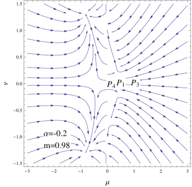
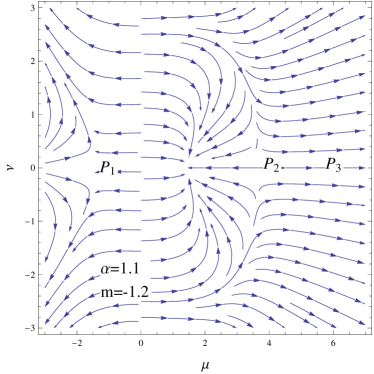
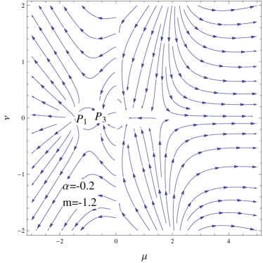
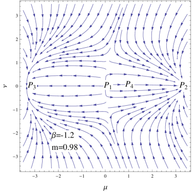
We are interested to explore the influence of physical parameters (α𝛼\alpha and m𝑚m) on the stability of cosmos coupled with scalar field. We plot the dynamical characteristics of critical points for Q=ασ˙m𝑄𝛼subscript˙𝜎𝑚Q=\alpha\dot{\sigma}_{m} in the vicinity of different values of α𝛼\alpha and m𝑚m as shown in Figure 1. We find negative eigenvalues which show the point P1subscript𝑃1P_{1} as a stable future attractor for m>0𝑚0m>0 in the physical phase space except for α=1𝛼1\alpha=1 at which the system becomes undetermined. For α,m<0𝛼𝑚0\alpha,~{}m<0, this point behaves as an unstable node.

The effective potential for the cosmic fluid is defined as

weff=1+1m+2[9+(2m+1)2(μ2+ν2)].subscript𝑤𝑒𝑓𝑓11𝑚2delimited-[]9superscript2𝑚12superscript𝜇2superscript𝜈2w_{eff}=-1+\frac{1}{m+2}[-9+(2m+1)^{2}(\mu^{2}+\nu^{2})]. (22)

We also evaluate the effective EoS parameter and deceleration parameter as

wϕsubscript𝑤italic-ϕ\displaystyle w_{\phi} =\displaystyle= 1μ2+ν2[1+1m+2{9+(2m+1)2(μ2+ν2)}],1superscript𝜇2superscript𝜈2delimited-[]11𝑚29superscript2𝑚12superscript𝜇2superscript𝜈2\displaystyle\frac{1}{\mu^{2}+\nu^{2}}\left[-1+\frac{1}{m+2}\{-9+(2m+1)^{2}(\mu^{2}+\nu^{2})\}\right], (23)
q𝑞\displaystyle q =\displaystyle= 1+1m+2[9+(2m+1)2(μ2+ν2)].11𝑚2delimited-[]9superscript2𝑚12superscript𝜇2superscript𝜈2\displaystyle-1+\frac{1}{m+2}[-9+(2m+1)^{2}(\mu^{2}+\nu^{2})]. (24)

The dynamical analysis shows accelerated expansion of the universe model for P1subscript𝑃1P_{1} as q<0𝑞0q<0.

Refer to caption
Refer to caption
Refer to caption
Refer to caption
Figure 1: Plots for phantom coupled cosmic model with Q=ασ˙m𝑄𝛼subscript˙𝜎𝑚Q=\alpha\dot{\sigma}_{m} and λ=2𝜆2\lambda=2.

For P2=(6λ6(λ2+6)2(2m+1),0)subscript𝑃26𝜆6superscript𝜆2622𝑚10P_{2}=\left(\frac{-\sqrt{6}\lambda-\sqrt{6(\lambda^{2}+6)}}{2(2m+1)},0\right), the corresponding eigenvalues are

η1subscript𝜂1\displaystyle\eta_{1} =\displaystyle= 9mm+2[13α2(1α)(2m+1){4(2m+1)2[6λ+6(λ2+6)]2+2m+13}\displaystyle\frac{9m}{m+2}\left[-1-\frac{3\alpha}{2(1-\alpha)(2m+1)}\left\{\frac{-4(2m+1)^{2}}{[\sqrt{6}\lambda+\sqrt{6(\lambda^{2}+6)}]^{2}}+\frac{2m+1}{3}\right\}\right. (25)
+\displaystyle+ 32(m+2)[6λ+6(λ2+6)]28(m+2)],\displaystyle\left.\frac{3}{2(m+2)}-\frac{[\sqrt{6}\lambda+\sqrt{6(\lambda^{2}+6)}]^{2}}{8(m+2)}\right],
η2subscript𝜂2\displaystyle\eta_{2} =\displaystyle= 3mm+2[32λ6(λ2+6)λ+6λm+2+12(m+2){9\displaystyle-\frac{3m}{m+2}\left[\sqrt{\frac{3}{2}}\lambda\frac{\sqrt{6(\lambda^{2}+6)\lambda}+\sqrt{6}\lambda}{m+2}+\frac{1}{2(m+2)}\left\{-9\right.\right. (26)
+\displaystyle+ [6(λ2+6)+6λ]24}].\displaystyle\left.\left.\frac{[\sqrt{6(\lambda^{2}+6)}+\sqrt{6}\lambda]^{2}}{4}\right\}\right].

This point shows a stable attractor with decelerated expansion for m>0𝑚0m>0. This point becomes unstable past attractor for negative values of m𝑚m. We find that α<0𝛼0\alpha<0 gives accelerated expansion while the universe undergoes decelerated expansion for α=1.1𝛼1.1\alpha=1.1 as q>0𝑞0q>0.

For P3=(3(m+2)(2α)+[3(m+2)(2α)]2+36α(1α)(m+2)2(1α)(2m+1),0)subscript𝑃33𝑚22𝛼superscriptdelimited-[]3𝑚22𝛼236𝛼1𝛼𝑚221𝛼2𝑚10P_{3}=\left(\frac{\sqrt{3(m+2)(2-\alpha)+\sqrt{[3(m+2)(2-\alpha)]^{2}+36\alpha(1-\alpha)(m+2)}}}{2(1-\alpha)(2m+1)},0\right), we have

η1subscript𝜂1\displaystyle\eta_{1} =\displaystyle= 9mm+2[α(m+2)(2α)+[(m+2)(2α)]2+4α(1α)(m+2)\displaystyle\frac{9m}{m+2}\left[\frac{\alpha}{(m+2)(2-\alpha)+\sqrt{[(m+2)(2-\alpha)]^{2}+4\alpha(1-\alpha)(m+2)}}\right.
+\displaystyle+ α22(1α)+32(m+2)+2m+12(1α)𝛼221𝛼32𝑚22𝑚121𝛼\displaystyle\left.\frac{\alpha-2}{2(1-\alpha)}+\frac{3}{2(m+2)}+\frac{2m+1}{2(1-\alpha)}\right.
×\displaystyle\times {3(m+2)(2α)+[3(m+2)(2α)]2+36α(1α)(m+2)}],\displaystyle\left.\{3(m+2)(2-\alpha)+\sqrt{[3(m+2)(2-\alpha)]^{2}+36\alpha(1-\alpha)(m+2)}\}\right],
η2subscript𝜂2\displaystyle\eta_{2} =\displaystyle= 3mm+2[92(m+2)+32λ(2m+1m+2)\displaystyle-\frac{3m}{m+2}\left[-\frac{9}{2(m+2)}+\sqrt{\frac{3}{2}}\lambda\left(\frac{2m+1}{m+2}\right)\right. (28)
×\displaystyle\times 3(m+2)(2α)+[3(m+2)(2α)]2+36α(1α)(m+2)2(1α)(2m+1)3𝑚22𝛼superscriptdelimited-[]3𝑚22𝛼236𝛼1𝛼𝑚221𝛼2𝑚1\displaystyle\left.\frac{\sqrt{3(m+2)(2-\alpha)+\sqrt{[3(m+2)(2-\alpha)]^{2}+36\alpha(1-\alpha)(m+2)}}}{2(1-\alpha)(2m+1)}\right.
+\displaystyle+ (2m+1)24(m+2)(2m+1)(1α){3(m+2)(2α)\displaystyle\left.\frac{(2m+1)^{2}}{4(m+2)(2m+1)(1-\alpha)}\{3(m+2)(2-\alpha)\right.
+\displaystyle+ [3(m+2)(2α)]2+36α(1α)(m+2)}].\displaystyle\left.\sqrt{[3(m+2)(2-\alpha)]^{2}+36\alpha(1-\alpha)(m+2)}\}\right].

For positive values of m𝑚m, this behaves as a saddle point showing decelerated expansion ultimately followed by accelerated expansion. For m<0𝑚0m<0, this point is saddle or stable showing accelerated expanding universe model corresponding to α<0𝛼0\alpha<0 or α>0𝛼0\alpha>0, respectively.
For P4=(3(m+2)(2α)[3(m+2)(2α)]2+36α(1α)(m+2)2(1α)(2m+1),0)subscript𝑃43𝑚22𝛼superscriptdelimited-[]3𝑚22𝛼236𝛼1𝛼𝑚221𝛼2𝑚10P_{4}=\left(\frac{\sqrt{3(m+2)(2-\alpha)-\sqrt{[3(m+2)(2-\alpha)]^{2}+36\alpha(1-\alpha)(m+2)}}}{2(1-\alpha)(2m+1)},0\right), we have

η1subscript𝜂1\displaystyle\eta_{1} =\displaystyle= 9mm+2[α(m+2)(2α)[(m+2)(2α)]2+4α(1α)(m+2)\displaystyle\frac{9m}{m+2}\left[\frac{\alpha}{(m+2)(2-\alpha)-\sqrt{[(m+2)(2-\alpha)]^{2}+4\alpha(1-\alpha)(m+2)}}\right.
+\displaystyle+ α22(1α)+32(m+2)+2m+12(1α)𝛼221𝛼32𝑚22𝑚121𝛼\displaystyle\left.\frac{\alpha-2}{2(1-\alpha)}+\frac{3}{2(m+2)}+\frac{2m+1}{2(1-\alpha)}\right.
×\displaystyle\times {3(m+2)(2α)[3(m+2)(2α)]2+36α(1α)(m+2)}],\displaystyle\left.\{3(m+2)(2-\alpha)-\sqrt{[3(m+2)(2-\alpha)]^{2}+36\alpha(1-\alpha)(m+2)}\}\right],
η2subscript𝜂2\displaystyle\eta_{2} =\displaystyle= 3mm+2[92(m+2)+32λ(2m+1m+2)\displaystyle-\frac{3m}{m+2}\left[-\frac{9}{2(m+2)}+\sqrt{\frac{3}{2}}\lambda\left(\frac{2m+1}{m+2}\right)\right. (30)
×\displaystyle\times 3(m+2)(2α)[3(m+2)(2α)]2+36α(1α)(m+2)2(1α)(2m+1)3𝑚22𝛼superscriptdelimited-[]3𝑚22𝛼236𝛼1𝛼𝑚221𝛼2𝑚1\displaystyle\left.\frac{\sqrt{3(m+2)(2-\alpha)-\sqrt{[3(m+2)(2-\alpha)]^{2}+36\alpha(1-\alpha)(m+2)}}}{2(1-\alpha)(2m+1)}\right.
+\displaystyle+ (2m+1)24(m+2)(2m+1)(1α){3(m+2)(2α)\displaystyle\left.\frac{(2m+1)^{2}}{4(m+2)(2m+1)(1-\alpha)}\{3(m+2)(2-\alpha)\right.
\displaystyle- [3(m+2)(2α)]2+36α(1α)(m+2)}].\displaystyle\left.\sqrt{[3(m+2)(2-\alpha)]^{2}+36\alpha(1-\alpha)(m+2)}\}\right].

This point behaves as a saddle point for all choices except for α>0𝛼0\alpha>0 and m>0𝑚0m>0 that show stable future attractor.

Table 1: Phase Space Analysis for the Phantom Coupled System with Q=ασ˙m𝑄𝛼subscript˙𝜎𝑚Q=\alpha\dot{\sigma}_{m}. Ranges of m𝑚m and α𝛼\alpha for Critical Points Stability ωϕsubscript𝜔italic-ϕ\omega_{\phi} q𝑞q Acceleration P1subscript𝑃1P_{1} m=0.98,α=1.1(α1)formulae-sequence𝑚0.98𝛼1.1𝛼1m=0.98,~{}\alpha=1.1~{}(\alpha\neq 1) Stable -6.41 -1.87 Yes m=0.98,α=0.2formulae-sequence𝑚0.98𝛼0.2m=0.98,~{}\alpha=-0.2 Stable -3.38 -0.73 Yes m=1.2,α=0.2(m2)formulae-sequence𝑚1.2𝛼0.2𝑚2m=-1.2,~{}\alpha=-0.2~{}(m\neq-2) Unstable -1.18 -0.003 Yes m=1.2,α=1.1formulae-sequence𝑚1.2𝛼1.1~{}m=-1.2,~{}\alpha=1.1 Saddle -3.92 -4.27 Yes P2subscript𝑃2P_{2} m=0.98,α=1.1(α1)formulae-sequence𝑚0.98𝛼1.1𝛼1m=0.98~{},\alpha=1.1~{}(\alpha\neq 1) Stable 1.301 1.096 No m=0.98,α=0.2formulae-sequence𝑚0.98𝛼0.2m=0.98,~{}\alpha=-0.2 Stable -1.67 -1.23 Yes m=1.2,α=0.2(m0.5,2)formulae-sequence𝑚1.2𝛼0.2𝑚0.52m=-1.2,~{}\alpha=-0.2~{}(m\neq-0.5,-2) Unstable -1.69 -1.84 Yes m=1.2,α=1.1formulae-sequence𝑚1.2𝛼1.1m=-1.2,~{}\alpha=1.1 Unstable 1.3 6.8 No P3subscript𝑃3P_{3} m=0.98,α=1.1(α1)formulae-sequence𝑚0.98𝛼1.1𝛼1m=0.98,~{}\alpha=1.1(\alpha\neq 1) Saddle 2.85 61.76 No m=0.98,α=0.2formulae-sequence𝑚0.98𝛼0.2m=0.98,~{}\alpha=-0.2 Saddle -2.306 -1.383 Yes m=1.2,α=0.2(m0.5,2)formulae-sequence𝑚1.2𝛼0.2𝑚0.52m=-1.2,~{}\alpha=-0.2~{}(m\neq-0.5,-2) Saddle -11.57 -5.56 Yes m=1.2,α=1.1formulae-sequence𝑚1.2𝛼1.1m=-1.2,~{}\alpha=1.1 Stable 2.16 46.25 No P4subscript𝑃4P_{4} m=0.98,α=1.1(α1)formulae-sequence𝑚0.98𝛼1.1𝛼1m=0.98,~{}\alpha=1.1~{}(\alpha\neq 1) Stable 1.11 0.72 No m=0.98,α=0.2formulae-sequence𝑚0.98𝛼0.2m=0.98,~{}\alpha=-0.2 Saddle -301.77 -2.49 Yes m=1.2,α=0.2(m0.5,2)formulae-sequence𝑚1.2𝛼0.2𝑚0.52m=-1.2,~{}\alpha=-0.2~{}(m\neq-0.5,-2) Saddle -194.81 -6.54 Yes m=1.2,α=1.1formulae-sequence𝑚1.2𝛼1.1m=-1.2,~{}\alpha=1.1 Saddle 1.42 8.003 No

It is mentioned here that all the points lie in accelerated expanding phase of the universe for negative values of α𝛼\alpha as q<0𝑞0q<0 and ωϕ<1subscript𝜔italic-ϕ1\omega_{\phi}<-1. We summarize the results for stability of LRS BI universe coupled with phantom energy and matter in Table 1.

3.2 Coupling Q=βσ˙ϕ𝑄𝛽subscript˙𝜎italic-ϕQ=\beta\dot{\sigma}_{\phi}

For this coupling, Eq.(13) leads to

ϕ¨Hϕ˙=3322m+1m+2λν2μ+3β1+β.¨italic-ϕ𝐻˙italic-ϕ3322𝑚1𝑚2𝜆superscript𝜈2𝜇3𝛽1𝛽\displaystyle\frac{\ddot{\phi}}{H\dot{\phi}}=-3-\sqrt{\frac{3}{2}}\frac{2m+1}{m+2}\frac{\lambda\nu^{2}}{\mu}+\frac{3\beta}{1+\beta}. (31)

Similarly, the autonomous system of equations takes the form

μsuperscript𝜇\displaystyle\mu^{\prime} =\displaystyle= 3mm+2μ[3322m+1m+2λν2μ+3β1+β12(m+2)\displaystyle\frac{3m}{m+2}\mu\left[-3-\sqrt{\frac{3}{2}}\frac{2m+1}{m+2}\frac{\lambda\nu^{2}}{\mu}+\frac{3\beta}{1+\beta}-\frac{1}{2(m+2)}\right. (32)
×\displaystyle\times {9+(2m+1)2(μ2+ν2)}],\displaystyle\left.\{-9+(2m+1)^{2}(\mu^{2}+\nu^{2})\}\right],
νsuperscript𝜈\displaystyle\nu^{\prime} =\displaystyle= 3mm+2ν[322m+1m+2μλ+12(m+2){9+(2m+1)2(μ2+ν2)}],3𝑚𝑚2𝜈delimited-[]322𝑚1𝑚2𝜇𝜆12𝑚29superscript2𝑚12superscript𝜇2superscript𝜈2\displaystyle-\frac{3m}{m+2}\nu\left[\sqrt{\frac{3}{2}}\frac{2m+1}{m+2}\mu\lambda+\frac{1}{2(m+2)}\{-9+(2m+1)^{2}(\mu^{2}+\nu^{2})\}\right],

We follow the same procedure to find the critical points. For P1=(0,0)subscript𝑃100P_{1}=(0,0), we have

η1=9m[2m+3β+7]2(m+2)2(1+β),η2=27m2(m+2)2.formulae-sequencesubscript𝜂19𝑚delimited-[]2𝑚3𝛽72superscript𝑚221𝛽subscript𝜂227𝑚2superscript𝑚22\displaystyle\eta_{1}=-\frac{9m[2m+3\beta+7]}{2(m+2)^{2}(1+\beta)},\quad\eta_{2}=\frac{27m}{2(m+2)^{2}}. (34)

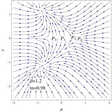
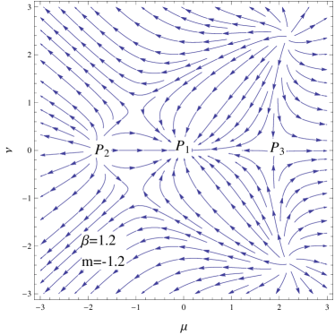
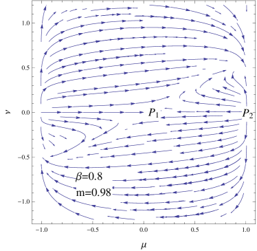
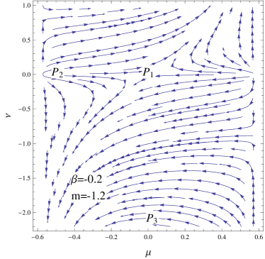
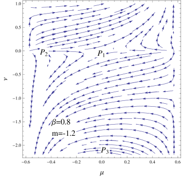
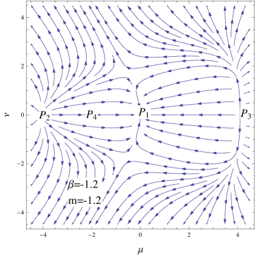
This point gives a changing behavior of critical points corresponding to different values of β𝛽\beta and m𝑚m. For β=1.2,0.8𝛽1.20.8\beta=-1.2,0.8, the point P1subscript𝑃1P_{1} is an unstable node by taking λ=2𝜆2\lambda=2 (Figure 2). For β=1𝛽1\beta=-1, the eigenvalues become undetermined, hence we neglect it. The negative value of m𝑚m gives stable future attractor. It is found that point P1subscript𝑃1P_{1} indicates accelerated expansion of cosmos since q<0𝑞0q<0 for different choices of parameters.
Refer to caption
Refer to caption
Refer to caption
Refer to caption
Figure 2: Plots for phantom coupled cosmic model with Q=βσ˙ϕ𝑄𝛽subscript˙𝜎italic-ϕQ=\beta\dot{\sigma}_{\phi} and λ=1.5𝜆1.5\lambda=1.5.

For P2=(12m+13[3β(2m+1)]1+β,0)subscript𝑃212𝑚13delimited-[]3𝛽2𝑚11𝛽0P_{2}=\left(\frac{1}{2m+1}\sqrt{\frac{3[3\beta-(2m+1)]}{1+\beta}},0\right), the eigenvalues are given by

η1subscript𝜂1\displaystyle\eta_{1} =\displaystyle= 9m(m+2)2(1+β)[3β4m5],9𝑚superscript𝑚221𝛽delimited-[]3𝛽4𝑚5\displaystyle\frac{9m}{(m+2)^{2}(1+\beta)}[3\beta-4m-5], (35)
η2subscript𝜂2\displaystyle\eta_{2} =\displaystyle= 9m(m+2)2[λ3β(2m+1)2(1+β)m+21+β].9𝑚superscript𝑚22delimited-[]𝜆3𝛽2𝑚121𝛽𝑚21𝛽\displaystyle-\frac{9m}{(m+2)^{2}}\left[\lambda\sqrt{\frac{3\beta-(2m+1)}{2(1+\beta)}}-\frac{m+2}{1+\beta}\right]. (36)

Here all values of m𝑚m and β𝛽\beta correspond to saddle or unstable points except m>0𝑚0m>0 and β<0𝛽0\beta<0 that yield stable future attractor. The universe undergoes decelerated expansion for negative values of β𝛽\beta while β>0𝛽0\beta>0 corresponds to the accelerated expansion. For P3=(12m+13[3β(2m+1)]1+β,0)subscript𝑃312𝑚13delimited-[]3𝛽2𝑚11𝛽0P_{3}=\left(-\frac{1}{2m+1}\sqrt{\frac{3[3\beta-(2m+1)]}{1+\beta}},0\right), the eigenvalues are obtained as

η1subscript𝜂1\displaystyle\eta_{1} =\displaystyle= 9m(m+2)2(1+β)[3β4m5],9𝑚superscript𝑚221𝛽delimited-[]3𝛽4𝑚5\displaystyle\frac{9m}{(m+2)^{2}(1+\beta)}[3\beta-4m-5], (37)
η2subscript𝜂2\displaystyle\eta_{2} =\displaystyle= 9m(m+2)2[λ3β(2m+1)2(1+β)+m+21+β].9𝑚superscript𝑚22delimited-[]𝜆3𝛽2𝑚121𝛽𝑚21𝛽\displaystyle\frac{9m}{(m+2)^{2}}\left[\lambda\sqrt{\frac{3\beta-(2m+1)}{2(1+\beta)}}+\frac{m+2}{1+\beta}\right]. (38)

We find that point P3subscript𝑃3P_{3} is a saddle node for all choices of β𝛽\beta and m𝑚m except for β<0𝛽0\beta<0 and m>0𝑚0m>0 at which it behaves as a stable point. This point yields decelerated expansion for negative values of β𝛽\beta. For P4=(0,±32m+1)subscript𝑃40plus-or-minus32𝑚1P_{4}=\left(0,\pm\frac{3}{2m+1}\right), the eigenvalues are

η1=9m(m+2)(1+β),η2=27m(m+2)2.formulae-sequencesubscript𝜂19𝑚𝑚21𝛽subscript𝜂227𝑚superscript𝑚22\displaystyle\eta_{1}=-\frac{9m}{(m+2)(1+\beta)},\quad\eta_{2}=-\frac{27m}{(m+2)^{2}}. (39)

This point is a saddle node for negative values of β𝛽\beta while β>0𝛽0\beta>0 corresponds to stable/unstable attractors depending on parameter m𝑚m. It is found that P4subscript𝑃4P_{4} lies in a region of accelerated expansion for all the choices of parameters. Table 2 shows the dynamical analysis for LRS BI model.

Table 2: Phase Space Analysis for the Phantom Coupled System with Q=βσ˙ϕ𝑄𝛽subscript˙𝜎italic-ϕQ=\beta\dot{\sigma}_{\phi}. Ranges of m𝑚m and β𝛽\beta for Critical Points Stability ωϕsubscript𝜔italic-ϕ\omega_{\phi} q𝑞q Acceleration P1subscript𝑃1P_{1} m=0.98,β=1.2formulae-sequence𝑚0.98𝛽1.2m=0.98,~{}\beta=1.2 Saddle Undetermined -2.51 Yes m=0.98,β=1.2,(β1)formulae-sequence𝑚0.98𝛽1.2𝛽1m=0.98,~{}\beta=-1.2,~{}(\beta\neq-1) Unstable Undetermined -2.51 Yes m=1.2,β=1.2formulae-sequence𝑚1.2𝛽1.2m=-1.2,~{}\beta=-1.2 Stable Undetermined -6.63 Yes m=1.2,β=1.2formulae-sequence𝑚1.2𝛽1.2m=-1.2,~{}\beta=1.2 Stable Undetermined -6.63 Yes P2subscript𝑃2P_{2} m=0.98,β=1.2formulae-sequence𝑚0.98𝛽1.2m=0.98,~{}\beta=1.2 Saddle -37.41 -2.36 Yes m=0.98,β=1.2,(β1)formulae-sequence𝑚0.98𝛽1.2𝛽1m=0.98,~{}\beta=-1.2,~{}(\beta\neq-1) Stable 2.58 14 No m=1.2,β=1.2,(m0.5)formulae-sequence𝑚1.2𝛽1.2𝑚0.5m=-1.2,~{}\beta=-1.2,~{}(m\neq-0.5) Saddle 1.72 14 No m=1.2,β=1.2formulae-sequence𝑚1.2𝛽1.2m=-1.2,~{}\beta=1.2 Unstable -1.07 -2.36 Yes P3subscript𝑃3P_{3} m=0.98,β=1.2formulae-sequence𝑚0.98𝛽1.2m=0.98,~{}\beta=1.2 Saddle -37.42 -2.36 Yes m=0.98,β=1.2,(β1)formulae-sequence𝑚0.98𝛽1.2𝛽1m=0.98,~{}\beta=-1.2,~{}(\beta\neq-1) Stable 2.58 14 No m=1.2,β=1.2,(m0.5)formulae-sequence𝑚1.2𝛽1.2𝑚0.5m=-1.2,~{}\beta=-1.2,~{}(m\neq-0.5) Saddle 1.72 14 No m=1.2,β=1.2formulae-sequence𝑚1.2𝛽1.2m=-1.2,~{}\beta=1.2 Saddle -1.07 -2.36 Yes P4subscript𝑃4P_{4} m=0.98,β=1.2formulae-sequence𝑚0.98𝛽1.2m=0.98,~{}\beta=1.2 Stable -0.97 -1 Yes m=0.98,β=1.2,(β1)formulae-sequence𝑚0.98𝛽1.2𝛽1m=0.98,~{}\beta=-1.2,~{}(\beta\neq-1) Saddle -0.97 -1 Yes m=1.2,β=1.2formulae-sequence𝑚1.2𝛽1.2m=-1.2,~{}\beta=-1.2 Saddle -0.217 -1 Yes m=1.2,β=1.2formulae-sequence𝑚1.2𝛽1.2m=-1.2,~{}\beta=1.2 Unstable -0.217 -1 Yes

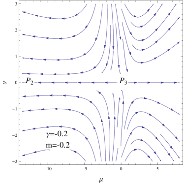
3.3 Coupling Q=γ(σ˙m+σ˙ϕ)𝑄𝛾subscript˙𝜎𝑚subscript˙𝜎italic-ϕQ=\gamma(\dot{\sigma}_{m}+\dot{\sigma}_{\phi})

In this section, we assume a combination of the form σ˙msubscript˙𝜎𝑚\dot{\sigma}_{m} and σ˙ϕsubscript˙𝜎italic-ϕ\dot{\sigma}_{\phi} for the coupling through which Eq.(13) becomes

ϕ¨Hϕ˙=3322m+1m+2λν2μ3γΩm2(1γ)μ2+3γ1+γ.¨italic-ϕ𝐻˙italic-ϕ3322𝑚1𝑚2𝜆superscript𝜈2𝜇3𝛾subscriptΩ𝑚21𝛾superscript𝜇23𝛾1𝛾\displaystyle\frac{\ddot{\phi}}{H\dot{\phi}}=-3-\sqrt{\frac{3}{2}}\frac{2m+1}{m+2}\frac{\lambda\nu^{2}}{\mu}-\frac{3\gamma\Omega_{m}}{2(1-\gamma)\mu^{2}}+\frac{3\gamma}{1+\gamma}. (40)

The evolution and conservation equations are given by

μsuperscript𝜇\displaystyle\mu^{\prime} =\displaystyle= 3mm+2μ[3322m+1m+2λν2μ3γΩm2(1γ)μ2+3γ1+γ12(m+2)\displaystyle\frac{3m}{m+2}\mu\left[-3-\sqrt{\frac{3}{2}}\frac{2m+1}{m+2}\frac{\lambda\nu^{2}}{\mu}-\frac{3\gamma\Omega_{m}}{2(1-\gamma)\mu^{2}}+\frac{3\gamma}{1+\gamma}-\frac{1}{2(m+2)}\right. (41)
×\displaystyle\times {9+(2m+1)2(μ2+ν2)}],\displaystyle\left.\{-9+(2m+1)^{2}(\mu^{2}+\nu^{2})\}\right],
νsuperscript𝜈\displaystyle\nu^{\prime} =\displaystyle= 3mm+2ν[32μλ(2m+1m+2)+12(m+2){9+(2m+1)2(μ2+ν2)}].3𝑚𝑚2𝜈delimited-[]32𝜇𝜆2𝑚1𝑚212𝑚29superscript2𝑚12superscript𝜇2superscript𝜈2\displaystyle-\frac{3m}{m+2}\nu\left[\sqrt{\frac{3}{2}}\mu\lambda\left(\frac{2m+1}{m+2}\right)+\frac{1}{2(m+2)}\{-9+(2m+1)^{2}(\mu^{2}+\nu^{2})\}\right].

For P1=(2m+1m+232λ+32λ2+(3(2m+1)m+2)2(2m+1)2/(m+2),0)subscript𝑃12𝑚1𝑚232𝜆32superscript𝜆2superscript32𝑚1𝑚22superscript2𝑚12𝑚20P_{1}=\left(\frac{-\frac{2m+1}{m+2}\sqrt{\frac{3}{2}}\lambda+\sqrt{\frac{3}{2}\lambda^{2}+\left(\frac{3(2m+1)}{m+2}\right)^{2}}}{(2m+1)^{2}/(m+2)},0\right), the corresponding eigenvalues are

η1subscript𝜂1\displaystyle\eta_{1} =\displaystyle= 9mm+2[12m2(m+2)+γ2(1γ){(2m+1)4(m+2)2{2m+1m+232λ+32λ2+(3(2m+1)m+2)2}2\displaystyle\frac{9m}{m+2}\left[\frac{1-2m}{2(m+2)}+\frac{\gamma}{2(1-\gamma)}\left\{\frac{(2m+1)^{4}}{(m+2)^{2}\left\{-\frac{2m+1}{m+2}\sqrt{\frac{3}{2}}\lambda+\sqrt{\frac{3}{2}\lambda^{2}+\left(\frac{3(2m+1)}{m+2}\right)^{2}}\right\}^{2}}\right.\right. (43)
\displaystyle- 2m+13}+γ1+γ12(m+2){2m+1m+232λ+32λ2+(3(2m+1)m+2)2(2m+1)2/(m+2)}2],\displaystyle\left.\left.\frac{2m+1}{3}\right\}+\frac{\gamma}{1+\gamma}-\frac{1}{2(m+2)}\left\{\frac{-\frac{2m+1}{m+2}\sqrt{\frac{3}{2}}\lambda+\sqrt{\frac{3}{2}\lambda^{2}+\left(\frac{3(2m+1)}{m+2}\right)^{2}}}{(2m+1)^{2}/(m+2)}\right\}^{2}\right],
η2subscript𝜂2\displaystyle\eta_{2} =\displaystyle= 3mm+2[32λ{2m+1m+232λ+32λ2+(3(2m+1)m+2)2(2m+1)}+12(m+2)\displaystyle-\frac{3m}{m+2}\left[\sqrt{\frac{3}{2}}\lambda\left\{\frac{-\frac{2m+1}{m+2}\sqrt{\frac{3}{2}}\lambda+\sqrt{\frac{3}{2}\lambda^{2}+\left(\frac{3(2m+1)}{m+2}\right)^{2}}}{(2m+1)}\right\}+\frac{1}{2(m+2)}\right.
×\displaystyle\times {9+(m+22m+1)2[(2m+1m+2)32λ+32λ2+(3(2m+1)m+2)2]2}].\displaystyle\left.\left\{-9+\left(\frac{m+2}{2m+1}\right)^{2}\left[-\left(\frac{2m+1}{m+2}\right)\sqrt{\frac{3}{2}}\lambda+\sqrt{\frac{3}{2}\lambda^{2}+\left(\frac{3(2m+1)}{m+2}\right)^{2}}\right]^{2}\right\}\right].

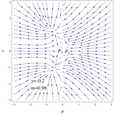
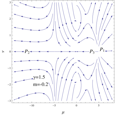
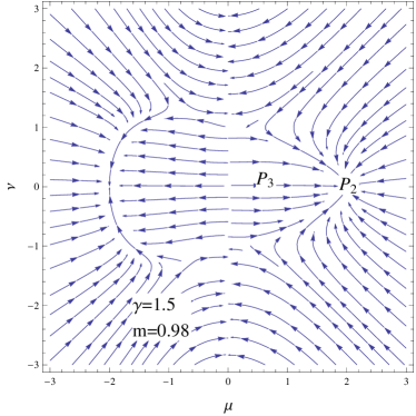
In this case, we examine unstable nodes for m<0𝑚0m<0 by varying γ𝛾\gamma that shows decelerated expanding universe except for m=0.5,2𝑚0.52m=-0.5,-2 (Figure 3). On the other hand, the positive values of m𝑚m give accelerated expansion of the universe.
Refer to caption
Refer to caption
Refer to caption
Refer to caption
Figure 3: Plots for phantom coupled cosmic model with Q=γ(σ˙m+σ˙ϕ)𝑄𝛾subscript˙𝜎𝑚subscript˙𝜎italic-ϕQ=\gamma(\dot{\sigma}_{m}+\dot{\sigma}_{\phi}) and λ=1.5𝜆1.5\lambda=1.5.

For P2=(2m+1m+232λ32λ2+(3(2m+1)m+2)2(2m+1)2/(m+2),0)subscript𝑃22𝑚1𝑚232𝜆32superscript𝜆2superscript32𝑚1𝑚22superscript2𝑚12𝑚20P_{2}=\left(\frac{-\frac{2m+1}{m+2}\sqrt{\frac{3}{2}}\lambda-\sqrt{\frac{3}{2}\lambda^{2}+\left(\frac{3(2m+1)}{m+2}\right)^{2}}}{(2m+1)^{2}/(m+2)},0\right), the corresponding eigenvalues are given as

η1subscript𝜂1\displaystyle\eta_{1} =\displaystyle= 9mm+2[12m2(m+2)+γ2(1γ){(2m+1)4(m+2)2{2m+1m+232λ32λ2+(3(2m+1)m+2)2}2\displaystyle\frac{9m}{m+2}\left[\frac{1-2m}{2(m+2)}+\frac{\gamma}{2(1-\gamma)}\left\{\frac{(2m+1)^{4}}{(m+2)^{2}\left\{-\frac{2m+1}{m+2}\sqrt{\frac{3}{2}}\lambda-\sqrt{\frac{3}{2}\lambda^{2}+\left(\frac{3(2m+1)}{m+2}\right)^{2}}\right\}^{2}}\right.\right. (45)
\displaystyle- 2m+13}+γ1+γ12(m+2){2m+1m+232λ32λ2+(3(2m+1)m+2)2(2m+1)2/(m+2)}2],\displaystyle\left.\left.\frac{2m+1}{3}\right\}+\frac{\gamma}{1+\gamma}-\frac{1}{2(m+2)}\left\{\frac{-\frac{2m+1}{m+2}\sqrt{\frac{3}{2}}\lambda-\sqrt{\frac{3}{2}\lambda^{2}+\left(\frac{3(2m+1)}{m+2}\right)^{2}}}{(2m+1)^{2}/(m+2)}\right\}^{2}\right],
η2subscript𝜂2\displaystyle\eta_{2} =\displaystyle= 3mm+2[32λ{2m+1m+232λ32λ2+(3(2m+1)m+2)2(2m+1)}\displaystyle-\frac{3m}{m+2}\left[\sqrt{\frac{3}{2}}\lambda\left\{\frac{-\frac{2m+1}{m+2}\sqrt{\frac{3}{2}}\lambda-\sqrt{\frac{3}{2}\lambda^{2}+\left(\frac{3(2m+1)}{m+2}\right)^{2}}}{(2m+1)}\right\}\right.
+\displaystyle+ 1m+2{9+(m+2)2m+2[(2m+1m+2)32λ32λ2+(3(2m+1)m+2)2]2}].\displaystyle\left.\frac{1}{m+2}\left\{-9+\frac{(m+2)^{2}}{m+2}\left[-\left(\frac{2m+1}{m+2}\right)\frac{3}{2}\lambda-\sqrt{\frac{3}{2}\lambda^{2}+\left(\frac{3(2m+1)}{m+2}\right)^{2}}\right]^{2}\right\}\right].

This point corresponds to either stable or unstable nodes for m>0𝑚0m>0 or m<0𝑚0m<0, respectively. It is found that P2subscript𝑃2P_{2} lies in the matter dominated phase for all choices of the parameters. For
P3=(m+2(2m+1)γ(2m+1)2(1γ)31+γ+92(m+2)+ξ,0)subscript𝑃3𝑚22𝑚1𝛾2𝑚121𝛾31𝛾92𝑚2𝜉0P_{3}=\left(\frac{\sqrt{m+2}}{(2m+1)}\sqrt{\frac{\gamma(2m+1)}{2(1-\gamma)}-\frac{3}{1+\gamma}+\frac{9}{2(m+2)}+\xi},0\right), the eigenvalues are

η1subscript𝜂1\displaystyle\eta_{1} =\displaystyle= 9mm+2[2(2m+1)2γ(1+γ)2γ(m+2)+4(m+1)(1γ2)(ξ3)+9+12(1+γ)\displaystyle\frac{9m}{m+2}\left[\frac{2(2m+1)^{2}\gamma(1+\gamma)}{2\gamma(m+2)+4(m+1)(1-\gamma^{2})(\xi-3)+9}+\frac{1}{2(1+\gamma)}\right. (47)
+\displaystyle+ 5γ(2m+1)12(1γ)34(m+2)ξ2],\displaystyle\left.\frac{5\gamma(2m+1)}{12(1-\gamma)}-\frac{3}{4(m+2)}-\frac{\xi}{2}\right],
η2subscript𝜂2\displaystyle\eta_{2} =\displaystyle= 3mm+2[32(m+2)(γ(2m+1)2(1γ)31+γ+92(m+2)+ξ)\displaystyle-\frac{3m}{m+2}\left[\sqrt{\frac{3}{2(m+2)}\left(\frac{\gamma(2m+1)}{2(1-\gamma)}-\frac{3}{1+\gamma}+\frac{9}{2(m+2)}+\xi\right)}\right.
+\displaystyle+ 12(m+2){9+(m+2)(γ(2m+1)2(1γ)31+γ+92(m+2)+ξ)}],\displaystyle\left.\frac{1}{2(m+2)}\left\{-9+(m+2)\left(\frac{\gamma(2m+1)}{2(1-\gamma)}-\frac{3}{1+\gamma}+\frac{9}{2(m+2)}+\xi\right)\right\}\right],

where

ξ𝜉\displaystyle\xi =\displaystyle= 31+γγ(2m+1)2(1γ)92(m+2)3(2m+1)2γ(m+2)(1γ).31𝛾𝛾2𝑚121𝛾92𝑚23superscript2𝑚12𝛾𝑚21𝛾\displaystyle\sqrt{\frac{3}{1+\gamma}-\frac{\gamma(2m+1)}{2(1-\gamma)}-\frac{9}{2(m+2)}-\frac{3(2m+1)^{2}\gamma}{(m+2)(1-\gamma)}}.

Table 3: Phase Space Analysis for Q=γ(σ˙m+σ˙ϕ)𝑄𝛾subscript˙𝜎𝑚subscript˙𝜎italic-ϕQ=\gamma(\dot{\sigma}_{m}+\dot{\sigma}_{\phi}). Ranges of m𝑚m and γ𝛾\gamma for Critical Points Stability ωϕsubscript𝜔italic-ϕ\omega_{\phi} q𝑞q Acceleration P1subscript𝑃1P_{1} m=0.98,γ=1.5,(γ1)formulae-sequence𝑚0.98𝛾1.5𝛾1m=0.98,~{}\gamma=1.5,~{}(\gamma\neq 1) Stable -14.18 -2.16 Yes m=0.98,γ=0.2,(γ1)formulae-sequence𝑚0.98𝛾0.2𝛾1m=0.98,~{}\gamma=-0.2,~{}(\gamma\neq-1) Saddle -14.18 -2.16 Yes m=0.2,γ=0.2,(m0.5,2)formulae-sequence𝑚0.2𝛾0.2𝑚0.52m=-0.2,~{}\gamma=-0.2,~{}(m\neq-0.5,-2) Unstable 0.128 4.86 No m=0.2,γ=1.5formulae-sequence𝑚0.2𝛾1.5m=-0.2,~{}\gamma=1.5 Unstable 0.128 4.86 No P2subscript𝑃2P_{2} m=0.98,γ=1.5,(γ1)formulae-sequence𝑚0.98𝛾1.5𝛾1m=0.98,~{}\gamma=1.5,~{}(\gamma\neq 1) Stable 2.06 4.22 No m=0.98,γ=0.2,(γ1)formulae-sequence𝑚0.98𝛾0.2𝛾1m=0.98,~{}\gamma=-0.2,~{}(\gamma\neq-1) Stable 2.06 4.22 No m=0.2,γ=0.2,(m0.5,2)formulae-sequence𝑚0.2𝛾0.2𝑚0.52m=-0.2,~{}\gamma=-0.2,~{}(m\neq-0.5,-2) Unstable 0.179 26.46 No m=0.2,γ=1.5formulae-sequence𝑚0.2𝛾1.5m=-0.2,~{}\gamma=1.5 Unstable 0.179 26.46 No P3subscript𝑃3P_{3} m=0.98,γ=1.5,(γ1)formulae-sequence𝑚0.98𝛾1.5𝛾1m=0.98,~{}\gamma=1.5,~{}(\gamma\neq 1) Saddle 57.94 -2.62 Yes m=0.98,γ=0.2,(γ1)formulae-sequence𝑚0.98𝛾0.2𝛾1m=0.98,~{}\gamma=-0.2,~{}(\gamma\neq-1) Saddle 57.94 -2.62 Yes m=0.2,γ=0.2,(m2)formulae-sequence𝑚0.2𝛾0.2𝑚2m=-0.2,~{}\gamma=-0.2,~{}(m\neq-2) Saddle -1.504 -3.503 Yes m=0.2,γ=1.5formulae-sequence𝑚0.2𝛾1.5m=-0.2,~{}\gamma=1.5 Saddle -1.504 -3.503 Yes

The behavior of eigenvalues as well as trajectories indicate that point P3subscript𝑃3P_{3} is a saddle node for all choices of the parameters. The summary of the above results is provided in Table 3.

4 Coupled Tachyon Dynamics

Now we study the evolution of LRS BI universe by considering tachyon coupled cosmic fluid. The conservation equations are

σ˙m+3(σm+pm)Hsubscript˙𝜎𝑚3subscript𝜎𝑚subscript𝑝𝑚𝐻\displaystyle\dot{\sigma}_{m}+3(\sigma_{m}+p_{m})H =\displaystyle= Q,𝑄\displaystyle Q, (50)
σ˙ϕ+3(σϕ+pϕ)Hsubscript˙𝜎italic-ϕ3subscript𝜎italic-ϕsubscript𝑝italic-ϕ𝐻\displaystyle\dot{\sigma}_{\phi}+3(\sigma_{\phi}+p_{\phi})H =\displaystyle= Q,𝑄\displaystyle-Q, (51)

where σϕ=V(ϕ)1ϕ˙2subscript𝜎italic-ϕ𝑉italic-ϕ1superscript˙italic-ϕ2\sigma_{\phi}=\frac{V(\phi)}{\sqrt{1-\dot{\phi}^{2}}} and pϕ=V(ϕ)1ϕ˙2subscript𝑝italic-ϕ𝑉italic-ϕ1superscript˙italic-ϕ2p_{\phi}=-V(\phi)\sqrt{1-\dot{\phi}^{2}}. In this case, the evolution equations take the form

H2superscript𝐻2\displaystyle H^{2} =\displaystyle= (m+2)29(2m+1)[V(ϕ)1ϕ˙2+σm],superscript𝑚2292𝑚1delimited-[]𝑉italic-ϕ1superscript˙italic-ϕ2subscript𝜎𝑚\displaystyle\frac{(m+2)^{2}}{9(2m+1)}\left[\frac{V(\phi)}{\sqrt{1-\dot{\phi}^{2}}}+\sigma_{m}\right], (52)
ϕ¨1ϕ˙2¨italic-ϕ1superscript˙italic-ϕ2\displaystyle\frac{\ddot{\phi}}{1-\dot{\phi}^{2}} =\displaystyle= [3Hϕ˙+V(ϕ)V(ϕ)+Q1ϕ˙2V(ϕ)ϕ˙].delimited-[]3𝐻˙italic-ϕsuperscript𝑉italic-ϕ𝑉italic-ϕ𝑄1superscript˙italic-ϕ2𝑉italic-ϕ˙italic-ϕ\displaystyle-\left[3H\dot{\phi}+\frac{V^{\prime}(\phi)}{V(\phi)}+\frac{Q\sqrt{1-\dot{\phi}^{2}}}{V(\phi)\dot{\phi}}\right]. (53)

Here we define the following dimensionless quantities

μ=(m+2)ϕ˙2m+1,ν=(m+2)V3(2m+1)H,λ=VVV,formulae-sequence𝜇𝑚2˙italic-ϕ2𝑚1formulae-sequence𝜈𝑚2𝑉32𝑚1𝐻𝜆superscript𝑉𝑉𝑉\displaystyle\mu=\frac{(m+2)\dot{\phi}}{2m+1},\quad\nu=\frac{(m+2)\sqrt{V}}{\sqrt{3}(2m+1)H},\quad\lambda=-\frac{V^{\prime}}{V\sqrt{V}}, (54)

such that the dynamical system yields

μsuperscript𝜇\displaystyle\mu^{\prime} =\displaystyle= 3m2m+1ϕ¨μHϕ˙,3𝑚2𝑚1¨italic-ϕ𝜇𝐻˙italic-ϕ\displaystyle\frac{3m}{2m+1}\frac{\ddot{\phi}\mu}{H\dot{\phi}}, (55)
νsuperscript𝜈\displaystyle\nu^{\prime} =\displaystyle= 33m(2m+1)2λμν22(m+2)33mνm+2H˙H2.33𝑚superscript2𝑚12𝜆𝜇superscript𝜈22superscript𝑚233𝑚𝜈𝑚2˙𝐻superscript𝐻2\displaystyle-\frac{3\sqrt{3}m(2m+1)^{2}\lambda\mu\nu^{2}}{2(m+2)^{3}}-\frac{3m\nu}{m+2}\frac{\dot{H}}{H^{2}}. (56)

We consider inverse square potential with constant parameter λ𝜆\lambda. In this case, we take the only coupling Q=βσ˙ϕ𝑄𝛽subscript˙𝜎italic-ϕQ=\beta\dot{\sigma}_{\phi} through which Eqs.(52) and (53) lead to

H˙H2˙𝐻superscript𝐻2\displaystyle\frac{\dot{H}}{H^{2}} =\displaystyle= (2m+1)22(m+2)ν21(2m+1m+2)2μ292(m+2),superscript2𝑚122𝑚2superscript𝜈21superscript2𝑚1𝑚22superscript𝜇292𝑚2\displaystyle\frac{(2m+1)^{2}}{2(m+2)}\nu^{2}\sqrt{1-\left(\frac{2m+1}{m+2}\right)^{2}\mu^{2}}-\frac{9}{2(m+2)}, (57)
ϕ¨ϕ˙H¨italic-ϕ˙italic-ϕ𝐻\displaystyle\frac{\ddot{\phi}}{\dot{\phi}H} =\displaystyle= [1(2m+1m+2)2μ2][3νλμ+3β1+β3].delimited-[]1superscript2𝑚1𝑚22superscript𝜇2delimited-[]3𝜈𝜆𝜇3𝛽1𝛽3\displaystyle\left[1-\left(\frac{2m+1}{m+2}\right)^{2}\mu^{2}\right]\left[\frac{\sqrt{3}\nu\lambda}{\mu}+\frac{3\beta}{1+\beta}-3\right]. (58)

The effective EoS and deceleration parameters can be written as

weffsubscript𝑤𝑒𝑓𝑓\displaystyle w_{eff} =\displaystyle= 113(m+2)[(2m+1)2ν21(2m+1m+2)2μ29],113𝑚2delimited-[]superscript2𝑚12superscript𝜈21superscript2𝑚1𝑚22superscript𝜇29\displaystyle-1-\frac{1}{3(m+2)}\left[(2m+1)^{2}\nu^{2}\sqrt{1-\left(\frac{2m+1}{m+2}\right)^{2}\mu^{2}}-9\right], (59)
q𝑞\displaystyle q =\displaystyle= 112(m+2)[(2m+1)2ν21(2m+1m+2)2μ29].112𝑚2delimited-[]superscript2𝑚12superscript𝜈21superscript2𝑚1𝑚22superscript𝜇29\displaystyle-1-\frac{1}{2(m+2)}\left[(2m+1)^{2}\nu^{2}\sqrt{1-\left(\frac{2m+1}{m+2}\right)^{2}\mu^{2}}-9\right]. (60)
Refer to caption
Refer to caption
Refer to caption
Refer to caption
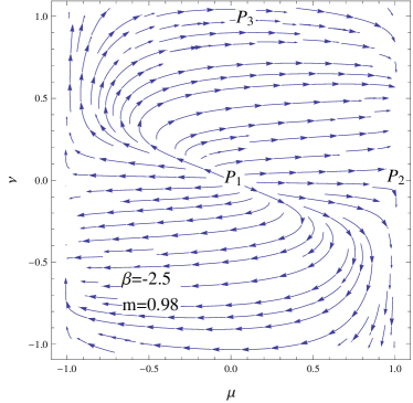
Figure 4: Plots for tachyon coupled cosmic model with Q=βσ˙ϕ𝑄𝛽subscript˙𝜎italic-ϕQ=\beta\dot{\sigma}_{\phi} and λ=2𝜆2\lambda=2.

For P1=(0,0)subscript𝑃100P_{1}=(0,0), we find the eigenvalues as

η1=9m(2m+1)(1+β),η2=27m2(m+2)2.formulae-sequencesubscript𝜂19𝑚2𝑚11𝛽subscript𝜂227𝑚2superscript𝑚22\displaystyle\eta_{1}=-\frac{9m}{(2m+1)(1+\beta)},\quad\eta_{2}=\frac{27m}{2(m+2)^{2}}. (61)

We find that point P1subscript𝑃1P_{1} is saddle/unstable for m>𝑚absentm> which becomes stable for negative values of m𝑚m (m0.5,β1formulae-sequence𝑚0.5𝛽1m\neq-0.5,\beta\neq-1) undergoing accelerated expansion as q<0𝑞0q<0 (Figure 4). We provide the obtained results in Table 4.

Table 4: Phase Space Analysis of Tachyon Coupled System with Q=βσ˙ϕ𝑄𝛽subscript˙𝜎italic-ϕQ=\beta\dot{\sigma}_{\phi}. Ranges of m𝑚m and β𝛽\beta for Critical Points Stability ωϕsubscript𝜔italic-ϕ\omega_{\phi} q𝑞q Acceleration P1subscript𝑃1P_{1} m=0.98,β=0.8formulae-sequence𝑚0.98𝛽0.8m=0.98,~{}\beta=0.8 Saddle -2.006 -2.51 Yes m=0.98,β=0.2,(β1)formulae-sequence𝑚0.98𝛽0.2𝛽1m=0.98,~{}\beta=-0.2,(~{}\beta\neq-1) Unstable -2.006 -2.51 Yes m=1.2,β=0.2,(m0.5)formulae-sequence𝑚1.2𝛽0.2𝑚0.5m=-1.2,~{}\beta=-0.2,~{}(m\neq-0.5) Stable -4.75 -6.625 Yes m=1.2,β=0.8formulae-sequence𝑚1.2𝛽0.8m=-1.2,~{}\beta=0.8 Stable -4.75 -6.625 Yes P2 m=0.98,β=0.8formulae-sequence𝑚0.98𝛽0.8m=0.98,~{}\beta=0.8 Unstable -2.006 -2.51 Yes m=0.98,β=0.2,(β1)formulae-sequence𝑚0.98𝛽0.2𝛽1m=0.98,~{}\beta=-0.2,~{}(\beta\neq-1) Saddle -2.006 -2.51 Yes m=1.2,β=0.2,(m0.5)formulae-sequence𝑚1.2𝛽0.2𝑚0.5m=-1.2,~{}\beta=-0.2,~{}(m\neq-0.5) Saddle -4.75 -6.625 Yes m=1.2,β=0.8formulae-sequence𝑚1.2𝛽0.8m=-1.2,~{}\beta=0.8 Saddle -4.75 -6.625 Yes P3 m=0.98,β=0.8formulae-sequence𝑚0.98𝛽0.8m=0.98,~{}\beta=0.8 Stable -1 -1 Yes m=0.98,β=0.2,(β1)formulae-sequence𝑚0.98𝛽0.2𝛽1m=0.98,~{}\beta=-0.2,~{}(\beta\neq-1) Saddle -1 -1 Yes m=1.2,β=0.2,(m0.5)formulae-sequence𝑚1.2𝛽0.2𝑚0.5m=-1.2,~{}\beta=-0.2,~{}(m\neq-0.5) Saddle -1 -1 Yes m=1.2,β=0.8formulae-sequence𝑚1.2𝛽0.8m=-1.2,~{}\beta=0.8 Saddle -1 -1 Yes

For P2=(±m+22m+1,0)subscript𝑃2plus-or-minus𝑚22𝑚10P_{2}=\left(\pm\frac{m+2}{2m+1},0\right), the eigenvalues become

η1=18m(2m+1)(1+β),η2=27m2(m+2)2,formulae-sequencesubscript𝜂118𝑚2𝑚11𝛽subscript𝜂227𝑚2superscript𝑚22\displaystyle\eta_{1}=\frac{18m}{(2m+1)(1+\beta)},\quad\eta_{2}=\frac{27m}{2(m+2)^{2}}, (62)

which correspond to unstable nodes for m,β>0𝑚𝛽0m,\beta>0 lying in accelerated expanding phase of the universe model. We have saddle nodes for the remaining choices of parameters m𝑚m and β𝛽\beta. The cosmic portrait indicates accelerated expansion phase of the universe for all choices of the parameters. When P3=(0,±32m+1)subscript𝑃30plus-or-minus32𝑚1P_{3}=\left(0,\pm\frac{3}{2m+1}\right), the eigenvalues yield

η1=9m(2m+1)(1+β),η2=27m(m+2)2.formulae-sequencesubscript𝜂19𝑚2𝑚11𝛽subscript𝜂227𝑚superscript𝑚22\displaystyle\eta_{1}=-\frac{9m}{(2m+1)(1+\beta)},\quad\eta_{2}=-\frac{27m}{(m+2)^{2}}. (63)

This point is a stable future attractor for β>0𝛽0\beta>0 and m>0𝑚0m>0 undergoing accelerated expansion of the cosmic model. We find that the respective point corresponds to saddle nodes for all other choices of parameters except at m=0.5,β1=m=-0.5,\beta-1=. This point indicates de Sitter (q=1𝑞1q=-1, weff=1subscript𝑤𝑒𝑓𝑓1w_{eff}=-1) phase of cosmos.

5 Power-Law Scale Factor

Here we explore the power-law behavior of the scale factor by applying some assumptions to both the phantom and tachyon coupled fields. In this context, Eq.(12) becomes

Θ˙=16(m+2)[9+(2m+1)2(μ2+ν2)]Θ2,˙Θ16𝑚2delimited-[]9superscript2𝑚12superscript𝜇2superscript𝜈2superscriptΘ2\dot{\Theta}=\frac{1}{6(m+2)}[-9+(2m+1)^{2}(\mu^{2}+\nu^{2})]\Theta^{2}, (64)

where Θ=3HΘ3𝐻\Theta=3H is the expansion scalar. For Θ0Θ0\Theta\neq 0, we formulate power-law scale factor only if 9+(2m+1)2(μ2+ν2)09superscript2𝑚12superscript𝜇2superscript𝜈20-9+(2m+1)^{2}(\mu^{2}+\nu^{2})\neq 0. We obtain the respective generic critical point by solving Θ=a˙a+2b˙bΘ˙𝑎𝑎2˙𝑏𝑏\Theta=\frac{\dot{a}}{a}+\frac{2\dot{b}}{b} for a(t)𝑎𝑡a(t) and b(t)𝑏𝑡b(t) as

b(m+2)=b0(m+2)(tt0)6(m+2)9+(2m+1)2(μ2+ν2).superscript𝑏𝑚2superscriptsubscript𝑏0𝑚2superscript𝑡subscript𝑡06𝑚29superscript2𝑚12superscript𝜇2superscript𝜈2b^{(m+2)}=b_{0}^{(m+2)}(t-t_{0})^{\frac{-6(m+2)}{-9+(2m+1)^{2}(\mu^{2}+\nu^{2})}}. (65)

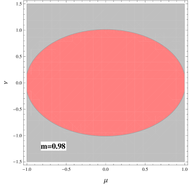
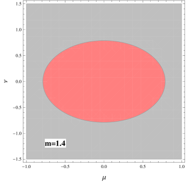
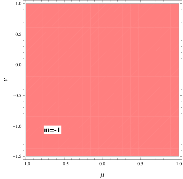
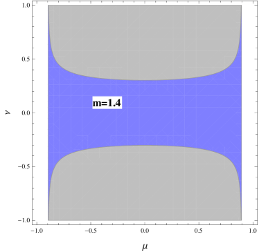
It is noticed that behavior of the term ``9+(2m+1)2(μ2+ν2)"``9superscript2𝑚12superscript𝜇2superscript𝜈2"``-9+(2m+1)^{2}(\mu^{2}+\nu^{2})" is quite important to assess different cosmological phases. It shows exponential cosmic expansion for 9+(2m+1)2(μ2+ν2)=09superscript2𝑚12superscript𝜇2superscript𝜈20-9+(2m+1)^{2}(\mu^{2}+\nu^{2})=0 while 9+(2m+1)2(μ2+ν2)0greater-than-or-less-than9superscript2𝑚12superscript𝜇2superscript𝜈20-9+(2m+1)^{2}(\mu^{2}+\nu^{2})\gtrless 0 gives accelerated cosmic expansion or contraction, respectively. Figure 5 depicts different states for power-law scale factor, where red and gray regions show contraction and accelerated expansion of cosmic model, respectively. It is found that decelerated expansion tends to increase by increasing m𝑚m whereas m<0𝑚0m<0 undergoes decelerated expansion.

Refer to caption
Refer to caption
Refer to caption
Figure 5: Plots for power-law scale factor coupled with phantom fluid. Blue and gray zones represent contraction and accelerated expansion of cosmos, respectively.

For tachyon coupled fluid, Eq.(57) becomes

Θ˙=16(m+2)[(2m+1)2ν21(2m+1m+2)2μ292(m+2)]Θ2.˙Θ16𝑚2delimited-[]superscript2𝑚12superscript𝜈21superscript2𝑚1𝑚22superscript𝜇292𝑚2superscriptΘ2\dot{\Theta}=\frac{1}{6(m+2)}\left[(2m+1)^{2}\nu^{2}\sqrt{1-\left(\frac{2m+1}{m+2}\right)^{2}\mu^{2}}-\frac{9}{2(m+2)}\right]\Theta^{2}. (66)

For Θ0Θ0\Theta\neq 0, we again find power-law scale factor if (2m+1)2ν21(2m+1m+2)2μ292(m+2)0superscript2𝑚12superscript𝜈21superscript2𝑚1𝑚22superscript𝜇292𝑚20(2m+1)^{2}\nu^{2}\sqrt{1-\left(\frac{2m+1}{m+2}\right)^{2}\mu^{2}}-\frac{9}{2(m+2)}\neq 0. The generic critical point is obtained through Θ=a˙a+2b˙bΘ˙𝑎𝑎2˙𝑏𝑏\Theta=\frac{\dot{a}}{a}+\frac{2\dot{b}}{b} as

b(m+2)=b0(m+2)(tt0)6(m+2)(2m+1)2ν21(2m+1m+2)2μ292(m+2).superscript𝑏𝑚2superscriptsubscript𝑏0𝑚2superscript𝑡subscript𝑡06𝑚2superscript2𝑚12superscript𝜈21superscript2𝑚1𝑚22superscript𝜇292𝑚2b^{(m+2)}=b_{0}^{(m+2)}(t-t_{0})^{\frac{-6(m+2)}{(2m+1)^{2}\nu^{2}\sqrt{1-\left(\frac{2m+1}{m+2}\right)^{2}\mu^{2}}-\frac{9}{2(m+2)}}}. (67)

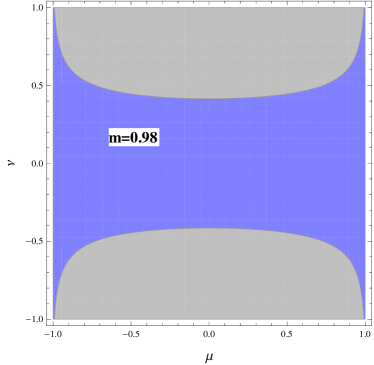
We examine various cosmological states according to (2m+1)2ν21(2m+1m+2)2μ292(m+2)0greater-than-or-less-thansuperscript2𝑚12superscript𝜈21superscript2𝑚1𝑚22superscript𝜇292𝑚20(2m+1)^{2}\nu^{2}\sqrt{1-\left(\frac{2m+1}{m+2}\right)^{2}\mu^{2}}-\frac{9}{2(m+2)}\gtrless 0. Figure 6 corresponds to the different cosmological phases, where blue and gray zones indicate contraction as well as accelerated expansion of cosmos, respectively. It is found that the region for decelerated expansion decreases by increasing m𝑚m whereas m<0𝑚0m<0 corresponds to contraction of the cosmic model (Figure 6).
Refer to caption
Refer to caption
Refer to caption
Figure 6: Plots of qualitative phase space analysis for power-law scale factor with tachyon coupled matter.

6 Summary

This work is devoted to discuss stability of LRS BI universe model by taking scalar field coupled fluid. An autonomous system of equations has been developed by introducing various dimensionless parameters. We have obtained the corresponding critical points with different choices of the parameters. The eigenvalues have been formulated which characterize the obtained critical points. We summarize the results of the dynamical analysis as follows.

Firstly, we have studied stability of the universe model dominated by the coupling of phantom energy and DM for different values of m𝑚m (Figures 1-3). We have considered three different linear combinations for the coupling parameter. For Q=ασ˙m𝑄𝛼subscript˙𝜎𝑚Q=\alpha\dot{\sigma}_{m} and (P1)subscript𝑃1(P_{1}), we have observed stable DE dominated state with m>0𝑚0m>0 and different choices of α𝛼\alpha (Figure 1). This analysis indicates a deceleration phase eventually followed by accelerated expansion of the cosmos for point P3subscript𝑃3P_{3}. It is observed that point P2subscript𝑃2P_{2} lies in non-accelerating phase of the universe as q>0𝑞0q>0 for α>0𝛼0\alpha>0 which may alleviate coincidence problem as compared to [25, 28]. For m>0𝑚0m>0, all the points show stable future attractors except P3subscript𝑃3P_{3} and P4subscript𝑃4P_{4} which shows saddle nodes depending on the choices of α𝛼\alpha.

For Q=βσ˙ϕ𝑄𝛽subscript˙𝜎italic-ϕQ=\beta\dot{\sigma}_{\phi}, all the eigenvalues and trajectories show saddle nodes for positive values of m,β𝑚𝛽m,\beta (except P4subscript𝑃4P_{4}) which become stable/unstable for m<0𝑚0m<0 corresponding to different choices of β𝛽\beta (Figure 2). It is noted that P1subscript𝑃1P_{1} and P4subscript𝑃4P_{4} undergo accelerated expansion for all choices of the parameters. For the coupling Q=γ(σ˙m+σ˙ϕ)𝑄𝛾subscript˙𝜎𝑚subscript˙𝜎italic-ϕQ=\gamma(\dot{\sigma}_{m}+\dot{\sigma}_{\phi}), we have found P1subscript𝑃1P_{1} as stable attractor for positive values of m𝑚m showing accelerated cosmic expansion. When m<0𝑚0m<0, unstable node is observed for both P1subscript𝑃1P_{1} and P2subscript𝑃2P_{2} undergoing decelerated expansion (Figure 3). In this case, point P3subscript𝑃3P_{3} shows saddle node in accelerating phases. For the coupling Q=βσ˙ϕ𝑄𝛽subscript˙𝜎italic-ϕQ=\beta\dot{\sigma}_{\phi}, P3subscript𝑃3P_{3} is the only point that indicates accelerated expanding universe for all the chosen values of parameters.

Secondly, we have discussed dynamics of the universe model by considering tachyon coupled field. In this case, we consider Q=βσ˙ϕ𝑄𝛽subscript˙𝜎italic-ϕQ=\beta\dot{\sigma}_{\phi} only. The cosmic portrait indicates accelerated expansion of the universe model (Figure 4). For m>0𝑚0m>0, points P1subscript𝑃1P_{1} and P2subscript𝑃2P_{2} behave as unstable/saddle nodes whereas P3subscript𝑃3P_{3} provides stable future attractor in accelerated expansion scenario. For m<0𝑚0m<0, the point P1subscript𝑃1P_{1} is stable showing accelerated expansion of cosmos while the remaining points act as saddle nodes that correspond to de Sitter cosmic phase. We conclude that tachyon coupled field yields an era of accelerated expansion for all choices of parameters.

Finally, we have investigated the characteristics of power-law scale factor by varying m𝑚m. It indicates various phases of evolution (accelerated or exponential expansion) for the respective cosmic model as shown (Figures 5 and 6). In case of phantom coupled matter, the region of decelerated expansion increases by increasing m𝑚m while m<0𝑚0m<0 corresponds to deceleration phase only. For tachyon coupled field, the expansion rate increases by increasing m𝑚m which directly affects the contraction rate such that blue region gets smaller. Also, the negative values of parameter m𝑚m shows only decelerated expansion of the cosmic model.

References

  • [1] A. G. Riess et al, Astron. J., 116(3): 1009 (1998) doi:10.1086/300499 arXiv:astro-ph/9805201
  • [2] S. J. Perlmutter et al, Astrophys. J., 517(2): 565 (1999) doi:10.1086/307221 arXiv:astro-ph/9812133
  • [3] C. L. Bennett et al, Astrophys. J. Suppl., 148: 1 (2003) doi:10.1086/377253 arXiv:astro-ph/0302207
  • [4] R. R. Caldwell, R. Dave and P. J. Steinhardt, Phys. Rev. Lett., 80: 1582 (1998) doi:10.1103/PhysRevLett.80.1582 arXiv:astro-ph/9708069
  • [5] T. Chiba, T. Okabe and M. Yamaguchi, Phys. Rev. D, 62: 023511 (2000) doi: 10.1103/PhysRevD.62.023511 arXiv:astro-ph/9912463
  • [6] S. M. Carroll, M. Hoffman and M. Trodden, Phys. Rev. D, 68: 023509 (2003) doi:10.1103/PhysRevD.68.023509 arXiv:astro-ph/0301273
  • [7] V. Gorini et al, Phys. Rev. D, 69: 123512 (2004) doi:10.1103/PhysRevD.69.123512 arXiv:hep-th/0311111
  • [8] L. P. Chimento, Phys. Rev. D, 69: 123517 (2004) doi:10.1103/PhysRevD.69.123517 arXiv:astro-ph/0311613
  • [9] A. Kamenshchik, U. Moschella and V. Pasquier, Phys. Lett. B, 511: 265 (2001) doi:10.1016/S0370-2693(01)00571-8 arXiv:gr-qc/0103004
  • [10] M. C. Bento, O. Bertolami and A. A. Sen, Phys. Rev. D, 66: 043507 (2002) doi:10.1103/PhysRevD.66.043507 arXiv:gr-qc/0202064
  • [11] A. Feinstein, Phys. Rev. D, 66: 063511 (2002) doi:10.1103/PhysRevD.66.063511 arXiv:hep-th/0204140
  • [12] M. Sami, Mod. Phys. Lett. A, 18: 691 (2003) doi:10.1142/S021773230300968X arXiv:hep-th/0205146
  • [13] G. W. Gibbons, Phys. Lett. B, 537: 1 (2002) doi:10.1016/S0370-2693(02)01881-6 arXiv:hep-th/0204008
  • [14] M. Sami, P. Chingangbam and T. Qureshi, Phys. Rev. D, 66: 043530 (2002) doi:10.1103/PhysRevD.66.043530 arXiv:hep-th/0205179.
  • [15] L. Parker and A. Raval, Phys. Rev. D, 60: 063512 (1999) doi:10.1103/PhysRevD.60.063512 10.1103/PhysRevD.67.029901 arXiv:gr-qc/9905031
  • [16] D. Polarski and A. A. Starobinsky, Phys. Rev. Lett., 85: 2236 (2000) doi:10.1103/PhysRevLett.85.2236 arXiv:gr-qc/0001066
  • [17] R. R. Caldwell, Phys. Lett. B, 545: 23 (2002) doi:10.1016/S0370-2693(02)02589-3 arXiv:astro-ph/9908168
  • [18] A. A. Coley, S. Hervik and J. Latta, Mod. Phys. Lett. A, 21: 1099 (2006) doi:10.1142/S0217732306020640
  • [19] L. P. Chimento et al, Phys. Rev. D, 67: 083513 (2003) doi: 10.1103/PhysRevD.67.083513 arXiv:astro-ph/0303145
  • [20] L. P. Chimento and D. Pavon, Phys. Rev. D, 73: 063511 (2006) doi:10.1103/PhysRevD.73.063511 arXiv:gr-qc/0505096
  • [21] Bogoyavlensky, O.I.: Qualitative Theory of Dynamical System in Astrophysics and Gas Dynamics (Springer, 1985).
  • [22] E. J. Copeland, A. R. Liddle and D. Wands, Phys. Rev. D, 57: 4686 (1998) doi:10.1103/PhysRevD.57.4686 arXiv:gr-qc/9711068
  • [23] Z. K. Guo et al, Phys. Lett. B, 608: 177 (2005) doi:10.1016/j.physletb.2005.01.017 arXiv:astro-ph/0410654
  • [24] Z. K. Guo, R. G. Cai and Y. Z. Zhang, J. Cosmol. Astropart. Phys., 05: 002 (2005) doi:10.1088/1475-7516/2005/05/002 arXiv:astro-ph/0412624
  • [25] X. Chen, Y. Gong and E. Saridakis, J. Cosmol. Astropart. Phys., 2009: 04(2009).
  • [26] G. Acquaviva and A. Beesham, Phys. Rev. D, 90: 023503 (2014) doi:10.1103/PhysRevD.90.023503 arXiv:1405.3459 [gr-qc]
  • [27] M. Sharif and S. Mumtaz, Eur. Phys. J. C, 77: 136 (2017) doi:10.1140/epjc/s10052-017-4704-1 arXiv:1702.04716 [gr-qc]
  • [28] M. Shahalam et al, Eur. Phys. J. C, 77: 686 (2017) doi:10.1140/epjc/s10052-017-5255-1 arXiv:1702.04720 [gr-qc]
  • [29] M. Sharif and S. Mumtaz, Eur. Phys. J. Web of Conferences, 168: 08006 (2018) doi:10.1051/epjconf/201816808006
  • [30] H. K. Eriksen et al, Astrophys. J., 605: 14 (2004) doi:10.1086/382267 arXiv:astro-ph/0307507
  • [31] V. A. Belinkskii and I. M. Khalatnikov, Sov. Phys. JETP, 42: 205 (1976)
  • [32] A. A. Coley and K. A. Dunn, J. Math. Phys., 33: 1772 (1992) doi:10.1063/1.529654
  • [33] A. Burd and A. Coley, Class. Quantum Grav., 11: 83 (1994) doi:10.1088/0264-9381/11/1/012
  • [34] M. Goliath and G. F. R. Ellis, Phys. Rev. D, 60: 023502 (1999) doi:10.1103/PhysRevD.60.023502 arXiv:gr-qc/9811068
  • [35] M. Sharif and S. Waheed, Astrophys. Space Sci., 351: 01(2014).
  • [36] M. Sharif and S. Jabbar, Commun. Theor. Phys., 63: 168(2015).
  • [37] R. Chaubey and R. Raushan, Astrophys. Space Sci., 361: 215 (2016) doi:10.1007/s10509-016-2806-0
  • [38] M. Sharif and S. Mumtaz, Astrophys. Space Sci., 362: 205 (2017) doi:10.1007/s10509-017-3186-9
  • [39] M. Sharif and S. Mumtaz, Gen. Relativ. Gravit., 50: 63 (2018) doi:10.1007/s10714-018-2384-2
  • [40] R. Kantowski and R. J. Sachs, Math. Phys., 7: 433 (1966) doi:10.1063/1.1704952