Cosmological models with the energy density of random fluctuations and the Hubble-constant problem

\nameKenji Tomita ketomita@ybb.ne.jp Yukawa Institute for Theoretical Physics, Kyoto University, Kyoto 606-8502, Japan
Abstract

The fluctuation energy is derived from adiabatic random fluctuations due to the second-order perturbation theory, and the evolutionary relation for it is expressed in the form of ρf=ρf(ρ)subscript𝜌𝑓subscript𝜌𝑓𝜌\rho_{f}=\rho_{f}(\rho), where ρ𝜌\rho and ρfsubscript𝜌𝑓\rho_{f} are the densities of ordinary dust and the fluctuation energy, respectively. The pressureless matter as a constituent of the universe at the later stage is assumed to consist of ordinary dust and the fluctuation energy. Next, cosmological models including the fluctuation energy as a kind of dark matter are derived using the above relation, and it is found that the Hubble parameter and the other model parameters in the derived models can be consistent with the recent observational values. Moreover, the perturbations of ρ𝜌\rho and ρfsubscript𝜌𝑓\rho_{f} are studied.

1 Introduction

At the later stage of the universe, the main constituent is considered to be a pressureless matter consisting of ordinary dust. It is well known that the universe has random fluctuations in its density which were caused by quantum fluctuations at the early stage(wein, ; ll, ; dodel, ; tsuji, ; bbks, ), and their amplitude and spectrum have been studied through precise mesurements of fluctuations in the cosmic microwave background radiation (CMB) by WMAP(wmap, ) and Planck(planck1, ; planck2, ) collaborations. However the mean energy density corresponding to the fluctuations has not been derived, and so their dynamical influence on the universe has also not been clarified yet.

In a previous paper(tompre, ), we tried to derive the energy density of random fluctuations using the general-relativistic second-order nonlinear perturbation theory(tom, ; tomold, ), in which the random density fluctuations are given as the first-order density perturbations with the specified spectrum, and the homogeneous energy density ρfsubscript𝜌𝑓\rho_{f} was derived as the (spatially) averaged value of the second-order density perturbations. Moreover, the corresponding second-order metric perturbations and its spatial average were also derived. By adding the contribution of second-order homogeneous perturbations to the background model parameters, we renormalized the model parameters from the background ones to modified ones. As a result of this procedure, we found the possibility of solving the Hubble-constant problem, in which the contradiction between the measured Hubble constant and the background Hubble constant was shown(planck1, ; planck2, ; h1, ; h2, ; h21, ; h3, ; h4, ; decay, ). In the previous paper, it was found that the renormalized Hubble constant can become nearly equal to the measured Hubble constants.

In this paper, we treat the fluctuation energy as a kind of dark matter and construct cosmological models involving it as part of the constituent. In Sect.2 we express the fluctuation energy density ρfsubscript𝜌𝑓\rho_{f} as a function of the ordinary dust density ρ𝜌\rho, using the result of calculations in the second-order perturbation theory in the basic background models. In Sect.3, we derive cosmological flat models including pressureless matter whose density is the sum of the densities of ordinary dust (ρ𝜌\rho) and the fluctuation energy (ρfsubscript𝜌𝑓\rho_{f}). The revised model parameters in these models are compared with those in the basic models without the fluctuation energy. In Sect. 4, we discuss the perturbations in the models with the fluctuation energy. In Sect.5, we give some concluding remarks. In Appendix A, the formula of the fluctuation energy is shown.

2 Evolutionary relation for the fluctuation energy

First, to derive the fluctuation energy, we assume two basic background models (Model 1 and Model 2) with

(ΩMb,ΩΛb)=(0.22,0.78)andH0b=67.3kms1Mpc1forModel 1,formulae-sequencesuperscriptsubscriptΩ𝑀𝑏superscriptsubscriptΩΛ𝑏0.220.78andsuperscriptsubscript𝐻0𝑏67.3kmsuperscripts1superscriptMpc1forModel1(\Omega_{M}^{b},\Omega_{\Lambda}^{b})=(0.22,0.78)\ {\rm and}\ H_{0}^{b}=67.3\ {\rm km\ s^{-1}Mpc^{-1}}\quad{\rm for\ Model\ 1}, (1)

and

(ΩMb,ΩΛb)=(0.24,0.76)andH0b=67.3kms1Mpc1forModel 2,formulae-sequencesuperscriptsubscriptΩ𝑀𝑏superscriptsubscriptΩΛ𝑏0.240.76andsuperscriptsubscript𝐻0𝑏67.3kmsuperscripts1superscriptMpc1forModel2(\Omega_{M}^{b},\Omega_{\Lambda}^{b})=(0.24,0.76)\ {\rm and}\ H_{0}^{b}=67.3\ {\rm km\ s^{-1}Mpc^{-1}}\quad{\rm for\ Model\ 2}, (2)

where

ΩMb=8πGρ0b3(H0b)2=13ρ0b(H0b)2andΩΛb=Λc23(H0b)2=13Λ(H0b)2,formulae-sequencesuperscriptsubscriptΩ𝑀𝑏8𝜋𝐺subscriptsuperscript𝜌𝑏03superscriptsubscriptsuperscript𝐻𝑏0213subscriptsuperscript𝜌𝑏0superscriptsubscriptsuperscript𝐻𝑏02andsubscriptsuperscriptΩ𝑏ΛΛsuperscript𝑐23superscriptsubscriptsuperscript𝐻𝑏0213Λsuperscriptsubscriptsuperscript𝐻𝑏02\Omega_{M}^{b}=\frac{8\pi G\rho^{b}_{0}}{3(H^{b}_{0})^{2}}=\frac{1}{3}\frac{\rho^{b}_{0}}{(H^{b}_{0})^{2}}\quad{\rm{and}}\quad\Omega^{b}_{\Lambda}=\frac{\Lambda c^{2}}{3(H^{b}_{0})^{2}}=\frac{1}{3}\frac{\Lambda}{(H^{b}_{0})^{2}}, (3)

ρbsuperscript𝜌𝑏\rho^{b} is the density of ordinary dust in the basic background models, H0bsubscriptsuperscript𝐻𝑏0H^{b}_{0} is the Hubble parameter Hbsuperscript𝐻𝑏H^{b} at the present epoch t0bsuperscriptsubscript𝑡0𝑏t_{0}^{b}, and  8πG=c=18𝜋𝐺𝑐18\pi G=c=1. In the previous paper(tompre, ), only Model 1 was taken as the background model. Here we also consider Model 2 for reference. The Hubble parameter Hbsuperscript𝐻𝑏H^{b} satisfies

(Hb)2=13(ρb+Λ).superscriptsuperscript𝐻𝑏213superscript𝜌𝑏Λ(H^{b})^{2}=\frac{1}{3}(\rho^{b}+\Lambda). (4)

Using the transfer function (BBKS) for cold dark matter adiabatic fluctuations(bbks, ), we derived the second-order density perturbations δ2ρsubscript𝛿2𝜌\delta_{2}\rho, and the spatial average δ2ρdelimited-⟨⟩subscript𝛿2𝜌\langle\delta_{2}\rho\rangle as a function of the cosmic time tbsuperscript𝑡𝑏t^{b} in the previous paper. The formula for δ2ρdelimited-⟨⟩subscript𝛿2𝜌\langle\delta_{2}\rho\rangle is shown in Appendix A. The latter is represented here as the fluctuation energy ρf(δ2ρ)annotatedsubscript𝜌𝑓absentdelimited-⟨⟩subscript𝛿2𝜌\rho_{f}\ (\equiv\langle\delta_{2}\rho\rangle). In this paper, we eliminate tbsuperscript𝑡𝑏t^{b} from ρfsubscript𝜌𝑓\rho_{f} and ρbsuperscript𝜌𝑏\rho^{b}, and represent ρfsubscript𝜌𝑓\rho_{f} as the evolutionary function (ρf(ρb)subscript𝜌𝑓superscript𝜌𝑏\rho_{f}(\rho^{b})) of ρbsuperscript𝜌𝑏\rho^{b}. Moreover, the ratio of their values is expressed as

β(ρb)ρf(ρb)/ρb.𝛽superscript𝜌𝑏subscript𝜌𝑓superscript𝜌𝑏superscript𝜌𝑏\beta(\rho^{b})\equiv\rho_{f}(\rho^{b})/\rho^{b}. (5)

The value β𝛽\beta at ρbsuperscript𝜌𝑏\rho^{b}\rightarrow\infty vanishes and the present values are

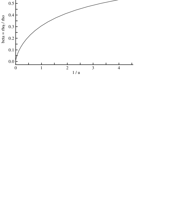
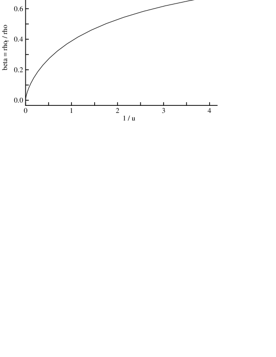
β(ρ0b)=0.552and 0.685𝛽superscriptsubscript𝜌0𝑏0.552and0.685\beta(\rho_{0}^{b})=0.552\ \ {\rm and}\ \ 0.685 (6)

for Models 1 and 2, respectively. Their numerical values in Models 1 and 2 are shown as functions of ρbsuperscript𝜌𝑏\rho^{b} in Figs.1 and 2, respectively.

The functional relation β(x)𝛽𝑥\beta(x) is expressed approximately using two analytic functions in Models 1 and 2 in terms of ux/[3(H0b)2]𝑢𝑥delimited-[]3superscriptsubscriptsuperscript𝐻𝑏02u\equiv x/[3(H^{b}_{0})^{2}] as follows.

Model 1:

β(x)=0.292(1/u)0.400[1+0.065/u0.0137/u2]𝛽𝑥0.292superscript1𝑢0.400delimited-[]10.065𝑢0.0137superscript𝑢2\beta(x)=0.292(1/u)^{0.400}[1+0.065/u-0.0137/u^{2}] (7)

for  (0.22)11/u0.982(1ab0.6)formulae-sequencesuperscript0.2211𝑢0.9821superscript𝑎𝑏0.6(0.22)^{-1}\geq 1/u\geq 0.982\quad(1\geq a^{b}\geq 0.6), and

β(x)=0.383(1/u)0.665[10.261/u+0.0627/u2]𝛽𝑥0.383superscript1𝑢0.665delimited-[]10.261𝑢0.0627superscript𝑢2\beta(x)=0.383(1/u)^{0.665}[1-0.261/u+0.0627/u^{2}] (8)

for  0.9821/u0(0.6ab0)formulae-sequence0.9821𝑢00.6superscript𝑎𝑏00.982\geq 1/u\geq 0\quad(0.6\geq a^{b}\geq 0), where absuperscript𝑎𝑏a^{b} is the scale-factor with the present value a0b=1subscriptsuperscript𝑎𝑏01a^{b}_{0}=1.

Model 2:

β(x)=0.362(1/u)0.400[1+0.0884/u0.0166/u2]𝛽𝑥0.362superscript1𝑢0.400delimited-[]10.0884𝑢0.0166superscript𝑢2\beta(x)=0.362(1/u)^{0.400}[1+0.0884/u-0.0166/u^{2}] (9)

for  (0.24)11/u0.9(1ab0.6)formulae-sequencesuperscript0.2411𝑢0.91superscript𝑎𝑏0.6(0.24)^{-1}\geq 1/u\geq 0.9\quad(1\geq a^{b}\geq 0.6), and

β(x)=0.459(1/u)0.665[1+0.074/u0.251/u2]𝛽𝑥0.459superscript1𝑢0.665delimited-[]10.074𝑢0.251superscript𝑢2\beta(x)=0.459(1/u)^{0.665}[1+0.074/u-0.251/u^{2}] (10)

for  0.9001/u0(0.6ab0)formulae-sequence0.9001𝑢00.6superscript𝑎𝑏00.900\geq 1/u\geq 0\quad(0.6\geq a^{b}\geq 0).


Figure 1: β𝛽\beta is expressed as a function of 1/u1𝑢1/u in Model 1. The ordinate is β(ρf/ρb)annotated𝛽absentsubscript𝜌𝑓superscript𝜌𝑏\beta\ (\equiv\rho_{f}/\rho^{b}) and uρb/[3(H0b)2]𝑢superscript𝜌𝑏delimited-[]3superscriptsubscriptsuperscript𝐻𝑏02u\equiv\rho^{b}/[3(H^{b}_{0})^{2}].

Refer to caption

Figure 2: β𝛽\beta is expressed as a function of 1/u1𝑢1/u in Model 2. The ordinate is β(ρf/ρb)annotated𝛽absentsubscript𝜌𝑓superscript𝜌𝑏\beta\ (\equiv\rho_{f}/\rho^{b}) and uρb/[3(H0b)2]𝑢superscript𝜌𝑏delimited-[]3superscriptsubscriptsuperscript𝐻𝑏02u\equiv\rho^{b}/[3(H^{b}_{0})^{2}].

Refer to caption


3 Cosmological models with the fluctuation energy and the model parameters

To derive a spatially flat model with the fluctuation energy, we consider the line element

ds2=gμνdxμdyν=a2(η)[dη2+δijdxidxj],𝑑superscript𝑠2subscript𝑔𝜇𝜈𝑑superscript𝑥𝜇𝑑superscript𝑦𝜈superscript𝑎2𝜂delimited-[]𝑑superscript𝜂2subscript𝛿𝑖𝑗𝑑superscript𝑥𝑖𝑑superscript𝑥𝑗ds^{2}=g_{\mu\nu}dx^{\mu}dy^{\nu}=a^{2}(\eta)[-d\eta^{2}+\delta_{ij}dx^{i}dx^{j}], (11)

where the Greek and Roman letters denote 0,1,2,301230,1,2,3 and 1,2,31231,2,3, respectively. The conformal time η(=x0)annotated𝜂absentsuperscript𝑥0\eta(=x^{0}) is related to the cosmic time t𝑡t by dt=a(η)dη𝑑𝑡𝑎𝜂𝑑𝜂dt=a(\eta)d\eta.

In this paper, the fluctuation energy is regarded as a kind of dark matter, and is assumed to move together with ordinary dust. Then the velocity vector and energy-momentum tensor of pressureless matter are expressed in comoving coordinates as

u0=1/a,ui=0formulae-sequencesuperscript𝑢01𝑎superscript𝑢𝑖0u^{0}=1/a,\quad u^{i}=0 (12)

and

T00=ρT,Ti0=0,Tji=0formulae-sequencesubscriptsuperscript𝑇00subscript𝜌𝑇formulae-sequencesubscriptsuperscript𝑇0𝑖0subscriptsuperscript𝑇𝑖𝑗0T^{0}_{0}=-\rho_{T},\quad T^{0}_{i}=0,\quad T^{i}_{j}=0 (13)

with ρTρ+ρfsubscript𝜌𝑇𝜌subscript𝜌𝑓\rho_{T}\equiv\rho+\rho_{f}, where ρT,ρ,subscript𝜌𝑇𝜌\rho_{T},\rho, and ρfsubscript𝜌𝑓\rho_{f} are the total density of pressureless matter, the ordinary dust density, and the fluctuation energy density, respectively, and we assume

ρf=ρβ(ρ)subscript𝜌𝑓𝜌𝛽𝜌\rho_{f}=\rho\ \beta(\rho) (14)

as the approximate equation of state for the fluctuation energy, where the function β(ρ)𝛽𝜌\beta(\rho) is specified by Eq.(5) with Figs. 1 and 2, and Eqs.(7) similar-to\sim (10).

From the Einstein equations, we obtain

ρTa2=3(a/a)2Λa2,subscript𝜌𝑇superscript𝑎23superscriptsuperscript𝑎𝑎2Λsuperscript𝑎2\rho_{T}a^{2}=3(a^{\prime}/a)^{2}-\Lambda a^{2}, (15)

and the energy-momentum conservation (T;νμν=0T^{\mu\nu}_{;\nu}=0) gives the relation

ρTa3=ρT(t0),subscript𝜌𝑇superscript𝑎3subscript𝜌𝑇subscript𝑡0\rho_{T}a^{3}=\rho_{T}(t_{0}), (16)

where a=1𝑎1a=1 at the present epoch (t=t0𝑡subscript𝑡0t=t_{0}) and a prime denotes /η𝜂\partial/\partial\eta. In the previous paper(tompre, ), the renormalization of the Hubble constant was done using the spatial average of the second-order metric perturbation. In this paper, the Hubble parameter is derived only through considering the fluctuation energy ρfsubscript𝜌𝑓\rho_{f} as the part of the total energy. Then the Hubble parameter H(a˙/a=a/a2)H(\equiv\dot{a}/a=a^{\prime}/a^{2}) satisfies

H2=13(ρT+Λ)=13(ρ+ρf+Λ)superscript𝐻213subscript𝜌𝑇Λ13𝜌subscript𝜌𝑓ΛH^{2}=\frac{1}{3}(\rho_{T}+\Lambda)=\frac{1}{3}(\rho+\rho_{f}+\Lambda) (17)

and we have the relations for the model parameters

ΩMΩMd+ΩMf,subscriptΩ𝑀subscriptΩ𝑀𝑑subscriptΩ𝑀𝑓\Omega_{M}\equiv\Omega_{Md}+\Omega_{Mf}, (18)

and

ΩMd13ρ(t0)(H0)2,ΩMf13ρf(t0)(H0)2,formulae-sequencesubscriptΩ𝑀𝑑13𝜌subscript𝑡0superscriptsubscript𝐻02subscriptΩ𝑀𝑓13subscript𝜌𝑓subscript𝑡0superscriptsubscript𝐻02\Omega_{Md}\equiv\frac{1}{3}\frac{\rho(t_{0})}{(H_{0})^{2}},\quad\Omega_{Mf}\equiv\frac{1}{3}\frac{\rho_{f}(t_{0})}{(H_{0})^{2}}, (19)

where H0subscript𝐻0H_{0} is H𝐻H at the present epoch (t0subscript𝑡0t_{0}). This model reduces to the basic background models in Sect. 2 in the limit a0𝑎0a\rightarrow 0, because ρf/ρ0subscript𝜌𝑓𝜌0\rho_{f}/\rho\rightarrow 0.

From Eqs.(15) and (18), the equation for a𝑎a is

a=H0[a(ΩM+ΩΛa3)]1/2,superscript𝑎subscript𝐻0superscriptdelimited-[]𝑎subscriptΩ𝑀subscriptΩΛsuperscript𝑎312a^{\prime}=H_{0}[a(\Omega_{M}+\Omega_{\Lambda}a^{3})]^{1/2}, (20)

and a(t)𝑎𝑡a(t) is determined by specifying ΩM,ΩΛsubscriptΩ𝑀subscriptΩΛ\Omega_{M},\Omega_{\Lambda}, and H0subscript𝐻0H_{0}, and solving this equation.

Now let us derive the model parameters (ΩM,ΩΛ,H0)subscriptΩ𝑀subscriptΩΛsubscript𝐻0(\Omega_{M},\Omega_{\Lambda},H_{0}) in the present model as the function of (ΩMb,ΩΛb,H0b)superscriptsubscriptΩ𝑀𝑏superscriptsubscriptΩΛ𝑏superscriptsubscript𝐻0𝑏(\Omega_{M}^{b},\Omega_{\Lambda}^{b},H_{0}^{b}) in the basic models. Here the Hubble parameters are represented by H𝐻H and Hbsuperscript𝐻𝑏H^{b} at epochs with scale factors a𝑎a and absuperscript𝑎𝑏a^{b}, respectively, and their ratio α𝛼\alpha is expressed as

α2(H/Hb)2=(1+β)ρ+Λρb+Λsuperscript𝛼2superscript𝐻superscript𝐻𝑏21𝛽𝜌Λsuperscript𝜌𝑏Λ\alpha^{2}\equiv(H/H^{b})^{2}=\frac{(1+\beta)\rho+\Lambda}{\rho^{b}+\Lambda} (21)

using Eqs. (4) and (17). This equation is rewritten as

ρ/ρb=[(α21)Λ/ρb+α2]/(1+β).𝜌superscript𝜌𝑏delimited-[]superscript𝛼21Λsuperscript𝜌𝑏superscript𝛼21𝛽\rho/\rho^{b}=[(\alpha^{2}-1)\Lambda/\rho^{b}+\alpha^{2}]/(1+\beta). (22)

At the present epoch with a=ab=1𝑎superscript𝑎𝑏1a=a^{b}=1, we have

(α0)2=ΩΛb+(1+β0)ΩMb(ρ/ρb)0superscriptsubscript𝛼02superscriptsubscriptΩΛ𝑏1subscript𝛽0superscriptsubscriptΩ𝑀𝑏subscript𝜌superscript𝜌𝑏0(\alpha_{0})^{2}=\Omega_{\Lambda}^{b}+(1+\beta_{0})\Omega_{M}^{b}(\rho/\rho^{b})_{0}\ (23)

or

(ρ/ρb)0=X/(1+β0),subscript𝜌superscript𝜌𝑏0𝑋1subscript𝛽0(\rho/\rho^{b})_{0}=X/(1+\beta_{0}), (24)

where (α0,β0)subscript𝛼0subscript𝛽0(\alpha_{0},\beta_{0}) is the present counterpart of (α,β)𝛼𝛽(\alpha,\beta) and

X[(α0)21]ΩΛb/ΩMb+(α0)2.𝑋delimited-[]superscriptsubscript𝛼021superscriptsubscriptΩΛ𝑏superscriptsubscriptΩ𝑀𝑏superscriptsubscript𝛼02X\equiv[(\alpha_{0})^{2}-1]\Omega_{\Lambda}^{b}/\Omega_{M}^{b}+(\alpha_{0})^{2}. (25)

Here we express ΩMd,ΩMf,subscriptΩ𝑀𝑑subscriptΩ𝑀𝑓\Omega_{Md},\Omega_{Mf}, and ΩΛsubscriptΩΛ\Omega_{\Lambda} in terms of ΩMbsuperscriptsubscriptΩ𝑀𝑏\Omega_{M}^{b} and ΩΛbsuperscriptsubscriptΩΛ𝑏\Omega_{\Lambda}^{b}. Using Eq.(23), we obtain

(ΩMd,ΩMf,ΩΛ)=13(H0)2(ρ0,ρf0,Λ)=(ρ0,ρf0,Λ)3(α0)2(H0b)2.subscriptΩ𝑀𝑑subscriptΩ𝑀𝑓subscriptΩΛ13superscriptsubscript𝐻02subscript𝜌0subscript𝜌𝑓0Λsubscript𝜌0subscript𝜌𝑓0Λ3superscriptsubscript𝛼02superscriptsuperscriptsubscript𝐻0𝑏2(\Omega_{Md},\Omega_{Mf},\Omega_{\Lambda})=\frac{1}{3(H_{0})^{2}}(\rho_{0},\rho_{f0},\Lambda)=\frac{(\rho_{0},\rho_{f0},\Lambda)}{3(\alpha_{0})^{2}(H_{0}^{b})^{2}}. (26)

Using Eq.(24), moreover, we obtain

(ΩMd,ΩMf,ΩΛ)=ΩMb(α0)2(X1+β0,β0X1+β0,ΩΛbΩMb).subscriptΩ𝑀𝑑subscriptΩ𝑀𝑓subscriptΩΛsuperscriptsubscriptΩ𝑀𝑏superscriptsubscript𝛼02𝑋1subscript𝛽0subscript𝛽0𝑋1subscript𝛽0superscriptsubscriptΩΛ𝑏superscriptsubscriptΩ𝑀𝑏(\Omega_{Md},\Omega_{Mf},\Omega_{\Lambda})=\frac{\Omega_{M}^{b}}{(\alpha_{0})^{2}}(\frac{X}{1+\beta_{0}},\frac{\beta_{0}X}{1+\beta_{0}},\frac{\Omega_{\Lambda}^{b}}{\Omega_{M}^{b}}). (27)

For the density parameter of the pressureless matter ΩM(ΩMd+ΩMf)annotatedsubscriptΩ𝑀absentsubscriptΩ𝑀𝑑subscriptΩ𝑀𝑓\Omega_{M}\ (\equiv\Omega_{Md}+\Omega_{Mf}), we have

(ΩM,ΩΛ)=ΩMb(α0)2(X,ΩΛb/ΩMb),subscriptΩ𝑀subscriptΩΛsuperscriptsubscriptΩ𝑀𝑏superscriptsubscript𝛼02𝑋superscriptsubscriptΩΛ𝑏superscriptsubscriptΩ𝑀𝑏(\Omega_{M},\Omega_{\Lambda})=\frac{\Omega_{M}^{b}}{(\alpha_{0})^{2}}(X,\Omega_{\Lambda}^{b}/\Omega_{M}^{b}), (28)

and for ordinary dust, we have

(ΩMd,ΩMf+ΩΛ)=ΩMb(α0)2(X1+β0,β01+β0X+ΩΛb/ΩMb).subscriptΩ𝑀𝑑subscriptΩ𝑀𝑓subscriptΩΛsuperscriptsubscriptΩ𝑀𝑏superscriptsubscript𝛼02𝑋1subscript𝛽0subscript𝛽01subscript𝛽0𝑋superscriptsubscriptΩΛ𝑏superscriptsubscriptΩ𝑀𝑏(\Omega_{Md},\Omega_{Mf}+\Omega_{\Lambda})=\frac{\Omega_{M}^{b}}{(\alpha_{0})^{2}}(\frac{X}{1+\beta_{0}},\frac{\beta_{0}}{1+\beta_{0}}X+\Omega_{\Lambda}^{b}/\Omega_{M}^{b}). (29)

Here we consider the correspondence between the ordinary dust density in the model with ρf0subscript𝜌𝑓0\rho_{f}\neq 0 and that in the basic model (ρf=0subscript𝜌𝑓0\rho_{f}=0), so that we may clarify the additional effect of the fluctuation energy. First we take the correspondence in which the present densities of ordinary dust are equal, i.e.,

(ρ/ρb)0=1.subscript𝜌superscript𝜌𝑏01(\rho/\rho^{b})_{0}=1. (30)

Then we obtain X=1+β0𝑋1subscript𝛽0X=1+\beta_{0} and

(α0)2=ΩMb(1+β0)+ΩΛbsuperscriptsubscript𝛼02superscriptsubscriptΩ𝑀𝑏1subscript𝛽0superscriptsubscriptΩΛ𝑏(\alpha_{0})^{2}=\Omega_{M}^{b}(1+\beta_{0})+\Omega_{\Lambda}^{b} (31)

from Eq.(23). For inserting β0β(ρ0)subscript𝛽0𝛽subscript𝜌0\beta_{0}\equiv\beta(\rho_{0}) and the model parameters of the two basic models, therefore, we obtain

α0=1.059,(ΩM,ΩΛ)=(0.305,0.695)andH0=71.3kms1Mpc1formulae-sequencesubscript𝛼01.059subscriptΩ𝑀subscriptΩΛ0.3050.695andsubscript𝐻071.3kmsuperscripts1superscriptMpc1\begin{split}\alpha_{0}&=1.059,\cr(\Omega_{M},\Omega_{\Lambda})&=(0.305,0.695)\ {\rm and}\ H_{0}=71.3\ {\rm km\ s^{-1}Mpc^{-1}}\end{split} (32)

for Model 1, and

α0=1.079,(ΩM,ΩΛ)=(0.347,0.653)andH0=72.6kms1Mpc1formulae-sequencesubscript𝛼01.079subscriptΩ𝑀subscriptΩΛ0.3470.653andsubscript𝐻072.6kmsuperscripts1superscriptMpc1\begin{split}\alpha_{0}&=1.079,\cr(\Omega_{M},\Omega_{\Lambda})&=(0.347,0.653)\ {\rm and}\ H_{0}=72.6\ {\rm km\ s^{-1}Mpc^{-1}}\end{split} (33)

for Model 2.

For the present ordinary dust density ratio (ρ/ρb)0subscript𝜌superscript𝜌𝑏0(\rho/\rho^{b})_{0} which is not equal to 111, we have X=(ρ/ρb)0(1+β0)𝑋subscript𝜌superscript𝜌𝑏01subscript𝛽0X=(\rho/\rho^{b})_{0}(1+\beta_{0}) from Eq.(24), and, using Eq.(23) for α0subscript𝛼0\alpha_{0}, we obtain the following parameters for the model parameters of the two basic models and several values of (ρ/ρb)0subscript𝜌superscript𝜌𝑏0(\rho/\rho^{b})_{0} :

(ρ/ρb)0=1.181,α0=1.088,(ΩM,ΩΛ)=(0.341,0.659),andH0=73.2kms1Mpc1\begin{split}(\rho/\rho^{b})_{0}&=1.181,\quad\alpha_{0}=1.088,\cr(\Omega_{M},\Omega_{\Lambda})&=(0.341,0.659),\ {\rm and}\ H_{0}=73.2\ {\rm km\ s^{-1}Mpc^{-1}}\end{split} (34)

for Model 1, and

(ρ/ρb)0=1.110,α0=1.099,(ΩM,ΩΛ)=(0.371,0.629),andH0=74.0kms1Mpc1,\begin{split}(\rho/\rho^{b})_{0}&=1.110,\quad\alpha_{0}=1.099,\cr(\Omega_{M},\Omega_{\Lambda})&=(0.371,0.629),\ {\rm and}\ H_{0}=74.0\ {\rm km\ s^{-1}Mpc^{-1}},\end{split} (35)

and

(ρ/ρb)0=1.276,α0=1.130,(ΩM,ΩΛ)=(0.404,0.596),andH0=76.0kms1Mpc1\begin{split}(\rho/\rho^{b})_{0}&=1.276,\quad\alpha_{0}=1.130,\cr(\Omega_{M},\Omega_{\Lambda})&=(0.404,0.596),\ {\rm and}\ H_{0}=76.0\ {\rm km\ s^{-1}Mpc^{-1}}\end{split} (36)

for Model 2.

Thus, we obtained model parameters in the models with fluctuation energy by specifying the basic model parameters and (ρ/ρb)0subscript𝜌superscript𝜌𝑏0(\rho/\rho^{b})_{0} for their correspondence. The above model parameters with the fluctuation energy are comparable with the observed ones.(planck1, ; planck2, ; h1, ; h2, ; h3, ; h4, ; decay, ) Those with (ρ/ρb)0=1subscript𝜌superscript𝜌𝑏01(\rho/\rho^{b})_{0}=1 in Model 2 and (ρ/ρb)0=1.181subscript𝜌superscript𝜌𝑏01.181(\rho/\rho^{b})_{0}=1.181 in Model 1 are near to the observed ones with H0=7374kms1Mpc1subscript𝐻073similar-to74kmsuperscripts1superscriptMpc1H_{0}=73\sim 74\ {\rm km\ s^{-1}Mpc^{-1}}.

Next let us study the behaviors of models in the past in comparison with the basic models. Here α(H/Hb)annotated𝛼absent𝐻superscript𝐻𝑏\alpha\ (\equiv H/H^{b}) is obtained from Eq. (21) as

α2=(ρT)0/a3+Λ(ρb/ρT)(ρT)0/a3+Λ=(1+β0)(ρ/ρb)0ΩMb+ΩΛba31+β01+β(ρ/ρb)0ρ/ρbΩMb+ΩΛba3,superscript𝛼2subscriptsubscript𝜌𝑇0superscript𝑎3Λsuperscript𝜌𝑏subscript𝜌𝑇subscriptsubscript𝜌𝑇0superscript𝑎3Λ1subscript𝛽0subscript𝜌superscript𝜌𝑏0superscriptsubscriptΩ𝑀𝑏subscriptsuperscriptΩ𝑏Λsuperscript𝑎31subscript𝛽01𝛽subscript𝜌superscript𝜌𝑏0𝜌superscript𝜌𝑏superscriptsubscriptΩ𝑀𝑏subscriptsuperscriptΩ𝑏Λsuperscript𝑎3\alpha^{2}=\frac{(\rho_{T})_{0}/a^{3}+\Lambda}{(\rho^{b}/\rho_{T})(\rho_{T})_{0}/a^{3}+\Lambda}=\frac{(1+\beta_{0})(\rho/\rho^{b})_{0}\Omega_{M}^{b}+\Omega^{b}_{\Lambda}a^{3}}{\frac{1+\beta_{0}}{1+\beta}\frac{(\rho/\rho^{b})_{0}}{\rho/\rho^{b}}\Omega_{M}^{b}+\Omega^{b}_{\Lambda}a^{3}}, (37)

where β(ρ)𝛽𝜌\beta(\rho) is given by Eqs. (7) - (10), and

a3=ρT(t0)/ρT=(ρ0/ρ)1+β01+β(ρ).superscript𝑎3subscript𝜌𝑇subscript𝑡0subscript𝜌𝑇subscript𝜌0𝜌1subscript𝛽01𝛽𝜌a^{3}=\rho_{T}(t_{0})/\rho_{T}=(\rho_{0}/\rho)\frac{1+\beta_{0}}{1+\beta(\rho)}. (38)

To evaluate α𝛼\alpha in the past for (ρ/ρb)0=1subscript𝜌superscript𝜌𝑏01(\rho/\rho^{b})_{0}=1, we take the correspondence between a𝑎a and absuperscript𝑎𝑏a^{b}, in such a way that ρ/ρb=1𝜌superscript𝜌𝑏1\rho/\rho^{b}=1 also in the past. Then we have

α2=(1+β0)ΩMb+ΩΛba31+β01+βΩMb+ΩΛba3,superscript𝛼21subscript𝛽0superscriptsubscriptΩ𝑀𝑏subscriptsuperscriptΩ𝑏Λsuperscript𝑎31subscript𝛽01𝛽superscriptsubscriptΩ𝑀𝑏subscriptsuperscriptΩ𝑏Λsuperscript𝑎3\alpha^{2}=\frac{(1+\beta_{0})\Omega_{M}^{b}+\Omega^{b}_{\Lambda}a^{3}}{\frac{1+\beta_{0}}{1+\beta}\Omega_{M}^{b}+\Omega^{b}_{\Lambda}a^{3}}, (39)

so that β0𝛽0\beta\rightarrow 0 and α1𝛼1\alpha\rightarrow 1 for a0𝑎0a\rightarrow 0.

To evaluate α𝛼\alpha in the past for (ρ/ρb)01subscript𝜌superscript𝜌𝑏01(\rho/\rho^{b})_{0}\neq 1, we take the correspondence in such a way that

ρ/ρb=[(ρ/ρb)01](ρ0b/ρb)+1.𝜌superscript𝜌𝑏delimited-[]subscript𝜌superscript𝜌𝑏01subscriptsuperscript𝜌𝑏0superscript𝜌𝑏1\rho/\rho^{b}=[(\rho/\rho^{b})_{0}-1](\rho^{b}_{0}/\rho^{b})+1. (40)

Then we find that ρ/ρb1𝜌superscript𝜌𝑏1\rho/\rho^{b}\rightarrow 1 and β0𝛽0\beta\rightarrow 0 for a0𝑎0a\rightarrow 0, and from Eq.(37) that α1𝛼1\alpha\rightarrow 1 for a0𝑎0a\rightarrow 0.

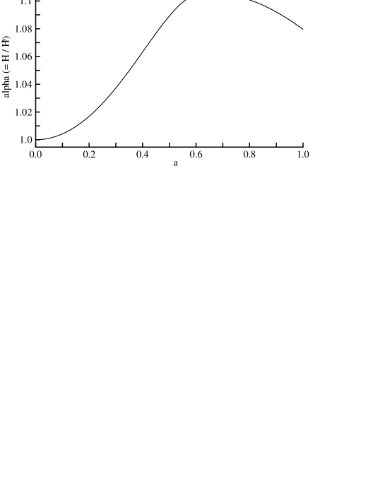
The a𝑎a dependences of 1/u,β1𝑢𝛽1/u,\beta and α𝛼\alpha in the case of (ρ/ρb)0=1subscript𝜌superscript𝜌𝑏01(\rho/\rho^{b})_{0}=1 for Model 2 (with the model parameter (33)) are shown in Figs. 3, 4 and 5, respectively, where uρ/[3(H0b)2]𝑢𝜌delimited-[]3superscriptsuperscriptsubscript𝐻0𝑏2u\equiv\rho/[3(H_{0}^{b})^{2}]. At the early stage with a<0.6𝑎0.6a<0.6, the role of ρfsubscript𝜌𝑓\rho_{f} is effective and α𝛼\alpha increases with a𝑎a, but at the later stage with 1.0>a>0.61.0𝑎0.61.0>a>0.6, ΛΛ\Lambda is dominant and α𝛼\alpha decreases slowly after a peak.

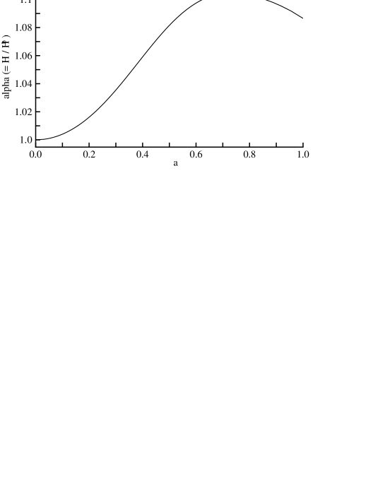
The a𝑎a dependences of 1/u,β1𝑢𝛽1/u,\beta and α𝛼\alpha in the case of (ρ/ρb)01subscript𝜌superscript𝜌𝑏01(\rho/\rho^{b})_{0}\neq 1 are also found to be similar to those in the case of (ρ/ρb)0=1subscript𝜌superscript𝜌𝑏01(\rho/\rho^{b})_{0}=1, owing to the above correspondence. Here the a𝑎a dependence of α𝛼\alpha in the case of (ρ/ρb)01subscript𝜌superscript𝜌𝑏01(\rho/\rho^{b})_{0}\neq 1 for Model 1 (with the model parameter (34)) is shown in Fig. 6.

Moreover, let us define the time-dependent model parameters ΩM(t)subscriptΩ𝑀𝑡\Omega_{M}(t) and ΩMb(t)superscriptsubscriptΩ𝑀𝑏𝑡\Omega_{M}^{b}(t) (representing those in the past) by

ΩM(t)ρT3H2andΩMb(t)ρb3(Hb)2.formulae-sequencesubscriptΩ𝑀𝑡subscript𝜌𝑇3superscript𝐻2andsuperscriptsubscriptΩ𝑀𝑏𝑡superscript𝜌𝑏3superscriptsuperscript𝐻𝑏2\Omega_{M}(t)\equiv\frac{\rho_{T}}{3H^{2}}\quad{\rm and}\quad\Omega_{M}^{b}(t)\equiv\frac{\rho^{b}}{3(H^{b})^{2}}. (41)

Then ΩM=ΩM(t0)subscriptΩ𝑀subscriptΩ𝑀subscript𝑡0\Omega_{M}=\Omega_{M}(t_{0}) and ΩMb=ΩMb(t0)superscriptsubscriptΩ𝑀𝑏superscriptsubscriptΩ𝑀𝑏subscript𝑡0\Omega_{M}^{b}=\Omega_{M}^{b}(t_{0}), and we have the ratio

ΩM(t)/ΩMb(t)=(ρ/ρb)(1+β)/α2.subscriptΩ𝑀𝑡superscriptsubscriptΩ𝑀𝑏𝑡𝜌superscript𝜌𝑏1𝛽superscript𝛼2\Omega_{M}(t)/\Omega_{M}^{b}(t)=(\rho/\rho^{b})(1+\beta)/\alpha^{2}. (42)

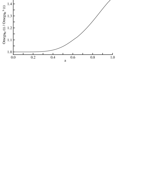
This ratio tends to 111 for a0𝑎0a\rightarrow 0. The a𝑎a dependence of ΩM(t)/ΩMb(t)subscriptΩ𝑀𝑡superscriptsubscriptΩ𝑀𝑏𝑡\Omega_{M}(t)/\Omega_{M}^{b}(t) is shown in Fig. 7 for the model parameter (33).

It is concluded, therefore, that at the later stage the models with the fluctuation energy can have a Hubble constant (H0=7374kms1Mpc1subscript𝐻073similar-to74kmsuperscripts1superscriptMpc1H_{0}=73\sim 74\ {\rm km\ s^{-1}Mpc^{-1}}) larger than that (H0b=67.3kms1Mpc1superscriptsubscript𝐻0𝑏67.3kmsuperscripts1superscriptMpc1H_{0}^{b}=67.3\ {\rm km\ s^{-1}Mpc^{-1}}) in the basic models, while, at the early stage with large densities, both models have the same Hubble constants (in such a way that H/Hb1𝐻superscript𝐻𝑏1H/H^{b}\rightarrow 1 for a0𝑎0a\rightarrow 0). This shows that the Hubble-constant problem(planck1, ; planck2, ; h1, ; h2, ; h3, ; h4, ; decay, ) can be solved by taking the fluctuation energy into account.
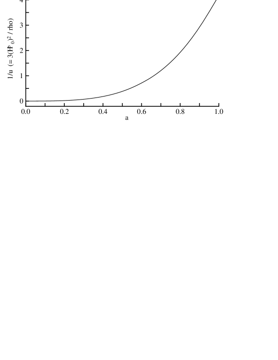
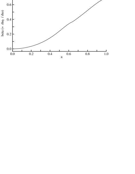
Figure 3: The (1/ua)1𝑢𝑎(1/u-a) relation in the case of (ρ/ρb)0=1subscript𝜌superscript𝜌𝑏01(\rho/\rho^{b})_{0}=1. The ordinate is 1/u1𝑢1/u, where uρ/[3(H0b)2]𝑢𝜌delimited-[]3superscriptsuperscriptsubscript𝐻0𝑏2u\equiv\rho/[3(H_{0}^{b})^{2}]. a𝑎a is the scale-factor and a=1𝑎1a=1 at the present epoch.

Refer to caption

Figure 4: The (βa)𝛽𝑎(\beta-a) relation in the case of (ρ/ρb)0=1subscript𝜌superscript𝜌𝑏01(\rho/\rho^{b})_{0}=1. The ordinate is β(ρf/ρ)annotated𝛽absentsubscript𝜌𝑓𝜌\beta\ (\equiv\rho_{f}/\rho).

Refer to caption

Figure 5: The (αa)𝛼𝑎(\alpha-a) relation in the case of (ρ/ρb)0=1subscript𝜌superscript𝜌𝑏01(\rho/\rho^{b})_{0}=1. The ordinate is α(H/Hb)annotated𝛼absent𝐻superscript𝐻𝑏\alpha\ (\equiv H/H^{b}). a𝑎a is the scale-factor and a=1𝑎1a=1 at the present epoch.

Refer to caption

Figure 6: The (αa)𝛼𝑎(\alpha-a) relation in the case of (ρ/ρb)0=1.181subscript𝜌superscript𝜌𝑏01.181(\rho/\rho^{b})_{0}=1.181. The ordinate is α(H/Hb)annotated𝛼absent𝐻superscript𝐻𝑏\alpha\ (\equiv H/H^{b}).

Refer to caption

Figure 7: The (ΩM(t)/ΩMb(t)a)subscriptΩ𝑀𝑡superscriptsubscriptΩ𝑀𝑏𝑡𝑎(\Omega_{M}(t)/\Omega_{M}^{b}(t)-a) relation in the case of (ρ/ρb)0=1subscript𝜌superscript𝜌𝑏01(\rho/\rho^{b})_{0}=1. The ordinate is ΩM(t)/ΩMb(t)subscriptΩ𝑀𝑡superscriptsubscriptΩ𝑀𝑏𝑡\Omega_{M}(t)/\Omega_{M}^{b}(t).

Refer to caption

4 Perturbations in cosmological models with the fluctuation energy

The behaviors of linear perturbations in the cosmological models with pressureless matter are well-known and expressed using the gauge-invariant treatment(bar, ; kodama, ).

Here we assume that the accurate background model has been obtained and consider the perturbations to it. The gauge-invariant density perturbation ϵTsubscriptitalic-ϵ𝑇\epsilon_{T} for the total density ρT(ρ+ρf)annotatedsubscript𝜌𝑇absent𝜌subscript𝜌𝑓\rho_{T}\ (\equiv\rho+\rho_{f}) satisfies the equation

ϵT′′+aaϵT12(ρTa2)ϵT=0.superscriptsubscriptitalic-ϵ𝑇′′superscript𝑎𝑎superscriptsubscriptitalic-ϵ𝑇12subscript𝜌𝑇superscript𝑎2subscriptitalic-ϵ𝑇0\epsilon_{T}^{\prime\prime}+\frac{a^{\prime}}{a}\epsilon_{T}^{\prime}-\frac{1}{2}(\rho_{T}a^{2})\epsilon_{T}=0. (43)

The evolutionary relation for the fluctuation energy is assumed to hold in the weak inhomogeneities. Then the gauge-invariant density perturbation ϵitalic-ϵ\epsilon for ordinary dust satisfies

ϵT=(1+dρf/dρ)ϵ=(1+β+ρdβ/dρ)ϵ,subscriptitalic-ϵ𝑇1𝑑subscript𝜌𝑓𝑑𝜌italic-ϵ1𝛽𝜌𝑑𝛽𝑑𝜌italic-ϵ\epsilon_{T}=(1+d\rho_{f}/d\rho)\epsilon=(1+\beta+\rho d\beta/d\rho)\epsilon, (44)

and the perturbation ϵfsubscriptitalic-ϵ𝑓\epsilon_{f} of the fluctuation energy is expressed as

ϵfϵTϵ=ϵT(β+ρdβ/dρ)/(1+β+ρdβ/dρ),subscriptitalic-ϵ𝑓subscriptitalic-ϵ𝑇italic-ϵsubscriptitalic-ϵ𝑇𝛽𝜌𝑑𝛽𝑑𝜌1𝛽𝜌𝑑𝛽𝑑𝜌\epsilon_{f}\equiv\epsilon_{T}-\epsilon=\epsilon_{T}(\beta+\rho d\beta/d\rho)/(1+\beta+\rho d\beta/d\rho), (45)

and

ϵ=ϵT/(1+β+ρdβ/dρ).italic-ϵsubscriptitalic-ϵ𝑇1𝛽𝜌𝑑𝛽𝑑𝜌\epsilon=\epsilon_{T}/(1+\beta+\rho d\beta/d\rho). (46)

At the early stage of β1much-less-than𝛽1\beta\ll 1, ϵϵTsimilar-to-or-equalsitalic-ϵsubscriptitalic-ϵ𝑇\epsilon\simeq\epsilon_{T} and ϵfϵmuch-less-thansubscriptitalic-ϵ𝑓italic-ϵ\epsilon_{f}\ll\epsilon, but at the later stage of β1similar-to𝛽1\beta\sim 1, ϵitalic-ϵ\epsilon and ϵfsubscriptitalic-ϵ𝑓\epsilon_{f} are comparable.

5 Concluding remarks

The existence of random fluctuations is beyond doubt and their amplitudes are also well-known(wein, ; ll, ; dodel, ; tsuji, ; bbks, ). We must take their energy (the fluctuation energy) into account, to clarify the dynamical evolution of the universe. This paper is the first step to considering it as a kind of dark matter.

At the stage of a1much-less-than𝑎1a\ll 1, the fluctuation energy ρfsubscript𝜌𝑓\rho_{f} is negligibly small compared with the density ρ𝜌\rho of ordinary dust, but at the present epoch it occupies about 3641%similar-to36percent4136\sim 41\% of the total density of the pressureless matter, depending on the basic models. The fluctuation energy was considered in this paper as part of the dark matter, which cannot be touched but contributes to the formation and evolution of astronomical objects at the later stage. The essential difference between the model with the fluctuation energy and the basic models is the quantitative large change in the dark matter.

In this paper we tentatively adopted Model 1 and Model 2 as the basic model, to derive the fluctuation energy using the second-order perturbation theory. The derived model parameters depend sensitively on their basic model parameters, the present ordinary dust density ratio (ρ/ρb)0subscript𝜌superscript𝜌𝑏0(\rho/\rho^{b})_{0}, and the upper limit xmaxsubscript𝑥𝑚𝑎𝑥x_{max} for the integrations A𝐴A and B𝐵B (in Appendix A). Therefore, they should be selected, so that the derived model parameters may be fitted as well as possible with the observational ones.

In the previous paper(tompre, ), we took the effect of fluctuation energy into account, by renormalizing the model parameters of a basic background model due to adding the second-order density and metric perturbations to the background quantities. That method is different from the present one in which the cosmological models are constructed by taking the fluctuation energy into account as part of pressureless matter. However, we could obtain similar model parameters that are consistent with their observational values.

The accuracy for the second-order perturbations ρf(δ2ρ)annotatedsubscript𝜌𝑓absentsubscript𝛿2𝜌\rho_{f}\ (\equiv\delta_{2}\rho) is good at the early stage of the universe, because βρf/ρ1𝛽subscript𝜌𝑓𝜌much-less-than1\beta\equiv\rho_{f}/\rho\ll 1, but it becomes worse with the expansion of the universe. At the present epoch, β𝛽\beta is still smaller than 111, but not so small, i.e. 0.5520.5520.552 and 0.6850.6850.685 for the two basic models as Eq. (6) shows. So, to derive a more accurate model at the stage of a1similar-to-or-equals𝑎1a\simeq 1, we should correct β(x)𝛽𝑥\beta(x) in Eq.(7) - Eq.(10), by constructing the higher-order general-relativistic perturbation theories.

The contributions of the super-sample modes (i.e. the large-scale modes longer than the survey scales) to the mean density fluctuations and the power spectrum in the finite-volume survey have recently been studied by several authors.(TH, ; LHT, ) They are not equal to the backreaction of long-wavelength random fluctuations, but they may be closely connected with it, and so with the present analyses. If so, the general-relativistic second-order perturbations, or the nonlinear perturbations in the post-Newtonian approximation may play important roles also in their treatments (in the similar way to our treatment in the previous paper(tompre, )). This is because the large-scale modes cross the Hubble-scale length during their evolution from the very early stage to the present epoch.(baldauf, )


Acknowledgement

The author thanks the referee for helpful comments.

Appendix A Second-order density perturbations corresponding to the first-order random fluctuations

In the Sect. 3 of the previous paper(tompre, ), we obtained the formula for the spatial average of the second-order density perturbations in the basic models. It is expressed as

𝛿2ρ/ρ~=4π3(Keq)4𝒫0[1Y(a)](ΩM/a+ΩΛa2)[112(Keq)2A+Z(a)B],delimited-⟨⟩subscript𝛿2𝜌~𝜌4𝜋3superscriptsubscript𝐾𝑒𝑞4subscript𝒫0delimited-[]1𝑌𝑎subscriptΩ𝑀𝑎subscriptΩΛsuperscript𝑎2delimited-[]112superscriptsubscript𝐾𝑒𝑞2𝐴𝑍𝑎𝐵\langle\mathop{\delta}_{2}\rho/\tilde{\rho}\rangle=\frac{4\pi}{3}\ (K_{eq})^{4}\ {\cal P}_{{\cal R}0}\ \frac{[1-Y(a)]}{(\Omega_{M}/a+\Omega_{\Lambda}a^{2})}\Big{[}\frac{11}{2}\ (K_{eq})^{-2}A+Z(a)B\Big{]}, (47)

where 𝒫0=2.2×10⁹,ρ~=ρ+Λ,H0b=100h,formulae-sequencesubscript𝒫02.2superscript109formulae-sequence~𝜌𝜌Λsuperscriptsubscript𝐻0𝑏100{\cal P}_{{\cal R}0}=2.2\times 10^{-9},\ \tilde{\rho}=\rho+\Lambda,\ H_{0}^{b}=100h, and Keqkeq/H0b=219(ΩMbh).subscript𝐾𝑒𝑞subscript𝑘𝑒𝑞superscriptsubscript𝐻0𝑏219superscriptsubscriptΩ𝑀𝑏K_{eq}\equiv k_{eq}/H_{0}^{b}=219(\Omega_{M}^{b}h).

For h=0.6730.673h=0.673, we have

Keq=32.4(ΩMb/0.22).subscript𝐾𝑒𝑞32.4superscriptsubscriptΩ𝑀𝑏0.22K_{eq}=32.4(\Omega_{M}^{b}/0.22). (48)

For the transfer function Ts(x)subscript𝑇𝑠𝑥T_{s}(x), A𝐴A and B𝐵B are expressed as

Axminxmax𝑑xxTs2(x),Bxminxmax𝑑xx3Ts2(x),formulae-sequence𝐴subscriptsuperscriptsubscript𝑥𝑚𝑎𝑥subscript𝑥𝑚𝑖𝑛differential-d𝑥𝑥superscriptsubscript𝑇𝑠2𝑥𝐵subscriptsuperscriptsubscript𝑥𝑚𝑎𝑥subscript𝑥𝑚𝑖𝑛differential-d𝑥superscript𝑥3superscriptsubscript𝑇𝑠2𝑥A\equiv\int^{x_{max}}_{x_{min}}dx\ x\ T_{s}^{2}(x),\quad B\equiv\int^{x_{max}}_{x_{min}}dx\ x^{3}\ T_{s}^{2}(x), (49)

where xk/keq𝑥𝑘subscript𝑘𝑒𝑞x\equiv k/k_{eq} for the wave-number k𝑘k, and the upper and lower limits of the integrations are specified by xmax=5.7subscript𝑥𝑚𝑎𝑥5.7x_{max}=5.7 and xmin=0.01subscript𝑥𝑚𝑖𝑛0.01x_{min}=0.01.

The definitions of Y(a),𝑌𝑎Y(a), and Z(a)𝑍𝑎Z(a) are found in the previous paper(tompre, ).

References

  • (1) S. Weinberg, Cosmology (Oxford University Press, New York, 2008).
  • (2) A. R. Liddle and D.H. Lyth, Cosmological Inflation and Large-Scale Structure (Cambridge University Press, New York, 2000).
  • (3) J.A. Peacock, Cosmological Physics (Cambridge University Press, Cambridge, 1999).
  • (4) L. Amendola and S. Tsujikawa, Dark Energy (Cambridge University Press, Cambridge, 2010).
  • (5) J. M. Bardeen, J. R. Bond, N. Kaiser, and A.S. Szalay, Astrophys. J. 304, 15 (1986).
  • (6) G. Hinshaw et al., Astrophys. J. Suppl. 208, 19 (2013).
  • (7) P. A. R. Ade et al., Astron. Astrophys. 571, A16 (2014).
  • (8) P. A. R. Ade et al., Astron. Astrophys. 594, A3 (2016).
  • (9) K. Tomita, Prog. Theor. Exp. Phys. 2017, 053E01 (2017); arXiv: 1702.07821 [astro-ph.CO].
  • (10) K. Tomita, Phys. Rev. D71, 083504 (2005).
  • (11) K. Tomita, Prog. Theor. Phys. 37, 831 (1967).
  • (12) A.G. Riess et al., Astrophys. J. 730, 2019 (2011).
  • (13) W.L. Freedman et al. , Astrophys. J. 758, 24 (2012).
  • (14) W.L. Freedman, Nature Astron. 1, 0169 (2017).
  • (15) S.H. Suyu et al., Astrophys. J. 766, 70 (2013).
  • (16) J.L. Bernal et al., JCAP 10, 019 (2016).
  • (17) Z. Berezhiani et al., Phys. Rev. D92, 061303 (2015).
  • (18) J.M. Bardeen, Phys. Rev. D22, 1882 (1980).
  • (19) H. Kodama and M. Sasaki, Prog. Theor. Phys. Suppl. 78, 1 (1984).
  • (20) M Takeda and W. Hu, Phys. Rev. D87, 123504 (2013).
  • (21) Y. Li, W. Hu, and M Takeda, Phys. Rev. D90, 103530 (2014).
  • (22) T. Baldauf, U. Seljak, L. Senatore, and M. Zaldarriaga, JCAP 10, 031 (2011).