Early kinetic decoupling of dark matter:
when the standard way of calculating the thermal relic density fails

Abstract

Calculating the abundance of thermally produced dark matter particles has become a standard procedure, with sophisticated methods guaranteeing a precision that matches the percent-level accuracy in the observational determination of the dark matter density. Here, we point out that one of the main assumptions in the commonly adopted formalism, namely local thermal equilibrium during the freeze-out of annihilating dark matter particles, does not have to be satisfied in general. We present two methods for how to deal with such situations, in which the kinetic decoupling of dark matter happens so early that it interferes with the chemical decoupling process: i) an approximate treatment in terms of a coupled system of differential equations for the leading momentum moments of the dark matter distribution, and ii) a full numerical solution of the Boltzmann equation in phase-space. For illustration, we apply these methods to the case of Scalar Singlet dark matter. We explicitly show that even in this simple model the prediction for the dark matter abundance can be affected by up to one order of magnitude compared to the traditional treatment.

I Introduction

The leading hypothesis for the cosmological dark matter (DM) Hinshaw et al. (2013); Ade et al. (2016) is a new type of elementary particle Bertone et al. (2005). One of the most attractive options to explain the present abundance of these particles consists in the possibility that they have been thermally produced in the early universe. This is particularly interesting for the scenario originally studied by Lee and Weinberg Lee and Weinberg (1977), as well as others Hut (1977); Sato and Kobayashi (1977); Dicus et al. (1977); Wolfram (1979), in which non-relativistic DM particles initially are kept in thermal equilibrium with the heat bath through frequent annihilation and creation processes with standard model (SM) particles. Once the interaction rate starts to fall behind the expansion rate of the universe, the DM number density begins to ‘freeze out’ and remains covariantly conserved. For weakly interacting massive particles (WIMPs), elementary particles with masses and interaction strengths at the electroweak scale, this scenario automatically leads to a relic abundance in rough agreement with the observed DM density — a fact sometimes referred to as the WIMP miracle.

The by now standard treatment Gondolo and Gelmini (1991); Edsjo and Gondolo (1997) of calculating the resulting DM abundance in these scenarios implements an efficient and highly accurate method of solving the Boltzmann equation for a given (effective) invariant DM annihilation rate. This approach fully captures, in particular, the three famous exceptions to the original relic density calculations pointed out in a seminal paper by Griest and Seckel Griest and Seckel (1991), namely co-annihilations, threshold effects and resonances. The main assumption entering this formalism is that, during the freeze-out process, DM is still kept in local thermal equilibrium with the heat bath by frequent scattering processes with relativistic SM particles. For many WIMP candidates, this is indeed satisfied to a high accuracy and kinetic decoupling typically only happens much later than the chemical decoupling Bringmann (2009).

Here we point out that exceptions to this standard lore do exist, even in very simple scenarios, where kinetic decoupling happens so early that it cannot be neglected during the freeze-out process. We develop both semi-analytical and fully numerical methods to solve the Boltzmann equation and to compute the DM relic abundance in these cases. Technically, one of the challenges that had to be overcome for obtaining sufficiently accurate results was to extend the highly non-relativistic Boltzmann equation, as discussed previously in the literature, to the semi-relativistic regime. Numerically, we also succeeded to resolve the evolution of the full phase-space distribution accurately enough to test, for the first time, the underlying assumptions for the standard way of calculating the relic density of WIMPs or other self-annihilating DM candidates (for a recent example where the relic density is instead set by inelastic scattering, rather than self-annihilation, see Ref. D’Agnolo et al. (2017)). We illustrate our general results by a detailed discussion of the Scalar Singlet model Silveira and Zee (1985); McDonald (1994); Burgess et al. (2001), for which we find a DM relic density that differs by up to an order of magnitude from the standard treatment.

This article is organized as follows. In Section II, we start with a general description of the underlying Boltzmann equation that governs the DM phase-space evolution. We then briefly review the standard treatment of solving for the DM number density (Section II.1), extend this by deriving a coupled system of evolution equations for the number density and the velocity dispersion (Section II.2), and finally introduce our framework for a fully numerical solution (Section II.3). Section III is devoted to a thorough application of these methods to the Scalar Singlet model. We comment on our results in Section IV, and discuss potential other areas of application, before we conclude in Section V. In two Appendices we discuss in detail the evolution of the Singlet DM phase-space density for selected parameter points (App. A) and comment on the semi-relativistic form of the scattering operator in the Boltzmann equation (App. B).

II Thermal production of dark matter

Let us denote the DM particle by $\chi$, and its phase-space density by $f_{\chi}(t,\mathbf{p})$. The evolution of $f_{\chi}$ is governed by the Boltzmann equation which, in an expanding Friedmann-Robertson-Walker universe, is given by Kolb and Turner (1990); Bringmann and Hofmann (2007)

$$E\left(\partial_{t}-H\mathbf{p}\cdot\nabla_{\mathbf{p}}\right)f_{\chi}=C[f_{\chi}]\,.$$ (1)

Here, $H=\dot{a}/a$ is the Hubble parameter, $a$ the scale factor, and the collision term $C[f_{\chi}]$ contains all interactions between DM and SM particles $f$. For WIMPs, we are to leading order interested in two-body processes for DM annihilation and elastic scattering, $C=C_{\rm ann}+C_{\rm el}$, where

$$C_{\mathrm{ann}} = \frac{1}{2g_{\chi}}\int\frac{d^{3}\tilde{p}}{(2\pi)^{3}2\tilde{E}}\int\frac{d^{3}k}{(2\pi)^{3}2\omega}\int\frac{d^{3}\tilde{k}}{(2\pi)^{3}2\tilde{\omega}}$$

$$\times(2\pi)^{4}\delta^{(4)}(\tilde{p}+p-\tilde{k}-k)$$

$$\times\left[\left|\mathcal{M}\right|^{2}_{\bar{\chi}\chi\leftarrow\bar{f}f}g(\omega)g(\tilde{\omega})-\left|\mathcal{M}\right|^{2}_{\bar{\chi}\chi\rightarrow\bar{f}f}f_{\chi}(E)f_{\chi}(\tilde{E})\right]\,,$$

and

$$C_{\mathrm{el}} = \frac{1}{2g_{\chi}}\int\frac{d^{3}k}{(2\pi)^{3}2\omega}\int\frac{d^{3}\tilde{k}}{(2\pi)^{3}2\tilde{\omega}}\int\frac{d^{3}\tilde{p}}{(2\pi)^{3}2\tilde{E}}$$

$$\times(2\pi)^{4}\delta^{(4)}(\tilde{p}+\tilde{k}-p-k){\left|\mathcal{M}\right|}^{2}_{\chi f\leftrightarrow\chi f}$$

$$\times\left[(1\mp g^{\pm})(\omega)\,g^{\pm}(\tilde{\omega})f_{\chi}(\mathbf{\tilde{p}})-(\omega\leftrightarrow\tilde{\omega},\mathbf{p}\leftrightarrow\mathbf{\tilde{p}})\right]\,.$$

In the above expressions, ${\left|\mathcal{M}\right|}^{2}$ refers to the respective squared amplitude, summed over all spin and other internal degrees of freedom, as well as all SM particles $f$. We assume the SM particles to be in thermal equilibrium, such that their phase-space distribution is given by $g^{\pm}(\omega)=1/\left[\exp(\omega/T)\pm 1\right]$. Note that we have neglected Bose enhancement and Pauli blocking factors for $f_{\chi}$ here, as we assume DM to be nonrelativistic; momentum conservation then implies that, in $C_{\mathrm{ann}}$, we can also neglect these factors for the SM particles.

Assuming $CP$ invariance, and using the fact that in thermal equilibrium annihilation and creation processes should happen with the same frequency, the annihilation term given by Eq. (II) can be further simplified to Gondolo and Gelmini (1991)

$$C_{\mathrm{ann}} = g_{\chi}E\int\frac{d^{3}\tilde{p}}{(2\pi)^{3}}\,v\sigma_{\bar{\chi}\chi\rightarrow\bar{f}f}$$ (4)

$$\times\left[f_{\chi,{\rm eq}}(E)f_{\chi,{\rm eq}}(\tilde{E})-f_{\chi}(E)f_{\chi}(\tilde{E})\right]\,,$$

where $v=v_{\rm M\o l}\equiv({E\tilde{E}})^{-1}[{(p\cdot\tilde{p})^{2}-m_{\chi}^{4}}]^{1/2}$ is the Møller velocity, which in the rest frame of one of the DM particles coincides with the lab velocity $v_{\rm lab}=[s(s-4m_{\chi}^{2})]^{1/2}/{(s-2m_{\chi}^{2})}$.

The scattering term, on the other hand, is in general considerably more difficult to manage. Analytic expressions have, however, been obtained in the highly non-relativistic limit of the DM particles, and assuming that the momentum transfer in the scattering process is much smaller than the DM mass Bringmann and Hofmann (2007); Bringmann (2009); Kasahara (2009); Gondolo et al. (2012); Binder et al. (2016); Bringmann et al. (2016):

$$C_{\mathrm{el}}\simeq\frac{m_{\chi}}{2}\gamma(T){\Bigg{[}}Tm_{\chi}\partial_{p}^{2}+\left(p+2T\frac{m_{\chi}}{p}\right)\partial_{p}+3{\Bigg{]}}f_{\chi}\,,$$ (5)

where the momentum exchange rate is given by

$$\gamma(T)=\frac{1}{48\pi^{3}g_{\chi}m_{\chi}^{3}}\int d\omega\,g^{\pm}\partial_{\omega}\left(k^{4}\left<\left|\mathcal{M}\right|^{2}\right>_{t}\right),$$ (6)

with

$$\left\langle\left|\mathcal{M}\right|^{2}\right\rangle_{t}\equiv\frac{1}{8k^{4}}\int_{-4{k}_{\mathrm{cm}}^{2}}^{0}\!\!\!\!dt(-t)\left|\mathcal{M}\right|^{2}=16\pi m_{\chi}^{2}\,\sigma_{T}\,,$$ (7)

and ${k}_{\mathrm{cm}}^{2}\!=\!\left(s-(m_{\chi}-m_{f})^{2}\right)\left(s-(m_{\chi}+m_{f})^{2}\right)/(4s)$ evaluated at ${s=m_{\chi}^{2}+2\omega m_{\chi}+m_{f}^{2}}$. Here, $\sigma_{T}=\int d\Omega(1-\cos\theta)d\sigma/d\Omega$ is the standard transfer cross section for elastic scattering. In Appendix B, we discuss how the scattering term is expected to change in the semi-relativistic case, i.e. when the assumption of highly non-relativistic DM is slightly relaxed. For reference, we will in the following use

$$C_{\mathrm{el}}\simeq\frac{E}{2}\gamma(T){\Bigg{[}}TE\partial_{p}^{2}+\left(p+2T\frac{E}{p}+T\frac{p}{E}\right)\partial_{p}+3{\Bigg{]}}f_{\chi}$$ (8)

when explicitly addressing this regime.

II.1 The standard treatment

In order to calculate the DM relic abundance, we can integrate the Boltzmann Eq. (1) over $\mathbf{p}$. This results in

$$\frac{dn_{\chi}}{dt}+3Hn_{\chi}=g_{\chi}\int\frac{d^{3}p}{(2\pi)^{3}E}C_{\rm ann}[f_{\chi}]\,,$$ (9)

which has to be solved for the DM number density

$$n_{\chi}=g_{\chi}\int d^{3}p/(2\pi)^{3}\,f_{\chi}(\mathbf{p})$$ (10)

(note that $C_{\rm el}$ vanishes once it is integrated over). In order to evaluate the r.h.s. of this equation, the usual assumption Gondolo and Gelmini (1991) is that during chemical freeze-out one can make the following ansatz for the DM distribution:

$$f_{\chi}=A(T)f_{\chi,{\rm eq}}=\frac{n_{\chi}}{n_{\chi,{\rm eq}}}f_{\chi,{\rm eq}}\,,$$ (11)

where $A(T)=1$ in full equilibrium, i.e. before chemical freeze-out. This is motivated by the fact DM-SM scattering typically proceeds at a much faster rate than DM-DM annihilation, because the number density of relativistic SM particles is not Boltzmann suppressed like that of the non-relativistic DM particles. In that case, DM particles are kept in local thermal equilibrium even when the annihilation rate starts to fall behind the Hubble expansion and chemical equilibrium can no longer be maintained.

Approximating furthermore $f_{\chi,{\rm eq}}(E)\simeq\exp(-E/T)$, i.e. neglecting the impact of quantum statistics for non-relativistic particles, five of the six integrals in Eq. (9) can be performed analytically. This by now standard treatment, as established by Gondolo & Gelmini Gondolo and Gelmini (1991), results in the often-quoted expression

$$\frac{dn_{\chi}}{dt}+3Hn_{\chi}=\langle\sigma v\rangle\left(n_{\chi,{\rm eq}}^{2}-n_{\chi}^{2}\right)\,,$$ (12)

where $n_{\chi,{\rm eq}}=g_{\chi}m_{\chi}^{2}TK_{2}(m_{\chi}/T)/(2\pi^{2})$ and

$$\left\langle\sigma v\right\rangle \equiv \frac{g_{\chi}^{2}}{n_{\chi,{\rm eq}}^{2}}\int\frac{d^{3}p}{(2\pi)^{3}}\frac{d^{3}\tilde{p}}{(2\pi)^{3}}\sigma v_{\bar{\chi}\chi\rightarrow\bar{f}f}f_{\chi,{\rm eq}}(\mathbf{p})f_{\chi,{\rm eq}}(\tilde{\mathbf{p}})$$

$$= \int_{1}^{\infty}\!\!\!d\tilde{s}\,\sigma_{\bar{\chi}\chi\rightarrow\bar{f}f}v_{\rm lab}\frac{2m_{\chi}\sqrt{\tilde{s}\!-\!1}(2\tilde{s}\!-\!1)K_{1}\!\!\left(\frac{2{\sqrt{\tilde{s}}}m_{\chi}}{T}\right)}{{TK_{2}}^{2}(m_{\chi}/T)}\,.$$

Here, $K_{i}$ are the modified Bessel functions of order $i$, and we have introduced $\tilde{s}\equiv s/(4m_{\chi}^{2})$. While there are various ways to state the final result for $\left\langle\sigma v\right\rangle$, the form given above stresses that physically one should indeed think of this quantity as a thermal average of $\sigma v_{\rm lab}$ rather than any other combination of cross section and velocity (in the sense that we strictly have $\left\langle\sigma v\right\rangle=\sigma v_{\rm lab}$ for $\sigma v_{\rm lab}=$ const; for e.g. $\sigma v_{\rm CMS}=$ const, on the other hand, with $v_{\rm CMS}=2\sqrt{1-4m_{\chi}^{2}/s}$ being the relative velocity in the CMS frame, we instead have $\left\langle\sigma v\right\rangle\to\sigma v_{\rm CMS}$ only in the limit $T\to 0$).

By introducing dimensionless variables

$$x \equiv m_{\chi}/T\,,$$ (15)

$$Y \equiv n_{\chi}/s\,,$$ (16)

and assuming entropy conservation, finally, the above Boltzmann equation for the number density, Eq. (12), can be brought into an alternative form that is particularly suitable for numerical integration:

$$\frac{Y^{\prime}}{Y}=\frac{sY}{x\tilde{H}}\left\langle\sigma v\right\rangle\left[\frac{Y_{\rm eq}^{2}}{Y^{2}}-1\right]\,.$$ (17)

Here, $s=(2\pi^{2}/45)g^{s}_{\rm{eff}}T^{3}$ denotes the entropy density, ${}^{\prime}\equiv d/dx$ and $\tilde{H}\equiv H/\left[1+\tilde{g}(x)\right]$ where

$$\tilde{g}\equiv\frac{1}{3}\frac{T}{g^{s}_{\rm\text{eff}}}\frac{dg^{s}_{\rm\text{eff}}}{dT}\,.$$ (18)

The value of $Y$ today, $Y_{0}\equiv Y(x\to\infty)$, can then be related to the observed DM abundance by Gondolo and Gelmini (1991)

$$\Omega_{\chi}h^{2}=2.755\times 10^{10}\left(\frac{m_{\chi}}{100\,{\rm GeV}}\right)\left(\frac{T_{\rm CMB}}{2.726\,{\rm K}}\right)^{3}Y_{0}\,.$$ (19)

We note that Eq. (17) is the basis for the implementation of relic density calculations in all major numerical codes Belanger et al. (2002); Gondolo et al. (2004); Belanger et al. (2007); Arbey and Mahmoudi (2010); Belanger et al. (2014); Bringmann et al. (2018, 2017).

II.2 Coupled Boltzmann equations

The main assumption that enters the standard treatment reviewed above is contained in Eq. (11), i.e. the requirement that during chemical freeze-out, or in fact during any period when the comoving DM density changes, local thermal equilibrium with the heat bath is maintained. If that assumption is not justified, one has in principle to solve the full Boltzmann equation in phase space, Eq. (1), numerically (see next subsection). As first pointed out in Ref. van den Aarssen et al. (2012), however, it sometimes suffices to take into account the second moment of Eq. (1), instead of only the zeroth moment as in the previous subsection. This leads to a relatively simple coupled system of differential equations that generalizes Eq. (17).

The starting point is to define, in analogy to $Y$ for the zeroth moment of $f_{\chi}$, a dimensionless version of the second moment of $f_{\chi}$:

$$y\equiv\frac{m_{\chi}}{3s^{2/3}}\left\langle\frac{\mathbf{p}^{2}}{E}\right\rangle=\frac{m_{\chi}}{3s^{2/3}}\frac{g_{\chi}}{n_{\chi}}\int\frac{d^{3}p}{(2\pi)^{3}}\,\frac{\mathbf{p}^{2}}{E}f_{\chi}(\mathbf{p})\,.$$ (20)

For a thermal distribution, the DM particles thus have a temperature

$$T_{\chi}=ys^{2/3}/m_{\chi}\,.$$ (21)

We note that for non-thermal distributions we could still view this last equation as an alternative definition of the DM ‘temperature’, or velocity dispersion, in terms of the second moment of $f_{\chi}$ as introduced above. This allows, e.g., a convenient characterization of kinetic decoupling as the time when $T_{\chi}$ no longer equals $T$ but instead starts to approach the asymptotic scaling of $T_{\chi}=T_{\rm kd}(a/a_{\rm eq})^{-2}$ for highly non-relativistic DM Bringmann and Hofmann (2007); Bringmann (2009).

Integrating Eq. (1) over $g_{\chi}\int d^{3}p/(2\pi)^{3}/E$ and $g_{\chi}\int d^{3}p/(2\pi)^{3}\mathbf{p}^{2}/E^{2}$, respectively, we find

$$\frac{Y^{\prime}}{Y} = \frac{m_{\chi}}{x\tilde{H}}C_{0}\,,$$ (22)

$$\frac{y^{\prime}}{y} = \frac{m_{\chi}}{x\tilde{H}}C_{2}-\frac{Y^{\prime}}{Y}+\frac{H}{x\tilde{H}}\frac{\langle p^{4}/E^{3}\rangle}{3T_{\chi}}\,,$$ (23)

where

$$\langle p^{4}/E^{3}\rangle\equiv n_{\chi}^{-1}~{}g_{\chi}\int\frac{d^{3}p}{(2\pi)^{3}}\,\frac{\mathbf{p}^{4}}{E^{3}}f_{\chi}(\mathbf{p})$$ (24)

and we introduced the moments of the collision term as

$$m_{\chi}n_{\chi}C_{0} \equiv g_{\chi}\int\frac{d^{3}p}{(2\pi)^{3}E}\,C[f_{\chi}]\,,$$ (25)

$$m_{\chi}n_{\chi}\left\langle\frac{\mathbf{p}^{2}}{E}\right\rangle C_{2} \equiv g_{\chi}\int\frac{d^{3}p}{(2\pi)^{3}E}\frac{\mathbf{p}^{2}}{E}\,C[f_{\chi}]\,.$$ (26)

Plugging in $C=C_{\rm ann}+C_{\rm el}$ as provided in Eqs. (4,5), finally, we arrive at a coupled set of equations that constitutes one of our main results:

$$\frac{Y^{\prime}}{Y} = \frac{sY}{x\tilde{H}}\left[\frac{Y_{\rm eq}^{2}}{Y^{2}}\left\langle\sigma v\right\rangle-\left\langle\sigma v\right\rangle_{\rm neq}\right]\,,$$ (27)

$$\frac{y^{\prime}}{y} = \frac{\gamma(T)}{x\tilde{H}}\left[\frac{y_{{\rm eq}}}{y}-1\right]+\frac{sY}{x\tilde{H}}\left[\left\langle\sigma v\right\rangle_{\rm neq}-\left\langle\sigma v\right\rangle_{2,{\rm neq}}\right]$$

$$+\frac{sY}{x\tilde{H}}\frac{Y_{\rm eq}^{2}}{Y^{2}}\left[\frac{y_{{\rm eq}}}{y}\left\langle\sigma v\right\rangle_{2}-\left\langle\sigma v\right\rangle\right]+\frac{H}{x\tilde{H}}\frac{\langle p^{4}/E^{3}\rangle_{\rm neq}}{3T_{\chi}}\,.$$

Here, in addition to $\langle\sigma v\rangle$ in Eq. (II.1), we also introduced another, temperature-weighted thermal average:

$$\left\langle\sigma v\right\rangle_{2} \equiv \frac{g_{\chi}^{2}}{Tn_{\chi,{\rm eq}}^{2}}\int\frac{d^{3}p\,d^{3}\tilde{p}}{(2\pi)^{6}}\frac{p^{2}}{3E}\sigma v_{\bar{\chi}\chi\rightarrow\bar{f}f}f_{\chi,{\rm eq}}({\mathbf{p}})f_{\chi,{\rm eq}}(\tilde{\mathbf{p}})$$ (30)

$$= \int_{1}^{\infty}d\tilde{s}\,\sigma_{\bar{\chi}\chi\rightarrow\bar{f}f}v_{\rm lab}\frac{4{\tilde{s}}(2\tilde{s}-1){x}^{3}}{3{K_{2}}^{2}(x)}$$

$$\int_{1}^{\infty}d\epsilon_{+}e^{-2\sqrt{\tilde{s}}x\epsilon_{+}}\,\Bigg{[}\epsilon_{+}\sqrt{(\tilde{s}-1)(\epsilon_{+}^{2}-1)}$$

$$+\frac{1}{2\sqrt{\tilde{s}}}\log\left(\frac{\sqrt{\tilde{s}}\epsilon_{+}-\sqrt{(\tilde{s}-1)(\epsilon_{+}^{2}-1)}}{\sqrt{\tilde{s}}\epsilon_{+}+\sqrt{(\tilde{s}-1)(\epsilon_{+}^{2}-1)}}\right)\Bigg{]}\,,$$

where we have used $\epsilon_{+}\equiv(E+\tilde{E})/\sqrt{s}$. The ‘out-of equilibrium average’ $\left\langle\sigma v\right\rangle_{2,{\rm neq}}$ is defined as in Eq. (30), but for arbitrary $n_{\chi}$, $f_{\chi}(\mathbf{p})$ – and hence also $1/T\to 1/T_{\chi}$ in the normalization; the last equality, Eq. (30), thus does not hold in this case. Correspondingly, $\left\langle\sigma v\right\rangle_{\rm neq}$ is defined in analogy to Eq. (II.1), but equals in general not the expression given in Eq. (II.1).

Two comments about this central result are in order. The first comment, more important from a practical point of view, is that the set of equations (22, 23) includes higher moments of $f_{\chi}$, and hence does not close w.r.t. the variables $Y$ and $y$. Concretely, we need additional input to determine the quantities $\left\langle\sigma v\right\rangle_{{\rm neq}}$, $\left\langle\sigma v\right\rangle_{2,{\rm neq}}$ and $\langle p^{4}/E^{3}\rangle_{\rm neq}$ in Eqs. (27, II.2) in terms of only $y$ and $Y$. We will make the following ansatz for these quantities:

$$\left\langle\sigma v\right\rangle_{{\rm neq}} = \left.\left\langle\sigma v\right\rangle\right|_{T=ys^{2/3}/m_{\chi}},$$ (31)

$$\left\langle\sigma v\right\rangle_{2,{\rm neq}} = \left.\left\langle\sigma v\right\rangle_{2}\right|_{T=ys^{2/3}/m_{\chi}},$$ (32)

$$\langle p^{4}/E^{3}\rangle_{\rm neq} = \left[\frac{g_{\chi}}{2\pi^{2}n_{\chi,\text{eq}}(T)}\int dp\frac{p^{6}}{E^{3}}e^{-\frac{E}{T}}\right]_{T=ys^{2/3}/m_{\chi}}\,.$$ (33)

These expressions would, in particular, result from a DM phase-space distribution of the form

$$f_{\chi}=\frac{n_{\chi}(T)}{n_{\chi,\text{eq}}(T_{\chi})}\exp\left(-\frac{E}{T_{\chi}}\right)\bigg{|}_{T_{\chi}=ys^{2/3}/m_{\chi}}\,,$$ (34)

which describes a situation in which the DM particles follow a Maxwellian velocity distribution with a temperature different from that of the heat bath (as expected, e.g., if the DM particles exhibit significant self-scattering Feng et al. (2010a); Buckley and Fox (2010); Feng et al. (2010b); van den Aarssen et al. (2012)). We emphasize, however, that from the point of view of solving the coupled set of equations (27, II.2), there is no need to make such a relatively strong assumption about $f_{\chi}(\mathbf{p})$: any form of $f_{\chi}$ that leads to (very) similar results for the quantities given in Eqs. (31) – (33) will also lead to (very) similar results for $Y(x)$ and $y(x)$. In other words, we expect our coupled system of Boltzmann equations to agree with the full numerical solution discussed in the next section – concerning the evolution of $Y$ and $y$ – if and only if the ansatz in Eqs. (31,32,33) coincides with the corresponding averages numerically determined from the ‘true’ phase-space distribution. As we will see later, this is indeed very often the case.

The second comment concerns the first term on the r.h.s. of Eq. (II.2), which is proportional to the second moment of the elastic scattering term given in Eq. (5). As that latter expression is valid only to lowest order in $p^{2}/E^{2}\sim p^{2}/m_{\chi}^{2}\sim 1/x$, we had for consistency also to neglect any higher-order corrections in these quantities to the elastic scattering part of $C_{2}$ when deriving our final result. As discussed in Appendix B, in fact, there is no simple way of determining the next-to-leading order corrections to $C_{\rm el}$. If we use our default semi-relativistic scattering term given in Eq. (8), however, including the resulting corrections from sub-leading orders corresponds to replacing in Eq. (II.2)

$$T_{\chi}\left[\frac{y_{{\rm eq}}}{y}-1\right]=T-T_{\chi}$$ (35)

$$\to T-T_{\chi}+\frac{1}{6}\left\langle\frac{p^{4}}{E^{3}}\right\rangle-\frac{5}{6}T\left\langle\frac{p^{2}}{E^{2}}\right\rangle+\frac{1}{3}T\left\langle\frac{p^{4}}{E^{4}}\right\rangle\,.$$

By construction, see Appendix B, this operator must still be an attractor to the equilibrium solution, and hence be proportional to (some power of) $T-T_{\chi}$; for the ansatz of Eq. (34), e.g., this can easily be verified directly. In practice, this replacement has very little impact on the evolution of $Y$ and $y$, even at times as early as $x\sim 10$. We can think of the resulting small differences as a measure of the intrinsic uncertainty associated to our treatment of the scattering term.

II.3 The full phase-space density evolution

We now turn to solve the Boltzmann Eq. (1) at the full phase-space density level. This is numerically more challenging, but allows to assess the validity of the assumptions in previous sections and to track deviations (as we will see can occur) from the standard Maxwell Boltzmann velocity distribution. To achieve this, we start by re-expressing Eq. (1) in the two dimensionless coordinates

$$x(t,p)\equiv m_{\chi}/T\quad\text{and}\quad q(t,p)\equiv p/T,$$

where the monotonic temperature $T(t)$ replaces as before the time parameter $t$ via our $x(T)$, and $q$ is now the ‘momentum’ coordinate that depends on both $t$ and $p$. In these variables, we can rewrite the Liouville operator on the l.h.s. of Eq. (1) as

$$\left(\partial_{t}-H\mathbf{p}\cdot\nabla_{\mathbf{p}}\right)=\partial_{t}-Hp\partial_{p}=\tilde{H}\left(x\,\partial_{x}-\tilde{g}\,q\,\partial_{q}\right)\,.$$ (36)

Here, we used the fact that the system is isotropic and assumed, as in the previous sections, that entropy is conserved. With the collision terms given in Eqs. (4) and (8), the Boltzmann equation for $f_{\chi}$ now becomes

$$\partial_{x}f_{\chi}(x,q) = \frac{m_{\chi}^{3}}{\tilde{H}x^{4}}\frac{g_{\bar{\chi}}}{2\pi^{2}}\int{\!d\tilde{q}\;\tilde{q}^{2}}\;\frac{1}{2}\!\int{\!d\!\cos{\theta}\,}\;v_{\rm M\o l}\sigma_{\bar{\chi}\chi\rightarrow\bar{f}f}$$ (37)

$$\times\left[f_{\chi,{\rm eq}}(q)f_{\chi,{\rm eq}}(\tilde{q})-f_{\chi}(q)f_{\chi}(\tilde{q})\right]$$

$$+ \frac{\gamma(x)}{2\tilde{H}x}\left[x_{q}\partial^{2}_{q}+\left(q+\frac{2x_{q}}{q}+\frac{q}{x_{q}}\right)\partial_{q}+3\right]f_{\chi}$$

$$+ \tilde{g}\frac{q}{x}\partial_{q}f_{\chi},$$

where $x_{q}\equiv\sqrt{x^{2}+q^{2}}$ and $\theta$ is the angle between $\bf{q}$ and $\bf{\tilde{q}}$.

The benefits of this rewriting is two-fold. First, the interpretation of the Boltzmann equation becomes very transparent, in the sense that this “comoving” phase space density $f_{\chi}(x,q)$ clearly stays unaltered for $\tilde{g}(x)=0$ and vanishing annihilation and scattering rates (being proportional to $\sigma_{\bar{\chi}\chi\rightarrow\bar{f}f}$ and $\gamma$, respectively). The new coordinates thus absorb how momentum and DM density change exclusively due to the Hubble expansion. (For non-vanishing $\tilde{g}$, these quantities continue to scale in the same way with the scale factor $a$, but taking into account that $a\propto{g_{\rm eff}^{s}}^{-1/3}T^{-1}$). Second, the use of a comoving momentum $q\equiv p/T$ significantly helps numerical calculations that extend over a large range in $x=m_{\chi}/T$. In fact, $f_{\chi}(x,q)$ is expected to stay unchanged in shape both in the early semi-relativistic and kinetically coupled regime, where $f_{\chi}\sim e^{-p/T_{\chi}}=e^{-q}$ given that $T_{\chi}=T$, as well as in the late non-relativistic kinetically decoupled regime, where $f_{\chi}\sim e^{-p^{2}/(2mT_{\chi})}\propto e^{-q^{2}/(2m)}$ given that $T_{\chi}\propto T^{2}$ in this case — at least as long as $\tilde{g}=0$ and the DM phase-space distribution remains close to Maxwellian as in Eq. (34).

Let us stress that here, unlike for our discussion in the previous subsection, it is indeed mandatory to use the semi-relativistic form of Eq. (8) for the scattering operator when discussing the evolution of the phase-space density, in the sense that it must drive the distribution function $f_{\chi}(q)$ towards the fully relativistic form $\propto e^{-E/T}$ (and not as Eq. (5) to the non-relativistic approximation $\propto e^{-\frac{q^{2}}{2m}/{T}}$). The importance of this can be seen by comparing the second and the third line of Eq. (37). The term in the second line will always drive DM annihilation to occur unless an equilibrium distribution $f_{\rm eq}$ is reached. The term in the third line determines towards which equilibrium shape the scattering operator will drive the DM distribution $f_{\chi}(q)$. If the scattering attractor distribution would not match the $f_{\rm eq}(q)$ of the second line, then scattering could artificially drive annihilation to occur. For more discussions of the semi-relativistic aspects of the scattering term, see Appendix B.

We then use a technique that discretizes the unbounded momentum variable $q$ into a finite number of $q_{i}$ with $i\in\{1,2,\ldots,N\}$. This allows to rewrite our integro partial differential equation into a set of $N$ coupled ordinary differential equations (ODEs):

$$\frac{d}{dx}f_{i} =$$ (38)

$$\frac{m_{\chi}^{3}}{\tilde{H}x^{4}}\frac{g_{\bar{\chi}}}{2\pi^{2}}\sum_{j=1}^{N-1}\frac{\Delta\tilde{q}_{j}}{2}\Big{[}{\tilde{q}_{j}^{2}}\,\langle v_{\rm M\o l}\sigma_{\bar{\chi}\chi\rightarrow\bar{f}f}\rangle_{i,j}^{\theta}\left(f^{\rm eq}_{i}f^{\rm eq}_{j}\!-\!f_{i}f_{j}\right)$$

$$+ {\tilde{q}_{j+1}^{2}}\,\langle v_{\rm M\o l}\sigma_{\bar{\chi}\chi\rightarrow\bar{f}f}\rangle_{i,{j+1}}^{\theta}\left(f^{\rm eq}_{i}f^{\rm eq}_{j+1}\!-\!f_{i}f_{j+1}\right)\Big{]}$$

$$+ \frac{\gamma(x)}{2\tilde{H}x}\left[x_{q,i}\partial^{2}_{q}f_{i}+\left(q_{i}\!+\!\frac{2x_{q,i}}{q_{i}}\!+\!\frac{q_{i}}{x_{q,i}}\right)\partial_{q}f_{i}+3f_{i}\right]$$

$$+ \tilde{g}\frac{q_{i}}{x}\partial_{q}f_{i},$$

where $f_{i}\equiv f_{\chi}(x,q_{i})$, and the derivatives $\partial_{q}f_{i}$ and $\partial^{2}_{q}f_{i}$ are determined numerically by finite differentials using several neighboring points to $f_{i}$. $\langle v_{\rm M\o l}\sigma_{\bar{\chi}\chi\rightarrow\bar{f}f}\rangle_{i,j}^{\theta}$ is the velocity-weighted cross section averaged over $\theta$ (which is evaluated analytically or numerically) as a function of $q_{i}$ and $\tilde{q}_{j}$, and $\Delta\tilde{q}_{j}\equiv\tilde{q}_{j+1}-\tilde{q}_{j}$. Finally, the DM number density in Eq. (10) is determined by trapezoidal integration.

Numerous numerical tests have been performed to ensure stability of our solutions to the ODEs of Eq. (38) and that imposed conditions on the now emerged boundary points (at $q_{1}$ and $q_{N}$) are physically sound. It turns out that very small stepsizes over a large range in $q$ are required for solving these stiff ODEs. We typically used the range $q_{1}=10^{-6}$ to $q_{N}=50$ with about thousand steps in between, and set the two last terms of Eq. (38) to zero at $q_{N}$ while using forward derivatives to evaluate them at $q_{1}$. By the use of the ODE15s code in MatLab, and by analytically deriving internally required Jacobians, we are able to efficiently calculate the full phase-space evolution for the freeze-out after optimizing numerical settings. On the time scale of a few minutes we can derive the relic abundance for a given DM model. The code is general enough to be adapted to any standard single WIMP setup.

III Scalar Singlet Dark Matter

The simplest example of a renormalizable model providing a WIMP DM candidate is the Scalar Singlet model Silveira and Zee (1985); McDonald (1994); Burgess et al. (2001), originally proposed as DM made of ‘scalar phantoms’ by Silveira and Zee Silveira and Zee (1985). In this model, the only addition to the standard model is a real gauge-singlet scalar field $S$ which is stabilized by a $\mathbb{Z}_{2}$ symmetry and never obtains a non-vanishing vacuum expectation value. The simplicity of the model has in itself triggered considerable interest Yaguna (2009); Profumo et al. (2010); Arina and Tytgat (2011); Mambrini (2011); Lerner and McDonald (2009); Herranen et al. (2015); Kahlhoefer and McDonald (2015); Profumo et al. (2007); Barger et al. (2009); Cline and Kainulainen (2013), with a further boost of attention after the discovery of the Higgs boson Djouadi et al. (2012); Cheung et al. (2012); Endo and Takaesu (2015); Djouadi et al. (2013); Cline et al. (2013); Urbano and Xue (2015); He and Tandean (2016); Escudero et al. (2016); Goudelis et al. (2009); Craig et al. (2016); Han et al. (2016); Ko and Yokoya (2016); Beniwal et al. (2016); Cuoco et al. (2016). Recently, the GAMBIT Athron et al. (2017a) collaboration presented the so far most comprehensive study of this model by performing a global fit taking into account experimental constraints from both direct, indirect and accelerator searches for DM Athron et al. (2017b).

Interestingly, the resulting parameter region with the highest profile likelihood in this global fit is the one where the Scalar Singlet mass $m_{S}$ is about half that of the SM Higgs mass, $m_{h}$, and where the DM abundance today is set by the resonant annihilation of two DM particles through an almost on-shell Higgs boson. As we will see, it is exactly in this parameter region that the standard way of calculating the relic density, as implemented in all previous studies of this model, fails because kinetic decoupling happens so early that it essentially coincides with chemical decoupling. Instead, the formalism introduced in the previous section provides a reliable calculation of the relic abundance of Scalar Singlet DM.

III.1 Model setup

The model symmetries, along with the requirement of renormalizability, uniquely determine the form of the Lagrangian to be

$${\cal L}_{\rm SZ}={\cal L}_{\rm SM}+\frac{1}{2}\partial_{\mu}S\partial^{\mu}S-\frac{1}{2}\mu_{S}^{2}S^{2}-\frac{1}{2}\lambda_{S}S^{2}H^{\dagger}H-\frac{1}{4!}\lambda_{SS}S^{4},$$ (39)

where $H$ is the SM Higgs doublet. The $S$ boson mass receives contributions from both the bare mass term, $\mu_{S}$, and from electroweak symmetry breaking, leading to $m_{S}=\sqrt{\mu_{S}^{2}+\frac{1}{2}{\lambda_{S}v_{0}^{2}}}$, where $v_{0}=246.2$ GeV is the Higgs vacuum expectation value. We adopt the Higgs mass and the total width from decay to SM particles to be $m_{h}=125.09$ GeV Patrignani et al. (2016) and $\Gamma_{h,SM}=4.042$ MeV Dittmaier et al. (2011). For the moment, we neglect the quartic self-coupling $\lambda_{SS}$, but will later comment on its potential (minor) impact on relic density calculations.

The annihilation cross section of DM pairs to SM particles, apart from $hh$ final states, is given by Cline et al. (2013)

$$\sigma v_{\rm CMS}=\frac{2\lambda_{S}^{2}v_{0}^{2}}{\sqrt{s}}\,|D_{h}(s)|^{2}\,\Gamma_{h\to\rm{SM}}(\sqrt{s})\,,$$ (40)

where $\Gamma_{h\to\rm{SM}}(\sqrt{s})$ is the partial decay width of a Standard-Model Higgs boson of mass $\sqrt{s}$, and

$$|D_{h}(s)|^{2}=\frac{1}{(s-m_{h}^{2})^{2}+m_{h}^{2}\Gamma_{h}^{2}}.$$ (41)

The total Higgs width $\Gamma_{h}$ in the above propagator, but not elsewhere, includes not only all SM channels but also the $h\to SS$ channel if it is open. For $\Gamma_{h\to\rm{SM}}(\sqrt{s})$, as in Cline et al. (2013), we use tabulated values for $\sqrt{s}<300$ GeV from Dittmaier et al. (2011) and analytic expressions at higher $\sqrt{s}$. Note however that the latter high $\sqrt{s}$ region has no impact on the relic density in the studied Scalar Singlet mass range. Likewise, the channel $SS\to hh$ lies outside our kinematic region of interest.

For the elastic scattering processes, we take into account DM scattering with all SM fermions. Being mediated only by a Higgs in the $t$-channel, the corresponding squared amplitude takes a particularly simple form,

$$\left|\mathcal{M}_{Sf\to Sf}\right|^{2}=2{N_{f}\lambda_{S}^{2}m_{f}^{2}}\frac{4m_{f}^{2}-t}{(t-m_{h}^{2})^{2}}\,,$$ (42)

where $m_{f}$ is the mass of the SM fermion and the color factor is $N_{f}=3$ for quarks and $N_{f}=1$ for leptons. Averaging over the transferred momentum, as in Eq. (7), we thus find

$$\left\langle\left|\mathcal{M}\right|^{2}\right\rangle_{t}= \sum_{f}\frac{N_{f}\lambda_{S}^{2}m_{f}^{2}}{2k^{4}}\Big{[}\frac{2k^{2}_{\mathrm{cm}}-2m_{f}^{2}+m_{h}^{2}}{1+m_{h}^{2}/(4k^{2}_{\mathrm{cm}})}$$ (43)

$$-\left(m_{h}^{2}-2m_{f}^{2}\right)\log\left(1+4k^{2}_{\mathrm{cm}}/m_{h}^{2}\right)\Big{]}\,.$$

Note that the sum here runs over all relevant fermions and antifermions separately.

The hierarchical Yukawa structure of the Higgs couplings leads to the scattering rate being dominated by the interactions with the heaviest fermions that for a given temperature are still sufficiently abundant in the plasma. In the range of DM masses $m_{S}$ that we are interested in, freeze-out happens around $T\sim\mathcal{O}(1\,\rm{GeV})$, which is not far from the temperature of the QCD phase transition. Consequently, the details of this transition and the SM plasma can have a significant impact on the scattering rate; a study which goes beyond the scope of this work. Therefore, we follow the literature and adopt two extreme scenarios that can be thought of as bracketing the actual size of the scattering term:

A

all quarks are free and present in the plasma down to temperatures of $T_{c}=154$ MeV (largest scattering scenario, as adopted in Gondolo et al. (2012))

B

only light quarks ($u$, $d$, $s$) contribute to the scattering, and only for temperatures above $4T_{c}\sim 600$ MeV, below which hadronization effects start to become sizeable Boyanovsky et al. (2006) (smallest scattering scenario, as adopted in Bringmann (2009)).

Finally, we adopt the recent results from Drees et al. Drees et al. (2015) for the effective number of relativistic degrees of freedom $g_{\rm eff}(T)$ that enter the calculation of the Hubble rate during radiation domination, $H=\sqrt{4\pi^{3}g_{\rm eff}/45}\,T^{2}/m_{\rm Pl}$, as well as the entropy degrees of freedom entering for example in the calculation of $\tilde{g}(T)$ as defined in Eq. (18).

III.2 Relic density of scalar singlet dark matter

Figure 1: The required value of the Singlet-Higgs coupling $\lambda_{S}$, as a function of the Scalar Singlet mass $m_{S}$, in order to obtain a relic density of $\Omega h^{2}=0.1188$. The blue dashed line shows the standard result as established by Gondolo & Gelmini Gondolo and Gelmini (1991), based on the assumption of local thermal equilibrium during freeze-out. For comparison, we also plot the result of solving instead the coupled system of Boltzmann equations (27) and (II.2) for the maximal (‘B’) and minimal (‘A’) quark scattering scenarios defined in the main text (red solid and dashed lines, respectively). Finally, we show the result of fully solving the Boltzmann equation numerically, for the maximal quark scattering scenario and with no DM self-interactions included (‘full BE’).

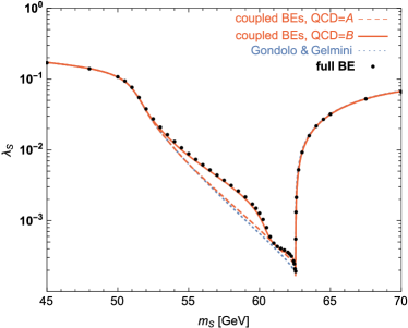
Let us first compute the relic density following the standard treatment adopted in the literature. To this end, we numerically solve Eq. (17) for a given set of parameters $(m_{S},\lambda_{S})$ and determine the resulting asymptotic value of $Y_{0}$. The blue dashed line in Fig. 1 shows the contour in this plane that results in $Y_{0}$ corresponding to a relic density of $\Omega h^{2}=0.1188$, c.f. Eq. (19). We restrict our discussion to values of $m_{S}$ in the kinematic range where $\langle\sigma v\rangle$ is enhanced due to the Higgs propagator given in Eq. (41), and the coupling $\lambda_{S}$ that results in the correct relic density is hence correspondingly decreased. This curve agrees with the corresponding result obtained in Ref. Cline et al. (2013).

For comparison, we show in the same figure the required value of $\lambda_{S}$ that results when instead solving the coupled system of Boltzmann equations (27) and (II.2), or when numerically solving the full Boltzmann equation as described in Section II.3 . Here, the solid (dashed) line shows the situation for the ‘B’ (‘A’) scenario for scatterings on quarks. Outside the resonance region, the coupled Boltzmann equations lead to identical results compared to the standard approach, indicating that kinetic decoupling indeed happens much later than chemical decoupling and that the assumption of local thermal equilibrium during chemical freeze-out thus is satisfied. For DM masses inside the resonance region, on the other hand, we can see that the two methods can give significantly different results, implying that this assumption must be violated. For the same reason, a smaller scattering rate (as in scenario ‘B’) leads to an even larger deviation from the standard scenario than the maximal scattering rate adopted in scenario ‘A’.

Figure 2: Temperatures at which DM number density and velocity dispersion (‘temperature’) start to deviate from their equlibrium values, defined for the purpose of this figure as $|Y-Y_{\rm eq}|=0.1\,Y_{\rm eq}$ and $|y-y_{\rm eq}|=0.1\,y_{\rm eq}$, respectively. These curves are based on solving the coupled system of Boltzmann equations (27) and (II.2), for the same parameter combinations as in Fig. 1 (resulting thus in the correct relic density).

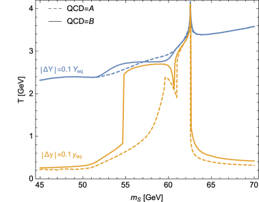
This interpretation is explicitly confirmed in Fig. 2, where we plot the temperatures at which the DM number density and temperature start to deviate from the equilibrium values: in the parameter range that we focus on here, kinetic decoupling happens indeed very close to chemical decoupling. The reason for this very early kinetic decoupling is straight-forward to understand as the result of a strongly suppressed momentum transfer rate $\gamma(T)$, compared to the annihilation rate, due to two independent effects: i) the small coupling $\lambda_{S}$ needed to satisfy the relic density requirement, without a corresponding resonant enhancement of $\gamma(T)$, and ii) the scattering rate being proportional to the Yukawa coupling squared, which favours scattering with Boltzmann-suppressed heavy fermions. We note that the latter point also explains the relatively large difference between the two extreme quark scattering scenarios used here for illustration (in scenario ‘B’, the largest Yukawa couplings do not contribute to the scattering).

Figure 3: The impact of the improved treatment of the kinetic decoupling on the relic density for parameter points that would satisfy the relic density constraint in the standard approach (dotted line in Fig. 1), both for the minimal (solid) and maximal (dashed) scenario for scattering with quarks. The numerical result (‘full BE’) implements minimal quark scattering; note that this does not take into account the effect of DM self-interactions (while the other curves are consistent with assuming a maximal self-scattering rate). The green dashed curve shows the impact of implementing the elastic scattering term in the highly non-relativistic limit, c.f. Eq. (5).

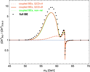
In order to emphasize the importance of our improved treatment of the decoupling history, we plot in Fig. 3 also the ratio of the resulting relic density to that of the standard approach (for parameter values satisfying the relic density constraint for the latter, i.e. corresponding to the blue dashed curve in Fig. 1). Let us stress that, compared to the observational uncertainty in this quantity of about 1 %, these corrections are by no means small even in the minimal scattering scenario ‘A’. In the same figure, we also compare our result for the coupled system of Boltzmann equations (27) and (II.2) to the full numerical solution of the Boltzmann equation in phase space, as described in Section II.3 (black dots). Before getting back to these results, let us briefly comment on the green dashed line in Fig. 3, which implements the highly non-relativistic scattering term $C_{\text{el}}$ of Eq. (5), and hence not the replacement (35) in Eq. (II.2) which we otherwise adopt as our default. Clearly, the impact of this choice is very limited for this approach. We note that the quantitative importance of the relativistic correction term proportional to $\langle p^{4}/E^{3}\rangle$ in Eq. (II.2) lies in the same ballpark, affecting the relic density by at most $\sim$$10\%$ in the region very close to the resonance (and below the percent-level elsewhere).

Figure 4: Phase space distributions and their evolution for a Scalar Singlet DM particle with $m_{S}=57$ GeV. Left panel: Unit normalized phase-space distributions $f_{n}(q)$ from our full numerical solution of the Boltzmann equation (red lines) and thermal equilibrium distributions $f^{\text{eq}}_{n}(q)$ (blue lines) at four different temperatures $x=m_{S}/T=$ 16 (solid), 20 (dashed), 25 (dot-dashed) and 50 (dotted). The equilibrium distributions $f^{\text{eq}}_{n}$ are Maxwell-Boltzmann distributions evaluated at the ‘temperatures’ $T_{\chi}$, as defined in Eqs. (20, 21). The bottom part shows the fractional deviation from the respective thermal distribution $f_{n}(q)/f_{n}^{\text{eq}}(q)$. Right panel: The evolution of $Y$ (blue) and $y$ (yellow), assuming a Higgs-scalar coupling that leads to the correct relic density in the standard approach (dotted line in Fig. 1). We show these curves for the standard case (dotted lines), the approach using coupled Boltzmann equations (dashed) and the full numerical result (solid). The thin gray line indicates the asymptotic value of $Y$ corresponding to the observed relic density.

In Appendix A we discuss in depth the time evolution of both the coupled Boltzmann equations and the full phase-space density in the resonance region. Let us here just mention that the characteristic features of the curves displayed in Figs. 2 and 3 can indeed all more or less directly be understood in terms of the highly enhanced annihilation rate in a relatively narrow kinematic region around the resonance, $\sqrt{s}\sim m_{h}\pm\Gamma_{h}$. As the full numerical solution reveals, furthermore, the shape of $f_{\chi}(p)$ can in some cases be quite different from the Maxwell-Boltzmann form (34) that is consistent with the coupled system of Boltzmann equations (27) and (II.2). Whether this has a noticeable impact on the resulting relic density (like for $m_{S}\sim 57$ GeV) or not (like for $m_{S}\sim m_{h}/2$) again mostly depends on whether or not the shape is affected for those momenta that can combine to $\sqrt{s}\sim m_{h}$ during chemical freeze-out.

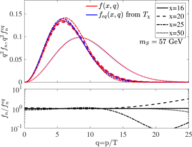
For illustration, we pick a DM mass of $m_{S}=57$ GeV and show in Fig. 4 the full phase-space distribution for a few selected values of $x$ (left panel) as well as the relevant evolution of $Y$ and $y$ (right panel). For models with DM masses in this range, the relatively large difference between full solution and coupled equations (as visible in Fig. 3) can mostly be understood in terms of the dip in the ratio of DM phase-space distributions at intermediate values of $q=p/T$ that starts to develop for $x\gtrsim 20$. Concretely, the fact that the actual distribution for those momenta is slightly suppressed compared to a distribution fully characterized only by its second moment, as in Eq. (34), causes the DM particles to annihilate less efficiently, $\langle\sigma v\rangle_{\mathrm{neq}}<\langle\sigma v\rangle$, because this is the momentum range probed by the resonance for these $x$ values. This in turn leads to the DM particles falling out of chemical equilibrium earlier, and hence a larger asymptotic value of $Y$. The reason for this momentum suppression to develop in the first place is also to be found in the particularly efficient annihilation close to the resonance, which leads to a depletion of DM particles with corresponding momenta because the scattering rate is no longer sufficiently large to redistribute the phase-space distribution to a thermal shape. We note that the bulk part of this effect is actually well captured by the coupled Boltzmann system, c.f. the dashed vs. solid lines in the right panel of Fig. 4. For further details, we refer again to Appendix A.

IV Discussion

From the above discussion, we have learned that very early kinetic decoupling is not just a theoretical possibility. It can appear in simple WIMP models, like the Scalar Singlet case, and affect the DM relic density in a significant way. We note that the size of the latter effect is, as expected, directly related to the size of the momentum exchange rate and hence to just how early kinetic decoupling happens compared to chemical decoupling. Let us stress that, from a general point of view, this is a much more important message connected to our choice of considering two scattering scenarios than the question of which of those scenarios is more realistic for the specific model we have studied here.

We have also seen that the coupled system of Boltzmann equations (27) and (II.2) provides a qualitatively very good description for the resulting DM abundance, see in particular Fig. 1, even though for high-precision results it seems mandatory to actually solve the full Boltzmann equation in phase space. As discussed in Appendix A, differences can arise when the true phase-space distribution is not of the Maxwellian form assumed in Eq. (34) – though the two methods can actually still give almost identical results for the relic abundance even when the two distribution differ vastly. The question of under which conditions the coupled system of equations provides an accurate description of the relic density is thus a somewhat subtle one, and requires a careful discussion of the velocity dependence of the annihilation term in the Boltzmann equation.

An exception to this general complication is a DM self-interaction rate large enough to force the DM distribution into the form given by Eq. (34) Feng et al. (2010a); Buckley and Fox (2010); Feng et al. (2010b); van den Aarssen et al. (2012) and hence render the coupled system of Boltzmann equations (27) and (II.2) exactly correct (up to, as discussed, corrections due to quantum statistics). Sizeable self-scattering rates can for example arise due to corresponding contact interactions, like the quartic coupling $\lambda_{SS}$ in the Scalar Singlet case, or by adding light mediators that couple to the DM particle (which was indeed the first time such a coupled system of Boltzmann equations was considered van den Aarssen et al. (2012), albeit in a different context). For the case of resonant annihilation, furthermore, the same resonance also mediates an enhanced self-interaction. For future work, it would hence be worthwhile to extend our numerical framework to even include those DM self-interaction processes. For the Scalar Singlet case, in particular, we expect that adding the process $SS\to h^{*}\to SS$ would bring all numerical results for the full Boltzmann equation – e.g. those shown in Fig. 3 – even closer to those resulting from the coupled system of Boltzmann equations.

Let us finally stress that both the coupled Boltzmann equations and the numerical setup that we have described here are very general, and can be used to consistently study early kinetic decoupling for a much larger range of models than the Scalar Singlet case. Obvious applications are other scenarios where resonant annihilation and/or annihilation to heavy final states is important in setting the relic abundance, see also Ref. Duch and Grzadkowski (2017). Further examples where the ratio of the scattering rate to the annihilation rate can be smaller than usual, hence potentially leading to early kinetic decoupling, include Sommerfeld-enhanced annihilation Dent et al. (2010); Zavala et al. (2010); Feng et al. (2010b); van den Aarssen et al. (2012) (if the light mediators are not abundant enough to take part in the scattering process) and annihilation to DM bound states Feng et al. (2009); von Harling and Petraki (2014). Quite in general, our methods provide a powerful means to check whether the DM particles are indeed in local thermal equilibrium with the heat bath around the time when their abundance freezes out – which is the usual assumption, though rarely explicitly tested, not only in WIMP-like scenarios but also when so-called semi-annihilations D’Eramo and Thaler (2010) are important in setting the relic density, when computing the relic abundance for modified expansion histories D’Eramo et al. (2017); Redmond and Erickcek (2017), or in scenarios that go beyond simple $2\to 2$ annihilation processes Hochberg et al. (2014, 2015); Kuflik et al. (2016).

V Conclusions

The standard way of calculating the thermal relic density of self-annihilating DM particles rests on the assumption of local thermal equilibrium during freeze-out, and that hence kinetic decoupling occurs much later than chemical decoupling. Here, we demonstrated for the first time that departure from kinetic equilibrium can instead happen much earlier, even simultaneously with the departure from chemical equilibrium.

By introducing a coupled system of equations for the DM number density and its ‘temperature’, or rather velocity dispersion, we improved the standard way of calculating the relic density in such cases. For an even higher accuracy in predicting the DM abundance, we also found a way of solving the full Boltzmann equation numerically. The latter approach has the additional advantage of obtaining the full phase-space distribution, rather than only the number density, which in particular allows to test in detail the assumption of a Maxwellian velocity distribution adopted in the standard approach. A numerical solver for the coupled system of Boltzmann equations, Eqs. (27, II.2), will be available in an upcoming version of DarkSUSY Bringmann et al. (2018) and our implemented solver for the full Boltzmann equation at the phase-space level, Eq. (38), will be released separately.

Applied to the simplest renormalizable WIMP model – the Scalar Singlet, extensively discussed in the literature – we somewhat surprisingly found that the relic abundance predicted in the standard approach can differ by up to an order of magnitude from the correct treatment presented in this paper. This is rather remarkable not only in view of the simplicity of this model, but also because the affected region in parameter space happens to coincide with the best-fit region resulting from most recent global scans. We thus expect our results to have a noticeable phenomenological impact, and that our treatment will prove useful also when applied to other examples of relic density calculations in cases where the standard assumption of local thermal equilibrium during freeze-out is not exactly satisfied.

Note added. While preparing this work, we became aware of a dedicated study on resonant DM annihilation Duch and Grzadkowski (2017), which also found that DM can kinetically decouple much earlier than usual in this case.

Acknowledgments.—

We thank Mateusz Duch, Joakim Edsjö, Bohdan Grza̧dkowski, Andreas Hohenegger and Ayuki Kamada for very useful conversations during the preparation of this work. We are also grateful to Tomohiro Abe for pointing out a previously missing factor of 4 in Eqs. (42,43), as well as our detailed discussions around the coupled system of Boltzmann equations (27,II.2). AH is supported by the University of Oslo through the Strategic Dark Matter Initiative (SDI). MG and T. Binder have received funding from the European Union’s Horizon 2020 research and innovation programme under grant agreement No 690575 and No 674896. T. Binder gratefully acknowledges financial support from the German Science Foundation (DFG RTG 1493).

Figure 5: Same as the left panel of Fig. 4 in the main text, but now for comparison for various DM masses $m_{S}=45,57,60.5,62,62.5,63$ GeV. Note that for cases where the equilibrium distributions appear to be missing in the top panels, it is just because it agrees very well with the actual phase-space distribution (as also visible in the fractional deviation plotted in the bottom panels).

Appendix A Phase-space density evolution of the Scalar Singlet

In Section III.2, we investigated the impact of our improved treatment of the Boltzmann equation on the expected DM relic abundance in the Scalar Singlet model. Here, we supplement this by discussing in some more detail the evolution of the DM phase-space density. The main focus of this discussion, however, will be a more thorough qualitative understanding of the specific features seen in Fig. 2 and Fig. 3, and the underlying interplay of chemical and early kinetic decoupling. Specifically, we can distinguish three mass regimes:

1. A regime with $53\,{\rm GeV}\lesssim m_{S}\lesssim 60.5$ GeV, which we will refer to as sub-resonant because $f_{\chi}$ starts to deviate from its equilibrium value, $f_{\chi,{\rm eq}}=\exp(-E/T)$, at a temperature where the typical DM momenta are too small to hit the resonance, i.e. $\sqrt{s}\lesssim m_{h}-\Gamma_{h}$. As a result, we have $\langle\sigma v\rangle_{\rm(neq)}<\langle\sigma v\rangle_{2,{\rm(neq)}}$ during the whole freeze-out process in this regime — this is because $p^{2}f_{\chi}(p)$ peaks at a higher value of $p$ than $f_{\chi}(p)$, which brings its bulk distribution closer to (or even on) the cross-section resonance.

2. A regime with $60.5\,{\rm GeV}\lesssim m_{S}\lesssim 62.5$ GeV that we will refer to as resonant. Here, we have $\langle\sigma v\rangle>\langle\sigma v\rangle_{2}$ around the time when the DM particles start to leave thermal equilibrium, because the larger mass combines with the relevant momenta to $s\sim m_{h}^{2}$. At slightly later times, on the other hand, still relevant in changing the DM abundance, the DM momenta have redshifted so much that we are back to a situation where typically $\sqrt{s}\lesssim m_{h}-\Gamma_{h}$ and hence $\langle\sigma v\rangle<\langle\sigma v\rangle_{2}$.

3. Finally, there is a super-resonant regime with $62.5\,{\rm GeV}\lesssim m_{S}\lesssim 65$ GeV, where decoupling occurs at such high temperatures that we have $\langle\sigma v\rangle>\langle\sigma v\rangle_{2}$ during the whole time it takes for $Y(x)$ to reach its asymptotic value (determining the relic density).

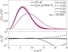
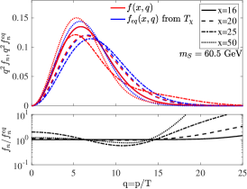
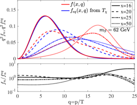
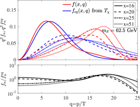
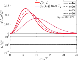
To help our discussion, let us look at a selection of benchmark points with Scalar Singlet masses $m_{S}=45,57,60.5,62,62.5,63$ GeV and coupling constants $\lambda_{S}(m_{S})$ that result in the correct relic density in the standard approach (dotted line in Fig. 1). In Fig. 5, we show the DM distribution function for these benchmark points that we find with our full numerical approach, for selected values of $x$, and in Fig. 6

Figure 6: Evolution of $Y(x)$ and $y(x)$, for the same DM masses as shown in Fig. 5.

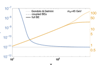
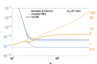
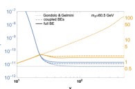
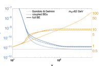
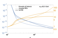
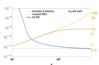
the full evolution of $Y(x)$ and $y(x)$ for the different approaches. These figures thus extend the information in Fig. 4 by covering a range of DM masses.

The first thing to note, as exemplified by the benchmark points with $m_{S}=45$ GeV and $m_{S}=63$ GeV, is that for masses sufficiently far away from the resonance we find a phase-space distribution which remains almost exactly Maxwellian in shape. For these points, we therefore find as expected a very good agreement for the evolution of $Y(x)$ and $y(x)$ when comparing the numerical solution and the coupled Boltzmann approach, as well as with $Y$ in the standard Gondolo & Gelmini setup (which assumes $T=T_{\chi}$). We note that this provides an important consistency check for both methods.

An example for a model in the sub-resonant region is the case with $m_{S}=57$ GeV, which we discussed in the main text. Here, the resonant annihilation depletes $f_{\chi}(q)$ for momenta just above the peak of the distribution, leading to a relative decrease with respect to a thermal distribution at these momenta, and hence a decrease in the DM velocity dispersion (aka ‘temperature’). This effect is visible in Fig. 5 starting with a slight suppression at $q\sim 8$ for the curve with $x=20$ (note that the relative enhancement at larger values of $q$ is not relevant for our discussion given that $f_{\chi}$ is already highly suppressed here), and results in the decrease in the evolution of $y$ seen in Fig. 6. The latter can also directly be understood from inspection of Eq. (II.2): in the sub-resonant regime we have $\langle\sigma v\rangle<\langle\sigma v\rangle_{2}$, which drives $y$ to smaller values after decoupling (with a strength proportional to $Y$ – which explains why the scattering term $\propto\gamma(T)$ can increase $y$ again, slightly, once the DM abundance has decreased sufficiently). A second effect of this depletion in $f_{\chi}(q)$ is that $\langle\sigma v\rangle_{\mathrm{neq}}$ decreases, which in turn leads to an earlier chemical decoupling and hence an increased relic density. The difference between the numerical and the coupled Boltzmann approach can in this case thus exclusively be understood as resulting from the slight offset in the $y(x)$ curves during the freeze-out (which in turn results from the fact that the scattering term is not strong enough to maintain an exact Maxwellian shape of $f_{\chi}(q)$ when the velocity dispersion decreases as explained above.)

As we increase the DM mass, we leave the sub-resonant regime and enter the resonant regime, with the transition point marked by the benchmark model with $m_{S}=60.5$ GeV. We note that this transition is also clearly visible in Fig. 2, as a sharp decrease in the temperature at which the DM velocity dispersion deviates from its equilibrium value. The origin of this feature is not an actual delay of kinetic decoupling, but that DM annihilation now starts to deplete $f_{\chi}(q)$ below the peak of the would-be Maxwellian distribution. This leads to an increase of the velocity dispersion, once equilibrium is left, rather than a decrease as in the sub-resonant regime. This effect is very clearly seen in Figs. 5 and 6, up to DM masses at the higher end of this regime, where the influence of the resonance starts to become less important because we have $\sqrt{s}\lesssim m_{h}+\Gamma_{h}$ only for DM momenta well below the peak of the phase-space distribution.

In the super-resonant regime with $m_{S}\gtrsim m_{h}/2$, finally, we have necessarily $\sqrt{s}\gtrsim m_{h}$. A resonantly enhanced annihilation rate is thus only possible for a very small portion of phase-space, with almost vanishing relative DM momenta. This implies not only that we always have $\langle\sigma v\rangle>\langle\sigma v\rangle_{2}$ in this regime, but also that the effect of the resonance rapidly becomes negligible.

Lastly, it is interesting to note that for $\sqrt{s}\gtrsim m_{h}$ the annihilation rate effectively features a $1/v^{2}$ velocity dependence. This is similar to resonant Sommerfeld-enhanced annihilation, which leads to a suppressed relic density after a prolonged freeze-out phase van den Aarssen et al. (2012). This can clearly be seen in the evolution of $Y(x)$ in Fig. 6, for $m_{S}\sim m_{h}/2$, where the differences between the numerical and the coupled Boltzmann approach are mostly due to the late-time differences in $y(x)$ – which in turn come about because of the rather significant differences in $f_{\chi}(q)$ at large values of $x$ (c.f. Fig. 5).

Appendix B Semi-relativistic kinetic theory

In this Appendix, we discuss how to generalize the highly non-relativistic elastic scattering term in Eq. (5) to incorporate the most important relativistic corrections needed for the numerical implementation of the full Boltzmann equation. Throughout, we refer to this result as ‘semi-relativistic’ scattering.

The starting point is to expand the full collision term $C_{\text{el}}$ in small momentum transfer compared to the typical DM momentum – similar to what is done in order to arrive at Eq. (5), but not only keeping lowest-order terms in $\mathbf{p}^{2}/m_{\chi}^{2}\sim T/m_{\chi}$. From this, we can derive a Fokker-Planck scattering operator in a relativistic form (for details, see Binder et al. (2016)):

$$C_{\mathrm{el}}\simeq\frac{E}{2}\nabla_{\mathbf{p}}\cdot{\Bigg{[}}\gamma(T,\mathbf{p})\left(ET\nabla_{\mathbf{p}}+\mathbf{p}\right)f_{\chi}{\Bigg{]}}\,.$$ (44)

Being a total divergence, this scattering operator manifestly respects number conservation, as it should. Another important property, which one can directly read off from the part inside the brackets, is that it features a stationary point given by the relativistic Maxwell-Boltzmann distribution,

$$f_{\chi}^{\text{eq}}\propto e^{-E/T}.$$ (45)

The non-relativistic limit of Eq. (44) gives the scattering operator (5), but in this limit the stationary point would instead be the non-relativistic version $f_{\chi}^{\text{eq}}\propto\exp[-p^{2}/(2m_{\chi}T)]$ — which would cause a problem in the full BE as this does not correspond to the actual equilibrium distribution fed into the annihilation term of Eq. (37).

In general, the momentum transfer rate $\gamma(T,\mathbf{p})$ in Eq. (44) depends on the DM momentum $\mathbf{p}$. However, the stationary point is independent of $\gamma$, which motivates us to restrict ourselves to the leading order term $\gamma(T)\equiv\gamma(T,\mathbf{0})$, neglecting any momentum dependence, and use the non-relativistic limit in Eq. (44) only to evaluate the momentum transfer rate $\gamma(T)$ as it appears in Eq. (6). To this order, we could thus also replace the leading $E$ in Eq. (44) by $m_{\chi}$; here, we choose to still keep it as it leads to a much more compact analytical form of the equation governing the DM temperature (see below). Explicitly performing the first partial derivative in $C_{\text{el}}$ then leads to the final form of our semi-relativistic Fokker-Planck operator as given by Eq. (8). This operator is our default choice for the numerical implementation of the full Boltzmann equation.

As already pointed out in Section II.3, it is mandatory for the full phase-space calculation to have a scattering operator with a fixpoint that matches the equilibrium distribution of Eq. (45) assumed in the annihilation term. For the coupled integrated Boltzmann system, on the other hand, this issue is fully addressed by using the relativistic temperature definition of Eq. (21) — rather than its non relativistic version typically adopted in the literature in the context of kinetic decoupling — because this automatically leads to the correct fixpoint $T_{\chi}=T$ for both the semi-relativistic Eq. (8) and, to the lowest order, for the non-relativistic version Eq. (5); see the discussion in Section II.2.

Another advantage of our semi-relativistic Fokker-Planck operator is that the differential equation for $T_{\chi}$, often quoted when discussing kinetic decoupling, takes a very simple form even beyond the highly non-relativistic limit. To see this, let us for the moment ignore the impact of annihilations, and take the second moment of the Boltzmann equation with this operator (using the relativistic definition of $T_{\chi}$). This leads to

$$\dot{T}_{\chi}+2\left(1-\frac{\langle p^{4}/E^{3}\rangle}{6T_{\chi}}\right)HT_{\chi}=$$ (46)

$$\gamma{\Bigg{[}}T\left(1-\frac{5}{6}\langle p^{2}/E^{2}\rangle+\frac{2}{6}\langle p^{4}/E^{4}\rangle\right)-T_{\chi}\left(1-\frac{\langle p^{4}/E^{3}\rangle}{6T_{\chi}}\right){\Bigg{]}}\,,$$

which of course is equivalent to Eq. (II.2) in the main text, when neglecting the annihilation terms and implementing the replacement given in Eq. (35). Let us repeat that the r.h.s. of the above equation only takes this particular form with our default choice of the semi-relativistic Fokker-Planck term, whereas the moment appearing on the left hand side is an exact result. This equation is in general not closed in terms of $T_{\chi}$. However, if we make the ansatz of a Maxwellian DM phase-space distribution, c.f. Eq. (34), we get a relation between the different momentum moments,

$$5\langle p^{2}/E^{2}\rangle-2\langle p^{4}/E^{4}\rangle={\langle p^{4}/E^{3}\rangle}/{T_{\chi}},$$ (47)

such that the differential equation closes in terms of $T_{\chi}$. Indeed, introducing

$$2(1-w)\equiv\frac{g_{\chi}}{3T_{\chi}n_{\chi}}\int\frac{d^{3}p}{(2\pi)^{3}}\,\frac{\mathbf{p}^{4}}{E^{3}}f_{\chi}(\mathbf{p})=\frac{\langle p^{4}/E^{3}\rangle}{3T_{\chi}}\,,$$ (48)

it takes a very simple form:

$$\dot{T}_{\chi}+2w(T_{\chi})HT_{\chi}=w(T_{\chi})\gamma(T)\left(T-T_{\chi}\right).$$ (49)

This generalizes the highly nonrelativistic result Bringmann and Hofmann (2007), for which $w\to 1$ and we hence find the familiar scaling $T_{\chi}\propto T^{2}$ after kinetic decoupling (i.e. when $\gamma\ll H$). In the ultra-relativistic limit, on the other hand, we have $w(T_{\chi})\rightarrow 1/2$ and the likewise familiar scaling of $T_{\chi}\propto T$ for relativistic particles. We note that in the region $x\gtrsim 10$ relevant for early kinetic decoupling, the correction to the non-relativistic limit is already sizeable; e.g. $w(x=10)\approx 0.8$.

References

- Hinshaw et al. (2013) G. Hinshaw et al. (WMAP), Astrophys. J. Suppl. 208, 19 (2013), arXiv:1212.5226 [astro-ph.CO] .
- Ade et al. (2016) P. A. R. Ade et al. (Planck), Astron. Astrophys. 594, A13 (2016), arXiv:1502.01589 [astro-ph.CO] .
- Bertone et al. (2005) G. Bertone, D. Hooper, and J. Silk, Phys. Rept. 405, 279 (2005), arXiv:hep-ph/0404175 [hep-ph] .
- Lee and Weinberg (1977) B. W. Lee and S. Weinberg, Phys. Rev. Lett. 39, 165 (1977).
- Hut (1977) P. Hut, Phys. Lett. B69, 85 (1977).
- Sato and Kobayashi (1977) K. Sato and M. Kobayashi, Prog. Theor. Phys. 58, 1775 (1977).
- Dicus et al. (1977) D. A. Dicus, E. W. Kolb, and V. L. Teplitz, Phys. Rev. Lett. 39, 168 (1977), [Erratum: Phys. Rev. Lett.39,973(1977)].
- Wolfram (1979) S. Wolfram, Phys. Lett. B82, 65 (1979).
- Gondolo and Gelmini (1991) P. Gondolo and G. Gelmini, Nucl. Phys. B360, 145 (1991).
- Edsjo and Gondolo (1997) J. Edsjo and P. Gondolo, Phys. Rev. D56, 1879 (1997), arXiv:hep-ph/9704361 [hep-ph] .
- Griest and Seckel (1991) K. Griest and D. Seckel, Phys. Rev. D43, 3191 (1991).
- Bringmann (2009) T. Bringmann, New J. Phys. 11, 105027 (2009), arXiv:0903.0189 [astro-ph.CO] .
- D’Agnolo et al. (2017) R. T. D’Agnolo, D. Pappadopulo, and J. T. Ruderman, Phys. Rev. Lett. 119, 061102 (2017), arXiv:1705.08450 [hep-ph] .
- Silveira and Zee (1985) V. Silveira and A. Zee, Phys. Lett. B161, 136 (1985).
- McDonald (1994) J. McDonald, Phys. Rev. D50, 3637 (1994), arXiv:hep-ph/0702143 [HEP-PH] .
- Burgess et al. (2001) C. P. Burgess, M. Pospelov, and T. ter Veldhuis, Nucl. Phys. B619, 709 (2001), arXiv:hep-ph/0011335 [hep-ph] .
- Kolb and Turner (1990) E. W. Kolb and M. S. Turner, Front. Phys. 69, 1 (1990).
- Bringmann and Hofmann (2007) T. Bringmann and S. Hofmann, JCAP 0704, 016 (2007), [Erratum: JCAP1603,no.03,E02(2016)], arXiv:hep-ph/0612238 [hep-ph] .
- Kasahara (2009) J. Kasahara, Neutralino dark matter: the mass of the smallest halo and the golden region, Ph.D. thesis, The University of Utah (2009).
- Gondolo et al. (2012) P. Gondolo, J. Hisano, and K. Kadota, Phys. Rev. D86, 083523 (2012), arXiv:1205.1914 [hep-ph] .
- Binder et al. (2016) T. Binder, L. Covi, A. Kamada, H. Murayama, T. Takahashi, and N. Yoshida, JCAP 1611, 043 (2016), arXiv:1602.07624 [hep-ph] .
- Bringmann et al. (2016) T. Bringmann, H. T. Ihle, J. Kersten, and P. Walia, Phys. Rev. D94, 103529 (2016), arXiv:1603.04884 [hep-ph] .
- Belanger et al. (2002) G. Belanger, F. Boudjema, A. Pukhov, and A. Semenov, Comput. Phys. Commun. 149, 103 (2002), arXiv:hep-ph/0112278 [hep-ph] .
- Gondolo et al. (2004) P. Gondolo, J. Edsjo, P. Ullio, L. Bergstrom, M. Schelke, et al., JCAP 0407, 008 (2004), arXiv:astro-ph/0406204 [astro-ph] .
- Belanger et al. (2007) G. Belanger, F. Boudjema, A. Pukhov, and A. Semenov, Comput. Phys. Commun. 176, 367 (2007), arXiv:hep-ph/0607059 [hep-ph] .
- Arbey and Mahmoudi (2010) A. Arbey and F. Mahmoudi, Comput. Phys. Commun. 181, 1277 (2010), arXiv:0906.0369 [hep-ph] .
- Belanger et al. (2014) G. Belanger, F. Boudjema, A. Pukhov, and A. Semenov, Comput. Phys. Commun. 185, 960 (2014), arXiv:1305.0237 [hep-ph] .
- Bringmann et al. (2018) T. Bringmann, J. Edsjö, P. Gondolo, P. Ullio, and L. Bergström, JCAP 1807, 033 (2018), arXiv:1802.03399 [hep-ph] .
- Bringmann et al. (2017) T. Bringmann et al. (The GAMBIT Dark Matter Workgroup), Eur. Phys. J. C77, 831 (2017), arXiv:1705.07920 [hep-ph] .
- van den Aarssen et al. (2012) L. G. van den Aarssen, T. Bringmann, and Y. C. Goedecke, Phys. Rev. D85, 123512 (2012), arXiv:1202.5456 [hep-ph] .
- Duch and Grzadkowski (2017) M. Duch and B. Grzadkowski, JHEP 09, 159 (2017), arXiv:1705.10777 [hep-ph] .
- Feng et al. (2010a) J. L. Feng, M. Kaplinghat, and H.-B. Yu, Phys. Rev. Lett. 104, 151301 (2010a), arXiv:0911.0422 [hep-ph] .
- Buckley and Fox (2010) M. R. Buckley and P. J. Fox, Phys. Rev. D81, 083522 (2010), arXiv:0911.3898 [hep-ph] .
- Feng et al. (2010b) J. L. Feng, M. Kaplinghat, and H.-B. Yu, Phys. Rev. D82, 083525 (2010b), arXiv:1005.4678 [hep-ph] .
- Yaguna (2009) C. E. Yaguna, JCAP 0903, 003 (2009), arXiv:0810.4267 [hep-ph] .
- Profumo et al. (2010) S. Profumo, L. Ubaldi, and C. Wainwright, Phys. Rev. D82, 123514 (2010), arXiv:1009.5377 [hep-ph] .
- Arina and Tytgat (2011) C. Arina and M. H. G. Tytgat, JCAP 1101, 011 (2011), arXiv:1007.2765 [astro-ph.CO] .
- Mambrini (2011) Y. Mambrini, Phys. Rev. D84, 115017 (2011), arXiv:1108.0671 [hep-ph] .
- Lerner and McDonald (2009) R. N. Lerner and J. McDonald, Phys. Rev. D80, 123507 (2009), arXiv:0909.0520 [hep-ph] .
- Herranen et al. (2015) M. Herranen, T. Markkanen, S. Nurmi, and A. Rajantie, Phys. Rev. Lett. 115, 241301 (2015), arXiv:1506.04065 [hep-ph] .
- Kahlhoefer and McDonald (2015) F. Kahlhoefer and J. McDonald, JCAP 1511, 015 (2015), arXiv:1507.03600 [astro-ph.CO] .
- Profumo et al. (2007) S. Profumo, M. J. Ramsey-Musolf, and G. Shaughnessy, JHEP 08, 010 (2007), arXiv:0705.2425 [hep-ph] .
- Barger et al. (2009) V. Barger, P. Langacker, M. McCaskey, M. Ramsey-Musolf, and G. Shaughnessy, Phys. Rev. D79, 015018 (2009), arXiv:0811.0393 [hep-ph] .
- Cline and Kainulainen (2013) J. M. Cline and K. Kainulainen, JCAP 1301, 012 (2013), arXiv:1210.4196 [hep-ph] .
- Djouadi et al. (2012) A. Djouadi, O. Lebedev, Y. Mambrini, and J. Quevillon, Phys. Lett. B709, 65 (2012), arXiv:1112.3299 [hep-ph] .
- Cheung et al. (2012) K. Cheung, Y.-L. S. Tsai, P.-Y. Tseng, T.-C. Yuan, and A. Zee, JCAP 1210, 042 (2012), arXiv:1207.4930 [hep-ph] .
- Endo and Takaesu (2015) M. Endo and Y. Takaesu, Phys. Lett. B743, 228 (2015), arXiv:1407.6882 [hep-ph] .
- Djouadi et al. (2013) A. Djouadi, A. Falkowski, Y. Mambrini, and J. Quevillon, Eur. Phys. J. C73, 2455 (2013), arXiv:1205.3169 [hep-ph] .
- Cline et al. (2013) J. M. Cline, K. Kainulainen, P. Scott, and C. Weniger, Phys. Rev. D88, 055025 (2013), [Erratum: Phys. Rev.D92,no.3,039906(2015)], arXiv:1306.4710 [hep-ph] .
- Urbano and Xue (2015) A. Urbano and W. Xue, JHEP 03, 133 (2015), arXiv:1412.3798 [hep-ph] .
- He and Tandean (2016) X.-G. He and J. Tandean, JHEP 12, 074 (2016), arXiv:1609.03551 [hep-ph] .
- Escudero et al. (2016) M. Escudero, A. Berlin, D. Hooper, and M.-X. Lin, JCAP 1612, 029 (2016), arXiv:1609.09079 [hep-ph] .
- Goudelis et al. (2009) A. Goudelis, Y. Mambrini, and C. Yaguna, JCAP 0912, 008 (2009), arXiv:0909.2799 [hep-ph] .
- Craig et al. (2016) N. Craig, H. K. Lou, M. McCullough, and A. Thalapillil, JHEP 02, 127 (2016), arXiv:1412.0258 [hep-ph] .
- Han et al. (2016) H. Han, J. M. Yang, Y. Zhang, and S. Zheng, Phys. Lett. B756, 109 (2016), arXiv:1601.06232 [hep-ph] .
- Ko and Yokoya (2016) P. Ko and H. Yokoya, JHEP 08, 109 (2016), arXiv:1603.04737 [hep-ph] .
- Beniwal et al. (2016) A. Beniwal, F. Rajec, C. Savage, P. Scott, C. Weniger, M. White, and A. G. Williams, Phys. Rev. D93, 115016 (2016), arXiv:1512.06458 [hep-ph] .
- Cuoco et al. (2016) A. Cuoco, B. Eiteneuer, J. Heisig, and M. Krämer, JCAP 1606, 050 (2016), arXiv:1603.08228 [hep-ph] .
- Athron et al. (2017a) P. Athron et al. (GAMBIT), Eur. Phys. J. C77, 784 (2017a), [Addendum: Eur. Phys. J.C78,no.2,98(2018)], arXiv:1705.07908 [hep-ph] .
- Athron et al. (2017b) P. Athron et al. (GAMBIT), Eur. Phys. J. C77, 568 (2017b), arXiv:1705.07931 [hep-ph] .
- Patrignani et al. (2016) C. Patrignani et al. (Particle Data Group), Chin. Phys. C40, 100001 (2016).
- Dittmaier et al. (2011) S. Dittmaier et al. (LHC Higgs Cross Section Working Group), (2011), 10.5170/CERN-2011-002, arXiv:1101.0593 [hep-ph] .
- Boyanovsky et al. (2006) D. Boyanovsky, H. J. de Vega, and D. J. Schwarz, Ann. Rev. Nucl. Part. Sci. 56, 441 (2006), arXiv:hep-ph/0602002 [hep-ph] .
- Drees et al. (2015) M. Drees, F. Hajkarim, and E. R. Schmitz, JCAP 1506, 025 (2015), arXiv:1503.03513 [hep-ph] .
- Dent et al. (2010) J. B. Dent, S. Dutta, and R. J. Scherrer, Phys. Lett. B687, 275 (2010), arXiv:0909.4128 [astro-ph.CO] .
- Zavala et al. (2010) J. Zavala, M. Vogelsberger, and S. D. M. White, Phys. Rev. D81, 083502 (2010), arXiv:0910.5221 [astro-ph.CO] .
- Feng et al. (2009) J. L. Feng, M. Kaplinghat, H. Tu, and H.-B. Yu, JCAP 0907, 004 (2009), arXiv:0905.3039 [hep-ph] .
- von Harling and Petraki (2014) B. von Harling and K. Petraki, JCAP 1412, 033 (2014), arXiv:1407.7874 [hep-ph] .
- D’Eramo and Thaler (2010) F. D’Eramo and J. Thaler, JHEP 06, 109 (2010), arXiv:1003.5912 [hep-ph] .
- D’Eramo et al. (2017) F. D’Eramo, N. Fernandez, and S. Profumo, JCAP 1705, 012 (2017), arXiv:1703.04793 [hep-ph] .
- Redmond and Erickcek (2017) K. Redmond and A. L. Erickcek, Phys. Rev. D96, 043511 (2017), arXiv:1704.01056 [hep-ph] .
- Hochberg et al. (2014) Y. Hochberg, E. Kuflik, T. Volansky, and J. G. Wacker, Phys. Rev. Lett. 113, 171301 (2014), arXiv:1402.5143 [hep-ph] .
- Hochberg et al. (2015) Y. Hochberg, E. Kuflik, H. Murayama, T. Volansky, and J. G. Wacker, Phys. Rev. Lett. 115, 021301 (2015), arXiv:1411.3727 [hep-ph] .
- Kuflik et al. (2016) E. Kuflik, M. Perelstein, N. R.-L. Lorier, and Y.-D. Tsai, Phys. Rev. Lett. 116, 221302 (2016), arXiv:1512.04545 [hep-ph] .