The effect of the spatial domain in FANOVA models with ARH(1) error term

Javier Álvarez-Liébana1 and M. Dolores Ruiz–Medina1
Summary

Functional Analysis of Variance (FANOVA) from Hilbert-valued correlated data with spatial rectangular or circular supports is analyzed, when Dirichlet conditions are assumed on the boundary. Specifically, a Hilbert-valued fixed effect model with error term defined from an Autoregressive Hilbertian process of order one (ARH(1) process) is considered, extending the formulation given in Ruiz-Medina (2016). A new statistical test is also derived to contrast the significance of the functional fixed effect parameters. The Dirichlet conditions established at the boundary affect the dependence range of the correlated error term. While the rate of convergence to zero of the eigenvalues of the covariance kernels, characterizing the Gaussian functional error components, directly affects the stability of the generalized least-squares parameter estimation problem. A simulation study and a real-data application related to fMRI analysis are undertaken to illustrate the performance of the parameter estimator and statistical test derived.

Published in Statistics and Its Interface, 10, pp. 607-628. DOI: doi.org/10.4310/SII.2017.v10.n4.a7

1 Department of Statistics and O. R., University of Granada, Spain.

E-mail: javialvaliebana@ugr.es

Key words: ARH(1) error term; boundary value problems; Cram´er-Wold Theorem; functional analysis of variance; linear functional tests; fMRI data.

1 Introduction

In the last few decades, functional data analysis techniques have grown significantly given the new technologies available, in particular, in the field of medicine (see, for instance, Sorensen et al. [2013]). High–dimensional data, which are functional in nature, are generated, for example, from measurements in time, over spatial grids or images with many pixels (e.g., data on electrical activity of the heart, data on electrical activity along the scalp, data reconstructed from medical imaging, expression profiles in genetics and genomics, monitoring of continuity activity through accelerometers, etc). Effective experimental design and modern functional statistics have led to recent advances in medical imaging, improving, in particular, the study of human brain function (see, for example, Delzell et al. [2012]). Magnetic Resonance Imaging (MRI) data have been analysed with different aims. For example, we refer to the studies related with cortical thickness (see Lerch and Evans [2005]), where magnetic resonance imaging data are analysed to detect the spatial locations of the surface of the brain, where the cortical thickness is correlated with an independent variable, such as age or gender (see also Shaw et al. [2006]). Cortical thickness is usually previously smoothed along the surface of the brain (see Chung et al. [2005]). Thus, it can be considered as a functional random variable with spatial circular support. In general, the following linear model is considered, for cortical thickness Yi(s)subscript𝑌𝑖𝑠Y_{i}(s) on subjects i=1,,n,𝑖1𝑛i=1,\dots,n,:

Yi(𝐬)=𝒙i𝜷(𝐬)+Zi(𝐬)σi(𝐬),𝐬S,formulae-sequencesubscript𝑌𝑖𝐬subscript𝒙𝑖𝜷𝐬subscript𝑍𝑖𝐬subscript𝜎𝑖𝐬𝐬𝑆Y_{i}(\mathbf{s})=\boldsymbol{x}_{i}\boldsymbol{\beta}(\mathbf{s})+Z_{i}(\mathbf{s})\sigma_{i}(\mathbf{s}),\quad\mathbf{s}\in S, (1)

where 𝒙isubscript𝒙𝑖\boldsymbol{x}_{i} is a vector of known p𝑝p regressors, and for each 𝐬S,𝐬𝑆\mathbf{s}\in S, with S𝑆S denoting the surface of the brain, parameter 𝜷(𝐬)𝜷𝐬\boldsymbol{\beta}(\mathbf{s}) is an unknown p𝑝p–vector of regression coefficients. The errors {Z1,,Zn}subscript𝑍1subscript𝑍𝑛\left\{Z_{1},\dots,Z_{n}\right\} are independent zero-mean Gaussian random fields. In Taylor and Worsley [2007], this model is also considered to detect how the regressors are related to the data at spatial location 𝐬,𝐬\mathbf{s}, by testing contrasts in 𝜷(𝐬),𝜷𝐬\boldsymbol{\beta}(\mathbf{s}), for 𝐬S.𝐬𝑆\mathbf{s}\in S. The approach presented in this paper allows the formulation of model (1) in a functional (Hilbert–valued) framework, incorporating possible correlations between subjects, due to genetic characteristics, breed, geographic location, etc.

The statistical analysis of functional magnetic resonance image (fMRI) data has also generated an important activity in research about brain activity, where the functional statistical approach implemented in this paper could lead to important spatio–temporal analysis improvements. It is well–known that fMRI techniques have been developed to address the unobserved effect of scanner noise in studies of the auditory cortex. A penalized likelihood approach to magnetic resonance image reconstruction is presented in Bulaevskaya and Oehlert [2007]. A new approach which incorporates the spatial information from neighbouring voxels, as well as temporal correlation within each voxel, which makes use of regional kriging is derived in Christensen and Yetkin [2005]. Conditional autoregressive and Markov random field modelling involves some restrictions in the characterization of spatially contiguous effect regions, and, in general, in the representation of the spatial dependence between spatially connected voxels (see, for example, Banerjee et al. [2004], Besag [1986]). Multiscale adaptive regression models assume spatial independence to construct a weighted likelihood parameter estimate. At each scale, the weights determine the amount of information that observations in a neighborhood voxel provides on the parameter vector to be estimated at a given voxel, under the assumption of independence between the conditional distributions of the responses at the neighborhood voxels, for each scale. The weights are sequentially computed through different scales, for adaptively update of the parameter estimates and test statistics (see, for example, Li et al. [2011]).

In Zhu et al. [2012], a multivariate varying coefficient model is considered for neuroimaging data, under a mixed effect approach, to reflect dependence within–curve and between–curve, in the case where coefficients are one–parameter functions, although extension to higher dimension is straightforward. The approach presented in this paper adopts a functional framework to analyse multivariate varying coefficient models in higher dimensions (two–dimensional design points), under the framework of multivariate fixed effect models in Hilbert spaces. Namely, the response is a multivariate functional random variable reflecting dependence within-surface (between voxels), and between-surface (between different times), with Hilbert–valued multivariate Gaussian distribution. Hence, the varying coefficients are estimated from the application of an extended version of generalized least–squares estimation methodology, in the multivariate Hilbert–valued context (see Ruiz-Medina [2016]), while, in Zhu et al. [2012], local linear regression is applied to estimate the coefficient functions. The dependence structure of the functional response is estimated here from the moment–based parameter estimation of the ARH(1) error term (see Bosq [2000]). In Zhu et al. [2012], local linear regression technique is employed to estimate the random effects, reflecting dependence structure in the varying coefficient mixed effect model. An extended formulation of the varying coefficient model considered in Zhu et al. [2012] is given in Zhu et al. [2014], combining a univariate measurement mixed effect model, a jumping surface model, and a functional component analysis model. In the approach presented in this paper, we have combined a nonparametric surface model with a multivariate functional principal component approach in the ARH(1) framework. Thus, a continuous spatial variation of the fMRI response is assumed, incorporating temporal and spatial correlations (across voxels), with an important dimension reduction in the estimation of the varying coefficient functions.

The above–referred advances in medicine are supported by the extensive literature on linear models in function spaces developed in parallel in the last few decades. We particularly refer to the functional linear regression context (see, for example, Cai and Hall [2006], Cardot et al. [2003], Cardot and Sarda [2011], Chiou et al. [2004], Crambes et al. [2009], Cuevas et al. [2002], Ferraty et al. [2013], Kokoszka et al. [2008], among others). See also Bosq [2000, 2007], Ruiz-Medina [2011, 2012], in the functional time series context, and Ferraty and Vieu [2006, 2011] in the functional nonparametric regression framework. Functional Analysis of Variance (FANOVA) techniques for high–dimensional data with a functional background have played a crucial role, within the functional linear model literature as well. Related work has been steadily growing (see, for example, Angelini et al. [2003], Dette and Derbort [2001], Gu [2002], Huang [1998], Kaufman and Sain [2010], Kaziska [2011], Lin [2000], Ramsay and Silverman [2005], Spitzner et al. [2003], Stone et al. [1997], Wahba et al. [1995]). The paper Ruiz-Medina [2016] extends the results in Zoglat [2008] from the L2([0,1])superscript𝐿201L^{2}([0,1])–valued context to the separable Hilbert–valued space framework, and from the case of independent homocedastic error components to the correlated heteroscedastic case. In the context of hypothesis testing from functional data, tests of significance based on wavelet thresholding are formulated in Fan [1996], exploiting the sparsity of the signal representation in the wavelet domain, for dimension reduction. A maximum likelihood ratio based test is suggested for functional variance components in mixed–effect FANOVA models in Guo [2002]. From classical ANOVA tests, an asymptotic approach is derived in Cuevas et al. [2004], for studying the equality of the functional means from k𝑘k independent samples of functional data. The testing problem for mixed–effect functional analysis of variance models is addressed in Abramovich and Angelini [2006], Abramovich et al. [2004], developing asymptotically optimal (minimax) testing procedures for the significance of functional global trend, and the functional fixed effects. The wavelet transform of the data is again used in the implementation of this approach (see also Antoniadis and Sapatinas [2007]). Recently, in the context of functional data defined by curves, considering the L2superscript𝐿2L^{2}–norm, an up–to–date overview of hypothesis testing methods for functional data analysis is provided in Zhang [2013], including functional ANOVA, functional linear models with functional responses, heteroscedastic ANOVA for functional data, and hypothesis tests for the equality of covariance functions, among other related topics.

In this paper, the model formulated in Ruiz-Medina [2016] is extended to the case where the error term is an ARH(1) process. Furthermore, an alternative test to contrast the significance of the functional fixed effect parameters is formulated, based on a sharp form of the Cramér–Wold’s Theorem derived in Cuesta-Albertos et al. [2007], for Gaussian measures on a separable Hilbert space. The simulation study undertaken illustrates the effect of the boundary conditions and the geometry of the domain on the spatial dependence range of the functional vector error term. Specifically, in that simulations, we consider the case where the Gaussian error components satisfy a stochastic partial differential equation, given in terms of a fractional power of the Dirichlet negative Laplacian operator. The autocovariance and cross–covariance operators of the functional error components are then defined in terms of the eigenvectors of the Dirichlet negative Laplacian operator. The eigenvectors of the Dirichlet negative Laplacian operator vanish continuously at the boundary, in the case of the regular domains studied (the rectangle, disk and circular sector), with decay velocity determined by the boundary conditions and the geometry of the domain. Thus, the boundary conditions and the geometry of the domain directly affect the dependence range of the error components, determined by the rate of convergence to zero of the Dirichlet negative Laplacian eigenvectors at the boundary. The influence of the truncation order is studied as well, since the rate of convergence to zero of the eigenvalues of the spatial covariance kernels, that define the matrix covariance operator of the error term, could affect the stability of the generalized least–squares estimation problem addressed here. Furthermore, in the fMRI data problem considered, the presented functional fixed effect model, with ARH(1) error term, is fitted. In that case, the temporal dependence range of the error term is controlled by the ARH(1) dynamics, while the spatial dependence range is controlled by the boundary conditions. Thus, the performance of the functional least–squares estimator and the functional significance test introduced in this paper is illustrated in both cases, the simulation study and the real–data example considered. A comparative study with the classical approach presented in Worsley et al. [2002] is also achieved for the fMRI data set analysed (freely available at http://www.math.mcgill.ca/keith/fmristat/).

The outline of this paper is as follows. The functional fixed effect model with ARH(1) error term is formulated in Appendix 2. The main results obtained on generalized least–squares estimation of the Hilbert–valued vector of fixed effect parameters, and the functional analysis of variance are also collected in this appendix. Linear hypothesis testing is derived in Appendix 3. The results obtained from the simulation study undertaken are displayed in Appendix 4. Functional statistical analysis of fMRI data is given in Appendix 5. Conclusions and open research lines are provided in Appendix 6. Finally, the Supplementary Material in Appendix 7 introduces the required preliminary elements on eigenvectors and eigenvalues of the Dirichlet negative Laplacian operator on the rectangle, disk and circular sector.

2 Multivariate Hilbert–valued fixed effect model with ARH(1) error term

This section provides the extended formulation of the multivariate Hilbert–valued fixed effect model studied in Ruiz-Medina [2016], to the case where the correlated functional components of the error term satisfy an ARH(1) state equation. In that formulation, compactly supported non–separable autocovariance and cross–covariance kernels are considered for the functional error components, extending the separable case studied in Ruiz-Medina [2016].

Denote by H𝐻H a real separable Hilbert space with the inner product ,H,subscript𝐻\left\langle\cdot,\cdot\right\rangle_{H}, and the associated norm H.\|\cdot\|_{H}. Let us first introduce the multivariate Hilbert–valued fixed effect model with ARH(1) error term

𝐘()=𝐗𝜷()+𝜺(),𝐘𝐗𝜷𝜺\mathbf{Y}\left(\cdot\right)=\mathbf{X}\boldsymbol{\beta}\left(\cdot\right)+\boldsymbol{\varepsilon}\left(\cdot\right), (2)

where 𝐗𝐗\mathbf{X} is a real-valued n×p𝑛𝑝n\times p matrix, the fixed effect design matrix,

𝜷()=[β1(),,βp()]THp𝜷superscriptsubscript𝛽1subscript𝛽𝑝𝑇superscript𝐻𝑝\boldsymbol{\beta}(\cdot)=[\beta_{1}(\cdot),\dots,\beta_{p}(\cdot)]^{T}\in H^{p}

represents the vector of fixed effect parameters,

𝐘()=[Y1(),,Yn()]T𝐘superscriptsubscript𝑌1subscript𝑌𝑛𝑇\mathbf{Y}(\cdot)=[Y_{1}(\cdot),\dots,Y_{n}(\cdot)]^{T}

is the Hnsuperscript𝐻𝑛H^{n}-valued Gaussian response, with E{𝐘}=𝐗𝜷E𝐘𝐗𝜷{\rm E}\left\{\mathbf{Y}\right\}=\mathbf{X}\boldsymbol{\beta}. The Hnsuperscript𝐻𝑛H^{n}-valued error term

𝜺()=[ε1(),,εn()]T𝜺superscriptsubscript𝜀1subscript𝜀𝑛𝑇\boldsymbol{\varepsilon}(\cdot)=[\varepsilon_{1}(\cdot),\dots,\varepsilon_{n}(\cdot)]^{T}

is assumed to be an ARH(1) process on the basic probability space (Ω,𝒜,𝒫)Ω𝒜𝒫(\Omega,\mathcal{A},\mathcal{P}); i.e., a stationary in time Hilbert–valued Gaussian process satisfying (see Bosq [2000])

εm()=ρ(εm1)()+νm(),m,formulae-sequencesubscript𝜀𝑚𝜌subscript𝜀𝑚1subscript𝜈𝑚𝑚\varepsilon_{m}\left(\cdot\right)=\rho\left(\varepsilon_{m-1}\right)\left(\cdot\right)+\nu_{m}\left(\cdot\right),\quad m\in\mathbb{Z}, (3)

where E{εm}=0,Esubscript𝜀𝑚0{\rm E}\left\{\varepsilon_{m}\right\}=0, for each m,𝑚m\in\mathbb{Z}, and ρ𝜌\rho denotes the autocorrelation operator of the error process ε,𝜀\varepsilon, which belongs to the space of bounded linear operators on H.𝐻H. Here, ν={νm,m}𝜈subscript𝜈𝑚𝑚\nu=\left\{\nu_{m},\ m\in\mathbb{Z}\right\} is assumed to be a Gaussian strong white noise; i.e., ν𝜈\nu is a Hilbert–valued zero–mean stationary process, with independent and identically distributed components in time, and with σ2=E{νmH2}<,superscript𝜎2Esuperscriptsubscriptnormsubscript𝜈𝑚𝐻2\sigma^{2}={\rm E}\left\{\|\nu_{m}\|_{H}^{2}\right\}<\infty, for all m.𝑚m\in\mathbb{Z}. Thus, in (2), the components of the vector error term [ε1(),,εn()]Tsuperscriptsubscript𝜀1subscript𝜀𝑛𝑇[\varepsilon_{1}(\cdot),\dots,\varepsilon_{n}(\cdot)]^{T} corresponding to observations at times t1,,tn,subscript𝑡1subscript𝑡𝑛t_{1},\dots,t_{n}, obey the functional state equation (3), under suitable conditions on the point spectrum of the autocorrelation operator ρ𝜌\rho. Hence, the non–null functional entries of the matrix covariance operator 𝐑𝜺𝜺subscript𝐑𝜺𝜺\mathbf{R}_{\boldsymbol{\varepsilon}\boldsymbol{\varepsilon}} of

𝜺()=[ε1(),,εn()]T𝜺superscriptsubscript𝜀1subscript𝜀𝑛𝑇\boldsymbol{\varepsilon}(\cdot)=[\varepsilon_{1}(\cdot),\dots,\varepsilon_{n}(\cdot)]^{T}

are then constituted by the elements located at the three main diagonals. Specifically,

E{εiεj}=R1,if ji=1,E{εiεj}=R1,if ij=1,formulae-sequenceEtensor-productsubscript𝜀𝑖subscript𝜀𝑗subscript𝑅1formulae-sequenceif 𝑗𝑖1formulae-sequenceEtensor-productsubscript𝜀𝑖subscript𝜀𝑗superscriptsubscript𝑅1if 𝑖𝑗1{\rm E}\left\{\varepsilon_{i}\otimes\varepsilon_{j}\right\}=R_{1},\quad\text{if }j-i=1,\quad{\rm E}\left\{\varepsilon_{i}\otimes\varepsilon_{j}\right\}=R_{1}^{*},\quad\text{if }i-j=1,

and

E{εiεi}=R0,if i=j,formulae-sequenceEtensor-productsubscript𝜀𝑖subscript𝜀𝑖subscript𝑅0if 𝑖𝑗{\rm E}\left\{\varepsilon_{i}\otimes\varepsilon_{i}\right\}=R_{0},\quad\text{if }i=j,

where R1subscript𝑅1R_{1} and R1superscriptsubscript𝑅1R_{1}^{*} denote, respectively, the cross–covariance operator and its adjoint for the ARH(1) process ε={εi,i},𝜀subscript𝜀𝑖𝑖\varepsilon=\left\{\varepsilon_{i},\ i\in\mathbb{Z}\right\}, and R0subscript𝑅0R_{0} represents its autocovariance operator. Note that, in this appendix, it is assumed that ρ𝜌\rho is sufficiently regular. In particular, ρ𝜌\rho is such that ρ2(H)0similar-to-or-equalssubscriptnormsuperscript𝜌2𝐻0\|\rho^{2}\|_{\mathcal{L}(H)}\simeq 0.

Equivalently, the matrix covariance operator 𝐑𝜺𝜺subscript𝐑𝜺𝜺\mathbf{R}_{\boldsymbol{\varepsilon}\boldsymbol{\varepsilon}} is given by

𝐑𝜺𝜺subscript𝐑𝜺𝜺\displaystyle\mathbf{R}_{\boldsymbol{\varepsilon}\boldsymbol{\varepsilon}} =\displaystyle= E{[ε1(),,εn()]T[ε1(),,εn()]}Esuperscriptsubscript𝜀1subscript𝜀𝑛𝑇subscript𝜀1subscript𝜀𝑛\displaystyle{\rm E}\left\{\left[\varepsilon_{1}(\cdot),\dots,\varepsilon_{n}(\cdot)\right]^{T}\left[\varepsilon_{1}(\cdot),\dots,\varepsilon_{n}(\cdot)\right]\right\} (7)
=\displaystyle= (E{ε1ε1}E{ε1εn}E{εnε1}E{εnεn})Etensor-productsubscript𝜀1subscript𝜀1Etensor-productsubscript𝜀1subscript𝜀𝑛Etensor-productsubscript𝜀𝑛subscript𝜀1Etensor-productsubscript𝜀𝑛subscript𝜀𝑛\displaystyle\left(\begin{array}[]{ccc}{\rm E}\left\{\varepsilon_{1}\otimes\varepsilon_{1}\right\}&\ldots&{\rm E}\left\{\varepsilon_{1}\otimes\varepsilon_{n}\right\}\\ \vdots&\ddots&\vdots\\ {\rm E}\left\{\varepsilon_{n}\otimes\varepsilon_{1}\right\}&\ldots&{\rm E}\left\{\varepsilon_{n}\otimes\varepsilon_{n}\right\}\end{array}\right)
similar-to-or-equals\displaystyle\simeq (R0R10H0H0H0H0HR1R0R10H0H0H0H0H0H0H0HR1R0R10H0H0H0H0HR1R0),subscript𝑅0subscript𝑅1subscript0𝐻subscript0𝐻subscript0𝐻subscript0𝐻subscript0𝐻superscriptsubscript𝑅1subscript𝑅0subscript𝑅1subscript0𝐻subscript0𝐻subscript0𝐻subscript0𝐻subscript0𝐻subscript0𝐻subscript0𝐻subscript0𝐻superscriptsubscript𝑅1subscript𝑅0subscript𝑅1subscript0𝐻subscript0𝐻subscript0𝐻subscript0𝐻subscript0𝐻superscriptsubscript𝑅1subscript𝑅0\displaystyle\left(\begin{array}[]{cccccccc}R_{0}&R_{1}&0_{H}&0_{H}&\ldots&0_{H}&0_{H}&0_{H}\\ R_{1}^{*}&R_{0}&R_{1}&0_{H}&\ldots&0_{H}&0_{H}&0_{H}\\ \vdots&\vdots&\vdots&\vdots&\ddots&\vdots&\vdots&\vdots\\ 0_{H}&0_{H}&0_{H}&0_{H}&\ldots&R_{1}^{*}&R_{0}&R_{1}\\ 0_{H}&0_{H}&0_{H}&0_{H}&\ldots&0_{H}&R_{1}^{*}&R_{0}\\ \end{array}\right), (13)

where 0Hsubscript0𝐻0_{H} denotes the approximation by zero in the corresponding operator norm, given the conditions imposed on ρ𝜌\rho.

In the space =Hn,superscript𝐻𝑛\mathcal{H}=H^{n}, we consider the inner product

𝐟,𝐠Hn=i=1nfi,giH,𝐟,𝐠Hn.formulae-sequencesubscript𝐟𝐠superscript𝐻𝑛superscriptsubscript𝑖1𝑛subscriptsubscript𝑓𝑖subscript𝑔𝑖𝐻𝐟𝐠superscript𝐻𝑛\langle\mathbf{f},\mathbf{g}\rangle_{H^{n}}=\displaystyle\sum_{i=1}^{n}\langle f_{i},g_{i}\rangle_{H},\leavevmode\nobreak\ \quad\mathbf{f},\mathbf{g}\in H^{n}.

It is well–known that the autocovariance operator R0subscript𝑅0R_{0} of an ARH(1) process is in the trace class (see [Bosq, 2000, pp. 27–36]). Therefore, it admits a diagonal spectral decomposition

R0=k=1λkϕkϕk,subscript𝑅0superscriptsubscript𝑘1tensor-productsubscript𝜆𝑘subscriptitalic-ϕ𝑘subscriptitalic-ϕ𝑘R_{0}=\displaystyle\sum_{k=1}^{\infty}\lambda_{k}\phi_{k}\otimes\phi_{k},

in terms of a complete orthogonal eigenvector system {ϕk,k1},subscriptitalic-ϕ𝑘𝑘1\left\{\phi_{k},\ k\geq 1\right\}, defining in H𝐻H a resolution of the identity k=1ϕkϕksuperscriptsubscript𝑘1tensor-productsubscriptitalic-ϕ𝑘subscriptitalic-ϕ𝑘\displaystyle\sum_{k=1}^{\infty}\phi_{k}\otimes\phi_{k}. Here, for each k1,𝑘1k\geq 1, λk=λk(R0)subscript𝜆𝑘subscript𝜆𝑘subscript𝑅0\lambda_{k}=\lambda_{k}(R_{0}) is the k𝑘k–th eigenvalue of R0,subscript𝑅0R_{0}, with R0(ϕk)=λk(R0)ϕk.subscript𝑅0subscriptitalic-ϕ𝑘subscript𝜆𝑘subscript𝑅0subscriptitalic-ϕ𝑘R_{0}\left(\phi_{k}\right)=\lambda_{k}(R_{0})\phi_{k}. The following series expansion then holds, in the mean–square sense:

εi=k=1εi,ϕkHϕk=k=1λkηk(i)ϕk,i=1,,n,formulae-sequencesubscript𝜀𝑖superscriptsubscript𝑘1subscriptsubscript𝜀𝑖subscriptitalic-ϕ𝑘𝐻subscriptitalic-ϕ𝑘superscriptsubscript𝑘1subscript𝜆𝑘subscript𝜂𝑘𝑖subscriptitalic-ϕ𝑘𝑖1𝑛\varepsilon_{i}=\displaystyle\sum_{k=1}^{\infty}\left\langle\varepsilon_{i},\phi_{k}\right\rangle_{H}\phi_{k}=\displaystyle\sum_{k=1}^{\infty}\sqrt{\lambda_{k}}\eta_{k}(i)\phi_{k},\quad i=1,\dots,n,

where ηk(i)=1λkεi,ϕkH,subscript𝜂𝑘𝑖1subscript𝜆𝑘subscriptsubscript𝜀𝑖subscriptitalic-ϕ𝑘𝐻\eta_{k}(i)=\frac{1}{\sqrt{\lambda_{k}}}\langle\varepsilon_{i},\phi_{k}\rangle_{H}, for k1𝑘1k\geq 1 and i.𝑖i\in\mathbb{N}.


The following assumption is made:


Assumption A0. The standard Gaussian random variable sequences {ηk(i),k1,i},formulae-sequencesubscript𝜂𝑘𝑖𝑘1𝑖\{\eta_{k}(i),\ k\geq 1,\leavevmode\nobreak\ i\in\mathbb{N}\}, with, for each k1,𝑘1k\geq 1,

λkηk(i)=εi,ϕkH,subscript𝜆𝑘subscript𝜂𝑘𝑖subscriptsubscript𝜀𝑖subscriptitalic-ϕ𝑘𝐻\sqrt{\lambda_{k}}\eta_{k}(i)=\left\langle\varepsilon_{i},\phi_{k}\right\rangle_{H},

for every i,𝑖i\in\mathbb{N}, satisfy the following orthogonality condition, for every i,j,𝑖𝑗i,j\in\mathbb{N},

E{ηk(i)ηp(j)}=δk,p,k,p,formulae-sequenceEsubscript𝜂𝑘𝑖subscript𝜂𝑝𝑗subscript𝛿𝑘𝑝𝑘𝑝{\rm E}\left\{\eta_{k}(i)\eta_{p}(j)\right\}=\delta_{k,p},\quad k,p\in\mathbb{N},

where δ𝛿\delta denotes the Kronecker delta function, and

R1subscript𝑅1\displaystyle R_{1} =\displaystyle= k=1λk(R1)ϕkϕk,R1=k=1λk(R1)ϕkϕk.superscriptsubscript𝑘1tensor-productsubscript𝜆𝑘subscript𝑅1subscriptitalic-ϕ𝑘subscriptitalic-ϕ𝑘superscriptsubscript𝑅1superscriptsubscript𝑘1tensor-productsubscript𝜆𝑘superscriptsubscript𝑅1subscriptitalic-ϕ𝑘subscriptitalic-ϕ𝑘\displaystyle\sum_{k=1}^{\infty}\lambda_{k}(R_{1})\phi_{k}\otimes\phi_{k},\quad R_{1}^{*}=\sum_{k=1}^{\infty}\lambda_{k}(R_{1}^{*})\phi_{k}\otimes\phi_{k}.

Under Assumption A0, the computation of the generalized least–squares estimator of [β1(),,βp()]Tsuperscriptsubscript𝛽1subscript𝛽𝑝𝑇[\beta_{1}(\cdot),\dots,\beta_{p}(\cdot)]^{T} is achieved by projection into the orthogonal basis of eigenvectors {ϕk,k1}subscriptitalic-ϕ𝑘𝑘1\left\{\phi_{k},\ k\geq 1\right\} of the autocovariance operator R0subscript𝑅0R_{0} of the ARH(1) process ε={εi,i}.𝜀subscript𝜀𝑖𝑖\varepsilon=\left\{\varepsilon_{i},\ i\in\mathbb{Z}\right\}. Denote by 𝚽superscript𝚽\boldsymbol{\Phi}^{*} the projection operator into the eigenvector system {ϕk,k1},subscriptitalic-ϕ𝑘𝑘1\left\{\phi_{k},\ k\geq 1\right\}, acting on a vector function 𝐟=Hn𝐟superscript𝐻𝑛\mathbf{f}\in\mathcal{H}=H^{n} as follows:

𝚽(𝐟)superscript𝚽𝐟\displaystyle\boldsymbol{\Phi}^{*}\left(\mathbf{f}\right) =\displaystyle= {𝚽k(𝐟),k1}={(f1,ϕk,,fn,ϕk)T,k1}superscriptsubscript𝚽𝑘𝐟𝑘1superscriptsubscript𝑓1subscriptitalic-ϕ𝑘subscript𝑓𝑛subscriptitalic-ϕ𝑘𝑇𝑘1\displaystyle\left\{\boldsymbol{\Phi}_{k}^{*}\left(\mathbf{f}\right),\ k\geq 1\right\}=\left\{\left(\langle f_{1},\phi_{k}\rangle,\dots,\langle f_{n},\phi_{k}\rangle\right)^{T},\ k\geq 1\right\} (14)
=\displaystyle= {(fk1,,fkn)T,k1}={𝐟kT,k1},superscriptsubscript𝑓𝑘1subscript𝑓𝑘𝑛𝑇𝑘1superscriptsubscript𝐟𝑘𝑇𝑘1\displaystyle\left\{\left(f_{k1},\dots,f_{kn}\right)^{T},\ k\geq 1\right\}=\left\{\mathbf{f}_{k}^{T},\ k\geq 1\right\},

where 𝚽𝚽=𝐈𝐝=Hn,𝚽superscript𝚽subscript𝐈𝐝superscript𝐻𝑛\boldsymbol{\Phi}\boldsymbol{\Phi}^{*}=\mathbf{Id}_{\mathcal{H}=H^{n}}, with

𝚽({𝐟kT,k1})=(k=1fk1ϕk,,k=1fknϕk)T.𝚽superscriptsubscript𝐟𝑘𝑇𝑘1superscriptsuperscriptsubscript𝑘1subscript𝑓𝑘1subscriptitalic-ϕ𝑘superscriptsubscript𝑘1subscript𝑓𝑘𝑛subscriptitalic-ϕ𝑘𝑇\boldsymbol{\Phi}\left(\left\{\mathbf{f}_{k}^{T},\ k\geq 1\right\}\right)=\left(\displaystyle\sum_{k=1}^{\infty}f_{k1}\phi_{k},\ldots,\displaystyle\sum_{k=1}^{\infty}f_{kn}\phi_{k}\right)^{T}.

For 𝐀={Ai,j}i=1,,nj=1,,n𝐀superscriptsubscriptsubscript𝐴𝑖𝑗𝑖1𝑛𝑗1𝑛\mathbf{A}=\left\{A_{i,j}\right\}_{i=1,\ldots,n}^{j=1,\ldots,n} be a matrix operator such that, for each i,j=1,,n,formulae-sequence𝑖𝑗1𝑛i,j=1,\dots,n, its functional entries are given by

Ai,j=k=1γkijϕkϕksubscript𝐴𝑖𝑗superscriptsubscript𝑘1tensor-productsubscript𝛾𝑘𝑖𝑗subscriptitalic-ϕ𝑘subscriptitalic-ϕ𝑘A_{i,j}=\displaystyle\sum_{k=1}^{\infty}\gamma_{kij}\phi_{k}\otimes\phi_{k}

with k=1γkij2<.superscriptsubscript𝑘1superscriptsubscript𝛾𝑘𝑖𝑗2\displaystyle\sum_{k=1}^{\infty}\gamma_{kij}^{2}<\infty. The following identities are straightforward:

𝚽𝐀𝚽superscript𝚽𝐀𝚽\displaystyle\boldsymbol{\Phi}^{*}\mathbf{A}\boldsymbol{\Phi} =\displaystyle= {𝚪k,k1},𝚽({𝚪k,k1})𝚽=𝐀,subscript𝚪𝑘𝑘1𝚽subscript𝚪𝑘𝑘1superscript𝚽𝐀\displaystyle\left\{\boldsymbol{\Gamma}_{k},\ k\geq 1\right\},\quad\boldsymbol{\Phi}\left(\left\{\boldsymbol{\Gamma}_{k},\ k\geq 1\right\}\right)\boldsymbol{\Phi}^{*}=\mathbf{A}, (15)

where, for each k1,𝑘1k\geq 1, the entries of 𝚪ksubscript𝚪𝑘\boldsymbol{\Gamma}_{k} are Γkij=γkij,subscriptΓ𝑘𝑖𝑗subscript𝛾𝑘𝑖𝑗\Gamma_{kij}=\gamma_{kij}, for i,j=1,,n.formulae-sequence𝑖𝑗1𝑛i,j=1,\dots,n.


Applying (14)–(15), we directly obtain

𝚽𝐑𝜺𝜺𝚽superscript𝚽subscript𝐑𝜺𝜺𝚽\displaystyle\boldsymbol{\Phi}^{*}\mathbf{R}_{\boldsymbol{\varepsilon}\boldsymbol{\varepsilon}}\boldsymbol{\Phi} =\displaystyle= {𝚲k,k1},𝚽𝐑𝜺𝜺1𝚽={𝚲k1,k1},subscript𝚲𝑘𝑘1superscript𝚽superscriptsubscript𝐑𝜺𝜺1𝚽superscriptsubscript𝚲𝑘1𝑘1\displaystyle\left\{\boldsymbol{\Lambda}_{k},\ k\geq 1\right\},\quad\boldsymbol{\Phi}^{*}\mathbf{R}_{\boldsymbol{\varepsilon}\boldsymbol{\varepsilon}}^{-1}\boldsymbol{\Phi}=\left\{\boldsymbol{\Lambda}_{k}^{-1},\ k\geq 1\right\},
𝐑𝜺𝜺1(𝐟,𝐠)superscriptsubscript𝐑𝜺𝜺1𝐟𝐠\displaystyle\mathbf{R}_{\boldsymbol{\varepsilon}\boldsymbol{\varepsilon}}^{-1}\left(\mathbf{f},\mathbf{g}\right) =\displaystyle= 𝚽𝐑𝜺𝜺1𝚽(𝚽𝐟,𝚽𝐠)=𝐟,𝐠𝐑𝜺𝜺1=k=1𝐟kT𝚲k1𝐠k,𝐟,𝐠𝐑𝜺𝜺1/2(Hn),formulae-sequencesuperscript𝚽superscriptsubscript𝐑𝜺𝜺1𝚽superscript𝚽𝐟superscript𝚽𝐠subscript𝐟𝐠superscriptsubscript𝐑𝜺𝜺1superscriptsubscript𝑘1superscriptsubscript𝐟𝑘𝑇superscriptsubscript𝚲𝑘1subscript𝐠𝑘𝐟𝐠superscriptsubscript𝐑𝜺𝜺12superscript𝐻𝑛\displaystyle\boldsymbol{\Phi}^{*}\mathbf{R}_{\boldsymbol{\varepsilon}\boldsymbol{\varepsilon}}^{-1}\boldsymbol{\Phi}\left(\boldsymbol{\Phi}^{*}\mathbf{f},\boldsymbol{\Phi}^{*}\mathbf{g}\right)=\langle\mathbf{f},\mathbf{g}\rangle_{\mathbf{R}_{\boldsymbol{\varepsilon}\boldsymbol{\varepsilon}}^{-1}}=\displaystyle\sum_{k=1}^{\infty}\mathbf{f}_{k}^{T}\boldsymbol{\Lambda}_{k}^{-1}\mathbf{g}_{k},\quad\mathbf{f},\leavevmode\nobreak\ \mathbf{g}\in\mathbf{R}_{\boldsymbol{\varepsilon}\boldsymbol{\varepsilon}}^{1/2}\left(H^{n}\right),
𝐟𝐑𝜺𝜺12superscriptsubscriptnorm𝐟superscriptsubscript𝐑𝜺𝜺12\displaystyle\|\mathbf{f}\|_{\mathbf{R}_{\boldsymbol{\varepsilon}\boldsymbol{\varepsilon}}^{-1}}^{2} =\displaystyle= k=1𝐟kT𝚲k1𝐟k,𝐟𝐑𝜺𝜺1/2(Hn),superscriptsubscript𝑘1superscriptsubscript𝐟𝑘𝑇superscriptsubscript𝚲𝑘1subscript𝐟𝑘𝐟superscriptsubscript𝐑𝜺𝜺12superscript𝐻𝑛\displaystyle\displaystyle\sum_{k=1}^{\infty}\mathbf{f}_{k}^{T}\boldsymbol{\Lambda}_{k}^{-1}\mathbf{f}_{k},\quad\mathbf{f}\in\mathbf{R}_{\boldsymbol{\varepsilon}\boldsymbol{\varepsilon}}^{1/2}\left(H^{n}\right), (16)

where, for each k1𝑘1k\geq 1, 𝚲k=𝚽k𝐑𝜺𝜺𝚽ksubscript𝚲𝑘subscriptsuperscript𝚽𝑘subscript𝐑𝜺𝜺subscript𝚽𝑘\boldsymbol{\Lambda}_{k}=\boldsymbol{\Phi}^{*}_{k}\mathbf{R}_{\boldsymbol{\varepsilon}\boldsymbol{\varepsilon}}\boldsymbol{\Phi}_{k} is given by

𝚲k=[λk(R0)λk(R1)000λk(R1)λk(R0)λk(R1)00000λk(R1)λk(R0)],subscript𝚲𝑘delimited-[]subscript𝜆𝑘subscript𝑅0subscript𝜆𝑘subscript𝑅1000subscript𝜆𝑘superscriptsubscript𝑅1subscript𝜆𝑘subscript𝑅0subscript𝜆𝑘subscript𝑅100000subscript𝜆𝑘superscriptsubscript𝑅1subscript𝜆𝑘subscript𝑅0\boldsymbol{\Lambda}_{k}=\left[\begin{array}[]{cccccc}\lambda_{k}(R_{0})&\lambda_{k}(R_{1})&0&\dots&0&0\\ \lambda_{k}(R_{1}^{*})&\lambda_{k}(R_{0})&\lambda_{k}(R_{1})&\dots&0&0\\ \vdots&\vdots&\vdots&\ddots&\vdots&\vdots\\ 0&0&0&\dots&\lambda_{k}(R_{1}^{*})&\lambda_{k}(R_{0})\\ \end{array}\right], (17)

with 𝚲k1superscriptsubscript𝚲𝑘1\boldsymbol{\Lambda}_{k}^{-1} denoting its inverse matrix.


Remark 1

In Appendix 4, we restrict our attention to the functional error model studied in Ruiz-Medina [2016], considering the Hilbert–valued stochastic partial differential equation system framework. In that framework, matrices {𝚲k,k1},subscript𝚲𝑘𝑘1\left\{\boldsymbol{\Lambda}_{k},\ k\geq 1\right\}, are known, since they are defined from the eigenvalues of the differential operators involved in the equation system. Particularly, in that section, for each k1,𝑘1k\geq 1, matrix 𝚲ksubscript𝚲𝑘\boldsymbol{\Lambda}_{k} is considered to have entries ΛkijsubscriptΛ𝑘𝑖𝑗\Lambda_{kij} given by

ΛkijsubscriptΛ𝑘𝑖𝑗\displaystyle\Lambda_{kij} =\displaystyle= exp(|ij|λki+λkj),if ij,𝑖𝑗subscript𝜆𝑘𝑖subscript𝜆𝑘𝑗if 𝑖𝑗\displaystyle\exp\left(-\frac{|i-j|}{\lambda_{ki}+\lambda_{kj}}\right),\quad\text{if }i\neq j,
ΛkiisubscriptΛ𝑘𝑖𝑖\displaystyle\Lambda_{kii} =\displaystyle= λki=λk([fi(𝚫Dl)]2)=λk((𝚫D1)2(dγi))=[λk((𝚫D1))]2(dγi),subscript𝜆𝑘𝑖subscript𝜆𝑘superscriptdelimited-[]subscript𝑓𝑖subscript𝚫subscript𝐷𝑙2subscript𝜆𝑘superscriptsubscript𝚫subscript𝐷12𝑑subscript𝛾𝑖superscriptdelimited-[]subscript𝜆𝑘subscript𝚫subscript𝐷12𝑑subscript𝛾𝑖\displaystyle\lambda_{ki}=\lambda_{k}\left([f_{i}(-\boldsymbol{\Delta}_{D_{l}})]^{2}\right)=\lambda_{k}\left((-\boldsymbol{\Delta}_{D_{1}})^{-2(d-\gamma_{i})}\right)=\left[\lambda_{k}\left((-\boldsymbol{\Delta}_{D_{1}})\right)\right]^{-2(d-\gamma_{i})},

with

γi(0,d/2),i=1,,n,formulae-sequencesubscript𝛾𝑖0𝑑2𝑖1𝑛\gamma_{i}\in(0,d/2),\quad i=1,\dots,n,

and (𝚫Dl)subscript𝚫subscript𝐷𝑙(-\boldsymbol{\Delta}_{D_{l}}) representing the Dirichlet negative Laplacian operator on domain Dl,subscript𝐷𝑙D_{l}, for l=1𝑙1l=1 (the rectangle), l=2𝑙2l=2 (the disk) and l=3𝑙3l=3 (the circular sector). However, in practice, as shown in Appendix 5 in the analysis of fMRI data, matrices {𝚲k,k1},subscript𝚲𝑘𝑘1\left\{\boldsymbol{\Lambda}_{k},\ k\geq 1\right\}, are not known, and should be estimated from the data. Indeed, in that real–data example, we approximate the entries of {𝚲k,k1},subscript𝚲𝑘𝑘1\left\{\boldsymbol{\Lambda}_{k},\ k\geq 1\right\}, from the coefficients (eigenvalues and singular values), that define the diagonal spectral expansion of the empirical autocovariance R0^^subscript𝑅0\widehat{R_{0}} and cross covariance R1^^subscript𝑅1\widehat{R_{1}} operators, given by (see Bosq [2000])

R0^^subscript𝑅0\displaystyle\widehat{R_{0}} =\displaystyle= 1ni=1nεiεi,R1^=1n1i=1n1εiεi+1,R1^=1n1i=2nεiεi1.formulae-sequence1𝑛superscriptsubscript𝑖1𝑛tensor-productsubscript𝜀𝑖subscript𝜀𝑖^subscript𝑅11𝑛1superscriptsubscript𝑖1𝑛1tensor-productsubscript𝜀𝑖subscript𝜀𝑖1^superscriptsubscript𝑅11𝑛1superscriptsubscript𝑖2𝑛tensor-productsubscript𝜀𝑖subscript𝜀𝑖1\displaystyle\frac{1}{n}\sum_{i=1}^{n}\varepsilon_{i}\otimes\varepsilon_{i},\quad\widehat{R_{1}}=\frac{1}{n-1}\sum_{i=1}^{n-1}\varepsilon_{i}\otimes\varepsilon_{i+1},\quad\widehat{R_{1}^{\ast}}=\frac{1}{n-1}\sum_{i=2}^{n}\varepsilon_{i}\otimes\varepsilon_{i-1}. (19)

We also consider here the following semi–orthogonal condition for the non-square design matrix 𝐗::𝐗absent\mathbf{X}:


Assumption A1. The fixed effect design matrix 𝐗𝐗\mathbf{X} is a semi–orthogonal non–square matrix. That is,

𝐗T𝐗=𝐈𝐝p,𝐈𝐝pp×p.formulae-sequencesuperscript𝐗𝑇𝐗subscript𝐈𝐝𝑝subscript𝐈𝐝𝑝superscript𝑝𝑝\mathbf{X}^{T}\mathbf{X}=\mathbf{Id}_{p},\quad\mathbf{Id}_{p}\in\mathbb{R}^{p\times p}.

Remark 2

Assumption A1 implies (see Ruiz-Medina [2016])

k=1Tr(𝐗T𝚲k1𝐗)1<.superscriptsubscript𝑘1Trsuperscriptsuperscript𝐗𝑇superscriptsubscript𝚲𝑘1𝐗1\displaystyle\sum_{k=1}^{\infty}{\rm Tr}\left(\mathbf{X}^{T}\boldsymbol{\Lambda}_{k}^{-1}\mathbf{X}\right)^{-1}<\infty.

The generalized least–squares estimation of [β1(),,βp()]Tsuperscriptsubscript𝛽1subscript𝛽𝑝𝑇[\beta_{1}(\cdot),\ldots,\beta_{p}(\cdot)]^{T} is achieved by minimizing the loss quadratic function in the norm of the Reproducing Kernel Hilbert Space (RKHS norm). Note that, for an \mathcal{H}–valued zero–mean Gaussian random variable with autocovariance operator RZ,subscript𝑅𝑍R_{Z}, the RKHS of Z𝑍Z is defined by

(Z)=RZ1/2()𝑍superscriptsubscript𝑅𝑍12\mathcal{H}\left(Z\right)=R_{Z}^{1/2}\left(\mathcal{H}\right)

(see, for example, Prato and Zabczyk [2002]).

From equation (16) we get

E{𝐘𝐗𝜷𝑹𝜺𝜺12}=𝑹𝜺𝜺1(𝜺)(𝜺)=k=1E{𝜺k(𝜷k)𝚲k12}k=1E{𝜺k(𝜷k)𝚲^k12},Esuperscriptsubscriptnorm𝐘𝐗𝜷superscriptsubscript𝑹𝜺𝜺12superscriptsubscript𝑹𝜺𝜺1𝜺𝜺superscriptsubscript𝑘1Esuperscriptsubscriptnormsubscript𝜺𝑘subscript𝜷𝑘superscriptsubscript𝚲𝑘12similar-to-or-equalssuperscriptsubscript𝑘1Esuperscriptsubscriptnormsubscript𝜺𝑘subscript𝜷𝑘superscriptsubscript^𝚲𝑘12{\rm E}\left\{\|\mathbf{Y}-\mathbf{X}\boldsymbol{\beta}\|_{\boldsymbol{R}_{\boldsymbol{\varepsilon}\boldsymbol{\varepsilon}}^{-1}}^{2}\right\}=\boldsymbol{R}_{\boldsymbol{\varepsilon}\boldsymbol{\varepsilon}}^{-1}\left(\boldsymbol{\varepsilon}\right)\left(\boldsymbol{\varepsilon}\right)=\displaystyle\sum_{k=1}^{\infty}{\rm E}\left\{\|\boldsymbol{\varepsilon}_{k}\left(\boldsymbol{\beta}_{k}\right)\|_{\boldsymbol{\Lambda}_{k}^{-1}}^{2}\right\}\simeq\displaystyle\sum_{k=1}^{\infty}{\rm E}\left\{\|\boldsymbol{\varepsilon}_{k}\left(\boldsymbol{\beta}_{k}\right)\|_{\widehat{\boldsymbol{\Lambda}}_{k}^{-1}}^{2}\right\}, (20)

where, in the last identity, for each k1,𝑘1k\geq 1, matrix 𝚲^ksubscript^𝚲𝑘\widehat{\boldsymbol{\Lambda}}_{k} represents the empirical counterpart of 𝚲k,subscript𝚲𝑘\boldsymbol{\Lambda}_{k}, constructed from the eigenelements of R0^,^subscript𝑅0\widehat{R_{0}}, R1^^subscript𝑅1\widehat{R_{1}} and R1^,superscript^subscript𝑅1\widehat{R_{1}}^{\ast}, considered when R0subscript𝑅0R_{0} and R1subscript𝑅1R_{1} are unknown. Here,

𝜺=𝐘𝐗𝜷,𝜺k(𝜷k)=𝚽k(𝐘𝐗𝜷),k1.formulae-sequence𝜺𝐘𝐗𝜷formulae-sequencesubscript𝜺𝑘subscript𝜷𝑘superscriptsubscript𝚽𝑘𝐘𝐗𝜷𝑘1\boldsymbol{\varepsilon}=\mathbf{Y}-\mathbf{X}\boldsymbol{\beta},\quad\boldsymbol{\varepsilon}_{k}\left(\boldsymbol{\beta}_{k}\right)=\boldsymbol{\Phi}_{k}^{*}\left(\mathbf{Y}-\mathbf{X}\boldsymbol{\beta}\right),\quad k\geq 1.

The minimum of equation (20) is attached if, for each k1,𝑘1k\geq 1, the expectation

E{𝜺k(𝜷k)𝚲k12}Esuperscriptsubscriptnormsubscript𝜺𝑘subscript𝜷𝑘superscriptsubscript𝚲𝑘12{\rm E}\left\{\|\boldsymbol{\varepsilon}_{k}\left(\boldsymbol{\beta}_{k}\right)\|_{\boldsymbol{\Lambda}_{k}^{-1}}^{2}\right\}

is minimized, with, as before, 𝚲k1superscriptsubscript𝚲𝑘1\boldsymbol{\Lambda}_{k}^{-1} defining the inverse of matrix 𝚲ksubscript𝚲𝑘\boldsymbol{\Lambda}_{k} given in (17) (and approximated by 𝚲^k,subscript^𝚲𝑘\widehat{\boldsymbol{\Lambda}}_{k}, when R0subscript𝑅0R_{0} and R1subscript𝑅1R_{1} are unknown). That is,

𝜷^ksubscript^𝜷𝑘\displaystyle\widehat{\boldsymbol{\beta}}_{k} =\displaystyle= (βk1^,,βkp^)T=(𝐗T𝚲k1𝐗)1𝐗T𝚲k1𝐘k,superscript^subscript𝛽𝑘1^subscript𝛽𝑘𝑝𝑇superscriptsuperscript𝐗𝑇superscriptsubscript𝚲𝑘1𝐗1superscript𝐗𝑇superscriptsubscript𝚲𝑘1subscript𝐘𝑘\displaystyle\left(\widehat{\beta_{k1}},\dots,\widehat{\beta_{kp}}\right)^{T}=\left(\mathbf{X}^{T}\boldsymbol{\Lambda}_{k}^{-1}\mathbf{X}\right)^{-1}\mathbf{X}^{T}\boldsymbol{\Lambda}_{k}^{-1}\mathbf{Y}_{k},

and given by

(βk1~,,βkp~)T=(𝐗T𝚲^k1𝐗)1𝐗T𝚲^k1𝐘k,superscript~subscript𝛽𝑘1~subscript𝛽𝑘𝑝𝑇superscriptsuperscript𝐗𝑇superscriptsubscript^𝚲𝑘1𝐗1superscript𝐗𝑇superscriptsubscript^𝚲𝑘1subscript𝐘𝑘\left(\widetilde{\beta_{k1}},\dots,\widetilde{\beta_{kp}}\right)^{T}=\left(\mathbf{X}^{T}\widehat{\boldsymbol{\Lambda}}_{k}^{-1}\mathbf{X}\right)^{-1}\mathbf{X}^{T}\widehat{\boldsymbol{\Lambda}}_{k}^{-1}\mathbf{Y}_{k}, (21)

in the case where R0subscript𝑅0R_{0} and R1subscript𝑅1R_{1} are unknown. Here, 𝐘k=𝚽k(𝐘)subscript𝐘𝑘subscriptsuperscript𝚽𝑘𝐘\mathbf{Y}_{k}=\boldsymbol{\Phi}^{*}_{k}\left(\mathbf{Y}\right) is the vector of projections into ϕksubscriptitalic-ϕ𝑘\phi_{k} of the components of 𝐘,𝐘\mathbf{Y}, for each k1.𝑘1k\geq 1.

In the remaining of this section, we restrict our attention to the case where R0subscript𝑅0R_{0} and R1subscript𝑅1R_{1} are known. In that case,

𝜷^=𝚽({𝜷k^,k1})=(k=1βk1^ϕk,,k=1βkp^ϕk)T.^𝜷𝚽^subscript𝜷𝑘𝑘1superscriptsuperscriptsubscript𝑘1^subscript𝛽𝑘1subscriptitalic-ϕ𝑘superscriptsubscript𝑘1^subscript𝛽𝑘𝑝subscriptitalic-ϕ𝑘𝑇\widehat{\boldsymbol{\beta}}=\boldsymbol{\Phi}\left(\left\{\widehat{\boldsymbol{\beta}_{k}},\ k\geq 1\right\}\right)=\left(\displaystyle\sum_{k=1}^{\infty}\widehat{\beta_{k1}}\phi_{k},\dots,\displaystyle\sum_{k=1}^{\infty}\widehat{\beta_{kp}}\phi_{k}\right)^{T}.

The estimated response is then given by 𝐘^=𝐗𝜷^^𝐘𝐗^𝜷\widehat{\mathbf{Y}}=\mathbf{X}\widehat{\boldsymbol{\beta}}. Under Assumption A1,

E{k=1i=1pβ^ki2}Esuperscriptsubscript𝑘1superscriptsubscript𝑖1𝑝superscriptsubscript^𝛽𝑘𝑖2\displaystyle{\rm E}\left\{\displaystyle\sum_{k=1}^{\infty}\sum_{i=1}^{p}\widehat{\beta}_{ki}^{2}\right\} =\displaystyle= k=1Tr(𝐗T𝚲k1𝐗)1+𝜷Hp2<,superscriptsubscript𝑘1Trsuperscriptsuperscript𝐗𝑇superscriptsubscript𝚲𝑘1𝐗1subscriptsuperscriptnorm𝜷2superscript𝐻𝑝\displaystyle\displaystyle\sum_{k=1}^{\infty}{\rm Tr}(\mathbf{X}^{T}\boldsymbol{\Lambda}_{k}^{-1}\mathbf{X})^{-1}+\|\boldsymbol{\beta}\|^{2}_{H^{p}}<\infty, (22)

i.e., 𝜷^Hp^𝜷superscript𝐻𝑝\widehat{\boldsymbol{\beta}}\in H^{p} almost surely (see Ruiz-Medina [2016] for more details).


Remark 3

In the case where R0subscript𝑅0R_{0} and R1subscript𝑅1R_{1} are unknown, under the conditions assumed in [Bosq, 2000, Corollary 4.2, pp. 101–102], strong consistency of the empirical autocovariance operator R0^^subscript𝑅0\widehat{R_{0}} holds. Moreover, under the conditions assumed in [Bosq, 2000, Theorem 4.8, pp. 116–117], the empirical cross–covariance operator R0^^subscript𝑅0\widehat{R_{0}} is strongly–consistent. Therefore, the plug–in functional parameter estimator (21) satisfies (22), for n𝑛n sufficiently large.


The Functional Analysis of Variance of model in (2)–(3) can be achieved as described in Ruiz-Medina [2016]. Specifically, a linear transformation of the functional data should be considered, for the almost surely finiteness of the functional components of variance, in the following way:

𝐖𝐘=𝐖𝐗𝜷+𝐖𝜺,𝐖𝐘𝐖𝐗𝜷𝐖𝜺\mathbf{W}\mathbf{Y}=\mathbf{W}\mathbf{X}\boldsymbol{\beta}+\mathbf{W}\boldsymbol{\varepsilon}, (23)

where 𝐖𝐖\mathbf{W} is such that

𝐖=(k=1wk11ϕkϕkk=1wk1nϕkϕkk=1wkn1ϕkϕkk=1wknnϕkϕk),𝐖superscriptsubscript𝑘1tensor-productsubscript𝑤𝑘11subscriptitalic-ϕ𝑘subscriptitalic-ϕ𝑘superscriptsubscript𝑘1tensor-productsubscript𝑤𝑘1𝑛subscriptitalic-ϕ𝑘subscriptitalic-ϕ𝑘superscriptsubscript𝑘1tensor-productsubscript𝑤𝑘𝑛1subscriptitalic-ϕ𝑘subscriptitalic-ϕ𝑘superscriptsubscript𝑘1tensor-productsubscript𝑤𝑘𝑛𝑛subscriptitalic-ϕ𝑘subscriptitalic-ϕ𝑘\mathbf{W}=\left(\begin{array}[]{ccc}\displaystyle\sum_{k=1}^{\infty}w_{k11}\phi_{k}\otimes\phi_{k}&\dots&\displaystyle\sum_{k=1}^{\infty}w_{k1n}\phi_{k}\otimes\phi_{k}\\ \vdots&\ddots&\vdots\\ \displaystyle\sum_{k=1}^{\infty}w_{kn1}\phi_{k}\otimes\phi_{k}&\dots&\displaystyle\sum_{k=1}^{\infty}w_{knn}\phi_{k}\otimes\phi_{k}\end{array}\right),

and satisfies

k=1Tr(𝚲k1𝐖k)<.superscriptsubscript𝑘1Trsuperscriptsubscript𝚲𝑘1subscript𝐖𝑘\sum_{k=1}^{\infty}{\rm Tr}\left(\boldsymbol{\Lambda}_{k}^{-1}\mathbf{W}_{k}\right)<\infty. (24)

Here, for each k1,𝑘1k\geq 1, 𝚲ksubscript𝚲𝑘\boldsymbol{\Lambda}_{k} is defined in (17). The functional components of variance associated with the transformed model (23) are then given by

SST~~𝑆𝑆𝑇\displaystyle\widetilde{SST} =\displaystyle= 𝐖𝐘,𝐖𝐘R𝜺𝜺1=k=1𝐘kT𝐖kT𝚲k1𝐖k𝐘k,subscript𝐖𝐘𝐖𝐘superscriptsubscript𝑅𝜺𝜺1superscriptsubscript𝑘1superscriptsubscript𝐘𝑘𝑇superscriptsubscript𝐖𝑘𝑇superscriptsubscript𝚲𝑘1subscript𝐖𝑘subscript𝐘𝑘\displaystyle\langle\mathbf{W}\mathbf{Y},\mathbf{W}\mathbf{Y}\rangle_{R_{\boldsymbol{\varepsilon}\boldsymbol{\varepsilon}}^{-1}}=\displaystyle\sum_{k=1}^{\infty}\mathbf{Y}_{k}^{T}\mathbf{W}_{k}^{T}\boldsymbol{\Lambda}_{k}^{-1}\mathbf{W}_{k}\mathbf{Y}_{k},
SSE~~𝑆𝑆𝐸\displaystyle\widetilde{SSE} =\displaystyle= 𝐖(𝐘𝐘^),𝐖(𝐘𝐘^)R𝜺𝜺1=k=1(𝐌k𝐖k𝐘k)T𝚲k1𝐌k𝐖k𝐘k,subscript𝐖𝐘^𝐘𝐖𝐘^𝐘superscriptsubscript𝑅𝜺𝜺1superscriptsubscript𝑘1superscriptsubscript𝐌𝑘subscript𝐖𝑘subscript𝐘𝑘𝑇superscriptsubscript𝚲𝑘1subscript𝐌𝑘subscript𝐖𝑘subscript𝐘𝑘\displaystyle\langle\mathbf{W}\left(\mathbf{Y}-\widehat{\mathbf{Y}}\right),\mathbf{W}\left(\mathbf{Y}-\widehat{\mathbf{Y}}\right)\rangle_{R_{\boldsymbol{\varepsilon}\boldsymbol{\varepsilon}}^{-1}}=\displaystyle\sum_{k=1}^{\infty}\left(\mathbf{M}_{k}\mathbf{W}_{k}\mathbf{Y}_{k}\right)^{T}\boldsymbol{\Lambda}_{k}^{-1}\mathbf{M}_{k}\mathbf{W}_{k}\mathbf{Y}_{k},
SSR~~𝑆𝑆𝑅\displaystyle\widetilde{SSR} =\displaystyle= SST~SSE~.~𝑆𝑆𝑇~𝑆𝑆𝐸\displaystyle\widetilde{SST}-\widetilde{SSE}.

where 𝐌k=𝐈𝐝n×n𝐗(𝐗T𝚲k1𝐗)1𝐗T𝚲k1,subscript𝐌𝑘subscript𝐈𝐝𝑛𝑛𝐗superscriptsuperscript𝐗𝑇superscriptsubscript𝚲𝑘1𝐗1superscript𝐗𝑇superscriptsubscript𝚲𝑘1\mathbf{M}_{k}=\mathbf{Id}_{n\times n}-\mathbf{X}\left(\mathbf{X}^{T}\boldsymbol{\Lambda}_{k}^{-1}\mathbf{X}\right)^{-1}\mathbf{X}^{T}\boldsymbol{\Lambda}_{k}^{-1}, for each k1.𝑘1k\geq 1.

The statistics

F=SSR~SSE~,𝐹~𝑆𝑆𝑅~𝑆𝑆𝐸F=\frac{\widetilde{SSR}}{\widetilde{SSE}}, (25)

provides information on the relative magnitude between the empirical variability explained by the functional transformed model and the residual variability (see Appendix 4).

3 Significance test from the Cramér–Wold’s Theorem

In Ruiz-Medina [2016], a linear functional statistical test is formulated, with explicit definition of the probability distribution of the derived functional statistics under the null hypothesis:

H0:𝐊𝜷=𝐂,:subscript𝐻0𝐊𝜷𝐂H_{0}:\leavevmode\nobreak\ \mathbf{K}\boldsymbol{\beta}=\mathbf{C},

against

H1:𝐊𝜷𝐂,:subscript𝐻1𝐊𝜷𝐂H_{1}:\leavevmode\nobreak\ \mathbf{K}\boldsymbol{\beta}\neq\mathbf{C},

where 𝐂Hm𝐂superscript𝐻𝑚\mathbf{C}\in H^{m} and

𝐊:HpHm:𝐊superscript𝐻𝑝superscript𝐻𝑚\mathbf{K}:H^{p}\longrightarrow H^{m}

is a matrix operator such that its functional entries 𝐊={Kij}i=1,,mj=1,,p,𝐊superscriptsubscriptsubscript𝐾𝑖𝑗𝑖1𝑚𝑗1𝑝\mathbf{K}=\left\{K_{ij}\right\}_{i=1,\dots,m}^{j=1,\dots,p}, are given, for each f,gH,𝑓𝑔𝐻f,g\in H, by

Kij(f)(g)=k=1λk(Kij)ϕk,gHϕk,fH.subscript𝐾𝑖𝑗𝑓𝑔superscriptsubscript𝑘1subscript𝜆𝑘subscript𝐾𝑖𝑗subscriptsubscriptitalic-ϕ𝑘𝑔𝐻subscriptsubscriptitalic-ϕ𝑘𝑓𝐻K_{ij}\left(f\right)\left(g\right)=\displaystyle\sum_{k=1}^{\infty}\lambda_{k}\left(K_{ij}\right)\langle\phi_{k},g\rangle_{H}\langle\phi_{k},f\rangle_{H}.

In particular,

{(𝚽k𝐊𝚽k),k1}={𝐊k,k1}superscriptsubscript𝚽𝑘𝐊subscript𝚽𝑘𝑘1subscript𝐊𝑘𝑘1\left\{\left(\boldsymbol{\Phi}_{k}^{*}\mathbf{K}\boldsymbol{\Phi}_{k}\right),\ k\geq 1\right\}=\left\{\mathbf{K}_{k},\ k\geq 1\right\}

with

𝐊k=(λk(K11)λk(K1p)λk(Km1)λk(Kmp))m×p.subscript𝐊𝑘subscript𝜆𝑘subscript𝐾11subscript𝜆𝑘subscript𝐾1𝑝subscript𝜆𝑘subscript𝐾𝑚1subscript𝜆𝑘subscript𝐾𝑚𝑝superscript𝑚𝑝\mathbf{K}_{k}=\left(\begin{array}[]{ccc}\lambda_{k}\left(K_{11}\right)&\dots&\lambda_{k}\left(K_{1p}\right)\\ \vdots&\ddots&\vdots\\ \lambda_{k}\left(K_{m1}\right)&\dots&\lambda_{k}\left(K_{mp}\right)\end{array}\right)\in\mathbb{R}^{m\times p}.

At level α,𝛼\alpha, there exists a test ψ𝜓\psi given by:

ψ={1ifSH0(𝐘)>C(H0,α),0otherwise,𝜓cases1ifsubscript𝑆subscript𝐻0𝐘𝐶subscript𝐻0𝛼0otherwise,\psi=\left\{\begin{array}[]{l}1\quad\mbox{if}\quad S_{H_{0}}(\mathbf{Y})>C(H_{0},\alpha),\\ 0\quad\mbox{otherwise,}\\ \end{array}\right.

where

SH0(𝐘)=𝐊𝜷^𝐂,𝐊𝜷^𝐂=Hn.subscript𝑆subscript𝐻0𝐘subscript𝐊^𝜷𝐂𝐊^𝜷𝐂superscript𝐻𝑛S_{H_{0}}(\mathbf{Y})=\left\langle\mathbf{K}\widehat{\boldsymbol{\beta}}-\mathbf{C},\mathbf{K}\widehat{\boldsymbol{\beta}}-\mathbf{C}\right\rangle_{\mathcal{H}=H^{n}}.

The constant C(H0,α)𝐶subscript𝐻0𝛼C(H_{0},\alpha) is such that

𝒫{SH0(𝐘)>C(H0,α),𝐊𝜷=𝐂}=1𝒫{SH0(𝐘)C(H0,α),𝐊𝜷=𝐂}=1𝐅α=α,𝒫formulae-sequencesubscript𝑆subscript𝐻0𝐘𝐶subscript𝐻0𝛼𝐊𝜷𝐂1𝒫formulae-sequencesubscript𝑆subscript𝐻0𝐘𝐶subscript𝐻0𝛼𝐊𝜷𝐂1subscript𝐅𝛼𝛼\displaystyle\mathcal{P}\left\{S_{H_{0}}(\mathbf{Y})>C(H_{0},\alpha),\quad\mathbf{K}\boldsymbol{\beta}=\mathbf{C}\right\}=1-\mathcal{P}\left\{S_{H_{0}}(\mathbf{Y})\leq C(H_{0},\alpha),\leavevmode\nobreak\ \mathbf{K}\boldsymbol{\beta}=\mathbf{C}\right\}=1-\mathbf{F}_{\alpha}=\alpha,

where the probability distribution 𝐅𝐅\mathbf{F} on =Hnsuperscript𝐻𝑛\mathcal{H}=H^{n} has characteristic functional given in [Ruiz-Medina, 2016, Proposition 4, Eq. (66)].

Alternatively, as an application of [Cuesta-Albertos et al., 2007, Theorem 4.1], a multivariate version of the significance test formulated in Cuesta-Albertos and Febrero-Bande [2010] is considered here, for the fixed effect parameters (see, in particular, [Cuesta-Albertos and Febrero-Bande, 2010, Theorem 2.1]. Specifically, we consider

H0𝐡:𝐊𝜷(𝐡)=𝐂,:superscriptsubscript𝐻0𝐡𝐊𝜷𝐡𝐂H_{0}^{\mathbf{h}}:\leavevmode\nobreak\ \mathbf{K}\boldsymbol{\beta}(\mathbf{h})=\mathbf{C}, (26)

for 𝐡=(h,,h)p×1T𝐡subscriptsuperscript𝑇𝑝1\mathbf{h}=(h,\dots,h)^{T}_{p\times 1} defining a random vector in Hp,superscript𝐻𝑝H^{p}, with hh generated from a zero–mean Gaussian measure μ𝜇\mu in H,𝐻H, with trace covariance operator Rμsubscript𝑅𝜇R_{\mu} (see, for example, Prato and Zabczyk [2002]). Here,

𝜷(𝐡)=(β1,hH,,βp,hH)p×1T,𝜷𝐡subscriptsuperscriptsubscriptsubscript𝛽1𝐻subscriptsubscript𝛽𝑝𝐻𝑇𝑝1\boldsymbol{\beta}(\mathbf{h})=\left(\left\langle\beta_{1},h\right\rangle_{H},\dots,\left\langle\beta_{p},h\right\rangle_{H}\right)^{T}_{p\times 1},

𝐊𝐊\mathbf{K} is given by

𝐊=(110010101001)(p1)×p,𝐊110010101001superscript𝑝1𝑝\mathbf{K}=\left(\begin{array}[]{ccccc}1&-1&0&\dots&0\\ 1&0&-1&\dots&0\\ \vdots&\vdots&\vdots&\ddots&\vdots\\ 1&0&0&\dots&-1\end{array}\right)\in\mathbb{R}^{\left(p-1\right)\times p}, (27)

and 𝐂𝐂\mathbf{C} is a null (p1)×1𝑝11\left(p-1\right)\times 1 functional vector; i.e.,

𝐂=(0,0,,0)T(p1)×1.𝐂superscript000𝑇superscript𝑝11\mathbf{C}=\left(0,0,\dots,0\right)^{T}\in\mathbb{R}^{\left(p-1\right)\times 1}. (28)

From equations (27)–(28), for any (p×1)𝑝1\left(p\times 1\right)–dimensional functional random vector 𝐡=(h,,h)p×1T𝐡superscriptsubscript𝑝1𝑇\mathbf{h}=(h,\dots,h)_{p\times 1}^{T} generated from a Gaussian measure μ𝜇\mu on H,𝐻H, H0𝐡superscriptsubscript𝐻0𝐡H_{0}^{\mathbf{h}} can then be equivalently expressed as

H0𝐡:β1,hH=β2,hH==βp,hH.:superscriptsubscript𝐻0𝐡subscriptsubscript𝛽1𝐻subscriptsubscript𝛽2𝐻subscriptsubscript𝛽𝑝𝐻H_{0}^{\mathbf{h}}:\leavevmode\nobreak\ \left\langle\beta_{1},h\right\rangle_{H}=\left\langle\beta_{2},h\right\rangle_{H}=\dots=\left\langle\beta_{p},h\right\rangle_{H}. (29)

The test statistic to contrast (29) is defined as

T𝒉=(𝐊𝜷^(𝐡)𝐂)T(𝐊𝐐𝐡𝐊T)1(𝐊𝜷^(𝐡)𝐂),subscript𝑇𝒉superscript𝐊^𝜷𝐡𝐂𝑇superscriptsubscript𝐊𝐐𝐡superscript𝐊𝑇1𝐊^𝜷𝐡𝐂T_{\boldsymbol{h}}=\left(\mathbf{K}\widehat{\boldsymbol{\beta}}(\mathbf{h})-\mathbf{C}\right)^{T}\left(\mathbf{K}\mathbf{Q}_{\mathbf{h}}\mathbf{K}^{T}\right)^{-1}\left(\mathbf{K}\widehat{\boldsymbol{\beta}}(\mathbf{h})-\mathbf{C}\right), (30)

where 𝐊𝐊\mathbf{K} and 𝐂𝐂\mathbf{C} are respectively given in equations (27)–(28), and

𝐐𝐡subscript𝐐𝐡\displaystyle\mathbf{Q}_{\mathbf{h}} =\displaystyle= (𝐗T𝚲𝐡𝐗)1,𝜷^(𝐡)=(𝐗T𝚲𝐡1𝐗)1𝐗T𝚲𝐡1𝐘(𝐡),superscriptsuperscript𝐗𝑇subscript𝚲𝐡𝐗1^𝜷𝐡superscriptsuperscript𝐗𝑇superscriptsubscript𝚲𝐡1𝐗1superscript𝐗𝑇superscriptsubscript𝚲𝐡1𝐘𝐡\displaystyle(\mathbf{X}^{T}\boldsymbol{\Lambda}_{\mathbf{h}}\mathbf{X})^{-1},\quad\widehat{\boldsymbol{\beta}}(\mathbf{h})=\left(\mathbf{X}^{T}\boldsymbol{\Lambda}_{\mathbf{h}}^{-1}\mathbf{X}\right)^{-1}\mathbf{X}^{T}\boldsymbol{\Lambda}_{\mathbf{h}}^{-1}\mathbf{Y}(\mathbf{h}), (31)

with

𝐘(𝐡)=(Y1,hH,,Yn,hH).𝐘𝐡subscriptsubscript𝑌1𝐻subscriptsubscript𝑌𝑛𝐻\mathbf{Y}(\mathbf{h})=\left(\left\langle Y_{1},h\right\rangle_{H},\dots,\left\langle Y_{n},h\right\rangle_{H}\right).

Here, 𝚲𝐡subscript𝚲𝐡\boldsymbol{\Lambda}_{\mathbf{h}} is a (n×n)𝑛𝑛\left(n\times n\right)–dimensional matrix with entries {Λ𝐡(i,j)}i=1,,nj=1,,n,superscriptsubscriptsubscriptΛ𝐡𝑖𝑗𝑖1𝑛𝑗1𝑛\left\{\Lambda_{\mathbf{h}}(i,j)\right\}_{i=1,\dots,n}^{j=1,\ldots,n}, given by

Λ𝐡(i,j)=k=1[h,ϕkH]2λk(Rij),i,j=1,,n,formulae-sequencesubscriptΛ𝐡𝑖𝑗superscriptsubscript𝑘1superscriptdelimited-[]subscriptsubscriptitalic-ϕ𝑘𝐻2subscript𝜆𝑘subscript𝑅𝑖𝑗𝑖𝑗1𝑛\Lambda_{\mathbf{h}}(i,j)=\sum_{k=1}^{\infty}\left[\left\langle h,\phi_{k}\right\rangle_{H}\right]^{2}\lambda_{k}(R_{ij}),\quad i,j=1,\dots,n,

where, as before, λk(Rij)subscript𝜆𝑘subscript𝑅𝑖𝑗\lambda_{k}(R_{ij}) denotes the k𝑘k–th coefficient in the diagonal expansion of the covariance operator Rijsubscript𝑅𝑖𝑗R_{ij} with respect to the basis {ϕkϕk,k1}tensor-productsubscriptitalic-ϕ𝑘subscriptitalic-ϕ𝑘𝑘1\{\phi_{k}\otimes\phi_{k},\ k\geq 1\}; i.e., in the diagonal expansion

Rij=k=1λk(Rij)ϕkϕk,i,j=1,,n.formulae-sequencesubscript𝑅𝑖𝑗superscriptsubscript𝑘1tensor-productsubscript𝜆𝑘subscript𝑅𝑖𝑗subscriptitalic-ϕ𝑘subscriptitalic-ϕ𝑘𝑖𝑗1𝑛R_{ij}=\sum_{k=1}^{\infty}\lambda_{k}(R_{ij})\phi_{k}\otimes\phi_{k},\quad i,j=1,\dots,n.

Note that in the ARH(1) error term case described in Appendix 2, from equation (17),

λk(Rij)=0,for |ij|>1,k1.formulae-sequencesubscript𝜆𝑘subscript𝑅𝑖𝑗0formulae-sequencefor 𝑖𝑗1𝑘1\lambda_{k}(R_{ij})=0,\quad\text{for }\left|i-j\right|>1,\leavevmode\nobreak\ k\geq 1.

Assuming that the autocovariance and cross–covariance operator of the ARH(1) error terms are known, under the null hypothesis H0𝐡,superscriptsubscript𝐻0𝐡H_{0}^{\mathbf{h}}, the conditional distribution of Thsubscript𝑇T_{h} in (30), given Y=h,𝑌Y=h, is a chi–square distribution with p1𝑝1p-1 degrees of freedom. Here, Y𝑌Y is a zero-mean H𝐻H–valued random variable with Gaussian probability measure μ𝜇\mu on H,𝐻H, having trace covariance operator Rμ.subscript𝑅𝜇R_{\mu}. Note that the last assertion directly follows from the fact that, in equation (31), the conditional distribution of 𝜷^(𝐡)^𝜷𝐡\widehat{\boldsymbol{\beta}}(\mathbf{h}) given Y=h𝑌Y=h is

𝜷^(𝐡)𝒩(𝜷(𝐡),𝐐𝐡),similar-to^𝜷𝐡𝒩𝜷𝐡subscript𝐐𝐡\widehat{\boldsymbol{\beta}}(\mathbf{h})\sim\mathcal{N}(\boldsymbol{\beta}(\mathbf{h}),\mathbf{Q}_{\mathbf{h}}),

with 𝐐𝐡subscript𝐐𝐡\mathbf{Q}_{\mathbf{h}} being introduced in equation (31); i.e., the conditional distribution of 𝜷^(𝐡)^𝜷𝐡\widehat{\boldsymbol{\beta}}(\mathbf{h}), given Y=h𝑌Y=h, is a multivariate Gaussian distribution with mean vector 𝜷(𝐡)𝜷𝐡\boldsymbol{\beta}(\mathbf{h}) and covariance matrix 𝐐𝐡.subscript𝐐𝐡\mathbf{Q}_{\mathbf{h}}.

From [Cuesta-Albertos et al., 2007, Theorem 4.1] and [Cuesta-Albertos and Febrero-Bande, 2010, Theorem 2.1], if

H0:β1()=β2()==βp():subscript𝐻0subscript𝛽1subscript𝛽2subscript𝛽𝑝H_{0}:\leavevmode\nobreak\ \beta_{1}(\cdot)=\beta_{2}(\cdot)=\dots=\beta_{p}(\cdot)

fails, then, for μ𝜇\mu-almost every function hH,𝐻h\in H, H0𝐡superscriptsubscript𝐻0𝐡H_{0}^{\mathbf{h}} in (26), or equivalently in (29), also fails. Thus, a statistical test at level α𝛼\alpha to test H0𝐡superscriptsubscript𝐻0𝐡H_{0}^{\mathbf{h}} is a statistical test at the same level α𝛼\alpha to test H0.subscript𝐻0H_{0}.

4 Simulation study

In this section, we consider the real separable Hilbert space

H=L02(Dl)=𝒞0(Dl)¯L2(2),𝐻superscriptsubscript𝐿02subscript𝐷𝑙superscript¯superscriptsubscript𝒞0subscript𝐷𝑙superscript𝐿2superscript2H=L_{0}^{2}\left(D_{l}\right)=\overline{\mathcal{C}_{0}^{\infty}\left(D_{l}\right)}^{L^{2}\left(\mathbb{R}^{2}\right)},

the closure, in the norm of the square integrable functions in 2,superscript2\mathbb{R}^{2}, of the space of infinitely differentiable functions with compact support contained in Dl,subscript𝐷𝑙D_{l}, for each l=1,2,3.𝑙123l=1,2,3. We restrict our attention to the family of error covariance operators given in (LABEL:A4:covopf). Thus, for each i,j=1,,n,formulae-sequence𝑖𝑗1𝑛i,j=1,\dots,n,

Rεiεj=Rij=E{εiεj}=k=1(δi,jexp(|ij|λki+λkj)+δi,jλkiλkj)ϕkϕk,subscript𝑅subscript𝜀𝑖subscript𝜀𝑗subscript𝑅𝑖𝑗Etensor-productsubscript𝜀𝑖subscript𝜀𝑗superscriptsubscript𝑘1tensor-productsuperscriptsubscript𝛿𝑖𝑗𝑖𝑗subscript𝜆𝑘𝑖subscript𝜆𝑘𝑗subscript𝛿𝑖𝑗subscript𝜆𝑘𝑖subscript𝜆𝑘𝑗subscriptitalic-ϕ𝑘subscriptitalic-ϕ𝑘R_{\varepsilon_{i}\varepsilon_{j}}=R_{ij}={\rm E}\left\{\varepsilon_{i}\otimes\varepsilon_{j}\right\}=\displaystyle\sum_{k=1}^{\infty}\left(\delta_{i,j}^{*}\exp\left(-\frac{|i-j|}{\lambda_{ki}+\lambda_{kj}}\right)+\delta_{i,j}\sqrt{\lambda_{ki}\lambda_{kj}}\right)\phi_{k}\otimes\phi_{k}, (32)

where δi,j=1δi,j,superscriptsubscript𝛿𝑖𝑗1subscript𝛿𝑖𝑗\delta_{i,j}^{*}=1-\delta_{i,j}, and δi,jsubscript𝛿𝑖𝑗\delta_{i,j} is the Kronecker delta function. As before, for each i,j=1,,nformulae-sequence𝑖𝑗1𝑛i,j=1,\dots,n and k1,𝑘1k\geq 1,

λki=λk(Rii),λk(Rij)=exp(|ij|λki+λkj).formulae-sequencesubscript𝜆𝑘𝑖subscript𝜆𝑘subscript𝑅𝑖𝑖subscript𝜆𝑘subscript𝑅𝑖𝑗𝑖𝑗subscript𝜆𝑘𝑖subscript𝜆𝑘𝑗\lambda_{ki}=\lambda_{k}(R_{ii}),\quad\lambda_{k}(R_{ij})=\exp\left(-\frac{|i-j|}{\lambda_{ki}+\lambda_{kj}}\right).

Note that the above error covariance operator models correspond to define, for i=1,,n,𝑖1𝑛i=1,\dots,n, the functional Gaussian error component εisubscript𝜀𝑖\varepsilon_{i} as the solution, in the mean–square sense, of the stochastic partial differential equation

(𝚫Dl)(dγi)εi=ξi,γi(0,d/2),formulae-sequencesuperscriptsubscript𝚫subscript𝐷𝑙𝑑subscript𝛾𝑖subscript𝜀𝑖subscript𝜉𝑖subscript𝛾𝑖0𝑑2(-\boldsymbol{\Delta}_{D_{l}})^{(d-\gamma_{i})}\varepsilon_{i}=\xi_{i},\quad\gamma_{i}\in(0,d/2),

with ξisubscript𝜉𝑖\xi_{i} being spatial Gaussian white noise on L2(Dl),superscript𝐿2subscript𝐷𝑙L^{2}(D_{l}), for l=1,2,3.𝑙123l=1,2,3.

To approximate

FMSE𝜷subscriptFMSE𝜷\displaystyle{\rm FMSE}_{\boldsymbol{\beta}} =\displaystyle= E{𝜷()𝜷^()Hp2},Esuperscriptsubscriptnorm𝜷^𝜷superscript𝐻𝑝2\displaystyle{\rm E}\left\{\|\boldsymbol{\beta}\left(\cdot\right)-\widehat{\boldsymbol{\beta}}\left(\cdot\right)\|_{H^{p}}^{2}\right\},

ν𝜈\nu samples are generated for the computation of

EFMSE𝜷=v=1νs=1p𝜷sv()𝜷^sv()H2ν,subscriptEFMSE𝜷superscriptsubscript𝑣1𝜈superscriptsubscript𝑠1𝑝subscriptsuperscriptnormsuperscriptsubscript𝜷𝑠𝑣superscriptsubscript^𝜷𝑠𝑣2𝐻𝜈{\rm EFMSE}_{\boldsymbol{\beta}}=\displaystyle\sum_{v=1}^{\nu}\frac{\displaystyle\sum_{s=1}^{p}\|\boldsymbol{\beta}_{s}^{v}\left(\cdot\right)-\widehat{\boldsymbol{\beta}}_{s}^{v}\left(\cdot\right)\|^{2}_{H}}{\nu}, (33)

the empirical functional mean–square error EFMSE𝜷subscriptEFMSE𝜷{\rm EFMSE}_{\boldsymbol{\beta}} associated with the functional estimates

{𝜷^sv()=(β^sv(x1,y1),,β^sv(xL,yL)),s=1,,p,v=1,,ν}formulae-sequencesuperscriptsubscript^𝜷𝑠𝑣superscriptsubscript^𝛽𝑠𝑣subscript𝑥1subscript𝑦1superscriptsubscript^𝛽𝑠𝑣subscript𝑥𝐿subscript𝑦𝐿formulae-sequence𝑠1𝑝𝑣1𝜈\left\{\widehat{\boldsymbol{\beta}}_{s}^{v}\left(\cdot\right)=\left(\widehat{\beta}_{s}^{v}\left(x_{1},y_{1}\right),\dots,\widehat{\beta}_{s}^{v}\left(x_{L},y_{L}\right)\right),\ s=1,\dots,p,\leavevmode\nobreak\ v=1,\dots,\nu\right\}

of 𝜷,𝜷\boldsymbol{\beta}, where L𝐿L is the number of nodes considered in the regular grid constructed over the domains {Dl,l=1,2,3}.formulae-sequencesubscript𝐷𝑙𝑙123\left\{D_{l},\ l=1,2,3\right\}.

Also, we will compute the following statistics:

L𝜷()=v=1ν(𝜺𝜷,v2(x1,y1),,𝜺𝜷,v2(xL,yL))ν,superscriptsubscript𝐿𝜷superscriptsubscript𝑣1𝜈subscriptnormsubscriptsuperscript𝜺2𝜷𝑣subscript𝑥1subscript𝑦1subscriptnormsubscriptsuperscript𝜺2𝜷𝑣subscript𝑥𝐿subscript𝑦𝐿𝜈L_{\boldsymbol{\beta}}^{\infty}\left(\cdot\right)=\displaystyle\sum_{v=1}^{\nu}\frac{\left(\|\boldsymbol{\varepsilon}^{2}_{\boldsymbol{\beta},v}\left(x_{1},y_{1}\right)\|_{\infty},\dots,\|\boldsymbol{\varepsilon}^{2}_{\boldsymbol{\beta},v}\left(x_{L},y_{L}\right)\|_{\infty}\right)}{\nu},

where

𝜺𝜷,v2(xj,yj)=(εβ1v2(xj,yj),,εβpv2(xj,yj)),j=1,,L,formulae-sequencesubscriptsuperscript𝜺2𝜷𝑣subscript𝑥𝑗subscript𝑦𝑗subscriptsuperscript𝜀2superscriptsubscript𝛽1𝑣subscript𝑥𝑗subscript𝑦𝑗subscriptsuperscript𝜀2superscriptsubscript𝛽𝑝𝑣subscript𝑥𝑗subscript𝑦𝑗𝑗1𝐿\boldsymbol{\varepsilon}^{2}_{\boldsymbol{\beta},v}\left(x_{j},y_{j}\right)=\left(\varepsilon^{2}_{\beta_{1}^{v}}\left(x_{j},y_{j}\right),\dots,\varepsilon^{2}_{\beta_{p}^{v}}\left(x_{j},y_{j}\right)\right),\quad j=1,\dots,L,

and

ε𝜷sv(xj,yj)=βsv(xj,yj)β^sv(xj,yj),s=1,,p,j=1,,L,v=1,,ν,formulae-sequencesubscript𝜀superscriptsubscript𝜷𝑠𝑣subscript𝑥𝑗subscript𝑦𝑗superscriptsubscript𝛽𝑠𝑣subscript𝑥𝑗subscript𝑦𝑗superscriptsubscript^𝛽𝑠𝑣subscript𝑥𝑗subscript𝑦𝑗formulae-sequence𝑠1𝑝formulae-sequence𝑗1𝐿𝑣1𝜈\varepsilon_{\boldsymbol{\beta}_{s}^{v}}\left(x_{j},y_{j}\right)=\beta_{s}^{v}\left(x_{j},y_{j}\right)-\widehat{\beta}_{s}^{v}\left(x_{j},y_{j}\right),\quad s=1,\dots,p,\quad j=1,\dots,L,\quad v=1,\dots,\nu,

with \|\cdot\|_{\infty} denoting the Lsuperscript𝐿L^{\infty}–norm.


Let

{𝐘iv()=(Yiv(x1,y1),,Yiv(xL,yL)),i=1,,n,v=1,,ν}formulae-sequencesuperscriptsubscript𝐘𝑖𝑣superscriptsubscript𝑌𝑖𝑣subscript𝑥1subscript𝑦1superscriptsubscript𝑌𝑖𝑣subscript𝑥𝐿subscript𝑦𝐿formulae-sequence𝑖1𝑛𝑣1𝜈\left\{\mathbf{Y}_{i}^{v}\left(\cdot\right)=\left(Y_{i}^{v}\left(x_{1},y_{1}\right),\dots,Y_{i}^{v}\left(x_{L},y_{L}\right)\right),\ i=1,\dots,n,\leavevmode\nobreak\ v=1,\dots,\nu\right\}

be the generated functional samples. The empirical approximation of

FMSE𝐘=E{𝐘()𝐘^()Hn2},subscriptFMSE𝐘Esuperscriptsubscriptnorm𝐘^𝐘superscript𝐻𝑛2{\rm FMSE}_{\mathbf{Y}}={\rm E}\left\{\|\mathbf{Y}\left(\cdot\right)-\widehat{\mathbf{Y}}\left(\cdot\right)\|_{H^{n}}^{2}\right\},

with FMSE𝐘subscriptFMSE𝐘{\rm FMSE}_{\mathbf{Y}} being the FMSEFMSE{\rm FMSE} of 𝐘,𝐘\mathbf{Y}, can be computed as follows:

EFMSE𝐘=v=1νi=1n𝐘iv()𝐘^iv()H2ν.subscriptEFMSE𝐘superscriptsubscript𝑣1𝜈superscriptsubscript𝑖1𝑛subscriptsuperscriptnormsuperscriptsubscript𝐘𝑖𝑣superscriptsubscript^𝐘𝑖𝑣2𝐻𝜈{\rm EFMSE}_{\mathbf{Y}}=\displaystyle\sum_{v=1}^{\nu}\frac{\displaystyle\sum_{i=1}^{n}\|\mathbf{Y}_{i}^{v}\left(\cdot\right)-\widehat{\mathbf{Y}}_{i}^{v}\left(\cdot\right)\|^{2}_{H}}{\nu}. (34)

Also, we will consider the statistics

L𝐘()=v=1ν(𝜺𝐘,v2(x1,y1),,𝜺𝐘,v2(xL,yL))ν,superscriptsubscript𝐿𝐘superscriptsubscript𝑣1𝜈subscriptnormsubscriptsuperscript𝜺2𝐘𝑣subscript𝑥1subscript𝑦1subscriptnormsubscriptsuperscript𝜺2𝐘𝑣subscript𝑥𝐿subscript𝑦𝐿𝜈L_{\mathbf{Y}}^{\infty}\left(\cdot\right)=\displaystyle\sum_{v=1}^{\nu}\frac{\left(\|\boldsymbol{\varepsilon}^{2}_{\mathbf{Y},v}\left(x_{1},y_{1}\right)\|_{\infty},\dots,\|\boldsymbol{\varepsilon}^{2}_{\mathbf{Y},v}\left(x_{L},y_{L}\right)\|_{\infty}\right)}{\nu},

where

𝜺𝐘,v2(xj,yj)=(ε𝐘1v2(xj,yj),,ε𝐘nv2(xj,yj)),𝜺𝐘iv(xj,yj)=𝐘iv(xj,yj)𝐘^iv(xj,yj),formulae-sequencesubscriptsuperscript𝜺2𝐘𝑣subscript𝑥𝑗subscript𝑦𝑗subscriptsuperscript𝜀2superscriptsubscript𝐘1𝑣subscript𝑥𝑗subscript𝑦𝑗subscriptsuperscript𝜀2superscriptsubscript𝐘𝑛𝑣subscript𝑥𝑗subscript𝑦𝑗subscript𝜺superscriptsubscript𝐘𝑖𝑣subscript𝑥𝑗subscript𝑦𝑗superscriptsubscript𝐘𝑖𝑣subscript𝑥𝑗subscript𝑦𝑗superscriptsubscript^𝐘𝑖𝑣subscript𝑥𝑗subscript𝑦𝑗\boldsymbol{\varepsilon}^{2}_{\mathbf{Y},v}\left(x_{j},y_{j}\right)=\left(\varepsilon^{2}_{\mathbf{Y}_{1}^{v}}\left(x_{j},y_{j}\right),\dots,\varepsilon^{2}_{\mathbf{Y}_{n}^{v}}\left(x_{j},y_{j}\right)\right),\quad\boldsymbol{\varepsilon}_{\mathbf{Y}_{i}^{v}}\left(x_{j},y_{j}\right)=\mathbf{Y}_{i}^{v}\left(x_{j},y_{j}\right)-\widehat{\mathbf{Y}}_{i}^{v}\left(x_{j},y_{j}\right),

for i=1,,n,𝑖1𝑛i=1,\dots,n, j=1,,L,𝑗1𝐿j=1,\dots,L, and v=1,,ν.𝑣1𝜈v=1,\dots,\nu.

In the following numerical examples, the functional analysis of variance is implemented from a transformed functional data model, considering the matrix operator 𝐖𝐖\mathbf{W} such that, for each k1,𝑘1k\geq 1, 𝚽k𝐖=𝐖ksubscriptsuperscript𝚽𝑘𝐖subscript𝐖𝑘\boldsymbol{\Phi}^{*}_{k}\mathbf{W}=\mathbf{W}_{k} compensates the divergence of the eigenvalues of 𝚲k1.superscriptsubscript𝚲𝑘1\boldsymbol{\Lambda}_{k}^{-1}. Thus, condition (24) is satisfied. Hence, for all k1,𝐖k𝑘1subscript𝐖𝑘k\geq 1,\mathbf{W}_{k} can be defined as

𝐖k=𝚿k𝛀(𝐖k)𝚿kT,subscript𝐖𝑘subscript𝚿𝑘𝛀subscript𝐖𝑘superscriptsubscript𝚿𝑘𝑇\mathbf{W}_{k}=\boldsymbol{\Psi}_{k}\boldsymbol{\Omega}\left(\mathbf{W}_{k}\right)\boldsymbol{\Psi}_{k}^{T}, (35)

where 𝛀(𝐖k)=diag(ωk11,,ωknn)𝛀subscript𝐖𝑘𝑑𝑖𝑎𝑔subscript𝜔𝑘11subscript𝜔𝑘𝑛𝑛\boldsymbol{\Omega}\left(\mathbf{W}_{k}\right)=diag\left(\omega_{k11},\dots,\omega_{knn}\right) denoting a diagonal matrix, which elements are defined by

wkii=ωi(𝚲k)+1ak,subscript𝑤𝑘𝑖𝑖subscript𝜔𝑖subscript𝚲𝑘1subscript𝑎𝑘w_{kii}=\omega_{i}\left(\boldsymbol{\Lambda}_{k}\right)+\frac{1}{a_{k}},

under

k=11ak<.superscriptsubscript𝑘11subscript𝑎𝑘\displaystyle\sum_{k=1}^{\infty}\frac{1}{a_{k}}<\infty.

We have chosen ak=k2.subscript𝑎𝑘superscript𝑘2a_{k}=k^{2}. Here, for each k1,𝑘1k\geq 1, 𝚿ksubscript𝚿𝑘\boldsymbol{\Psi}_{k} denotes the projection operator into the system {ψlk,l=1,,n}formulae-sequencesubscript𝜓𝑙𝑘𝑙1𝑛\left\{\psi_{lk},l=1,\ldots,n\right\} of eigenvectors of matrix 𝚲k,subscript𝚲𝑘\boldsymbol{\Lambda}_{k}, and {ωi(𝚲k),i=1,,n}formulae-sequencesubscript𝜔𝑖subscript𝚲𝑘𝑖1𝑛\left\{\omega_{i}\left(\boldsymbol{\Lambda}_{k}\right),\ i=1,\ldots,n\right\} are the associated eigenvalues (see Ruiz-Medina [2016]).

In practice, the infinite series defining the generalized least–squares estimator, and the functional components of variance is truncated at TR.𝑇𝑅TR. Specifically, in the rectangle, we work with a two–dimensional truncation parameter TR=TR1×TR2,𝑇𝑅𝑇subscript𝑅1𝑇subscript𝑅2TR=TR_{1}\times TR_{2}, and, for circular domains, we fix a one–dimensional parameter (the order k𝑘k of Bessel functions), thus, TR1=1,𝑇subscript𝑅11TR_{1}=1, and move the second truncation parameter associated with the radius R𝑅R (see Appendices 7.27.3). We then have

𝜷^^𝜷\displaystyle\widehat{\boldsymbol{\beta}} similar-to-or-equals\displaystyle\simeq 𝚽({𝜷k^,k=1,,TR}),\displaystyle\boldsymbol{\Phi}\left(\left\{\widehat{\boldsymbol{\beta}_{k}},\ k=1,\dots,TR\right\}\right), (36)
SSE~~𝑆𝑆𝐸\displaystyle\widetilde{SSE} similar-to-or-equals\displaystyle\simeq k=1TR(𝐌k𝐖k𝐘k)T𝚲k1𝐌k𝐖k𝐘k,superscriptsubscript𝑘1𝑇𝑅superscriptsubscript𝐌𝑘subscript𝐖𝑘subscript𝐘𝑘𝑇superscriptsubscript𝚲𝑘1subscript𝐌𝑘subscript𝐖𝑘subscript𝐘𝑘\displaystyle\displaystyle\sum_{k=1}^{TR}\left(\mathbf{M}_{k}\mathbf{W}_{k}\mathbf{Y}_{k}\right)^{T}\boldsymbol{\Lambda}_{k}^{-1}\mathbf{M}_{k}\mathbf{W}_{k}\mathbf{Y}_{k}, (37)
SST~~𝑆𝑆𝑇\displaystyle\widetilde{SST} similar-to-or-equals\displaystyle\simeq k=1TR𝐘kT𝐖kT𝚲k1𝐖k𝐘k,superscriptsubscript𝑘1𝑇𝑅superscriptsubscript𝐘𝑘𝑇superscriptsubscript𝐖𝑘𝑇superscriptsubscript𝚲𝑘1subscript𝐖𝑘subscript𝐘𝑘\displaystyle\displaystyle\sum_{k=1}^{TR}\mathbf{Y}_{k}^{T}\mathbf{W}_{k}^{T}\boldsymbol{\Lambda}_{k}^{-1}\mathbf{W}_{k}\mathbf{Y}_{k}, (38)
SSR~~𝑆𝑆𝑅\displaystyle\widetilde{SSR} =\displaystyle= SST~SSE~,~𝑆𝑆𝑇~𝑆𝑆𝐸\displaystyle\widetilde{SST}-\widetilde{SSE}, (39)
𝚲ksubscript𝚲𝑘\displaystyle\boldsymbol{\Lambda}_{k} =\displaystyle= 𝚿k𝛀(𝚲k)𝚿kT,k=1,,TR,formulae-sequencesubscript𝚿𝑘𝛀subscript𝚲𝑘superscriptsubscript𝚿𝑘𝑇𝑘1𝑇𝑅\displaystyle\boldsymbol{\Psi}_{k}\boldsymbol{\Omega}\left(\boldsymbol{\Lambda}_{k}\right)\boldsymbol{\Psi}_{k}^{T},\quad k=1,\dots,TR, (40)
𝐖ksubscript𝐖𝑘\displaystyle\mathbf{W}_{k} =\displaystyle= 𝚿k𝛀(𝐖k)𝚿kT,k=1,,TR.formulae-sequencesubscript𝚿𝑘𝛀subscript𝐖𝑘superscriptsubscript𝚿𝑘𝑇𝑘1𝑇𝑅\displaystyle\boldsymbol{\Psi}_{k}\boldsymbol{\Omega}\left(\mathbf{W}_{k}\right)\boldsymbol{\Psi}_{k}^{T},\quad k=1,\dots,TR. (41)

From the transformed model (23), the finite–dimensional approximations (37)–(41) of SSE~,~𝑆𝑆𝐸\widetilde{SSE}, SST~,~𝑆𝑆𝑇\widetilde{SST}, and SSR~,~𝑆𝑆𝑅\widetilde{SSR}, respectively, are computed to obtain the values of the statistics (25), reflecting the relative magnitude between the empirical functional variability explained by the model and the residual variability.

In the computation of the test statistics T𝒉,subscript𝑇𝒉T_{\boldsymbol{h}}, a truncation order is also considered in the calculation of the elements defining matrix 𝚲𝒉.subscript𝚲𝒉\boldsymbol{\Lambda}_{\boldsymbol{h}}.


In all the subsequent sections, the truncation order TR𝑇𝑅TR has been selected according to the following criteria:


  • (i)

    The percentage of explained functional variance. In all the subsequent numerical examples, the TR𝑇𝑅TR values considered always ensure a percentage of explained functional variance larger or equal than 95%.percent9595\%.

  • (ii)

    The rate of convergence to zero of the eigenvalues of the covariance operators, defining the functional entries of the matrix covariance operator of the Hnsuperscript𝐻𝑛H^{n}–valued error term. Specifically, in the simulation study undertaken, according to the asymptotic order (rate of convergence to zero) of such eigenvalues, we have selected the optimal TR𝑇𝑅TR to remove divergence of the spectra of the corresponding inverse covariance operators.

  • (iii)

    The functional form of the eigenvectors, depending on the geometry of the domain and the Dirichlet conditions on the boundary. Small truncation orders or values of TR𝑇𝑅TR are considered, when fast decay velocity to zero is displayed at the boundary, by the common eigenvectors of the autocovariance operators of the error components, since, in that case, the error dependence range is shorter.

Summarizing, lower truncation orders are required when a fast decay velocity to zero is displayed by the covariance kernel eigenvalues, since a sufficient percentage of explained variability is achieved with a few terms. Note that larger truncation orders can lead to a ill–posed nature of the functional parameter estimation problem, and associated response plug-in prediction. In the subsequent sections, applying criteria (i)–(iii), a smaller number of terms is required in circular domains than in rectangular domains.

Rectangular domain

The Hnsuperscript𝐻𝑛H^{n}–valued zero–mean Gaussian error term is generated from the matrix covariance operator 𝑹𝜺𝜺,subscript𝑹𝜺𝜺\boldsymbol{R}_{\boldsymbol{\varepsilon}\boldsymbol{\varepsilon}}, whose functional entries {𝑹εiεj}i=1,,nj=1,,n,superscriptsubscriptsubscript𝑹subscript𝜀𝑖subscript𝜀𝑗𝑖1𝑛𝑗1𝑛\left\{\boldsymbol{R}_{\varepsilon_{i}\varepsilon_{j}}\right\}_{i=1,\dots,n}^{j=1,\dots,n}, are defined in equation (32), with for i=1,,n,𝑖1𝑛i=1,\dots,n, λki=λk(Rii)subscript𝜆𝑘𝑖subscript𝜆𝑘subscript𝑅𝑖𝑖\lambda_{ki}=\lambda_{k}(R_{ii}) being given in equations (LABEL:A4:covopf) and (LABEL:A4:19). Specifically, {ϕk,k1}subscriptitalic-ϕ𝑘𝑘1\{\phi_{k},\ k\geq 1\} are the eigenvectors of the Dirichlet negative Laplacian operator on the rectangle, associated with the eigenvalues of such an operator (see equation (LABEL:A4:19) in the Supplementary Material in Appendix 7), arranged in decreasing order of their modulus magnitude.

Let us now define the scenarios studied for the rectangular domain

D1=i=12[ai,bi],subscript𝐷1superscriptsubscriptproduct𝑖12subscript𝑎𝑖subscript𝑏𝑖D_{1}=\displaystyle\prod_{i=1}^{2}\left[a_{i},b_{i}\right],

where ν=20𝜈20\nu=20 functional samples of size n=200𝑛200n=200 have been considered, for a given semi–orthogonal design matrix

𝐗n×p,𝐗T𝐗=𝐈𝐝p.formulae-sequence𝐗superscript𝑛𝑝superscript𝐗𝑇𝐗subscript𝐈𝐝𝑝\mathbf{X}\in\mathbb{R}^{n\times p},\quad\mathbf{X}^{T}\mathbf{X}=\mathbf{Id}_{p}.

These scenarios are determined from the possible values of the vector variable (Pi,u,Ci),subscript𝑃𝑖𝑢subscript𝐶𝑖(P_{i},u,C_{i}), where Pisubscript𝑃𝑖P_{i} refers to the number of components of 𝜷,𝜷\boldsymbol{\beta}, specifically, for i=1,𝑖1i=1, p=4𝑝4p=4 components, and for i=2,𝑖2i=2, p=9𝑝9p=9 components. Here, u𝑢u takes the values a,b,c,d𝑎𝑏𝑐𝑑a,b,c,d respectively corresponding to the truncation orders TR=16𝑇𝑅16TR=16 (u=a𝑢𝑎u=a), TR=36𝑇𝑅36TR=36 (u=b𝑢𝑏u=b), TR=64𝑇𝑅64TR=64 (u=c𝑢𝑐u=c) and TR=144𝑇𝑅144TR=144 (u=d𝑢𝑑u=d). In addition, {Ci,i=1,2}formulae-sequencesubscript𝐶𝑖𝑖12\left\{C_{i},\ i=1,2\right\} indicate the shape of 𝜷.𝜷\boldsymbol{\beta}. Specifically, we have considered


  • βs(x,y)=sin(πsxb1l1)sin(πsyb2l2)subscript𝛽𝑠𝑥𝑦𝜋𝑠subscript𝑥subscript𝑏1subscript𝑙1𝜋𝑠subscript𝑦subscript𝑏2subscript𝑙2\beta_{s}\left(x,y\right)=\sin\left(\frac{\pi sx_{b_{1}}}{l_{1}}\right)\sin\left(\frac{\pi sy_{b_{2}}}{l_{2}}\right) (C1)

  • βs(x,y)=cos(xb1+xa1l1)cos(yb2+ya2l2)subscript𝛽𝑠𝑥𝑦subscript𝑥subscript𝑏1subscript𝑥subscript𝑎1subscript𝑙1subscript𝑦subscript𝑏2subscript𝑦subscript𝑎2subscript𝑙2\beta_{s}\left(x,y\right)=\cos\left(\frac{x_{b_{1}}+x_{a_{1}}}{l_{1}}\right)\cos\left(\frac{y_{b_{2}}+y_{a_{2}}}{l_{2}}\right)  (C2),

where

xb1=π2(2s+1)(b1x),xa1=(xa1),yb2=π2(2s+1)(b2y),ya2=(ya2)formulae-sequencesubscript𝑥subscript𝑏1𝜋22𝑠1subscript𝑏1𝑥formulae-sequencesubscript𝑥subscript𝑎1𝑥subscript𝑎1formulae-sequencesubscript𝑦subscript𝑏2𝜋22𝑠1subscript𝑏2𝑦subscript𝑦subscript𝑎2𝑦subscript𝑎2x_{b_{1}}=\frac{\pi}{2}\left(2s+1\right)\left(b_{1}-x\right),\leavevmode\nobreak\ x_{a_{1}}=\left(x-a_{1}\right),\quad y_{b_{2}}=\frac{\pi}{2}\left(2s+1\right)\left(b_{2}-y\right),\quad y_{a_{2}}=\left(y-a_{2}\right)

and s=1,,p𝑠1𝑝s=1,\dots,p.


A summary of the generated and analysed scenarios are displayed in Table 1 below.


Table 1: Scenarios for rectangular domain.
Cases a1=a2subscript𝑎1subscript𝑎2a_{1}=a_{2} b1=b2subscript𝑏1subscript𝑏2b_{1}=b_{2} hx=hysubscript𝑥subscript𝑦h_{x}=h_{y} p𝑝p TR𝑇𝑅TR
(P1,a,C1) 22-2 333 0.050.050.05 444 4×4444\times 4
(P1,b,C2) 22-2 333 0.050.050.05 444 6×6666\times 6
(P1,c,C2) 22-2 333 0.050.050.05 444 8×8888\times 8
(P1,d,C1) 22-2 333 0.050.050.05 444 12×12121212\times 12
(P2,a,C2) 22-2 333 0.050.050.05 999 4×4444\times 4
(P2,b,C1) 22-2 333 0.050.050.05 999 6×6666\times 6
(P2,c,C1) 22-2 333 0.050.050.05 999 8×8888\times 8
(P2,d,C2) 22-2 333 0.050.050.05 999 12×12121212\times 12

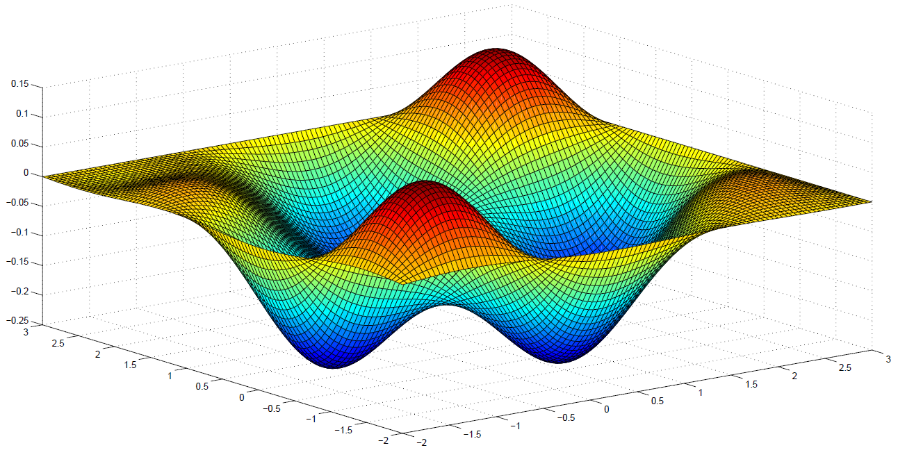
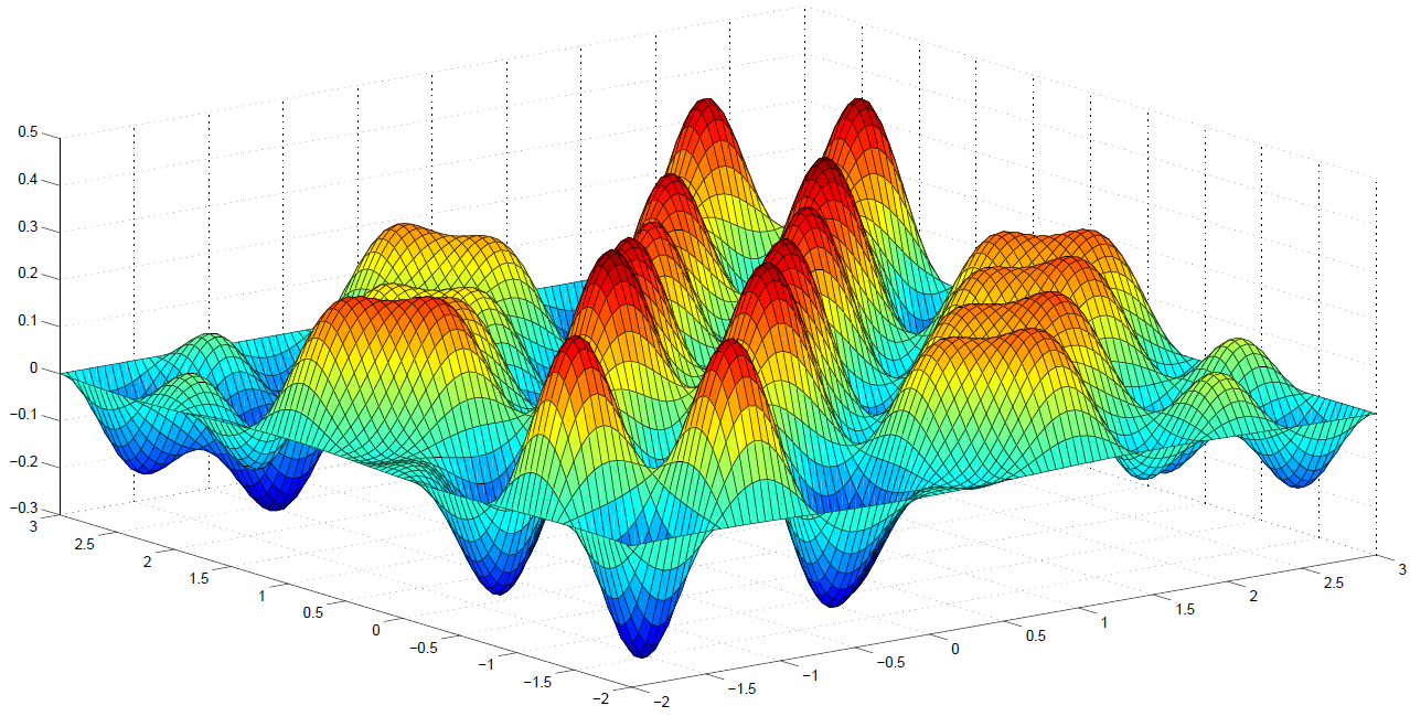
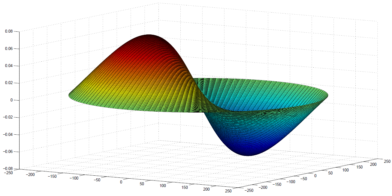
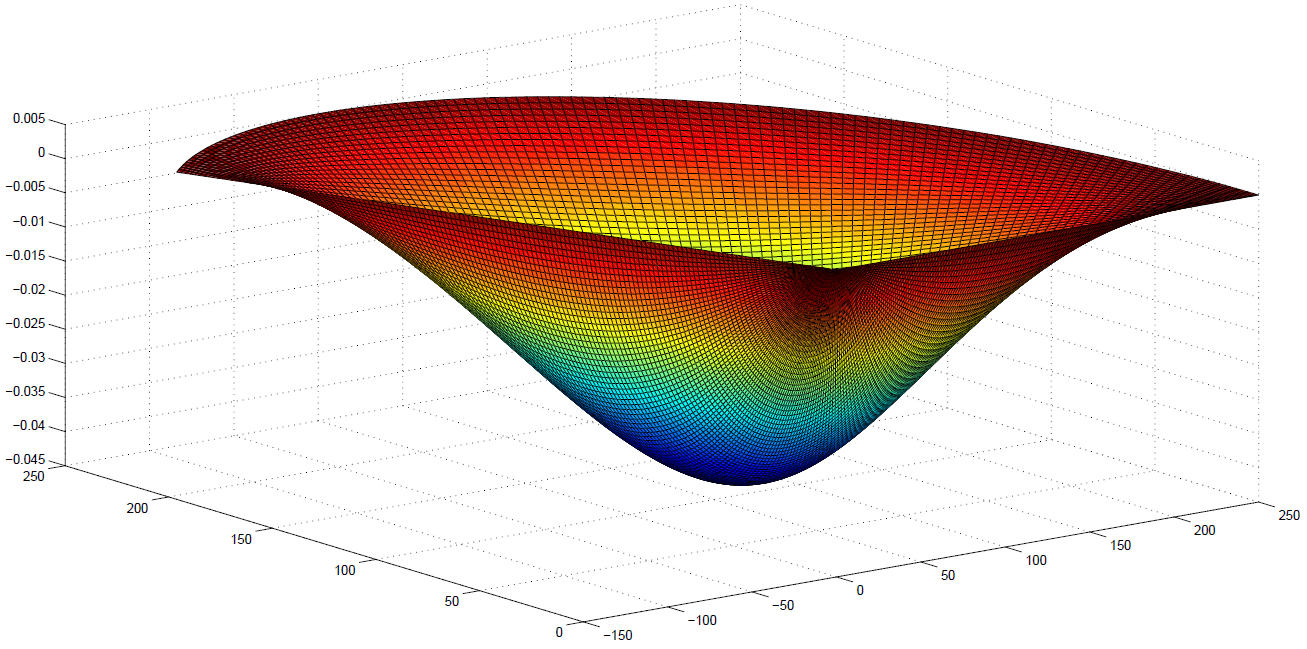
In Table 1, hxsubscript𝑥h_{x} and hysubscript𝑦h_{y} refer to the discretization step size at each dimension. In the cases (P1,a,C1) and (P2,a,C2), a generation of a functional value (surface) of the response is respectively represented in Figures 12.

Refer to caption
Figure 1: Case (P1,a,C1). Simulated response with p=4𝑝4p=4, TR=16𝑇𝑅16TR=16 and 𝜷𝜷\boldsymbol{\beta} of type C1.
Refer to caption
Figure 2: Case (P2,a,C2). Simulated response with p=9𝑝9p=9, TR=16𝑇𝑅16TR=16 and 𝜷𝜷\boldsymbol{\beta} of type C2.

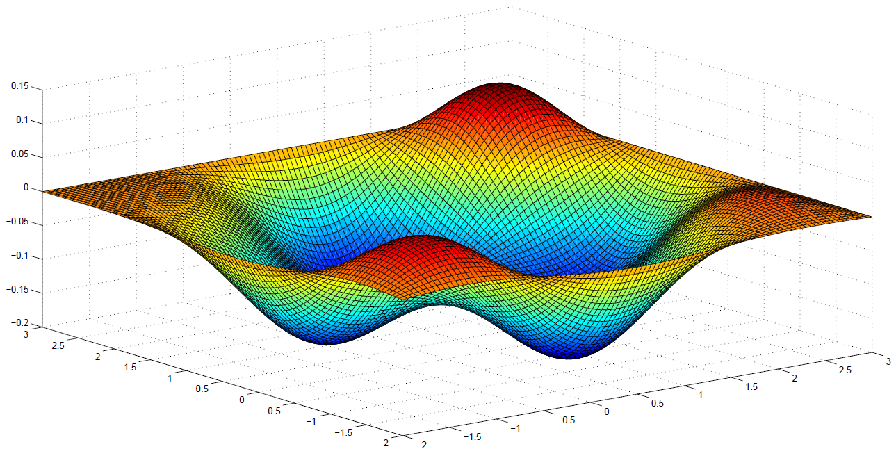
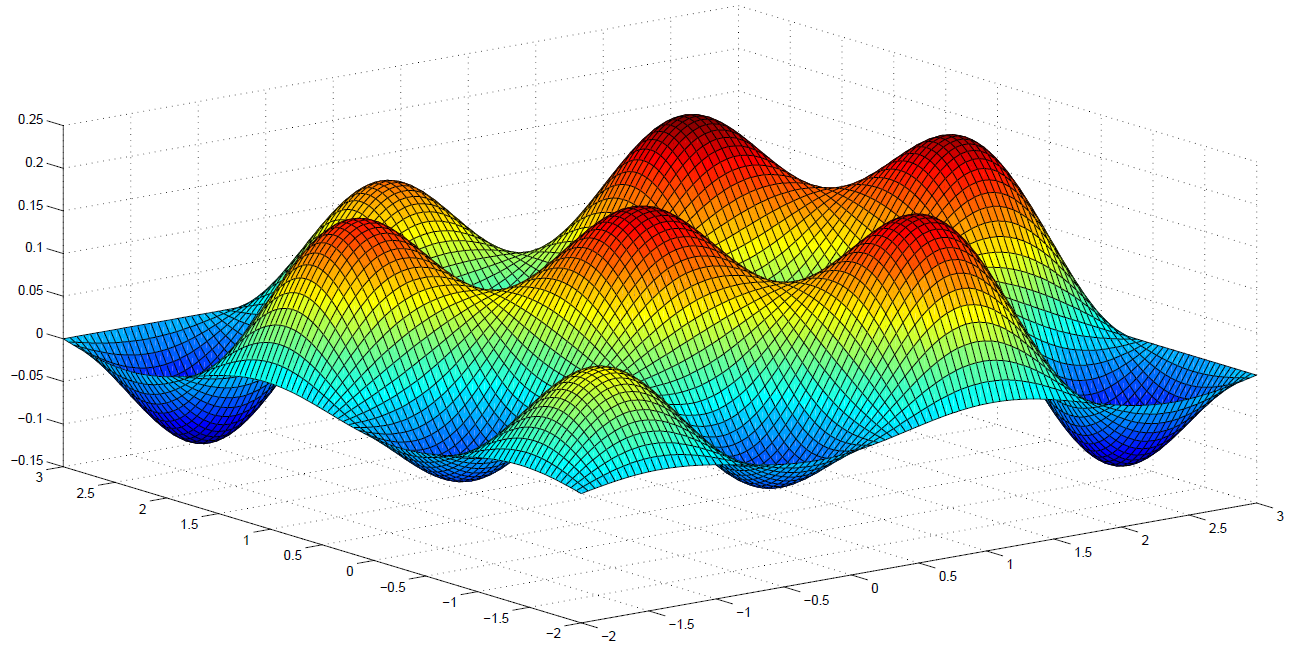
Figures 34 below show the respective functional estimates 𝐘^=𝐗𝜷^^𝐘𝐗^𝜷\widehat{\mathbf{Y}}=\mathbf{X}\widehat{\boldsymbol{\beta}} of the responses displayed in Figures 12 above.


Refer to caption
Figure 3: Case (P1,a,C1). Estimated response with p=4𝑝4p=4, TR=16𝑇𝑅16TR=16 and 𝜷𝜷\boldsymbol{\beta} of type C1.
Refer to caption
Figure 4: Case (P2,a,C2). Estimated response with p=9𝑝9p=9, TR=16𝑇𝑅16TR=16 and 𝜷𝜷\boldsymbol{\beta} of type C2.

The statistics (33)–(34) are evaluated in all the cases displayed in Table 1 (see Tables 23 for the statistics L𝜷superscriptsubscript𝐿𝜷L_{\boldsymbol{\beta}}^{\infty} and L𝐘,superscriptsubscript𝐿𝐘L_{\mathbf{Y}}^{\infty}, respectively).


Table 2: EFMSE𝜷𝐸𝐹𝑀𝑆subscript𝐸𝜷EFMSE_{\boldsymbol{\beta}} for rectangular domain.

EFMSE𝜷𝐸𝐹𝑀𝑆subscript𝐸𝜷EFMSE_{\boldsymbol{\beta}}
(P1,a,C1) (P1,b,C2) (P1,c,C2) (P1,d,C2) 1.070(10)31.070superscript1031.070\left(10\right)^{-3} 1.060(10)31.060superscript1031.060\left(10\right)^{-3} 1.040(10)31.040superscript1031.040\left(10\right)^{-3} 1.040(10)31.040superscript1031.040\left(10\right)^{-3} (P2,a,C2) (P2,b,C1) (P2,c,C1) (P2,d,C2) 9.400(10)49.400superscript1049.400\left(10\right)^{-4} 9.300(10)49.300superscript1049.300\left(10\right)^{-4} 9.300(10)49.300superscript1049.300\left(10\right)^{-4} 9.100(10)49.100superscript1049.100\left(10\right)^{-4}


Table 3: EFMSE𝐘𝐸𝐹𝑀𝑆subscript𝐸𝐘EFMSE_{\mathbf{Y}} for rectangular domain.

EFMSE𝐘𝐸𝐹𝑀𝑆subscript𝐸𝐘EFMSE_{\mathbf{Y}}
(P1,a,C1) (P1,b,C2) (P1,c,C2) (P1,d,C2) (P2,a,C2) (P2,b,C1) (P2,c,C1) (P2,d,C2) 0.0140.0140.014 0.0130.0130.013 0.0100.0100.010 0.0090.0090.009 0.0110.0110.011 0.0110.0110.011 0.0090.0090.009 0.0070.0070.007


As expected, the results displayed in Table 2, corresponding to the empirical functional mean quadratic errors associated with the estimation of 𝜷,𝜷\boldsymbol{\beta}, are less than the ones obtained in Table 3 for the response, with order of magnitude 103superscript10310^{-3} in all the scenarios generated. In Table 3, we can appreciate a better performance of the generalized least–squares estimator for the higher truncation orders. However, we have to note that, even for the smallest truncation order considered; i.e., for TR=4×4=16,𝑇𝑅4416TR=4\times 4=16, a good performance is observed with associated empirical functional mean quadratic errors having order of magnitude 102superscript10210^{-2} in all the cases displayed in Table 1 (see the above truncation order criteria (i)–(iii)). It can also be observed that the number of components of parameter 𝜷,𝜷\boldsymbol{\beta}, and their functional shapes do not affect the accuracy of the least–squares generalized estimations of the functional values of the response. It can also be observed that the number of components of parameter 𝜷,𝜷\boldsymbol{\beta}, and their functional shapes do not affect the accuracy of the least–squares generalized estimations of the functional values of the response.


The statistics (25) is now computed, as an empirical approximation of the relative magnitude between the explained functional variability and the residual variability, after fitting the transformed Hilbert–valued fixed effect model (23). The results obtained are given in Table 4. It can be observed that, in all the cases studied, the explained functional variability exceeds the residual functional variability. The truncation order, the number of components of 𝜷,𝜷\boldsymbol{\beta}, and the functional shape of such components do not substantially affect the goodness of fit of the transformed Hilbert–valued fixed effect model in (23).


Table 4: F𝐹F statistics (25) for rectangular domain.
Cases (P1,a,C1) (P1,b,C2) (P1,c,C2) (P1,d,C1) (P2,a,C2subscript𝐶2C_{2}) (P2subscript𝑃2P_{2},b,C1subscript𝐶1C_{1}) (P2,c,C1) (P2,d,C2)
F𝐹F 1.9261.9261.926 1.7171.7171.717 1.6731.6731.673 1.6261.6261.626 1.8981.8981.898 1.8451.8451.845 1.7611.7611.761 1.6061.6061.606

Let us now compute the statistics T𝒉subscript𝑇𝒉T_{\boldsymbol{h}} in (30) to contrast the significance of parameter vector 𝜷𝜷\boldsymbol{\beta} in Case C1,1{}_{1}, when p=4.𝑝4p=4. To apply [Cuesta-Albertos et al., 2007, Theorem 4.1] and [Cuesta-Albertos and Febrero-Bande, 2010, Theorem 2.1], we have generated eight realizations of a Gaussian random function 𝒉,𝒉\boldsymbol{h}, from the trajectories of the Gaussian random field ξ,𝜉\xi, solution, in the mean–square sense, of the following boundary value problem:

(Δ)ξ(𝐱)Δ𝜉𝐱\displaystyle(-\Delta)\xi(\mathbf{x}) =\displaystyle= ς(𝐱),𝐱=(x1,x2)[2,3]×[2,3],𝜍𝐱𝐱subscript𝑥1subscript𝑥22323\displaystyle\varsigma(\mathbf{x}),\quad\mathbf{x}=(x_{1},x_{2})\in[-2,3]\times[-2,3],
ξ(2,x2)𝜉2subscript𝑥2\displaystyle\xi(-2,x_{2}) =\displaystyle= ξ(3,x2)=ξ(x1,2)=ξ(x1,3)=0,x1,x2[2,3]×[2,3],formulae-sequence𝜉3subscript𝑥2𝜉subscript𝑥12𝜉subscript𝑥130subscript𝑥1subscript𝑥22323\displaystyle\xi(3,x_{2})=\xi(x_{1},-2)=\xi(x_{1},3)=0,\quad x_{1},x_{2}\in[-2,3]\times[-2,3],

where ς𝜍\varsigma denotes a zero–mean Gaussian white noise on L2([2,3]×[2,3])superscript𝐿22323L^{2}([-2,3]\times[-2,3]); i.e., a zero–mean generalized Gaussian process satisfying

[2,3]×[2,3]f(𝐱)E{ς(𝐲)ς(𝐱)}𝑑𝐱=f(𝐲),𝐲[2,3]×[2,3],fL2([2,3]×[2,3]).formulae-sequencesubscript2323𝑓𝐱E𝜍𝐲𝜍𝐱differential-d𝐱𝑓𝐲formulae-sequence𝐲2323for-all𝑓superscript𝐿22323\displaystyle\displaystyle\int_{[-2,3]\times[-2,3]}f(\mathbf{x}){\rm E}\left\{\varsigma(\mathbf{y})\varsigma(\mathbf{x})\right\}d\mathbf{x}=f(\mathbf{y}),\quad\mathbf{y}\in[-2,3]\times[-2,3],\quad\forall f\in L^{2}([-2,3]\times[-2,3]).

Table 5 below reflects the percentage of successes, for α=0.05,𝛼0.05\alpha=0.05, and the averaged p𝑝p–values over the 150150150 samples of the response generated with parameter 𝜷𝜷\boldsymbol{\beta} of C1 type having p=4𝑝4p=4 components, and with size n=150,𝑛150n=150, for TR=4×4.𝑇𝑅44TR=4\times 4.


Table 5: Rectangle. Percentage of successes for α=0.05,𝛼0.05\alpha=0.05, at the left–hand side, and averaged p𝑝p–values at the right–hand side, for each one of the eight realizations considered of the Gaussian function hL2([2,3]×[2,3]).superscript𝐿22323h\in L^{2}([-2,3]\times[-2,3]).
D𝐷D %percent\% Success p𝑝p
1 100%percent100100\% 00
2 100%percent100100\% 00
3 99.75%percent99.7599.75\% 1.998(10)81.998superscript1081.998(10)^{-8}
4 100%percent100100\% 00
5 99.8%percent99.899.8\% 7.541(10)77.541superscript1077.541(10)^{-7}
6 100%percent100100\% 00
7 100%percent100100\% 00
8 100%percent100100\% 6.441(10)106.441superscript10106.441(10)^{-10}

A high percentage of successes and very small p𝑝p–values are observed in Table 5; i.e., a good performance of the test statistics is observed.

Disk domain

In the disk domain

D2={𝐱2: 0<𝐱<R},subscript𝐷2conditional-set𝐱superscript2 0norm𝐱𝑅D_{2}=\left\{\mathbf{x}\in\mathbb{R}^{2}:\leavevmode\nobreak\ 0<\|\mathbf{x}\|<R\right\},

the zero–mean Gaussian Hnsuperscript𝐻𝑛H^{n}–valued error term is generated from the matrix covariance operator 𝑹𝜺𝜺,subscript𝑹𝜺𝜺\boldsymbol{R}_{\boldsymbol{\varepsilon}\boldsymbol{\varepsilon}}, whose functional entries are defined in equation (32), considering the eigenvectors {ϕk,k1}subscriptitalic-ϕ𝑘𝑘1\{\phi_{k},\ k\geq 1\} of the Dirichlet negative Laplacian operator on the disk (see equation (47) in the Supplementary Material in Appendix 7), arranged in decreasing order of the modulus magnitude of their associated eigenvalues. Specifically, for i=1,,n,𝑖1𝑛i=1,\dots,n, λki=λk(Rii)subscript𝜆𝑘𝑖subscript𝜆𝑘subscript𝑅𝑖𝑖\lambda_{ki}=\lambda_{k}(R_{ii}) in (32) is defined in equations (LABEL:A4:covopf) and (47). Again, ν=20𝜈20\nu=20 functional samples of size n=200𝑛200n=200 of the response have been generated. The cases studied are summarized in terms of the vector (Pi, u, Cj), i=1,2,𝑖12i=1,2, j=1,2,3,𝑗123j=1,2,3, with variable u=a,b,c,d,e,f.𝑢𝑎𝑏𝑐𝑑𝑒𝑓u=a,b,c,d,e,f. Namely, it is considered u=a𝑢𝑎u=a for TR=3,𝑇𝑅3TR=3, u=b𝑢𝑏u=b for TR=5,𝑇𝑅5TR=5, u=c𝑢𝑐u=c for TR=7,𝑇𝑅7TR=7, u=d𝑢𝑑u=d for TR=15,𝑇𝑅15TR=15, u=e𝑢𝑒u=e for TR=31,𝑇𝑅31TR=31, and u=f𝑢𝑓u=f for TR=79.𝑇𝑅79TR=79. Furthermore, Pi indicates the number of components of 𝜷,𝜷\boldsymbol{\beta}, with p=4𝑝4p=4 for i=1,𝑖1i=1, and p=9𝑝9p=9 for i=2.𝑖2i=2. Finally, the values of Cj,𝑗{}_{j}, j=1,2,3,𝑗123j=1,2,3, refer to the shape of the components of 𝜷,𝜷\boldsymbol{\beta}, defined from their projections, in terms of the following equations:

βkssubscript𝛽𝑘𝑠\displaystyle\beta_{ks} =\displaystyle= (1)sk3.5e(kTR)7.5+2s1P(s,k)2.5+2s1superscript1𝑠superscript𝑘3.5superscript𝑒superscript𝑘𝑇𝑅7.52𝑠1𝑃superscript𝑠𝑘2.52𝑠1\displaystyle\frac{\left(-1\right)^{s}}{k^{3.5}}e^{\left(\frac{k}{TR}\right)^{7.5+2s-1}}P\left(s,k\right)^{2.5+2s-1}
+\displaystyle+ e(kTR)6.5+2s1P(s,k)3.5+2s1,k=1,,TR,s=1,,p(C1)formulae-sequencesuperscript𝑒superscript𝑘𝑇𝑅6.52𝑠1𝑃superscript𝑠𝑘3.52𝑠1𝑘1𝑇𝑅𝑠1𝑝(C1)\displaystyle e^{\left(\frac{k}{TR}\right)^{6.5+2s-1}}P\left(s,k\right)^{3.5+2s-1},\quad k=1,\dots,TR,\quad s=1,\dots,p\quad\mbox{({\color[rgb]{0.6471,0.1098,0.1882}\definecolor[named]{pgfstrokecolor}{rgb}{0.6471,0.1098,0.1882}C1})}
βkssubscript𝛽𝑘𝑠\displaystyle\beta_{ks} =\displaystyle= 1Res+kRn+kcos((1)k2πRk),k=1,,TR,s=1,,p(C2)formulae-sequence1𝑅superscript𝑒𝑠𝑘𝑅𝑛𝑘superscript1𝑘2𝜋𝑅𝑘𝑘1𝑇𝑅𝑠1𝑝(C2)\displaystyle\frac{1}{R}e^{\frac{s+\frac{k}{R}}{n}}+k\cos\left(\left(-1\right)^{k}2\pi\frac{R}{k}\right),\quad k=1,\dots,TR,\quad s=1,\dots,p\quad\mbox{({\color[rgb]{0.6471,0.1098,0.1882}\definecolor[named]{pgfstrokecolor}{rgb}{0.6471,0.1098,0.1882}C2})}
βkssubscript𝛽𝑘𝑠\displaystyle\beta_{ks} =\displaystyle= 1k2.5+2s1P(s,k)1.5+2s1,k=1,,TR,s=1,,p(C3)formulae-sequence1superscript𝑘2.52𝑠1𝑃superscript𝑠𝑘1.52𝑠1𝑘1𝑇𝑅𝑠1𝑝(C3)\displaystyle\frac{1}{k^{2.5+2s-1}}P\left(s,k\right)^{1.5+2s-1},\quad k=1,\dots,TR,\quad s=1,\dots,p\quad\mbox{({\color[rgb]{0.6471,0.1098,0.1882}\definecolor[named]{pgfstrokecolor}{rgb}{0.6471,0.1098,0.1882}C3})}
P(s,k)𝑃𝑠𝑘\displaystyle P\left(s,k\right) =\displaystyle= 1+(kTR)2+(TRk+1TR)4,k=1,,TR,s=1,,p.formulae-sequence1superscript𝑘𝑇𝑅2superscript𝑇𝑅𝑘1𝑇𝑅4𝑘1𝑇𝑅𝑠1𝑝\displaystyle 1+\left(\frac{k}{TR}\right)^{2}+\left(\frac{TR-k+1}{TR}\right)^{4},\quad k=1,\dots,TR,\quad s=1,\dots,p.

Table 6 reflects a summary with all the cases analysed.


Table 6: Scenarios for disk domain.
Cases R𝑅R hRsubscript𝑅h_{R} hϕsubscriptitalic-ϕh_{\phi} TR𝑇𝑅TR p𝑝p
(P1,a,C3) 121212 R145𝑅145\frac{R}{145} 2π1352𝜋135\frac{2\pi}{135} 333 444
(P1,b,C2) 181818 R145𝑅145\frac{R}{145} 2π1352𝜋135\frac{2\pi}{135} 555 444
(P1,c,C1) 252525 R145𝑅145\frac{R}{145} 2π1352𝜋135\frac{2\pi}{135} 777 444
(P1,d,C1) 505050 R145𝑅145\frac{R}{145} 2π1352𝜋135\frac{2\pi}{135} 151515 444
(P1,e,C2) 100100100 R145𝑅145\frac{R}{145} 2π1352𝜋135\frac{2\pi}{135} 313131 444
(P1,f,C3) 250250250 R145𝑅145\frac{R}{145} 2π1352𝜋135\frac{2\pi}{135} 797979 444
(P2,a,C1) 121212 R145𝑅145\frac{R}{145} 2π1352𝜋135\frac{2\pi}{135} 333 999
(P2,b,C2) 181818 R145𝑅145\frac{R}{145} 2π1352𝜋135\frac{2\pi}{135} 555 999
(P2,c,C3) 252525 R145𝑅145\frac{R}{145} 2π1352𝜋135\frac{2\pi}{135} 777 999
(P2,d,C3) 505050 R145𝑅145\frac{R}{145} 2π1352𝜋135\frac{2\pi}{135} 151515 999
(P2,e,C2) 100100100 R145𝑅145\frac{R}{145} 2π1352𝜋135\frac{2\pi}{135} 313131 999
(P2,f,C1) 250250250 R145𝑅145\frac{R}{145} 2π1352𝜋135\frac{2\pi}{135} 797979 999

Figures 56 respectively reflect the generation of a functional value of the response in the cases (P1,c,C1) and (P1,f,C3).
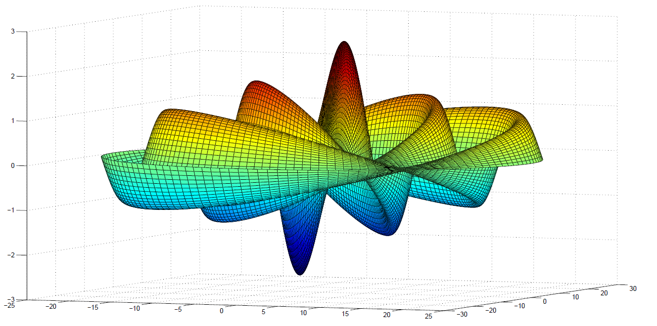
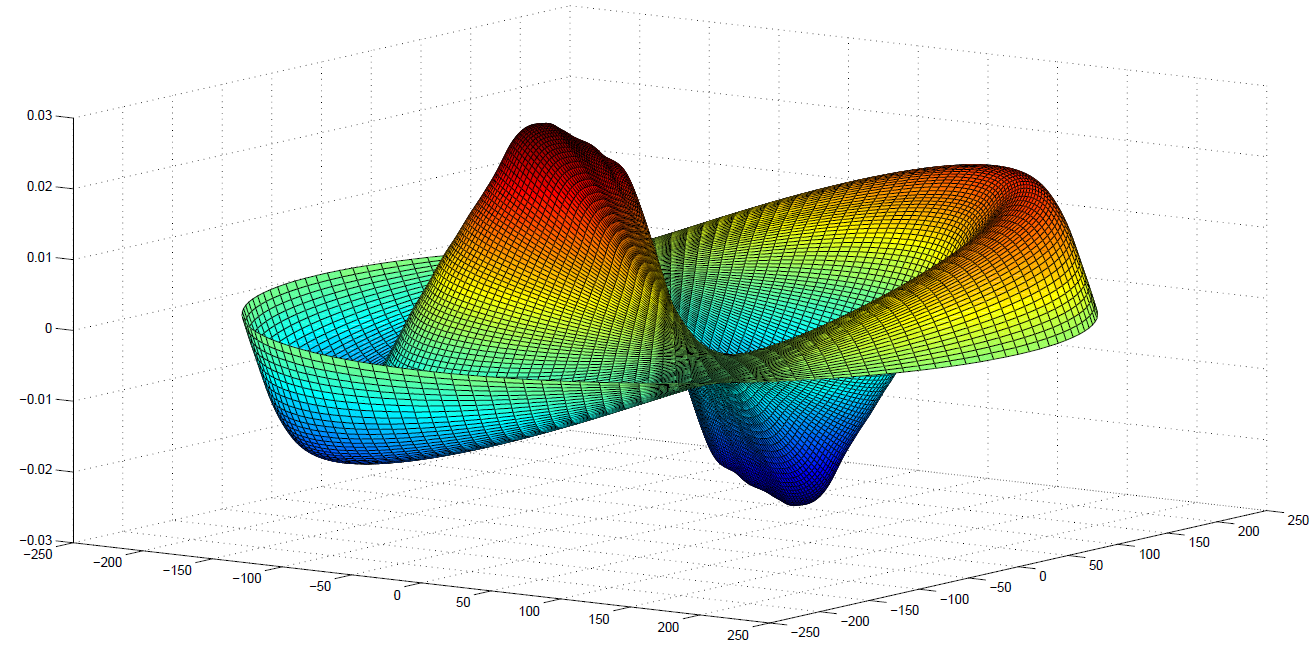
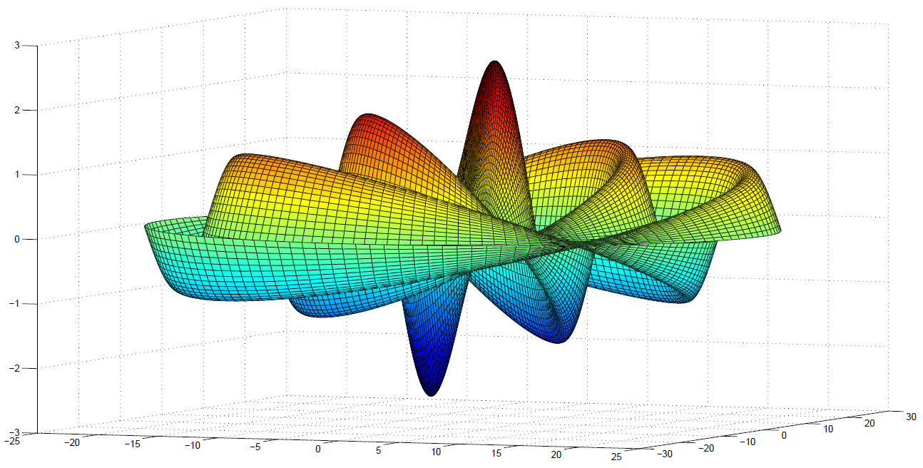
Refer to caption
Figure 5: Case (P1,c,C1). Simulated response with p=4𝑝4p=4, R=25𝑅25R=25 and 𝜷𝜷\boldsymbol{\beta} of type C1.
Refer to caption
Figure 6: Case (P1,f,C3). Simulated response with p=4𝑝4p=4, R=250𝑅250R=250 and 𝜷𝜷\boldsymbol{\beta} of type C3.

The respective generalized least–squares functional estimates are displayed in Figures 78.


Refer to caption
Figure 7: Case (P1,c,C1). Estimated response with p=4𝑝4p=4, R=25𝑅25R=25 and 𝜷𝜷\boldsymbol{\beta} of type C1subscript𝐶1C_{1}.
Refer to caption
Figure 8: Case (P1,f,C3). Estimated response with p=4𝑝4p=4, R=250𝑅250R=250 and 𝜷𝜷\boldsymbol{\beta} of type C3subscript𝐶3C_{3}.

The empirical functional mean quadratic errors (see equations (33)–(34)) are displayed in Table 7, for the estimation of the functional parameter vector 𝜷,𝜷\boldsymbol{\beta}, and in Table 8 for the estimation of the response 𝐘𝐘\mathbf{Y}. It can be observed, as in the rectangular domain, that the order of magnitude of the empirical functional mean quadratic errors associated with the estimation of 𝜷𝜷\boldsymbol{\beta} is of order 103,superscript10310^{-3}, and for the estimation of the response is 102superscript10210^{-2}. However, the number of terms considered is less than in the case of the rectangle; i.e., a finite dimensional space with lower dimension than in the rectangle is required, according to criterion (iii) reflected in Appendix 4. It can also be appreciated that the number of components of 𝜷𝜷\boldsymbol{\beta} does not substantially affect the accuracy of the estimates.


Table 7: EFMSE𝜷𝐸𝐹𝑀𝑆subscript𝐸𝜷EFMSE_{\boldsymbol{\beta}} for disk domain.

EFMSE𝜷𝐸𝐹𝑀𝑆subscript𝐸𝜷EFMSE_{\boldsymbol{\beta}}
(P1,a,C3) (P1,b,C2) (P1,c,C1) 7.500(10)47.500superscript1047.500\left(10\right)^{-4} 7.500(10)47.500superscript1047.500\left(10\right)^{-4} 7.400(10)47.400superscript1047.400\left(10\right)^{-4} (P1,d,C1) (P1,e,C2) (P1,f,C3) 7.500(10)47.500superscript1047.500\left(10\right)^{-4} 7.600(10)47.600superscript1047.600\left(10\right)^{-4} 7.500(10)47.500superscript1047.500\left(10\right)^{-4} (P2,a,C1) (P2,b,C2) (P2,c,C3) 7.000(10)47.000superscript1047.000\left(10\right)^{-4} 7.100(10)47.100superscript1047.100\left(10\right)^{-4} 7.100(10)47.100superscript1047.100\left(10\right)^{-4} (P2,d,C3) (P2,e,C2) (P2,f,C1) 7.900(10)47.900superscript1047.900\left(10\right)^{-4} 8.000(10)48.000superscript1048.000\left(10\right)^{-4} 8.000(10)48.000superscript1048.000\left(10\right)^{-4}


Table 8: EFMSE𝐘𝐸𝐹𝑀𝑆subscript𝐸𝐘EFMSE_{\mathbf{Y}} for disk domain.

EFMSE𝐘𝐸𝐹𝑀𝑆subscript𝐸𝐘EFMSE_{\mathbf{Y}}
(P1,a,C3) (P1,b,C2) (P1,c,C1) (P1,d,C1) (P1,e,C2) (P1,f,C3) 0.0480.0480.048 0.0480.0480.048 0.0480.0480.048 0.0480.0480.048 0.0480.0480.048 0.0480.0480.048 (P2,a,C1) (P2,b,C2) (P2,c,C3) (P2,d,C3) (P2,e,C2) (P2,f,C1) 0.0500.0500.050 0.0500.0500.050 0.0500.0500.050 0.0490.0490.049 0.0500.0500.050 0.0500.0500.050


The statistics (25) is now computed (see Table 9), as an empirical approximation of the relative magnitude between the explained functional variability and the residual variability, after fitting the transformed Hilbert-valued fixed effect model (23). It can be noticed that the values of SSR~SST~~𝑆𝑆𝑅~𝑆𝑆𝑇\frac{\widetilde{SSR}}{\widetilde{SST}} are very close to one in all the scenarios analysed. This fact induces large values of (25) (see Table 9), since

F=SSR~SSE~=SSR~/SST~1SSR~/SST~.𝐹~𝑆𝑆𝑅~𝑆𝑆𝐸~𝑆𝑆𝑅~𝑆𝑆𝑇1~𝑆𝑆𝑅~𝑆𝑆𝑇F=\frac{\widetilde{SSR}}{\widetilde{SSE}}=\frac{\widetilde{SSR}/\widetilde{SST}}{1-\widetilde{SSR}/\widetilde{SST}}.

It can be observed, one time more, from criterion (iii), reflected in Appendix 4, that the boundary conditions and the geometry of the domain allows in this case a more substantial dimension reduction than in the rectangular domain case, since with lower truncation orders a better model fitting is obtained.


Table 9: F𝐹F statistics (25) over the disk domain.
Cases (P1,a,C3) (P1,b,C2) (P1,c,C1)
F𝐹F 1.100(102)1.100superscript1021.100(10^{2}) 4.100(103)4.100superscript1034.100(10^{3}) 1.200(105)1.200superscript1051.200(10^{5})
Cases (P1,d,C1) (P1,e,C2) (P1,f,C3)
F𝐹F 3.900(106)3.900superscript1063.900(10^{6}) 6.300(106)6.300superscript1066.300(10^{6}) 4.200(106)4.200superscript1064.200(10^{6})
Cases (P2,a,C1) (P2,b,C2) (P2,c,C3)
F𝐹F 2.200(103)2.200superscript1032.200(10^{3}) 8.200(103)8.200superscript1038.200(10^{3}) 7.600(107)7.600superscript1077.600(10^{7})
Cases (P2,d,C3) (P2,e,C2) (P2,f,C1)
F𝐹F 2.500(107)2.500superscript1072.500(10^{7}) 1.400(107)1.400superscript1071.400(10^{7}) 8.500(107)8.500superscript1078.500(10^{7})

The statistics T𝒉subscript𝑇𝒉T_{\boldsymbol{h}} in (30) is computed to contrast the significance of the parameter vector 𝜷𝜷\boldsymbol{\beta} in case C1,1{}_{1}, with p=4𝑝4p=4 components. Again, eight realizations of Gaussian random functions 𝒉𝒉\boldsymbol{h} are considered, generated from a Gaussian random field ξ,𝜉\xi, solution, in the mean–square sense, of the following boundary value problem on the disk:

(Δ)ξ(𝐱)Δ𝜉𝐱\displaystyle(-\Delta)\xi(\mathbf{x}) =\displaystyle= ς(𝐱),𝐱=(x1,x2)D25={𝐱2; 0<𝐱<25},𝜍𝐱𝐱subscript𝑥1subscript𝑥2subscript𝐷25formulae-sequence𝐱superscript2 0norm𝐱25\displaystyle\varsigma(\mathbf{x}),\quad\mathbf{x}=(x_{1},x_{2})\in D_{25}=\{\mathbf{x}\in\mathbb{R}^{2};\ 0<\|\mathbf{x}\|<25\},
ξ(θ,25)𝜉𝜃25\displaystyle\xi(\theta,25) =\displaystyle= 0,θ[0,2π]0for-all𝜃02𝜋\displaystyle 0,\quad\forall\theta\in[0,2\pi]

where ς𝜍\varsigma denotes a zero–mean Gaussian white noise on L2(D25)superscript𝐿2subscript𝐷25L^{2}(D_{25}); i.e., a zero–mean generalized Gaussian process satisfying

[0,2π]×[0,25]f(φ,v)E{ς(θ,r)ς(φ,v)}𝑑φ𝑑v=f(θ,r),(θ,r)[0,2π]×[0,25],fL2(D25).formulae-sequencesubscript02𝜋025𝑓𝜑𝑣E𝜍𝜃𝑟𝜍𝜑𝑣differential-d𝜑differential-d𝑣𝑓𝜃𝑟formulae-sequence𝜃𝑟02𝜋025𝑓superscript𝐿2subscript𝐷25\displaystyle\displaystyle\int_{[0,2\pi]\times[0,25]}f(\varphi,v){\rm E}\left\{\varsigma(\theta,r)\varsigma(\varphi,v)\right\}d\varphi dv=f(\theta,r),\quad(\theta,r)\in[0,2\pi]\times[0,25],\quad f\in L^{2}(D_{25}).

Table 10 reflects the percentage of successes, for α=0.05,𝛼0.05\alpha=0.05, and the averaged p𝑝p–values over the 150150150 samples, generated with size n=150,𝑛150n=150, of the functional response having parameter vector 𝜷𝜷\boldsymbol{\beta} of type C1 with p=4𝑝4p=4 components, for TR=7.𝑇𝑅7TR=7.


Table 10: Disk. Percentage of successes for α=0.05,𝛼0.05\alpha=0.05, at the left–hand side, and averaged p𝑝p–values at the right–hand side, for each one of the eight realizations of the Gaussian function hL2(D25).superscript𝐿2subscript𝐷25h\in L^{2}(D_{25}).
D𝐷D % Success p𝑝p
1 99.95%percent99.9599.95\% 1.672(10)81.672superscript1081.672(10)^{-8}
2 99.5%percent99.599.5\% 9.746(10)79.746superscript1079.746(10)^{-7}
3 100%percent100100\% 00
4 99.9%percent99.999.9\% 8.546(10)88.546superscript1088.546(10)^{-8}
5 97.45%percent97.4597.45\% 7.400(10)77.400superscript1077.400(10)^{-7}
6 100%percent100100\% 00
7 100%percent100100\% 8.775(10)98.775superscript1098.775(10)^{-9}
8 100%percent100100\% 00

Table 10 again illustrates a good performance of the statistics T𝒉subscript𝑇𝒉T_{\boldsymbol{h}} in (30). Indeed, we can appreciate a high percentage of successes, and very small p𝑝p–values, very close to zero, that support the significance of the functional parameter vector, considered in the generation of the data set analysed.

Circular sector domain

In the circular sector

D3={(rcos(φ),rsin(φ)): 0<r<R, 0<φ<πθ}subscript𝐷3conditional-set𝑟𝜑𝑟𝜑formulae-sequence 0norm𝑟𝑅 0𝜑𝜋𝜃D_{3}=\left\{\left(r\cos\left(\varphi\right),\leavevmode\nobreak\ r\sin\left(\varphi\right)\right):\leavevmode\nobreak\ 0<\|r\|<R,\leavevmode\nobreak\ 0<\varphi<\pi\theta\right\}

of radius R𝑅R and angle πθ,𝜋𝜃\pi\theta, the zero-mean Gaussian vector error term is generated from the matrix covariance operator 𝑹𝜺𝜺,subscript𝑹𝜺𝜺\boldsymbol{R}_{\boldsymbol{\varepsilon}\boldsymbol{\varepsilon}}, whose functional entries are defined in equation (32). The eigenvectors {ϕk,k1}subscriptitalic-ϕ𝑘𝑘1\{\phi_{k},\ k\geq 1\} of the Dirichlet negative Laplacian operator on the circular sector are considered (see equation (LABEL:A4:eqcsa) in the Supplementary Material in Appendix 7), arranged in decreasing order of the modulus magnitude of their associated eigenvalues. Specifically, here, 𝑹𝜺𝜺subscript𝑹𝜺𝜺\boldsymbol{R}_{\boldsymbol{\varepsilon}\boldsymbol{\varepsilon}} is defined in equation (32), with for i=1,,n,𝑖1𝑛i=1,\dots,n, λki=λk(Rii)subscript𝜆𝑘𝑖subscript𝜆𝑘subscript𝑅𝑖𝑖\lambda_{ki}=\lambda_{k}(R_{ii}) being given in equations (LABEL:A4:covopf) and (LABEL:A4:eqcsa).

As in the above examples, ν=20𝜈20\nu=20 functional samples of size n=200𝑛200n=200 are generated. The cases studied are also summarized in terms of the values of the vector (Pi,u,Cj)subscript𝑃𝑖𝑢subscript𝐶𝑗(P_{i},u,C_{j}), i=1,2,u=a,b,c,d,e,f,formulae-sequence𝑖12𝑢𝑎𝑏𝑐𝑑𝑒𝑓i=1,2,\leavevmode\nobreak\ u=a,b,c,d,e,f, and j=1,2,3,𝑗123j=1,2,3, with the values of u𝑢u having the same meaning as in the disk domain. Again, values of Pisubscript𝑃𝑖P_{i} provide the number p𝑝p of components of 𝜷;𝜷\boldsymbol{\beta}; i.e., p=4𝑝4p=4 if i=1𝑖1i=1, and p=9𝑝9p=9 if i=2𝑖2i=2. The values C1,subscript𝐶1C_{1}, C2subscript𝐶2C_{2} and C3subscript𝐶3C_{3} respectively correspond to the following functions defining the components of 𝜷,𝜷\boldsymbol{\beta}, whose projections are given by:

βsksubscript𝛽𝑠𝑘\displaystyle\beta_{sk} =\displaystyle= 1+(k1)s,k=1,,TR,s=1,,p(C1)formulae-sequence1𝑘1𝑠𝑘1𝑇𝑅𝑠1𝑝(C1)\displaystyle 1+(k-1)s,\quad k=1,\dots,TR,\quad s=1,\dots,p\quad\mbox{({\color[rgb]{0.6471,0.1098,0.1882}\definecolor[named]{pgfstrokecolor}{rgb}{0.6471,0.1098,0.1882}C1})}
βsksubscript𝛽𝑠𝑘\displaystyle\beta_{sk} =\displaystyle= 1Res+kRn+kcos((1)k2πRk),k=1,,TR,s=1,,p(C2)formulae-sequence1𝑅superscript𝑒𝑠𝑘𝑅𝑛𝑘superscript1𝑘2𝜋𝑅𝑘𝑘1𝑇𝑅𝑠1𝑝(C2)\displaystyle\frac{1}{R}e^{\frac{s+\frac{k}{R}}{n}}+k\cos\left(\left(-1\right)^{k}2\pi\frac{R}{k}\right),\quad k=1,\dots,TR,\quad s=1,\dots,p\quad\mbox{({\color[rgb]{0.6471,0.1098,0.1882}\definecolor[named]{pgfstrokecolor}{rgb}{0.6471,0.1098,0.1882}C2})}
βsksubscript𝛽𝑠𝑘\displaystyle\beta_{sk} =\displaystyle= cos(πTRkk)cos(πpss),k=1,,TR,s=1,,p(C3).formulae-sequence𝜋𝑇𝑅𝑘𝑘𝜋𝑝𝑠𝑠𝑘1𝑇𝑅𝑠1𝑝(C3)\displaystyle\cos\left(\pi\frac{TR-k}{k}\right)\cos\left(\pi\frac{p-s}{s}\right),\quad k=1,\dots,TR,\quad s=1,\dots,p\quad\mbox{({\color[rgb]{0.6471,0.1098,0.1882}\definecolor[named]{pgfstrokecolor}{rgb}{0.6471,0.1098,0.1882}C3})}.

A summary of the cases analysed is given in Table 11.


Table 11: Scenarios for circular sector domain.
Cases R𝑅R hRsubscript𝑅h_{R} hϕsubscriptitalic-ϕh_{\phi} TR𝑇𝑅TR θ𝜃\theta p𝑝p
(P1,a,C3) 121212 R145𝑅145\frac{R}{145} 2π1152𝜋115\frac{2\pi}{115} 333 2323\frac{2}{3} 444
(P1,b,C2) 181818 R145𝑅145\frac{R}{145} 2π1152𝜋115\frac{2\pi}{115} 555 2323\frac{2}{3} 444
(P1,c,C1) 252525 R145𝑅145\frac{R}{145} 2π1152𝜋115\frac{2\pi}{115} 777 2323\frac{2}{3} 444
(P1,d,C1) 505050 R145𝑅145\frac{R}{145} 2π1152𝜋115\frac{2\pi}{115} 151515 2323\frac{2}{3} 444
(P1,e,C2) 100100100 R145𝑅145\frac{R}{145} 2π1152𝜋115\frac{2\pi}{115} 313131 2323\frac{2}{3} 444
(P1,f,C3) 250250250 R145𝑅145\frac{R}{145} 2π1152𝜋115\frac{2\pi}{115} 797979 2323\frac{2}{3} 444
(P2,a,C1) 121212 R145𝑅145\frac{R}{145} 2π1152𝜋115\frac{2\pi}{115} 333 2323\frac{2}{3} 999
(P2,b,C2) 181818 R145𝑅145\frac{R}{145} 2π1152𝜋115\frac{2\pi}{115} 555 2323\frac{2}{3} 999
(P2,c,C3) 252525 R145𝑅145\frac{R}{145} 2π1152𝜋115\frac{2\pi}{115} 777 2323\frac{2}{3} 999
(P2,d,C3) 505050 R145𝑅145\frac{R}{145} 2π1152𝜋115\frac{2\pi}{115} 151515 2323\frac{2}{3} 999
(P2,e,C2) 100100100 R145𝑅145\frac{R}{145} 2π1152𝜋115\frac{2\pi}{115} 313131 2323\frac{2}{3} 999
(P2,f,C1) 250250250 R145𝑅145\frac{R}{145} 2π1152𝜋115\frac{2\pi}{115} 797979 2323\frac{2}{3} 999

Figures 910 display the generation of a functional value of the response in the cases (P2,e,C2) and (P1,f,C3), respectively.
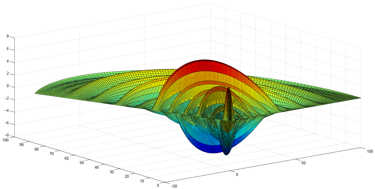
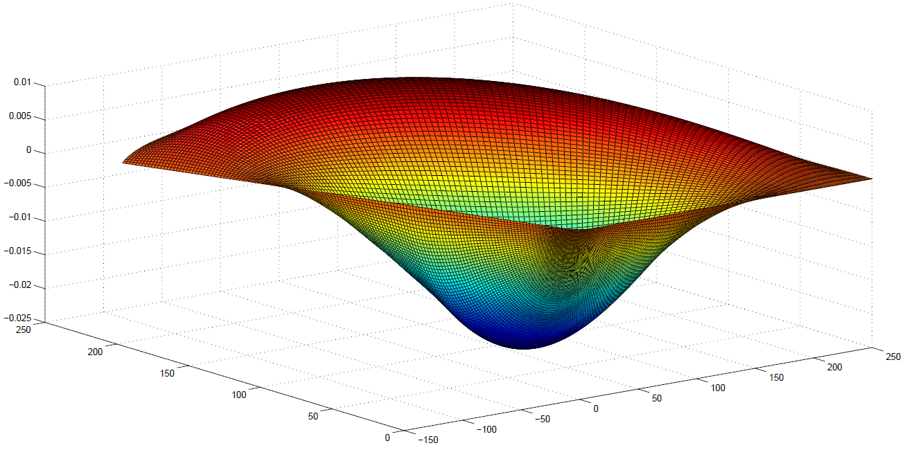
Refer to caption
Figure 9: Case (P2,e,C2). Simulated response with p=9𝑝9p=9, R=100𝑅100R=100 and 𝜷𝜷\boldsymbol{\beta} of type C2.
Refer to caption
Figure 10: Case (P1,f,C3). Simulated response with p=4𝑝4p=4, R=250𝑅250R=250 and 𝜷𝜷\boldsymbol{\beta} of type C3.

The functional estimates obtained from the finite–dimensional approximation of the generalized least–squares estimator of 𝜷𝜷\boldsymbol{\beta} are now given in Figures 1112, for the cases (P2,e,C2) and (P1,f,C3), respectively.
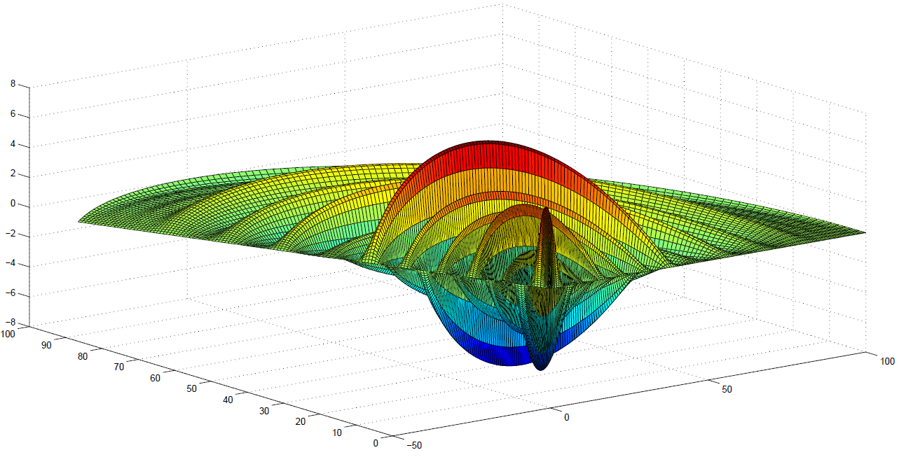

Refer to caption
Figure 11: Case (P2,e,C2). Estimated response with p=9𝑝9p=9, R=100𝑅100R=100 and 𝜷𝜷\boldsymbol{\beta} of type C2.
Refer to caption
Figure 12: Case (P1,f,C3). Estimated response with p=4𝑝4p=4, R=250𝑅250R=250 and 𝜷𝜷\boldsymbol{\beta} of type C3.

As in the previous sections, the empirical functional mean quadratic errors, associated with the estimation of 𝜷𝜷\boldsymbol{\beta} and 𝐘,𝐘\mathbf{Y}, are computed from equations (33)–(34). They are shown in Table 12, for 𝜷,𝜷\boldsymbol{\beta}, and in Table 13, for 𝐘.𝐘\mathbf{Y}.

These empirical functional mean quadratic errors are very stable through the different cases considered, and their order of magnitude is again 103superscript10310^{-3} for the parameter 𝜷,𝜷\boldsymbol{\beta}, and 102superscript10210^{-2} for the response. Here, the results displayed also correspond to the projection into lower finite–dimensional spaces than in the case of the rectangle, according to the functional form of the eigenvectors (see truncation order criterion (iii) in Appendix 4).


Table 12: EFMSE𝜷𝐸𝐹𝑀𝑆subscript𝐸𝜷EFMSE_{\boldsymbol{\beta}} for the circular sector.

EFMSE𝜷𝐸𝐹𝑀𝑆subscript𝐸𝜷EFMSE_{\boldsymbol{\beta}}
(P1,a,C3) (P1,b,C2) (P1,c,C1) 1.200(10)41.200superscript1041.200\left(10\right)^{-4} 1.100(10)41.100superscript1041.100\left(10\right)^{-4} 1.200(10)41.200superscript1041.200\left(10\right)^{-4} (P1,d,C1) (P1,e,C2) (P1,f,C3) 1.200(10)41.200superscript1041.200\left(10\right)^{-4} 1.200(10)41.200superscript1041.200\left(10\right)^{-4} 1.100(10)41.100superscript1041.100\left(10\right)^{-4} (P2,a,C1) (P2,b,C2) (P2,c,C3) 1.900(10)41.900superscript1041.900\left(10\right)^{-4} 2.000(10)42.000superscript1042.000\left(10\right)^{-4} 2.000(10)42.000superscript1042.000\left(10\right)^{-4} (P2,d,C3) (P2,e,C2) (P2,f,C1) 1.900(10)41.900superscript1041.900\left(10\right)^{-4} 1.900(10)41.900superscript1041.900\left(10\right)^{-4} 2.000(10)42.000superscript1042.000\left(10\right)^{-4}


Table 13: EFMSE𝐘𝐸𝐹𝑀𝑆subscript𝐸𝐘EFMSE_{\mathbf{Y}} for the circular sector.

EFMSE𝐘𝐸𝐹𝑀𝑆subscript𝐸𝐘EFMSE_{\mathbf{Y}}
(P1,a,C3) (P1,b,C2) (P1,c,C1) 8.770(10)38.770superscript1038.770\left(10\right)^{-3} 8.810(10)38.810superscript1038.810\left(10\right)^{-3} 8.820(10)38.820superscript1038.820\left(10\right)^{-3} (P1,d,C1) (P1,e,C2) (P1,f,C3) 8.820(10)38.820superscript1038.820\left(10\right)^{-3} 8.820(10)38.820superscript1038.820\left(10\right)^{-3} 8.810(10)38.810superscript1038.810\left(10\right)^{-3} (P2,a,C1) (P2,b,C2) (P2,c,C3) 9.630(10)39.630superscript1039.630\left(10\right)^{-3} 9.670(10)39.670superscript1039.670\left(10\right)^{-3} 9.670(10)39.670superscript1039.670\left(10\right)^{-3} (P2,d,C3) (P2,e,C2) (P2,f,C1) 9.670(10)39.670superscript1039.670\left(10\right)^{-3} 9.680(10)39.680superscript1039.680\left(10\right)^{-3} 9.660(10)39.660superscript1039.660\left(10\right)^{-3}


Statistics (25) is now computed. Its values are displayed in Table 14. Again, as in the disk, the proportion of explained functional variability is very close to one leading to large values of statistics (25), as it can be observed in Table 14 for all the cases analysed.


Table 14: F𝐹F statistics (25) for the circular sector.
Cases (P1,a,C3) (P1,b,C2) (P1,c,C1) (P1,d,C1) (P1,e,C2) (P1,f,C3)
F𝐹F 9.2(102)9.2superscript1029.2(10^{2}) 3.1(103)3.1superscript1033.1(10^{3}) 4.2(106)4.2superscript1064.2(10^{6}) 4.8(108)4.8superscript1084.8(10^{8}) 5.8(106))5.8(10^{6})) 7.3(108)7.3superscript1087.3(10^{8})
Cases (P2,a,C1) (P2,b,C2) (P2,c,C3) (P2,d,C3) (P2,e,C2) (P2,f,C1)
F𝐹F 1.8(103)1.8superscript1031.8(10^{3}) 4.1(103)4.1superscript1034.1(10^{3}) 2.6(107)2.6superscript1072.6(10^{7}) 3.1(109)3.1superscript1093.1(10^{9}) 6.8(106)6.8superscript1066.8(10^{6}) 1.8(109)1.8superscript1091.8(10^{9})

The statistics T𝒉subscript𝑇𝒉T_{\boldsymbol{h}} in (30) is computed to contrast the significance of the parameter vector 𝜷𝜷\boldsymbol{\beta} in case C1 with p=4𝑝4p=4 functional components. Eight realizations of a Gaussian random function 𝒉𝒉\boldsymbol{h} are considered from a Gaussian random field ξ,𝜉\xi, solution, in the mean-square sense, of the following boundary value problem on the circular sector

(Δ)ξ(𝐱)Δ𝜉𝐱\displaystyle(-\Delta)\xi(\mathbf{x}) =\displaystyle= ς(𝐱),𝐱=(rcos(φ),rsin(φ)), 0<r<R, 0<φ<πθ,formulae-sequence𝜍𝐱𝐱𝑟𝜑𝑟𝜑 0norm𝑟𝑅 0𝜑𝜋𝜃\displaystyle\varsigma(\mathbf{x}),\quad\mathbf{x}=\left(r\cos\left(\varphi\right),\leavevmode\nobreak\ r\sin\left(\varphi\right)\right),\leavevmode\nobreak\ 0<\|r\|<R,\leavevmode\nobreak\ 0<\varphi<\pi\theta,
ξ(φ,25)𝜉𝜑25\displaystyle\xi(\varphi,25) =\displaystyle= 0,φ[0,πθ],0𝜑0𝜋𝜃\displaystyle 0,\quad\varphi\in[0,\pi\theta],

where θ=2/3,𝜃23\theta=2/3, ς𝜍\varsigma denotes a zero–mean Gaussian white noise on the circular sector such that

[0,πθ]×[0,25]f(φ,v)E{ς(γ,r)ς(φ,v)}𝑑φ𝑑v=f(γ,r),(γ,r)[0,πθ]×[0,25],fL2(CS),formulae-sequencesubscript0𝜋𝜃025𝑓𝜑𝑣E𝜍𝛾𝑟𝜍𝜑𝑣differential-d𝜑differential-d𝑣𝑓𝛾𝑟formulae-sequence𝛾𝑟0𝜋𝜃025𝑓superscript𝐿2𝐶𝑆\displaystyle\displaystyle\int_{[0,\pi\theta]\times[0,25]}f(\varphi,v){\rm E}\left\{\varsigma(\gamma,r)\varsigma(\varphi,v)\right\}d\varphi dv=f(\gamma,r),\quad(\gamma,r)\in[0,\pi\theta]\times[0,25],\quad f\in L^{2}(CS),

with L2(CS)superscript𝐿2𝐶𝑆L^{2}(CS) denoting the space of square–integrable functions on the circular sector. Table 15 reflects the percentage of successes, for α=0.05,𝛼0.05\alpha=0.05, and the averaged p𝑝p–values over the 150150150 samples, with size n=150,𝑛150n=150, of the response, having C1–type functional parameter vector 𝜷𝜷\boldsymbol{\beta} with p=4𝑝4p=4 components, considering TR=7.𝑇𝑅7TR=7.


Table 15: Circular Sector. Percentage of successes for α=0.05,𝛼0.05\alpha=0.05, at the left–hand side, and averaged p𝑝p–values at the right–hand side, for each one of the eight realizations of the Gaussian function hL2(CS).superscript𝐿2𝐶𝑆h\in L^{2}(CS).
D𝐷D % Success p𝑝p
1 97.5%percent97.597.5\% 6.504(10)66.504superscript1066.504(10)^{-6}
2 100%percent100100\% 00
3 100%percent100100\% 3.600(10)83.600superscript1083.600(10)^{-8}
4 100%percent100100\% 00
5 98%percent9898\% 2.006(10)62.006superscript1062.006(10)^{-6}
6 99.5%percent99.599.5\% 9.807(10)89.807superscript1089.807(10)^{-8}
7 100%percent100100\% 00
8 99.5%percent99.599.5\% 4.111(10)74.111superscript1074.111(10)^{-7}

Table 15 again confirms the good performance of the test statistics T𝒉,subscript𝑇𝒉T_{\boldsymbol{h}}, showing a high percentage of successes, and very small magnitudes for the averaged p𝑝p–value (almost zero values), according to the significance of the parameter vector 𝜷𝜷\boldsymbol{\beta} considered in the generation of the analysed functional data set.

5 Functional statistical analysis of fMRI data

In this section, we compare the results obtained from the application of the MatLab function fmrilm.m (see Liao et al. [2012] and Worsley et al. [2002]) from fmristat.m function set (available at http://www.math.mcgill.ca/keith/fmristat), with those ones provided by the implementation of our proposed functional statistical methodology, based on the Hilbert-valued fixed effect models with ARH(1) error term above introduced. The fMRI data set analysed is also freely available in AFNI format at http://www.math.mcgill.ca/keith/fmristat/. (AFNI Matlab toolbox can be applied to read such a data set). In the next section, structural information about such fMRI data is provided (see BrikInfo.m Matlab function).

The first step in the statistical analysis of fMRI data is to modeling the data response to an external stimulus. Specifically, at each voxel, denote by x(t)𝑥𝑡x(t) the (noise-free) fMRI response at time t,𝑡t, and by s(t)𝑠𝑡s(t) the external stimulus at that time. It is well–known that the corresponding fMRI response is not instantaneous, suffering a blurring and a delay of the peak response by about 6s6𝑠6s (see, for example, Liao et al. [2012]). This fact is usually modelled by assuming that the fMRI response depends on the external stimulus by convolution with a hemodynamic response function h(t)𝑡h(t) (which is usually assumed to be independent of the voxel), as follows:

x(t)=0h(u)s(tu)𝑑u.𝑥𝑡superscriptsubscript0𝑢𝑠𝑡𝑢differential-d𝑢x(t)=\int_{0}^{\infty}h(u)s(t-u)du. (43)

Several models have been proposed in the literature for the hemodynamic response function (hrf). For example, the gamma function (see Lange and Zeger [1997]), or the difference of two gamma functions, to model the slight intensity dip after the response has fallen back to zero (see Friston et al. [1998]).

The effects (xi,1,,xi,p)subscript𝑥𝑖1subscript𝑥𝑖𝑝\left(x_{i,1},\ldots,x_{i,p}\right) of p𝑝p different types of stimuli on data, in scan i,𝑖i, is combined in terms of an additive model with different multiplicative coefficients (β1,,βp)subscript𝛽1subscript𝛽𝑝\left(\beta_{1},\ldots,\beta_{p}\right) that vary from voxel to voxel. The combined fMRI response is then modeled as the linear model (see Friston et al. [1995])

xi,1β1(v)++xi,pβp(v),subscript𝑥𝑖1subscript𝛽1𝑣subscript𝑥𝑖𝑝subscript𝛽𝑝𝑣x_{i,1}\beta_{1}(v)+\dots+x_{i,p}\beta_{p}(v),

for each voxel v.𝑣v.

An important drift over time can be observed in fMRI time series data in some voxels. Such a drift is usually linear, or a more general slow variation function. In the first case, i.e., for a linear function

xi,k+1βk+1(v)++xi,m(v)βm(v),subscript𝑥𝑖𝑘1subscript𝛽𝑘1𝑣subscript𝑥𝑖𝑚𝑣subscript𝛽𝑚𝑣x_{i,k+1}\beta_{k+1}(v)+\dots+x_{i,m}(v)\beta_{m}(v),

when the drift is not removed, it can be confounded with the fMRI response. Otherwise, it can be added to the estimate of the random noise ε,𝜀\varepsilon, which, in the simplest case is assumed to be an AR(1) process at each voxel. In that case, the linear model fitted to the observed fMRI data is usually given by

Yi(v)=xi,1β1(v)++xi,pβp(v)+xi,k+1βk+1(v)++xi,mβm(v)+εi(v),i=1,,n,formulae-sequencesubscript𝑌𝑖𝑣subscript𝑥𝑖1subscript𝛽1𝑣subscript𝑥𝑖𝑝subscript𝛽𝑝𝑣subscript𝑥𝑖𝑘1subscript𝛽𝑘1𝑣subscript𝑥𝑖𝑚subscript𝛽𝑚𝑣subscript𝜀𝑖𝑣𝑖1𝑛Y_{i}(v)=x_{i,1}\beta_{1}(v)+\dots+x_{i,p}\beta_{p}(v)+x_{i,k+1}\beta_{k+1}(v)+\dots+x_{i,m}\beta_{m}(v)+\varepsilon_{i}(v),\quad i=1,\dots,n, (44)

for each one of the voxels v,𝑣v, in the real–valued approach presented in Worsley et al. [2002]. In (44),

εi(v)=ρ(v)εi1(v)+ξi(v),|ρ(v)|<1,formulae-sequencesubscript𝜀𝑖𝑣𝜌𝑣subscript𝜀𝑖1𝑣subscript𝜉𝑖𝑣𝜌𝑣1\varepsilon_{i}(v)=\rho(v)\varepsilon_{i-1}(v)+\xi_{i}(v),\quad|\rho(v)|<1,

where {ξi(v),i=1,,n}formulae-sequencesubscript𝜉𝑖𝑣𝑖1𝑛\{\xi_{i}(v),\ i=1,\dots,n\} are n𝑛n random components of Gaussian white noise in time, for each voxel v.𝑣v. This temporal correlation structure for the noise has sense, under the assumption that the scans are equally spaced in time, and that the error from the previous scan is combined with fresh noise to produce the error for the current scan. In the presented Hilbert–valued approach, a similar reasoning can be applied to arrive to the fixed effect model with ARH(1) error term, introduced in Appendix 2. This model allows the representation of fMRI data in a functional spatially continuous form. Specifically, for the scan i,𝑖i, a continuous spatial variation is assumed underlying to the values of the noise across the voxels, reflected in the functional value of the ARH(1) process, representing the error term. In the same way, the H𝐻H–valued components of the parameter vector 𝜷()𝜷\boldsymbol{\beta}(\cdot) provide a continuous model to represent spatial variation over the voxels of the multiplicative coefficients β1(),,βp(),subscript𝛽1subscript𝛽𝑝\beta_{1}(\cdot),\dots,\beta_{p}(\cdot), independently of time. Since the fMRI response is subsampled at the n𝑛n scan acquisition times t1,,tn,subscript𝑡1subscript𝑡𝑛t_{1},\dots,t_{n}, the fixed effect design matrix 𝑿,𝑿\boldsymbol{X}, constituted by the values of the fMRI response (43) at such times, under the p𝑝p different types of stimuli considered, has dimension n×p.𝑛𝑝n\times p. Note that in (43) x𝑥x is assumed to be independent of the voxel, according to the definition of the hrf.

Description of the data set and the fixed effect design matrix

Brain scan measurements are represented on a set of 64×64×1664641664\times 64\times 16 voxels. Each one of such voxels represents a cube of 3.75×3.75×7mm.3.753.757𝑚𝑚3.75\times 3.75\times 7\leavevmode\nobreak\ mm. At each one of the 161616 depth levels or slices {Si,i=1,,16}formulae-sequencesubscript𝑆𝑖𝑖116\left\{S_{i},\ i=1,\dots,16\right\}, the brain is scanned in 686868 frames, {Frh,h=1,,68}formulae-sequence𝐹subscript𝑟168\left\{Fr_{h},\ h=1,\dots,68\right\}. Equivalently, for i=1,,16,𝑖116i=1,\dots,16, on the slice Si,subscript𝑆𝑖S_{i}, a 64×64646464\times 64 rectangular grid is considered, where measurements at each one of the 686868 frames are collected.

We restrict our attention to the case p=2,𝑝2p=2, where two type of events are considered, respectively representing scans hot stimulus (with a height hhsubscripth_{h}) and scans warm stimulus (with a height hwsubscript𝑤h_{w}). The default parameters, chosen by Glover [1999], to generate the hrf as the difference of two gamma densities is the row vector r=[5.4,5.2,10.8,7.35,0.35]𝑟5.45.210.87.350.35r=\left[5.4,5.2,10.8,7.35,0.35\right], where the first and third parameters represent the time to peak of the first and second gamma densities (Γ1subscriptΓ1\Gamma_{1} and Γ2subscriptΓ2\Gamma_{2}), respectively; the second and fourth parameters represent the approximate full width at half maximum (FWHM) of the first and second gamma densities, respectively; and the fifth parameter (called also DIP𝐷𝐼𝑃DIP) denotes the coefficient of the second gamma density, for more details, see Glover [1999], about modelling the hrf as the difference of two gamma density functions, in the following way:

hrf=Γ1max(Γ1)DIP(Γ2max(Γ2)).𝑟𝑓subscriptΓ1𝑚𝑎𝑥subscriptΓ1𝐷𝐼𝑃subscriptΓ2𝑚𝑎𝑥subscriptΓ2hrf=\frac{\Gamma_{1}}{max(\Gamma_{1})}-DIP\left(\frac{\Gamma_{2}}{max(\Gamma_{2})}\right).

Considering TRt=5𝑇subscript𝑅𝑡5TR_{t}=5 seconds as the temporal step between each frame Frh,h=1,,68formulae-sequence𝐹subscript𝑟168Fr_{h},\leavevmode\nobreak\ h=1,\dots,68, in which all slices are scanned, frame times will be Frtimes=(0,5,10,,330,335)𝐹subscript𝑟𝑡𝑖𝑚𝑒𝑠0510330335Fr_{times}=\left(0,5,10,\dots,330,335\right) (see Figure 13). Remark that, for any of the 686868 scans, separated by TRt=5𝑇subscript𝑅𝑡5TR_{t}=5 seconds, keeping in mind that the first 444 frames are removed, 161616 slices {Si,i=1,,16}formulae-sequencesubscript𝑆𝑖𝑖116\left\{S_{i},\ i=1,\dots,16\right\}, are interleaved every 0.31250.31250.3125 seconds, approximately.


Refer to caption
Figure 13: hrf model in Glover [1999] (without convoluting) obtained by fmridesign.m Matlab function, for slices Sisubscript𝑆𝑖S_{i}, with i=1𝑖1i=1 (top) and i=10𝑖10i=10 (bottom), until frame time Frtimes=150𝐹subscript𝑟𝑡𝑖𝑚𝑒𝑠150Fr_{times}=150 (i.e., the Glover’s hrf continues to be zero).

The events matrix 𝑬𝑬\boldsymbol{E}, which will be convoluted with the hrf, is a matrix whose rows are the events, and whose columns are the identifier of the event type, the starting event time, the duration of the event, and the height of the response for the event, respectively. In our example, we have considered a block design of 444 scans rest, 444 scans hot stimulus, 444 scans rest, 444 scans warm stimulus, repeating 444 times this block with 444 last scans rest (686868 scans total). As noted before, we remove the first 4 frames. The hot event is identified by 111 and the warm event by 2,22, such that hh=0.5subscript0.5h_{h}=0.5 and hw=1subscript𝑤1h_{w}=1. Event times, for hot and warm stimulus, will be [20,60,,260,300]2060260300\left[20,60,\dots,260,300\right], since there are 888 frames between the beginning of events (444 frames for the previous event and 444 frames rest). Then, our events matrix 𝑬𝑬\boldsymbol{E} considered is

𝑬=(12050.526051110050.5214051118050.5222051126050.5230051).𝑬12050.526051110050.5214051118050.5222051126050.5230051\boldsymbol{E}=\left(\begin{array}[]{cccc}1&20&5&0.5\\ 2&60&5&1\\ 1&100&5&0.5\\ 2&140&5&1\\ 1&180&5&0.5\\ 2&220&5&1\\ 1&260&5&0.5\\ 2&300&5&1\end{array}\right). (45)

Convolution of matrix 𝑬𝑬\boldsymbol{E}, in (45), with the hrf leads to the set of real–valued 64×264264\times 2 design matrices

{𝑿i,i=1,,16},𝑿i64×2,\left\{\boldsymbol{X}_{i},\ i=1,\dots,16\right\},\quad\boldsymbol{X}_{i}\in\mathbb{R}^{64\times 2},

implemented by fmridesgin.m Matlab function (see Figure 14).
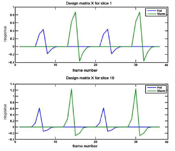

Refer to caption
Figure 14: Design matrix 𝑿isubscript𝑿𝑖\boldsymbol{X}_{i} for the first 40 frames, and slices Sisubscript𝑆𝑖S_{i}, with i=1𝑖1i=1 (top) and i=10𝑖10i=10 (bottom), obtained by fmridesign.m Matlab function through the convolution of our events matrix with the hrf model in Glover [1999].

Hilbert–valued fixed effect model fitting to FMRI data. A comparative study

The estimation results obtained with the implementation of the classical and Hilbert–valued linear model methodology are now compared. Specifically, in the classical case, from the linear model approach presented in Worsley et al. [2002], we consider a fixed–effect model fitting, in the case where the error term is an AR(1) process, ignoring spatial correlation across the voxels. In particular, the MatLab function fmrilm.m is implemented to fit model (44) to a single run of fMRI data, allowing for spatially varying temporal correlated errors. The parameters of the spatial varying AR(1) models (from voxel to voxel) are estimated from the sample autocorrelation of the residuals, obtained after estimation of the fixed effect parameter by ordinary least–squares, ignoring temporal correlation of the errors, at each voxel. This procedure could be iterated. That is, the estimated autocorrelation coefficient can be used to pre–whitening the data at each voxel. Hence, the fixed effect parameter is estimated by ordinary least-squares, from such data. This iterative estimation procedure can be repeated several times. However, as pointed out in Worsley et al. [2002], such iterations do not lead to a substantial improvement in practice. A variance reduction technique is then applied in Worsley et al. [2002] to the estimated autocorrelation coefficient (reduced bias sample autocorrelation), consisting of spatial smoothing of the sample autocorrelations. This technique reduces variability, although slightly increases the bias.

In this subsection, we also implement the approach introduced in Appendix 2, from the fMRI data set described in Appendix 5.1. As commented before, our approach presents the advantage of providing a continuous spatial description of the variation of the fixed effect parameters, as well as of the parameters characterizing the temporal correlated error term, with autoregressive dynamics. Furthermore, the spatial correlations are also incorporated to our functional statistical analysis, computed from the spatial autocovariance and cross-covariance kernels, respectively defining the operators R0subscript𝑅0R_{0} and R1,subscript𝑅1R_{1}, characterizing the functional dependence structure of the ARH(1) error term.

Functional fixed effect model fitting is independently performed at each slice Si,subscript𝑆𝑖S_{i}, for i=1,,16.𝑖116i=1,\dots,16. Specifically, for i=1,,16,𝑖116i=1,\dots,16, as commented before, a real-valued n×p,𝑛𝑝n\times p, with p=2,𝑝2p=2, fixed effect design matrix 𝐗isubscript𝐗𝑖\mathbf{X}_{i} is considered (see Appendix 5.1). The effects of the two different events studied are combined by the vector of functional fixed effect parameters

𝜷i()=[β1,i(),β2,i()]TH2.subscript𝜷𝑖superscriptsubscript𝛽1𝑖subscript𝛽2𝑖𝑇superscript𝐻2\boldsymbol{\beta}_{i}(\cdot)=[\beta_{1,i}(\cdot),\beta_{2,i}(\cdot)]^{T}\in H^{2}.

Here, H2superscript𝐻2H^{2} is the Hilbert space of 222–dimensional vector functions, whose components are square–integrable over the spatial rectangular grid considered at each slice. Furthermore, for i=1,,16,𝑖116i=1,\dots,16,

𝐘i()=[Y1,i(),,Yn,i()]Tsubscript𝐘𝑖superscriptsubscript𝑌1𝑖subscript𝑌𝑛𝑖𝑇\mathbf{Y}_{i}(\cdot)=[Y_{1,i}(\cdot),\dots,Y_{n,i}(\cdot)]^{T}

is the Hnsuperscript𝐻𝑛H^{n}–valued Gaussian fMRI data response, with n𝑛n representing the number of frames (n=64,𝑛64n=64, since the first 444 frames are removed because they do not represent steady–state images). In the computation of the generalized least–squares estimate of 𝜷,𝜷\boldsymbol{\beta}, the empirical matrices {𝚲^k,k=1,,TR}formulae-sequencesubscript^𝚲𝑘𝑘1𝑇𝑅\left\{\widehat{\boldsymbol{\Lambda}}_{k},\ k=1,\dots,TR\right\} are computed from the empirical covariance operators (19), where TR𝑇𝑅TR is selected according to the required conditions specified, in relation to the sample size n,𝑛n, in Bosq [2000] (see, in particular, [Bosq, 2000, pp. 101–102 and pp. 116–117], and Remark 3).

In the subsequent developments, in the results obtained by applying the Hilbert–valued multivariate fixed effect approach, we will distinguish between cases A and B, respectively corresponding to the projection into two and five empirical eigenvectors. For each one of the 161616 slices, the temporal and spatial averaged empirical quadratic errors, associated with the estimates of the response, computed with the fmrilm.m MatLab function, and with the proposed multivariate Hilbert–valued mixed effect approach, respectively denoted as EFMSE𝒀ifMRI𝐸𝐹𝑀𝑆subscript𝐸superscriptsubscript𝒀𝑖𝑓𝑀𝑅𝐼EFMSE_{\boldsymbol{Y}_{i}^{fMRI}} and EFMSE𝒀iH,𝐸𝐹𝑀𝑆subscript𝐸superscriptsubscript𝒀𝑖𝐻EFMSE_{\boldsymbol{Y}_{i}^{H}}, are displayed in Tables 1617.


Table 16: EFMSE𝒀ifMRI𝐸𝐹𝑀𝑆subscript𝐸superscriptsubscript𝒀𝑖𝑓𝑀𝑅𝐼EFMSE_{\boldsymbol{Y}_{i}^{fMRI}} and EFMSE𝒀iH𝐸𝐹𝑀𝑆subscript𝐸superscriptsubscript𝒀𝑖𝐻EFMSE_{\boldsymbol{Y}_{i}^{H}} for case A.
Slices Sisubscript𝑆𝑖S_{i} EFMSE𝒀ifMRI𝐸𝐹𝑀𝑆subscript𝐸superscriptsubscript𝒀𝑖𝑓𝑀𝑅𝐼EFMSE_{\boldsymbol{Y}_{i}^{fMRI}} EFMSE𝒀iH𝐸𝐹𝑀𝑆subscript𝐸superscriptsubscript𝒀𝑖𝐻EFMSE_{\boldsymbol{Y}_{i}^{H}}
1 2.417(10)32.417superscript1032.417(10)^{-}3 3.492(10)33.492superscript1033.492(10)^{-}3
2 3.051(10)33.051superscript1033.051(10)^{-}3 3.119(10)33.119superscript1033.119(10)^{-}3
3 4.293(10)34.293superscript1034.293(10)^{-}3 5.523(10)35.523superscript1035.523(10)^{-}3
4 6.666(10)36.666superscript1036.666(10)^{-}3 7.690(10)37.690superscript1037.690(10)^{-}3
5 8.986(10)38.986superscript1038.986(10)^{-}3 9.961(10)39.961superscript1039.961(10)^{-}3
6 8.462(10)38.462superscript1038.462(10)^{-}3 9.434(10)39.434superscript1039.434(10)^{-}3
7 1.108(10)21.108superscript1021.108(10)^{-}2 1.920(10)21.920superscript1021.920(10)^{-}2
8 1.720(10)21.720superscript1021.720(10)^{-}2 2.720(10)22.720superscript1022.720(10)^{-}2
9 1.499(10)21.499superscript1021.499(10)^{-}2 1.914(10)21.914superscript1021.914(10)^{-}2
10 1.036(10)21.036superscript1021.036(10)^{-}2 1.851(10)21.851superscript1021.851(10)^{-}2
11 1.308(10)21.308superscript1021.308(10)^{-}2 1.634(10)21.634superscript1021.634(10)^{-}2
12 1.302(10)21.302superscript1021.302(10)^{-}2 1.300(10)21.300superscript1021.300(10)^{-}2
13 7.850(10)37.850superscript1037.850(10)^{-}3 7.939(10)37.939superscript1037.939(10)^{-}3
14 6.640(10)36.640superscript1036.640(10)^{-}3 6.730(10)36.730superscript1036.730(10)^{-}3
15 3.511(10)33.511superscript1033.511(10)^{-}3 2.832(10)32.832superscript1032.832(10)^{-}3
16 2.771(10)32.771superscript1032.771(10)^{-}3 3.540(10)33.540superscript1033.540(10)^{-}3
Table 17: EFMSE𝒀ifMRI𝐸𝐹𝑀𝑆subscript𝐸superscriptsubscript𝒀𝑖𝑓𝑀𝑅𝐼EFMSE_{\boldsymbol{Y}_{i}^{fMRI}} and EFMSE𝒀iH𝐸𝐹𝑀𝑆subscript𝐸superscriptsubscript𝒀𝑖𝐻EFMSE_{\boldsymbol{Y}_{i}^{H}} for case B.
Slices Sisubscript𝑆𝑖S_{i} EFMSE𝒀ifMRI𝐸𝐹𝑀𝑆subscript𝐸superscriptsubscript𝒀𝑖𝑓𝑀𝑅𝐼EFMSE_{\boldsymbol{Y}_{i}^{fMRI}} EFMSE𝒀iH𝐸𝐹𝑀𝑆subscript𝐸superscriptsubscript𝒀𝑖𝐻EFMSE_{\boldsymbol{Y}_{i}^{H}}
1 2.417(10)32.417superscript1032.417(10)^{-}3 2.592(10)32.592superscript1032.592(10)^{-}3
2 3.051(10)33.051superscript1033.051(10)^{-}3 3.119(10)33.119superscript1033.119(10)^{-}3
3 4.293(10)34.293superscript1034.293(10)^{-}3 4.733(10)34.733superscript1034.733(10)^{-}3
4 6.666(10)36.666superscript1036.666(10)^{-}3 7.671(10)37.671superscript1037.671(10)^{-}3
5 8.986(10)38.986superscript1038.986(10)^{-}3 9.065(10)39.065superscript1039.065(10)^{-}3
6 8.462(10)38.462superscript1038.462(10)^{-}3 8.435(10)38.435superscript1038.435(10)^{-}3
7 1.108(10)21.108superscript1021.108(10)^{-}2 1.120(10)21.120superscript1021.120(10)^{-}2
8 1.720(10)21.720superscript1021.720(10)^{-}2 1.919(10)21.919superscript1021.919(10)^{-}2
9 1.499(10)21.499superscript1021.499(10)^{-}2 1.524(10)21.524superscript1021.524(10)^{-}2
10 1.036(10)21.036superscript1021.036(10)^{-}2 1.040(10)21.040superscript1021.040(10)^{-}2
11 1.308(10)21.308superscript1021.308(10)^{-}2 1.481(10)21.481superscript1021.481(10)^{-}2
12 1.302(10)21.302superscript1021.302(10)^{-}2 1.299(10)21.299superscript1021.299(10)^{-}2
13 7.849(10)37.849superscript1037.849(10)^{-}3 7.929(10)37.929superscript1037.929(10)^{-}3
14 6.640(10)36.640superscript1036.640(10)^{-}3 6.719(10)36.719superscript1036.719(10)^{-}3
15 3.511(10)33.511superscript1033.511(10)^{-}3 2.829(10)32.829superscript1032.829(10)^{-}3
16 2.771(10)32.771superscript1032.771(10)^{-}3 3.540(10)33.540superscript1033.540(10)^{-}3

It can be observed, in Tables 1617, that the performance of the two approaches is very similar. However, the advantage of the presented approach relies on the important dimension reduction it provides, since, as commented before, we have considered the truncations orders TR=2𝑇𝑅2TR=2 (Case A) and TR=5𝑇𝑅5TR=5 (Case B). Note that, for each slice, the parameter vector has dimension 2××(64×64),2\times\times(64\times 64), in the model fitted by fmrilm.m Matlab function. While the presented approach fits the functional projected model, that, for the the cases A and B studied, is defined in terms of a parameter vector 𝜷𝜷\boldsymbol{\beta} with dimension 2×2222\times 2 and 2×5,252\times 5, respectively. Furthermore, the iterative estimation method implemented in fmrilm.m requires several steps, repeated at each one of the 64×64646464\times 64 voxels in the 161616 slices (data pre–whitening, ordinary least-squares estimation of 𝜷𝜷\boldsymbol{\beta}, and AR(1) correlation coefficient estimation iterations, jointly with the spatial smoothing of the temporal correlation - reduced bias - parameter estimates).

For the slices 1,11, 5,55, 101010 and 15,1515, the temporal averaged (frames 555686868) estimated values of the response, applying fmrilm.m MatLab function, and the fixed effect model with ARH(1) error term, in cases A and B, are respectively displayed in Figures 1517. The corresponding empirical time-averaged quadratic errors are displayed in Figures 1820, respectively.


Refer to caption
Figure 15: Averaged in time (frames 555686868) estimated response values for slices 1,5,1015101,5,10 and 15,1515, obtained by applying fmrilm.m MatLab function.
Refer to caption
Figure 16: Averaged in time (frames 555686868) estimated response values for slices 1,5,1015101,5,10 and 15,1515, obtained by applying the fixed effect approach with ARH(1) error term, for case A.
Refer to caption
Figure 17: Averaged in time (frames 555686868) estimated response values for slices 1,5,1015101,5,10 and 15,1515, obtained by applying the fixed effect approach with ARH(1) error term, for case B.
Refer to caption
Figure 18: Averaged in time (frames 555686868) empirical errors for slices 1,5,1015101,5,10 and 15,1515, obtained by applying fmrilm.m MatLab function.
Refer to caption
Figure 19: Averaged in time (frames 555686868) empirical errors for slices 1,5,1015101,5,10 and 15,1515, obtained by applying the fixed effect approach with ARH(1) error term, for case A.
Refer to caption
Figure 20: Averaged in time (frames 555686868) empirical errors for slices 1,5,1015101,5,10 and 15,1515, obtained by applying the fixed effect approach with ARH(1) error term, for case B.

Significance test

We are interested in contrast the significance of the spatial varying parameter vector 𝜷𝜷\boldsymbol{\beta} combining the effects of the two stimulus considered on the overall brain, in its real-valued, and H2superscript𝐻2H^{2}-valued version. The F𝐹F statistic in the MatLab function fmrilm.m (fMRI linear model), computed, as before, from a single run of fMRI data, leads to the results reflected in Table 18, on the percentage of brain voxels, where the real–valued fixed effect model with AR(1) term is significative, for each one of the 161616 slices considered.


Table 18: Percentage of brain voxels per slice, where the real-valued fixed effect model with AR(1) error term, fitted by fmrilm.m MatLab function, is significative.
S𝑆S % voxels with rejection of H0subscript𝐻0H_{0}
111 99.927%percent99.92799.927\%
222 99.927%percent99.92799.927\%
333 99.707%percent99.70799.707\%
444 99.902%percent99.90299.902\%
555 99.805%percent99.80599.805\%
666 99.951%percent99.95199.951\%
777 99.927%percent99.92799.927\%
888 99.976%percent99.97699.976\%
999 99.805%percent99.80599.805\%
101010 99.951%percent99.95199.951\%
111111 99.951%percent99.95199.951\%
121212 99.902%percent99.90299.902\%
131313 99.878%percent99.87899.878\%
141414 99.951%percent99.95199.951\%
151515 99.951%percent99.95199.951\%
161616 100%percent100100\%

As described in Appendix 3, for each slice, i.e., for i=1,,16,𝑖116i=1,\dots,16, the value of the conditional chi–squared test statistics T𝒉,subscript𝑇𝒉T_{\boldsymbol{h}}, in equation (30), is computed, from four realizations of a Gaussian random function 𝒉,𝒉\boldsymbol{h}, generated from a Gaussian random field ξ,𝜉\xi, satisfying equation (LABEL:A4:eqdlrect) on the rectangle containing each brain slice. As before, the functional response sample size at each slice is 64,6464, since the first four frames are discarded. It can be observed, in the numerical results displayed in Table 19, for TR=16,𝑇𝑅16TR=16, and in Table 20, for TR=4,𝑇𝑅4TR=4, that the null hypothesis is rejected, in most of the random directions in all the brain slices; i.e., the functional fixed effect model with ARH(1) error term is significative for α=0.05.𝛼0.05\alpha=0.05. Note that a very few p𝑝p–values are slightly larger than α=0.05,𝛼0.05\alpha=0.05, with very small difference, that could be produced by the numerical errors accumulated, due to the presence of small values to be inverted. Thus, we can conclude the suitability of our approach, to combine the effects of the scans hot stimulus, and the scans warm stimulus, in a functional spatially continuous framework.


Table 19: p𝑝p-values for T𝒉subscript𝑇𝒉T_{\boldsymbol{h}} computed at the 161616 slices, considering four random directions, for TR=16𝑇𝑅16TR=16.
S𝑆S D1subscript𝐷1D_{1} D2subscript𝐷2D_{2} D3subscript𝐷3D_{3} D4subscript𝐷4D_{4}
111 00 00 0.0820.0820.082 0.0230.0230.023
222 0.590(10)20.590superscript1020.590(10)^{-2} 00 00 00
333 0.0180.0180.018 0.0660.0660.066 0.0490.0490.049 0.0300.0300.030
444 00 00 00 0.170(10)100.170superscript10100.170(10)^{-10}
555 00 0.0260.0260.026 00 00
666 00 00 00 00
777 0.710(10)70.710superscript1070.710(10)^{-7} 00 00 00
888 00 0.0060.0060.006 00 00
999 0.0490.0490.049 00 00 0.0230.0230.023
101010 0.390(10)70.390superscript1070.390(10)^{-7} 0.0310.0310.031 00 00
111111 0.0040.0040.004 0.0060.0060.006 0.660(10)60.660superscript1060.660(10)^{-6} 0.0520.0520.052
121212 0.0460.0460.046 00 00 0.0340.0340.034
131313 0.340(10)70.340superscript1070.340(10)^{-7} 0.0280.0280.028 00 0.440(10)30.440superscript1030.440(10)^{-3}
141414 00 0.180(10)60.180superscript1060.180(10)^{-6} 0.0210.0210.021 0.0500.0500.050
151515 00 0.140(10)70.140superscript1070.140(10)^{-7} 0.0440.0440.044 0.0520.0520.052
161616 0.110(10)40.110superscript1040.110(10)^{-4} 0.230(10)70.230superscript1070.230(10)^{-7} 00 00

Table 20: p𝑝p-values for T𝒉subscript𝑇𝒉T_{\boldsymbol{h}} computed at the 161616 slices, considering four random directions, for TR=4𝑇𝑅4TR=4.
S𝑆S D1subscript𝐷1D_{1} D2subscript𝐷2D_{2} D3subscript𝐷3D_{3} D4subscript𝐷4D_{4}
111 00 0.0510.0510.051 0.0710.0710.071 0.0110.0110.011
222 0.880(10)40.880superscript1040.880(10)^{-4} 00 00 00
333 0.0670.0670.067 0.0340.0340.034 00 0.0370.0370.037
444 00 0.250(10)40.250superscript1040.250(10)^{-4} 0.110(10)40.110superscript1040.110(10)^{-4} 0.0160.0160.016
555 0.370(10)60.370superscript1060.370(10)^{-6} 00 0.280(10)60.280superscript1060.280(10)^{-6} 00
666 0.0010.0010.001 00 00 0.220(10)40.220superscript1040.220(10)^{-4}
777 0.0640.0640.064 0.0340.0340.034 0.0070.0070.007 0.0440.0440.044
888 0.0720.0720.072 0.0790.0790.079 0.0350.0350.035 00
999 0.220(10)50.220superscript1050.220(10)^{-5} 0.470(10)40.470superscript1040.470(10)^{-4} 0.0040.0040.004 0.220(10)90.220superscript1090.220(10)^{-9}
101010 00 0.120(10)30.120superscript1030.120(10)^{-3} 0.370(10)40.370superscript1040.370(10)^{-4} 0.970(10)70.970superscript1070.970(10)^{-7}
111111 0.0810.0810.081 0.0580.0580.058 00 00
121212 0.870(10)40.870superscript1040.870(10)^{-4} 00 00 0.0360.0360.036
131313 0.760(10)30.760superscript1030.760(10)^{-3} 00 00 0.370(10)30.370superscript1030.370(10)^{-3}
141414 0.210(10)60.210superscript1060.210(10)^{-6} 00 00 0.0370.0370.037
151515 00 0.650(10)40.650superscript1040.650(10)^{-4} 0.0320.0320.032 00
161616 0.540(10)60.540superscript1060.540(10)^{-6} 00 00 0.520(10)30.520superscript1030.520(10)^{-3}

Comparing results in Tables 1820, we can conclude that both methodologies, the one presented in Worsley et al. [2002], and the functional approach introduced here, lead to similar results regarding the significance of the models they propose, respectively based on spatial varying real–valued multiplicative coefficients with AR(1) error term, and Hilbert–valued coefficients with ARH(1) error term.

6 Conclusions

As shown in the simulation study, the boundary conditions affect the decay velocity at the boundary of the covariance kernels, defining the functional entries of the matrix covariance operator of the error term. Thus, the dependence range of the error components is directly affected by the boundary conditions. A better performance of the generalized least–squares estimator of the parameter vector 𝜷𝜷\boldsymbol{\beta} is observed, when a fast continuous decay is displayed by the error covariance kernels close to the boundary, as it is observed in the circular domains. Furthermore, in the simulation study undertaken, and in the real–data problem addressed, a good performance of the computed generalized least–squares estimator, and of the test statistics is observed for low truncation orders. Thus, an important dimension reduction is achieved with the presented approach. Summarizing, the proposed approach allows the incorporation of temporal and spatial correlations in the analysis, with an important dimension reduction.

The derivation of similar results under alternative boundary conditions like Neumann and Robin boundary conditions constitutes an open research problem (see, for example, Grebenkov and Nguyen [2013]). Another important research problem is to address the same analysis under a slow decay of the error covariance kernels at the boundary (see, for example, Frías et al. [2017], Jiang [2012, 2016], Tong [2011], beyond the Gaussian context).

7 Supplementary Material

The eigenvectors and eigenvalues of the Dirichlet negative Laplacian operator on the regular domains defined by the rectangle, disk and circular sector are described here (see, for example, Grebenkov and Nguyen [2013]). It is well–known that the negative Laplacian operator (𝚫D)subscript𝚫𝐷\left(-\boldsymbol{\Delta}_{D}\right) on a regular bounded open domain D2,𝐷superscript2D\subset\mathbb{R}^{2}, with Dirichlet boundary conditions, is given by

𝚫D(f)(x1,x2)=2x12f(x1,x2)2x22f(x1,x2),f(x1,x2)=0,(x1,x2)D,D2,formulae-sequencesubscript𝚫𝐷𝑓subscript𝑥1subscript𝑥2superscript2superscriptsubscript𝑥12𝑓subscript𝑥1subscript𝑥2superscript2superscriptsubscript𝑥22𝑓subscript𝑥1subscript𝑥2formulae-sequence𝑓subscript𝑥1subscript𝑥20formulae-sequencesubscript𝑥1subscript𝑥2𝐷𝐷superscript2-\boldsymbol{\Delta}_{D}(f)(x_{1},x_{2})=-\frac{\partial^{2}}{\partial x_{1}^{2}}f(x_{1},x_{2})-\frac{\partial^{2}}{\partial x_{2}^{2}}f(x_{1},x_{2}),\quad f(x_{1},x_{2})=0,\quad(x_{1},x_{2})\in\partial D,\quad D\subseteq\mathbb{R}^{2},

where D𝐷\partial D is the boundary of D.𝐷D. In the subsequent development, we will denote by {ϕk,k1}subscriptitalic-ϕ𝑘𝑘1\left\{\phi_{k},\ k\geq 1\right\} and {λk(𝚫D),k1}subscript𝜆𝑘subscript𝚫𝐷𝑘1\left\{\lambda_{k}(-\boldsymbol{\Delta}_{D}),\ k\geq 1\right\} the respective eigenvectors and eigenvalues of (𝚫D),subscript𝚫𝐷\left(-\boldsymbol{\Delta}_{D}\right), that satisfy

𝚫Dϕk(𝐱)subscript𝚫𝐷subscriptitalic-ϕ𝑘𝐱\displaystyle-\boldsymbol{\Delta}_{D}\phi_{k}\left(\mathbf{x}\right) =\displaystyle= λk(𝚫D)ϕk(𝐱)(𝐱D2),subscript𝜆𝑘subscript𝚫𝐷subscriptitalic-ϕ𝑘𝐱𝐱𝐷superscript2\displaystyle\lambda_{k}(-\boldsymbol{\Delta}_{D})\phi_{k}\left(\mathbf{x}\right)\leavevmode\nobreak\ \left(\mathbf{x}\in D\subseteq\mathbb{R}^{2}\right),
ϕk(𝐱)subscriptitalic-ϕ𝑘𝐱\displaystyle\phi_{k}\left(\mathbf{x}\right) =\displaystyle= 0(𝐱D),k1,0𝐱𝐷for-all𝑘1\displaystyle 0\leavevmode\nobreak\ \left(\mathbf{x}\in\partial D\right),\leavevmode\nobreak\ \forall k\geq 1,

for D𝐷D being one of the following three domains:

D1=i=12[ai,bi],D2={𝐱2:R0<𝐱<R},formulae-sequencesubscript𝐷1superscriptsubscriptproduct𝑖12subscript𝑎𝑖subscript𝑏𝑖subscript𝐷2conditional-set𝐱superscript2subscript𝑅0norm𝐱𝑅D_{1}=\prod_{i=1}^{2}\left[a_{i},b_{i}\right],\quad D_{2}=\left\{\mathbf{x}\in\mathbb{R}^{2}:\leavevmode\nobreak\ R_{0}<\|\mathbf{x}\|<R\right\},

and

D3={𝐱2:R0<𝐱<R,and 0<φ<πθ}.subscript𝐷3conditional-set𝐱superscript2formulae-sequencesubscript𝑅0norm𝐱𝑅and 0𝜑𝜋𝜃D_{3}=\left\{\mathbf{x}\in\mathbb{R}^{2}:\leavevmode\nobreak\ R_{0}<\|\mathbf{x}\|<R,\ \mbox{and}\ 0<\varphi<\pi\theta\right\}.

Eigenelements of Dirichlet negative Laplacian operator on rectangles

Let us first consider domain

D1=i=12[ai,bi].subscript𝐷1superscriptsubscriptproduct𝑖12subscript𝑎𝑖subscript𝑏𝑖D_{1}=\prod_{i=1}^{2}\left[a_{i},b_{i}\right].

The eigenvectors {ϕ𝐤,𝐤2}subscriptitalic-ϕ𝐤𝐤subscriptsuperscript2\left\{\phi_{\mathbf{k}},\ \mathbf{k}\in\mathbb{N}^{2}_{*}\right\} and eigenvalues {λ𝐤(𝚫D1),𝐤2}subscript𝜆𝐤subscript𝚫subscript𝐷1𝐤subscriptsuperscript2\left\{\lambda_{\mathbf{k}}(-\boldsymbol{\Delta}_{D_{1}}),\ \mathbf{k}\in\mathbb{N}^{2}_{*}\right\} of 𝚫D1subscript𝚫subscript𝐷1-\boldsymbol{\Delta}_{D_{1}} are given by (see Grebenkov and Nguyen [2013]):

ϕ𝐤(𝐱)subscriptitalic-ϕ𝐤𝐱\displaystyle\phi_{\mathbf{k}}\left(\mathbf{x}\right) =\displaystyle= ϕk1(1)(x1)ϕk2(2)(x2),λ𝐤=λk1(1)+λk2(2),superscriptsubscriptitalic-ϕsubscript𝑘11subscript𝑥1superscriptsubscriptitalic-ϕsubscript𝑘22subscript𝑥2subscript𝜆𝐤superscriptsubscript𝜆subscript𝑘11superscriptsubscript𝜆subscript𝑘22\displaystyle\phi_{k_{1}}^{(1)}\left(x_{1}\right)\phi_{k_{2}}^{(2)}\left(x_{2}\right),\leavevmode\nobreak\ \lambda_{\mathbf{k}}=\lambda_{k_{1}}^{(1)}+\lambda_{k_{2}}^{(2)},
ϕki(i)(xi)superscriptsubscriptitalic-ϕsubscript𝑘𝑖𝑖subscript𝑥𝑖\displaystyle\phi_{k_{i}}^{(i)}\left(x_{i}\right) =\displaystyle= sin(πkixili),xi[ai,bi],i=1,2,formulae-sequence𝜋subscript𝑘𝑖subscript𝑥𝑖subscript𝑙𝑖subscript𝑥𝑖subscript𝑎𝑖subscript𝑏𝑖𝑖12\displaystyle\sin\left(\frac{\pi k_{i}x_{i}}{l_{i}}\right),\quad x_{i}\in\left[a_{i},b_{i}\right],\leavevmode\nobreak\ i=1,2,
λki(i)superscriptsubscript𝜆subscript𝑘𝑖𝑖\displaystyle\lambda_{k_{i}}^{(i)} =\displaystyle= π2ki2li2,ki1,i=1,2,formulae-sequencesuperscript𝜋2superscriptsubscript𝑘𝑖2superscriptsubscript𝑙𝑖2subscript𝑘𝑖1𝑖12\displaystyle\frac{\pi^{2}k_{i}^{2}}{l_{i}^{2}},\quad k_{i}\geq 1,\leavevmode\nobreak\ i=1,2,

where li=biai,subscript𝑙𝑖subscript𝑏𝑖subscript𝑎𝑖l_{i}=b_{i}-a_{i}, for i=1,2.𝑖12i=1,2.

Eigenelements of Dirichlet negative Laplacian operator on disks

In general, for the circular annulus

D~2={𝐱2:R0<𝐱<R},subscript~𝐷2conditional-set𝐱superscript2subscript𝑅0norm𝐱𝑅\widetilde{D}_{2}=\left\{\mathbf{x}\in\mathbb{R}^{2}:\leavevmode\nobreak\ R_{0}<\|\mathbf{x}\|<R\right\},

its rotation symmetry allows us to define 𝚫D~2subscript𝚫subscript~𝐷2-\boldsymbol{\Delta}_{\widetilde{D}_{2}} in polar coordinates as

𝚫D~2=2r21rr1r22φ2,x1=rcosφ,x2=rsinφ.formulae-sequencesubscript𝚫subscript~𝐷2superscript2superscript𝑟21𝑟𝑟1superscript𝑟2superscript2superscript𝜑2formulae-sequencesubscript𝑥1𝑟𝜑subscript𝑥2𝑟𝜑-\boldsymbol{\Delta}_{\widetilde{D}_{2}}=-\frac{\partial^{2}}{\partial r^{2}}-\frac{1}{r}\frac{\partial}{\partial r}-\frac{1}{r^{2}}\frac{\partial^{2}}{\partial\varphi^{2}},\quad x_{1}=r\cos\varphi,\leavevmode\nobreak\ x_{2}=r\sin\varphi.

The application of variable separation method then leads to the following explicit formula of its eigenfunctions (see, for example, Grebenkov and Nguyen [2013])

ϕkhl(r,φ)=[Jk(αkhr/R)+ckhYk(αkhr/R)]×Ck(l),subscriptitalic-ϕ𝑘𝑙𝑟𝜑delimited-[]subscript𝐽𝑘subscript𝛼𝑘𝑟𝑅subscript𝑐𝑘subscript𝑌𝑘subscript𝛼𝑘𝑟𝑅subscript𝐶𝑘𝑙\phi_{khl}\left(r,\varphi\right)=\left[J_{k}\left(\alpha_{kh}r/R\right)+c_{kh}Y_{k}\left(\alpha_{kh}r/R\right)\right]\times C_{k}\left(l\right), (47)

with

Ck(l)={cos(kφ) l=1,sin(kφ) l=2 (k0),subscript𝐶𝑘𝑙cases𝑐𝑜𝑠𝑘𝜑 l=1𝑠𝑖𝑛𝑘𝜑 l=2 𝑘0C_{k}(l)=\left\{\begin{array}[]{l}cos\left(k\varphi\right)\text{ l=1},\\ sin\left(k\varphi\right)\text{ l=2 }\left(k\neq 0\right),\end{array}\right.

where {Jk(z)}subscript𝐽𝑘𝑧\{J_{k}\left(z\right)\} and {Yk(z)}subscript𝑌𝑘𝑧\{Y_{k}\left(z\right)\} are the Bessel functions of order k𝑘k of first and second kind, respectively,

{λkh(𝚫D~2)=αkh2/R2}subscript𝜆𝑘subscript𝚫subscript~𝐷2superscriptsubscript𝛼𝑘2superscript𝑅2\{\lambda_{kh}\left(-\boldsymbol{\Delta}_{\widetilde{D}_{2}}\right)=\alpha_{kh}^{2}/R^{2}\}

are the corresponding eigenvalues, and the sets {αk,h,k1,h=1,,M(k)}formulae-sequencesubscript𝛼𝑘𝑘11𝑀𝑘\left\{\alpha_{k,h},\ k\geq 1,\leavevmode\nobreak\ h=1,\dots,M(k)\right\} and {ck,h,k1,h=1,,M(k)}formulae-sequencesubscript𝑐𝑘𝑘11𝑀𝑘\left\{c_{k,h},\ k\geq 1,\leavevmode\nobreak\ h=1,\dots,M(k)\right\} are defined from the boundary conditions at r=R𝑟𝑅r=R and r=R0.𝑟subscript𝑅0r=R_{0}.

If we focus on domain D2,subscript𝐷2D_{2}, the disk, i.e., R0=0subscript𝑅00R_{0}=0, the coefficients {ck,h,k1,h=1,,M(k)}formulae-sequencesubscript𝑐𝑘𝑘11𝑀𝑘\left\{c_{k,h},\ k\geq 1,\leavevmode\nobreak\ h=1,\dots,M(k)\right\} are set to 0.00. The eigenfunctions then adopt the following expression:

ϕkhl(r,φ)subscriptitalic-ϕ𝑘𝑙𝑟𝜑\displaystyle\phi_{khl}\left(r,\varphi\right) =\displaystyle= Jk(αkhr/R)Ck(l),l=1,2,formulae-sequencesubscript𝐽𝑘subscript𝛼𝑘𝑟𝑅subscript𝐶𝑘𝑙𝑙12\displaystyle J_{k}\left(\alpha_{kh}r/R\right)C_{k}(l),\quad l=1,2,

with eigenvalues

λkh(𝚫D2)=αkh2R2,k1,h=1,,M(k),formulae-sequencesubscript𝜆𝑘subscript𝚫subscript𝐷2superscriptsubscript𝛼𝑘2superscript𝑅2formulae-sequence𝑘11𝑀𝑘\lambda_{kh}\left(-\boldsymbol{\Delta}_{D_{2}}\right)=\frac{\alpha_{kh}^{2}}{R^{2}},\quad k\geq 1,\leavevmode\nobreak\ h=1,\dots,M(k),

where {αk,h,h=1,,M(k)}formulae-sequencesubscript𝛼𝑘1𝑀𝑘\left\{\alpha_{k,h},\ h=1,\dots,M(k)\right\} are the M(k)𝑀𝑘M(k) positive roots of the Bessel function Jk(z)subscript𝐽𝑘𝑧J_{k}\left(z\right) of order k.𝑘k. Note that we can also consider truncation at parameter M(k)𝑀𝑘M(k) for k1,𝑘1k\geq 1, since this parameter increases with the increasing of the radius R.𝑅R.

Eigenelements of Dirichlet negative Laplacian operator on circular sectors

Lastly, we consider domain D3,subscript𝐷3D_{3}, the circular sector of radius R𝑅R and angle 0<φ<πθ.0𝜑𝜋𝜃0<\varphi<\pi\theta. The eigenvectors and eigenvalues are given by the following expression (see, for example, Grebenkov and Nguyen [2013]):

ϕkh(r,φ)subscriptitalic-ϕ𝑘𝑟𝜑\displaystyle\phi_{kh}\left(r,\varphi\right) =\displaystyle= Jk/θ(αkhr/R)sin(kφ/θ),r[0,R],subscript𝐽𝑘𝜃subscript𝛼𝑘𝑟𝑅𝑘𝜑𝜃𝑟0𝑅\displaystyle J_{k/\theta}\left(\alpha_{kh}r/R\right)\sin\left(k\varphi/\theta\right),\quad r\in\left[0,R\right],
λkh(𝚫D3)subscript𝜆𝑘subscript𝚫subscript𝐷3\displaystyle\lambda_{kh}\left(-\boldsymbol{\Delta}_{D_{3}}\right) =\displaystyle= αkh2R2,k1,h=1,,M(k),formulae-sequencesuperscriptsubscript𝛼𝑘2superscript𝑅2𝑘11𝑀𝑘\displaystyle\frac{\alpha_{kh}^{2}}{R^{2}},\ k\geq 1,\leavevmode\nobreak\ h=1,\dots,M(k),

with M(k)𝑀𝑘M(k) and {αk,h,k1,h=1,,M(k)}formulae-sequencesubscript𝛼𝑘𝑘11𝑀𝑘\left\{\alpha_{k,h},\ k\geq 1,\leavevmode\nobreak\ h=1,\dots,M(k)\right\} being given as in the previous section.

Asymptotic behavior of eigenvalues

7.4.1 The rectangle

The functional data sets generated in Appendix 4 must have a covariance matrix operator with functional entries (operators) in the trace class. We then apply the results in Widom [1963] to study the asymptotic order of eigenvalues of the integral equation

2V1/2(𝐭)lεi(𝐭𝐬)V1/2(𝐬)f(𝐬)𝑑𝐬=λf(𝐭).subscriptsuperscript2superscript𝑉12𝐭subscript𝑙subscript𝜀𝑖𝐭𝐬superscript𝑉12𝐬𝑓𝐬differential-d𝐬𝜆𝑓𝐭\displaystyle\int_{\mathbb{R}^{2}}V^{1/2}(\mathbf{t})l_{\varepsilon_{i}}(\mathbf{t}-\mathbf{s})V^{1/2}(\mathbf{s})f(\mathbf{s})d\mathbf{s}=\lambda f(\mathbf{t}).

In our case, V𝑉V is the indicator function on the rectangle, i.e., on domain D1,subscript𝐷1D_{1}, and lεisubscript𝑙subscript𝜀𝑖l_{\varepsilon_{i}} is the covariance kernel defining the square root

Rεiεi1/2=fi(𝚫D1)=(𝚫D1)(dγi),γi(0,d/2),formulae-sequencesubscriptsuperscript𝑅12subscript𝜀𝑖subscript𝜀𝑖subscript𝑓𝑖subscript𝚫subscript𝐷1superscriptsubscript𝚫subscript𝐷1𝑑subscript𝛾𝑖subscript𝛾𝑖0𝑑2R^{1/2}_{\varepsilon_{i}\varepsilon_{i}}=f_{i}(-\boldsymbol{\Delta}_{D_{1}})=(-\boldsymbol{\Delta}_{D_{1}})^{-(d-\gamma_{i})},\quad\gamma_{i}\in(0,d/2),

of the autocovariance operator of the Hilbert-valued error component {εi,i=1,,n},formulae-sequencesubscript𝜀𝑖𝑖1𝑛\left\{\varepsilon_{i},\ i=1,\dots,n\right\}, with

Rεiεi=Rεiεi1/2Rεiεi1/2.subscript𝑅subscript𝜀𝑖subscript𝜀𝑖subscriptsuperscript𝑅12subscript𝜀𝑖subscript𝜀𝑖subscriptsuperscript𝑅12subscript𝜀𝑖subscript𝜀𝑖R_{\varepsilon_{i}\varepsilon_{i}}=R^{1/2}_{\varepsilon_{i}\varepsilon_{i}}R^{1/2}_{\varepsilon_{i}\varepsilon_{i}}.

Note that with the choice made of functions V𝑉V and {lεi,i=1,,n},formulae-sequencesubscript𝑙subscript𝜀𝑖𝑖1𝑛\left\{l_{\varepsilon_{i}},\ i=1,\dots,n\right\}, the conditions assumed in Widom [1963] are satisfied. In particular, the following asymptotic holds:

λk(Rεiεi1/2)=𝒪(k2(dγi)/d),k,i=1,,n,formulae-sequencesubscript𝜆𝑘superscriptsubscript𝑅subscript𝜀𝑖subscript𝜀𝑖12𝒪superscript𝑘2𝑑subscript𝛾𝑖𝑑formulae-sequence𝑘𝑖1𝑛\lambda_{k}(R_{\varepsilon_{i}\varepsilon_{i}}^{1/2})=\mathcal{O}(k^{-2(d-\gamma_{i})/d}),\quad k\longrightarrow\infty,\quad i=1,\dots,n,

(see [Widom, 1963, p. 279, Eq. (2)]). Also, in general, the eigenvalues of the Dirichlet negative Laplacian operator on a regular bounded open domain D𝐷D satisfy

γk(ΔD)4π(Γ(1+d2))2/d|D|2/dk2/d,k.formulae-sequencesimilar-tosubscript𝛾𝑘subscriptΔ𝐷4𝜋superscriptΓ1𝑑22𝑑superscript𝐷2𝑑superscript𝑘2𝑑𝑘\gamma_{k}(-\Delta_{D})\sim 4\pi\frac{\left(\Gamma\left(1+\frac{d}{2}\right)\right)^{2/d}}{|D|^{2/d}}k^{2/d},\quad k\longrightarrow\infty.

7.4.2 Asymptotic behavior of zeros of Bessel functions.

As before, Jk(z)subscript𝐽𝑘𝑧J_{k}\left(z\right) denotes the Bessel function of the first kind of order k.𝑘k. Let {jk,h,h=1,,M(k)}formulae-sequencesubscript𝑗𝑘1𝑀𝑘\left\{j_{k,h},\ h=1,\dots,M(k)\right\} be its M(k)𝑀𝑘M(k) roots. In Elbert [2001], Olver [1951, 1952], it is shown that, for a fixed hh and large k𝑘k, the Olver’s expansion holds

jkhk+δhk1/3+𝒪(k1/3),k.formulae-sequencesimilar-to-or-equalssubscript𝑗𝑘𝑘subscript𝛿superscript𝑘13𝒪superscript𝑘13𝑘j_{kh}\simeq k+\delta_{h}k^{1/3}+\mathcal{O}(k^{-1/3}),\quad k\rightarrow\infty.

On the other hand, for fixed k𝑘k and large hh, the McMahon’s expansion also is satisfied (see, for example, Watson [1966])

jkhπ(h+k/21/4)+𝒪(h1),h.formulae-sequencesimilar-to-or-equalssubscript𝑗𝑘𝜋𝑘214𝒪superscript1j_{kh}\simeq\pi\left(h+k/2-1/4\right)+\mathcal{O}(h^{-1}),\quad h\rightarrow\infty.

These results will be applied in Appendix 4, in the definition of the eigenvalues of the covariance operators {𝑹εiεi,i=1,,n},formulae-sequencesubscript𝑹subscript𝜀𝑖subscript𝜀𝑖𝑖1𝑛\left\{\boldsymbol{R}_{\varepsilon_{i}\varepsilon_{i}},\ i=1,\dots,n\right\}, on the disk and circular sector, to ensure their rapid decay to zero, characterizing the trace operator class.

Acknowledgments

This work has been supported in part by project MTM2015–71839–P (co-funded by Feder funds), of the DGI, MINECO, Spain.

References

  • Abramovich and Angelini [2006] \NAT@biblabelnumAbramovich and Angelini 2006 Abramovich, F. ; Angelini, C.: Testing in mixed-effects FANOVA models. J. Statist. Plann. Inference 136 (2006), pp. 4326–4348. – DOI: doi.org/10.1016/j.jspi.2005.06.002
  • Abramovich et al. [2004] \NAT@biblabelnumAbramovich et al. 2004 Abramovich, F. ; Antoniadis, A. ; Sapatinas, T. ; Vidakovic, B.: Optimal testing in functional analysis of variance models. Int. J. Wavelets Multiresolut. Inf. Process. 2 (2004), pp. 323–349. – URL http://citeseerx.ist.psu.edu/viewdoc/download?doi=10.1.1.140.6784&rep=rep1&type=pdf
  • Angelini et al. [2003] \NAT@biblabelnumAngelini et al. 2003 Angelini, C. ; Canditiis, D. D. ; Leblanc, F.: Wavelet regression estimation in nonparametric mixed effect models. J. Multivariate Anal. 85 (2003), pp. 267–291. – DOI: doi.org/10.1016/S0047-259X(02)00055-6
  • Antoniadis and Sapatinas [2007] \NAT@biblabelnumAntoniadis and Sapatinas 2007 Antoniadis, A. ; Sapatinas, T.: Estimation and inference in functional mixed-effects models. Comput. Statist. Data Anal. 51 (2007), pp. 4793–4813. – DOI: doi.org/10.1016/j.csda.2006.09.038
  • Banerjee et al. [2004] \NAT@biblabelnumBanerjee et al. 2004 Banerjee, S. ; Carlin, B. P. ; Gelfand, A. E.: Hierarchical Modeling and Analysis for Spatial Data. Chapman and Hall, London, 2004. – ISBN 9781584884101
  • Besag [1986] \NAT@biblabelnumBesag 1986 Besag, J.: On the statistical analysis of dirty pictures. J. R. Stat. Soc. Ser. B Stat. Methodol. 48 (1986), pp. 259–302. – URL www.jstor.org/stable/2345426
  • Bosq [2000] \NAT@biblabelnumBosq 2000 Bosq, D.: Linear Processes in Function Spaces. Springer, New York, 2000. – ISBN 9781461211549
  • Bosq [2007] \NAT@biblabelnumBosq 2007 Bosq, D.: General linear processes in Hilbert spaces and prediction. J. Statist. Plann. Inference 137 (2007), pp. 879–894. – DOI: doi.org/10.1016/j.jspi.2006.06.014
  • Bulaevskaya and Oehlert [2007] \NAT@biblabelnumBulaevskaya and Oehlert 2007 Bulaevskaya, V. L. ; Oehlert, G. W.: A penalized likelihood approach to magnetic resonance image reconstruction. Stat. Med. 26 (2007), pp. 352–374. – DOI: doi.org/10.1002/sim.2545
  • Cai and Hall [2006] \NAT@biblabelnumCai and Hall 2006 Cai, T. ; Hall, P.: Prediction in functional linear regression. Ann. Statist. 34 (2006), pp. 2159–2179. – DOI: doi.org/10.1214/009053606000000830
  • Cardot et al. [2003] \NAT@biblabelnumCardot et al. 2003 Cardot, H. ; Ferraty, F. ; Sarda, P.: Spline estimators for the functional linear model. Statist. Sinica 13 (2003), pp. 571–591. – DOI: doi.org/10.1016/j.jmva.2006.10.004
  • Cardot and Sarda [2011] \NAT@biblabelnumCardot and Sarda 2011 Cardot, H. ; Sarda, P.: Functional linear regression. In: Ferraty, F., Romain, Y. (Eds.) The Oxford Handbook of Functional Data Analysis. Oxford University Press, Oxford (2011), pp. 21–46
  • Chiou et al. [2004] \NAT@biblabelnumChiou et al. 2004 Chiou, J. M. ; Müller, H. G. ; Wang, J. L.: Functional response models. Statist. Sinica 14 (2004), pp. 675–693. – URL http://anson.ucdavis.edu/~mueller/fdr9-15.pdf
  • Christensen and Yetkin [2005] \NAT@biblabelnumChristensen and Yetkin 2005 Christensen, W. F. ; Yetkin, F. Z.: Spatio-temporal analysis of auditory cortex activation as detected with silent event related fMRI. Stat. Med. 24 (2005), pp. 2539–2556. – DOI: doi.org/10.1002/sim.2111
  • Chung et al. [2005] \NAT@biblabelnumChung et al. 2005 Chung, K. K. ; Robbins, S. M. ; Dalton, K. M. ; Davidson, R. J. ; Alexander, A. L. ; Evans, A. C.: Cortical thickness analysis in autism with heat. Neuroimage 25 (2005), pp. 1256–1265. – DOI: doi.org/10.1016/j.neuroimage.2004.12.052
  • Crambes et al. [2009] \NAT@biblabelnumCrambes et al. 2009 Crambes, C. ; Kneip, A. ; Sarda, P.: Smoothing splines estimators for functional linear regression. Ann. Statist. 37 (2009), pp. 35–72. – DOI: doi.org/10.1214/07-AOS563
  • Cuesta-Albertos and Febrero-Bande [2010] \NAT@biblabelnumCuesta-Albertos and Febrero-Bande 2010 Cuesta-Albertos, J. A. ; Febrero-Bande, M. F.: Multiway ANOVA for functional data. Test 19 (2010), pp. 537–557. – DOI: doi.org/10.1007/s11749-010-0185-3
  • Cuesta-Albertos et al. [2007] \NAT@biblabelnumCuesta-Albertos et al. 2007 Cuesta-Albertos, J. A. ; Fraiman, R. ; Ransford, T.: A sharp form of the Cramér–Wold theorem. J. Theoret. Probab. 20 (2007), pp. 201–209. – DOI: doi.org/10.1007/s10959-007-0060-7
  • Cuevas et al. [2002] \NAT@biblabelnumCuevas et al. 2002 Cuevas, A. ; Febrero, M. ; Fraiman, R.: Linear functional regression: the case of fixed design and functional response. Canad. J. Statist. 30 (2002), pp. 285–300. – DOI: doi.org/10.2307/3315952
  • Cuevas et al. [2004] \NAT@biblabelnumCuevas et al. 2004 Cuevas, A. ; Febrero-Bande, M. F. ; Fraiman, R.: An ANOVA test for functional data. Comput. Statist. Data Anal. 47 (2004), pp. 111–122. – DOI: doi.org/10.1016/j.csda.2003.10.021
  • Delzell et al. [2012] \NAT@biblabelnumDelzell et al. 2012 Delzell, D. A. P. ; Gunst, R. F. ; Schucany, W. R. ; Carmack, P. S. ; Lin, Q. ; Spence, J. S. ; Haley, R. W.: Key properties of D-optimal designs for event-related functional MRI experiments with applications to nonlinear models. Stat. Med. 31 (2012), pp. 3907–3920. – DOI: doi.org/10.1002/sim.5449
  • Dette and Derbort [2001] \NAT@biblabelnumDette and Derbort 2001 Dette, H. ; Derbort, S.: Analysis of variance in nonparametric regression models. J. Multivariate Anal. 76 (2001), pp. 110–137. – DOI: doi.org/10.1006/jmva.2000.1913
  • Elbert [2001] \NAT@biblabelnumElbert 2001 Elbert, A.: Some recent results on the zeros of Bessel functions and orthogonal polynomials. J. Comput. Appl. Math. 133 (2001), pp. 65–83. – DOI: doi.org/10.1016/S0377-0427(00)00635-X
  • Fan [1996] \NAT@biblabelnumFan 1996 Fan, J.: Test of significance based on wavelet thresholding and Neyman’s truncation. J. Amer. Statist. Assoc. 91 (1996), pp. 674–688. – DOI: doi.org/10.2307/2291663
  • Ferraty et al. [2013] \NAT@biblabelnumFerraty et al. 2013 Ferraty, F. ; Goia, A. ; Salinelli, E. ; Vieu, P.: Functional projection pursuit regression. Test 22 (2013), pp. 293–320. – DOI: doi.org/10.1007/s11749-012-0306-2
  • Ferraty and Vieu [2006] \NAT@biblabelnumFerraty and Vieu 2006 Ferraty, F. ; Vieu, P.: Nonparametric functional data analysis: theory and practice. Springer, 2006. – ISBN 9780387303697
  • Ferraty and Vieu [2011] \NAT@biblabelnumFerraty and Vieu 2011 Ferraty, F. ; Vieu, P.: Kernel regression estimation for functional data. In: Ferraty, F., Romain, Y.(Eds.) The Oxford Handbook of Functional Data Analysis. Oxford University Press, Oxford (2011), pp. 72–129. – URL https://hal.archives-ouvertes.fr/hal-00794727
  • Frías et al. [2017] \NAT@biblabelnumFrías et al. 2017 Frías, M. P. ; Ivanov, A. V. ; Leonenko, N. N. ; Martínez, F. ; Ruiz-Medina, M. D.: Detecting hidden periodicities for models with cyclical errors. Stat. Interface 10 (2017), pp. 107–118. – DOI: doi.org/10.4310/SII.2017.v10.n1.a10
  • Friston et al. [1998] \NAT@biblabelnumFriston et al. 1998 Friston, K. J. ; Fletcher, P. ; Josephs, O. ; Holmes, A. P. ; Rugg, M. D. ; Turner, R.: Event-related fMRI: Characterising differential responses. Neuroimage 7 (1998), pp. 30–40. – DOI: doi.org/10.1006/nimg.1997.0306
  • Friston et al. [1995] \NAT@biblabelnumFriston et al. 1995 Friston, K. J. ; Holmes, A. P. ; Worsley, K. J. ; Poline, J. B. ; Frith, C. D. ; Frackowiak, R. S. J.: Statistical parametric maps in functional imaging: A general linear approach. Hum. Brain Mapp. 2 (1995), pp. 189––210. – DOI: doi.org/10.1002/hbm.460020402
  • Glover [1999] \NAT@biblabelnumGlover 1999 Glover, G. H.: Deconvolution of impulse response in event-related bold fMRI. Neuroimage 9 (1999), pp. 416–429. – DOI: doi.org/10.1006/nimg.1998.0419
  • Grebenkov and Nguyen [2013] \NAT@biblabelnumGrebenkov and Nguyen 2013 Grebenkov, D. S. ; Nguyen, B. T.: Geometrical structure of Laplacian eigenfunctions. SIAM Rev. 55 (2013), pp. 601–667. – DOI: doi.org/10.1137/120880173
  • Gu [2002] \NAT@biblabelnumGu 2002 Gu, C.: Smoothing Spline ANOVA Models. Springer, New York, 2002. – ISBN 9781461453697
  • Guo [2002] \NAT@biblabelnumGuo 2002 Guo, W.: Inference in smoothing spline analysis of variance. J. R. Stat. Soc. Ser. B Stat. Methodol 64 (2002), pp. 887–898. – DOI: doi.org/10.1111/1467-9868.00367
  • Huang [1998] \NAT@biblabelnumHuang 1998 Huang, J. Z.: Projection estimation in multiple regression with application to functional ANOVA models. Ann. Statist. 26 (1998), pp. 242–272. – DOI: doi.org/10.1214/aos/1030563984
  • Jiang [2012] \NAT@biblabelnumJiang 2012 Jiang, H.: Berry-Essen bounds and the law of the iterated logarithm for estimators for parameters in an Ornstein-Uhlenbeck process with linear drift. J. Appl. Probab. 49 (2012), pp. 978–989. – DOI: doi.org/10.1239/jap/1354716652
  • Jiang [2016] \NAT@biblabelnumJiang 2016 Jiang, Y.: An exponential-squared estimator in the autoregressive model with heavy-tailed errors. Stat. Interface 9 (2016), pp. 233–238. – DOI: doi.org/10.4310/SII.2016.v9.n2.a10
  • Kaufman and Sain [2010] \NAT@biblabelnumKaufman and Sain 2010 Kaufman, C. G. ; Sain, S. R.: Bayesian functional ANOVA modeling using Gaussian processes prior distributions. Bayesian Anal. 5 (2010), pp. 123–150. – DOI: doi.org/10.1214/10-BA505
  • Kaziska [2011] \NAT@biblabelnumKaziska 2011 Kaziska, D. M.: Functional analysis of variance, discriminant analysis, and clustering in a manifold of elastic curves. Communications in Statistics Theory and Methods 40 (2011), pp. 2487–2499. – DOI: doi.org/10.1080/03610926.2010.484159
  • Kokoszka et al. [2008] \NAT@biblabelnumKokoszka et al. 2008 Kokoszka, P. ; Maslova, I. ; Sojka, J. ; Zhu, L.: Testing for lack of dependence in the functional linear model. Canad. J. Statist. 36 (2008), pp. 1–16. – DOI: doi.org/10.1002/cjs.5550360203
  • Lange and Zeger [1997] \NAT@biblabelnumLange and Zeger 1997 Lange, N. ; Zeger, S. L.: Non-linear Fourier time series analysis for human brain mapping by functional magnetic resonance imaging (with Discussion). J. Appl. Statist. 46 (1997), pp. 1––29. – DOI: doi.org/10.1111/1467-9876.00046
  • Lerch and Evans [2005] \NAT@biblabelnumLerch and Evans 2005 Lerch, J. ; Evans, A. C.: Cortical thickness analysis examined through power analysis and a population simulation. Neuroimage 24 (2005), pp. 163–173. – DOI: doi.org/10.1016/j.neuroimage.2004.07.045
  • Li et al. [2011] \NAT@biblabelnumLi et al. 2011 Li, Y. M. ; Zhu, H. T. ; Shen, D. G. ; Lin, W. L. ; Gilmore, J. ; Ibrahim, J. G.: Multiscale adaptive regression models for neuroimaging data. J. R. Stat. Soc. Ser. B Stat. Methodol 73 (2011), pp. 559–578. – DOI: doi.org/10.1111/j.1467-9868.2010.00767.x
  • Liao et al. [2012] \NAT@biblabelnumLiao et al. 2012 Liao, C. ; Worsley, K. J. ; Poline, J. B. ; Aston, J. A. D. ; Duncan, G. H. ; Evans, A. C.: Estimating the delay of the fMRI response. Neuroimage 16 (2012), pp. 593–606. – DOI: doi.org/10.1006/nimg.2002.1096
  • Lin [2000] \NAT@biblabelnumLin 2000 Lin, Y.: Tensor product space ANOVA models. Ann. Statist. 28 (2000), pp. 734–755. – DOI: doi.org/10.1214/aos/1015951996
  • Olver [1951] \NAT@biblabelnumOlver 1951 Olver, F. W. J.: A further method for the evaluation of zeros of Bessel functions and some new asymptotic expansions for zeros of functions of large order. Math. Proc. Cambridge Philos. Soc. 47 (1951), pp. 699–712. – DOI: doi.org/10.1017/S0305004100027158
  • Olver [1952] \NAT@biblabelnumOlver 1952 Olver, F. W. J.: Some new asymptotic expansions for Bessel functions of large orders. Math. Proc. Cambridge Philos. Soc. 48 (1952), pp. 414–427. – DOI: doi.org/10.1017/S030500410002781X
  • Prato and Zabczyk [2002] \NAT@biblabelnumPrato and Zabczyk 2002 Prato, G. D. ; Zabczyk, J.: Second Order Partial Differential Equations in Hilbert spaces. Cambridge University Press, New York, 2002. – ISBN 9780511543210
  • Ramsay and Silverman [2005] \NAT@biblabelnumRamsay and Silverman 2005 Ramsay, J. O. ; Silverman, B. W.: Functional data analysis, 2nd ed. Springer, New York, 2005. – ISBN 978038740080
  • Ruiz-Medina [2011] \NAT@biblabelnumRuiz-Medina 2011 Ruiz-Medina, M. D.: Spatial autoregressive and moving average Hilbertian processes. J. Multivariate Anal. 102 (2011), pp. 292–305. – DOI: doi.org/10.1016/j.jmva.2010.09.005
  • Ruiz-Medina [2012] \NAT@biblabelnumRuiz-Medina 2012 Ruiz-Medina, M. D.: Spatial functional prediction from spatial autoregressive Hilbertian processes. Environmetrics 23 (2012), pp. 119–128. – DOI: doi.org/10.1002/env.1143
  • Ruiz-Medina [2016] \NAT@biblabelnumRuiz-Medina 2016 Ruiz-Medina, M. D.: Functional analysis of variance for Hilbert–valued multivariate fixed effect models. Statistics 50 (2016), pp. 689–715. – DOI: doi.org/10.1080/02331888.2015.1094069
  • Shaw et al. [2006] \NAT@biblabelnumShaw et al. 2006 Shaw, P. ; Greenstein, D. ; Lerch, J. ; Ciasen, L. ; Lenroot, R. ; Gogtay, N. ; Evans, A. ; Rapoport, J. ; Giedd, J.: Intellectual ability and cortical development in children and adolescents. Nature 440 (2006), pp. 676–679. – DOI: doi.org/10.1038/nature04513
  • Sorensen et al. [2013] \NAT@biblabelnumSorensen et al. 2013 Sorensen, H. ; Goldsmith, J. ; Sangalli, L. M.: An introduction with medical applications to functional data analysis. Stat. Med. 32 (2013), pp. 5222–5240. – DOI: doi.org/10.1002/sim.5989
  • Spitzner et al. [2003] \NAT@biblabelnumSpitzner et al. 2003 Spitzner, D. J. ; Marron, J. S. ; Essick, G. K.: Mixed-model functional ANOVA for studying human tactile perception. J. Amer. Statist. Assoc. 98 (2003), pp. 263–272. – URL http://www.jstor.org/stable/30045234
  • Stone et al. [1997] \NAT@biblabelnumStone et al. 1997 Stone, C. J. ; Hansen, M. ; Kooperberg, C. ; Truong, Y. K.: Polynomial splines and their tensor products in extended linear modeling. Ann. Statist. 25 (1997), pp. 1371–1470. – URL https://projecteuclid.org/download/pdf_1/euclid.aos/1031594728
  • Taylor and Worsley [2007] \NAT@biblabelnumTaylor and Worsley 2007 Taylor, J. E. ; Worsley, K. J.: Detecting sparse signals in random fields, with an application to brain mapping. J. Amer. Statist. Assoc. 102 (2007), pp. 913–928. – URL http://www.jstor.org/stable/27639934
  • Tong [2011] \NAT@biblabelnumTong 2011 Tong, W.: Threshold models in time series analysis–30 years on. Stat. Interface 4 (2011), pp. 107–118. – DOI: doi.org/10.1.1.457.9000
  • Wahba et al. [1995] \NAT@biblabelnumWahba et al. 1995 Wahba, G. ; Wang, Y. ; Gu, C. ; Klein, R. ; Klein, B.: Smoothing splines ANOVA for exponential families, with application to the Winsconsin epidemiological study of diabetic retinopathy. Ann. Statist. 23 (1995), pp. 1865–1895. – URL http://www.jstor.org/stable/2242776
  • Watson [1966] \NAT@biblabelnumWatson 1966 Watson, G. N.: A Treatise on the Theory of Bessel Functions (Second Edition). Cambridge University Press, Cambridge, 1966. – ISBN 052106743X
  • Widom [1963] \NAT@biblabelnumWidom 1963 Widom, H.: Asymptotic behavior of the eigenvalues of certain integral equations. Trans. Amer. Math. Soc. 109 (1963), pp. 278–295. – DOI: doi.org/10.2307/1993907
  • Worsley et al. [2002] \NAT@biblabelnumWorsley et al. 2002 Worsley, K. J. ; Liao, C. ; Aston, J. ; Petre, V. ; Duncan, G. H. ; Morales, F. ; Evans, A. C.: A general statistical analysis for fMRI data. Neuroimage 15 (2002), pp. 1–15. – DOI: doi.org/10.1006/nimg.2001.0933
  • Zhang [2013] \NAT@biblabelnumZhang 2013 Zhang, J. T.: Analysis of Variance for Functional Data. Champman and Hall, London, 2013. – ISBN 9781439862735
  • Zhu et al. [2014] \NAT@biblabelnumZhu et al. 2014 Zhu, H. T. ; Fan, J. Q. ; Kong, L. L.: Spatially varying coefficient models with applications in neuroimaging data with jumping discontinuity. J. Amer. Statist. Assoc. 109 (2014), pp. 977–990. – DOI: doi.org/10.1214/12-AOS1045
  • Zhu et al. [2012] \NAT@biblabelnumZhu et al. 2012 Zhu, H. T. ; Li, R. ; Kong, L. L.: Multivariate varying coefficient model and its application in neuroimaging data. Ann. Statist. 40 (2012), pp. 2634–2666. – DOI: doi.org/10.1214/12-AOS1045
  • Zoglat [2008] \NAT@biblabelnumZoglat 2008 Zoglat, A.: Functional analysis of variance. App. Math. Sci. 2 (2008), pp. 1115–1129. – URL http://www.m-hikari.com/ams/ams-password-2008/ams-password21-24-2008/zoglatAMS21-24-2008.pdf