Fast computation of spectral densities for generalized eigenvalue problems

Yuanzhe Xi {yxi,saad}@umn.edu; Work supported in part (applications and practical aspects) by by the Scientific Discovery through Advanced Computing (SciDAC) program funded by U.S. Department of Energy, Office of Science, Advanced Scientific Computing Research and Basic Energy Sciences DE-SC0008877 and in part (theory) by NSF under grant CCF-1505970    Ruipeng Li Center for Applied Scientific Computing, Lawrence Livermore National Laboratory, P. O. Box 808, L-561, Livermore, CA 94551 (li50@llnl.gov). This work was performed under the auspices of the U.S. Department of Energy by Lawrence Livermore National Laboratory under Contract DE-AC52-07NA27344 (LLNL-JRNL-xxxxxx).    Yousef Saad 11footnotemark: 1
(today)
Abstract

The distribution of the eigenvalues of a Hermitian matrix (or of a Hermitian matrix pencil) reveals important features of the underlying problem, whether a Hamiltonian system in physics, or a social network in behavioral sciences. However, computing all the eigenvalues explicitly is prohibitively expensive for real-world applications. This paper presents two types of methods to efficiently estimate the spectral density of a matrix pencil (A,B)𝐴𝐵(A,B) when both A𝐴A and B𝐵B are Hermitian and, in addition, B𝐵B is positive definite. The first one is based on the Kernel Polynomial Method (KPM) and the second on Gaussian quadrature by the Lanczos procedure. By employing Chebyshev polynomial approximation techniques, we can avoid direct factorizations in both methods, making the resulting algorithms suitable for large matrices. Under some assumptions, we prove bounds that suggest that the Lanczos method converges twice as fast as the KPM method. Numerical examples further indicate that the Lanczos method can provide more accurate spectral densities when the eigenvalue distribution is highly non-uniform. As an application, we show how to use the computed spectral density to partition the spectrum into intervals that contain roughly the same number of eigenvalues. This procedure, which makes it possible to compute the spectrum by parts, is a key ingredient in the new breed of eigensolvers that exploit “spectrum slicing”.

keywords:
Spectral density, density of states, generalized eigenvalue problems, spectrum slicing, Chebyshev approximation, perturbation theory.
AMS:
15A18, 65F10, 65F15, 65F50

1 Introduction

The problem of estimating the spectral density of an n×n𝑛𝑛n\times n Hermitian matrix A𝐴A, has many applications in science and engineering. The spectral density is termed density of states (DOS) in solid state physics where it plays a key role. Formally, the DOS is defined as

ϕ(t)=1nj=1nδ(tλj),italic-ϕ𝑡1𝑛superscriptsubscript𝑗1𝑛𝛿𝑡subscript𝜆𝑗\phi(t)=\frac{1}{n}\sum_{j=1}^{n}\delta(t-\lambda_{j}), (1)

where δ𝛿\delta is the Dirac δ𝛿\delta-function or Dirac distribution, and the λjsubscript𝜆𝑗\lambda_{j}’s are the eigenvalues of A𝐴A, assumed here to be labeled increasingly. In general, the formal definition of the spectral density as expressed by (1) is not easy to use in practice. Instead, it is often approximated, or more specifically smoothed, and it is this resulting approximation, usually a smooth function, that is sought.

Estimating spectral densities can be useful in a wide range of applications apart from the important ones in physics, chemistry and network analysis, see, e.g., [6, 8, 20]. One such application is the problem of estimating the number η[a,b]subscript𝜂𝑎𝑏\eta_{[a,\ b]} of eigenvalues in an interval [a,b]𝑎𝑏[a,\ b]. Indeed, this number can be obtained by integrating the spectral density in the interval:

η[a,b]=abjδ(tλj)dtabnϕ(t)𝑑t.subscript𝜂𝑎𝑏superscriptsubscript𝑎𝑏subscript𝑗𝛿𝑡subscript𝜆𝑗𝑑𝑡superscriptsubscript𝑎𝑏𝑛italic-ϕ𝑡differential-d𝑡\eta_{[a,\ b]}=\int_{a}^{b}\sum_{j}\delta(t-\lambda_{j})\ dt\equiv\int_{a}^{b}n\phi(t)dt\ . (2)

Thus, one can view ϕ(t)italic-ϕ𝑡\phi(t) as a probability distribution function which gives the probability of finding eigenvalues of A𝐴A in a given infinitesimal interval near t𝑡t and a simple look at the DOS plot provides a sort of sketch view of the spectrum of A𝐴A.

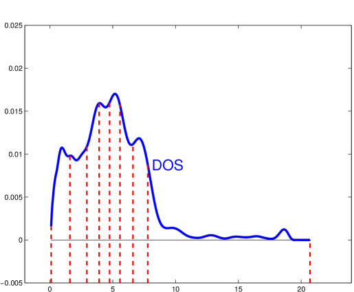
Another, somewhat related, use of density of states is in helping deploy spectrum slicing strategies [16, 18, 37]. The goal of such strategies is to subdivide a given interval of the spectrum into subintervals in order to compute the eigenvalues in each subinterval independently. Note that this is often done to balance memory usage rather than computational load. Indeed, load balancing cannot be assured by just having slices with roughly equal numbers of eigenvalues. With the availability of the spectral density function ϕitalic-ϕ\phi, slicing the spectrum contained in an interval [a,b]𝑎𝑏[a,\ b] into nssubscript𝑛𝑠n_{s} subintervals can be easily accomplished. Indeed, it suffices to find intervals [ti,ti+1]subscript𝑡𝑖subscript𝑡𝑖1[t_{i},\ t_{i+1}], i=0,,ns1𝑖0subscript𝑛𝑠1i=0,\cdots,n_{s}-1, with t0=asubscript𝑡0𝑎t_{0}=a and tns=bsubscript𝑡subscript𝑛𝑠𝑏t_{n_{s}}=b such that

titi+1ϕ(t)𝑑t=1nsabϕ(t)𝑑t,i=0,1,,ns1.formulae-sequencesuperscriptsubscriptsubscript𝑡𝑖subscript𝑡𝑖1italic-ϕ𝑡differential-d𝑡1subscript𝑛𝑠superscriptsubscript𝑎𝑏italic-ϕ𝑡differential-d𝑡𝑖01subscript𝑛𝑠1\int_{t_{i}}^{t_{i+1}}\phi(t)dt=\frac{1}{n_{s}}\int_{a}^{b}\phi(t)dt,\quad i=0,1,\cdots,n_{s}-1.

See Fig. 1 for an illustration and Section 5.3 for more details.
Refer to caption

Fig. 1: An illustration of slicing a spectrum into 888 subintervals [ti,ti+1]subscript𝑡𝑖subscript𝑡𝑖1[t_{i},\ t_{i+1}] (i=0,,7)𝑖07(i=0,\ldots,7). The solid blue curve represents a smoothed density of states (DOS) and the dotted red lines separate the subintervals.

A non-standard and important use of spectral densities is when estimating numerical ranks of matrices [32, 33]. In many applications, a given m×n𝑚𝑛m\times n data matrix A𝐴A (say with m>n𝑚𝑛m\!>\!n) is known to correspond to a phenomenon that should yield vectors lying in a low-dimensional space. With noise and approximations the resulting data is no longer of low-rank but it may be nearly low-rank in that its numerical rank is small. It may be important in these applications to obtain this numerical rank. In [32, 33] the authors developed a few heuristics that exploit the spectral density for this task. The main idea is that for a nearly low-rank matrix, the spectral density should be quite high near the origin of the matrix ATAsuperscript𝐴𝑇𝐴A^{T}A and it should drop quickly before increasing again. The numerical rank corresponds to the point when ϕitalic-ϕ\phi starts increasing again, i.e., when the derivative of the DOS changes signs. This simple strategy provides an efficient way to estimate the rank.

A straightforward way to obtain the spectral density of a given matrix A𝐴A is to compute all its eigenvalues but this approach is expensive for large matrices. Effective alternatives based on stochastic arguments have been developed, see, [20] for a survey. Essentially all the methods described in the literature to compute the DOS rely on performing a number of products of the matrix A𝐴A with random vectors. For sparse matrices or dense structured matrices with almost linear complexity matrix-vector products [4, 13], these products are inexpensive and so a fairly good approximation of the DOS can be obtained at a very low cost. On the other hand, not much work has been done to address the same problem for generalized eigenvalue problems

Ax=λBx.𝐴𝑥𝜆𝐵𝑥Ax=\lambda Bx. (3)

This paper focuses on this specific issue as well as on the related problem on implementing spectrum slicing techniques [18, 24]. From a theoretical viewpoint the problem may appear to be a trivial extension of the standard case. However, from a practical viewpoint several difficulties emerge, e.g., it is now necessary to solve a linear system with B𝐵B (or A𝐴A) each time we operate on vectors in the stochastic sampling procedure or in a Lanczos procedure. For large-scale problems discretized from 3D models, factorizing B𝐵B (or A𝐴A) tends to be prohibitively expensive and so this naturally leads to the question: Is it possible to completely avoid factorizations when computing the density of states for (3)? As will be seen the answer is yes, i.e., it is possible to get the DOS accurately without any factorizations and at a cost that is comparable with that of standard problems in many applications. For example, the matrix B𝐵B is often the mass matrix in discretizations such as the Finite Element Method (FEM). An important observation that is often made regarding these matrices is that they are strongly diagonally dominant.

In the remainder of the paper we will assume that A𝐴A and B𝐵B are Hermitian while, in addition, B𝐵B is positive definite. We will call λjsubscript𝜆𝑗\lambda_{j}, j=1,2,,n𝑗12𝑛j=1,2,\cdots,n the eigenvalues of the pencil (A,B)𝐴𝐵(A,B), and assume that they are labeled increasingly. We also denote by ujsubscript𝑢𝑗u_{j} the eigenvector corresponding to λjsubscript𝜆𝑗\lambda_{j}, so if U=[u1,u2,,un]𝑈subscript𝑢1subscript𝑢2subscript𝑢𝑛U=[u_{1},u_{2},\cdots,u_{n}] and Λ=diag(λ1,λ2,,λn)Λdiagsubscript𝜆1subscript𝜆2subscript𝜆𝑛\Lambda=\mbox{diag}(\lambda_{1},\lambda_{2},\cdots,\lambda_{n}), then the pencil (A,B)𝐴𝐵(A,B) admits the eigen-decomposition

UTAUsuperscript𝑈𝑇𝐴𝑈\displaystyle U^{T}AU =ΛabsentΛ\displaystyle=\Lambda (4)
UTBUsuperscript𝑈𝑇𝐵𝑈\displaystyle U^{T}BU =I.absent𝐼\displaystyle=I\ . (5)

The rest of the paper is organized as follows. Section 2 discusses a few techniques to avoid direct factorizations when extending standard approaches for computing the DOS to the generalized eigenvalue problem. Section 3 presents the extension of the classical Kernel Polynomial Method (KPM) and Section 4 studies the Lanczos method from the angle of quadrature. We provide some numerical examples in Section 5 and draw some concluding remarks in Section 6.

2 Symmetrizing the generalized eigenvalue problem

A common way to express the generalized eigenvalue problem (3) is to multiply through by B1superscript𝐵1B^{-1}:

B1Ax=λx.superscript𝐵1𝐴𝑥𝜆𝑥B^{-1}Ax=\lambda x. (6)

This is now in the standard form but the matrix involved is non-Hermitian. However, as is well-known, the matrix B1Asuperscript𝐵1𝐴B^{-1}A is self-adjoint with respect to the B𝐵B-inner product and this observation allows one to use standard methods, such as the Lanczos algorithm, that are designed for Hermitian matrices.

Another way to extend standard approaches for computing the spectral density is to transform the problem (3) into a standard one via the Cholesky factorization. First, assume that the Cholesky factorization of B𝐵B is available and let it be written as B=LL𝖳𝐵𝐿superscript𝐿𝖳B=LL^{\mathsf{T}}. Then the original problem (3) can also be rewritten as

L1AL𝖳y=λy,withy=L𝖳x,formulae-sequencesuperscript𝐿1𝐴superscript𝐿𝖳𝑦𝜆𝑦with𝑦superscript𝐿𝖳𝑥L^{-1}AL^{-\mathsf{T}}y=\lambda y,\quad\mbox{with}\quad y=L^{\mathsf{T}}x, (7)

which takes the standard form with a Hermitian coefficient matrix. This allows us to express the density of states from that of a standard problem. This straightforward solution faces a number of issues. Foremost among these is the fact that the Cholesky factorization may not be available or that it may be too expensive to compute. In the case of FEM methods, the factorization of B𝐵B may be too costly for 3D3𝐷3D problems.

Note that the matrix square root factorization can also be used in the same way. Here the original problem (3) is transformed into the equivalent problem:

B1/2AB1/2y=λy,withy=B1/2x,formulae-sequencesuperscript𝐵12𝐴superscript𝐵12𝑦𝜆𝑦with𝑦superscript𝐵12𝑥B^{-1/2}AB^{-1/2}y=\lambda y,\quad\mbox{with}\quad y=B^{1/2}x, (8)

which also assumes the standard form with a Hermitian coefficient matrix. The square root factorization is usually expensive to compute and may appear to be impractical at first. However, in the common situation mentioned above where B𝐵B is strongly diagonally dominant, the action of B1/2superscript𝐵12B^{-1/2} as well B1superscript𝐵1B^{-1} on a vector can be easily approximated by the matrix-vector product associated with a low degree polynomial in B𝐵B. This is discussed next.

2.1 Approximating actions of B1superscript𝐵1B^{-1} and B1/2superscript𝐵12B^{-1/2} on vectors

As was seen above computing the DOS for a pair of matrices requires matrix-vector products with either B1Asuperscript𝐵1𝐴B^{-1}A, or L1AL𝖳superscript𝐿1𝐴superscript𝐿𝖳L^{-1}AL^{-\mathsf{T}} or with B1/2AB1/2superscript𝐵12𝐴superscript𝐵12B^{-1/2}AB^{-1/2}. Methods based on the first two cases can be implemented with direct methods but this requires a factorization of B𝐵B. Computing the Cholesky, or any other factorization of B𝐵B is not always economically feasible for large problems. It is therefore important to explore alternatives based on the third case in which polynomial approximations of B1/2superscript𝐵12B^{-1/2} are exploited.

All we need to apply the methods described in this paper is a way to compute B1/2vsuperscript𝐵12𝑣B^{-1/2}v or B1vsuperscript𝐵1𝑣B^{-1}v for an arbitrary vector v𝑣v. These calculations amount to evaluating f(B)v𝑓𝐵𝑣f(B)v where f(λ)=λ1/2𝑓𝜆superscript𝜆12f(\lambda)=\lambda^{-1/2} in one case and f(λ)=1/λ𝑓𝜆1𝜆f(\lambda)=1/\lambda in the other. Essentially the same method is used in both cases, in that f(B)v𝑓𝐵𝑣f(B)v is replaced by fk(B)vsubscript𝑓𝑘𝐵𝑣f_{k}(B)v where fksubscript𝑓𝑘f_{k} is an order k𝑘k polynomial approximation to the function f𝑓f obtained by a least-squares approach. Computing B1/2vsuperscript𝐵12𝑣B^{-1/2}v, is a problem that was examined at length in the literature – see for example [2, 5, 14] and references therein. Here we use a simple scheme that relies on a Chebyshev approximation of the square root function in the interval [a,b]𝑎𝑏[a,\ b] where a>0𝑎0a\!>\!0.

Recall that any function that is analytic in [a,b]𝑎𝑏[a,\ b] can be expanded in Chebyshev polynomials. To do so, the first step is to map [a,b]𝑎𝑏[a,\ b] into the interval [1, 1]11[-1,\ 1], i.e., we impose the change of variables from λ[a,b]𝜆𝑎𝑏\lambda\!\in\![a,\ b] to t[1, 1]𝑡11t\!\in\![-1,\ 1]:

t=λchwithc=a+b2,h=ba2.formulae-sequence𝑡𝜆𝑐withformulae-sequence𝑐𝑎𝑏2𝑏𝑎2t=\frac{\lambda-c}{h}\quad\mbox{with}\quad c=\frac{a+b}{2},\quad h=\frac{b-a}{2}\ .

In this way the function is transformed into a function f𝑓f with variables in the interval [1, 1]11[-1,\ 1]. It is this f𝑓f that is approximated using the truncated Chebyshev expansion:

fk(t)=i=0kγiTi(t)withγi=2δi0π11f(s)Ti(s)1s2𝑑s,formulae-sequencesubscript𝑓𝑘𝑡superscriptsubscript𝑖0𝑘subscript𝛾𝑖subscript𝑇𝑖𝑡withsubscript𝛾𝑖2subscript𝛿𝑖0𝜋superscriptsubscript11𝑓𝑠subscript𝑇𝑖𝑠1superscript𝑠2differential-d𝑠f_{k}(t)=\sum_{i=0}^{k}\gamma_{i}T_{i}(t)\quad\text{with}\quad\gamma_{i}=\frac{2-\delta_{i0}}{\pi}\int_{-1}^{1}\frac{f(s)T_{i}(s)}{\sqrt{1-s^{2}}}ds, (9)

where Ti(s)subscript𝑇𝑖𝑠T_{i}(s) is the Chebyshev polynomial of the first kind of degree i𝑖i. Here δijsubscript𝛿𝑖𝑗\delta_{ij} is the Kronecker δ𝛿\delta symbol so that 2δk02subscript𝛿𝑘02-\delta_{k0} is equal to 1 when k=0𝑘0k=0 and to 2 otherwise.

Recall that Tisubscript𝑇𝑖T_{i}’s are orthogonal with respect to the inner product

p,q=11p(s)q(s)1s2𝑑s.𝑝𝑞superscriptsubscript11𝑝𝑠𝑞𝑠1superscript𝑠2differential-d𝑠\left\langle p,q\right\rangle=\int_{-1}^{1}\frac{p(s)q(s)}{\sqrt{1-s^{2}}}ds. (10)

We denote by .\|.\|_{\infty} the supremum norm and by .C\|.\|_{C} the L2subscript𝐿2L_{2} norm associated with the above dot product:

pC=[11p(s)21s2𝑑s]1/2.subscriptnorm𝑝𝐶superscriptdelimited-[]superscriptsubscript11𝑝superscript𝑠21superscript𝑠2differential-d𝑠12\|p\|_{C}=\left[\int_{-1}^{1}\frac{p(s)^{2}}{\sqrt{1-s^{2}}}ds\right]^{1/2}. (11)

Note in passing that Tisubscript𝑇𝑖T_{i}’s do not have a unit norm with respect to (11) but that the following normalized sequence is orthonormal:

T^i(s)=2δi0πTi(s),subscript^𝑇𝑖𝑠2subscript𝛿𝑖0𝜋subscript𝑇𝑖𝑠\hat{T}_{i}(s)=\sqrt{\frac{2-\delta_{i0}}{\pi}}T_{i}(s), (12)

so that (9) can be rewritten as fk(t)=i=0kγ^iT^i(t)subscript𝑓𝑘𝑡superscriptsubscript𝑖0𝑘subscript^𝛾𝑖subscript^𝑇𝑖𝑡f_{k}(t)=\sum_{i=0}^{k}\hat{\gamma}_{i}\hat{T}_{i}(t) with γ^i=f(t),T^i(t)subscript^𝛾𝑖𝑓𝑡subscript^𝑇𝑖𝑡\hat{\gamma}_{i}=\langle f(t),\hat{T}_{i}(t)\rangle.

The integrals in (9) are computed using Gauss-Chebychev quadrature. The accuracy of the approximation and therefore the degree needed to obtain a suitable approximation to use in replacement of f(B)v𝑓𝐵𝑣f(B)v depends essentially on the degree of smoothness of f𝑓f. One issue here is to determine the number of integration points to use. Recall that when we use Gauss-Chebyshev quadrature with ν𝜈\nu points, the calculated integral is exact for all polynomials of degree 2ν1absent2𝜈1\leq 2\nu-1.

The reasoning for selecting ν𝜈\nu is as follows. Let pKsubscript𝑝𝐾p_{K} be the truncated Chebyshev expansion of f𝑓f, with Kkmuch-greater-than𝐾𝑘K\gg k. Then for ik𝑖𝑘i\leq k the coefficients γ^isubscript^𝛾𝑖\hat{\gamma}_{i} for ik𝑖𝑘i\leq k are the same for pksubscript𝑝𝑘p_{k} and for pKsubscript𝑝𝐾p_{K} and they are:

γ^i=f,T^i=fpK,T^i+pK,T^i=pK,T^i.subscript^𝛾𝑖𝑓subscript^𝑇𝑖𝑓subscript𝑝𝐾subscript^𝑇𝑖subscript𝑝𝐾subscript^𝑇𝑖subscript𝑝𝐾subscript^𝑇𝑖\hat{\gamma}_{i}=\left\langle f,\hat{T}_{i}\right\rangle=\left\langle f-p_{K},\hat{T}_{i}\right\rangle+\left\langle p_{K},\hat{T}_{i}\right\rangle=\left\langle p_{K},\hat{T}_{i}\right\rangle.

The last equality is due to the orthogonality of the error to the Tisubscript𝑇𝑖T_{i}’s, when iK𝑖𝐾i\leq K. Now observe that since pK(t)T^i(t)subscript𝑝𝐾𝑡subscript^𝑇𝑖𝑡p_{K}(t)\hat{T}_{i}(t) is a polynomial of degree K+kabsent𝐾𝑘\leq K+k the integral pK,T^isubscript𝑝𝐾subscript^𝑇𝑖\langle p_{K},\hat{T}_{i}\rangle will be computed exactly by the Gauss-Chebyshev rule as long as K+k2ν1𝐾𝑘2𝜈1K+k\leq 2\nu-1, i.e., for ν(K+k+1)/2𝜈𝐾𝑘12\nu\geq(K+k+1)/2. For example, when K=2k𝐾2𝑘K=2k then for ν(3k+1)/2𝜈3𝑘12\nu\geq(3k+1)/2, γ^isubscript^𝛾𝑖\hat{\gamma}_{i} will be the exact coefficient not for f(t)𝑓𝑡f(t), but for p2ksubscript𝑝2𝑘p_{2k} the degree 2k2𝑘2k Chebyshev expansion which is usually much closer to f𝑓f than pksubscript𝑝𝑘p_{k}. While ν=(3k+1)/2𝜈3𝑘12\nu=\lceil(3k+1)/2\rceil is usually sufficient, we prefer a lower margin for error and select ν=4k𝜈4𝑘\nu=4k bearing in mind that the cost of quadrature is negligible.

2.2 Analysis of the approximation accuracy

Consider the two functions f1(λ)=λ1/2subscript𝑓1𝜆superscript𝜆12f_{1}(\lambda)=\lambda^{-1/2} and f2(λ)=λ1subscript𝑓2𝜆superscript𝜆1f_{2}(\lambda)=\lambda^{-1} over λ[a,b]𝜆𝑎𝑏\lambda\!\in\![a,\ b] where a>0𝑎0a\!>\!0. It is assumed that the interval [a,b]𝑎𝑏[a,\ b] contains the spectrum of B𝐵B - with ideally a=λmin(B)𝑎subscript𝜆𝑚𝑖𝑛𝐵a=\lambda_{min}(B), b=λmax(B)𝑏subscript𝜆𝑚𝑎𝑥𝐵b=\lambda_{max}(B). We set c=(a+b)/2𝑐𝑎𝑏2c=(a+b)/2, h=(ba)/2𝑏𝑎2h=(b-a)/2. As mentioned above we need to transform the interval [a,b]𝑎𝑏[a,\ b] into [1, 1]11[-1,\ 1], so the transformed functions being approximated are in fact

g(t)𝑔𝑡\displaystyle g(t) =(c+ht)1/2,absentsuperscript𝑐𝑡12\displaystyle=(c+ht)^{-1/2}, (13)
q(t)𝑞𝑡\displaystyle q(t) =(c+ht)1,absentsuperscript𝑐𝑡1\displaystyle=(c+ht)^{-1}, (14)

with the variable t𝑡t now in [1, 1]11[-1,\ 1]. These two functions are clearly analytic in the interval [1, 1]11[-1,\ 1] and they have a singularity when c+ht=0𝑐𝑡0c+ht=0, i.e., at ts=c/hsubscript𝑡𝑠𝑐t_{s}=-c/h which is less than 11-1. Existing results in the literature will help analyze the convergence of the truncated Chebyshev expansion in situations such as these, see, e.g., [31].

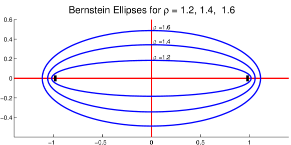
We can apply the result of Theorem 8.2 in the book [31] to show a strong convergence result. The Joukowsky transform (z+1/z)/2𝑧1𝑧2(z+1/z)/2 maps the circle C(0,ρ)𝐶0𝜌C(0,\rho) into an ellipse Eρsubscript𝐸𝜌E_{\rho}, with major semi-axis (ρ+ρ1)/2𝜌superscript𝜌12(\rho+\rho^{-1})/2 and focii 1,111-1,1. There are two values of ρ𝜌\rho that give the same ellipse and they are inverses of each other. We assume that ρ>1𝜌1\rho\!>\!1. The ellipse Eρsubscript𝐸𝜌E_{\rho} is called the Bernstein ellipse in the framework of the theorem in [31] which is restated below for the present context. See Fig. 2 for an illustration of Bernstein ellipses corresponding to different ρ𝜌\rho’s.

Theorem 1.

[31, Theorem 8.2] Let a function f𝑓f analytic in [1, 1]11[-1,\ 1] be analytically continuable to the open Bernstein ellipse Eρsubscript𝐸𝜌E_{\rho} where it satisfies |f(t)|M(ρ)𝑓𝑡𝑀𝜌|f(t)|\leq M(\rho) for some M(ρ)𝑀𝜌M(\rho). Then for each k0𝑘0k\geq 0, its truncated Chebyshev expansion fksubscript𝑓𝑘f_{k} (eq. (9)) satisfies:

ffk2M(ρ)ρkρ1.subscriptnorm𝑓subscript𝑓𝑘2𝑀𝜌superscript𝜌𝑘𝜌1\|f-f_{k}\|_{\infty}\leq\frac{2M(\rho)\rho^{-k}}{\rho-1}. (15)

Refer to caption

Fig. 2: Bernstein ellipses for ρ=1.2,1.4,1.6𝜌1.21.41.6\rho=1.2,1.4,1.6.

The Bernstein ellipse should not contain the point of singularity. Therefore, for the two functions under consideration, we should take any ρ>1𝜌1\rho>1 such that (ρ+ρ1)/2<c/h𝜌superscript𝜌12𝑐(\rho+\rho^{-1})/2\!<\!c/h, i.e., ρ𝜌\rho must satisfy:

1<ρ<ch+(ch)21.1𝜌𝑐superscript𝑐211<\rho<\frac{c}{h}+\sqrt{\left(\frac{c}{h}\right)^{2}-1}. (16)

The next ingredient from the theorem is an upper bound M(ρ)𝑀𝜌M(\rho) for |f(t)|𝑓𝑡|f(t)| in Eρsubscript𝐸𝜌E_{\rho}. In fact the maximum value of this modulus is computable for both functions under consideration and it is given in the next lemma.

Lemma 2.

Let ρ𝜌\rho be given such that (16) is satisfied. Then the maximum modulii of the functions (13) and (14) for tEρ𝑡subscript𝐸𝜌t\!\in\!E_{\rho} are given, respectively, by

Mg(ρ)subscript𝑀𝑔𝜌\displaystyle M_{g}(\rho) =1chρ+ρ12,absent1𝑐𝜌superscript𝜌12\displaystyle=\frac{1}{\sqrt{c-h\frac{\rho+\rho^{-1}}{2}}}, (17)
Mq(ρ)subscript𝑀𝑞𝜌\displaystyle M_{q}(\rho) =1chρ+ρ12.absent1𝑐𝜌superscript𝜌12\displaystyle=\frac{1}{c-h\frac{\rho+\rho^{-1}}{2}}. (18)
Proof.

Denote d=c+ht𝑑𝑐𝑡d=c+ht the term inside the parentheses of (13) and (14) and write tEρ𝑡subscript𝐸𝜌t\!\in\!E_{\rho} as: t=12[ρeiθ+ρ1eiθ]𝑡12delimited-[]𝜌superscript𝑒𝑖𝜃superscript𝜌1superscript𝑒𝑖𝜃t={1\over 2}[\rho e^{i\theta}+\rho^{-1}e^{-i\theta}]. Then d=c+h(ρeiθ+ρ1eiθ)/2𝑑𝑐𝜌superscript𝑒𝑖𝜃superscript𝜌1superscript𝑒𝑖𝜃2d=c+h(\rho e^{i\theta}+\rho^{-1}e^{-i\theta})/2 and

|d|2superscript𝑑2\displaystyle|d|^{2} =(c+ht)(c+ht¯)=c2+hc(t+t¯)+h2tt¯absent𝑐𝑡𝑐¯𝑡superscript𝑐2𝑐𝑡¯𝑡superscript2𝑡¯𝑡\displaystyle=(c+ht)(c+h\bar{t})=c^{2}+hc(t+\bar{t})+h^{2}t\bar{t}
=c2+hc(ρ+ρ1)cosθ+h24[ρ2+ρ2+2cos(2θ)].absentsuperscript𝑐2𝑐𝜌superscript𝜌1𝜃superscript24delimited-[]superscript𝜌2superscript𝜌222𝜃\displaystyle=c^{2}+hc(\rho+\rho^{-1})\cos\theta+\frac{h^{2}}{4}[\rho^{2}+\rho^{-2}+2\cos(2\theta)].

Observe that ρ2+ρ2=(ρ+ρ1)22superscript𝜌2superscript𝜌2superscript𝜌superscript𝜌122\rho^{2}+\rho^{-2}=(\rho+\rho^{-1})^{2}-2 and cos(2θ)=2cos2θ12𝜃2superscript2𝜃1\cos(2\theta)=2\cos^{2}\theta-1. Therefore,

|d|2superscript𝑑2\displaystyle|d|^{2} =c2+hc(ρ+ρ1)cosθ+h24[(ρ+ρ1)22(1cos(2θ))]absentsuperscript𝑐2𝑐𝜌superscript𝜌1𝜃superscript24delimited-[]superscript𝜌superscript𝜌12212𝜃\displaystyle=c^{2}+hc(\rho+\rho^{-1})\cos\theta+\frac{h^{2}}{4}[(\rho+\rho^{-1})^{2}-2(1-\cos(2\theta))]
=c2+hc(ρ+ρ1)cosθ+h24[(ρ+ρ1)24(1cos2θ)]absentsuperscript𝑐2𝑐𝜌superscript𝜌1𝜃superscript24delimited-[]superscript𝜌superscript𝜌1241superscript2𝜃\displaystyle=c^{2}+hc(\rho+\rho^{-1})\cos\theta+\frac{h^{2}}{4}[(\rho+\rho^{-1})^{2}-4(1-\cos^{2}\theta)]
=[c+hρ+ρ12cosθ]2+h24[(ρ+ρ1)24](1cos2θ)absentsuperscriptdelimited-[]𝑐𝜌superscript𝜌12𝜃2superscript24delimited-[]superscript𝜌superscript𝜌1241superscript2𝜃\displaystyle=\left[c+h\frac{\rho+\rho^{-1}}{2}\cos\theta\right]^{2}+\frac{h^{2}}{4}\left[(\rho+\rho^{-1})^{2}-4\right](1-\cos^{2}\theta)
=[c+hρ+ρ12cosθ]2+h2[(ρ+ρ12)21]sin2θ.absentsuperscriptdelimited-[]𝑐𝜌superscript𝜌12𝜃2superscript2delimited-[]superscript𝜌superscript𝜌1221superscript2𝜃\displaystyle=\left[c+h\frac{\rho+\rho^{-1}}{2}\cos\theta\right]^{2}+h^{2}\left[\left(\frac{\rho+\rho^{-1}}{2}\right)^{2}-1\right]\sin^{2}\theta.

Since (ρ+ρ1)/2>1𝜌superscript𝜌121(\rho+\rho^{-1})/2\!>\!1, the second term in brackets is positive and it is then clear that the minimum value of |d|2superscript𝑑2|d|^{2} is reached when θ=π𝜃𝜋\theta=\pi and the corresponding |d|𝑑|d| is ch(ρ+ρ1)/2𝑐𝜌superscript𝜌12c-h(\rho+\rho^{-1})/2. Inverting this gives (18). Taking the inverse square root yields (17) and this completes the proof. ∎

Note that, as expected, both maxima go to infinity as ρ𝜌\rho approaches its right (upper) bound given by (16). We can now state the following theorem which simply applies Theorem 1 to the functions (13) and (14), using the bounds for M(ρ)𝑀𝜌M(\rho) obtained in Lemma 2.

Theorem 3.

Let g𝑔g and q𝑞q be the functions given by (13) and (14) and let ρ𝜌\rho be any real number that satisfies the inequalities (16). Then the truncated Chebyshev expansions gk1subscript𝑔subscript𝑘1g_{k_{1}} and qk2subscript𝑞subscript𝑘2q_{k_{2}} of g𝑔g and q𝑞q, respectively, satisfy:

ggk1subscriptnorm𝑔subscript𝑔subscript𝑘1\displaystyle\|g-g_{k_{1}}\|_{\infty} 2ρk1(ρ1)chρ+ρ12,absent2superscript𝜌subscript𝑘1𝜌1𝑐𝜌superscript𝜌12\displaystyle\leq\frac{2\rho^{-k_{1}}}{(\rho-1)\sqrt{c-h\frac{\rho+\rho^{-1}}{2}}}, (19)
qqk2subscriptnorm𝑞subscript𝑞subscript𝑘2\displaystyle\|q-q_{k_{2}}\|_{\infty} 2ρk2(ρ1)(chρ+ρ12).absent2superscript𝜌subscript𝑘2𝜌1𝑐𝜌superscript𝜌12\displaystyle\leq\frac{2\rho^{-k_{2}}}{(\rho-1)\left(c-h\frac{\rho+\rho^{-1}}{2}\right)}. (20)

Theorem 8.1 in [31], upon which Theorem 1 is based, states that the coefficients γisubscript𝛾𝑖\gamma_{i} in (9) decay geometrically, i.e.,

|γk|2M(ρ)ρk.subscript𝛾𝑘2𝑀𝜌superscript𝜌𝑘|\gamma_{k}|\leq 2M(\rho)\rho^{-k}. (21)

Based on the above inequality, it is now possible to establish the following result for the approximation error of gk1subscript𝑔subscript𝑘1g_{k_{1}} and qk2subscript𝑞subscript𝑘2q_{k_{2}} measured in the Chebyshev norm.

Proposition 4.

Under the same assumptions as for Theorem 3, the truncated Chebyshev expansions gk1subscript𝑔subscript𝑘1g_{k_{1}} and qk2subscript𝑞subscript𝑘2q_{k_{2}} of g𝑔g and q𝑞q, satisfy, respectively:

ggk1Csubscriptnorm𝑔subscript𝑔subscript𝑘1𝐶\displaystyle\|g-g_{k_{1}}\|_{C} 2πρ21ρk1chρ+ρ12,absent2𝜋superscript𝜌21superscript𝜌subscript𝑘1𝑐𝜌superscript𝜌12\displaystyle\leq\sqrt{\frac{2\pi}{\rho^{2}-1}}\frac{\rho^{-{k_{1}}}}{\sqrt{c-h\frac{\rho+\rho^{-1}}{2}}}, (22)
qqk2Csubscriptnorm𝑞subscript𝑞subscript𝑘2𝐶\displaystyle\|q-q_{k_{2}}\|_{C} 2πρ21ρk2(chρ+ρ12).absent2𝜋superscript𝜌21superscript𝜌subscript𝑘2𝑐𝜌superscript𝜌12\displaystyle\leq\sqrt{\frac{2\pi}{\rho^{2}-1}}\frac{\rho^{-k_{2}}}{\left(c-h\frac{\rho+\rho^{-1}}{2}\right)}. (23)
Proof.

For any function f𝑓f expandable as in (9), we have

f(t)fk(t)=i=k+1γiTi(t).𝑓𝑡subscript𝑓𝑘𝑡superscriptsubscript𝑖𝑘1subscript𝛾𝑖subscript𝑇𝑖𝑡f(t)-f_{k}(t)=\sum_{i=k+1}^{\infty}\gamma_{i}T_{i}(t).

Because of the orthogonality of the Chebyshev polynomials and the inequality (21), we obtain

f(t)fk(t)C2superscriptsubscriptnorm𝑓𝑡subscript𝑓𝑘𝑡𝐶2\displaystyle\|f(t)-f_{k}(t)\|_{C}^{2} =i=k+1|γi|2Ti(t)C2i=k+14M(ρ)2ρ2iπ2absentsuperscriptsubscript𝑖𝑘1superscriptsubscript𝛾𝑖2superscriptsubscriptnormsubscript𝑇𝑖𝑡𝐶2superscriptsubscript𝑖𝑘14𝑀superscript𝜌2superscript𝜌2𝑖𝜋2\displaystyle=\sum_{i=k+1}^{\infty}|\gamma_{i}|^{2}\|T_{i}(t)\|_{C}^{2}\leq\sum_{i=k+1}^{\infty}4M(\rho)^{2}\rho^{-2i}\frac{\pi}{2}
2M(ρ)2πρ2(k+1)11ρ2=2M(ρ)2πρ2k1ρ21.absent2𝑀superscript𝜌2𝜋superscript𝜌2𝑘111superscript𝜌22𝑀superscript𝜌2𝜋superscript𝜌2𝑘1superscript𝜌21\displaystyle\leq 2M(\rho)^{2}\pi\rho^{-2(k+1)}\frac{1}{1-\rho^{-2}}=2M(\rho)^{2}\pi\rho^{-2k}\frac{1}{\rho^{2}-1}.

Taking the square root and replacing the values of M(ρ)𝑀𝜌M(\rho) from Lemma 2 yield the two inequalities. ∎

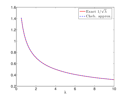
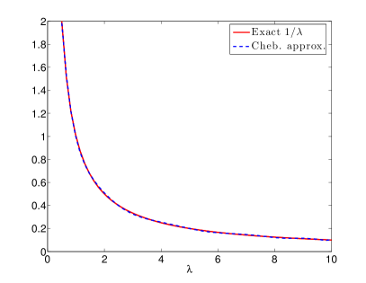
Both Theorem 3 and Proposition 4 show that the Chebyshev expansions gk1subscript𝑔subscript𝑘1g_{k_{1}} and qk2subscript𝑞subscript𝑘2q_{k_{2}} converge geometrically. The plot in Fig. 3 indicates that a low degree is sufficient to reach a reasonable accuracy for the needs of computing the DOS.
Refer to caption
Refer to caption
Fig. 3: Degree 101010 Chebyshev polynomial approximations to 1/λ1𝜆1/\sqrt{\lambda} and 1/λ1𝜆1/\lambda on the interval [0.5, 10]0.510[0.5,\ 10].

2.3 Bounds involving the condition number of B𝐵B

Theorem 3 shows that the asymptotic convergence rate increases with ρ𝜌\rho. However, the “optimal” value of ρ𝜌\rho, i.e., the one that yields the smallest bounds in (19) or (20), depends on kisubscript𝑘𝑖k_{i} and is hard to choose in practice. Here, we will discuss two simple choices for ρ𝜌\rho that will help analyze the convergence. First, we select ρ=ρ0c/h𝜌subscript𝜌0𝑐\rho=\rho_{0}\equiv c/h which satisfies the bounds (16). It leads to

Mg(ρ0)=2ch2/c,Mq(ρ0)=(Mg(ρ0))2.formulae-sequencesubscript𝑀𝑔subscript𝜌02𝑐superscript2𝑐subscript𝑀𝑞subscript𝜌0superscriptsubscript𝑀𝑔subscript𝜌02M_{g}(\rho_{0})=\frac{\sqrt{2}}{\sqrt{c-h^{2}/c}},\qquad M_{q}(\rho_{0})=(M_{g}(\rho_{0}))^{2}\ . (24)

Note that in the context of our problem, if we denote by λmax(B),λmin(B)subscript𝜆𝑚𝑎𝑥𝐵subscript𝜆𝑚𝑖𝑛𝐵\lambda_{max}(B),\lambda_{min}(B) the largest and smallest eigenvalues of B𝐵B and by κ𝜅\kappa its spectral condition number, then

ρ0=c/h=λmax(B)+λmin(B)λmax(B)λmin(B)=κ+1κ1,subscript𝜌0𝑐subscript𝜆𝑚𝑎𝑥𝐵subscript𝜆𝑚𝑖𝑛𝐵subscript𝜆𝑚𝑎𝑥𝐵subscript𝜆𝑚𝑖𝑛𝐵𝜅1𝜅1\rho_{0}=c/h=\frac{\lambda_{max}(B)+\lambda_{min}(B)}{\lambda_{max}(B)-\lambda_{min}(B)}=\frac{\kappa+1}{\kappa-1},

and therefore, for this choice of ρ𝜌\rho, the bounds of the theorem evolve asymptotically like (κ1κ+1)ksuperscript𝜅1𝜅1𝑘(\frac{\kappa-1}{\kappa+1})^{k}. A slightly more elaborate selection of ρ𝜌\rho is the value for which (ρ+ρ1)/2=c/h𝜌superscript𝜌12𝑐(\rho+\rho^{-1})/2=\sqrt{c/h} which is ρ1=c/h+(c/h)1subscript𝜌1𝑐𝑐1\rho_{1}=\sqrt{c/h}+\sqrt{(c/h)-1}. For t1𝑡1t\geq 1,  t+t21𝑡superscript𝑡21t+\sqrt{t^{2}-1} is an increasing function and therefore, 1ρ1(c/h)+(c/h)211subscript𝜌1𝑐superscript𝑐211\leq\rho_{1}\leq(c/h)+\sqrt{(c/h)^{2}-1} and so the bounds (16) are satisfied. With this we get:

Mg(ρ1)=1chc,Mq(ρ1)=(Mg(ρ1))2.formulae-sequencesubscript𝑀𝑔subscript𝜌11𝑐𝑐subscript𝑀𝑞subscript𝜌1superscriptsubscript𝑀𝑔subscript𝜌12M_{g}(\rho_{1})=\frac{1}{\sqrt{c-\sqrt{hc}}},\qquad M_{q}(\rho_{1})=(M_{g}(\rho_{1}))^{2}\ .

In addition, we note that ρ1subscript𝜌1\rho_{1} can also be expressed in terms of the spectral condition number κ𝜅\kappa of B𝐵B as follows: ρ1=[κ+1+2]/[κ1]subscript𝜌1delimited-[]𝜅12delimited-[]𝜅1\rho_{1}=[\sqrt{\kappa+1}+\sqrt{2}]/[\sqrt{\kappa-1}]. The resulting term ρ1ksuperscriptsubscript𝜌1𝑘\rho_{1}^{-k} in (19) and (20) will decay much faster than ρ0ksuperscriptsubscript𝜌0𝑘\rho_{0}^{-k} when κ𝜅\kappa is larger than 222. Both choices of ρ𝜌\rho show that for a fixed degree k𝑘k, a smaller κ𝜅\kappa will result in faster convergence.

If B𝐵B is a mass matrix obtained from a FEM discretization, κ𝜅\kappa can become very large for a general nonuniform mesh. One simple technique to reduce the value of κ𝜅\kappa is to use diagonal scaling [17, 35, 36]. Suppose D=diag(B)𝐷diag𝐵D=\operatorname{diag}(B), then by congruence, the following problem has the same eigenvalues as (3)

D1/2AD1/2z=λD1/2BD1/2z,withz=D1/2x.formulae-sequencesuperscript𝐷12𝐴superscript𝐷12𝑧𝜆superscript𝐷12𝐵superscript𝐷12𝑧with𝑧superscript𝐷12𝑥D^{-1/2}AD^{-1/2}z=\lambda D^{-1/2}BD^{-1/2}z,\quad\mbox{with}\quad z=D^{1/2}x. (25)

It was shown in [35, 36] that, for any conforming mesh of tetrahedral (P1) elements in three dimensions, κ(D1/2BD1/2)𝜅superscript𝐷12𝐵superscript𝐷12\kappa(D^{-1/2}BD^{-1/2}) is bounded by 555 and for a mesh of rectangular bi-linear (Q1) elements in two dimensions, κ(D1/2BD1/2)𝜅superscript𝐷12𝐵superscript𝐷12\kappa(D^{-1/2}BD^{-1/2}) is bounded by 999. Moreover, this diagonal scaling technique has also been exploited to reduce the spectral condition number of graph Laplacians in the network analysis [3]. As a result, we will always preprocess the matrix pencil (A,B)𝐴𝐵(A,B) by diagonal scaling before computing the DOS.

With the approximations in (9), we obtain

B1superscript𝐵1\displaystyle B^{-1} gk1(B):=i=0k1γiTi[(BcI)/h],absentsubscript𝑔subscript𝑘1𝐵assignsuperscriptsubscript𝑖0subscript𝑘1subscript𝛾𝑖subscript𝑇𝑖delimited-[]𝐵𝑐𝐼\displaystyle\approx g_{k_{1}}(B):=\sum_{i=0}^{k_{1}}\gamma_{i}T_{i}[(B-cI)/h], (26)
B1/2superscript𝐵12\displaystyle B^{-1/2} qk2(B):=i=0k2βiTi[(BcI)/h].absentsubscript𝑞subscript𝑘2𝐵assignsuperscriptsubscript𝑖0subscript𝑘2subscript𝛽𝑖subscript𝑇𝑖delimited-[]𝐵𝑐𝐼\displaystyle\approx q_{k_{2}}(B):=\sum_{i=0}^{k_{2}}\beta_{i}T_{i}[(B-cI)/h]. (27)

Using the above approximations to replace B1superscript𝐵1B^{-1} and B1/2superscript𝐵12B^{-1/2} in (6) and (8), will amount to computing the DOS of the modified problem

gk1(B)Ax~=λ~x~.subscript𝑔subscript𝑘1𝐵𝐴~𝑥~𝜆~𝑥g_{k_{1}}(B)A\tilde{x}=\tilde{\lambda}\tilde{x}. (28)

Therefore, it is important to show that the distance between λ~~𝜆\tilde{\lambda} and λ𝜆\lambda is small when gk1subscript𝑔subscript𝑘1g_{k_{1}} and qk2subscript𝑞subscript𝑘2q_{k_{2}} reach a certain accuracy. We will need the following perturbation result for Hermitian definite pencils.

Theorem 5.

[21, Theorem 2.2] Suppose that a Hermitian definite pencil (A,B)𝐴𝐵(A,B) has eigenvalues λ1λ2λnsubscript𝜆1subscript𝜆2subscript𝜆𝑛\lambda_{1}\leq\lambda_{2}\leq\dots\leq\lambda_{n}. If ΔA,ΔBΔ𝐴Δ𝐵\Delta A,\Delta B are Hermitian and ΔB2<λmin(B)subscriptnormΔ𝐵2subscript𝜆𝑚𝑖𝑛𝐵||\Delta B||_{2}<\lambda_{min}(B), then (A+ΔA,B+ΔB)𝐴Δ𝐴𝐵Δ𝐵(A+\Delta A,B+\Delta B) is a Hermitian definite pencil whose eigenvalues λ^1λ^2λ^nsubscript^𝜆1subscript^𝜆2subscript^𝜆𝑛\hat{\lambda}_{1}\leq\hat{\lambda}_{2}\leq\dots\leq\hat{\lambda}_{n} satisfy

|λiλ^i|ΔA2λmin(B)+|λi|λmin(B)+ΔA2λmin(B)(λmin(B)ΔB2)ΔB2.subscript𝜆𝑖subscript^𝜆𝑖subscriptnormΔ𝐴2subscript𝜆𝑚𝑖𝑛𝐵subscript𝜆𝑖subscript𝜆𝑚𝑖𝑛𝐵subscriptnormΔ𝐴2subscript𝜆𝑚𝑖𝑛𝐵subscript𝜆𝑚𝑖𝑛𝐵subscriptnormΔ𝐵2subscriptnormΔ𝐵2\displaystyle|\lambda_{i}-\hat{\lambda}_{i}|\leq\frac{||\Delta A||_{2}}{\lambda_{min}(B)}+\frac{|\lambda_{i}|\lambda_{min}(B)+||\Delta A||_{2}}{\lambda_{min}(B)(\lambda_{min}(B)-||\Delta B||_{2})}||\Delta B||_{2}. (29)

In the context of (28), the perturbation ΔBΔ𝐵\Delta B in Theorem 6 corresponds to the approximation error of gk1(B)subscript𝑔subscript𝑘1𝐵g_{k_{1}}(B) to B1superscript𝐵1B^{-1}. This implies that we can rewrite (28) in the form of

Ax~=λ~(B+ΔB)x~withΔB=(gk1(B))1B,formulae-sequence𝐴~𝑥~𝜆𝐵Δ𝐵~𝑥withΔ𝐵superscriptsubscript𝑔subscript𝑘1𝐵1𝐵A\tilde{x}=\tilde{\lambda}(B+\Delta B)\tilde{x}\quad\text{with}\quad\Delta B=(g_{k_{1}}(B))^{-1}-B,

and then apply Theorem 5 to prove the following perturbation bound for (28).

Theorem 6.

Let λ1λ2λnsubscript𝜆1subscript𝜆2subscript𝜆𝑛\lambda_{1}\leq\lambda_{2}\leq\dots\leq\lambda_{n} be the eigenvalues of B1Asuperscript𝐵1𝐴B^{-1}A and λ^1λ^2λ^nsubscript^𝜆1subscript^𝜆2subscript^𝜆𝑛\hat{\lambda}_{1}\leq\hat{\lambda}_{2}\leq\dots\leq\hat{\lambda}_{n} be the eigenvalues of gk1(B)Asubscript𝑔subscript𝑘1𝐵𝐴g_{k_{1}}(B)A. If ggk1τsubscriptnorm𝑔subscript𝑔subscript𝑘1𝜏||g-g_{k_{1}}||_{\infty}\leq\tau and B21/τsubscriptnorm𝐵21𝜏||B||_{2}\leq 1/\tau, then we have

|λiλ^i||λi|λmin(B)ΔB2ΔB2,subscript𝜆𝑖subscript^𝜆𝑖subscript𝜆𝑖subscript𝜆𝑚𝑖𝑛𝐵subscriptnormΔ𝐵2subscriptnormΔ𝐵2\displaystyle|\lambda_{i}-\hat{\lambda}_{i}|\leq\frac{|\lambda_{i}|}{\lambda_{min}(B)-||\Delta B||_{2}}||\Delta B||_{2}, (30)

with ΔB2B221B2ττsubscriptnormΔ𝐵2subscriptsuperscriptnorm𝐵221subscriptnorm𝐵2𝜏𝜏||\Delta B||_{2}\leq\frac{||B||^{2}_{2}}{1-||B||_{2}\tau}\tau.

Proof.

Denote by θ1,θ2,,θnsubscript𝜃1subscript𝜃2subscript𝜃𝑛\theta_{1},\theta_{2},\ldots,\theta_{n} the eigenvalues of B1superscript𝐵1B^{-1} and θ^1,θ^2,,θ^nsubscript^𝜃1subscript^𝜃2subscript^𝜃𝑛\hat{\theta}_{1},\hat{\theta}_{2},\ldots,\hat{\theta}_{n} the eigenvalues of gk1(B)subscript𝑔subscript𝑘1𝐵g_{k_{1}}(B). Since ggk1τsubscriptnorm𝑔subscript𝑔subscript𝑘1𝜏||g-g_{k_{1}}||_{\infty}\leq\tau, we have

B1gk1(B)2=maxi|θiθ^i|τ.subscriptnormsuperscript𝐵1subscript𝑔subscript𝑘1𝐵2subscript𝑖subscript𝜃𝑖subscript^𝜃𝑖𝜏||B^{-1}-g_{k_{1}}(B)||_{2}=\max_{i}|\theta_{i}-\hat{\theta}_{i}|\leq\tau. (31)

On the other hand, we know that

ΔB2=B(gk1(B))12subscriptnormΔ𝐵2subscriptnorm𝐵superscriptsubscript𝑔subscript𝑘1𝐵12\displaystyle||\Delta B||_{2}=||B-(g_{k_{1}}(B))^{-1}||_{2} =maxi|1/θi1/θ^i|τθ1(θ1τ)=B221B2ττ.absentsubscript𝑖1subscript𝜃𝑖1subscript^𝜃𝑖𝜏subscript𝜃1subscript𝜃1𝜏subscriptsuperscriptnorm𝐵221subscriptnorm𝐵2𝜏𝜏\displaystyle=\max_{i}|1/\theta_{i}-1/\hat{\theta}_{i}|\leq\frac{\tau}{\theta_{1}(\theta_{1}-\tau)}=\frac{||B||^{2}_{2}}{1-||B||_{2}\tau}\tau. (32)

Substituting ΔA2subscriptnormΔ𝐴2||\Delta A||_{2} and ΔB2subscriptnormΔ𝐵2||\Delta B||_{2} in (29) with 0 and (32), respectively, we obtain the bound (30). ∎

Theorem 6 indicates that if the degree of the Chebyshev expansions is chosen in such a way that the bounds (1718) are less than or equal to τ𝜏\tau, the eigenvalues of (28) would be close enough to those of (6). In the next two sections, we will show how to extend the standard algorithms for computing the DOS to generalized eigenvalue problems of the form (28).

3 The Kernel Polynomial Method

The Kernel Polynomial Method (KPM) is an effective technique proposed by physicists and chemists in the mid-1990s  [7, 22, 27, 28, 29, 34] to calculate the DOS of a Hermitian matrix A𝐴A. Its essence is to expand the function ϕitalic-ϕ\phi in (1), which is a sum of Dirac δ𝛿\delta-functions, into Chebyshev polynomials.

3.1 Background: The KPM for standard eigenvalue problems

As is the case for all methods which rely on Chebyshev expansions, a change of variables is first performed to map the interval [λmin,λmax]subscript𝜆subscript𝜆[\lambda_{\min},\ \lambda_{\max}] into [1, 1]11[-1,\ 1]. We assume this is already performed and so the eigenvalues are in the interval [1, 1]11[-1,\ 1]. To estimate the spectral density function (1), the KPM method approximates ϕ(t)italic-ϕ𝑡\phi(t) by a finite expansion in a basis of orthogonal polynomials, in this case, Chebyshev polynomials of the first kind. Following the Silver-Röder paper [27], we include, for convenience, the inverse of the weight function into the spectral density function, so we expand instead the distribution:

ϕ^(t)=1t2ϕ(t)=1t2×1nj=1nδ(tλj).^italic-ϕ𝑡1superscript𝑡2italic-ϕ𝑡1superscript𝑡21𝑛superscriptsubscript𝑗1𝑛𝛿𝑡subscript𝜆𝑗\hat{\phi}(t)=\sqrt{1-t^{2}}\phi(t)=\sqrt{1-t^{2}}\times\frac{1}{n}\sum_{j=1}^{n}\delta(t-\lambda_{j}). (33)

Then, we have the (full) expansion

ϕ^(t)=k=0μkTk(t),^italic-ϕ𝑡superscriptsubscript𝑘0subscript𝜇𝑘subscript𝑇𝑘𝑡\hat{\phi}(t)=\sum_{k=0}^{\infty}\mu_{k}T_{k}(t), (34)

where the expansion coefficients μksubscript𝜇𝑘\mu_{k} are formally defined by

μksubscript𝜇𝑘\displaystyle\mu_{k} =2δk0π1111t2Tk(t)ϕ^(t)𝑑t=2δk0nπj=1nTk(λj).absent2subscript𝛿𝑘0𝜋superscriptsubscript1111superscript𝑡2subscript𝑇𝑘𝑡^italic-ϕ𝑡differential-d𝑡2subscript𝛿𝑘0𝑛𝜋superscriptsubscript𝑗1𝑛subscript𝑇𝑘subscript𝜆𝑗\displaystyle=\frac{2-\delta_{k0}}{\pi}\int_{-1}^{1}\frac{1}{\sqrt{1-t^{2}}}T_{k}(t)\hat{\phi}(t)dt=\frac{2-\delta_{k0}}{n\pi}\sum_{j=1}^{n}T_{k}(\lambda_{j}).

Thus, apart from the scaling factor (2δk0)/(nπ)2subscript𝛿𝑘0𝑛𝜋(2-\delta_{k0})/(n\pi), μksubscript𝜇𝑘\mu_{k} is the trace of Tk(A)subscript𝑇𝑘𝐴T_{k}(A) and this can be estimated by various methods including, but not limited to, stochastic approaches. There are variations on this idea starting with the use of different orthogonal polynomials, to alternative ways in which the traces can be estimated.

The standard stochastic argument for estimating Trace(Tk(A))Tracesubscript𝑇𝑘𝐴\mbox{Trace}(T_{k}(A)), see [15, 27, 30], entails generating a large number of random vectors v0(1),v0(2),,v0(nvec)subscriptsuperscript𝑣10subscriptsuperscript𝑣20subscriptsuperscript𝑣subscript𝑛vec0v^{(1)}_{0},v^{(2)}_{0},\cdots,v^{(n_{\mathrm{vec}})}_{0} with each component obtained from a normal distribution with zero mean and unit standard deviation, and each vector is normalized such that v0(l)2=1,l=1,,nvecformulae-sequencesubscriptnormsubscriptsuperscript𝑣𝑙021𝑙1subscript𝑛vec\|v^{(l)}_{0}\|_{2}=1,l=1,\ldots,n_{\mathrm{vec}}. The subscript 00 is added to indicate that the vector has not been multiplied by the matrix A𝐴A. Then we can estimate the trace of Tk(A)subscript𝑇𝑘𝐴T_{k}(A) as follows:

Trace(Tk(A))1nvecl=1nvec(v0(l))TTk(A)v0(l),Tracesubscript𝑇𝑘𝐴1subscript𝑛vecsuperscriptsubscript𝑙1subscript𝑛vecsuperscriptsubscriptsuperscript𝑣𝑙0𝑇subscript𝑇𝑘𝐴subscriptsuperscript𝑣𝑙0\mbox{Trace}(T_{k}(A))\approx\frac{1}{n_{\mathrm{vec}}}\sum_{l=1}^{n_{\mathrm{vec}}}\left(v^{(l)}_{0}\right)^{T}T_{k}(A)v^{(l)}_{0}, (35)

where the error decays as 1nnev1subscript𝑛𝑛𝑒𝑣\frac{1}{\sqrt{n_{nev}}} [15]. Then this will lead to the desired estimate:

μk2δk0nπnvecl=1nvec(v0(l))TTk(A)v0(l).subscript𝜇𝑘2subscript𝛿𝑘0𝑛𝜋subscript𝑛vecsuperscriptsubscript𝑙1subscript𝑛vecsuperscriptsubscriptsuperscript𝑣𝑙0𝑇subscript𝑇𝑘𝐴subscriptsuperscript𝑣𝑙0\mu_{k}\approx\frac{2-\delta_{k0}}{n\pi n_{\mathrm{vec}}}\sum_{l=1}^{n_{\mathrm{vec}}}\left(v^{(l)}_{0}\right)^{T}T_{k}(A)v^{(l)}_{0}. (36)

Consider the computation of each term v0TTk(A)v0superscriptsubscript𝑣0𝑇subscript𝑇𝑘𝐴subscript𝑣0v_{0}^{T}T_{k}(A)v_{0} (the superscript l𝑙l is dropped for simplicity). The 3-term recurrence of the Chebyshev polynomial: Tk+1(t)=2tTk(t)Tk1(t)subscript𝑇𝑘1𝑡2𝑡subscript𝑇𝑘𝑡subscript𝑇𝑘1𝑡T_{k+1}(t)=2tT_{k}(t)-T_{k-1}(t) can be exploited to compute Tk(A)v0subscript𝑇𝑘𝐴subscript𝑣0T_{k}(A)v_{0}, so that, if we let vkTk(A)v0subscript𝑣𝑘subscript𝑇𝑘𝐴subscript𝑣0v_{k}\equiv T_{k}(A)v_{0}, we have

vk+1=2Avkvk1.subscript𝑣𝑘12𝐴subscript𝑣𝑘subscript𝑣𝑘1v_{k+1}=2Av_{k}-v_{k-1}. (37)

The approximate density of states will be limited to Chebyshev polynomials of degree m𝑚m, so ϕitalic-ϕ\phi is approximated by the truncated expansion:

ϕ~m(t)=11t2k=0mμkTk(t).subscript~italic-ϕ𝑚𝑡11superscript𝑡2superscriptsubscript𝑘0𝑚subscript𝜇𝑘subscript𝑇𝑘𝑡\widetilde{\phi}_{m}(t)=\frac{1}{\sqrt{1-t^{2}}}\sum_{k=0}^{m}\mu_{k}T_{k}(t). (38)

It has been proved in [19] that the expansion error in (38) decays as ρmsuperscript𝜌𝑚\rho^{-m} for some constant ρ>1𝜌1\rho\!>\!1.

For a general matrix A𝐴A whose eigenvalues are not necessarily in the interval [1, 1]11[-1,\ 1], a linear transformation is first applied to A𝐴A to bring its eigenvalues to the desired interval. Specifically, we will apply the method to the matrix

A~=AcIh,~𝐴𝐴𝑐𝐼\tilde{A}=\frac{A-cI}{h}, (39)

where

c=λmin+λmax2,h=λmaxλmin2.formulae-sequence𝑐subscript𝜆subscript𝜆2subscript𝜆subscript𝜆2c=\frac{\lambda_{\min}+\lambda_{\max}}{2}\ ,\quad h=\frac{\lambda_{\max}-\lambda_{\min}}{2}. (40)

It is important to ensure that the eigenvalues of A~~𝐴\tilde{A} are within the interval [1, 1]11[-1,\ 1]. In an application requiring a similar approach [38], we obtain the upper and lower bounds of the spectrum from Ritz values provided by a standard Lanczos iteration. We ran m𝑚m Lanczos steps but extended the interval [λmin,λmax]subscript𝜆subscript𝜆[\lambda_{\min},\ \lambda_{\max}] by using the bounds obtained from the Lanczos algorithm. Specifically, the upper bound is set to λ~m+ηsubscript~𝜆𝑚𝜂\widetilde{\lambda}_{m}+\eta where η=(Aλ~mI)u~m2𝜂subscriptnorm𝐴subscript~𝜆𝑚𝐼subscript~𝑢𝑚2\eta=\|(A-\widetilde{\lambda}_{m}I)\widetilde{u}_{m}\|_{2}, and (λ~m,u~m)subscript~𝜆𝑚subscript~𝑢𝑚(\widetilde{\lambda}_{m},\widetilde{u}_{m}) is the (algebraically) largest Ritz pair of A𝐴A. In a similar way, the lower bound is set to λ~1βsubscript~𝜆1𝛽\widetilde{\lambda}_{1}-\beta where β=(Aλ~1I)u~12𝛽subscriptnorm𝐴subscript~𝜆1𝐼subscript~𝑢12\beta=\|(A-\widetilde{\lambda}_{1}I)\widetilde{u}_{1}\|_{2} and (λ~1,u~1)subscript~𝜆1subscript~𝑢1(\widetilde{\lambda}_{1},\widetilde{u}_{1}) is the (algebraically) smallest Ritz pair of A𝐴A. To summarize, we outline the major steps of the KPM for approximating the spectral density of a Hermitian matrix in Algorithm 1.

Input: A Hermitian matrix A𝐴A, a set of points {ti}subscript𝑡𝑖\{t_{i}\} at which DOS is to be evaluated, the degree m𝑚m of the expansion polynomial
Output: Approximate DOS evaluated at {ti}subscript𝑡𝑖\{t_{i}\}
1:  Compute the upper bound and the lower bound of the spectrum of A𝐴A
2:  Compute c𝑐c and hh in (40) with those bounds
3:  Set μk=0subscript𝜇𝑘0\mu_{k}=0 for k=0,,m𝑘0𝑚k=0,\cdots,m
4:  for l=1:nvec:𝑙1subscript𝑛vecl=1:n_{\mathrm{vec}} do
5:     Select a new random vector v0(l)superscriptsubscript𝑣0𝑙v_{0}^{(l)}
6:     for k=0:m:𝑘0𝑚k=0:m do
7:        Compute Tk((AcI)/h)v0(l)subscript𝑇𝑘𝐴𝑐𝐼superscriptsubscript𝑣0𝑙T_{k}((A-cI)/h)v_{0}^{(l)} using 3-term recurrence (37)
8:        Update μksubscript𝜇𝑘\mu_{k} using (36)
9:     end for
10:  end for
11:  Evaluate the average value of {ϕ~m((tic)/h)}subscript~italic-ϕ𝑚subscript𝑡𝑖𝑐\{\widetilde{\phi}_{m}((t_{i}-c)/h)\} at the given set of points {ti}subscript𝑡𝑖\{t_{i}\} using (38)
Algorithm 1 The Kernel Polynomial Method

3.2 The KPM for generalized eigenvalue problems

We now return to the generalized problem (3). Generalizing the KPM algorithm to this case is straightforward when the square root factorization B=S2𝐵superscript𝑆2B=S^{2} or the Cholesky factorization B=LLT𝐵𝐿superscript𝐿𝑇B=LL^{T} is available: we just need to use Algorithm 1 with A𝐴A replaced by S1AS1superscript𝑆1𝐴superscript𝑆1S^{-1}AS^{-1} or L1ALTsuperscript𝐿1𝐴superscript𝐿𝑇L^{-1}AL^{-T}. In this section we only discuss the case where a square root factorization is used. The alternative of using the Cholesky factorization can be carried out in a similar way. Clearly S1AS1superscript𝑆1𝐴superscript𝑆1S^{-1}AS^{-1} needs not be explicitly computed. Instead, the product S1AS1wsuperscript𝑆1𝐴superscript𝑆1𝑤S^{-1}AS^{-1}w that is required when computing Tk((S1AS1cI)/h)v0(l)subscript𝑇𝑘superscript𝑆1𝐴superscript𝑆1𝑐𝐼superscriptsubscript𝑣0𝑙T_{k}((S^{-1}AS^{-1}-cI)/h)v_{0}^{(l)} in Line 7 of Algorithm 1, can be approximated by matrix-vector products with qk2(B)subscript𝑞subscript𝑘2𝐵q_{k_{2}}(B) in (27) and the matrix A𝐴A.

The important point here is that if we simply follow the 3-term recurrence (37) and let vkTk((S1AS1cI)/h)v0subscript𝑣𝑘subscript𝑇𝑘superscript𝑆1𝐴superscript𝑆1𝑐𝐼subscript𝑣0v_{k}\equiv T_{k}((S^{-1}AS^{-1}-cI)/h)v_{0}, we have

vk+1=2S1AS1cIhvkvk1.subscript𝑣𝑘12superscript𝑆1𝐴superscript𝑆1𝑐𝐼subscript𝑣𝑘subscript𝑣𝑘1v_{k+1}=2\frac{S^{-1}AS^{-1}-cI}{h}v_{k}-v_{k-1}. (41)

This implies that the computation of each vksubscript𝑣𝑘v_{k} will involve two matrix-vector products with S1superscript𝑆1S^{-1} and one matrix-vector product with A𝐴A. On the other hand, premultiplying both sides of (41) with S1superscript𝑆1S^{-1} leads to

S1vk+1superscript𝑆1subscript𝑣𝑘1\displaystyle S^{-1}v_{k+1} =2S1S1AS1cIhvkS1vk1absent2superscript𝑆1superscript𝑆1𝐴superscript𝑆1𝑐𝐼subscript𝑣𝑘superscript𝑆1subscript𝑣𝑘1\displaystyle=2S^{-1}\frac{S^{-1}AS^{-1}-cI}{h}v_{k}-S^{-1}v_{k-1}
=2B1AcIhS1vkS1vk1.absent2superscript𝐵1𝐴𝑐𝐼superscript𝑆1subscript𝑣𝑘superscript𝑆1subscript𝑣𝑘1\displaystyle=2\frac{B^{-1}A-cI}{h}S^{-1}v_{k}-S^{-1}v_{k-1}.

Denoting by wk:=S1vkassignsubscript𝑤𝑘superscript𝑆1subscript𝑣𝑘w_{k}:=S^{-1}v_{k}, we obtain another 3-term recurrence

wk+1=2B1AcIhwkwk1withw0=S1v0.formulae-sequencesubscript𝑤𝑘12superscript𝐵1𝐴𝑐𝐼subscript𝑤𝑘subscript𝑤𝑘1withsubscript𝑤0superscript𝑆1subscript𝑣0w_{k+1}=2\frac{B^{-1}A-cI}{h}w_{k}-w_{k-1}\quad\text{with}\quad w_{0}=S^{-1}v_{0}. (42)

Now the computation of each wksubscript𝑤𝑘w_{k} only involves one matrix-vector product with B1superscript𝐵1B^{-1} and one matrix-vector product with A𝐴A. Since Theorem 3 shows that both the approximation errors of gk1subscript𝑔subscript𝑘1g_{k_{1}} and qk2subscript𝑞subscript𝑘2q_{k_{2}} decay as ρkisuperscript𝜌subscript𝑘𝑖\rho^{-k_{i}}, this indicates that the same approximation accuracy will likely lead to roughly the same degree for gk1subscript𝑔subscript𝑘1g_{k_{1}} and qk2subscript𝑞subscript𝑘2q_{k_{2}}. As a result, recurrence (42) is computationally more economical than recurrence (41) when we replace B1superscript𝐵1B^{-1} and S1superscript𝑆1S^{-1} with gk1(B)subscript𝑔subscript𝑘1𝐵g_{k_{1}}(B) in (26) and qk2(B)subscript𝑞subscript𝑘2𝐵q_{k_{2}}(B) in (27), respectively. In the end, v0TTk((S1AS1cI)/h)v0superscriptsubscript𝑣0𝑇subscript𝑇𝑘superscript𝑆1𝐴superscript𝑆1𝑐𝐼subscript𝑣0v_{0}^{T}T_{k}((S^{-1}AS^{-1}-cI)/h)v_{0} in (36) is computed as w0TBwksuperscriptsubscript𝑤0𝑇𝐵subscript𝑤𝑘w_{0}^{T}Bw_{k}.

Similarly, if Cholesky factorization of B𝐵B is applied, then the following 3-term recurrence is preferred in actual computations

wk+1=2B1AcIhwkwk1withw0=LTv0.formulae-sequencesubscript𝑤𝑘12superscript𝐵1𝐴𝑐𝐼subscript𝑤𝑘subscript𝑤𝑘1withsubscript𝑤0superscript𝐿𝑇subscript𝑣0w_{k+1}=2\frac{B^{-1}A-cI}{h}w_{k}-w_{k-1}\quad\text{with}\quad w_{0}=L^{-T}v_{0}. (43)

4 The Lanczos method for Density of States

The well-known connection between the Gaussian Quadrature and the Lanczos algorithm has also been exploited to compute the DOS [20]. We first review the method for standard problems before extending it to matrix pencils.

4.1 Background: The Lanczos procedure for the standard DOS

The Lanczos algorithm builds an orthonormal basis Vm=[v1,v2,,vm]subscript𝑉𝑚subscript𝑣1subscript𝑣2subscript𝑣𝑚V_{m}=[v_{1},v_{2},\cdots,v_{m}] for the Krylov subspace: Span{v1,Av1,,Am1v1}Spansubscript𝑣1𝐴subscript𝑣1superscript𝐴𝑚1subscript𝑣1\mbox{Span}\{v_{1},Av_{1},\cdots,A^{m-1}v_{1}\} with an initial vector v1subscript𝑣1v_{1}. See Algorithm 2 for a summary.

1:  Choose an initial vector v1subscript𝑣1v_{1} with v12=1subscriptnormsubscript𝑣121\|v_{1}\|_{2}=1 and set β1=0subscript𝛽10\beta_{1}=0, v0=0subscript𝑣00v_{0}=0
2:  for j=1,2,,m𝑗12𝑚j=1,2,\ldots,m do
3:     w:=Avjβjvj1assign𝑤𝐴subscript𝑣𝑗subscript𝛽𝑗subscript𝑣𝑗1w:=Av_{j}-\beta_{j}v_{j-1}
4:     αj=(w,vj)subscript𝛼𝑗𝑤subscript𝑣𝑗\alpha_{j}=(w,v_{j})
5:     w:=wαjvjassign𝑤𝑤subscript𝛼𝑗subscript𝑣𝑗w:=w-\alpha_{j}v_{j}
6:     Full reorthogonalization: w:=wi(w,vi)viassign𝑤𝑤subscript𝑖𝑤subscript𝑣𝑖subscript𝑣𝑖w:=w-\sum_{i}(w,v_{i})v_{i} for ij𝑖𝑗i\leq j
7:     βj+1=w2subscript𝛽𝑗1subscriptnorm𝑤2\beta_{j+1}=\|w\|_{2}
8:     If βj+1==0\beta_{j+1}==0 restart or exit
9:     vj+1:=w/βj+1assignsubscript𝑣𝑗1𝑤subscript𝛽𝑗1v_{j+1}:=w/\beta_{j+1}
10:  end for
Algorithm 2 Lanczos algorithm for a Hermitian matrix A𝐴A

At the completion of m𝑚m steps of Algorithm 2, we end up with the factorization VmTAVm=Tmsuperscriptsubscript𝑉𝑚𝑇𝐴subscript𝑉𝑚subscript𝑇𝑚V_{m}^{T}AV_{m}=T_{m} - with

Tm=(α1β2β2α2β3β3α3β4.....βmβmαm).subscript𝑇𝑚matrixsubscript𝛼1subscript𝛽2missing-subexpressionmissing-subexpressionmissing-subexpressionmissing-subexpressionsubscript𝛽2subscript𝛼2subscript𝛽3missing-subexpressionmissing-subexpressionmissing-subexpressionmissing-subexpressionsubscript𝛽3subscript𝛼3subscript𝛽4missing-subexpressionmissing-subexpressionmissing-subexpressionmissing-subexpressionabsentabsentabsentmissing-subexpressionmissing-subexpressionmissing-subexpressionmissing-subexpressionabsentabsentsubscript𝛽𝑚missing-subexpressionmissing-subexpressionmissing-subexpressionmissing-subexpressionsubscript𝛽𝑚subscript𝛼𝑚T_{m}=\begin{pmatrix}\alpha_{1}&\beta_{2}&&&&\cr\beta_{2}&\alpha_{2}&\beta_{3}&&&\cr&\beta_{3}&\alpha_{3}&\beta_{4}&&\cr&&.&.&.&\cr&&&.&.&\beta_{m}\cr&&&&\beta_{m}&\alpha_{m}\end{pmatrix}.

Note that the vectors vjsubscript𝑣𝑗v_{j}, for j=1,,m,𝑗1𝑚j=1,\cdots,m, satisfy the 3-term recurrence

βj+1vj+1=Avjαjvjβjvj1.subscript𝛽𝑗1subscript𝑣𝑗1𝐴subscript𝑣𝑗subscript𝛼𝑗subscript𝑣𝑗subscript𝛽𝑗subscript𝑣𝑗1\beta_{j+1}v_{j+1}=Av_{j}-\alpha_{j}v_{j}-\beta_{j}v_{j-1}.

In theory the vjsubscript𝑣𝑗v_{j}’s defined by this recurrence are orthonormal. In practice there is a severe loss of orthogonality and a form of reorthogonalization (Line 6 in Algorithm 2) is necessary.

Let θi,i=1,mformulae-sequencesubscript𝜃𝑖𝑖1𝑚\theta_{i},\ i=1\cdots,m be the eigenvalues of Tmsubscript𝑇𝑚T_{m}. These are termed Ritz values. If {yi}i=1:msubscriptsubscript𝑦𝑖:𝑖1𝑚\{y_{i}\}_{i=1:m}, are the associated eigenvectors, then the vectors {Vmyi}i=1:msubscriptsubscript𝑉𝑚subscript𝑦𝑖:𝑖1𝑚\{V_{m}y_{i}\}_{i=1:m} are termed Ritz vectors and they represent corresponding approximate eigenvectors of A𝐴A. Typically, eigenvalues of A𝐴A on both ends of the spectrum are first well approximated by corresponding eigenvalues of Tmsubscript𝑇𝑚T_{m} (Ritz values) and, as more steps are taken, more and more eigenvalues toward the inside of the spectrum become better approximations. Thus, one can say that the Ritz values approximate the eigenvalues of A𝐴A progressively from ‘outside in’.

One approach to compute the DOS is to compute these θisubscript𝜃𝑖\theta_{i}’s and then get approximate DOS from them. However, the θisubscript𝜃𝑖\theta_{i}’s tend to provide poor approximations to the eigenvalues located at the interior of the spectrum and so this approach does not work too well in practice. A better idea is to exploit the relation between the Lanczos procedure and the (discrete) orthogonal polynomials and the related Gaussian quadrature.

Assume the initial vector v1subscript𝑣1v_{1} in the Lanczos method can be expanded in the eigenbasis of A𝐴A as v1=i=1nωiuisubscript𝑣1superscriptsubscript𝑖1𝑛subscript𝜔𝑖subscript𝑢𝑖v_{1}=\sum_{i=1}^{n}\omega_{i}u_{i}. Then the Lanczos process builds orthogonal polynomials with respect to the discrete (Stieljes) inner product:

abf(t)q(t)𝑑μ(t)(f(A)v1,q(A)v1),superscriptsubscript𝑎𝑏𝑓𝑡𝑞𝑡differential-d𝜇𝑡𝑓𝐴subscript𝑣1𝑞𝐴subscript𝑣1\int_{a}^{b}f(t)q(t)d\mu(t)\equiv(f(A)v_{1},q(A)v_{1}), (44)

where the measure μ(t)𝜇𝑡\mu(t) is a piecewise constant function defined as

μ(t)={0,ift<a=λ1,j=1i1ωj2,ifλi1t<λi,i=2:n,j=1nωj2,ifb=λnt.\mu(t)=\begin{cases}0,&\text{if}\ t\!<\!a=\lambda_{1},\\ \sum_{j=1}^{i-1}\omega_{j}^{2},&\text{if}\ \lambda_{i-1}\leq t\!<\!\lambda_{i},\ i=2:n,\\ \sum_{j=1}^{n}\omega_{j}^{2},&\text{if}\ b=\lambda_{n}\leq t.\end{cases} (45)

In particular, when q(t)=1𝑞𝑡1q(t)=1, (44) takes the form of

abf(t)𝑑μ(t)(f(A)v1,v1),superscriptsubscript𝑎𝑏𝑓𝑡differential-d𝜇𝑡𝑓𝐴subscript𝑣1subscript𝑣1\int_{a}^{b}f(t)d\mu(t)\equiv(f(A)v_{1},v_{1}), (46)

which we will refer to as the Stieljes integral of f𝑓f. Golub and Welsh [12] showed how to extract Gaussian-quadrature formulas for integrals of the type shown above. The integration nodes for a Gaussian quadrature formula with m𝑚m points, are simply the eigenvalue values θi,i=1,,mformulae-sequencesubscript𝜃𝑖𝑖1𝑚\theta_{i},i=1,\cdots,m of Tmsubscript𝑇𝑚T_{m}. The associated weights are the squares of the first components of the eigenvectors associated with θisubscript𝜃𝑖\theta_{i}’s. Thus,

abf(t)𝑑μ(t)i=1maif(θi),ai=[e1Tyi]2.formulae-sequencesuperscriptsubscript𝑎𝑏𝑓𝑡differential-d𝜇𝑡superscriptsubscript𝑖1𝑚subscript𝑎𝑖𝑓subscript𝜃𝑖subscript𝑎𝑖superscriptdelimited-[]superscriptsubscript𝑒1𝑇subscript𝑦𝑖2\int_{a}^{b}f(t)d\mu(t)\approx\sum_{i=1}^{m}a_{i}f(\theta_{i})\ ,\quad a_{i}=\left[e_{1}^{T}y_{i}\right]^{2}. (47)

As is known, such an integration formula is exact for polynomials of degree up to 2m12𝑚12m-1, see, e.g., [11, 12]. Then we will derive an approximation to the DOS with the quadrature rule (47).

The Stieljes integral abf(t)𝑑μ(t)superscriptsubscript𝑎𝑏𝑓𝑡differential-d𝜇𝑡\int_{a}^{b}f(t)d\mu(t) satisfies the following equality:

abf(t)𝑑μ(t)=(f(A)v1,v1)=i=1nωi2f(λi).superscriptsubscript𝑎𝑏𝑓𝑡differential-d𝜇𝑡𝑓𝐴subscript𝑣1subscript𝑣1superscriptsubscript𝑖1𝑛superscriptsubscript𝜔𝑖2𝑓subscript𝜆𝑖\int_{a}^{b}f(t)d\mu(t)=(f(A)v_{1},v_{1})=\sum_{i=1}^{n}\omega_{i}^{2}f(\lambda_{i}).

We can view this as a distribution ϕv1subscriptitalic-ϕsubscript𝑣1\phi_{v_{1}} applied to f𝑓f:

(f(A)v1,v1)ϕv1,fwithϕv1i=1nωi2δ(tλi).formulae-sequence𝑓𝐴subscript𝑣1subscript𝑣1subscriptitalic-ϕsubscript𝑣1𝑓withsubscriptitalic-ϕsubscript𝑣1superscriptsubscript𝑖1𝑛superscriptsubscript𝜔𝑖2𝛿𝑡subscript𝜆𝑖(f(A)v_{1},v_{1})\equiv\left\langle\phi_{v_{1}},f\right\rangle\quad\mbox{with}\quad\phi_{v_{1}}\equiv\sum_{i=1}^{n}\omega_{i}^{2}\delta(t-\lambda_{i}). (48)

Assume for a moment that we are able to find a special vector v1subscript𝑣1v_{1} which satisfies ωi2=1/nsuperscriptsubscript𝜔𝑖21𝑛\omega_{i}^{2}=1/n for all i𝑖i. Then the above distribution becomes ϕv1=1ni=1nδ(tλi)subscriptitalic-ϕsubscript𝑣11𝑛superscriptsubscript𝑖1𝑛𝛿𝑡subscript𝜆𝑖\phi_{v_{1}}=\frac{1}{n}\sum_{i=1}^{n}\delta(t-\lambda_{i}) which is exactly the DOS defined in (2). Next, we consider how ϕv1subscriptitalic-ϕsubscript𝑣1\phi_{v_{1}} can be approximated via Gaussian-quadrature. Based on (47) and (48), we know that

ϕv1,f(f(A)v1,v1)=abf(t)𝑑μ(t)i=1maif(θi)i=1maiδ(tθi),f.subscriptitalic-ϕsubscript𝑣1𝑓𝑓𝐴subscript𝑣1subscript𝑣1superscriptsubscript𝑎𝑏𝑓𝑡differential-d𝜇𝑡superscriptsubscript𝑖1𝑚subscript𝑎𝑖𝑓subscript𝜃𝑖superscriptsubscript𝑖1𝑚subscript𝑎𝑖𝛿𝑡subscript𝜃𝑖𝑓\left\langle\phi_{v_{1}},f\right\rangle\equiv(f(A)v_{1},v_{1})=\int_{a}^{b}f(t)d\mu(t)\approx\sum_{i=1}^{m}a_{i}f(\theta_{i})\equiv\left\langle\sum_{i=1}^{m}a_{i}\delta(t-\theta_{i}),f\right\rangle.

Since f𝑓f is an arbitrary function, we obtain the following approximation expressed for the DOS:

ϕv1ϕ~v1:=i=1maiδ(tθi).subscriptitalic-ϕsubscript𝑣1subscript~italic-ϕsubscript𝑣1assignsuperscriptsubscript𝑖1𝑚subscript𝑎𝑖𝛿𝑡subscript𝜃𝑖\phi_{v_{1}}\approx\tilde{\phi}_{v_{1}}:=\sum_{i=1}^{m}a_{i}\delta(t-\theta_{i}). (49)

In the next theorem, we show that the approximation error of the Lanczos method for computing the DOS decays as ρ2msuperscript𝜌2𝑚\rho^{-2m} for a constant ρ>1𝜌1\rho\!>\!1. Here, we follow (2.5) in [20] to measure the approximation error between ϕitalic-ϕ\phi and ϕ~v1subscript~italic-ϕsubscript𝑣1\tilde{\phi}_{v_{1}} as

|ϕ,gϕ~v1,g|,withg(t)being an analytic function on[1,1].italic-ϕ𝑔subscript~italic-ϕsubscript𝑣1𝑔with𝑔𝑡being an analytic function on11|\left\langle\phi,g\right\rangle-\left\langle\tilde{\phi}_{v_{1}},g\right\rangle|,\quad\text{with}\ g(t)\ \text{being an analytic function on}\ [-1,1].
Theorem 7.

Assume An×n𝐴superscript𝑛𝑛A\in\mathbb{C}^{n\times n} is a Hermitian matrix with its spectrum inside [1, 1]11[-1,\ 1]. If v1nsubscript𝑣1superscript𝑛v_{1}\in\mathbb{R}^{n} is a unit vector with equal weights in all eigenvectors of A𝐴A, then the approximation error of a m-term expansion (49) is

|ϕ,gϕ~v1,g|4ρ2M(ρ)(ρ21)ρ2m,italic-ϕ𝑔subscript~italic-ϕsubscript𝑣1𝑔4superscript𝜌2𝑀𝜌superscript𝜌21superscript𝜌2𝑚|\left\langle\phi,g\right\rangle-\left\langle\tilde{\phi}_{v_{1}},g\right\rangle|\leq\frac{4\rho^{2}M(\rho)}{(\rho^{2}-1)\rho^{2m}}, (50)

where ρ>1𝜌1\rho\!>\!1 and M(ρ)𝑀𝜌M(\rho) are constants.

Proof.

Let p2m1subscript𝑝2𝑚1p_{2m-1} be the Chebyshev polynomial approximation of degree 2m12𝑚12m-1 to g(t)𝑔𝑡g(t):

p2m1(t)=k=02m1γkTk(t)g(t)=k=0γkTk(t).subscript𝑝2𝑚1𝑡superscriptsubscript𝑘02𝑚1subscript𝛾𝑘subscript𝑇𝑘𝑡𝑔𝑡superscriptsubscript𝑘0subscript𝛾𝑘subscript𝑇𝑘𝑡p_{2m-1}(t)=\sum_{k=0}^{2m-1}\gamma_{k}T_{k}(t)\approx g(t)=\sum_{k=0}^{\infty}\gamma_{k}T_{k}(t).

Since the quadrature formula (47) is exact for polynomials with degree up to 2m12𝑚12m-1, we have

abp2m1(t)𝑑μ(t)=i=1maip2m1(θi).superscriptsubscript𝑎𝑏subscript𝑝2𝑚1𝑡differential-d𝜇𝑡superscriptsubscript𝑖1𝑚subscript𝑎𝑖subscript𝑝2𝑚1subscript𝜃𝑖\int_{a}^{b}p_{2m-1}(t)d\mu(t)=\sum_{i=1}^{m}a_{i}p_{2m-1}(\theta_{i}).

Therefore, we get

|ϕ,gϕ~v1,g|italic-ϕ𝑔subscript~italic-ϕsubscript𝑣1𝑔\displaystyle|\left\langle\phi,g\right\rangle-\left\langle\tilde{\phi}_{v_{1}},g\right\rangle| =|1ni=1ng(λi)j=1majg(θj)|=|abg(t)𝑑μ(t)j=1majg(θj)|absent1𝑛superscriptsubscript𝑖1𝑛𝑔subscript𝜆𝑖superscriptsubscript𝑗1𝑚subscript𝑎𝑗𝑔subscript𝜃𝑗superscriptsubscript𝑎𝑏𝑔𝑡differential-d𝜇𝑡superscriptsubscript𝑗1𝑚subscript𝑎𝑗𝑔subscript𝜃𝑗\displaystyle=|\frac{1}{n}\sum_{i=1}^{n}g(\lambda_{i})-\sum_{j=1}^{m}a_{j}g(\theta_{j})|=|\int_{a}^{b}g(t)d\mu(t)-\sum_{j=1}^{m}a_{j}g(\theta_{j})|
|abg(t)p2m1(t)dμ(t)|+|abp2m1(t)𝑑μ(t)j=1majg(θj)|absentsuperscriptsubscript𝑎𝑏𝑔𝑡subscript𝑝2𝑚1𝑡𝑑𝜇𝑡superscriptsubscript𝑎𝑏subscript𝑝2𝑚1𝑡differential-d𝜇𝑡superscriptsubscript𝑗1𝑚subscript𝑎𝑗𝑔subscript𝜃𝑗\displaystyle\leq|\int_{a}^{b}g(t)-p_{2m-1}(t)d\mu(t)|+|\int_{a}^{b}p_{2m-1}(t)d\mu(t)-\sum_{j=1}^{m}a_{j}g(\theta_{j})|
ab|g(t)p2m1(t)|𝑑μ(t)+j=1maj|p2m1(θj)g(θj)|absentsuperscriptsubscript𝑎𝑏𝑔𝑡subscript𝑝2𝑚1𝑡differential-d𝜇𝑡superscriptsubscript𝑗1𝑚subscript𝑎𝑗subscript𝑝2𝑚1subscript𝜃𝑗𝑔subscript𝜃𝑗\displaystyle\leq\int_{a}^{b}|g(t)-p_{2m-1}(t)|d\mu(t)+\sum_{j=1}^{m}a_{j}|p_{2m-1}(\theta_{j})-g(\theta_{j})|
k=2mab|γk||Tk(t)|𝑑μ(t)+j=1majk=2m|γk||Tk(θj)|.absentsuperscriptsubscript𝑘2𝑚superscriptsubscript𝑎𝑏subscript𝛾𝑘subscript𝑇𝑘𝑡differential-d𝜇𝑡superscriptsubscript𝑗1𝑚subscript𝑎𝑗superscriptsubscript𝑘2𝑚subscript𝛾𝑘subscript𝑇𝑘subscript𝜃𝑗\displaystyle\leq\sum_{k=2m}^{\infty}\int_{a}^{b}|\gamma_{k}||T_{k}(t)|d\mu(t)+\sum_{j=1}^{m}a_{j}\sum_{k=2m}^{\infty}|\gamma_{k}||T_{k}(\theta_{j})|.

Based on (21), we know that

k=2m|γk||Tk(θj)|k=2m2M(ρ)ρk|Tk(θj)|k=2m2M(ρ)ρk.superscriptsubscript𝑘2𝑚subscript𝛾𝑘subscript𝑇𝑘subscript𝜃𝑗superscriptsubscript𝑘2𝑚2𝑀𝜌superscript𝜌𝑘subscript𝑇𝑘subscript𝜃𝑗superscriptsubscript𝑘2𝑚2𝑀𝜌superscript𝜌𝑘\displaystyle\sum_{k=2m}^{\infty}|\gamma_{k}||T_{k}(\theta_{j})|\leq\sum_{k=2m}^{\infty}2M(\rho)\rho^{-k}|T_{k}(\theta_{j})|\leq\sum_{k=2m}^{\infty}2M(\rho)\rho^{-k}.

Since j=1maj=ab𝑑μ(t)=(v1,v1)=1superscriptsubscript𝑗1𝑚subscript𝑎𝑗superscriptsubscript𝑎𝑏differential-d𝜇𝑡subscript𝑣1subscript𝑣11\sum_{j=1}^{m}a_{j}=\int_{a}^{b}d\mu(t)=(v_{1},v_{1})=1, we have

j=1majk=2m|γk||Tk(θj)|2ρ2M(ρ)(ρ21)ρ2mj=1maj=2ρ2M(ρ)(ρ21)ρ2m.superscriptsubscript𝑗1𝑚subscript𝑎𝑗superscriptsubscript𝑘2𝑚subscript𝛾𝑘subscript𝑇𝑘subscript𝜃𝑗2superscript𝜌2𝑀𝜌superscript𝜌21superscript𝜌2𝑚superscriptsubscript𝑗1𝑚subscript𝑎𝑗2superscript𝜌2𝑀𝜌superscript𝜌21superscript𝜌2𝑚\sum_{j=1}^{m}a_{j}\sum_{k=2m}^{\infty}|\gamma_{k}||T_{k}(\theta_{j})|\leq\frac{2\rho^{2}M(\rho)}{(\rho^{2}-1)\rho^{2m}}\sum_{j=1}^{m}a_{j}=\frac{2\rho^{2}M(\rho)}{(\rho^{2}-1)\rho^{2m}}. (51)

For the first term, we have

ab|Tk(t)|𝑑μ(t)=1nj|Tk(λj)|1,superscriptsubscript𝑎𝑏subscript𝑇𝑘𝑡differential-d𝜇𝑡1𝑛subscript𝑗subscript𝑇𝑘subscript𝜆𝑗1\int_{a}^{b}|T_{k}(t)|d\mu(t)=\frac{1}{n}\sum_{j}|T_{k}(\lambda_{j})|\leq 1,

and therefore,

k=2mab|γk||Tk(t)|𝑑μ(t)k=2m2M(ρ)ρk2ρ2M(ρ)(ρ21)ρ2m.superscriptsubscript𝑘2𝑚superscriptsubscript𝑎𝑏subscript𝛾𝑘subscript𝑇𝑘𝑡differential-d𝜇𝑡superscriptsubscript𝑘2𝑚2𝑀𝜌superscript𝜌𝑘2superscript𝜌2𝑀𝜌superscript𝜌21superscript𝜌2𝑚\sum_{k=2m}^{\infty}\int_{a}^{b}|\gamma_{k}||T_{k}(t)|d\mu(t)\leq\sum_{k=2m}^{\infty}2M(\rho)\rho^{-k}\leq\frac{2\rho^{2}M(\rho)}{(\rho^{2}-1)\rho^{2m}}. (52)

Adding the bounds in (51) and (52), we obtain (50). ∎

Theorem 7 indicates that the approximation error from the Lanczos method for computing the DOS decays as ρ2msuperscript𝜌2𝑚\rho^{-2m}, which is twice as fast as the KPM method with degree m𝑚m.

The approximation in (49) is achieved by taking an idealistic vector v1subscript𝑣1v_{1} that has equal weights (±1/nplus-or-minus1𝑛\pm 1/\sqrt{n}) in all eigenvectors in its representation in the eigenbasis. A common strategy to mimic the effect of having a vector with μi=1/n,isubscript𝜇𝑖1𝑛for-all𝑖\mu_{i}=1/\sqrt{n},\forall i, is to use s𝑠s random vectors v1(k)superscriptsubscript𝑣1𝑘v_{1}^{(k)}, called sample vectors, and average the results of the above formula over them:

ϕ1sk=1si=1mai(k)δ(tθi(k)).italic-ϕ1𝑠superscriptsubscript𝑘1𝑠superscriptsubscript𝑖1𝑚superscriptsubscript𝑎𝑖𝑘𝛿𝑡superscriptsubscript𝜃𝑖𝑘\phi\approx\frac{1}{s}\sum_{k=1}^{s}\sum_{i=1}^{m}a_{i}^{(k)}\delta(t-{\theta_{i}^{(k)}}). (53)

Here the superscript (k)𝑘(k) relates to the k𝑘k-th sample vector and θi(k)superscriptsubscript𝜃𝑖𝑘\theta_{i}^{(k)}, ai(k)superscriptsubscript𝑎𝑖𝑘a_{i}^{(k)} are the nodes and weights of the quadrature formula shown in (47) for this sample vector.

4.2 Generalized problems

A straightforward way to deal with the generalized case is to apply the standard Lanczos algorithm (Algorithm 2) described in the previous section to the matrix S1AS1superscript𝑆1𝐴superscript𝑆1S^{-1}AS^{-1} (or L1ALTsuperscript𝐿1𝐴superscript𝐿𝑇L^{-1}AL^{-T}). This leads to the relation:

S1AS1Vm=VmTm+βm+1vm+1em𝖳.superscript𝑆1𝐴superscript𝑆1subscript𝑉𝑚subscript𝑉𝑚subscript𝑇𝑚subscript𝛽𝑚1subscript𝑣𝑚1superscriptsubscript𝑒𝑚𝖳S^{-1}AS^{-1}V_{m}=V_{m}T_{m}+\beta_{m+1}v_{m+1}e_{m}^{\mathsf{T}}. (54)

If we set Wm=S1Vmsubscript𝑊𝑚superscript𝑆1subscript𝑉𝑚W_{m}=S^{-1}V_{m}, and multiply through by S1superscript𝑆1S^{-1}, then we get

B1AWm=WmTm+βm+1wm+1em𝖳,superscript𝐵1𝐴subscript𝑊𝑚subscript𝑊𝑚subscript𝑇𝑚subscript𝛽𝑚1subscript𝑤𝑚1superscriptsubscript𝑒𝑚𝖳B^{-1}AW_{m}=W_{m}T_{m}+\beta_{m+1}w_{m+1}e_{m}^{\mathsf{T}}, (55)

where it is important to note that Wmsubscript𝑊𝑚W_{m} is B𝐵B-orthogonal since

Wm𝖳BWm=Vm𝖳S1BS1Vm=Vm𝖳Vm=I.superscriptsubscript𝑊𝑚𝖳𝐵subscript𝑊𝑚superscriptsubscript𝑉𝑚𝖳superscript𝑆1𝐵superscript𝑆1subscript𝑉𝑚superscriptsubscript𝑉𝑚𝖳subscript𝑉𝑚𝐼W_{m}^{\mathsf{T}}BW_{m}=V_{m}^{\mathsf{T}}S^{-1}BS^{-1}V_{m}=V_{m}^{\mathsf{T}}V_{m}=I.

It is possible to generate a basis Vmsubscript𝑉𝑚V_{m} of the Krylov subspace Km(v1,S1AS1)subscript𝐾𝑚subscript𝑣1superscript𝑆1𝐴superscript𝑆1K_{m}(v_{1},S^{-1}AS^{-1}) if we want to deal with the standard problem with S1AS1superscript𝑆1𝐴superscript𝑆1S^{-1}AS^{-1}. It is also possible to generate the basis Wmsubscript𝑊𝑚W_{m} of the Krylov subspace Km(w1,B1A)subscript𝐾𝑚subscript𝑤1superscript𝐵1𝐴K_{m}(w_{1},B^{-1}A) directly if we want to deal with the standard problem with B1Asuperscript𝐵1𝐴B^{-1}A using the B𝐵B-inner product. From our discussion at the end of Section 3.2, we know that the second case is computationally more efficient.

Now let us focus on the case (55). If we start the Lanczos algorithm with a vector w1subscript𝑤1w_{1} where w1B=1subscriptnormsubscript𝑤1𝐵1\|w_{1}\|_{B}=1, we could generate the sequence wisubscript𝑤𝑖w_{i} through Algorithm 3, which is described as Algorithm 9.2 in [23, p.230].

1:  Choose an initial vector w1subscript𝑤1w_{1} with w1B=1subscriptnormsubscript𝑤1𝐵1\|w_{1}\|_{B}=1. Set β1=0subscript𝛽10\beta_{1}=0, w0=0subscript𝑤00w_{0}=0, z0=0subscript𝑧00z_{0}=0, and compute z1=Bw1subscript𝑧1𝐵subscript𝑤1z_{1}=Bw_{1}
2:  for j=1,2,,m𝑗12𝑚j=1,2,\ldots,m do
3:     z:=Awjβjzj1assign𝑧𝐴subscript𝑤𝑗subscript𝛽𝑗subscript𝑧𝑗1z:=Aw_{j}-\beta_{j}z_{j-1}
4:     αj=(z,wj)subscript𝛼𝑗𝑧subscript𝑤𝑗\alpha_{j}=(z,w_{j})
5:     z:=zαjzjassign𝑧𝑧subscript𝛼𝑗subscript𝑧𝑗z:=z-\alpha_{j}z_{j}
6:     Full reorthogonalization: z:=zi(z,wi)ziassign𝑧𝑧subscript𝑖𝑧subscript𝑤𝑖subscript𝑧𝑖z:=z-\sum_{i}(z,w_{i})z_{i} for ij𝑖𝑗i\leq j
7:     w:=B1zassign𝑤superscript𝐵1𝑧w:=B^{-1}z
8:     βj+1=(w,z)subscript𝛽𝑗1𝑤𝑧\beta_{j+1}=\sqrt{(w,z)}
9:     If βj+1==0\beta_{j+1}==0 restart or exit
10:     wj+1:=w/βj+1assignsubscript𝑤𝑗1𝑤subscript𝛽𝑗1w_{j+1}:=w/\beta_{j+1}
11:     zj+1:=z/βj+1assignsubscript𝑧𝑗1𝑧subscript𝛽𝑗1z_{j+1}:=z/\beta_{j+1}
12:  end for
Algorithm 3 Lanczos algorithm for matrix pair (A,B)𝐴𝐵(A,B)

It is easy to show that if we set vi=Swisubscript𝑣𝑖𝑆subscript𝑤𝑖v_{i}=Sw_{i}, then the visubscript𝑣𝑖v_{i}’s are orthogonal to each other and that they are identical with the sequence of visubscript𝑣𝑖v_{i}’s that would be obtained from the standard Lanczos algorithm applied to S1AS1superscript𝑆1𝐴superscript𝑆1S^{-1}AS^{-1} (or L1ALTsuperscript𝐿1𝐴superscript𝐿𝑇L^{-1}AL^{-T}) starting with v1=Sw1subscript𝑣1𝑆subscript𝑤1v_{1}=Sw_{1} (or v1=LTw1subscript𝑣1superscript𝐿𝑇subscript𝑤1v_{1}=L^{-T}w_{1}). The two algorithms are equivalent and going from one to other requires a simple transformation.

The 3-term recurrence now becomes

βm+1wm+1=w^m+1=B1Awmαmwmβmwm1,subscript𝛽𝑚1subscript𝑤𝑚1subscript^𝑤𝑚1superscript𝐵1𝐴subscript𝑤𝑚subscript𝛼𝑚subscript𝑤𝑚subscript𝛽𝑚subscript𝑤𝑚1\beta_{m+1}w_{m+1}=\hat{w}_{m+1}=B^{-1}Aw_{m}-\alpha_{m}w_{m}-\beta_{m}w_{m-1}, (56)

and βm+1=(Bw^m+1,w^m+1)1/2subscript𝛽𝑚1superscript𝐵subscript^𝑤𝑚1subscript^𝑤𝑚112\beta_{m+1}=(B\hat{w}_{m+1},\hat{w}_{m+1})^{1/2}. Note that the algorithm requires that we save the auxiliary sequence zjBwjsubscript𝑧𝑗𝐵subscript𝑤𝑗z_{j}\equiv Bw_{j} in order to avoid additional computations with B𝐵B to calculate B𝐵B-inner products.

On the surface the extension seems trivial: we could take a sequence of random vectors w1(k)superscriptsubscript𝑤1𝑘w_{1}^{(k)} and compute an average analogue to (53) over these vectors. There is a problem in the selection of the initial vectors. We can reason with respect to the original algorithm applied to S1AS1superscript𝑆1𝐴superscript𝑆1S^{-1}AS^{-1}. If we take a random vector v1(k)superscriptsubscript𝑣1𝑘v_{1}^{(k)} and run Algorithm 2 with this as a starting vector, we would compute the exact same tridiagonal matrix Tm(k)superscriptsubscript𝑇𝑚𝑘T_{m}^{(k)} as if we used Algorithm 3 with w1(k)=S1v1(k)superscriptsubscript𝑤1𝑘superscript𝑆1superscriptsubscript𝑣1𝑘w_{1}^{(k)}=S^{-1}v_{1}^{(k)}. Using the same average (53) appears therefore perfectly valid since the corresponding θi(k)superscriptsubscript𝜃𝑖𝑘\theta_{i}^{(k)} and ai(k)superscriptsubscript𝑎𝑖𝑘a_{i}^{(k)} are the same. The catch is in the way we select the initial vectors w1(k)superscriptsubscript𝑤1𝑘w_{1}^{(k)}. Indeed, it is not enough to select random vectors w1(k)superscriptsubscript𝑤1𝑘w_{1}^{(k)} with mean zero and variance 1/n1𝑛1/n, it is the associated v1(k)superscriptsubscript𝑣1𝑘v_{1}^{(k)} that should have this property. Selecting w1(k)superscriptsubscript𝑤1𝑘w_{1}^{(k)} to be of mean zero and variance 1/n1𝑛1/n, will not work, since the corresponding v1(k)Sw1(k)superscriptsubscript𝑣1𝑘𝑆superscriptsubscript𝑤1𝑘v_{1}^{(k)}\equiv Sw_{1}^{(k)} will have mean zero but not the right variance.

The only modification that is implied by this observation is that we will need to modify the initial step of Algorithm 3 as follows:

1.  Choose v1subscript𝑣1v_{1} with components ηi𝒩(0,1)subscript𝜂𝑖𝒩01\eta_{i}\in{\cal N}(0,1) and let w1=S1v1subscript𝑤1superscript𝑆1subscript𝑣1w_{1}=S^{-1}v_{1} (or w1=LTv1subscript𝑤1superscript𝐿𝑇subscript𝑣1w_{1}=L^{-T}v_{1}); z1=Bw1subscript𝑧1𝐵subscript𝑤1z_{1}=Bw_{1}. Compute t=(w1,z1)𝑡subscript𝑤1subscript𝑧1t=\sqrt{(w_{1},z_{1})} and z1:=z1/t;w:=w1/tformulae-sequenceassignsubscript𝑧1subscript𝑧1𝑡assign𝑤subscript𝑤1𝑡z_{1}:=z_{1}/t;w:=w_{1}/t. Set β1=0;z0=w0=0formulae-sequencesubscript𝛽10subscript𝑧0subscript𝑤00\beta_{1}=0;z_{0}=w_{0}=0.

5 Numerical Experiments

In this section we illustrate the performance of the KPM and Lanczos methods for computing the DOS for generalized eigenvalue problems. Both algorithms have been implemented in MATLAB and all the experiments were performed on a Macbook Pro with Intel i7 CPU processor and 8 GB memory.

In order to compare with the accuracy of the DOS, the exact eigenvalues of each problem are computed with MATLAB built-in function eig. We measure the error of the approximate DOS using the relative L1subscript𝐿1L_{1} error as proposed in [19]:

ERROR=i|ϕ~σ(ti)ϕσ(ti)|i|ϕσ(ti)|,ERRORsubscript𝑖subscript~italic-ϕ𝜎subscript𝑡𝑖subscriptitalic-ϕ𝜎subscript𝑡𝑖subscript𝑖subscriptitalic-ϕ𝜎subscript𝑡𝑖\text{ERROR}=\frac{\sum_{i}|\tilde{\phi}_{\sigma}(t_{i})-\phi_{\sigma}(t_{i})|}{\sum_{i}|\phi_{\sigma}(t_{i})|}, (57)

where {ti}subscript𝑡𝑖\{t_{i}\} are a set of uniformly distributed points and ϕσ()subscriptitalic-ϕ𝜎\phi_{\sigma}(\cdot) and ϕ~σ()subscript~italic-ϕ𝜎\tilde{\phi}_{\sigma}(\cdot) are the smoothed (or regularized) DOS with δ(t)𝛿𝑡\delta(t) replaced by 12πσet22σ212𝜋𝜎superscript𝑒superscript𝑡22superscript𝜎2\frac{1}{\sqrt{2\pi}\sigma}e^{\frac{-t^{2}}{2\sigma^{2}}}. A heuristic criterion to select σ𝜎\sigma as suggested in [20] is to set

σ=λmaxλmin602log(1.25),𝜎subscript𝜆𝑚𝑎𝑥subscript𝜆𝑚𝑖𝑛6021.25\sigma=\frac{\lambda_{max}-\lambda_{min}}{60\sqrt{2\log(1.25)}}, (58)

where λmaxsubscript𝜆𝑚𝑎𝑥\lambda_{max} and λminsubscript𝜆𝑚𝑖𝑛\lambda_{min} are the largest and smallest eigenvalues of the matrix pencil (A,B)𝐴𝐵(A,B).

5.1 An example from the earth’s normal mode simulation

The first example is from the study of the earth’s normal modes with constant solid materials. The stiffness matrix A𝐴A and mass matrix B𝐵B result from the continuous Galerkin finite element method and have size of n=3,657𝑛3657n=3,657. Details about the physical model and the discretization techniques used can be found in [25, 26].

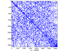
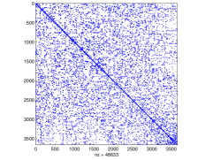
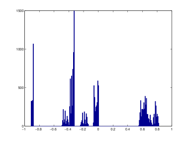
The numbers of nonzero entries are A𝐴A and B𝐵B are 145,899145899145,899 and 48,6334863348,633, respectively. The eigenvalues of the pencil are ranging from λmin=2.7395×10¹³subscript𝜆𝑚𝑖𝑛2.7395superscript1013\lambda_{min}=-2.7395\!\times\!10^{-13} to λmax=0.0325subscript𝜆𝑚𝑎𝑥0.0325\lambda_{max}=0.0325. Fig. 4 displays the sparsity patterns of A,B𝐴𝐵A,B as well as the histogram of the eigenvalues of (A,B)𝐴𝐵(A,B).

Refer to caption Refer to caption Refer to caption
(i) Sparsity of A𝐴A (ii) Sparsity of B𝐵B (iii) Histogram of eigenvalues
Fig. 4: For the earth’s normal mode matrix pencil, the sparsity pattern of A𝐴A, B𝐵B and the histogram of the eigenvalues of (A,B)𝐴𝐵(A,B) with 250250250 bins.

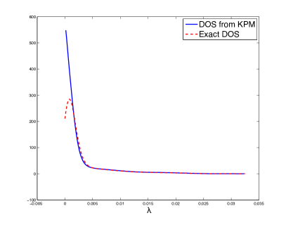
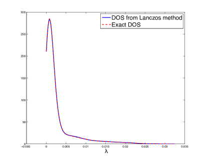
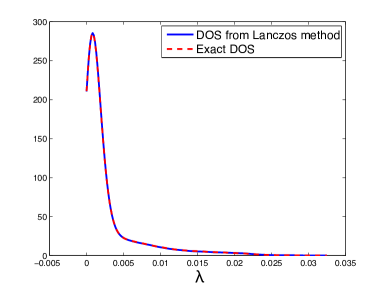
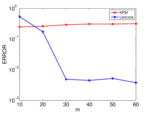
In Fig. 5, we first compare the computed accuracy of the KPM with that of the Lanczos method when the number of random vector nnevsubscript𝑛𝑛𝑒𝑣n_{nev} was fixed at 505050. The Cholesky factorization of B𝐵B was used for operations involving B𝐵B. We observe that the Lanczos method outperforms the KPM when m𝑚m varies from 202020 to 606060. This is because the eigenvalues of this pencil are clustered near the left endpoint of the spectrum (See Fig. 4 (iii)) and the KPM method has a hard time capturing this cluster (See Fig. 6).
Refer to caption

Fig. 5: A comparison of approximation errors of the KPM and Lanczos method applied to the earth’s normal mode matrix pencil for different m𝑚m values. The Cholesky factorization is performed for operations involving B𝐵B and nnevsubscript𝑛𝑛𝑒𝑣n_{nev} is fixed at 505050.
Refer to caption
Refer to caption
Fig. 6: For the earth’s normal mode matrix pencil, the computed DOS by the KPM (left) and the Lanczos method (right) when m=30𝑚30m=30 and nnev=50subscript𝑛𝑛𝑒𝑣50n_{nev}=50, compared to the exact DOS. Cholesky factorization is performed for operations involving B𝐵B.

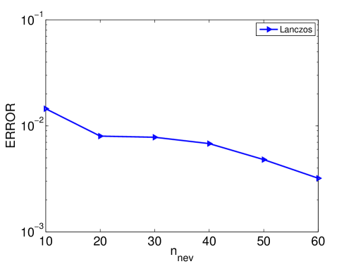
Fig. 7 shows the error of the Lanczos method with an increasing number of random vectors nnevsubscript𝑛𝑛𝑒𝑣n_{nev} and fixed m=30𝑚30m=30. It indicates that a large number of nnevsubscript𝑛𝑛𝑒𝑣n_{nev} helps reduce the error through the randomization.
Refer to caption

Fig. 7: For the earth’s normal mode pencil, the error of the Lanczos method with respect to an increasing number of random vectors nnevsubscript𝑛𝑛𝑒𝑣n_{nev} when m=30𝑚30m=30. Cholesky factorization is performed for operations involving B𝐵B.

Then we consider replacing the Cholesky factorization of B𝐵B with Chebyshev polynomial approximations gk1(B)subscript𝑔subscript𝑘1𝐵g_{k_{1}}(B) and qk2(B)subscript𝑞subscript𝑘2𝐵q_{k_{2}}(B) as proposed in Section 2.1. One way to determine the degree of gk1subscript𝑔subscript𝑘1g_{k_{1}} (or gk2subscript𝑔subscript𝑘2g_{k_{2}}) is to use the theoretical result of Theorem 3. However, the theorem has a parameter ρ𝜌\rho which is free and the selection of optimal ρ𝜌\rho may be harder than the selection of kisubscript𝑘𝑖k_{i} by simpler means. Since g(t)𝑔𝑡g(t), q(t)𝑞𝑡q(t) and their approximations are smooth and a simple heuristic is to select kisubscript𝑘𝑖k_{i} to be the smallest number for which the computed (ggk1)/gsubscriptnorm𝑔subscript𝑔subscript𝑘1𝑔\|(g-g_{k_{1}})/g\|_{\infty} and (qqk2)/qsubscriptnorm𝑞subscript𝑞subscript𝑘2𝑞\|(q-q_{k_{2}})/q\|_{\infty} are small enough. To evaluate the norm we can discretize the interval under consideration very finely (higher degrees will require more points). This will yield an estimate rather than an exact norm and this is enough for practical purposes.

For the original matrix pencil (A,B)𝐴𝐵(A,B), the eigenvalues of B𝐵B are inside [3.80e+07,1.46e+10]3.80𝑒071.46𝑒10[3.80e\!+\!07,1.46e\!+\!10] and κ(B)=382.91𝜅𝐵382.91\kappa(B)=382.91. In this case, we can estimate the convergence based on ρ1=[κ+1+2]/[κ1]=1.0750subscript𝜌1delimited-[]𝜅12delimited-[]𝜅11.0750\rho_{1}=[\sqrt{\kappa+1}+\sqrt{2}]/[\sqrt{\kappa-1}]=1.0750. Since ρ1subscript𝜌1\rho_{1} is close to 111, one should expect a slow convergence for gk1(B)subscript𝑔subscript𝑘1𝐵g_{k_{1}}(B) (or qk2(B)subscript𝑞subscript𝑘2𝐵q_{k_{2}}(B)) to B1superscript𝐵1B^{-1} (or B1/2superscript𝐵12B^{-1/2}). In Table 1, we report the computed norms (ggk)/gsubscriptnorm𝑔subscript𝑔𝑘𝑔\|(g-g_{k})/g\|_{\infty} and (qqk)/qsubscriptnorm𝑞subscript𝑞𝑘𝑞\|(q-q_{k})/q\|_{\infty} when k𝑘k increases from 303030 to 606060. As we can see, the error associated with gksubscript𝑔𝑘g_{k} is larger than 103superscript10310^{\!-\!3} even when k𝑘k reaches 606060.

Degree k𝑘k (ggk)/gsubscriptnorm𝑔subscript𝑔𝑘𝑔\|(g-g_{k})/g\|_{\infty} (qqk)/qsubscriptnorm𝑞subscript𝑞𝑘𝑞\|(q-q_{k})/q\|_{\infty}
30 8.62×1018.62superscript1018.62\!\times\!10^{-1} 1.92×1021.92superscript1021.92\!\times\!10^{-2}
40 3.10×1013.10superscript1013.10\!\times\!10^{-1} 6.00×1036.00superscript1036.00\!\times\!10^{-3}
50 1.12×1011.12superscript1011.12\!\times\!10^{-1} 2.00×1032.00superscript1032.00\!\times\!10^{-3}
60 4.01×1024.01superscript1024.01\!\times\!10^{-2} 6.45×1046.45superscript1046.45\!\times\!10^{-4}
Table 1: Computed error norms for the order k𝑘k Chebyshev polynomial approximations to g=1/λ𝑔1𝜆g\!=\!1/\lambda and q=1/λ𝑞1𝜆q\!=\!1/\sqrt{\lambda} on the interval [3.8017×107,1.4557×1010]3.8017superscript1071.4557superscript1010[3.8017\!\times\!10^{7},1.4557\!\times\!10^{10}], which contains the spectrum of the original mass matrix B𝐵B.

We then applied the diagonal scaling technique to the mass matrix B𝐵B. The eigenvalues of D1/2BD1/2superscript𝐷12𝐵superscript𝐷12D^{-1/2}BD^{-1/2} are now inside [0.5479,2.500]0.54792.500[0.5479,2.500] and κ(D1/2BD1/2)=4.5629𝜅superscript𝐷12𝐵superscript𝐷124.5629\kappa(D^{-1/2}BD^{-1/2})=4.5629. In this case, ρ1=1.9988subscript𝜌11.9988\rho_{1}=1.9988 and gk1(B)subscript𝑔subscript𝑘1𝐵g_{k_{1}}(B) and qk2(B)subscript𝑞subscript𝑘2𝐵q_{k_{2}}(B) converge much faster. This is confirmed in Table 2 where the error norms are smaller than 6×1066superscript1066\!\times\!10^{\!-6\!} for both approximations when k𝑘k reaches 12.

Degree k𝑘k (ggk)/gsubscriptnorm𝑔subscript𝑔𝑘𝑔\|(g-g_{k})/g\|_{\infty} (qqk)/qsubscriptnorm𝑞subscript𝑞𝑘𝑞\|(q-q_{k})/q\|_{\infty}
6 2.60×1022.60superscript1022.60\!\times\!10^{-2} 3.73×1043.73superscript1043.73\!\times\!10^{-4}
8 3.36×1043.36superscript1043.36\!\times\!10^{-4} 4.32×1054.32superscript1054.32\!\times\!10^{-5}
10 4.42×1054.42superscript1054.42\!\times\!10^{-5} 5.13×1065.13superscript1065.13\!\times\!10^{-6}
12 5.80×1065.80superscript1065.80\!\times\!10^{-6} 6.19×1076.19superscript1076.19\!\times\!10^{-7}
Table 2: Computed error norms for the order k𝑘k Chebyshev polynomial approximations to g=1/λ𝑔1𝜆g\!=\!1/\lambda and q=1/λ𝑞1𝜆q\!=\!1/\sqrt{\lambda} on the interval [0.5479,2.500]0.54792.500[0.5479,2.500], which contains the spectrum of the mass matrix B𝐵B after diagonal scaling.

Fig. 8 shows the error of the Lanczos method when the operations B1vsuperscript𝐵1𝑣B^{-1}v and B1/2vsuperscript𝐵12𝑣B^{-1/2}v are approximated by gk1(B)vsubscript𝑔subscript𝑘1𝐵𝑣g_{k_{1}}(B)v and qk2(B)vsubscript𝑞subscript𝑘2𝐵𝑣q_{k_{2}}(B)v, respectively. The number of sample vectors nnevsubscript𝑛𝑛𝑒𝑣n_{nev} was fixed at 505050 and the degree m𝑚m was fixed at 303030. The degrees of gk1subscript𝑔subscript𝑘1g_{k_{1}} and qk2subscript𝑞subscript𝑘2q_{k_{2}} are determined to be the smallest integers for which the following inequalities hold

(ggk1)/gτ,(qqk2)/qτ.formulae-sequencesubscriptnorm𝑔subscript𝑔subscript𝑘1𝑔𝜏subscriptnorm𝑞subscript𝑞subscript𝑘2𝑞𝜏\|(g-g_{k_{1}})/g\|_{\infty}\leq\tau,\quad\|(q-q_{k_{2}})/q\|_{\infty}\leq\tau. (59)

Although the exact DOS curve is indistinguishable from those obtained from the Lanczos method, the error actually decreases as we reduce the value of τ𝜏\tau. The errors are 1.41×1021.41superscript1021.41\!\times\!10^{-2}, 5.61×1035.61superscript1035.61\!\times\!10^{-3}, 4.70×1034.70superscript1034.70\!\times\!10^{-3} and 4.30×1034.30superscript1034.30\!\times\!10^{-3} when τ=101,102,103𝜏superscript101superscript102superscript103\tau=10^{-1},10^{-2},10^{-3} and 104superscript10410^{-4}, respectively. In the following experiments, we will fix τ𝜏\tau at 103superscript10310^{-3} to select the degree for gk1subscript𝑔subscript𝑘1g_{k_{1}} and qk2subscript𝑞subscript𝑘2q_{k_{2}} based on (59).

Refer to caption Refer to caption
(i) τ=101𝜏superscript101\tau=10^{-1} (ii) τ=102𝜏superscript102\tau=10^{-2}
Refer to caption Refer to caption
(iii) τ=103𝜏superscript103\tau=10^{-3} (iv) τ=104𝜏superscript104\tau=10^{-4}
Fig. 8: For the earth’s normal mode matrix pencil, the computed DOS by the Lanczos method when m=30𝑚30m=30 and nnev=50subscript𝑛𝑛𝑒𝑣50n_{nev}=50, compared to the exact DOS. The operations B1vsuperscript𝐵1𝑣B^{-1}v and B1/2vsuperscript𝐵12𝑣B^{-1/2}v are approximated by gk1(B)vsubscript𝑔subscript𝑘1𝐵𝑣g_{k_{1}}(B)v and qk2(B)vsubscript𝑞subscript𝑘2𝐵𝑣q_{k_{2}}(B)v, respectively. The degrees k1subscript𝑘1k_{1} and k2subscript𝑘2k_{2} are selected to be the smallest integers for which (59) hold. The approximation errors are 1.41×1021.41superscript1021.41\!\times\!10^{-2}, 5.61×1035.61superscript1035.61\!\times\!10^{-3}, 4.70×1034.70superscript1034.70\!\times\!10^{-3} and 4.30×1034.30superscript1034.30\!\times\!10^{-3} when τ𝜏\tau equals 101superscript10110^{-1}, 102superscript10210^{-2}, 103superscript10310^{-3} and 104superscript10410^{-4}, respectively.

5.2 An example from a Tight-Binding calculation

The second example is from the Density Functional-based Tight Binding (DFTB) calculations (Downloaded from http://faculty.smu.edu/yzhou/data/matrices.htm). The matrices A𝐴A and B𝐵B have dimension n=17,493𝑛17493n=17,493. The matrix A𝐴A has 3,927,77739277773,927,777 nonzero elements while B𝐵B has 3,926,40539264053,926,405 nonzero elements. The eigenvalues of the pencil are ranging from λmin=0.9138subscript𝜆𝑚𝑖𝑛0.9138\lambda_{min}=-0.9138 to λmax=0.8238subscript𝜆𝑚𝑎𝑥0.8238\lambda_{max}=0.8238.

Compared with the earth’s normal mode matrix pencil, both A,B𝐴𝐵A,B in this TFDB matrix pair are much denser. Fig. 9 displays the sparsity patterns of B𝐵B and of its Cholesky factor, where nz𝑛𝑧nz stands for the number of non-zeros. Even with the help of AMD ordering [1], the number of non-zeros in the Cholesky factor of B𝐵B still reaches 48,309,8574830985748,309,857, which amounts to having 5.5233×1035.5233superscript1035.5233\!\times\!10^{3} non-zeros per row/column. This will cause two issues. First, a huge amount of memory may be needed to store the factors for a similar problem of larger dimension. Second, applying these factors is also very inefficient. These issues limit the use of Cholesky factorization for realistic large-scale calculations. On the other hand, after diagonal scaling the matrix B𝐵B has eigenvalues in the remarkably tight interval [0.5756, 1.4432]0.57561.4432[0.5756,\ 1.4432], which allows a polynomial of degree as low as 666 for gk1subscript𝑔subscript𝑘1g_{k_{1}} and 555 for qk2subscript𝑞subscript𝑘2q_{k_{2}} when τ=103𝜏superscript103\tau=10^{-3}. Thus, we will only test the KPM and Lanczos method with Chebyshev polynomial approximation techniques for this problem.
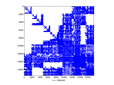
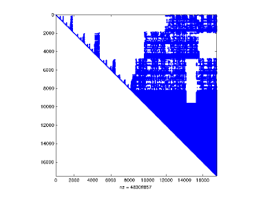
Refer to caption
Refer to caption
Fig. 9: The sparsity patterns of the matrix B𝐵B (left) and its Cholesky factor (right) for the TFDB matrix pencil. AMD ordering is applied to B𝐵B to reduce the number of non-zeros in its factors.

In the experiment, we fixed m=30𝑚30m=30 and nnev=50subscript𝑛𝑛𝑒𝑣50n_{nev}=50 in both methods. Fig. 10 shows that the quality of the computed DOS by the KPM method is clearly not as good as the one obtained from the Lanczos method. The error for the KPM is 0.27340.27340.2734 while the error for the Lanczos method is only 0.00580.00580.0058. This is because the spectrum of (A,B)𝐴𝐵(A,B) has four heavy clusters, which causes difficulties for polynomial-based methods to capture the corresponding peaks on the DOS curve.
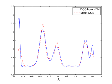
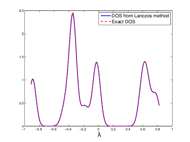
Refer to caption
Refer to caption

Refer to caption

Fig. 10: For the TFDB matrix pencil, the computed DOS by the KPM (upper left) and Lanczos method (upper right) when m=30𝑚30m=30 and nnev=50subscript𝑛𝑛𝑒𝑣50n_{nev}=50, compared to the exact DOS and the histogram of the eigenvalues with 200200200 bins (lower middle). Chebyshev polynomial approximations are used for operations involving B𝐵B.

5.3 Application: Slicing the spectrum

This section discusses the spectrum slicing techniques implemented in the EVSL package [9]. First, the Lanczos method is invoked to get an approximate DOS ϕ~~italic-ϕ\tilde{\phi} of the input matrix pencil (A,B)𝐴𝐵(A,B):

ϕ~(t)=1sk=1si=1mai(k)gσ(tθi(k))withgσ(t)=12πσet22σ2.formulae-sequence~italic-ϕ𝑡1𝑠superscriptsubscript𝑘1𝑠superscriptsubscript𝑖1𝑚superscriptsubscript𝑎𝑖𝑘subscript𝑔𝜎𝑡superscriptsubscript𝜃𝑖𝑘withsubscript𝑔𝜎𝑡12𝜋𝜎superscript𝑒superscript𝑡22superscript𝜎2\tilde{\phi}(t)=\frac{1}{s}\sum_{k=1}^{s}\sum_{i=1}^{m}a_{i}^{(k)}g_{\sigma}(t-{\theta_{i}^{(k)}})\ \ \text{with}\ \ g_{\sigma}(t)=\frac{1}{\sqrt{2\pi}\sigma}e^{\frac{-t^{2}}{2\sigma^{2}}}. (60)

Suppose the users would like to compute all the eigenvalues located inside a target interval [a,b]𝑎𝑏[a,\ b] as well as their associated eigenvectors with nssubscript𝑛𝑠n_{s} slices. The interval [a,b]𝑎𝑏[a,\ b] will first be finely discretized with N+1𝑁1N+1 evenly spaced points x0=a<x1<<xN1<xN=bsubscript𝑥0𝑎subscript𝑥1subscript𝑥𝑁1subscript𝑥𝑁𝑏x_{0}=a\!<\!x_{1}\!<\!\ldots\!<\!x_{N-1}\!<\!x_{N}=b, followed by the evaluation of ϕ~i:=ϕ~(xi)assignsubscript~italic-ϕ𝑖~italic-ϕsubscript𝑥𝑖\tilde{\phi}_{i}:=\tilde{\phi}(x_{i}) at each point xisubscript𝑥𝑖x_{i}.

Then a numerical integration scheme is used to approximate the following integral based on the computed {ϕ~i}subscript~italic-ϕ𝑖\{\tilde{\phi}_{i}\}

yiaxiϕ~(t)𝑑t.subscript𝑦𝑖superscriptsubscript𝑎subscript𝑥𝑖~italic-ϕ𝑡differential-d𝑡y_{i}\approx\int_{a}^{x_{i}}\tilde{\phi}(t)dt.

Each yisubscript𝑦𝑖y_{i} serves an approximation to the number of eigenvalues falling inside [a,xi]𝑎subscript𝑥𝑖[a,\ x_{i}]. In particular, we know there are roughly yNsubscript𝑦𝑁y_{N} eigenvalues inside [a,b]𝑎𝑏[a,\ b] and should expect an ideal partitioning yielding yN/nssubscript𝑦𝑁subscript𝑛𝑠y_{N}/n_{s} eigenvalues per slice.

The endpoints {ti}subscript𝑡𝑖\{t_{i}\} are identified as a subset of xisubscript𝑥𝑖x_{i}. Start with t0=x0subscript𝑡0subscript𝑥0t_{0}=x_{0}. The next ti+1subscript𝑡𝑖1t_{i+1} for i=0,,K2𝑖0𝐾2i=0,\ldots,K-2 is found by testing a sequence of xjsubscript𝑥𝑗x_{j} starting with ti=xksubscript𝑡𝑖subscript𝑥𝑘t_{i}=x_{k} until yjyksubscript𝑦𝑗subscript𝑦𝑘y_{j}-y_{k} is approximately equal to yK/nssubscript𝑦𝐾subscript𝑛𝑠y_{K}/n_{s}, yielding the point ti+1=xjsubscript𝑡𝑖1subscript𝑥𝑗t_{i+1}=x_{j}. In the end, the points {ti}subscript𝑡𝑖\{t_{i}\} separate [a,b]𝑎𝑏[a,\ b] into nssubscript𝑛𝑠n_{s} slices.

We illustrate the efficiency of this slicing mechanism with one example. The test problem is to partition the interval [0.003, 0.01]0.0030.01[0.003,\ 0.01] into 555 slices for the earth’s normal mode matrix pencil. Based on Fig. 6, we know that eigenvalues are distributed unevenly within this interval. Therefore, a naive uniform partitioning in which all sub-intervals have the same width will cause some slices to contain many more eigenvalues than others. We fixed m𝑚m at 303030 and varied the number of sample vectors nnevsubscript𝑛𝑛𝑒𝑣n_{nev} to estimate the DOS for this matrix pencil. The resulting partitioning results are tabulated in Table 3. As we can see, even a small number nnevsubscript𝑛𝑛𝑒𝑣n_{nev} can still provide a reasonable partitioning for the purpose of balancing the memory usage associated with each slice.

nnev=10subscript𝑛𝑛𝑒𝑣10n_{nev}=10 nnev=20subscript𝑛𝑛𝑒𝑣20n_{nev}=20 nnev=30subscript𝑛𝑛𝑒𝑣30n_{nev}=30
i𝑖i [ti,ti+1]subscript𝑡𝑖subscript𝑡𝑖1[t_{i},\ t_{i+1}] nisubscript𝑛𝑖n_{i} [ti,ti+1]subscript𝑡𝑖subscript𝑡𝑖1[t_{i},\ t_{i+1}] nisubscript𝑛𝑖n_{i} [ti,ti+1]subscript𝑡𝑖subscript𝑡𝑖1[t_{i},\ t_{i+1}] nisubscript𝑛𝑖n_{i}
1 [0.0030, 0.0036]0.00300.0036[0.0030,\ 0.0036] 848484 [0.0030, 0.0036]0.00300.0036[0.0030,\ 0.0036] 848484 [0.0030, 0.0036]0.00300.0036[0.0030,\ 0.0036] 848484
2 [0.0036, 0.0045]0.00360.0045[0.0036,\ 0.0045] 909090 [0.0036, 0.0045]0.00360.0045[0.0036,\ 0.0045] 909090 [0.0036, 0.0045]0.00360.0045[0.0036,\ 0.0045] 909090
3 [0.0045, 0.0059]0.00450.0059[0.0045,\ 0.0059] 105105105 [0.0045, 0.0059]0.00450.0059[0.0045,\ 0.0059] 105105105 [0.0045, 0.0060]0.00450.0060[0.0045,\ 0.0060] 113113113
4 [0.0059, 0.0077]0.00590.0077[0.0059,\ 0.0077] 113113113 [0.0059, 0.0078]0.00590.0078[0.0059,\ 0.0078] 119119119 [0.0060, 0.0079]0.00600.0079[0.0060,\ 0.0079] 115115115
5 [0.0077, 0.0100]0.00770.0100[0.0077,\ 0.0100] 110110110 [0.0078, 0.0100]0.00780.0100[0.0078,\ 0.0100] 104104104 [0.0079, 0.0100]0.00790.0100[0.0079,\ 0.0100] 989898
Table 3: Partitioning [0.003, 0.010]0.0030.010[0.003,\ 0.010] into 555 slices [ti,ti+1]subscript𝑡𝑖subscript𝑡𝑖1[t_{i},\ t_{i+1}] for the earth’s normal mode matrix pencil. The computational times for the Lanczos method are 0.530.530.53s, 0.960.960.96s and 1.581.581.58s as the number of sample vectors nnevsubscript𝑛𝑛𝑒𝑣n_{nev} increases from 101010 to 303030. nisubscript𝑛𝑖n_{i} is the exact number of eigenvalues located inside the i𝑖ith partitioned slice [ti,ti+1]subscript𝑡𝑖subscript𝑡𝑖1[t_{i},\ t_{i+1}].

6 Conclusion

Algorithms that require only matrix-vector multiplications can offer enormous advantages over those that rely on factorizations. This has been observed for polynomial filtering techniques for eigenvalue problems [10, 18], and it has also just been illustrated in this paper which described two methods to estimate spectral densities of matrix pencils. These two methods use Chebyshev polynomial approximation techniques to approximate the operations involving B𝐵B and so they only operate on (A,B)𝐴𝐵(A,B) through matrix-vector multiplications.

The bounds that were established suggest that the Lanczos method may converge twice as fast as the KPM method under some assumptions and it was confirmed experimentally to produce more accurate estimation when the spectrum contains clusters. The proposed methods are being implemented in C in the EVSL package [9] and will be made available in the next release.

This study suggested that it is also possible to compute eigenvalues and vectors of matrix pairs without any factorization. Theorem 6 indicates that rough approximations of the eigenpairs can be obtained by using a low-degree polynomial for B1/2superscript𝐵12B^{-1/2}. These approximations can be improved in a number of ways, e.g., by a Rayleigh-Ritz, or a subspace iteration-type procedure. We plan on exploring this approach in our future work.

References

  • [1] P. R. Amestoy, T. A. Davis, and I. S. Duff, Algorithm 837: An approximate minimum degree ordering algorithm, ACM Trans. Math. Software, 30 (2004), pp. 381–388.
  • [2] T. Ando, E. Chow, Y. Saad, and J. Skolnick, Krylov subspace methods for computing hydrodynamic interactions in brownian dynamics simulations, J. Chem. Phys., 137 (2012), p. 064106.
  • [3] E. G. Boman, K. Deweese, and J. R. Gilbert, An empirical comparison of graph laplacian solvers, 2016 Proceedings of the Eighteenth Workshop on Algorithm Engineering and Experiments (ALENEX), pp. 174–188.
  • [4] D. Cai, E. Chow, Y. Xi, and Y. Saad, SMASH: Structured matrix approximation by separation and hierarchy., Preprint ys-2016-10, Dept. Computer Science and Engineering, University of Minnesota, Minneapolis, MN, (2016).
  • [5] J. Chen, M. Anitescu, and Y. Saad, Computing f(a)b via least squares polynomial approximations, 33 (2011), pp. 195–222.
  • [6] K. Dong and D. Bindel, Modified kernel polynomial method for estimating graph spectra, in SIAM Network Science 2015 (poster), May 2015.
  • [7] D. A. Drabold and O. F. Sankey, Maximum entropy approach for linear scaling in the electronic structure problem, Phys. Rev. Lett., 70 (1993), pp. 3631–3634.
  • [8] A. Weiße, G. Wellein, A. Alvermann, and H. Fehske, The kernel polynomial method, Rev. Mod. Phys., 78 (2006), pp. 275–306.
  • [9] Eigenvalues slicing library. http://www.cs.umn.edu/similar-to\simsaad/software/EVSL/.
  • [10] H. R. Fang and Y. Saad, A filtered Lanczos procedure for extreme and interior eigenvalue problems, SIAM J. Scient. Comput., 34 (2012), pp. A2220–A2246.
  • [11] G. H. Golub and G. Meurant, Matrices, moments and quadrature, in IN NUMERICAL ANALYSIS, 1994, pp. 105–156.
  • [12] G. H. Golub and J. H. Welsch, Calculation of Gauss quadrature rule, Math. Comp., 23 (1969), pp. 221–230.
  • [13] L. Greengard and V. Rokhlin, A fast algorithm for particle simulations, J. Comput. Phys., 73 (1987), pp. 325–348.
  • [14] N. Higham, Functions of Matrices, Society for Industrial and Applied Mathematics, 2008.
  • [15] M. F. Hutchinson, A stochastic estimator of the trace of the influence matrix for Laplacian smoothing splines, Commun. Stat. Simul. Comput., 18 (1989), pp. 1059–1076.
  • [16] V. Kalantzis, R. Li, and Y. Saad, Spectral schur complement techniques for symmetric eigenvalue problems, Electron. Trans. Numer. Anal., 45 (2016), pp. 305–329.
  • [17] L. Kamenski, W. Huang, and H. Xu, Conditioning of finite element equations with arbitrary anisotropic meshes, Math. Comput., 83 (2014), pp. 2187–2211.
  • [18] R. Li, Y. Xi, E. Vecharynski, C. Yang, and Y. Saad, A Thick-Restart Lanczos algorithm with polynomial filtering for Hermitian eigenvalue problems, SIAM J. Sci. Comput., 38 (2016), pp. A2512–A2534.
  • [19] L. Lin, Randomized estimation of spectral densities of large matrices made accurate, Numer. Math., 136 (2017), pp. 183–213.
  • [20] L. Lin, Y. Saad, and C. Yang, Approximating spectral densities of large matrices, SIAM Review, 58 (2016), pp. 34–65.
  • [21] Y. Nakatsukasa, Absolute and relative weyl theorems for generalized eigenvalue problems, Linear Algebra Appl., 432 (2010), pp. 242 – 248.
  • [22] G. A. Parker, W. Zhu, Y. Huang, D.K. Hoffman, and D. J. Kouri, Matrix pseudo-spectroscopy: iterative calculation of matrix eigenvalues and eigenvectors of large matrices using a polynomial expansion of the Dirac delta function, Comput. Phys. Commun., 96 (1996), pp. 27–35.
  • [23] Y. Saad, Numerical Methods for Large Eigenvalue Problems, SIAM, Philadelpha, 2011.
  • [24] G. Schofield, J. R. Chelikowsky, and Y. Saad, A spectrum slicing method for the kohn–sham problem, Comput. Phys. Commun., 183 (2012), pp. 497 – 505.
  • [25] J. Shi and M. V. de Hoop, A note on the parallel computation of earth’s normal modes via structured factorization, Preceedings of the Project Review, Geo-Mathematical Imaging Group, (2016), pp. 223–236.
  • [26] J. Shi, M. V. de Hoop, R. Li, Y. Xi, and Y. Saad., Fast eigensolver for computing earth’s normal modes, in Proceedings of the Project Review, Geo-Mathematical Imaging Group, vol. 2, 2017, pp. 317–345.
  • [27] R. N. Silver and H. Röder, Densities of states of mega-dimensional Hamiltonian matrices, Int. J. Mod. Phys. C, 5 (1994), pp. 735–753.
  • [28]  , Calculation of densities of states and spectral functions by Chebyshev recursion and maximum entropy, Phys. Rev. E, 56 (1997), p. 4822.
  • [29] R. N. Silver, H. Röder, A. F. Voter, and J. D. Kress, Kernel polynomial approximations for densities of states and spectral functions, J. Comput. Phys., 124 (1996), pp. 115–130.
  • [30] J. M. Tang and Y. Saad, A probing method for computing the diagonal of a matrix inverse, Numer. Lin. Alg. Appl., 19 (2012), pp. 485–501.
  • [31] L. N. Trefethen, Approximation Theory and Approximation Practice (Other Titles in Applied Mathematics), Society for Industrial and Applied Mathematics, Philadelphia, PA, USA, 2012.
  • [32] S. Ubaru and Y. Saad, Fast methods for estimating the numerical rank of large matrices, in Proceedings of the 33rd International Conference on International Conference on Machine Learning - Volume 48, ICML’16, JMLR.org, 2016, pp. 468–477.
  • [33] S. Ubaru, A.-K. Seghouane, and Y. Saad, Improving the incoherence of a learned dictionary via rank shrinkage, Neural Computation, (2017), pp. 263–285.
  • [34] L.-W. Wang, Calculating the density of states and optical-absorption spectra of large quantum systems by the plane-wave moments method, Phys. Rev. B, 49 (1994), p. 10154.
  • [35] A. Wathen, Realistic eigenvalue bounds for the Galerkin mass matrix, IMA J. Numer. Anal., 7 (1987), pp. 449–457.
  • [36] A. Wathen and T. Rees, Chebyshev semi-iteration in preconditioning for problems including the mass matrix., Electron. Trans. Numer. Anal., 34 (2008), pp. 125–135.
  • [37] Y. Xi and Y. Saad, Computing partial spectra with least-squares rational filters, SIAM J. Sci. Comput., 38 (2016), pp. A3020–A3045.
  • [38] Y. Zhou, Y. Saad, M. L. Tiago, and J. R. Chelikowsky, Parallel self-consistent-field calculations via Chebyshev-filtered subspace acceleration, Phy. Rev. E, 74 (2006), p. 066704.