A large-scale analysis of racial disparities
in police stops across the United States

Abstract

To assess racial disparities in police interactions with the public, we compiled and analyzed a dataset detailing over 60 million state patrol stops conducted in 20 U.S. states between 2011 and 2015. We find that black drivers are stopped more often than white drivers relative to their share of the driving-age population, but that Hispanic drivers are stopped less often than whites. Among stopped drivers—and after controlling for age, gender, time, and location—blacks and Hispanics are more likely to be ticketed, searched, and arrested than white drivers. These disparities may reflect differences in driving behavior, and are not necessarily the result of bias. In the case of search decisions, we explicitly test for discrimination by examining both the rate at which drivers are searched and the likelihood searches turn up contraband. We find evidence that the bar for searching black and Hispanic drivers is lower than for searching whites. Finally, we find that legalizing recreational marijuana in Washington and Colorado reduced the total number of searches and misdemeanors for all race groups, though a race gap still persists. We conclude by offering recommendations for improving data collection, analysis, and reporting by law enforcement agencies.

Introduction

More than 20 million Americans are stopped each year for traffic violations, making this one of the most common ways in which the public interacts with the police (Langton and Durose, 2013). Due to a lack of comprehensive data, it has been difficult to rigorously assess the manner and extent to which race plays a role in traffic stops (Epp et al., 2014). The most widely cited national statistics come from the Police-Public Contact Survey (PPCS), which is based on a nationally representative sample of approximately 50,000 people who report having been recently stopped by the police (Bureau of Justice Statistics, 2014). In addition to such survey data, some local and state agencies have released periodic reports on traffic stops in their jurisdictions, and have also made their data available to researchers for analysis  (Antonovics and Knight, 2009; Simoiu et al., 2017; Anwar and Fang, 2006; Ridgeway and MacDonald, 2009; Ridgeway, 2006; Ryan, 2016; Rojek et al., 2004; Smith and Petrocelli, 2001; Warren et al., 2006; Hetey et al., 2016; Seguino and Brooks, 2017; Voigt et al., 2017). While useful, these datasets provide only a partial picture. For example, there is concern that the PPCS, like nearly all surveys, suffers from selection bias and recall errors. Data released directly by police departments are potentially more complete, but are available only for select agencies, are typically limited in what is reported, and are inconsistent across jurisdictions.

Here we analyze a unique dataset detailing more than 60 million state patrol stops conducted in 20 states between 2011 and 2015. We compiled this dataset through a series of public records requests filed with all 50 states, and we are redistributing these records in a standardized form to facilitate future analysis. Our statistical analysis of these records proceeds in three steps. First, we quantify racial disparities in stop rates and post-stop outcomes. Adjusting for age, gender, location and year, we find that black drivers are stopped more often than white drivers relative to their share of the driving-age population, but find that Hispanic drivers are stopped less often than whites. After being stopped, black and Hispanic drivers are more likely than whites to be ticketed, searched, and arrested. Such disparities may stem from a combination of factors—including differences in driving behavior—and are not necessarily the result of racial bias. In the second phase of our analysis, we investigate the degree to which these differences may result from discrimination, focusing on search decisions. By examining both the rate at which searches occur and the success rate of these searches, we find evidence that the bar for searching black and Hispanic drivers is lower than for searching white drivers. Finally, we examine the effects of drug policy on stop outcomes. We find that legalizing recreational marijuana in Washington and Colorado reduced both search and misdemeanor rates for white, black, and Hispanic drivers, though a relative gap persists. We conclude by suggesting best-practices for data collection, analysis, and reporting by law enforcement agencies.

Compiling a national database of traffic stops

Figure 1: We collected detailed information on over 60 million state patrol stops conducted in 20 states between 2011 and 2015. An additional 11 states provided data that are insufficient to assess racial disparities, and 19 states have not provided any data (including Hawaii and Alaska).

Data collection

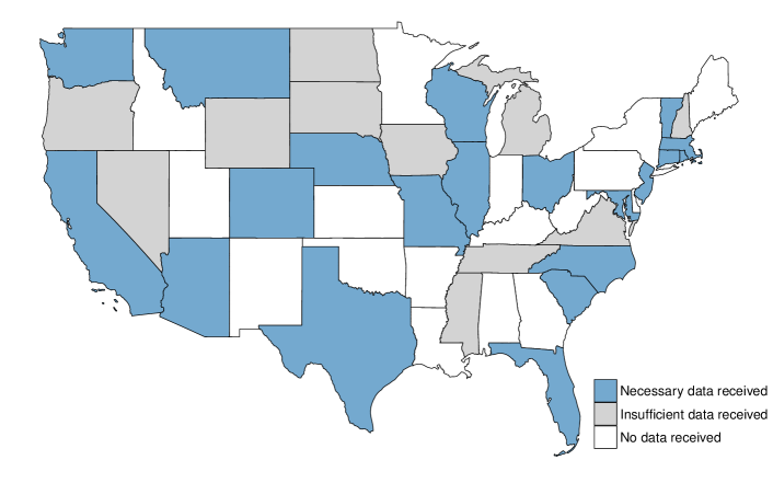
To assemble a national dataset of traffic stops, we first identified which state law enforcement agencies electronically maintain traffic stop records that, at a minimum, include the race of the stopped driver. Of the 50 state agencies, 7 did not respond to our request for information or did not disclose whether any data were collected; an additional 9 agencies do not compile stop records electronically or reported that they were unable to send their data to us in electronic form; and 3 state agencies keep electronic records but do not track the race of stopped drivers (see Table A1 for details). For the remaining 31 states, we filed public records requests for detailed information on each stop conducted since 2005.

To date, we have collected data on approximately 136 million state patrol stops in 31 states. Of these, we exclude 11 states from our analysis because the obtained data were insufficient to assess racial disparities (e.g., the race of the stopped driver was not regularly recorded, or only a non-representative subset of stops was provided). In the remaining 20 states that we consider, 18 provided data for each individual stop. In the other two—Missouri and Nebraska—only summary data were provided, but these summaries were sufficiently granular to allow for statistical analysis. For consistency in our analysis, we restrict to stops occurring in 2011–2015, as many states did not provide data on earlier stops. We also limit our analysis to drivers classified as white, black or Hispanic, as there are relatively few recorded stops of drivers in other race groups. Our primary dataset thus consists of 63.7 million state patrol stops from 20 states (Figure 1).

Data normalization

Each state provided the stop data in idiosyncratic formats with varying levels of specificity, and so we used a variety of automated and manual procedures to create the final dataset. For each recorded stop, we attempted to extract and normalize the date and time of the stop; the county or state patrol district in which the stop took place; the race, gender and age of the driver; the stop reason; whether a search was conducted; the legal justification for the search (e.g., “probable cause” or “consent”); whether contraband was found during a search; and the stop outcome (e.g., a citation or an arrest). We describe our procedures for normalizing each of these covariates in the Appendix. As indicated in Table 1, the availability of information varies significantly across states. We therefore restrict each of our specific analyses to the corresponding subset of states for which we have the required fields.

In many states, more than one row in the raw data appeared to refer to the same stop. For example, in several states each row referred to one violation, not one stop. We detected and reconciled such duplicates by inspecting columns with granular values. For example, in Colorado we counted two rows as duplicates if they had the same officer identification code, officer first and last name, driver first and last name, driver birth date, stop location (precise to the milepost marker), and stop date and time (precise to the minute).

State Stops Time Stop Stop Stop Driver Driver Stop Search Search Contraband Stop Range Date Time Location Gender Age Reason Conducted Type Found Outcome 1 Arizona 2,039,781 2011-2015 $\bullet$ $\bullet$ $\bullet$ $\bullet$ $\bullet$ $\bullet$ $\bullet$ 2 California 19,012,414 2011-2015 $\bullet$ $\bullet$ $\bullet$ $\bullet$ $\bullet$ $\bullet$ $\bullet$ 3 Colorado 1,674,619 2011-2015 $\bullet$ $\bullet$ $\bullet$ $\bullet$ $\bullet$ $\bullet$ $\bullet$ $\bullet$ $\bullet$ 4 Connecticut 310,969 2013-2015 $\bullet$ $\bullet$ $\bullet$ $\bullet$ $\bullet$ $\bullet$ $\bullet$ $\bullet$ $\bullet$ $\bullet$ 5 Florida 4,002,547 2011-2015 $\bullet$ $\bullet$ $\bullet$ $\bullet$ $\bullet$ $\bullet$ $\bullet$ $\bullet$ $\bullet$ 6 Illinois 1,528,340 2011-2015 $\bullet$ $\bullet$ $\bullet$ $\bullet$ $\bullet$ $\bullet$ $\bullet$ $\bullet$ $\bullet$ 7 Maryland 578,613 2011-2014 $\bullet$ $\bullet$ $\bullet$ $\bullet$ $\bullet$ $\bullet$ 8 Massachusetts 1,773,546 2011-2015 $\bullet$ $\bullet$ $\bullet$ $\bullet$ $\bullet$ $\bullet$ $\bullet$ $\bullet$ 9 Missouri 1,906,797 2011-2015 $\bullet$ $\bullet$ 10 Montana 547,115 2011-2015 $\bullet$ $\bullet$ $\bullet$ $\bullet$ $\bullet$ $\bullet$ $\bullet$ $\bullet$ $\bullet$ 11 Nebraska 840,764 2011-2014 $\bullet$ 12 New Jersey 2,069,123 2011-2015 $\bullet$ $\bullet$ $\bullet$ $\bullet$ $\bullet$ $\bullet$ 13 North Carolina 3,500,180 2011-2015 $\bullet$ $\bullet$ $\bullet$ $\bullet$ $\bullet$ $\bullet$ $\bullet$ $\bullet$ $\bullet$ 14 Ohio 4,660,935 2011-2015 $\bullet$ $\bullet$ $\bullet$ $\bullet$ $\bullet$ 15 Rhode Island 229,691 2011-2015 $\bullet$ $\bullet$ $\bullet$ $\bullet$ $\bullet$ $\bullet$ $\bullet$ $\bullet$ $\bullet$ $\bullet$ 16 South Carolina 3,696,801 2011-2015 $\bullet$ $\bullet$ $\bullet$ $\bullet$ $\bullet$ $\bullet$ $\bullet$ 17 Texas 10,239,721 2011-2015 $\bullet$ $\bullet$ $\bullet$ $\bullet$ $\bullet$ $\bullet$ $\bullet$ $\bullet$ $\bullet$ 18 Vermont 250,949 2011-2015 $\bullet$ $\bullet$ $\bullet$ $\bullet$ $\bullet$ $\bullet$ $\bullet$ $\bullet$ $\bullet$ $\bullet$ 19 Washington 4,053,099 2011-2015 $\bullet$ $\bullet$ $\bullet$ $\bullet$ $\bullet$ $\bullet$ $\bullet$ $\bullet$ $\bullet$ $\bullet$ 20 Wisconsin 827,028 2011-2015 $\bullet$ $\bullet$ $\bullet$ $\bullet$ $\bullet$ $\bullet$ $\bullet$ $\bullet$ $\bullet$ Total 63,743,032

Table 1: Availability of data in the 20 states comprising our primary analysis, where for each column a solid circle signifies data are available for at least 70% of the stops. For all states except Illinois, North Carolina, and Rhode Island, “stop location” refers to county; for these three states, it refers to a similarly granular location variable, as described above.

Error correction

The raw data in many states contain errors. We ran numerous automated checks to detect and correct these where possible, although some errors likely remain due to the complex nature of the data. For example, after examining the distribution of recorded values in each state, we discovered a spurious density of stops in North Carolina listed as occurring at precisely midnight. As the value “00:00” was likely used to indicate missing information, we treated it as such.

Past work suggests that Texas state patrol officers incorrectly recorded many Hispanic drivers as white. To investigate and correct for this issue, we impute Hispanic ethnicity from surnames in the three states for which we have name data: Texas, Arizona, and Colorado. To do so, we use a dataset from the U.S. Census Bureau that estimates the racial and ethnic distribution of people with a given surname, for surnames occurring at least 100 times (Word et al., 2008). To increase the matching rate, we perform minor string edits to the names, including removing punctuation and suffixes (e.g., “Jr.” and “II”), and consider only the longest word in multi-part surnames. Following past work (Word and Perkins, 1996; Melendres v. Arpaio, 2009), we define a name as “Hispanic-affiliated” if at least 75% of people with that name identify as Hispanic, according to the 2000 Census; we note that 90% of those with Hispanic-affiliated names identify as Hispanic. Among drivers with Hispanic-affiliated names, the proportion labeled as Hispanic in the raw data is considerably lower in Texas (37%) than in either Arizona (79%) or Colorado (70%), corroborating past results. Though imperfect, we re-categorize as “Hispanic” all drivers in Texas with Hispanic-affiliated names who were originally labeled “white” or had missing race data.

Our complete data cleaning pipeline is extensive, requiring subjective decisions and thousands of lines of code. For transparency and reproducibility, we have released the raw data, the standardized data, and code to clean and analyze the records at https://openpolicing.stanford.edu.

Stop rates and post-stop outcomes

We begin our analysis by examining the extent to which there are racial disparities in stop, citation, search, and arrest rates. The disparities we discuss below likely result from a combination of complex factors, and do not necessarily reflect racial bias. Regardless of the mechanism, however, we quantify these disparities in order to better understand the differential impact policing has on minority communities.

Figure 2: Stops per person of driving age, stratified by race and location, where points are sized proportional to the number of stops. The plots cover 16 states for which we have location data. Within location, black drivers are often stopped more often than white drivers; Hispanic drivers are generally stopped at similar rates as whites.

Stop rates

We first estimate the rate at which white, black, and Hispanic drivers are stopped, relative to their share of the driving-age population (Smith and Petrocelli, 2001). Although there are a variety of benchmarks one might consider (Lange et al., 2005; Alpert et al., 2004; Engel and Calnon, 2004), the driving-age population has the unique distinction of being readily available in nearly every jurisdiction, and it is accurately estimated by the U.S. Census Bureau; we note, however, that this benchmark does not account for possible race-specific differences in driving behavior, including amount of time spent on the road and adherence to traffic laws.

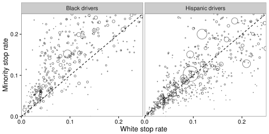
Figure 2 shows stop rates of black and Hispanic drivers relative to whites, disaggregated by location. Each point in the plot corresponds to either the county or similar geographic unit in which the stop was made. We find that Hispanics are stopped at similar rates as whites in most jurisdictions; black drivers, however, are stopped more often than whites in over 80% of the locations we consider.

We next estimate race-specific stop rates after adjusting for driver demographics (age and gender), stop location, and stop year; age was binned into the categories 16–19, 20–29, 30–39, 40–49, and 50+ years-old. In our primary analysis, we fit a negative binomial regression, where we benchmark to the census-estimated driving-age population:

$$y_{rag\ell y}\sim\text{NegBin}\left(n_{rag\ell y}e^{\mu+\alpha_{r}+\beta_{a}+\gamma_{g}+\delta_{\ell}+\epsilon_{y}},\phi\right)$$

where $y_{rag\ell y}$ is the observed number of stops in a group defined by race, age, gender, location, and year, $n_{rag\ell y}$ is the corresponding census benchmark, and $\alpha_{r}$ are the key race coefficients (we set $\alpha_{\text{white}}=0$). The negative binomial distribution is parameterized such that if $Y\sim\text{NegBin}(\mu,\phi)$, then $\mathbb{E}[Y]=\mu$ and $\text{Var}[Y]=\mu+\mu^{2}/\phi$. The parameter $\phi$ allows for overdispersion, and is estimated from the data.

Table 2 (first column) shows the estimated race, gender and age coefficients; we further estimate $\hat{\phi}=3.9$. After controlling for gender, age, location, and year, we find that blacks are stopped at 1.4 times the rate at which whites are stopped ($e^{0.37}=1.4$), and Hispanics are stopped at 0.7 times the white stop rate ($e^{-0.40}=0.7$). To help interpret these numbers, Table 3 shows stop rates for a typical 20-29 year-old male driver: the per-capita stop rate is 0.42 for blacks, 0.29 for whites, and 0.19 for Hispanics.

As shown in Figure 2, Hispanic drivers are stopped at similar rates as whites when controlling only for location. But Hispanic drivers are more likely to be young, and young drivers are more likely to be stopped. As a result, after additionally adjusting for age (and other covariates) in the regression above, we find Hispanics are stopped at a lower rate than whites. This lower estimated rate is consistent with self-reports collected as part of the PPCS (Bureau of Justice Statistics, 2014). With the PPCS data, we used logistic regression to estimate the likelihood a respondent would report having been stopped by the police while driving, where we controlled for the respondent’s race, age, gender, and size of city. We found that Hispanic respondents were less likely than white drivers to report having been stopped (odds ratio = 0.85). This result is in line with a similar analysis of the same PPCS data (Medina Jr, 2016).

To check the robustness of the observed racial disparities, we additionally fit stop rate regressions using a Poisson model with sandwich errors, and using a quasi-Poisson model (Ver Hoef and Boveng, 2007; Gardner et al., 1995). We report these results in Table LABEL:tab:all_regression_coefficients (first three rows). The signs of the race coefficients are the same under all three specifications, but the estimated effect sizes are somewhat larger in the negative binomial model than in the two Poisson models (both of which necessarily yield identical coefficients). We note that it is common for Poisson and negative binomial formulations to produce somewhat different effect sizes (Ver Hoef and Boveng, 2007).

	Stop	Citation	Search	Consent search	Arrest
Black	0.37 (0.01)	0.18 (0.00)	0.73 (0.01)	0.77 (0.03)	0.65 (0.01)
Hispanic	-0.40 (0.01)	0.29 (0.00)	0.54 (0.01)	0.62 (0.02)	0.69 (0.01)
Male	0.72 (0.00)	0.08 (0.00)	0.58 (0.01)	0.86 (0.02)	0.43 (0.01)
Age 20-29	0.65 (0.01)	-0.13 (0.01)	0.13 (0.01)	-0.38 (0.03)	0.38 (0.01)
Age 30-39	0.47 (0.01)	-0.35 (0.01)	-0.06 (0.01)	-0.79 (0.03)	0.30 (0.01)
Age 40-49	0.25 (0.01)	-0.47 (0.01)	-0.37 (0.01)	-1.20 (0.04)	-0.04 (0.01)
Age 50+	-0.53 (0.01)	-0.68 (0.01)	-0.80 (0.01)	-1.82 (0.04)	-0.47 (0.01)

Table 2: Coefficients and standard errors for stop rate and post-stop outcome models.

	White	Black	Hispanic
Stop rate	0.29	0.42	0.19
Speeding citation	72%	75%	77%
Search	1.3%	2.7%	2.3%
Consent search	0.1%	0.3%	0.3%
Arrest	2.8%	5.3%	5.5%

Table 3: Model-estimated rates for a typical 20-29 year-old male. The “speeding citation” outcome corresponds to receiving a citation rather than a warning (or no penalty) when pulled over for speeding. Negative binomial regression is used for stop rate (first row), benchmarked to the driving-age population; logistic regression is used for all other analyses. The stop rate regression includes controls for age, gender, stop location, and stop year; all other regressions additionally include controls for stop quarter, weekday, and hour (binned into three-hour segments).

Citation, search, and arrest rates

Stop rates are a natural starting point but are inherently difficult to interpret, in part because results can be sensitive to the benchmark used. (We note that there are no readily available alternatives to the driving-age population.) We thus now consider post-stop outcomes, starting with the rates at which white and minority drivers receive citations rather than warnings when pulled over for speeding.

We use logistic regression to estimate racial disparities in the probability a driver stopped for speeding is given a citation as opposed to a warning (or no penalty at all). In addition to driver age and gender, location, and year, we control for stop quarter, stop weekday, and stop hour, binned into eight 3-hour segments. (In the case of stop rates, we used negative binomial and Poisson models since we were estimating total counts; we could not control for time in that case because we lacked time-specific population benchmarks.) Table 2 (second column) shows the estimated race, gender and age coefficients. We find that black drivers have 19% higher odds of receiving a citation than white drivers, and Hispanics have 34% higher odds than whites. For typical young male drivers, Table 3 shows that 72% of whites stopped for speeding receive a citation, compared to 75% and 77% for black and Hispanic drivers, respectively.

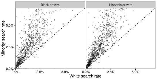
Next, we examine search rates. After stopping a driver, officers may search both driver and vehicle for drugs, weapons, and other contraband when they suspect more serious criminal activity. Aggregating across all states for which we have search data, white drivers are searched in 2.0% of stops, compared to 3.5% of stops for black motorists and 3.8% for Hispanic motorists. Across jurisdiction, Figure 3 (top row) shows that black and Hispanic motorists are consistently searched at higher rates than white drivers. After controlling for stop location, date and time, and driver age and gender—via logistic regression, as above—we find that black and Hispanic drivers have approximately twice the odds of being searched relative to white drivers (2.1 and 1.7, respectively, as shown in Table 2).

Figure 3: Search rates (top) and arrest rates (bottom) by race and location among stopped drivers. In nearly every area, minorities are searched and arrested more often than whites. The search data cover 16 states, comprising a total of 56 million stops, and the arrest data include 40 million stops in 13 states.

We now consider the subset of searches conducted with consent, where officers must seek permission from drivers to search their vehicles. (In contrast, probable cause searches do not require consent, but legally demand a high standard of evidence.) We find that minority drivers are more likely than whites to undergo consent searches in the seven states for which we have reliable data (Colorado, Florida, Massachusetts, Maryland, North Carolina, Texas, and Washington); controlling for stop location, date and time, and driver age and gender, we find that black drivers have 2.2 times the odds of whites and Hispanic drivers have 1.9 times the odds of whites of undergoing a consent search (Table 2).

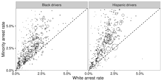
Finally, we examine arrest rates. In aggregate, black drivers are arrested in 2.8% of stops and Hispanic drivers in 3.4% of stops, compared to 1.7% for white drivers. Again controlling for driver age and gender, stop date and time, and stop location, we find that black drivers have 1.9 times the odds of being arrested, and Hispanic drivers have 2.0 times the odds of being arrested compared to white drivers (Figure 3 and Table 2).

To assess the robustness of our results on citation, search, and arrest rates, we fit logistic regression models with five different sets of control variables, as described in Table LABEL:tab:all_regression_coefficients: (1) driver race only; (2) driver race and county; (3) driver race, age, gender, and county; (4) driver race, county, and stop time; and (5) driver race, age, gender, county, and stop time. These five models were fit on the largest set of states for which the relevant information was available. In nearly every case, the estimated race coefficients were positive and significant, indicating that black and Hispanic drivers were cited, searched, and arrested more often than white drivers. There was one exception: we found a negative coefficient (-0.11) for Hispanic drivers when estimating the likelihood of receiving a speeding citation when controlling only for race. This outlier occurs because Texas has an especially high fraction of Hispanic drivers and an especially low rate of citations. Finally, we confirmed that these racial disparities persist when we alter the set of stops analyzed: we find qualitatively similar results when we fit our models only on speeding stops; when we eliminate searches incident to arrest; and when we fit models on each state separately.

Testing for bias in search decisions

When stopped, black and Hispanic drivers are more likely to be issued citations, more likely to be searched, and more likely to be arrested. These disparities, however, are not necessarily the product of discrimination. Minority drivers might, for example, carry contraband at higher rates than whites, and so elevated search rates may result from routine police work. We now investigate whether bias plays a role in search decisions, a class of actions amenable to statistical analysis.

The outcome test

To start, we apply the outcome test, originally proposed by Becker (1957, 1993) to circumvent omitted variable bias in traditional tests of discrimination. The outcome test is based not on the search rate, but on the hit rate: the proportion of searches that successfully turn up contraband. Becker argued that even if minority drivers are more likely to carry contraband, absent discrimination searched minorities should still be found to have contraband at the same rate as searched whites. If searches of minorities are less often successful than searches of whites, it suggests that officers are applying a double standard, searching minorities on the basis of less evidence.

Figure 4: Hit rates (top) and inferred search thresholds (bottom) by race and location, covering 470,000 searches in 9 states. Across locations, the inferred thresholds for searching black and Hispanic drivers are typically lower than those for searching white drivers. Despite these lower inferred search thresholds, hit rates for blacks are comparable to hit rates for whites, possibly due to the problem of infra-marginality in outcome tests.

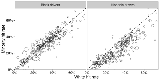
In Figure 4 (top row), we plot hit rates by race and location for the nine states (Colorado, Connecticut, Illinois, North Carolina, Rhode Island, South Carolina, Texas, Washington, and Wisconsin) for which we have the necessary information: the race of the driver, the location of the stop, whether a search was conducted, and whether contraband was found. Across jurisdictions, we consistently see that searches of Hispanic drivers are less successful than those of white drivers. However, searches of white and black drivers generally have comparable hit rates. Aggregating across location, searches of Hispanic drivers yield contraband 22% of the time, compared to 28% for searches of white and black drivers. In computing these aggregate statistics, we include Missouri and Maryland, which provide search and contraband data but not stop location, and Vermont, which has too few stops of minorities to be included in our county-level analysis in Figure 4. The outcome test thus indicates that search decisions may be biased against Hispanic drivers but not black drivers.

The threshold test

The outcome test is intuitively appealing, but it is not a perfect barometer of bias; in particular, it suffers from the problem of infra-marginality (Ayres, 2002; Anwar and Fang, 2006). To illustrate this shortcoming, suppose that there are two, easily distinguishable types of white drivers: those who have a 5% chance of carrying contraband, and those who have a 75% chance of carrying contraband. Likewise assume that black drivers have either a 5% or 50% chance of carrying contraband. If officers search drivers who are at least 10% likely to be carrying contraband, then searches of whites will be successful 75% of the time whereas searches of blacks will be successful only 50% of the time. Thus, although the search criterion is applied in a race-neutral manner, the hit rate for blacks is lower than the hit rate for whites, and the outcome test would (incorrectly) conclude searches are biased against black drivers. The outcome test can similarly fail to detect discrimination when it is present.

To mitigate this limitation of outcome tests, the threshold test has been proposed as a more robust means for detecting discrimination (Simoiu et al., 2017; Pierson et al., 2017). This test aims to estimate race-specific probability thresholds above which officers search drivers—for example, the 10% threshold in the hypothetical situation above. Even if two race groups have the same observed hit rate, the threshold test may find that one group is searched on the basis of less evidence, indicative of discrimination. To accomplish this task, the test simultaneously estimates race-specific search thresholds and risk distributions that are consistent with the observed search and hit rates across all jurisdictions. The threshold test can thus be seen as a hybrid between outcome and benchmark analysis.

Here we present a brief overview of the threshold test as applied in our setting; see Simoiu et al. (2017) for a more complete description. For each stop $i$, we assume that we observe: (1) the race of the driver, $r_{i}$; (2) the stop location, $d_{i}$; (3) whether the stop resulted in a search, indicated by $S_{i}\in\{0,1\}$; and (4) whether the stop resulted in a hit, indicated by $H_{i}\in\{0,1\}$. We applied the threshold test separately on each state having the requisite data, and limited to stop locations (e.g., counties) with at least 1,000 stops. If more than 100 locations in a state had over 1,000 stops, we considered only the 100 locations with the most stops.

The threshold test is based on a stylized model of officer behavior. During each stop, officers observe a myriad of contextual factors—including the age and gender of the driver, the stop time and location, and behavioral indicators of nervousness or evasiveness. We assume that officers distill these factors down to a single number that represents the likelihood the driver is carrying contraband, and then conduct a search if that probability exceeds a fixed race- and location-specific threshold. Since there is uncertainty in who is pulled over in any given stop, the probability of finding contraband is modeled as a random draw from a race- and location-specific signal distribution. The threshold test jointly estimates these search thresholds and signal distributions using a hierarchical Bayesian model, as described below. Under this model, lower search thresholds for one group relative to another are interpreted as evidence of taste-based discrimination (Becker, 1957).

Formally, for each stop $i$, we assume $(S_{i},H_{i})$ is stochastically generated in three steps.

1. Given the race $r_{i}$ of the driver and the stop location $d_{i}$, the officer observes a signal $p_{i}\sim\text{beta}(\phi_{r_{i}d_{i}},\lambda_{r_{i}d_{i}})$, where $\phi_{r_{i}d_{i}}$ and $\lambda_{r_{i}d_{i}}$ are defined by:

   $$\phi_{rd}=\textrm{logit}^{-1}(\phi_{r}+\phi_{d})$$

   and

   $$\lambda_{rd}=\exp(\lambda_{r}+\lambda_{d}).$$

   The beta distribution is parameterized by its mean $\phi_{rd}$ and total count parameter $\lambda_{rd}$. In terms of the standard count parameters $\alpha$ and $\beta$ of the beta distribution, $\phi=\alpha/(\alpha+\beta)$ and $\lambda=\alpha+\beta$. Thus, $\phi_{rd}$ is the overall probability that a stopped driver of race $r$ in location $d$ has contraband, and $\lambda_{rd}$ characterizes the heterogeneity of guilt across stopped drivers of that race in that location. These parameters of the beta distributions are in turn functions of parameters that depend separately on race and location.

2. $S_{i}=1$ (i.e., a search is conducted) if and only if $p_{i}\geq t_{r_{i}d_{i}}$. The thresholds $t_{rd}$ are the key parameters of interest.

3. If $S_{i}=1$, then $H_{i}\sim\text{Bernoulli}(p_{i})$; otherwise $H_{i}=0$.

This generative process is parameterized by $\{\phi_{r}\}$, $\{\lambda_{r}\}$, $\{\phi_{d}\}$, $\{\lambda_{d}\}$ and $\{t_{rd}\}$. To complete the model specification, we place weakly informative priors on $\phi_{r}$, $\lambda_{r}$, $\phi_{d}$, and $\lambda_{d}$, and place a weakly informative hierarchical prior on $t_{rd}$. The hierarchical structure allows us to make reasonable inferences even for locations with a relatively small number of stops. Finally, we compute the posterior distribution of the parameters given the data.

Figure 5: Posterior predictive checks for search rates (top) and hit rates (bottom). Both plots indicate the fitted model captures key features of the data.

We estimate the posterior distribution of the parameters via Hamiltonian Monte Carlo (HMC) sampling (Neal, 1994; Duane et al., 1987), a form of Markov chain Monte Carlo sampling (Metropolis et al., 1953). We specifically use the No-U-Turn sampler (NUTS) (Hoffman and Gelman, 2014) as implemented in Stan (Carpenter et al., 2016), an open-source modeling language for full Bayesian statistical inference. To assess convergence of the algorithm, we sampled five Markov chains in parallel and computed the potential scale reduction factor $\hat{R}$ (Gelman and Rubin, 1992). We found that 2,500 warmup iterations and 2,500 sampling iterations per chain were sufficient for convergence, as indicated by $\hat{R}$ values less than $1.05$ for all parameters, as well as by visual inspection of the trace plots.

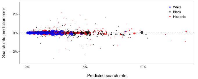
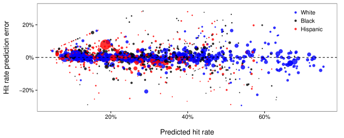
We apply posterior predictive checks (Gelman et al., 2014, 1996) to evaluate the extent to which the fitted model yields race- and location-specific search and hit rates that are in line with the observed data. For each department and race group, we compare the observed search and hit rates to their expected values under the assumed data-generating process with parameters drawn from the inferred posterior distribution. Specifically, we compute the posterior predictive search and hit rates as follows. During model inference, our Markov chain Monte Carlo sampling procedure yields $2,500\times 5=12,500$ draws from the joint posterior distribution of the parameters. For each parameter draw—consisting of $\{\phi_{r}^{*}\}$, $\{\lambda_{r}^{*}\}$, $\{\phi_{d}^{*}\}$, $\{\lambda_{d}^{*}\}$ and $\{t_{rd}^{*}\}$—we analytically compute the search and hit rates $s_{rd}^{*}$ and $h_{rd}^{*}$ for each race-location pair implied by the data-generating process with those parameters. Finally, we average these search and hit rates over all 12,500 posterior draws. Figure 5 compares the model-predicted search and hit rates to the actual, observed values. Each point in the plot corresponds to a single race-location group, where groups are sized by number of stops. The fitted model recovers the observed search rates almost perfectly across races and locations. The fitted hit rates also agree with the data well, with the largest groups exhibiting almost no error. These posterior predictive checks thus indicate that the fitted model captures key features of the observed data.

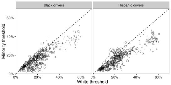
We now turn to the substantive implications of our threshold analysis. As shown in Figure 4 (bottom row), the threshold test indicates that the bar for searching black and Hispanic drivers is lower than for searching white drivers in nearly every location we consider. In aggregate, the inferred threshold for white drivers is 20%, compared to 16% for blacks and 14% for Hispanics. These aggregate thresholds are computed by taking a weighted average of location-specific thresholds, where weights are proportional to the total number of stops in each location. The 95% credible intervals for the aggregate, race-specific thresholds are non-overlapping: $(19\%,20\%)$ for white drivers, $(15\%,17\%)$ for black drivers, and $(13\%,14\%)$ for Hispanic drivers. Whereas the outcome test indicates discrimination only against Hispanic drivers, the threshold test suggests discrimination against both blacks and Hispanics. Consistent with past work (Simoiu et al., 2017), this difference appears to be driven by a small but disproportionate number of black drivers who have high inferred likelihood of carrying contraband. Thus, even though the threshold test finds the bar for searching black drivers is lower than for whites, these groups have similar hit rates.

The threshold test provides evidence of bias in search decisions. However, as with all tests of discrimination, there is a limit to what one can conclude from such statistical analysis alone. For example, if search policies differ not only across but also within jurisdictions, then the threshold test might mistakenly indicate discrimination where there is none. Additionally, if officers disproportionately suspect more serious criminal activity when searching black and Hispanic drivers compared to whites, then lower observed thresholds may stem from non-discriminatory police practices.

The effects of legalizing marijuana on stop outcomes

Figure 6: The proportion of stops that result in a drug-related misdemeanor (top) or search (bottom) before and after recreational marijuana was legalized in Colorado and Washington at the end of 2012 (indicated by the vertical lines). Subsequent to legalization, there is a substantial drop in search and misdemeanor rates. The dashed lines show fitted linear trends pre- and post-legalization.

Figure 7: In the twelve states where marijuana was not legalized, and for which we have the necessary search data, search rates do not fall at the end of 2012; this pattern further suggests that marijuana legalization caused the observed drop in search rates in Colorado and Washington.

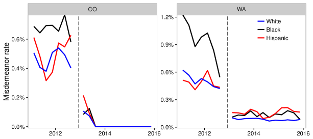
We conclude our analysis by investigating the effects of legalizing recreational marijuana on search and misdemeanor rates. We specifically examine Colorado and Washington, the two states in which marijuana was recently legalized and for which we have detailed data. As shown in Figure 6 (top) the number of drug-related misdemeanors in both states fell substantially after marijuana was legalized at the end of 2012, in line with expectations. In Colorado, we consider only misdemeanors for marijuana possession, and so the rate necessarily drops after legalization; in Washington, we include misdemeanors for any type of drug possession as more detailed information is not available, and so there are still some recorded drug misdemeanors post-legalization. Notably, since black drivers were more likely to be charged with such offenses prior to legalization, black drivers were also disproportionately impacted by the policy change. This finding is consistent with past work showing that marijuana laws disproportionately affect minorities (Mitchell and Caudy, 2015).

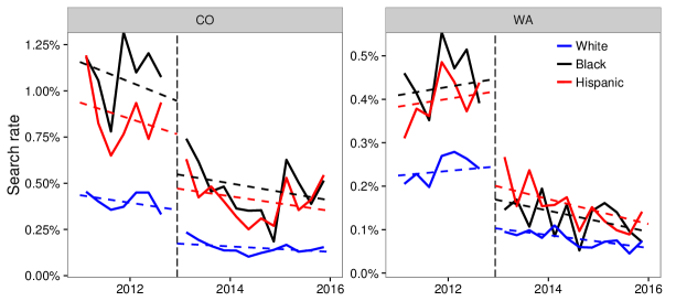
Because the policy change decriminalized an entire class of behavior (i.e., possession of minor amounts of marijuana), it is not surprising that drug offenses correspondingly decreased. It is less clear, however, how the change affected officer behavior more broadly. We find that after marijuana was legalized, the number of searches fell substantially in Colorado and Washington, (Figure 6, bottom), ostensibly because the policy change removed a common reason for conducting searches. In both states, we exclude searches incident to an arrest and other searches that are conducted as a procedural matter, irrespective of any suspicion of drug possession. Because black and Hispanic drivers were more likely to be searched prior to legalization, the policy change reduced the absolute gap in search rates between white and minority drivers; however, the relative gap persists, with minorities still more likely to be searched than whites. We further note that marijuana legalization has secondary impacts for law-abiding drivers, as fewer searches overall means fewer searches of innocent individuals. In the year after legalization in Colorado and Washington, 40% fewer drivers were searched with no contraband found than in the year before legalization.

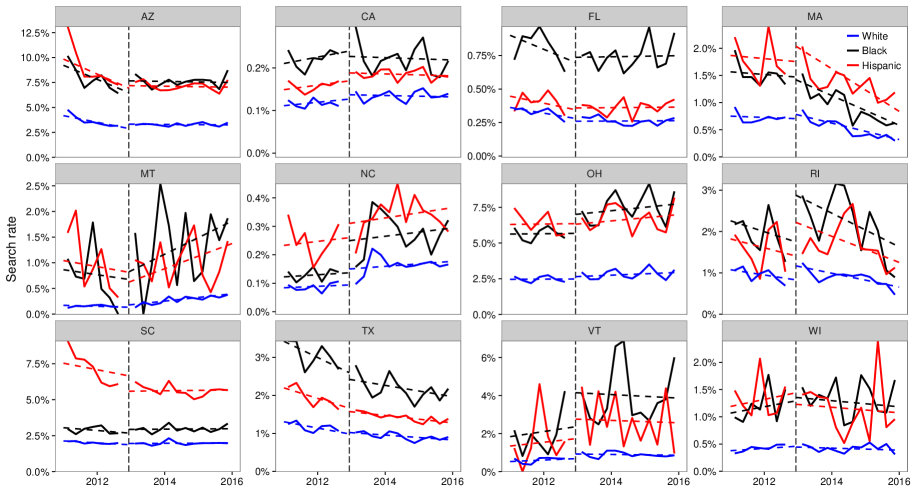
As shown in Figure 7, in the twelve states where marijuana was not legalized—and for which we have the necessary search data—search rates did not drop significantly at the end of 2012. This pattern further suggests that the observed drop in search rates in Colorado and Washington is due to marijuana legalization. To add quantitative detail to this visual result, we compute a simple difference-in-difference estimate (Angrist and Pischke, 2008). Specifically, we fit the following search model on the set of stops in the 14 states we consider here (Colorado, Washington, and the twelve non-legalization states in Figure 7):

$$\Pr(Y=1)=\textrm{logit}^{-1}\left(\sum_{s\in\text{state}}\beta_{s}I_{s}+\sum_{r\in\text{race}}\beta_{r}I_{r}+\beta_{t}\cdot t+\sum_{r\in\text{race}}\alpha_{r}I_{r}Z\right),$$

where $Y$ indicates whether a search was conducted, $\beta_{s}$ and $\beta_{r}$ are state and race fixed effects, and $\beta_{t}$ is a time trend, with $t$ a continuous variable in units of years since legalization (e.g., $t=0.5$ means 6 months post-legalization). The $Z$ term indicates “treatment” status; that is, $Z_{i}=1$ in Colorado and Washington for stops carried out during the post-legalization period, and $Z_{i}=0$ otherwise. Thus the key parameters of interest are the race-specific treatment effects $\alpha_{r}$. Table 4 lists coefficients for the fitted model. We find that $\alpha_{r}$ is large and negative for whites, blacks, and Hispanics, which again suggests the observed drop in searches in Colorado and Washington was due to the legalization of marijuana in those states.

	Coef.	s.e.
Effect of legalization on white drivers	-0.99	0.02
Effect of legalization on black drivers	-1.01	0.06
Effect of legalization on Hispanic drivers	-0.79	0.03
Time (years)	-0.02	0.00
Black driver	0.79	0.00
Hispanic driver	0.64	0.00

Table 4: Effects of legalizing recreational marijuana on search rates, as estimated with a difference-in-difference model. All race groups experienced a large drop in search rate.

Despite marijuana legalization decreasing search rates for all races, Figure 6 shows that the relative disparity between whites and minorities remains. We adapt the threshold test to assess the extent to which this disparity in search rates may reflect bias. Specifically, we estimate race-specific search thresholds pre- and post-legalization. To do so, we first divide the stops into pre- and post-legalization periods, indexed by $t\in\{\textrm{pre},\,\textrm{post}\}$. The equations in Section 4.2 are modified to allow race-dependent time variation in the signal distributions and thresholds:

$$\phi_{rdt} =\textrm{logit}^{-1}(\phi_{r}+\phi_{d}+\phi_{rt})$$

$$\lambda_{rdt} =\exp(\lambda_{r}+\lambda_{d}+\lambda_{rt})$$

$$t_{rdt} =t_{rd}+t_{rt},$$

where the new parameters $\phi_{rt}$, $\lambda_{rt}$, and $t_{rt}$ are set to 0 when $t=\textrm{pre}$, and given a weakly informative $\text{N}(0,1)$ prior otherwise. Inference in the model is performed separately for Colorado and Washington.

Figure 8: Inferred average thresholds faced by drivers of different races before and after marijuana legalization. Error bars show the 95% credible intervals of the posterior thresholds. In all cases minority drivers face a lower threshold than white drivers.

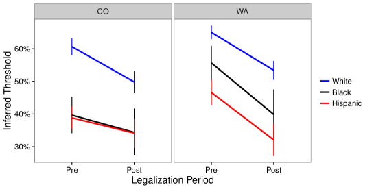
Examining the inferred thresholds (shown in Figure 8), we observe that whites drivers face consistently higher search thresholds than minority drivers, both before and after marijuana legalization. The data thus suggest that although overall search rates drop in Washington and Colorado, bias persists in search decisions.

Figure 8 also shows that the average threshold faced by all groups decreases after legalization (though not all drops are statistically significant). There are several possible explanations for this decrease. Officers may not have fully internalized the change of policy, searching people who would have been at risk of carrying contraband before legalization, but are no longer high risk now that marijuana is legal. Alternatively, or in addition, officers may now be focused on more serious offenses (such as drug trafficking), applying a lower threshold commensurate with the increase in the severity of the suspected crime. Finally, officers may have more resources after being relieved of the task of policing marijuana possession, freeing them to make searches with a lower chance of finding contraband.

Discussion

Our investigation of over 60 million state patrol stops across the United States reveals widespread racial disparities in stop, citation, search, and arrest rates. It is important to note, however, that such differences may stem from a variety of mechanisms, and are not necessarily the result of racial bias. Moving beyond these disparities, a threshold analysis indicates that black and Hispanic drivers are searched on the basis of less evidence than white drivers, suggestive of bias in search decisions. The recent legalization of recreational marijuana in Colorado and Washington reduced the absolute gap in search rates between whites and minorities—because search rates decreased for all groups—but the relative gap remained. A threshold test further suggests that minorities continue to face bias in search decisions post-legalization. In aggregate, our results lend insight into the differential impact of policing on minority communities nationwide.

Our study provides a unique perspective on working with large-scale policing data. We conclude by offering several recommendations for data collection, release, and analysis. At minimum, we encourage states to collect individual-level stop data that include the date and time of the stop; the location of the stop; the race, gender, and age of the driver; the stop reason; whether a search was conducted; the search type (e.g., “probable cause” or “consent”); whether contraband was found during a search; the stop outcome (e.g., a citation or an arrest); and the specific violation the driver was charged with. Most states collect only a subset of this information. There are also variables that are currently rarely collected but would be useful for analysis, such as indicia of criminal behavior, an officer’s rationale for conducting a search, and short narratives written by officers describing the incident. New York City’s UF-250 form for pedestrian stops is an example of how such information can be efficiently collected (Goel et al., 2016a; Mummolo, 2016).

Equally important to data collection is ensuring the integrity of the recorded information. We frequently encountered missing values and errors in the data (e.g., implausible values for a driver’s age and invalid racial categorizations). Automated procedures can be put in place to help detect and correct such problems. In most cases, the recorded race of the driver is based on the officer’s perception, rather than a driver’s self-categorization. While there are sound reasons for this practice, it increases the likelihood of errors, a problem we observed in the Texas state patrol data. To quantify and correct for this issue, police departments might regularly audit their data, possibly by comparing an officer’s perception of race to a third party’s judgment based on driver’s license photos for a random sample of stopped drivers.

Despite the existence of public records laws, seven states failed to respond to our repeated requests for information. We hope law enforcement agencies consider taking steps to make data more accessible to external researchers and to the public. Connecticut and North Carolina are at the forefront of opening up their data, providing online portals for anyone to download and analyze this information.

Finally, we hope that police departments start regularly analyzing their data and report the results of their findings. Such analyses might include estimates of stop, search, and hit rates, stratified by race, age, gender, and location; distribution of stop reasons by race; and trends over time. More ambitiously, departments could use their data to design statistically informed guidelines to encourage more consistent, efficient, and equitable decisions (Goel et al., 2016a, b). Many of these analyses can be automated and re-run regularly with little marginal effort. In conjunction with releasing the data underlying these analyses, we recommend the analysis code also be released to ensure reproducibility. Collecting, releasing, and analyzing police data are essential steps for increasing the effectiveness and equity of law enforcement, and for improving relations with the public through transparency.

Appendix

Below we describe the procedures we used to standardize each field in our data.

1. Stop location. The location of stops was encoded at varying levels of granularity across states, including police beat, city or town name, intersection, address, highway number and marker, county name, county FIPS code, district code, latitude and longitude coordinates, and highway patrol trooper zone. To provide a standard location coding, we aimed to map each stop to the county in which it occurred. For example, the data provided by Washington contained the highway type, number, and closest mile marker, which we first mapped to latitude and longitude coordinates using a publicly available dataset of highway marker locations; we then mapped the coordinates to counties using public shape files. Similarly, unidentified counties in Arizona were mapped to county using the highway the stop occurred on. For Connecticut, Massachusetts and Vermont, the counties were mapped using the police department that recorded the stop. For these states we found the county corresponding to the police department using the Google Maps API. In North Carolina, Illinois, and Rhode Island, no consistent county-level information was provided for state patrol stops. Therefore, we mapped stops to similarly granular location variables: for North Carolina we used district, for Illinois we used state patrol division, and for Rhode Island we used zone code. For North Carolina and Illinois we aggregated census statistics for the counties subsumed in the region to have a usable benchmark.

2. Driver race. We restrict our primary analysis to white, black, and Hispanic drivers. We specifically exclude stops of Asian and Native American drivers, as these groups were not sufficiently represented in our data to allow granular analysis. Some states provided ethnicity of the driver in addition to race; drivers with Hispanic ethnicity were considered Hispanic regardless of their recorded race, consistent with previous investigations. To aid future work, we classify drivers as “Asian” and “other” where possible—though these groups are not included in our main analysis. For example, Native American and Alaskan Native drivers were classified as “other”; South Asian and Pacific Islander drivers were classified as “Asian”.

3. Driver age. States provided either date of birth, birth year, or age of the driver. The age of the driver at the time of the stop was calculated by taking the difference between the stop date and the birth date of the driver, or stop year and birth year. If the inferred age of driver was less than 15 or greater than or equal to 100, we assumed the data were incorrect and treated age as missing in those cases.

4. Violation. Some states listed one violation per stop, while others provided multiple violations (e.g., there were up to twelve recorded in Washington). If multiple violation codes were provided, all were included in our standardized data. The granularity of violation codes also varied greatly, from two categories (e.g., speeding and seat belt violations in Massachusetts) to over 1,000 in Colorado. Some states provided violation data by referring to local state statute numbers, which we mapped to a text description of the violation by consulting state traffic laws. We developed a two-level hierarchy of violation categories, and standardized each violation reason using this rubric. Our violation categories are as follows: (1) license/registration (with subcategories for license, registration/plates, and paperwork); (2) speeding; (3) seat belt violations; (4) stop sign/light; (5) equipment (with a subcategory for head/taillight violations); (6) driving under the influence (DUI); (7) moving violations (with subcategories for “safe movement” and “cell phone”); and (8) truck violations. We coded violations using the most granular category possible. For states that had hundreds of violation codes, we mapped the most common ones until 95% of stops were accounted for.

5. Stop purpose. Some states distinguish between violation and stop purpose—the initial reason for the stop. When stop purpose was explicitly provided, it was placed in a separate column and normalized using the same values as the violation codes.

6. Stop outcome. Some states provided information on the outcome of the stop: for example, verbal warning, written warning, citation, summons, or arrest. In the case of speeding stops—which we specifically analyze—a stop was classified as a warning if either a warning or no penalty was given. A few states provided multiple outcomes for each stop, and in these cases, we recorded the most severe outcome—for example, if both a citation and a warning were given, the stop outcome was coded as a citation .

7. Search conducted. Many states provided a binary indicator for whether a search was conducted. In other cases we had to construct this field from other information in the data. For instance, North Carolina and South Carolina provided information on whether the driver, passenger, or vehicle was searched; we coded that a search was conducted if any of these three events occurred.

8. Search type. We standardize search types into categories which include, for example, consent, probable cause, incident to arrest, inventory, warrant, protective frisk, and K9 searches. Most of the standardization consisted of normalizing the language (e.g., “drug dog alert” and “any K9 Used for Search” were mapped to “K9 search”). Some states had multiple search reasons, others only one. If multiple search types were given, all were included in our standardized dataset.

9. Contraband found. As with the “search conducted” field, states often provided a binary indicator for whether contraband was found. In other cases, it is constructed from multiple binary flags. For example, in South Carolina, we say that contraband was found if any of the “Contraband”, “ContrabandDrugs,” “ContrabandDrugParaphenalia,”, “ContrabandWeapons”, or “ContrabandDesc” fields indicate that contraband was found. In some cases, it was indicated that contraband was found but no search was conducted. It is unclear whether a search was in fact conducted but not recorded, whether contraband was incorrectly marked, or whether contraband was discovered through a process other than a search (e.g., found near the vehicle). In these instances, we set the field value to “false”, and note that the choice affects only a small proportion of searches and does not qualitatively affect our results.

State	Data released	Used in analysis	Response status
Alabama			No response
Alaska			Does not collect
Arizona	$\bullet$	$\bullet$	Individual stop data received
Arkansas			No central database
California	$\bullet$	$\bullet$	Individual stop data received
Colorado	$\bullet$	$\bullet$	Individual stop data received
Connecticut	$\bullet$	$\bullet$	Individual stop data received
Delaware			Provided reports only
Florida	$\bullet$	$\bullet$	Individual stop data received
Georgia			Does not collect
Hawaii			No response
Idaho			Does not collect
Illinois	$\bullet$	$\bullet$	Individual stop data received
Indiana			No response
Iowa	$\bullet$		Incomplete race data
Kansas			Request denied
Kentucky			No central database
Louisiana			Request denied
Maine			No central database
Maryland	$\bullet$	$\bullet$	Individual stop data received
Massachusetts	$\bullet$	$\bullet$	Individual stop data received
Michigan	$\bullet$		Incomplete race data
Minnesota			Does not collect
Mississippi	$\bullet$		Incomplete race data
Missouri	$\bullet$	$\bullet$	Summary data received
Montana	$\bullet$	$\bullet$	Individual stop data received
Nebraska	$\bullet$	$\bullet$	Summary data received
Nevada	$\bullet$		Incomplete race data
New Hampshire	$\bullet$		Incomplete race data
New Jersey	$\bullet$	$\bullet$	Individual stop data received
New Mexico			No response
New York			No central database
North Carolina	$\bullet$	$\bullet$	Individual stop data received
North Dakota	$\bullet$		Provided citation data only
Ohio	$\bullet$	$\bullet$	Individual stop data received
Oklahoma			No response
Oregon	$\bullet$		Summary data received, not usable
Pennsylvania			Request denied
Rhode Island	$\bullet$	$\bullet$	Individual stop data received
South Carolina	$\bullet$	$\bullet$	Individual stop data received
South Dakota	$\bullet$		Missing race data
Tennessee	$\bullet$		Provided citation data only
Texas	$\bullet$	$\bullet$	Individual stop data received
Utah			Request denied
Vermont	$\bullet$	$\bullet$	Individual stop data received
Virginia	$\bullet$		Summary data received, not usable
Washington	$\bullet$	$\bullet$	Individual stop data received
West Virginia			No central database
Wisconsin	$\bullet$	$\bullet$	Individual stop data received
Wyoming	$\bullet$		Provided citation data only

Table A1: Status of responses to our public record requests, at time of writing.

References

- Alpert et al. (2004) Geoffrey Alpert, Michael Smith, and Roger Dunham. Toward a better benchmark: Assessing the utility of not-at-fault traffic crash data in racial profiling research. Justice Research and Policy, 6(1):43–69, 2004.
- Angrist and Pischke (2008) Joshua D Angrist and Jörn-Steffen Pischke. Mostly harmless econometrics: An empiricist’s companion. Princeton university press, 2008.
- Antonovics and Knight (2009) Kate Antonovics and Brian Knight. A new look at racial profiling: Evidence from the Boston police department. The Review of Economics and Statistics, 91(1):163–177, 2009.
- Anwar and Fang (2006) Shamena Anwar and Hanming Fang. An alternative test of racial prejudice in motor vehicle searches: Theory and evidence. The American Economic Review, 2006.
- Ayres (2002) Ian Ayres. Outcome tests of racial disparities in police practices. Justice Research and Policy, 4(1-2):131–142, 2002.
- Becker (1957) Gary Becker. The economics of discrimination. University of Chicago Press, 1957.
- Becker (1993) Gary Becker. Nobel lecture: The economic way of looking at behavior. Journal of Political Economy, pages 385–409, 1993.
- Bureau of Justice Statistics (2014) Bureau of Justice Statistics. Police-public contact survey, 2011. 2014. doi: 10.3886/ICPSR34276.v1.
- Carpenter et al. (2016) Bob Carpenter, Andrew Gelman, Matt Hoffman, Daniel Lee, Ben Goodrich, Michael Betancourt, Marcus A Brubaker, Jiqiang Guo, Peter Li, and Allen Riddell. Stan: A probabilistic programming language. Journal of Statistical Software, 2016.
- Duane et al. (1987) Simon Duane, Anthony D Kennedy, Brian J Pendleton, and Duncan Roweth. Hybrid Monte Carlo. Physics Letters B, 195(2):216–222, 1987.
- Engel and Calnon (2004) Robin Engel and Jennifer Calnon. Comparing benchmark methodologies for police-citizen contacts: Traffic stop data collection for the Pennsylvania State Police. Police Quarterly, 7(1):97–125, 2004.
- Epp et al. (2014) Charles Epp, Steven Maynard-Moody, and Donald Haider-Markel. Pulled over: How police stops define race and citizenship. University of Chicago Press, 2014.
- Gardner et al. (1995) William Gardner, Edward P Mulvey, and Esther C Shaw. Regression analyses of counts and rates: Poisson, overdispersed Poisson, and negative binomial models. Psychological bulletin, 118(3):392, 1995.
- Gelman and Rubin (1992) Andrew Gelman and Donald B Rubin. Inference from iterative simulation using multiple sequences. Statistical Science, pages 457–472, 1992.
- Gelman et al. (1996) Andrew Gelman, Xiao-Li Meng, and Hal Stern. Posterior predictive assessment of model fitness via realized discrepancies. Statistica Sinica, 6(4):733–760, 1996.
- Gelman et al. (2014) Andrew Gelman, John B Carlin, Hal S Stern, and Donald B Rubin. Bayesian data analysis. Taylor & Francis, 2nd edition, 2014.
- Goel et al. (2016a) Sharad Goel, Justin Rao, and Ravi Shroff. Precinct or prejudice? Understanding racial disparities in New York City’s stop-and-frisk policy. Annals of Applied Statistics, 2016a.
- Goel et al. (2016b) Sharad Goel, Justin Rao, and Ravi Shroff. Personalized risk assessments in the criminal justice system. The American Economic Review, 106(5):119–123, 2016b.
- Hetey et al. (2016) Rebecca Hetey, Benoît Monin, Amrita Maitreyi, and Jennifer Eberhardt. Data for change: A statistical analysis of police stops, searches, handcuffings, and arrests in oakland, calif., 2013-2014. Technical report, Stanford University, SPARQ: Social Psychological Answers to Real-World Questions, 2016.
- Hoffman and Gelman (2014) Matthew D Hoffman and Andrew Gelman. The No-U-Turn Sampler: Adaptively setting path lengths in Hamiltonian Monte Carlo. Journal of Machine Learning Research, 15(Apr):1593–1623, 2014.
- Lange et al. (2005) James Lange, Mark Johnson, and Robert Voas. Testing the racial profiling hypothesis for seemingly disparate traffic stops on the new jersey turnpike. Justice Quarterly, 22(2):193–223, 2005.
- Langton and Durose (2013) Lynn Langton and Matthew Durose. Police behavior during traffic and street stops, 2011. Technical report, U.S. Department of Justice, 2013.
- Medina Jr (2016) Michael A Medina Jr. Accounting for membership: an examination of the effects race, sex, and age has on police conduct and force during traffic stops. PhD thesis, Rutgers University–Camden Graduate School, 2016.
- Melendres v. Arpaio (2009) Melendres v. Arpaio. Melendres v. Arpaio, 2009. 598 F. Supp. 2d 1025 (D. Ariz. 2009).
- Metropolis et al. (1953) Nicholas Metropolis, Arianna W Rosenbluth, Marshall N Rosenbluth, Augusta H Teller, and Edward Teller. Equation of state calculations by fast computing machines. The Journal of Chemical Physics, 21(6):1087–1092, 1953.
- Mitchell and Caudy (2015) Ojmarrh Mitchell and Michael Caudy. Examining racial disparities in drug arrests. Justice Quarterly, 32(2):288–313, 2015.
- Mummolo (2016) Jonathan Mummolo. Modern police tactics, police-citizen interactions and the prospects for reform. Journal of Politics, 2016. Forthcoming.
- Neal (1994) Radford M Neal. An improved acceptance procedure for the hybrid Monte Carlo algorithm. Journal of Computational Physics, 111(1):194–203, 1994.
- Pierson et al. (2017) Emma Pierson, Sam Corbett-Davies, and Sharad Goel. Fast threshold tests for detecting discrimination. Preprint available at https://arxiv.org/abs/1702.08536, 2017.
- Ridgeway (2006) Greg Ridgeway. Assessing the effect of race bias in post-traffic stop outcomes using propensity scores. Journal of Quantitative Criminology, 22(1):1–29, 2006.
- Ridgeway and MacDonald (2009) Greg Ridgeway and John MacDonald. Doubly robust internal benchmarking and false discovery rates for detecting racial bias in police stops. Journal of the American Statistical Association, 104(486):661–668, 2009.
- Rojek et al. (2004) Jeff Rojek, Richard Rosenfeld, and Scott Decker. The influence of driver’s race on traffic stops in missouri. Police Quarterly, 7(1):126–147, 2004.
- Ryan (2016) Matt Ryan. Frisky business: race, gender and police activity during traffic stops. European Journal of Law and Economics, 41(1):65–83, 2016.
- Seguino and Brooks (2017) Stephanie Seguino and Nancy Brooks. Driving while black and brown in vermont. 2017.
- Simoiu et al. (2017) Camelia Simoiu, Sam Corbett-Davies, and Sharad Goel. The problem of infra-marginality in outcome tests for discrimination. Annals of Applied Statistics, 2017. Forthcoming.
- Smith and Petrocelli (2001) Michael Smith and Matthew Petrocelli. Racial profiling? a multivariate analysis of police traffic stop data. Police Quarterly, 4(1):4–27, 2001.
- Ver Hoef and Boveng (2007) Jay M Ver Hoef and Peter L Boveng. Quasi-Poisson vs. negative binomial regression: How should we model overdispersed count data? Ecology, 88(11):2766–2772, 2007.
- Voigt et al. (2017) Rob Voigt, Nicholas P Camp, Vinodkumar Prabhakaran, William L Hamilton, Rebecca C Hetey, Camilla M Griffiths, David Jurgens, Dan Jurafsky, and Jennifer L Eberhardt. Language from police body camera footage shows racial disparities in officer respect. Proceedings of the National Academy of Sciences, 2017.
- Warren et al. (2006) Patricia Warren, Donald Tomaskovic-Devey, William Smith, Matthew Zingraff, and Marcinda Mason. Driving while black: Bias processes and racial disparity in police stops. Criminology, 44(3):709–738, 2006.
- Word and Perkins (1996) David Word and Colby Perkins. Building a Spanish Surname List for the 1990’s: A New Approach to an Old Problem. Population Division, US Bureau of the Census Washington, DC, 1996.
- Word et al. (2008) David Word, Charles Coleman, Robert Nunziata, and Robert Kominski. Demographic aspects of surnames from census 2000, 2008. URL http://www2.census.gov/topics/genealogy/2000surnames/surnames.pdf.