Fallback Accretion onto a Newborn Magnetar: short GRBs with Extended Emission

S. L. Gibson,1 G. A. Wynn,1 B. P. Gompertz2 and P. T. O’Brien1
1Department of Physics and Astronomy, University of Leicester, University Rd, Leicester LE1 7RH
2Space Telescope Science Institute, 3700 San Martin Drive, Baltimore, MD 21218
E-mail: slg44@leicester.ac.uk
(Accepted XXX. Received YYY; in original form ZZZ)
Abstract

There are a subset of short gamma-ray bursts (SGRBs) which exhibit a rebrightening in their high-energy light curves known as extended emission. These bursts have the potential to discern between various models proposed to describe SGRBs as any model needs to account for extended emission. In this paper, we combine fallback accretion into the magnetar propeller model and investigate the morphological changes fallback accretion has on model light curves and fit to the afterglows of 151515 SGRBs exhibiting extended emission from the Swift archive. We have parameterised the fallback in terms of existing parameters within the propeller model and solved for the disc mass and angular frequency of the magnetar over time. We then apply a Markov chain Monte Carlo routine to produce fits to the data. We present fits to our extended emission SGRB sample that are morphologically and energetically consistent with the data provided by Swift BAT and XRT telescopes. The parameters derived from these fits are consistent with predictions for magnetar properties and fallback accretion models. Fallback accretion provides a noticeable improvement to the fits of the light curves of SGRBs with extended emission when compared to previous work and could play an important role in explaining features such as variability, flares and long dipole plateaux.

keywords:
accretion – gamma-ray burst: general – stars: magnetars
pubyear: 2017pagerange: Fallback Accretion onto a Newborn Magnetar: short GRBs with Extended EmissionFallback Accretion onto a Newborn Magnetar: short GRBs with Extended Emission

1 Introduction

Gamma-ray bursts (GRBs) are the brightest, most intense explosions in the Universe. They are very brief flashes of gamma-rays, lasting from a fraction of a second to several seconds, that occur at a rate of a few per day at random locations throughout the Universe (Mészáros, 2006). GRBs are categorised based on a bimodal distribution in their temporal and spectral properties (e.g. Kouveliotou et al. 1993): long-soft GRBs and short-hard GRBs (SGRBs). The prompt emission of SGRBs typically lasts <2absent2<2 seconds and their spectra are hard, whereas long-soft GRBs last >2absent2>2 seconds and have softer spectra. However, this 222 second divide is not strict, e.g. Bromberg et al. (2013), and there is significant overlap between the two distributions including interesting phenomena such as the SGRBs with extended emission (SGRBEEs) discussed in this paper.

SGRBEEs are a subset of SGRBs which show rebrightening in high-energy light curves after the prompt emission spike (approximately 101010 s after trigger), which is referred to as the extended emission (EE; Norris & Bonnell 2006). The peak flux of EE is usually lower than the initial spike but it can last for a few hundred seconds, therefore the total fluence is often higher (Perley et al., 2009). They are believed to be a subset of SGRBs due to their hard spectra, association with galaxies with low star-forming rates and the lack of any detectable supernovae coincident with the burst. These bursts are an interesting subset to study since any model hoping to describe SGRBs generally needs to account for those which exhibit EE and provide an argument as to why some bursts don’t, or determine whether EE is just an observational artefact. Also, a model would need to explain EE energetically and account for the similar total energy in the EE and the prompt emission.

Different mechanisms have been suggested to power EE, including magnetar spin-down (Metzger et al., 2008; Bucciantini et al., 2012), a two-jet solution (Barkov & Pozanenko, 2011), fallback accretion (Rosswog, 2007), r𝑟r-process heating of the accretion disc (Metzger et al., 2010), and magnetic reconnection and turbulence (Zhang & Yan, 2011). Previously, Gompertz et al. (2014) have implemented a propeller model with a magnetar central engine as an explanation for extended emission bursts. The magnetar is believed to be formed during the merger of two compact objects, i.e. a neutron star binary (Rosswog et al., 2003; Belczynski et al., 2006), a white dwarf binary (Chapman et al., 2007), or a neutron star-white dwarf binary. Compact object binary mergers are also the most popular candidates for SGRB progenitors. Magnetars have proven to be a favourable central engine choice since the energy released from their magnetic field via dipole spin-down is comparable to the energy contained within EE. The magnetic propeller model aims to extract the energy required for EE from mass ejected from the system via the propeller mechanism. The version presented in Gompertz et al. (2014) consists of a static disc which is fully formed at t=0𝑡0t=0 and is drained via either accretion or propellering. The results presented in Gompertz et al. (2014) run out of energy before fitting the fading afterglow, since the energy reservoir is not replenished, and does not fit to the prompt emission.

Models such as Rosswog (2007), Kumar et al. (2008), and Cannizzo et al. (2011) predict the fallback of mass into a disc and so the version of the propeller model presented here has been extended to include fallback accretion. This replenishes the disc and thereby increases the overall available energy budget within the model. This means that the mass of the disc can vary over time as opposed to the static disc presented in Gompertz et al. (2014) and affects the spin-up of the magnetar thereby changing the morphology of the light curves produced. This extension to the model will allow us to fit the prompt emission and retain enough energy to fit the fading afterglow where previous models could not. The fallback rate is modelled with a t5/3superscript𝑡53t^{-5/3} profile (Rosswog, 2007) and the fallback timescale, along with the available fallback mass, have been parameterised in terms of pre-existing parameters within the model. We aim to investigate the morphological changes that fallback introduces into the light curves and to explain the prompt emission (and hence all of the high-energy light curve) with a single model. As well as the addition of fallback mass and disc physics into the model, we have also introduced a new model for the propeller, fitted with variable efficiency parameters, and fitted to prompt emission data which were not included in Gompertz et al. (2014).

In Section 2, the mathematical theory of the propeller model is presented including: a discussion of significant changes applied for this paper, an exploration of the parameter space and a comparison with previous work by Gompertz et al. (2014). Section 3 introduces the sample of SRGBEEs to be studied and Section 4 describes the method used to fit the model to the data. Discussed results and concluding remarks are presented in Sections 5 and 6 respectively.

2 Model Development

Within the propeller model, the propeller regime is defined according to the relationship between the Alfvén radius (the radius at which the dynamics of the gas within the disc is strongly influenced by the magnetic field, rmsubscript𝑟mr_{\rm m}) and the co-rotation radius (the radius at which material in the disc orbits at the same rate as the magnetar surface, rcsubscript𝑟cr_{\rm c}). These radii are defined as follows

rm=μ4/7(GM)1/7(3MD(t)tν)2/7,subscript𝑟msuperscript𝜇47superscript𝐺𝑀17superscript3subscript𝑀D𝑡subscript𝑡𝜈27r_{\rm m}=\mu^{4/7}(GM)^{-1/7}{\left(\frac{3M_{\rm D}(t)}{t_{\nu}}\right)}^{-2/7}, (1)
rc=(GM/ω2)1/3,subscript𝑟csuperscript𝐺𝑀superscript𝜔213r_{\rm c}=(GM/\omega^{2})^{1/3}, (2)

where μ𝜇\mu is the magnetic dipole moment of the central engine, G𝐺G is the gravitational constant, M𝑀M is the mass of the central engine, MD(t)subscript𝑀D𝑡M_{\rm D}(t) is the disc mass at any given time, ω𝜔\omega is the angular frequency of the central engine, and tνsubscript𝑡𝜈t_{\nu} is the viscous timescale which is given by tν=RD/αcssubscript𝑡𝜈subscript𝑅D𝛼subscript𝑐st_{\rm\nu}=R_{\rm D}/\alpha c_{\rm s}. Here RDsubscript𝑅DR_{\rm D} is the disc radius, α𝛼\alpha is a viscosity prescription and cssubscript𝑐sc_{\rm s} is the sound speed in the disc. We have used α=0.1𝛼0.1\alpha=0.1 and cs=107subscript𝑐ssuperscript107c_{\rm s}=10^{7} cm/s throughout this work, in keeping with Gompertz et al. (2014).

When rc>rmsubscript𝑟csubscript𝑟mr_{\rm c}>r_{\rm m}, the accretion disc is rotating more rapidly than the magnetic field (assuming the magnetic field rotates rigidly with the magnetar surface) and magnetic torques act to slow the infalling material down and allow it to accrete. In this case, the magnetar gains angular momentum and spins up hence the rotation of the field increases. Conversely if rc<rmsubscript𝑟csubscript𝑟mr_{\rm c}<r_{\rm m}, the magnetic field is rotating faster than the material and the result is that particles are accelerated to super-Keplerian velocities and ejected from the system. The magnetar loses angular momentum to the ejected material and its rotation is slowed. This is the propeller regime. To prevent the ejected material from exceeding the speed of light, rmsubscript𝑟mr_{\rm m} is capped at a fraction of the light cylinder radius rlcsubscript𝑟lcr_{\rm lc}, which is the radius at which the magnetic field lines rotate at the speed of light in order to maintain rigid rotation with the stellar surface. It is difficult to determine where effective coupling between the magnetic field and the plasma breaks down. We have therefore used a conservative estimate of rm=0.9rlcsubscript𝑟m0.9subscript𝑟lcr_{\rm m}=0.9r_{\rm lc} in common with Gompertz et al. (2014) which allows comparison with their results.

The theory behind the magnetic propeller model is largely based on that presented in Piro & Ott (2011) and Gompertz et al. (2014). Therefore, a full description of the model equations will not be presented here and the focus will remain on the amendments required to model fallback accretion. We have assumed the accretion disc has a surrounding mass budget available to fallback smoothly onto the outer radius of the disc on a ballistic timescale of t5/3superscript𝑡53t^{-5/3}, in line with models such as Rosswog (2007), and mass flows from the inner disc towards the magnetar with an exponential profile.

The radii rmsubscript𝑟mr_{\rm m} and rcsubscript𝑟cr_{\rm c} are dependent on the mass of the accretion disc and the rotation frequency of the magnetar. We have modelled the change in disc mass and frequency with the following equations:

M˙D=M˙fbM˙propM˙acc,subscript˙𝑀Dsubscript˙𝑀fbsubscript˙𝑀propsubscript˙𝑀acc\dot{M}_{\rm D}=\dot{M}_{\rm fb}-\dot{M}_{\rm prop}-\dot{M}_{\rm acc}, (3)
ω˙=Nacc+NdipI.˙𝜔subscript𝑁accsubscript𝑁dip𝐼\dot{\omega}=\frac{N_{\rm acc}+N_{\rm dip}}{I}. (4)

Equation (3) accounts for mass added to the disc through fallback accretion (M˙fbsubscript˙𝑀fb\dot{M}_{\rm fb}), and mass lost from the disc via the propeller mechanism or accretion onto the magnetar (M˙propsubscript˙𝑀prop\dot{M}_{\rm prop} and M˙accsubscript˙𝑀acc\dot{M}_{\rm acc} respectively). In Equation (4), I=0.35MR2𝐼0.35𝑀superscript𝑅2I=0.35MR^{2} is the magnetar’s moment of inertia and Naccsubscript𝑁accN_{\rm acc} and Ndipsubscript𝑁dipN_{\rm dip} are the accretion and dipole torques acting on the magnetar, respectively. In this work, we adopt the classical dipole torque experienced by any rotating, magnetised body (Shapiro & Teukolsky, 1983). Naccsubscript𝑁accN_{\rm acc} has 2 forms dependent on the relationship between rmsubscript𝑟mr_{\rm m} and the magnetar radius, R𝑅R. If rm>Rsubscript𝑟m𝑅r_{\rm m}>R,

Nacc=(GMrm)1/2(M˙accM˙prop),subscript𝑁accsuperscript𝐺𝑀subscript𝑟m12subscript˙𝑀accsubscript˙𝑀propN_{\rm acc}={\left(GMr_{\rm m}\right)}^{1/2}\left(\dot{M}_{\rm acc}-\dot{M}_{\rm prop}\right), (5)

or if rm<Rsubscript𝑟m𝑅r_{\rm m}<R,

Nacc=(GMR)1/2(M˙accM˙prop).subscript𝑁accsuperscript𝐺𝑀𝑅12subscript˙𝑀accsubscript˙𝑀propN_{\rm acc}={\left(GMR\right)}^{1/2}\left(\dot{M}_{\rm acc}-\dot{M}_{\rm prop}\right). (6)

In the above equations, M˙fbsubscript˙𝑀fb\dot{M}_{\rm fb}, M˙propsubscript˙𝑀prop\dot{M}_{\rm prop} and M˙accsubscript˙𝑀acc\dot{M}_{\rm acc} are defined as follows.

M˙fb=Mfbtfb(t+tfbtfb)5/3,subscript˙𝑀fbsubscript𝑀fbsubscript𝑡fbsuperscript𝑡subscript𝑡fbsubscript𝑡fb53\dot{M}_{\rm fb}=\frac{M_{\rm fb}}{t_{\rm fb}}\left({\frac{t+t_{\rm fb}}{t_{\rm fb}}}\right)^{-5/3}, (7)

where Mfbsubscript𝑀fbM_{\rm fb} is the available fallback mass and tfbsubscript𝑡fbt_{\rm fb} is the fallback timescale.

M˙prop=η2(MD(t)tν),subscript˙𝑀propsubscript𝜂2subscript𝑀D𝑡subscript𝑡𝜈\dot{M}_{\rm prop}=\eta_{2}\left(\frac{M_{\rm D}(t)}{t_{\rm\nu}}\right), (8)
M˙acc=(1η2)(MD(t)tν),subscript˙𝑀acc1subscript𝜂2subscript𝑀D𝑡subscript𝑡𝜈\dot{M}_{\rm acc}=(1-\eta_{\rm 2})\left(\frac{M_{\rm D}(t)}{t_{\rm\nu}}\right), (9)

where η2subscript𝜂2\eta_{\rm 2} is the efficiency of the propeller mechanism which we define as:

η2=12(1+tanh[n(Ω1)]).subscript𝜂2121𝑛Ω1\eta_{\rm 2}=\frac{1}{2}\Big{(}1+\tanh\big{[}n(\Omega-1)\big{]}\Big{)}. (10)

This definition of η2subscript𝜂2\eta_{2} allows accretion to be turned off at a variable rate as the propeller switches on and the combined efficiency of these mechanisms can never exceed 100%. In Equation (10), ΩΩ\Omega is the ‘fastness parameter’, Ω=ω/(GM/rm3)1/2=(rm/rc)3/2Ω𝜔superscript𝐺subscript𝑀superscriptsubscript𝑟m312superscriptsubscript𝑟msubscript𝑟c32\Omega=\omega/(GM_{\rm*}/r_{\rm m}^{3})^{1/2}=(r_{\rm m}/r_{\rm c})^{3/2}, which switches the propeller on as Ω1Ω1\Omega\rightarrow 1, and n𝑛n controls how “sharp” the propeller switch-on is, as demonstrated in Fig. 1.
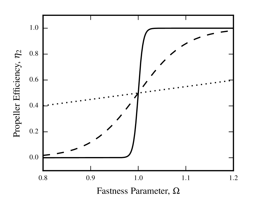
Refer to caption
Figure 1: A demonstration of how quickly the propeller switches on as a function of n𝑛n described by Equation (10). The dotted line corresponds to n=1𝑛1n=1, the dashed line corresponds to n=10𝑛10n=10, and the solid line corresponds to n=100𝑛100n=100.

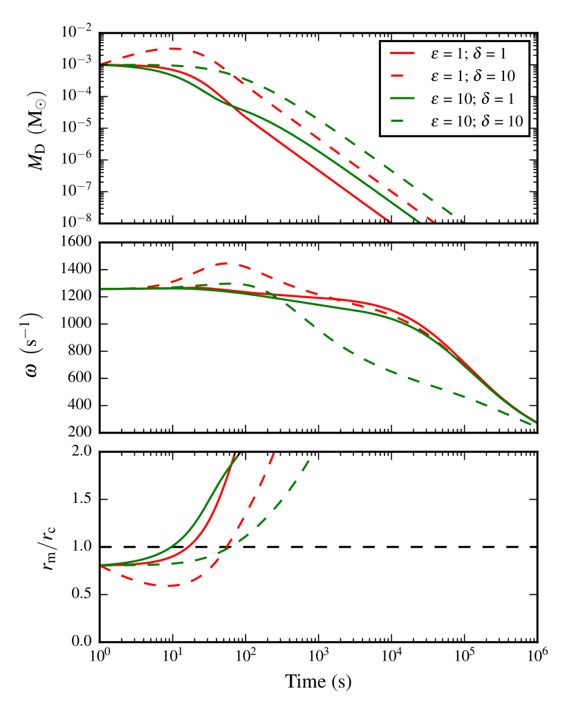
We parameterise the available fallback mass as a fraction (δ𝛿\delta) of the initial disc mass, Mfb=δMD,isubscript𝑀fb𝛿subscript𝑀DiM_{\rm fb}=\delta M_{\rm D,i}, and the fallback timescale is similarly parameterised as a fraction (ϵitalic-ϵ\epsilon) of the viscous timescale, tfb=ϵtνsubscript𝑡fbitalic-ϵsubscript𝑡𝜈t_{\rm fb}=\epsilon t_{\rm\nu}. Equations (3) and (4) are coupled, first order, ordinary differential equations (ODEs) and, using an ODE integrator, the values of MDsubscript𝑀DM_{\rm D} and ω𝜔\omega can be calculated for a given range of time points. Fig. 2 demonstrates how these fallback parameters affect the disc mass and rotational frequency of a magnetar and disc system and how the propeller condition rm/rcsubscript𝑟msubscript𝑟cr_{\rm m}/r_{\rm c} evolves with time.

Refer to caption
Figure 2: A demonstration of how different combinations of the fallback parameters ϵitalic-ϵ\epsilon and δ𝛿\delta affect the disc mass (top panel) and rotation frequency (centre panel) of a magnetar and disc system with fixed magnetic field, initial spin period, initial disc mass and radius. The bottom panel shows the evolution of the propeller condition rm/rcsubscript𝑟msubscript𝑟cr_{\rm m}/r_{\rm c} over time for each combination. The system is in the propeller regime when rm/rc>1subscript𝑟msubscript𝑟c1r_{\rm m}/r_{\rm c}>1 (i.e. above the black, dashed line).

For short timescales and small fallback masses (ϵ=1italic-ϵ1\epsilon=1; δ=1𝛿1\delta=1; solid, red curve), the magnetar spins up more slowly despite rapid fallback because the disc is only being fed small amounts of mass. Hence, the propeller mechanism turns on earlier since the propeller condition is at a lower frequency. For short timescales and large fallback masses (ϵ=1italic-ϵ1\epsilon=1; δ=10𝛿10\delta=10; dashed, red curve), mass is quickly added to the disc and the magnetar spins up rapidly. The propeller mechanism is turned on later because the conditional frequency is higher. For long timescales and small fallback masses (ϵ=10italic-ϵ10\epsilon=10; δ=1𝛿1\delta=1; solid, green curve), the disc is fed a small amount of mass very slowly and so the magnetar spins up gradually. Again, the propeller condition is at a lower frequency and, therefore, the mechanism turns on earlier. For long timescales and large fallback masses (ϵ=10italic-ϵ10\epsilon=10; δ=10𝛿10\delta=10; dashed, green curve), the disc mass stays constant over a longer period providing a gentle spin-up of the magnetar. Again, the propeller condition is a higher frequency and the mechanism turns on later. Generally speaking, an initially denser disc makes the propeller mechanism harder to initiate, but the magnetar is spun up more rapidly and, therefore, satisfies the propeller condition at an earlier time.

Once Equations (3) and (4) have been integrated, they are then used to estimate the luminosities from the dipole and propelled components, such that

Lprop=ηprop[Naccω(η2GMMDrmtν)]subscript𝐿propsubscript𝜂propdelimited-[]subscript𝑁acc𝜔subscript𝜂2𝐺𝑀subscript𝑀Dsubscript𝑟msubscript𝑡𝜈L_{\rm prop}=\eta_{\rm prop}\Bigg{[}-N_{\rm acc}\omega-\left(\eta_{\rm 2}\frac{GMM_{\rm D}}{r_{\rm m}t_{\rm\nu}}\right)\Bigg{]} (11)

and

Ldip=ηdipμ2ω46c3,subscript𝐿dipsubscript𝜂dipsuperscript𝜇2superscript𝜔46superscript𝑐3L_{\rm dip}=\eta_{\rm dip}\frac{\mu^{2}\omega^{4}}{6c^{3}}, (12)

where ηpropsubscript𝜂prop\eta_{\rm prop} and ηdipsubscript𝜂dip\eta_{\rm dip} are the propeller and dipole energy-luminosity conversion efficiencies respectively. The total luminosity is given by the sum of the dipole and propeller luminosities and divided by a beaming fraction to account for the relativistic beaming of the jet: Ltot=(1/fB)(Ldip+Lprop)subscript𝐿tot1subscript𝑓Bsubscript𝐿dipsubscript𝐿propL_{\rm tot}=\left(1/f_{\rm B}\right)\left(L_{\rm dip}+L_{\rm prop}\right). 1/fB1subscript𝑓B1/f_{\rm B} is the fraction of the stellar sphere which is emitting and is related to the half-opening angle of the jet, θjsubscript𝜃j\theta_{\rm j}, as: 1/fB=1cos(θj)1subscript𝑓B1subscript𝜃j1/f_{\rm B}=1-\cos(\theta_{\rm j}) (Rhoads, 1999; Sari et al., 1999).

2.1 Comparing dipole torque equations

For the dipole torque, we have used the classical solution as given by Shapiro & Teukolsky (1983) and Piro & Ott (2011).

Ndip=μ2ω36c3.subscript𝑁dipsuperscript𝜇2superscript𝜔36superscript𝑐3N_{\rm dip}=-\frac{\mu^{2}\omega^{3}}{6c^{3}}. (13)

The negative sign indicates that Ndipsubscript𝑁dipN_{\rm dip} spins the magnetar down and produces dipole emission. However, work done by Gompertz et al. (2014) instead uses the following form for the dipole torque

Ndip=23μ2ω3c3(rlcrm)3,subscript𝑁dip23superscript𝜇2superscript𝜔3superscript𝑐3superscriptsubscript𝑟lcsubscript𝑟m3N_{\rm dip}=-\frac{2}{3}\frac{\mu^{2}\omega^{3}}{c^{3}}{\left(\frac{r_{\rm lc}}{r_{\rm m}}\right)}^{3}, (14)

which is Equation (2)2(2) in Bucciantini et al. (2006).

Bucciantini et al. (2006) use a relativistic magneto-hydrodynamic (MHD) treatment to solve for the plasma winds emanating from a rotating NS and accretion disc system. They assume that the flow emerges from open flux tubes (providing the extent and shape of the open field line region in the magnetic field is known) and that a truncation of the disc produces more open flux tubes and, therefore, a greater mass loss. Equation (14) is then derived from these assumptions. However, it is not certain that these assumptions apply within the model presented in this work and a full MHD treatment of the magnetic propeller is not presented. Therefore, Equation (13) is used rather than introduce uncertain assumptions into the model. A comparison between Equations (13) and (14) is shown in Fig. 3 using a synthetic GRB light curve with arbitrary parameters.
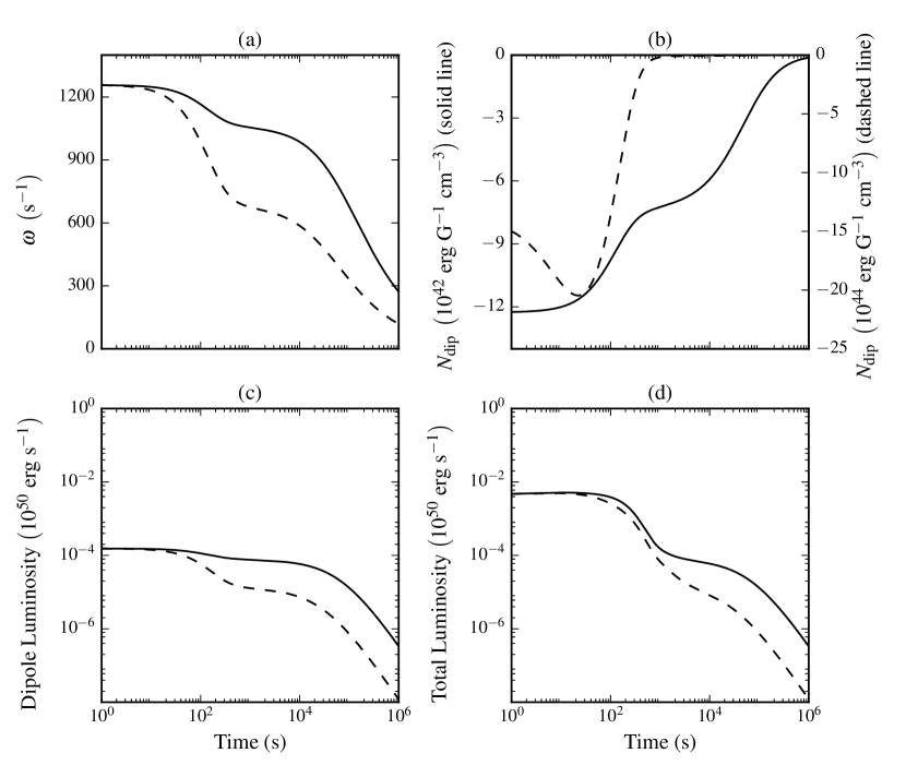
Refer to caption
Figure 3: A comparison of how Equation (13) (solid line; Piro & Ott 2011) and Equation (14) (dashed line; Bucciantini et al. 2006) affect (a) the stellar spin; (b) the dipole torque; (c) the dipole luminosity; and (d) the total luminosity of a synthetic GRB light curve.

2.2 Exploring parameter space

Table 1: Values used to test the effect of parameter variation on the shape of a GRB light curve. B𝐵B - magnetic field; Pisubscript𝑃iP_{\rm i} - initial spin period; MD,isubscript𝑀DiM_{\rm D,i} - initial disc mass; RDsubscript𝑅DR_{\rm D} - disc radius; ϵitalic-ϵ\epsilon - timescale ratio; δ𝛿\delta - fraction of initial disc mass available in the global mass budget; n𝑛n - sharpness of propeller switch-on.
B𝐵B (1015superscript101510^{15} G) 111 555 101010 505050 -
Pisubscript𝑃iP_{\rm i} (ms) 111 555 101010 - -
MD,isubscript𝑀DiM_{\rm D,i} (M)subscript𝑀direct-product\left(M_{\rm\odot}\right) 105superscript10510^{-5} 104superscript10410^{-4} 103superscript10310^{-3} 102superscript10210^{-2} 101superscript10110^{-1}
RDsubscript𝑅DR_{\rm D} (km) 100100100 500500500 100010001000 - -
ϵitalic-ϵ\epsilon 111 101010 - - -
δ𝛿\delta 111 101010 - - -
n𝑛n 111 101010 505050 - -

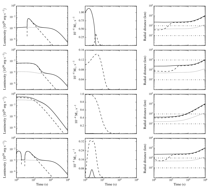
To determine how the modifications to the propeller model have affected the phenomenological classes outlined in Gompertz et al. (2014) (humped, classic, sloped and stuttering), the parameter variation experiment they originally performed was repeated with values from Table 1. The magnetar mass and radius were fixed to be 1.4M1.4subscript𝑀direct-product1.4~{}M_{\rm\odot} and 101010 km respectively, the propeller and dipole efficiencies were set to 100%percent100100\% and the the beaming fraction to 111 since they only act to normalise the luminosity here. The produced light curves represented all combinations of B𝐵B, Pisubscript𝑃iP_{\rm i}, MD,isubscript𝑀DiM_{\rm D,i}, RDsubscript𝑅DR_{\rm D}, ϵitalic-ϵ\epsilon, δ𝛿\delta, and n𝑛n. The four phenomenological types originally outlined in Gompertz et al. (2014) were recovered and examples of each are shown in Fig. 4. All values for n𝑛n appeared commonly in each type suggesting that the model is insensitive to n𝑛n.

Refer to caption
Figure 4: Top to bottom: Type I - Humped; Type II - Classic; Type III - Sloped; Type IV - Stuttering. Each row shows plots for one example of each class. They are not fully representative of the range of energetics or morphology for their respective classes since they are intended to highlight the light curve shapes only. Left panels: synthetic light curves representing the four phenomenological classes. Dotted line - dipole luminosity; dashed line - propeller luminosity; solid line - total luminosity. Centre panels: mass flow rates in the system. Solid line - mass flow rate on to the central magnetar; dashed line - propellered mass flow out of the system. Right panels: positions of key radii relative to the centre of the magnetar. Dashed line - Alfvén radius; dotted line - co-rotation radius; solid line - light cylinder radius. Lower horizontal dot-dashed line is the magnetar radius, upper horizontal dot-dashed line is the outer disc radius, RDsubscript𝑅DR_{\rm D}.

2.3 Comparing types to previous work

Table 2: Main parameters used to compare light curves from the previous model (Gompertz et al. 2014) with the modified model without fallback accretion.
Humped Classic Sloped Stuttering
B𝐵B (1015superscript101510^{15} G) 111 111 101010 555
Pisubscript𝑃iP_{\rm i} (ms) 555 555 555 555
MD,isubscript𝑀DiM_{\rm D,i} (M)subscript𝑀direct-product\left(M_{\rm\odot}\right) 103superscript10310^{-3} 104superscript10410^{-4} 104superscript10410^{-4} 102superscript10210^{-2}
RDsubscript𝑅DR_{\rm D} (km) 100100100 100010001000 100010001000 500500500

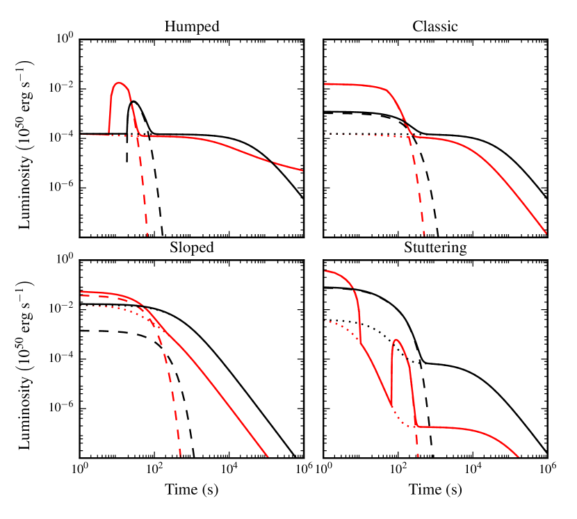
In order to determine how well the modified model recovered the four types, the parameters given in Table 2 were used to generate light curves using the previous model described in Gompertz et al. (2014). The fallback accretion in the modified model was turned off by setting ϵ=1italic-ϵ1\epsilon=1 and δ=106𝛿superscript106\delta=10^{-6}, i.e. the amount of fallback mass is so negligible that the magnetar behaves as if only the accretion disc is present and the fallback timescale becomes irrelevant. The value of n𝑛n used was 111 as this is the closest approximation to the propeller switch-on modelled in previous work. Fig. 5 compares the modified model without fallback to the previous work. The difference in dipole luminosity between the two models is explained by our use of the classical dipole torque as discussed in Section 2.1. Equation (13) has a longer dipole duration than Equation (14) causing some morphological differences. However, the modified model does not recover the propeller luminosity in all cases, the stuttering type being the most different. Since we have already seen in Fig. 4 that the modified model is capable of reproducing all types successfully, it is suggested that they have moved in parameter space due to the inclusion of M˙propsubscript˙𝑀prop\dot{M}_{\rm prop} and it’s link to M˙accsubscript˙𝑀acc\dot{M}_{\rm acc} through η2subscript𝜂2\eta_{\rm 2}.

Refer to caption
Figure 5: Comparison of light curves generated by the previous model (Gompertz et al. 2014; red curves) and the modified model without fallback accretion (black curves). The fallback was turned off by setting ϵ=1italic-ϵ1\epsilon=1 and δ=106𝛿superscript106\delta=10^{-6}; n=1𝑛1n=1 as the closest approximation to the switch on in the previous model. Solid lines - total luminosity; dashed lines - propeller luminosity; dotted lines - dipole luminosity.

3 Swift SGRBEE Sample

The data for the GRB sample were collected by Swift. The Swift satellite (Gehrels et al., 2004), launched in 2004, is a multi-wavelength observatory dedicated to GRB hunting with rapid slewing capabilities. It carries three instruments: the Burst Alert Telescope (BAT; Barthelmy et al. 2005), the X-ray Telescope (XRT; Burrows et al. 2005), and the Ultra-Violet/Optical Telescope (UVOT; Roming et al. 2005). The Swift mission and the UK Swift Science Data Centre (UKSSDC111www.swift.ac.uk, Evans et al. 2007, 2009) provided the data presented in this paper.

The data need to undergo a cosmological k𝑘k-correction and absorption correction, as described in Bloom et al. (2001), to produce bolometric (1 - 10000 keV), redshift-corrected light curves before they can be fitted by the model. This method requires the photon index, ΓΓ\Gamma, the absorption coefficient, σ𝜎\sigma (given by the ratio of counts-to-flux unabsorbed to counts-to-flux observed, which are all available on the UKSDCC repository) and the redshift, z𝑧z, some of which were found in the literature (see Table 3). For those GRBs with no measured redshift, the sample mean of 0.390.390.39 from Gompertz et al. (2014) was used. Alternatively, a randomly generated redshift (e.g. within 1,2121,~{}2 or even 333 standard deviations of the mean value) could be used. The effect of an increasing z𝑧z is an increase in luminosity and earlier on-set times that, as we will see later in this paper, causes the model to favour larger initial disc masses and fallback mass budgets. Since these may not have a physical basis, we have chosen to use the sample mean, as in previous work by Gompertz et al. (2014).

Table 3: The sample of SGRBEEs and the parameters required for a cosmological k𝑘k-correction. For GRBs with an unknown redshift (marked with an ), the sample mean of 0.390.390.39 from Gompertz et al. (2014) was used. Upper limit (D’Avanzo et al., 2009). aProchaska et al. (2005); bSoderberg et al. (2005); cPrice et al. (2006); cBerger (2007); dCenko et al. (2006); eGraham et al. (2009); fD’Avanzo et al. (2007); gSelsing et al. (2016).
GRB ΓΓ\Gamma σ𝜎\sigma z𝑧z
050724 1.580.19+0.21subscriptsuperscript1.580.210.191.58^{+0.21}_{-0.19} 1.261.261.26 0.2578asuperscript0.2578a0.2578^{\rm a}
051016B 1.850.13+0.14subscriptsuperscript1.850.140.131.85^{+0.14}_{-0.13} 1.311.311.31 0.9364bsuperscript0.9364b0.9364^{\rm b}
051227 2.10.4+0.4subscriptsuperscript2.10.40.42.1^{+0.4}_{-0.4} 1.311.311.31 2.8superscript2.82.8^{\dagger}
060614 1.780.08+0.08subscriptsuperscript1.780.080.081.78^{+0.08}_{-0.08} 1.061.061.06 0.1254csuperscript0.1254c0.1254^{\rm c}
061006 2.10.4+0.6subscriptsuperscript2.10.60.42.1^{+0.6}_{-0.4} 1.611.611.61 0.4377csuperscript0.4377c0.4377^{\rm c}
061210 2.600.71+1.92subscriptsuperscript2.601.920.712.60^{+1.92}_{-0.71} 3.483.483.48 0.4095dsuperscript0.4095d0.4095^{\rm d}
070714B 1.790.22+0.24subscriptsuperscript1.790.240.221.79^{+0.24}_{-0.22} 1.151.151.15 0.9224esuperscript0.9224e0.9224^{\rm e}
071227 1.50.5+0.6subscriptsuperscript1.50.60.51.5^{+0.6}_{-0.5} 1.021.021.02 0.381fsuperscript0.381f0.381^{\rm f}
080123 2.460.70+1.04subscriptsuperscript2.461.040.702.46^{+1.04}_{-0.70} 1.711.711.71 0.39superscript0.390.39^{*}
080503 2.380.16+0.42subscriptsuperscript2.380.420.162.38^{+0.42}_{-0.16} 1.241.241.24 0.39superscript0.390.39^{*}
100212A 1.990.18+0.40subscriptsuperscript1.990.400.181.99^{+0.40}_{-0.18} 1.371.371.37 0.39superscript0.390.39^{*}
100522A 2.400.16+0.17subscriptsuperscript2.400.170.162.40^{+0.17}_{-0.16} 2.452.452.45 0.39superscript0.390.39^{*}
111121A 1.780.20+0.21subscriptsuperscript1.780.210.201.78^{+0.21}_{-0.20} 1.421.421.42 0.39superscript0.390.39^{*}
150424A 1.980.22+0.24subscriptsuperscript1.980.240.221.98^{+0.24}_{-0.22} 1.231.231.23 0.39superscript0.390.39^{*}
160410A 1.50.6+0.7subscriptsuperscript1.50.70.61.5^{+0.7}_{-0.6} 1.021.021.02 1.717gsuperscript1.717g1.717^{\rm g}

The sample studied in Gompertz et al. (2013) and Gompertz et al. (2014) has been expanded here by selecting identified SGRBEEs from Kaneko et al. (2015) (which covers bursts to the end of 2012) that have good data available in the Swift archive. Plus GRBs 150424A and 160410A which are identified as EE bursts within GCN Circulars (Norris et al. 2015 and Sakamoto et al. 2016 respectively). The data used in the fitting incorporates XRT data and BAT data that have been extrapolated into the XRT bandpass (available from the UKSDCC Burst Analyser tool) since the effect of the extended emission is not always evident in the XRT light curve alone.

4 Fitting Routine

A Markov chain Monte Carlo simulation (MCMC; MacKay 2003, chap. 4) was used to fit the model to data as there are a minimum of six parameters and the MCMC will efficiently search a large portion of parameter space and increase the probability of finding the global minimum of the model. However, the MCMC method requires a burn-in phase which is loosely defined as an unknown number of steps at the beginning of the simulation where each “walker” attempts to find the lowest area of probability space. The chain is generally considered to be burned in when all walkers have converged onto this area of probability space. The “emcee” module was used to handle the MCMC (Foreman-Mackey et al., 2013). To construct the posterior probability distribution, a Gaussian log-likelihood function of the following form was chosen

ln(plikelihood)=12i=1N(yiy^iσi)2,subscript𝑝likelihood12superscriptsubscript𝑖1𝑁superscriptsubscript𝑦𝑖subscript^𝑦𝑖subscript𝜎𝑖2\ln(p_{\rm likelihood})=-\frac{1}{2}\sum_{i=1}^{N}{\left(\frac{y_{i}-\hat{y}_{i}}{\sigma_{i}}\right)}^{2}, (15)

where yisubscript𝑦𝑖y_{i} is a data point, σisubscript𝜎𝑖\sigma_{i} is it’s associated uncertainty, and y^isubscript^𝑦𝑖\hat{y}_{i} is a model point calculated at the same x𝑥x-value as yisubscript𝑦𝑖y_{i}. The Swift light curves used here are binned to contain a minimum of 202020 photons per time bin (an exception may be applicable in the last bin) making Gaussian statistics suitable. A prior probability that is flat when the parameters are within the limits given in Table 4 was also chosen.

ln(pprior)={0:xl<x<xu:otherwisesubscript𝑝priorcases0:absentsubscript𝑥𝑙𝑥subscript𝑥𝑢:absent𝑜𝑡𝑒𝑟𝑤𝑖𝑠𝑒\ln(p_{\rm prior})=\left\{\begin{array}[]{lr}~{}0&:x_{l}<x<x_{u}\\ -\infty&:otherwise\end{array}\right. (16)

Hence, the full posterior probability distribution is given by

ln(p)=ln(plikelihood)+ln(pprior).𝑝subscript𝑝likelihoodsubscript𝑝prior\ln(p)=\ln(p_{\rm likelihood})+\ln(p_{\rm prior}). (17)
Table 4: Upper and lower limits placed on the fitting parameters in the MCMC. MD,isubscript𝑀DiM_{\rm D,i}, RDsubscript𝑅DR_{\rm D}, ϵitalic-ϵ\epsilon, and δ𝛿\delta were searched in log-space for efficiency.
Lower Upper
B𝐵B (1015superscript101510^{15} G) 103superscript10310^{-3} 101010
Pisubscript𝑃iP_{\rm i} (ms) 0.690.690.69 101010
MD,isubscript𝑀DiM_{\rm D,i} (Msubscript𝑀direct-productM_{\rm\odot}) 103superscript10310^{-3} 101superscript10110^{-1}
RDsubscript𝑅DR_{\rm D} (km) 505050 200020002000
ϵitalic-ϵ\epsilon 0.10.10.1 100010001000
δ𝛿\delta 105superscript10510^{-5} 505050
ηdipsubscript𝜂dip\eta_{\rm dip} (%) 111 100100100
ηpropsubscript𝜂prop\eta_{\rm prop} (%) 111 100100100
1/fB1subscript𝑓B1/f_{\rm B} 111 600600600

For the MCMC, 100100100 affine invariant walkers (Goodman & Weare, 2010) were used and ran for a 50,0005000050,000 step burn in phase to allow the walkers to test all of parameter space. After this run, the best 100100100 distinct probabilities were chosen to serve as the starting point for the final MCMC run of the same length. This made sure that the parameters recovered were representative of the global minimum, not a local minimum, and reduces the burn-in of the chain to 1000less-than-or-similar-toabsent1000\lesssim 1000 steps in most cases. Although, if the time series (parameter or probability value vs. model number for each walker) showed that the chain had not fully converged, the process of selecting the 100100100 best probabilities was repeated and the chain run again until convergence was achieved. The optimal parameters were found by taking the median of the posterior probability distributions and their uncertainties are given by the 95%percent9595\% percentiles. We chose the median, rather than the mean or mode, since it is less sensitive to the tails of distributions and is preserved under reversible transformations of the data (e.g. log10ϵϵsubscript10italic-ϵitalic-ϵ\log_{10}\epsilon\rightarrow\epsilon). Fits for the SGRBEE sample were produced with a range of free parameters (p)𝑝(p): p=6𝑝6p=6 (B𝐵B, Pisubscript𝑃iP_{\rm i}, MD,isubscript𝑀DiM_{\rm D,i}, RDsubscript𝑅DR_{\rm D}, ϵitalic-ϵ\epsilon and δ𝛿\delta); 777 (original 666 plus 1/fB1subscript𝑓B1/f_{\rm B}); 888 (original 666 plus ηdipsubscript𝜂dip\eta_{\rm dip} and ηpropsubscript𝜂prop\eta_{\rm prop}); and 999 (all listed parameters). ηdipsubscript𝜂dip\eta_{\rm dip}, ηpropsubscript𝜂prop\eta_{\rm prop} and 1/fB1subscript𝑓B1/f_{\rm B} were fixed to 5%percent55\%, 40%percent4040\% and 111 respectively when they were not free parameters, in keeping with Gompertz et al. (2014). The fits were repeated for fixed values of n=1,10,100𝑛110100n=1,~{}10,~{}100 and the corrected Akaike Information Criterion (AICc; Cavanaugh & Neath 2011) was used to establish the best fitting models. We chose this statistic since it allows us to compare models of varying free parameter number (p𝑝p).

AICc is given by the following equation

AICc=2ln(L)+2k+2k(k+1)Nk1,𝐴𝐼𝐶𝑐2𝐿2𝑘2𝑘𝑘1𝑁𝑘1AICc=-2\ln(L)+2k+\frac{2k(k+1)}{N-k-1}, (18)

where k𝑘k is the number of free parameters and N𝑁N is the number of observations in the data set. This penalises a model for ‘overfitting’ and scales with k𝑘k. We have substituted Equation (15) for the maximum log-likelihood ln(L)𝐿\ln(L), which then cancels down to the χ2superscript𝜒2\chi^{2} statistic. The minimum AICc value within a set is then representative of the optimum model fit since if the AICc value of a model that has a large number of free parameters (and hence a large penalty) is less than a model with fewer free parameters (and hence a small penalty), then it can be generally assumed that the extra parameters improve the quality of fit.

5 Results and Discussion

Table 5: AICc values for models using 666, 777, 888 and 999 free parameters (p𝑝p) for n=1,10,100𝑛110100n=1,10,100. Underlined values are the lowest AICc values for each n𝑛n bracket and values in bold are the minima across all values of n𝑛n. Values marked with an are modified since Nk1=0𝑁𝑘10N-k-1=0 for these models.
n=1𝑛1n=1 n=10𝑛10n=10 n=100𝑛100n=100
GRB p=6𝑝6p=6 p=7𝑝7p=7 p=8𝑝8p=8 p=9𝑝9p=9 p=6𝑝6p=6 p=7𝑝7p=7 p=8𝑝8p=8 p=9𝑝9p=9 p=6𝑝6p=6 p=7𝑝7p=7 p=8𝑝8p=8 p=9𝑝9p=9
050724 2,41524152,415 1,79017901,790 1,97519751,975 1,682¯¯1682\underline{1,682} 2,49624962,496 2,21622162,216 2,00520052,005 𝟏,𝟓𝟎𝟕15071,507 2,50925092,509 2,12821282,128 2,00720072,007 1,610¯¯1610\underline{1,610}
051016B 802802802 540540540 771771771 531¯¯531\underline{531} 785785785 562562562 742742742 518¯¯518\underline{518} 785785785 549549549 742742742 𝟒𝟑𝟓435435
051227 538538538 267267267 318318318 235¯¯235\underline{235} 535535535 271271271 317317317 235¯¯235\underline{235} 535535535 381381381 317317317 𝟐𝟑𝟑233233
060614 47,3904739047,390 47,2564725647,256 47,5214752147,521 𝟒𝟒,𝟕𝟎𝟗4470944,709 48,4284842848,428 47,2754727547,275 46,9504695046,950 44,746¯¯44746\underline{44,746} 48,4224842248,422 47,2634726347,263 48,0134801348,013 45,278¯¯45278\underline{45,278}
061006 269269269 244¯¯244\underline{244} 252252252 250250250 317317317 𝟐𝟒𝟐242242 543543543 253253253 323323323 244¯¯244\underline{244} 262262262 257257257
061210 673¯¯673\underline{673} 802802802 1,0541superscript0541,054^{*} 103,101103101103,101 677677677 𝟏𝟒𝟗149149 1,6491superscript6491,649^{*} 5,14851485,148 670670670 210¯¯210\underline{210} 969superscript969969^{*} 5,12751275,127
070714B 1,30313031,303 1,41914191,419 1,260¯¯1260\underline{1,260} 1,35213521,352 1,30213021,302 1,39713971,397 1,260¯¯1260\underline{1,260} 1,30113011,301 1,30213021,302 1,84418441,844 1,26012601,260 𝟏,𝟏𝟖𝟎11801,180
071227 335335335 161161161 163163163 𝟏𝟓𝟖158158 226226226 339339339 161¯¯161\underline{161} 163163163 225225225 265265265 161¯¯161\underline{161} 230230230
080123 308308308 308308308 298¯¯298\underline{298} 305305305 337337337 291¯¯291\underline{291} 308308308 307307307 360360360 𝟐𝟖𝟑283283 330330330 360360360
080503 2,335¯¯2335\underline{2,335} 2,37523752,375 2,47424742,474 2,47424742,474 2,37523752,375 2,37923792,379 𝟐,𝟐𝟗𝟒22942,294 2,58325832,583 2,92729272,927 2,475¯¯2475\underline{2,475} 3,53935393,539 2,78427842,784
100212A 9,05590559,055 8,37283728,372 8,13081308,130 𝟕,𝟑𝟏𝟎73107,310 9,29992999,299 8,27182718,271 8,98889888,988 8,196¯¯8196\underline{8,196} 9,25892589,258 8,498¯¯8498\underline{8,498} 8,98889888,988 8,58885888,588
100522A 29,3772937729,377 22,992¯¯22992\underline{22,992} 27,4722747227,472 23,4192341923,419 27,6662766627,666 23,3262332623,326 26,1162611626,116 𝟐𝟐,𝟏𝟖𝟒2218422,184 27,5312753127,531 22,4602246022,460 26,7442674426,744 22,411¯¯22411\underline{22,411}
111121A 1,75417541,754 1,747¯¯1747\underline{1,747} 1,76117611,761 1,80318031,803 1,75317531,753 1,75117511,751 1,748¯¯1748\underline{1,748} 1,76617661,766 1,75317531,753 1,75017501,750 1,76117611,761 𝟏,𝟕𝟒𝟐17421,742
150424A 2,37723772,377 2,99729972,997 2,22322232,223 𝟏,𝟑𝟑𝟒13341,334 2,31523152,315 51,2465124651,246 2,170¯¯2170\underline{2,170} 58,0805808058,080 2,31523152,315 1,79517951,795 2,17121712,171 1,432¯¯1432\underline{1,432}
160410A 974974974 473¯¯473\underline{473} 546546546 18,7421874218,742 1,11511151,115 366¯¯366\underline{366} 546546546 403403403 1,25512551,255 412412412 546546546 𝟑𝟓𝟗359359

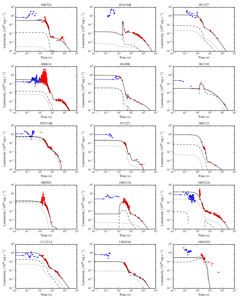
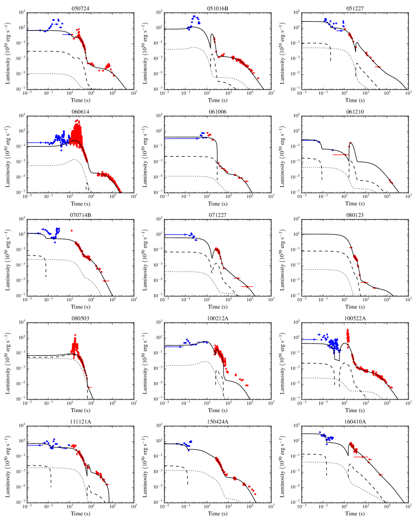
Table 5 presents the AICc values for all results of the fitting routine. The large spread of values is representative of the difficulty χ2superscript𝜒2\chi^{2} (the root of the AICc) has comparing a smooth model with highly variable data, especially in the early-time BAT data. Table 5 shows that the general picture of the model is stable over all n𝑛n values since there is a reasonable spread of best fits. This also confirms the observation made in Section 2.2 that the model is reasonably insensitive to n𝑛n. Increasing n𝑛n only makes features such as humps appear sharper, which does not have a great impact on the overall quality of the fit. The best global fits to the SGRBEE sample (bold values in Table 5) are presented in Fig. 6.
Refer to caption
Figure 6: Best global fits to the SGRBEE sample (bold values in Table 5). Dashed line - propeller luminosity; dotted line - dipole luminosity; solid line - total luminosity; red points - combined BAT and XRT data.

The p=6𝑝6p=6 set represents the core physics of the model by constraining the fundamental properties of the magnetar (B𝐵B and Pisubscript𝑃iP_{\rm i}), the accretion disc (MD,isubscript𝑀DiM_{\rm D,i} and RDsubscript𝑅DR_{\rm D}) and the fallback (Mfbsubscript𝑀fbM_{\rm fb} and tfbsubscript𝑡fbt_{\rm fb} through δ𝛿\delta and ϵitalic-ϵ\epsilon respectively) and is the most energetically restricted case compared to the p=9𝑝9p=9 case which has the largest energy reservoir. Furthermore, ηdipsubscript𝜂dip\eta_{\rm dip} and ηpropsubscript𝜂prop\eta_{\rm prop} determine the efficiency at which the dipole and propeller mechanisms respectively need to work at in order to convert the energy to luminosity. Lastly, fBsubscript𝑓Bf_{\rm B} accounts the anisotropy of the radiation (1/fB1subscript𝑓B1/f_{\rm B} is the solid angle of emission). The results of the MCMC were analysed for parameter correlations though none were found since our method of selecting the best probabilities after the burn-in phase removes any correlation by placing the parameters in the global minimum.

The k𝑘k-correction performed in Section 3 assumes isotropic emission, whereas in actuality, GRBs are beamed into a very narrow opening angle due to their relativistic velocity (Fruchter et al., 1999; Harrison et al., 1999; Frail et al., 2001). Rather than divide the data down to a beam-corrected level, our routine works to multiply the model up to the isotropic luminosity level so that model comparison becomes easier on the same scale. The morphologies of the fits change as each new parameter is introduced since they handle the high luminosities at early times allowing the core parameters to reconfigure. This means that there can be more energy available at late times to fit the fading afterglow.

It is interesting to compare the freedom of the model (i.e. how many free parameters are used) with the “sharpness” of the propeller (i.e. the n𝑛n value). Generally speaking, the AICc value of the fit improves as the number of free parameters increases, whereas, increasing n𝑛n for the same number of free parameters often does not improve the fit. Also, p=8𝑝8p=8 fits often perform worse than p=7𝑝7p=7 fits implying that the beaming fraction has a greater role within the model than the efficiencies, but the inclusion of all 333 of these parameters are most preferable. Table 6 shows a comparison of the jet half-opening angles derived from the best fits in this work with hydrodynamical modelling performed by Ryan et al. (2015) for 444 GRBs common to both studies. Our model produces systematically narrower jets (most likely caused by the models attempts to fit the early-time luminosity) which are partially consistent with Ryan et al. (2015) in errors (e.g. GRBs 051016B and 060614), and where they are not (e.g. GRB 061006), they are broadly consistent to 22.5σsimilar-toabsent22.5𝜎\sim 2-2.5\sigma.

Table 6: Table showing the half-opening angles (in radians) for 444 GRBs, calculated from fB=1cos(θj)subscript𝑓B1subscript𝜃jf_{\rm B}=1-\cos\left(\theta_{\rm j}\right). θjsubscript𝜃j\theta_{\rm j} values are from the global best fits of this work (uncertainties are 95%percent9595\% confidence interval); θ0subscript𝜃0\theta_{\rm 0} values are from Ryan et al. (2015).
GRB θjsubscript𝜃j\theta_{\rm j} θ0subscript𝜃0\theta_{\rm 0}
051016B 0.070.11+0.11subscriptsuperscript0.070.110.110.07^{+0.11}_{-0.11} 0.350.24+0.11subscriptsuperscript0.350.110.240.35^{+0.11}_{-0.24}
060614 0.0790.500+0.359subscriptsuperscript0.0790.3590.5000.079^{+0.359}_{-0.500} 0.2930.085+0.122subscriptsuperscript0.2930.1220.0850.293^{+0.122}_{-0.085}
061006 0.0780.081+0.088subscriptsuperscript0.0780.0880.0810.078^{+0.088}_{-0.081} 0.4070.173+0.068subscriptsuperscript0.4070.0680.1730.407^{+0.068}_{-0.173}
070714B 0.060.12+0.18subscriptsuperscript0.060.180.120.06^{+0.18}_{-0.12} 0.330.11+0.11subscriptsuperscript0.330.110.110.33^{+0.11}_{-0.11}

Comparing our results with that of Gompertz et al. (2014), we can see the inclusion of fallback accretion within the propeller model allows for an improvement in fitting the ‘tail’ of the fading afterglow. This is can be seen in GRBs 051227, 060614 and 061006 where Gompertz et al. (2014) did not produce such good fits to the tail. Hence, fallback accretion is a necessary addition to the propeller model in order to fully explain the energetics and morphologies of SGRBEEs. Additionally, the extended model handles variability and flares within the data much more naturally than Gompertz et al. (2014) and copes with the early-time luminosity detected by BAT.

The parameters derived from the fits in Fig. 6 are presented in Table 7. We find that the magnetic fields derived from the fits are in the moderate to high end of the parameter space and that the sample generally have slow initial spins. The slow initial spins are most likely due to the additional fallback spinning the magnetar up and, therefore, the constraints on high initial spin rates is relaxed. This has an impact on the value of the magnetic field derived as the fit moves along the correlation between B𝐵B and Pisubscript𝑃iP_{\rm i} discussed in Gompertz et al. (2014). The sample fits also tend to favour massive discs and narrow jet opening angles. This is most likely due to the model extracting as much of the available energy as possible to fit the high luminosities at early times in the light curve, data which was not included in the fits of Gompertz et al. (2014). The values of ϵitalic-ϵ\epsilon, δ𝛿\delta, ηdipsubscript𝜂dip\eta_{\rm dip} and ηpropsubscript𝜂prop\eta_{\rm prop} are widely distributed throughout the parameter space. The derived parameters are consistent with predictions for a magnetar (Giacomazzo & Perna 2013; Mereghetti et al. 2015; Rea et al. 2015) and are also consistent with the results in Gompertz et al. (2014).

We will now examine how increasing the number of free parameters affects the fits in 333 GRBs from the sample. GRB 060614 has been chosen since this is a uniquely interesting burst given its characteristics. GRBs 050724 and 111121A were chosen as examples of the model behaving consistently well, or vice versa, over the different parameter sets.

Table 7: Parameters derived from the best global fits to the SGRBEE sample (bold values in Table 5). Reported errors are 95%percent9595\%. Values marked with an [L] have reached a parameter limit; those marked with [F] were fixed during fitting. The χred2subscriptsuperscript𝜒2red\chi^{2}_{\rm red} values are also presented to indicate goodness of fit.
GRB n𝑛n[F] B𝐵B Pisubscript𝑃iP_{\rm i} MD,isubscript𝑀DiM_{\rm D,i} RDsubscript𝑅DR_{\rm D} ϵitalic-ϵ\epsilon δ𝛿\delta ηdipsubscript𝜂dip\eta_{\rm dip} ηpropsubscript𝜂prop\eta_{\rm prop} 1/fB1subscript𝑓B1/f_{\rm B} χred2subscriptsuperscript𝜒2red\chi^{2}_{\rm red}
(×1015absentsuperscript1015\times 10^{15} G) (ms) (×102M)\left(\times 10^{-2}~{}M_{\rm\odot}\right) (km) (%) (%)
050724 101010 4.810.23+0.11subscriptsuperscript4.810.110.234.81^{+0.11}_{-0.23} 9.700.92+0.29subscriptsuperscript9.700.290.929.70^{+0.29}_{-0.92} 0.4890.023+0.070subscriptsuperscript0.4890.0700.0230.489^{+0.070}_{-0.023} 3205+5subscriptsuperscript32055320^{+5}_{-5} 1.261.15+11.87subscriptsuperscript1.2611.871.151.26^{+11.87}_{-1.15} (0.500.30+1.82)×103subscriptsuperscript0.501.820.30superscript103\left(0.50^{+1.82}_{-0.30}\right)\times 10^{-3} 51+1subscriptsuperscript5115^{+1}_{-1} 8618+13subscriptsuperscript86131886^{+13}_{-18} 508100+87subscriptsuperscript50887100508^{+87}_{-100} 666
051016B 100100100 9.950.12+0.05subscriptsuperscript9.950.050.129.95^{+0.05}_{-0.12} 3.440.17+0.19subscriptsuperscript3.440.190.173.44^{+0.19}_{-0.17} 9.840.67+0.16subscriptsuperscript9.840.160.679.84^{+0.16}_{-0.67} 542+4subscriptsuperscript544254^{+4}_{-2} 262.25244.97+443.06subscriptsuperscript262.25443.06244.97262.25^{+443.06}_{-244.97} (0.390.28+1.33)×104subscriptsuperscript0.391.330.28superscript104\left(0.39^{+1.33}_{-0.28}\right)\times 10^{-4} 257+22subscriptsuperscript2522725^{+22}_{-7} 7731+21subscriptsuperscript77213177^{+21}_{-31} 431175+158subscriptsuperscript431158175431^{+158}_{-175} 555
051227 100100100 5.150.54+0.72subscriptsuperscript5.150.720.545.15^{+0.72}_{-0.54} 3.020.31+0.29subscriptsuperscript3.020.290.313.02^{+0.29}_{-0.31} 9.311.32+0.66subscriptsuperscript9.310.661.329.31^{+0.66}_{-1.32} 26316+10subscriptsuperscript2631016263^{+10}_{-16} 0.940.83+22.57subscriptsuperscript0.9422.570.830.94^{+22.57}_{-0.83} (1.280.97+4.78)×102subscriptsuperscript1.284.780.97superscript102\left(1.28^{+4.78}_{-0.97}\right)\times 10^{-2} 8925+10subscriptsuperscript89102589^{+10}_{-25} 5217+27subscriptsuperscript52271752^{+27}_{-17} 526149+71subscriptsuperscript52671149526^{+71}_{-149} 777
060614 111 6.020.05+0.05subscriptsuperscript6.020.050.056.02^{+0.05}_{-0.05} 9.990.04+0.01subscriptsuperscript9.990.010.049.99^{+0.01}_{-0.04} 9.990.05+0.01subscriptsuperscript9.990.010.059.99^{+0.01}_{-0.05} 6806+6subscriptsuperscript68066680^{+6}_{-6} 998.586.15+1.37subscriptsuperscript998.581.376.15998.58^{+1.37}_{-6.15} 2.290.05+0.05subscriptsuperscript2.290.050.052.29^{+0.05}_{-0.05} 994+1subscriptsuperscript991499^{+1}_{-4} 111[L] 3228+16subscriptsuperscript322168322^{+16}_{-8} 191919
061006 101010 2.600.35+0.53subscriptsuperscript2.600.530.352.60^{+0.53}_{-0.35} 6.834.20+1.88subscriptsuperscript6.831.884.206.83^{+1.88}_{-4.20} 1.140.37+3.82subscriptsuperscript1.143.820.371.14^{+3.82}_{-0.37} 1915344+82subscriptsuperscript1915823441915^{+82}_{-344} 131.2151.42+92.86subscriptsuperscript131.2192.8651.42131.21^{+92.86}_{-51.42} 17.784.30+6.58subscriptsuperscript17.786.584.3017.78^{+6.58}_{-4.30} 555[F] 404040[F] 330304+258subscriptsuperscript330258304330^{+258}_{-304} 151515
061210 101010 7.600.40+0.45subscriptsuperscript7.600.450.407.60^{+0.45}_{-0.40} 6.000.59+0.68subscriptsuperscript6.000.680.596.00^{+0.68}_{-0.59} 1.710.23+0.26subscriptsuperscript1.710.260.231.71^{+0.26}_{-0.23} 1243+3subscriptsuperscript12433124^{+3}_{-3} 733.05285.29+250.59subscriptsuperscript733.05250.59285.29733.05^{+250.59}_{-285.29} (9.413.92+4.70)×103subscriptsuperscript9.414.703.92superscript103\left(9.41^{+4.70}_{-3.92}\right)\times 10^{-3} 555[F] 404040[F] 24155+74subscriptsuperscript2417455241^{+74}_{-55} 232323
070714B 100100100 6.581.74+1.56subscriptsuperscript6.581.561.746.58^{+1.56}_{-1.74} 4.911.15+0.80subscriptsuperscript4.910.801.154.91^{+0.80}_{-1.15} 9.321.47+0.65subscriptsuperscript9.320.651.479.32^{+0.65}_{-1.47} 46319+20subscriptsuperscript4632019463^{+20}_{-19} 30.933.43+3.52subscriptsuperscript30.933.523.4330.93^{+3.52}_{-3.43} 1.680.12+0.12subscriptsuperscript1.680.120.121.68^{+0.12}_{-0.12} 8734+12subscriptsuperscript87123487^{+12}_{-34} 8019+19subscriptsuperscript80191980^{+19}_{-19} 536129+62subscriptsuperscript53662129536^{+62}_{-129} 111111
071227 111 8.592.89+1.35subscriptsuperscript8.591.352.898.59^{+1.35}_{-2.89} 5.993.34+2.30subscriptsuperscript5.992.303.345.99^{+2.30}_{-3.34} 1.540.62+3.03subscriptsuperscript1.543.030.621.54^{+3.03}_{-0.62} 26821+22subscriptsuperscript2682221268^{+22}_{-21} 9.609.47+50.17subscriptsuperscript9.6050.179.479.60^{+50.17}_{-9.47} (1.350.75+5.10)×103subscriptsuperscript1.355.100.75superscript103\left(1.35^{+5.10}_{-0.75}\right)\times 10^{-3} 32+4subscriptsuperscript3423^{+4}_{-2} 5941+39subscriptsuperscript59394159^{+39}_{-41} 7259+197subscriptsuperscript721975972^{+197}_{-59} 444
080123 100100100 9.551.06+0.43subscriptsuperscript9.550.431.069.55^{+0.43}_{-1.06} 6.211.41+1.22subscriptsuperscript6.211.221.416.21^{+1.22}_{-1.41} 0.9280.190+0.374subscriptsuperscript0.9280.3740.1900.928^{+0.374}_{-0.190} 2316+7subscriptsuperscript23176231^{+7}_{-6} 26.2124.42+52.13subscriptsuperscript26.2152.1324.4226.21^{+52.13}_{-24.42} (5.972.04+6.81)×105subscriptsuperscript5.976.812.04superscript105\left(5.97^{+6.81}_{-2.04}\right)\times 10^{-5} 555[F] 404040[F] 15860+41subscriptsuperscript1584160158^{+41}_{-60} 666
080503 101010 1.970.32+0.45subscriptsuperscript1.970.450.321.97^{+0.45}_{-0.32} 1.850.55+0.59subscriptsuperscript1.850.590.551.85^{+0.59}_{-0.55} 0.330.22+1.08subscriptsuperscript0.331.080.220.33^{+1.08}_{-0.22} 56636+65subscriptsuperscript5666536566^{+65}_{-36} 0.420.20+0.21subscriptsuperscript0.420.210.200.42^{+0.21}_{-0.20} 10.358.28+25.85subscriptsuperscript10.3525.858.2810.35^{+25.85}_{-8.28} 7048+29subscriptsuperscript70294870^{+29}_{-48} 2915+27subscriptsuperscript29271529^{+27}_{-15} 111[F] 999
100212A 111 9.970.13+0.03subscriptsuperscript9.970.030.139.97^{+0.03}_{-0.13} 7.260.23+0.23subscriptsuperscript7.260.230.237.26^{+0.23}_{-0.23} 9.910.33+0.08subscriptsuperscript9.910.080.339.91^{+0.08}_{-0.33} 1631+1subscriptsuperscript16311163^{+1}_{-1} 978.1994.38+21.03subscriptsuperscript978.1921.0394.38978.19^{+21.03}_{-94.38} (7.120.68+0.36)×101subscriptsuperscript7.120.360.68superscript101\left(7.12^{+0.36}_{-0.68}\right)\times 10^{-1} 7722+22subscriptsuperscript77222277^{+22}_{-22} 175+5subscriptsuperscript175517^{+5}_{-5} 42299+166subscriptsuperscript42216699422^{+166}_{-99} 191919
100522A 101010 9.320.09+0.05subscriptsuperscript9.320.050.099.32^{+0.05}_{-0.09} 9.950.19+0.04subscriptsuperscript9.950.040.199.95^{+0.04}_{-0.19} 0.4670.003+0.012subscriptsuperscript0.4670.0120.0030.467^{+0.012}_{-0.003} 751+1subscriptsuperscript751175^{+1}_{-1} 5.442.50+3.14subscriptsuperscript5.443.142.505.44^{+3.14}_{-2.50} (8.761.20+2.39)×104subscriptsuperscript8.762.391.20superscript104\left(8.76^{+2.39}_{-1.20}\right)\times 10^{-4} 73+3subscriptsuperscript7337^{+3}_{-3} 7326+26subscriptsuperscript73262673^{+26}_{-26} 37599+205subscriptsuperscript37520599375^{+205}_{-99} 898989
111121A 100100100 4.190.28+0.32subscriptsuperscript4.190.320.284.19^{+0.32}_{-0.28} 4.380.46+0.64subscriptsuperscript4.380.640.464.38^{+0.64}_{-0.46} 8.611.44+1.31subscriptsuperscript8.611.311.448.61^{+1.31}_{-1.44} 81212+12subscriptsuperscript8121212812^{+12}_{-12} 99.5923.43+30.58subscriptsuperscript99.5930.5823.4399.59^{+30.58}_{-23.43} (2.840.33+0.36)×103subscriptsuperscript2.840.360.33superscript103\left(2.84^{+0.36}_{-0.33}\right)\times 10^{-3} 8432+16subscriptsuperscript84163284^{+16}_{-32} 4113+12subscriptsuperscript41121341^{+12}_{-13} 474180+120subscriptsuperscript474120180474^{+120}_{-180} 131313
150424A 111 9.800.73+0.19subscriptsuperscript9.800.190.739.80^{+0.19}_{-0.73} 5.740.41+0.13subscriptsuperscript5.740.130.415.74^{+0.13}_{-0.41} 9.940.22+0.06subscriptsuperscript9.940.060.229.94^{+0.06}_{-0.22} 82622+19subscriptsuperscript8261922826^{+19}_{-22} 339.0953.67+61.77subscriptsuperscript339.0961.7753.67339.09^{+61.77}_{-53.67} 6.920.78+0.81subscriptsuperscript6.920.810.786.92^{+0.81}_{-0.78} 192+1subscriptsuperscript191219^{+1}_{-2} 994+1subscriptsuperscript991499^{+1}_{-4} 59422+6subscriptsuperscript594622594^{+6}_{-22} 111111
160410A 100100100 5.020.82+0.81subscriptsuperscript5.020.810.825.02^{+0.81}_{-0.82} 2.330.65+0.78subscriptsuperscript2.330.780.652.33^{+0.78}_{-0.65} 6.232.03+3.36subscriptsuperscript6.233.362.036.23^{+3.36}_{-2.03} 957+6subscriptsuperscript956795^{+6}_{-7} 12.257.56+10.49subscriptsuperscript12.2510.497.5612.25^{+10.49}_{-7.56} (2.200.47+0.63)×102subscriptsuperscript2.200.630.47superscript102\left(2.20^{+0.63}_{-0.47}\right)\times 10^{-2} 2415+20subscriptsuperscript24201524^{+20}_{-15} 7839+21subscriptsuperscript78213978^{+21}_{-39} 419223+172subscriptsuperscript419172223419^{+172}_{-223} 666

5.1 GRB 050724

Refer to caption
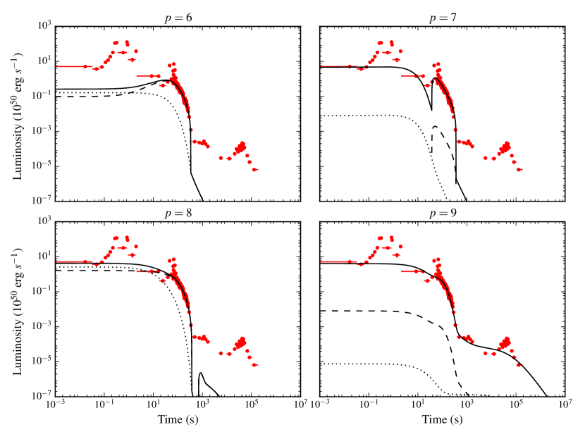
Figure 7: Models fitted to GRB 050724 with n=100𝑛100n=100 and p=6𝑝6p=6 (top left), 777 (top right), 888 (bottom left), and 999 (bottom right). Solid line - total luminosity; dashed line - propeller luminosity; dotted line - dipole luminosity; red points - combined BAT and XRT data.

Fig. 7 shows a comparison of fits with varying p𝑝p to GRB 050724 for n=100𝑛100n=100. For p=6𝑝6p=6, the model does a reasonable job of fitting the high luminosity at early times but does not retain enough energy to fit the tail. The fit demanded a large amount of fallback, δ=1.650.62+1.26𝛿subscriptsuperscript1.651.260.62\delta=1.65^{+1.26}_{-0.62}, on a short timescale, ϵ=0.130.02+0.04italic-ϵsubscriptsuperscript0.130.040.02\epsilon=0.13^{+0.04}_{-0.02}, and a very rapid spin period, P=0.69𝑃0.69P=0.69 ms (limit), in order to reach such a high luminosity so soon. Since the fallback mass reaches the disc quickly, there is nothing left in the fallback budget to provide energy for the late-time emission. p=7𝑝7p=7 and 888 provide improved fits to the early-time luminosity but again fail to fit the fading tail despite the additional parameters being pushed to the higher end of their limits, e.g. 1/fB=57871+211subscript𝑓Bsubscriptsuperscript57821711/f_{\rm B}=578^{+21}_{-71} for p=7𝑝7p=7 and ηprop=995+1subscript𝜂propsubscriptsuperscript9915\eta_{\rm prop}=99^{+1}_{-5}% for p=8𝑝8p=8 (ηdip=122+2%)subscript𝜂dippercentsubscriptsuperscript1222\left(\eta_{\rm dip}=12^{+2}_{-2}\%\right). p=9𝑝9p=9 is the only model that succeeds in fitting the tail but still requires a highly efficient emission mechanism for the propeller, ηprop=8618+13subscript𝜂propsubscriptsuperscript861318\eta_{\rm prop}=86^{+13}_{-18}%, and a very narrow beaming angle, 1/fB=502103+931subscript𝑓Bsubscriptsuperscript502931031/f_{\rm B}=502^{+93}_{-103}.

It is interesting to note the late-time giant flare within the tail of GRB 050724 that the model has not been able to fit. At present, the phenomena that cause such large outbursts at these late times are still poorly understood (see Falcone et al. 2006, Curran et al. 2008, and Chincarini et al. 2010).

5.2 GRB 060614

GRB 060614 poses a challenge to typical long/short classification scheme since it has a duration of 100similar-toabsent100\sim 100 s but the hard spectrum and lack of supernova connection are more indicative of the short classification (Mangano et al., 2007; Zhang et al., 2007; Xu et al., 2009).
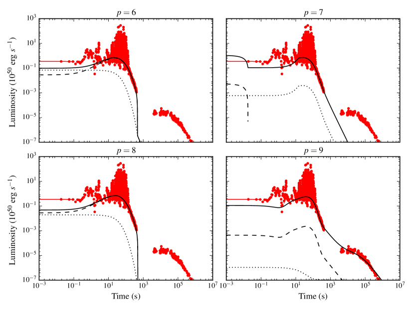
Refer to caption
Figure 8: Models fitted to GRB 060614 with n=100𝑛100n=100 and p=6𝑝6p=6 (top left), 777 (top right), 888 (bottom left), and 999 (bottom right). Solid line - total luminosity; dashed line - propeller luminosity; dotted line - dipole luminosity; red points - combined BAT and XRT data.

Fig. 8 presents model fits of varying p𝑝p and n=100𝑛100n=100 to data for GRB 060614. p=6𝑝6p=6 provides a good fit to the early-time luminosity but after 100similar-toabsent100\sim 100 s, its energy reservoir is depleted and the light curve rapidly drops off before fitting the tail. This demands a rapid spin period, P=0.900.01+0.01𝑃subscriptsuperscript0.900.010.01P=0.90^{+0.01}_{-0.01} ms, and a large amount of fallback mass, δ=49.611.63+0.38𝛿subscriptsuperscript49.610.381.63\delta=49.61^{+0.38}_{-1.63}, reaching the disc on a short timescale, ϵ=0.310.03+0.03italic-ϵsubscriptsuperscript0.310.030.03\epsilon=0.31^{+0.03}_{-0.03}. p=7𝑝7p=7 adds more structure to the early-time luminosity and has a more gradual decrease of emission but still fails to reach the tail, whereas, p=8𝑝8p=8 is very much a repeat of p=6𝑝6p=6 and offers no improvement. Again, p=9𝑝9p=9 offers the best results for fitting to the tail but requires a very efficient emission mechanism for the propeller, ηprop=100%subscript𝜂proppercent100\eta_{\rm prop}=100\% (limit), and a moderate beaming fraction, 1/fB=2517+61subscript𝑓Bsubscriptsuperscript251671/f_{\rm B}=251^{+6}_{-7}. Oddly, this model requires the least efficient dipole emission as well, ηdip=1%subscript𝜂dippercent1\eta_{\rm dip}=1\% (limit). This is probably due to the difference in EE and dipole luminosity being the greatest in GRB 060614 and so the model has to do something to achieve a drop in luminosity spanning several orders of magnitude while maintaining parameters that can produce bright, early emission.

GRB 060614 continues to be a very odd case when we examine its best fit parameters in Table 7 relating to the fit in Fig. 6 and n=10𝑛10n=10. It is one of the slowest rotating candidates with one of the most massive and most slowly fed discs. Also, the dipole and propeller emission efficiencies have completely reversed roles with ηdip=994+1%subscript𝜂dippercentsubscriptsuperscript9914\eta_{\rm dip}=99^{+1}_{-4}\% and ηprop=1%subscript𝜂proppercent1\eta_{\rm prop}=1\% (limit). The propeller’s main job is to modulate the spin in order to achieve the desired luminosities. Since the propeller plays no role in this particular fit, this indicates that that has been completely taken over by the fallback.

5.3 GRB 111121A
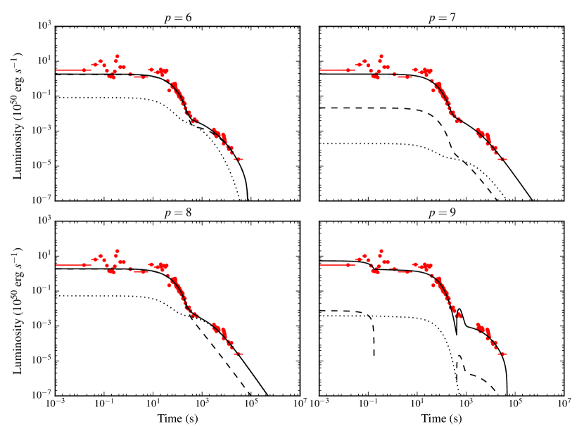
Refer to caption
Figure 9: Models fitted to GRB 111121A with n=100𝑛100n=100 and p=6𝑝6p=6 (top left), 777 (top right), 888 (bottom left), and 999 (bottom right). Solid line - total luminosity; dashed line - propeller luminosity; dotted line - dipole luminosity; red points - combined BAT and XRT data.

Fig. 9 presents model fits of varying p𝑝p and n=100𝑛100n=100 to data for GRB 111121A. This is an example of the model behaving well across all values of p𝑝p. Despite the fits for p=6,7𝑝67p=6,~{}7 and 888 looking very similar, the parameters derived from the fits vary quite significantly. For p=6𝑝6p=6 and 888, relatively small values of magnetic field are recovered, B=(2.000.11+0.12)×1015𝐵subscriptsuperscript2.000.120.11superscript1015B=\left(2.00^{+0.12}_{-0.11}\right)\times 10^{15} G and B=(1.530.31+1.40)×1015𝐵subscriptsuperscript1.531.400.31superscript1015B=\left(1.53^{+1.40}_{-0.31}\right)\times 10^{15} G respectively, whereas p=7𝑝7p=7 has a large magnetic field of B=(8.154.65+1.77)×1015𝐵subscriptsuperscript8.151.774.65superscript1015B=\left(8.15^{+1.77}_{-4.65}\right)\times 10^{15} G. The initial spin values for these fits also follow a similar pattern with spins near the break-up limit for p=6𝑝6p=6 and 888, Pi=0.69subscript𝑃i0.69P_{\rm i}=0.69 ms (limit) and Pi=0.890.17+0.16subscript𝑃isubscriptsuperscript0.890.160.17P_{\rm i}=0.89^{+0.16}_{-0.17} ms respectively, and a much slower spin for p=7𝑝7p=7, Pi=6.363.76+1.96subscript𝑃isubscriptsuperscript6.361.963.76P_{\rm i}=6.36^{+1.96}_{-3.76} ms.

Lastly, the p=9𝑝9p=9 fit has derived parameters in the moderate region of parameter space, B=(4.190.28+0.32)×1015𝐵subscriptsuperscript4.190.320.28superscript1015B=\left(4.19^{+0.32}_{-0.28}\right)\times 10^{15} G and Pi=4.380.46+0.64subscript𝑃isubscriptsuperscript4.380.640.46P_{\rm i}=4.38^{+0.64}_{-0.46} ms. It has a slowly fed disc with a small amount of fallback mass, ϵ=99.5923.43+30.58italic-ϵsubscriptsuperscript99.5930.5823.43\epsilon=99.59^{+30.58}_{-23.43} and δ=(2.840.33+0.36)×103𝛿subscriptsuperscript2.840.360.33superscript103\delta=\left(2.84^{+0.36}_{-0.33}\right)\times 10^{-3}. We derive a propeller efficiency consistent with the value used to Gompertz et al. (2014) of ηprop=41.4813.27+11.99%subscript𝜂proppercentsubscriptsuperscript41.4811.9913.27\eta_{\rm prop}=41.48^{+11.99}_{-13.27}\% but the fit requires a much higher dipole efficiency of ηdip=83.6031.94+15.65%subscript𝜂dippercentsubscriptsuperscript83.6015.6531.94\eta_{\rm dip}=83.60^{+15.65}_{-31.94}\% and a narrow jet opening angle of 1/fB=474180+1201subscript𝑓Bsubscriptsuperscript4741201801/f_{\rm B}=474^{+120}_{-180}. However, this fit has introduced a flare at roughly the 100010001000 s mark which could be indicative of over-fitting.

5.4 Refitting excluding early-time data

The results presented in Table 7 are consistently pushing the upper bounds for the initial disc mass, MD,isubscript𝑀DiM_{\rm D,i}. This is most likely due to the model’s need to have a high accretion rate at early-times in order to reach the high luminosities at those times. Since the emission produced at these times is usually attributed to internal shocks and energy drawn from the merger rather than magnetic particle acceleration, fitting these high early-time luminosities may not strictly be within the remit of the model. We therefore chose to refit the sample excluding some of the early-time data.

We chose an arbitrary cut-off of 101010 seconds to define the on-set of EE after the prompt emission. This meant we avoided making an arbitrary cut for each individual burst since EE isn’t currently well defined. The fits were performed for p=6,7,8𝑝678p=6,~{}7,~{}8 and 999 and n=1𝑛1n=1 for comparison with the work in Gompertz et al. (2014).

Table 8: AICc values for fits to the SGRBEE sample with varying p𝑝p values and n=1𝑛1n=1 with data <10absent10<10s excluded. Values in bold face are the minimum value for each GRB. GRB 061210 has fewer data points than free parameters resulting in a negative AICc value which was not considered when choosing the best fit.
GRB p=6𝑝6p=6 p=7𝑝7p=7 p=8𝑝8p=8 p=9𝑝9p=9
050724 1,61116111,611 1,48914891,489 1,56115611,561 𝟏,𝟐𝟓𝟗12591,259
051016B 340340340 252252252 310310310 𝟏𝟓𝟑153153
051227 178178178 𝟓𝟑5353 595959 707070
060614 48,0864808648,086 43,7384373843,738 43,7284372843,728 𝟒𝟑,𝟔𝟏𝟎4361043,610
061006 177177177 𝟗𝟎9090 114114114 123123123
061210 17superscript17-17^{*} 181181181 𝟔𝟔6666 357357357
070714B 203203203 215215215 𝟏𝟕𝟕177177 195195195
071227 112112112 𝟖𝟗8989 100100100 101101101
080123 354354354 308308308 𝟐𝟗𝟖298298 319319319
080503 2,28122812,281 2,37523752,375 𝟐,𝟏𝟓𝟕21572,157 2,33923392,339
100212A 8,19881988,198 7,60276027,602 7,77177717,771 𝟕,𝟎𝟕𝟑70737,073
100522A 8,53085308,530 7,40174017,401 7,72577257,725 𝟔,𝟑𝟐𝟐63226,322
111121A 872872872 𝟕𝟖𝟐782782 819819819 787787787
150424A 366366366 279279279 354354354 𝟐𝟓𝟏251251
160410A 495495495 𝟏𝟒𝟗149149 212212212 222222222
Refer to caption
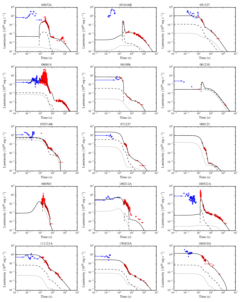
Figure 10: Global best fit models produced from fitting to the SGRBEE sample for n=1𝑛1n=1 and excluding data <10absent10<10 s (bold values in Table 8). Solid, black line - total luminosity; dashed, black line - propeller luminosity; dotted, black line - dipole luminosity. Points are combined BAT and XRT data: red points have been included in the fitting, blue points were excluded.

Table 8 presents the AICc values of the refits. The best fits (bold values) from Table 8 are plotted in Fig. 10 and the parameters derived from these fits are presented in Table 9 with the χred2subscriptsuperscript𝜒2red\chi^{2}_{\rm red} goodness of fit statistic. GRB 061210 has very few data points and excluding data <10absent10<10 seconds means that there are fewer data points than free parameters which resulted in negative AICc and χred2subscriptsuperscript𝜒2red\chi^{2}_{\rm red} values. Therefore, it is shown here for consistency rather than as a statistically significant result.

Table 9: Parameters derived from the best fitting models to the SGRBEE sample for n=1𝑛1n=1 and excluding data <10absent10<10s. Uncertainties represent a 95% confidence interval. Values marked with an [L] are a parameter limit; those marked with an [F] were fixed during fitting. χred2subscriptsuperscript𝜒2red\chi^{2}_{\rm red} values are shown to indicate goodness of fit. GRB 061210 has fewer data points than free parameters resulting in a negative χred2subscriptsuperscript𝜒2red\chi^{2}_{\rm red} value.
GRB B𝐵B Pisubscript𝑃iP_{\rm i} MD,isubscript𝑀DiM_{\rm D,i} RDsubscript𝑅DR_{\rm D} ϵitalic-ϵ\epsilon δ𝛿\delta ηdipsubscript𝜂dip\eta_{\rm dip} ηpropsubscript𝜂prop\eta_{\rm prop} 1/fB1subscript𝑓B1/f_{\rm B} χred2subscriptsuperscript𝜒2red\chi^{2}_{\rm red}
(×1015absentsuperscript1015\times 10^{-15} G) (ms) (×102M)\left(\times 10^{-2}~{}M_{\odot}\right) (km) (%) (%)
050724 3.300.36+0.48subscriptsuperscript3.300.480.363.30^{+0.48}_{-0.36} 9.940.26+0.06subscriptsuperscript9.940.060.269.94^{+0.06}_{-0.26} 0.1670.028+0.042subscriptsuperscript0.1670.0420.0280.167^{+0.042}_{-0.028} 3837+7subscriptsuperscript38377383^{+7}_{-7} 0.940.83+12.75subscriptsuperscript0.9412.750.830.94^{+12.75}_{-0.83} (0.850.73+3.15)×103subscriptsuperscript0.853.150.73superscript103\left(0.85^{+3.15}_{-0.73}\right)\times 10^{-3} 111[L] 988+2subscriptsuperscript982898^{+2}_{-8} 25322+35subscriptsuperscript2533522253^{+35}_{-22} 555
051016B 1.180.48+0.68subscriptsuperscript1.180.680.481.18^{+0.68}_{-0.48} 9.092.84+0.87subscriptsuperscript9.090.872.849.09^{+0.87}_{-2.84} 2.471.63+4.73subscriptsuperscript2.474.731.632.47^{+4.73}_{-1.63} 593+4subscriptsuperscript594359^{+4}_{-3} 635.72216.98+234.17subscriptsuperscript635.72234.17216.98635.72^{+234.17}_{-216.98} (1.000.51+0.91)×103subscriptsuperscript1.000.910.51superscript103\left(1.00^{+0.91}_{-0.51}\right)\times 10^{-3} 111[L] 9420+6subscriptsuperscript9462094^{+6}_{-20} 220144+296subscriptsuperscript220296144220^{+296}_{-144} 222
051227 8.863.19+1.10subscriptsuperscript8.861.103.198.86^{+1.10}_{-3.19} 4.001.84+1.66subscriptsuperscript4.001.661.844.00^{+1.66}_{-1.84} 0.670.31+1.84subscriptsuperscript0.671.840.310.67^{+1.84}_{-0.31} 13426+35subscriptsuperscript1343526134^{+35}_{-26} 4.984.86+456.99subscriptsuperscript4.98456.994.864.98^{+456.99}_{-4.86} (0.300.30+1.31)×101subscriptsuperscript0.301.310.30superscript101\left(0.30^{+1.31}_{-0.30}\right)\times 10^{-1} 555[F] 404040[F] 8257+77subscriptsuperscript82775782^{+77}_{-57} 222
060614 6.211.03+0.41subscriptsuperscript6.210.411.036.21^{+0.41}_{-1.03} 8.302.48+1.14subscriptsuperscript8.301.142.488.30^{+1.14}_{-2.48} 0.7550.117+0.453subscriptsuperscript0.7550.4530.1170.755^{+0.453}_{-0.117} 168023+23subscriptsuperscript168023231680^{+23}_{-23} 562.87103.91+161.29subscriptsuperscript562.87161.29103.91562.87^{+161.29}_{-103.91} (1.000.10+0.14)×102subscriptsuperscript1.000.140.10superscript102\left(1.00^{+0.14}_{-0.10}\right)\times 10^{-2} 8452+15subscriptsuperscript84155284^{+15}_{-52} 84+2subscriptsuperscript8248^{+2}_{-4} 506225+91subscriptsuperscript50691225506^{+91}_{-225} 202020
061006 7.161.07+0.81subscriptsuperscript7.160.811.077.16^{+0.81}_{-1.07} 7.973.97+1.63subscriptsuperscript7.971.633.977.97^{+1.63}_{-3.97} 2.070.56+3.29subscriptsuperscript2.073.290.562.07^{+3.29}_{-0.56} 1908372+89subscriptsuperscript1908893721908^{+89}_{-372} 136.0554.63+94.65subscriptsuperscript136.0594.6554.63136.05^{+94.65}_{-54.63} 20.985.34+7.99subscriptsuperscript20.987.995.3420.98^{+7.99}_{-5.34} 555[F] 404040[F] 380311+209subscriptsuperscript380209311380^{+209}_{-311} 888
061210 0.750.24+0.27subscriptsuperscript0.750.270.240.75^{+0.27}_{-0.24} 0.800.11+0.26subscriptsuperscript0.800.260.110.80^{+0.26}_{-0.11} 7.042.20+2.76subscriptsuperscript7.042.762.207.04^{+2.76}_{-2.20} 12842+143subscriptsuperscript12814342128^{+143}_{-42} 182.82165.31+748.09subscriptsuperscript182.82748.09165.31182.82^{+748.09}_{-165.31} (1.471.13+6.69)×101subscriptsuperscript1.476.691.13superscript101\left(1.47^{+6.69}_{-1.13}\right)\times 10^{-1} 73+3subscriptsuperscript7337^{+3}_{-3} 9125+9subscriptsuperscript9192591^{+9}_{-25} 111[F] 33superscript33-33^{*}
070714B 4.971.45+1.20subscriptsuperscript4.971.201.454.97^{+1.20}_{-1.45} 1.000.27+0.15subscriptsuperscript1.000.150.271.00^{+0.15}_{-0.27} 4.240.90+2.93subscriptsuperscript4.242.930.904.24^{+2.93}_{-0.90} 32025+29subscriptsuperscript3202925320^{+29}_{-25} 520.96494.48+453.38subscriptsuperscript520.96453.38494.48520.96^{+453.38}_{-494.48} (1.550.65+0.92)×101subscriptsuperscript1.550.920.65superscript101\left(1.55^{+0.92}_{-0.65}\right)\times 10^{-1} 4831+42subscriptsuperscript48423148^{+42}_{-31} 8036+19subscriptsuperscript80193680^{+19}_{-36} 111[F] 222
071227 8.402.37+1.52subscriptsuperscript8.401.522.378.40^{+1.52}_{-2.37} 1.790.80+1.99subscriptsuperscript1.791.990.801.79^{+1.99}_{-0.80} 4.982.80+4.42subscriptsuperscript4.984.422.804.98^{+4.42}_{-2.80} 25023+25subscriptsuperscript2502523250^{+25}_{-23} 1.781.67+28.53subscriptsuperscript1.7828.531.671.78^{+28.53}_{-1.67} (0.950.61+4.28)×103subscriptsuperscript0.954.280.61superscript103\left(0.95^{+4.28}_{-0.61}\right)\times 10^{-3} 555[F] 404040[F] 4933+51subscriptsuperscript49513349^{+51}_{-33} 222
080123 7.080.25+0.18subscriptsuperscript7.080.180.257.08^{+0.18}_{-0.25} 0.910.04+0.07subscriptsuperscript0.910.070.040.91^{+0.07}_{-0.04} 9.840.61+0.16subscriptsuperscript9.840.160.619.84^{+0.16}_{-0.61} 2544+5subscriptsuperscript25454254^{+5}_{-4} 62.0358.06+117.14subscriptsuperscript62.03117.1458.0662.03^{+117.14}_{-58.06} (1.561.19+1.90)×104subscriptsuperscript1.561.901.19superscript104\left(1.56^{+1.90}_{-1.19}\right)\times 10^{-4} 43+3subscriptsuperscript4334^{+3}_{-3} 989+2subscriptsuperscript982998^{+2}_{-9} 111[F] 666
080503 5.451.29+0.55subscriptsuperscript5.450.551.295.45^{+0.55}_{-1.29} 6.954.62+2.91subscriptsuperscript6.952.914.626.95^{+2.91}_{-4.62} 6.275.58+3.61subscriptsuperscript6.273.615.586.27^{+3.61}_{-5.58} 595+2subscriptsuperscript592559^{+2}_{-5} 0.1080.008+0.079subscriptsuperscript0.1080.0790.0080.108^{+0.079}_{-0.008} 4.212.15+37.64subscriptsuperscript4.2137.642.154.21^{+37.64}_{-2.15} 7354+26subscriptsuperscript73265473^{+26}_{-54} 6036+20subscriptsuperscript60203660^{+20}_{-36} 111[F] 999
100212A 9.980.07+0.02subscriptsuperscript9.980.020.079.98^{+0.02}_{-0.07} 7.504.32+2.39subscriptsuperscript7.502.394.327.50^{+2.39}_{-4.32} 9.960.17+0.04subscriptsuperscript9.960.040.179.96^{+0.04}_{-0.17} 1631+1subscriptsuperscript16311163^{+1}_{-1} 980.0587.98+19.22subscriptsuperscript980.0519.2287.98980.05^{+19.22}_{-87.98} (7.070.62+0.23)×101subscriptsuperscript7.070.230.62superscript101\left(7.07^{+0.23}_{-0.62}\right)\times 10^{-1} 7920+20subscriptsuperscript79202079^{+20}_{-20} 174+5subscriptsuperscript175417^{+5}_{-4} 44194+148subscriptsuperscript44114894441^{+148}_{-94} 191919
100522A 3.060.07+0.09subscriptsuperscript3.060.090.073.06^{+0.09}_{-0.07} 9.930.33+0.07subscriptsuperscript9.930.070.339.93^{+0.07}_{-0.33} 0.5090.105+0.076subscriptsuperscript0.5090.0760.1050.509^{+0.076}_{-0.105} 631+2subscriptsuperscript632163^{+2}_{-1} 0.220.11+1.21subscriptsuperscript0.221.210.110.22^{+1.21}_{-0.11} (3.111.87+2.10)×103subscriptsuperscript3.112.101.87superscript103\left(3.11^{+2.10}_{-1.87}\right)\times 10^{-3} 111[L] 993+1subscriptsuperscript991399^{+1}_{-3} 31619+26subscriptsuperscript3162619316^{+26}_{-19} 373737
111121A 9.032.25+0.92subscriptsuperscript9.030.922.259.03^{+0.92}_{-2.25} 6.342.71+1.64subscriptsuperscript6.341.642.716.34^{+1.64}_{-2.71} 1.140.31+1.22subscriptsuperscript1.141.220.311.14^{+1.22}_{-0.31} 29214+16subscriptsuperscript2921614292^{+16}_{-14} 32.445.21+7.02subscriptsuperscript32.447.025.2132.44^{+7.02}_{-5.21} (1.770.26+0.36)×102subscriptsuperscript1.770.360.26superscript102\left(1.77^{+0.36}_{-0.26}\right)\times 10^{-2} 555[F] 404040[F] 247167+119subscriptsuperscript247119167247^{+119}_{-167} 777
150424A 9.191.03+0.68subscriptsuperscript9.190.681.039.19^{+0.68}_{-1.03} 8.992.76+0.97subscriptsuperscript8.990.972.768.99^{+0.97}_{-2.76} 0.5440.115+0.421subscriptsuperscript0.5440.4210.1150.544^{+0.421}_{-0.115} 43443+61subscriptsuperscript4346143434^{+61}_{-43} 20.407.56+9.75subscriptsuperscript20.409.757.5620.40^{+9.75}_{-7.56} (1.880.59+0.66)×102subscriptsuperscript1.880.660.59superscript102\left(1.88^{+0.66}_{-0.59}\right)\times 10^{-2} 6145+37subscriptsuperscript61374561^{+37}_{-45} 139+14subscriptsuperscript1314913^{+14}_{-9} 12269+331subscriptsuperscript12233169122^{+331}_{-69} 222
160410A 3.580.95+0.63subscriptsuperscript3.580.630.953.58^{+0.63}_{-0.95} 3.171.43+0.80subscriptsuperscript3.170.801.433.17^{+0.80}_{-1.43} 3.320.89+3.94subscriptsuperscript3.323.940.893.32^{+3.94}_{-0.89} 82687+79subscriptsuperscript8267987826^{+79}_{-87} 21.8319.02+199.41subscriptsuperscript21.83199.4119.0221.83^{+199.41}_{-19.02} (3.652.19+5.63)×102subscriptsuperscript3.655.632.19superscript102\left(3.65^{+5.63}_{-2.19}\right)\times 10^{-2} 555[F] 404040[F] 410285+181subscriptsuperscript410181285410^{+181}_{-285} 333

As is shown in Fig. 10, the result of excluding the early-time data is to produce more light curves of the humped morphology than the sloped or classic variety in Fig. 6. But most surprisingly, this experiment did not succeed in reducing MD,isubscript𝑀DiM_{\rm D,i} as expected, suggesting the extra mass is a result of another change in the model, most likely the use of Equation (13) instead of Equation (14). Equation (14) enhances the dipole spin-down and mass-loss resulting in a lower initial disc mass.

5.5 Refitting with enhanced dipole torque

For direct comparison with Gompertz et al. (2014), the sample was fitted once more using the enhanced dipole torque in Equation (14) from Bucciantini et al. (2006) for n=1𝑛1n=1 and p=6,7,8𝑝678p=6,~{}7,~{}8 and 999. The AICc values for the fits are presented in Table 10, the best fits from this table are shown in Fig. 11, and the parameters derived from those fits are presented in Table 11.

Table 10: AICc values for fits to the SGRBEE sample excluding data <10absent10<10 s and using Equation (14) for the dipole torque. GRB 061210 has fewer data points than free parameters and so these statistics should be treat with caution.
GRB p=6𝑝6p=6 p=7𝑝7p=7 p=8𝑝8p=8 p=9𝑝9p=9
050724 5,92759275,927 17,5161751617,516 1,63616361,636 𝟏,𝟐𝟖𝟕12871,287
051016B 396396396 2,32723272,327 444444444 𝟏𝟒𝟕147147
051227 493493493 1,00010001,000 192192192 𝟔𝟒6464
060614 50,6875068750,687 88,4498844988,449 44,0554405544,055 𝟒𝟑,𝟔𝟔𝟕4366743,667
061006 294294294 854854854 424424424 𝟏𝟏𝟏111111
061210 372372372 1,23612361,236 𝟗𝟔9696 1,53215321,532
070714B 880880880 3,62236223,622 𝟐𝟏𝟐212212 1,40214021,402
071227 𝟏𝟏𝟓115115 1,29312931,293 161161161 202202202
080123 355355355 6,16261626,162 752752752 𝟐𝟗𝟎290290
080503 3,18631863,186 13,2991329913,299 𝟐,𝟑𝟑𝟔23362,336 3,67036703,670
100212A 9,03590359,035 35,0743507435,074 8,75787578,757 𝟖,𝟎𝟑𝟕80378,037
100522A 8,70987098,709 22,4892248922,489 8,80888088,808 𝟔,𝟑𝟗𝟏63916,391
111121A 2,49824982,498 8,44184418,441 898898898 𝟕𝟓𝟕757757
150424A 398398398 5,86158615,861 𝟐𝟓𝟐252252 267267267
160410A 1,19811981,198 1,47914791,479 𝟕𝟏𝟕717717 971971971
Refer to caption
Figure 11: Results of fitting to the SGRBEE sample for the best global fits (bold values in Table 10) excluding data <10absent10<10s and using Equation (14) for the dipole torque. Solid, black line - total luminosity; dashed, black line - propeller luminosity; dotted, black line - dipole luminosity. Data points are combined BAT and XRT data: blue points have been excluded from the fit, red points were included.
Table 11: Parameters derived from fits to SGRBEE sample for the globals fits (bold values in Table 10) excluding data <10absent10<10s and using Equation (14) for the dipole torque. Uncertainties are a 95%percent9595\% confidence interval and values marked with an [L] are a parameter limit. GRB 061210 has fewer data points than parameters resulting in a negative χred2subscriptsuperscript𝜒2red\chi^{2}_{\rm red} value.
GRB B𝐵B Pisubscript𝑃iP_{\rm i} MD,isubscript𝑀DiM_{\rm D,i} RDsubscript𝑅DR_{\rm D} ϵitalic-ϵ\epsilon δ𝛿\delta ηdipsubscript𝜂dip\eta_{\rm dip} ηpropsubscript𝜂prop\eta_{\rm prop} 1/fB1subscript𝑓B1/f_{\rm B} χred2subscriptsuperscript𝜒2red\chi^{2}_{\rm red}
(×1015absentsuperscript1015\times 10^{15} G) (ms) (×102M)\left(\times 10^{-2}~{}M_{\odot}\right) (km) (%) (%)
050724 2.750.31+0.26subscriptsuperscript2.750.260.312.75^{+0.26}_{-0.31} 8.911.12+0.63subscriptsuperscript8.910.631.128.91^{+0.63}_{-1.12} 0.1000.005+0.021subscriptsuperscript0.1000.0210.0050.100^{+0.021}_{-0.005} 3788+8subscriptsuperscript37888378^{+8}_{-8} 983.7667.62+15.64subscriptsuperscript983.7615.6467.62983.76^{+15.64}_{-67.62} (5.701.13+1.15)×103subscriptsuperscript5.701.151.13superscript103\left(5.70^{+1.15}_{-1.13}\right)\times 10^{-3} 111[L] 9710+3subscriptsuperscript9731097^{+3}_{-10} 522128+73subscriptsuperscript52273128522^{+73}_{-128} 555
051016B 0.360.09+0.20subscriptsuperscript0.360.200.090.36^{+0.20}_{-0.09} 2.330.57+0.61subscriptsuperscript2.330.610.572.33^{+0.61}_{-0.57} 2.621.56+2.35subscriptsuperscript2.622.351.562.62^{+2.35}_{-1.56} 522+5subscriptsuperscript525252^{+5}_{-2} 772.31259.35+205.95subscriptsuperscript772.31205.95259.35772.31^{+205.95}_{-259.35} (4.151.97+5.45)×104subscriptsuperscript4.155.451.97superscript104\left(4.15^{+5.45}_{-1.97}\right)\times 10^{-4} 111[L] 9223+7subscriptsuperscript9272392^{+7}_{-23} 524213+73subscriptsuperscript52473213524^{+73}_{-213} 222
051227 8.123.86+1.80subscriptsuperscript8.121.803.868.12^{+1.80}_{-3.86} 4.913.01+3.23subscriptsuperscript4.913.233.014.91^{+3.23}_{-3.01} 0.260.15+0.87subscriptsuperscript0.260.870.150.26^{+0.87}_{-0.15} 15940+60subscriptsuperscript1596040159^{+60}_{-40} 13.3213.21+732.02subscriptsuperscript13.32732.0213.2113.32^{+732.02}_{-13.21} (0.770.77+6.62)×102subscriptsuperscript0.776.620.77superscript102\left(0.77^{+6.62}_{-0.77}\right)\times 10^{-2} 4536+51subscriptsuperscript45513645^{+51}_{-36} 5344+44subscriptsuperscript53444453^{+44}_{-44} 238187+327subscriptsuperscript238327187238^{+327}_{-187} 222
060614 3.030.39+0.36subscriptsuperscript3.030.360.393.03^{+0.36}_{-0.39} 6.051.42+1.60subscriptsuperscript6.051.601.426.05^{+1.60}_{-1.42} 0.310.08+0.13subscriptsuperscript0.310.130.080.31^{+0.13}_{-0.08} 129717+17subscriptsuperscript129717171297^{+17}_{-17} 632.65105.42+119.29subscriptsuperscript632.65119.29105.42632.65^{+119.29}_{-105.42} (1.530.14+0.14)×102subscriptsuperscript1.530.140.14superscript102\left(1.53^{+0.14}_{-0.14}\right)\times 10^{-2} 8041+19subscriptsuperscript80194180^{+19}_{-41} 198+10subscriptsuperscript1910819^{+10}_{-8} 383222+208subscriptsuperscript383208222383^{+208}_{-222} 202020
061006 3.570.75+0.61subscriptsuperscript3.570.610.753.57^{+0.61}_{-0.75} 2.671.02+0.93subscriptsuperscript2.670.931.022.67^{+0.93}_{-1.02} 1.080.36+0.96subscriptsuperscript1.080.960.361.08^{+0.96}_{-0.36} 42314+15subscriptsuperscript4231514423^{+15}_{-14} 52.7129.47+51.20subscriptsuperscript52.7151.2029.4752.71^{+51.20}_{-29.47} (2.380.61+0.65)×103subscriptsuperscript2.380.650.61superscript103\left(2.38^{+0.65}_{-0.61}\right)\times 10^{-3} 7348+26subscriptsuperscript73264873^{+26}_{-48} 63+6subscriptsuperscript6636^{+6}_{-3} 347273+240subscriptsuperscript347240273347^{+240}_{-273} 111111
061210 0.400.03+0.03subscriptsuperscript0.400.030.030.40^{+0.03}_{-0.03} 0.690.690.69[L] 1.190.22+0.25subscriptsuperscript1.190.250.221.19^{+0.25}_{-0.22} 21159+89subscriptsuperscript2118959211^{+89}_{-59} 815.21528.85+177.54subscriptsuperscript815.21177.54528.85815.21^{+177.54}_{-528.85} (3.210.88+3.07)×101subscriptsuperscript3.213.070.88superscript101\left(3.21^{+3.07}_{-0.88}\right)\times 10^{-1} 173+3subscriptsuperscript173317^{+3}_{-3} 993+1subscriptsuperscript991399^{+1}_{-3} 111[F] 43superscript43-43^{*}
070714B 1.770.15+0.17subscriptsuperscript1.770.170.151.77^{+0.17}_{-0.15} 0.690.690.69[L] 3.430.82+0.38subscriptsuperscript3.430.380.823.43^{+0.38}_{-0.82} 30722+26subscriptsuperscript3072622307^{+26}_{-22} 41.8321.04+598.49subscriptsuperscript41.83598.4921.0441.83^{+598.49}_{-21.04} (1.210.32+0.92)×101subscriptsuperscript1.210.920.32superscript101\left(1.21^{+0.92}_{-0.32}\right)\times 10^{-1} 7559+24subscriptsuperscript75245975^{+24}_{-59} 995+1subscriptsuperscript991599^{+1}_{-5} 111[F] 222
071227 1.190.13+0.27subscriptsuperscript1.190.270.131.19^{+0.27}_{-0.13} 0.700.01+0.04subscriptsuperscript0.700.040.010.70^{+0.04}_{-0.01} 5.460.60+0.20subscriptsuperscript5.460.200.605.46^{+0.20}_{-0.60} 1144116+97subscriptsuperscript1144971161144^{+97}_{-116} 250.23225.49+674.92subscriptsuperscript250.23674.92225.49250.23^{+674.92}_{-225.49} (0.200.13+1.25)×101subscriptsuperscript0.201.250.13superscript101\left(0.20^{+1.25}_{-0.13}\right)\times 10^{-1} 555[F] 404040[F] 111[F] 333
080123 8.312.20+1.61subscriptsuperscript8.311.612.208.31^{+1.61}_{-2.20} 5.672.52+2.71subscriptsuperscript5.672.712.525.67^{+2.71}_{-2.52} 0.320.13+0.38subscriptsuperscript0.320.380.130.32^{+0.38}_{-0.13} 2446+7subscriptsuperscript24476244^{+7}_{-6} 54.1448.87+91.66subscriptsuperscript54.1491.6648.8754.14^{+91.66}_{-48.87} (1.260.60+1.09)×104subscriptsuperscript1.261.090.60superscript104\left(1.26^{+1.09}_{-0.60}\right)\times 10^{-4} 43+7subscriptsuperscript4734^{+7}_{-3} 6640+32subscriptsuperscript66324066^{+32}_{-40} 154112+351subscriptsuperscript154351112154^{+351}_{-112} 666
080503 9.104.06+0.87subscriptsuperscript9.100.874.069.10^{+0.87}_{-4.06} 1.060.35+0.74subscriptsuperscript1.060.740.351.06^{+0.74}_{-0.35} 0.750.12+0.92subscriptsuperscript0.750.920.120.75^{+0.92}_{-0.12} 76740+23subscriptsuperscript7672340767^{+23}_{-40} 36.8936.76+828.92subscriptsuperscript36.89828.9236.7636.89^{+828.92}_{-36.76} (0.010.01+16.16)×101subscriptsuperscript0.0116.160.01superscript101\left(0.01^{+16.16}_{-0.01}\right)\times 10^{-1} 21+3subscriptsuperscript2312^{+3}_{-1} 6843+21subscriptsuperscript68214368^{+21}_{-43} 111[F] 999
100212A 0.730.07+0.08subscriptsuperscript0.730.080.070.73^{+0.08}_{-0.07} 3.910.34+0.37subscriptsuperscript3.910.370.343.91^{+0.37}_{-0.34} 0.110.01+0.02subscriptsuperscript0.110.020.010.11^{+0.02}_{-0.01} 55015+15subscriptsuperscript5501515550^{+15}_{-15} 0.370.25+0.95subscriptsuperscript0.370.950.250.37^{+0.95}_{-0.25} (2.461.34+3.05)×102subscriptsuperscript2.463.051.34superscript102\left(2.46^{+3.05}_{-1.34}\right)\times 10^{-2} 111[L] 7726+21subscriptsuperscript77212677^{+21}_{-26} 9426+50subscriptsuperscript94502694^{+50}_{-26} 222222
100522A 1.530.12+0.29subscriptsuperscript1.530.290.121.53^{+0.29}_{-0.12} 0.740.05+0.15subscriptsuperscript0.740.150.050.74^{+0.15}_{-0.05} 8.452.38+1.22subscriptsuperscript8.451.222.388.45^{+1.22}_{-2.38} 2435+6subscriptsuperscript24365243^{+6}_{-5} 18.736.57+10.36subscriptsuperscript18.7310.366.5718.73^{+10.36}_{-6.57} (4.720.50+0.56)×103subscriptsuperscript4.720.560.50superscript103\left(4.72^{+0.56}_{-0.50}\right)\times 10^{-3} 8924+11subscriptsuperscript89112489^{+11}_{-24} 111[L] 4310+22subscriptsuperscript43221043^{+22}_{-10} 373737
111121A 2.210.22+0.26subscriptsuperscript2.210.260.222.21^{+0.26}_{-0.22} 1.450.26+0.34subscriptsuperscript1.450.340.261.45^{+0.34}_{-0.26} 1.970.51+0.64subscriptsuperscript1.970.640.511.97^{+0.64}_{-0.51} 24712+15subscriptsuperscript2471512247^{+15}_{-12} 0.200.10+0.73subscriptsuperscript0.200.730.100.20^{+0.73}_{-0.10} (5.003.18+3.77)×102subscriptsuperscript5.003.773.18superscript102\left(5.00^{+3.77}_{-3.18}\right)\times 10^{-2} 3224+22subscriptsuperscript32222432^{+22}_{-24} 6044+38subscriptsuperscript60384460^{+38}_{-44} 3518+91subscriptsuperscript35911835^{+91}_{-18} 666
150424A 0.380.07+0.08subscriptsuperscript0.380.080.070.38^{+0.08}_{-0.07} 0.750.05+0.12subscriptsuperscript0.750.120.050.75^{+0.12}_{-0.05} 0.390.04+0.11subscriptsuperscript0.390.110.040.39^{+0.11}_{-0.04} 54021+22subscriptsuperscript5402221540^{+22}_{-21} 951.95168.74+46.20subscriptsuperscript951.9546.20168.74951.95^{+46.20}_{-168.74} (5.130.84+0.88)×101subscriptsuperscript5.130.880.84superscript101\left(5.13^{+0.88}_{-0.84}\right)\times 10^{-1} 21+1subscriptsuperscript2112^{+1}_{-1} 9121+9subscriptsuperscript9192191^{+9}_{-21} 111[F] 222
160410A 1.490.13+0.14subscriptsuperscript1.490.140.131.49^{+0.14}_{-0.13} 0.690.690.69[L] 0.170.06+0.53subscriptsuperscript0.170.530.060.17^{+0.53}_{-0.06} 544322+563subscriptsuperscript544563322544^{+563}_{-322} 0.570.46+6.17subscriptsuperscript0.576.170.460.57^{+6.17}_{-0.46} 20.4216.15+22.88subscriptsuperscript20.4222.8816.1520.42^{+22.88}_{-16.15} 994+1subscriptsuperscript991499^{+1}_{-4} 100100100[L] 111[F] 171717

Including Equation (14) in the model provides a marginal improvement in fitting, e.g. the tail of GRB 100212A is matched more closely in Fig. 11 than Fig. 10, though in some cases it performs much worse, e.g. GRB 160410A. The initial disc mass MD,isubscript𝑀DiM_{\rm D,i} is reduced by approximately an order of magnitude across the sample. This is a reflection of the enhanced energy output facilitated by Equation (14). Equation (14) does not produce a dramatic change in the morphology or energetics of the fits, nor does it significantly improve the fit statistics. However, the derived disc masses are more broadly in line with previous work (e.g. Rosswog 2007).

5.6 The B-P landscape
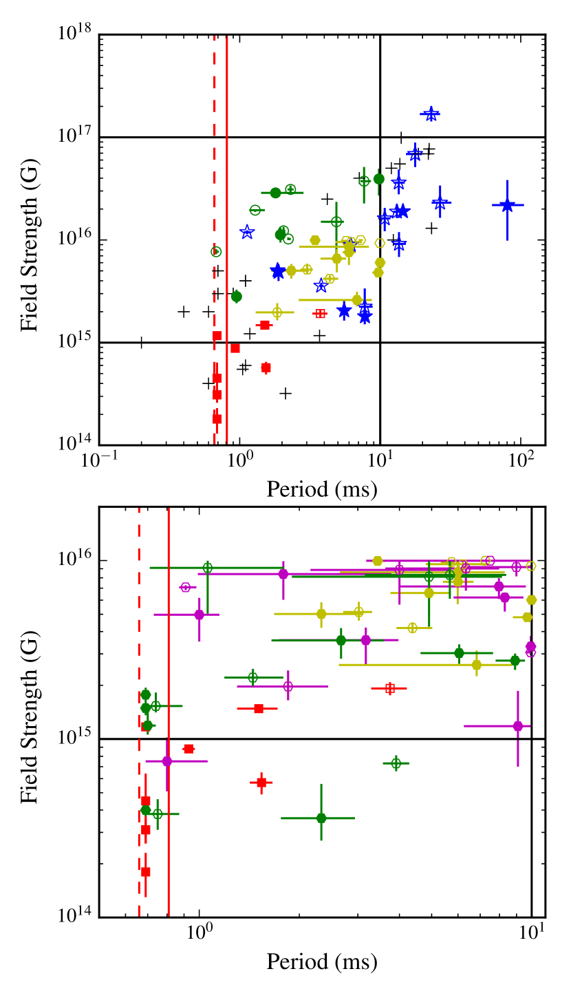
Refer to caption
Figure 12: Plots of magnetic field strength versus initial spin period. The solid (dashed) red line represents the break-up period for a collapsar (binary merger) progenitor Lattimer & Prakash (2004). Top panel - blue stars: stable magnetars and green circles: unstable magnetars which collapse to form a black hole Rowlinson et al. (2013). Black ‘+’ symbols are the LGRB candidates identified by Lyons et al. (2010); Dall’Osso et al. (2011). Red squares (both panels) show the values found in Gompertz et al. (2014). Yellow hexagons (both panels) represent the magnetic fields and initial spin periods of this work for the global best fit values in Table 7. Bottom panel - magenta hexagons are the B𝐵B and Pisubscript𝑃iP_{\rm i} values for fits excluding data <10absent10<10 s in Table 9; green hexagons are B𝐵B and Pisubscript𝑃iP_{\rm i} values for fits excluding data <10absent10<10 s and including Equation (14) in Table 11. Filled symbols have observed redshifts, open symbols use the sample average redshift, which is z=0.39𝑧0.39z=0.39 for extended bursts and z=0.72𝑧0.72z=0.72 for the short bursts from Rowlinson et al. (2013).

Fig. 12 shows where the results of this work fall in relation to other GRBs in both the long and short classifications. It needs to be noted that the results from Gompertz et al. (2014) used fixed efficiencies of ηdip=5%subscript𝜂dippercent5\eta_{\rm dip}=5\% and ηprop=40%subscript𝜂proppercent40\eta_{\rm prop}=40\%, whereas the work done in Rowlinson et al. (2013) uses 100% efficiency instead, and our efficiencies have been free parameters in most fitting procedures. Also, Gompertz et al. (2014) used Equation (14) which enhances the dipole spin-down and so these results appear to occupy their own region of low magnetic field and spin period. Hence, conclusions drawn from this plot require some caution.

However, Fig. 12 does show us that our results occupy a region of moderate to high magnetic field and spin period, indicating that the fallback accretion relaxes the constraints on the initial spin of the magnetar (i.e. it does not need to be born near the break-up period) since it will be spun-up by the fallback regardless. Though this result could be due to either the addition of a t5/3superscript𝑡53t^{-5/3} fallback accretion profile or our inclusion of beaming as a fitting parameter. The results of this work still do not approach the same same region as Gompertz et al. (2014) even when early-time, high luminosity data is excluded and Equation (14) is used which consolidates that the shift in B𝐵B-P𝑃P parameter space is due to the inclusion of fallback accretion.

6 Conclusions

We have modified the magnetar propeller model to include fallback accretion, examined the effect these changes have on model light curves and used a MCMC to fit the model to a sample of short GRBs exhibiting extended emission for a range of free parameters and “sharpness” of propeller. We have found that the parameters derived from the fits produced by the propeller model with fallback accretion are consistent with theoretical predictions for magnetars.

Our model can cope with long, dipole plateaux and flare-like variability but struggles with the early-time, short-timescale variability. However, since this variability is usually present in the prompt emission which is generally attributed to internal shocks rather than magnetic acceleration of particles, it is not strictly within the remit of the model to fit it.

The addition of fallback accretion provides a noticeable improvement in matching light curves compared to those presented in Gompertz et al. (2014) and fallback accretion may play a pivotal role in explaining the features of extended emission light curves. Our model uses a smoothed representation of fallback disc feeding as a simplest case scenario. A more “clumpy” representation could potentially be more physical and useful to explain phenomena such as flares (Dall’Osso et al., 2017).

Acknowledgements

The authors would like to thank the reviewers for their helpful and constructive comments. SLG would like to thank Dr. Mark Wilkinson at the University of Leicester for many instructive conversations and acknowledge funding from the Weizmann Institute and the University of Leicester. PTO would like to acknowledge funding from STFC. This research used the ALICE High Performance Computing Facility at the University of Leicester. The work makes use of data supplied by the UKSSDC at the University of Leicester and the Swift satellite. Swift, launched in November 2004, is a NASA mission in partnership with the Italian Space Agency and the UK Space Agency. Swift is managed by NASA Goddard. Penn State University controls science and flight operations from the Mission Operations Centre in University Park, Pennsylvania. Los Alamos National Laboratory provides gamma-ray imaging analysis.

References

  • Barkov & Pozanenko (2011) Barkov M. V., Pozanenko A. S., 2011, MNRAS, 417, 2161
  • Barthelmy et al. (2005) Barthelmy S. D., et al., 2005, Space Science Reviews, 120, 143
  • Belczynski et al. (2006) Belczynski K., Perna R., Bulik T., Kalogera V., Ivanova N., Lamb D. Q., 2006, ApJ, 648, 1110
  • Berger (2007) Berger E., 2007, ApJ, 670, 1254
  • Bloom et al. (2001) Bloom J. S., Frail D. A., Sari R., 2001, ApJ, 121, 2879
  • Bromberg et al. (2013) Bromberg O., Nakar E., Piran T., et al., 2013, The Astrophysical Journal, 764, 179
  • Bucciantini et al. (2006) Bucciantini N., Thompson T. A., Arons J., Quataert E., Del Zanna L., 2006, MNRAS, 368, 1717
  • Bucciantini et al. (2012) Bucciantini N., Metzger B. D., Thompson T. A., Quataert E., 2012, MNRAS, 419, 1537
  • Burrows et al. (2005) Burrows D. N., et al., 2005, Space Science Reviews, 120, 165
  • Cannizzo et al. (2011) Cannizzo J., Troja E., Gehrels N., 2011, The Astrophysical Journal, 734, 35
  • Cavanaugh & Neath (2011) Cavanaugh J. E., Neath A. A., 2011, in , International Encyclopedia of Statistical Science. Springer, pp 26–29
  • Cenko et al. (2006) Cenko S., Kasliwal M., Cameron P., Kulkarni S., Fox D., 2006, GRB Coordinates Network, 5946, 1
  • Chapman et al. (2007) Chapman R., Levan A. J., Priddey R. S., Tanvir N. R., Wynn G. A., King A. R., Davies M. B., 2007, in Napiwotzki R., Burleigh M. R., eds, Astronomical Society of the Pacific Conference Series Vol. 372, 15th European Workshop on White Dwarfs. p. 415
  • Chincarini et al. (2010) Chincarini G., et al., 2010, MNRAS, 406, 2113
  • Curran et al. (2008) Curran P. A., Starling R. L. C., O’Brien P. T., Godet O., van der Horst A. J., Wijers R. A. M. J., 2008, AAP, 487, 533
  • D’Avanzo et al. (2007) D’Avanzo P., Fiore F., Piranomonte S., Covino S., Tagliaferri G., Chincarini G., Stella L., 2007, GRB Coordinates Network, 7152
  • D’Avanzo et al. (2009) D’Avanzo P., et al., 2009, A&A, 498, 711
  • Dall’Osso et al. (2011) Dall’Osso S., Stratta G., Guetta D., Covino S., De Cesare G., Stella L., 2011, Astronomy & Astrophysics, 526, A121
  • Dall’Osso et al. (2017) Dall’Osso S., Perna R., Tanaka T. L., Margutti R., 2017, Monthly Notices of the Royal Astronomical Society, 464, 4399
  • Evans et al. (2007) Evans P. A., et al., 2007, Astronomy and Astrophysics, 469, 379
  • Evans et al. (2009) Evans P. A., et al., 2009, Mon. Not. R. Astron. Soc., 397, 1177
  • Falcone et al. (2006) Falcone A. D., et al., 2006, ApJ, 641, 1010
  • Foreman-Mackey et al. (2013) Foreman-Mackey D., Hogg D. W., Lang D., Goodman J., 2013, Publications of the Astronomical Society of the Pacific, 125, 306
  • Frail et al. (2001) Frail D. A., et al., 2001, ApJ, 562, L55
  • Fruchter et al. (1999) Fruchter A. S., et al., 1999, ApJL, 519, L13
  • Gehrels et al. (2004) Gehrels N., et al., 2004, ApJ, 611, 1005
  • Giacomazzo & Perna (2013) Giacomazzo B., Perna R., 2013, ApJL, 771, L26
  • Gompertz et al. (2013) Gompertz B. P., O’Brien P. T., Wynn G. A., Rowlinson A., 2013, MNRAS, p. 293
  • Gompertz et al. (2014) Gompertz B. P., O’Brien P. T., Wynn G. A., 2014, MNRAS, 438, 240
  • Goodman & Weare (2010) Goodman J., Weare J., 2010, Communications in applied mathematics and computational science, 5, 65
  • Graham et al. (2009) Graham J., et al., 2009, ApJ, 698, 1620
  • Harrison et al. (1999) Harrison F. A., et al., 1999, ApJL, 523, L121
  • Kaneko et al. (2015) Kaneko Y., Bostancı Z. F., Göğüş E., Lin L., 2015, MNRAS, 452, 824
  • Kouveliotou et al. (1993) Kouveliotou C., Meegan C. A., Fishman G. J., Bhat N. P., Briggs M. S., Koshut T. M., Paciesas W. S., Pendleton G. N., 1993, ApJ, 413, L101
  • Kumar et al. (2008) Kumar P., Narayan R., Johnson J. L., 2008, MNRAS, 388, 1729
  • Lattimer & Prakash (2004) Lattimer J., Prakash M., 2004, Science, 304, 536
  • Lyons et al. (2010) Lyons N., O’Brien P., Zhang B., Willingale R., Troja E., Starling R., 2010, Monthly Notices of the Royal Astronomical Society, 402, 705
  • MacKay (2003) MacKay D. J. C., 2003, Information Theory, Inference, and Learning Algorithms. Cambridge University Press
  • Mangano et al. (2007) Mangano V., et al., 2007, Astronomy & Astrophysics, 470, 105
  • Mereghetti et al. (2015) Mereghetti S., Pons J. A., Melatos A., 2015, Space Science Reviews, 191, 315
  • Mészáros (2006) Mészáros P., 2006, Reports on Progress in Physics, 69, 2259
  • Metzger et al. (2008) Metzger B. D., Quataert E., Thompson T. A., 2008, MNRAS, 385, 1455
  • Metzger et al. (2010) Metzger B. D., Arcones A., Quataert E., Martínez-Pinedo G., 2010, MNRAS, 402, 2771
  • Norris & Bonnell (2006) Norris J. P., Bonnell J. T., 2006, ApJ, 643, 266
  • Norris et al. (2015) Norris J. P., Barthelmy S. D., Cummings J. R., Gehrels N., 2015, GRB Coordinates Network, 17759
  • Perley et al. (2009) Perley D. A., et al., 2009, ApJ, 696, 1871
  • Piro & Ott (2011) Piro A. L., Ott C. D., 2011, ApJ, 736, 108
  • Price et al. (2006) Price P. A., Berger E., Fox D. B., 2006, GRB Coordinates Network, 5275
  • Prochaska et al. (2005) Prochaska J., Bloom J., Chen H.-W., Hansen B., Kalirai J., Rich M., Richer H., 2005, GRB Coordinates Network, 3700, 1
  • Rea et al. (2015) Rea N., Gullón M., Pons J. A., Perna R., Dainotti M. G., Miralles J. A., Torres D. F., 2015, The Astrophysical Journal, 813, 92
  • Rhoads (1999) Rhoads J. E., 1999, The Astrophysical Journal, 525, 737
  • Roming et al. (2005) Roming P. W. A., et al., 2005, Space Science Reviews, 120, 95
  • Rosswog (2007) Rosswog S., 2007, MNRAS, 376, L48
  • Rosswog et al. (2003) Rosswog S., Ramirez-Ruiz E., Davies M. B., 2003, MNRAS, 345, 1077
  • Rowlinson et al. (2013) Rowlinson A., O’Brien P. T., Metzger B. D., Tanvir N. R., Levan A. J., 2013, MNRAS, 430, 1061
  • Ryan et al. (2015) Ryan G., Van Eerten H., MacFadyen A., Zhang B.-B., 2015, The Astrophysical Journal, 799, 3
  • Sakamoto et al. (2016) Sakamoto T., et al., 2016, GRB Coordinates Network, 19276
  • Sari et al. (1999) Sari R., Piran T., Halpern J. P., 1999, ApJ, 519, L17
  • Selsing et al. (2016) Selsing J., et al., 2016, GRB Coordinates Network, 19274
  • Shapiro & Teukolsky (1983) Shapiro S. L., Teukolsky S. A., 1983, Black Holes, White Dwarfs, and Neutron Stars: The physics of compact objects. Wiley-VCH
  • Soderberg et al. (2005) Soderberg A. M., Berger E., Ofek E., 2005, GRB Coordinates Network, 4186
  • Xu et al. (2009) Xu D., et al., 2009, The Astrophysical Journal, 696, 971
  • Zhang & Yan (2011) Zhang B., Yan H., 2011, ApJ, 726, 90
  • Zhang et al. (2007) Zhang B., Zhang B.-B., Liang E.-W., Gehrels N., Burrows D. N., Mészáros P., 2007, The Astrophysical Journal Letters, 655, L25