Complex free energy landscapes in biaxial nematics and role of repulsive interactions : A Wang - Landau study

Abstract

General quadratic Hamiltonian models, describing interaction between crystal molecules (typically with $D_{2h}$ symmetry) take into account couplings between their uniaxial and biaxial tensors. While the attractive contributions arising from interactions between similar tensors of the participating molecules provide for eventual condensation of the respective orders at suitably low temperatures, the role of cross-coupling between unlike tensors is not fully appreciated. Our recent study with an advanced Monte Carlo technique (entropic sampling) showed clearly the increasing relevance of this cross term in determining the phase diagram, contravening in some regions of model parameter space, the predictions of mean field theory and standard Monte Carlo simulation results. In this context, we investigated the phase diagrams and the nature of the phases therein, on two trajectories in the parameter space: one is a line in the interior region of biaxial stability believed to be representative of the real systems, and the second is the extensively investigated parabolic path resulting from the London dispersion approximation. In both the cases, we find the destabilizing effect of increased cross-coupling interactions, which invariably result in the formation of local biaxial organizations inhomogeneously distributed. This manifests as a small, but unmistakable, contribution of biaxial order in the uniaxial phase.The free energy profiles computed in the present study as a function of the two dominant order parameters indicate complex landscapes. On the one hand these profiles account for the unusual thermal behaviour of the biaxial order parameter under significant destabilizing influence from the cross terms. On the other, they also allude to the possibility that in real systems these complexities might be indeed inhibiting the formation of a low temperature biaxial order itself - perhaps reflecting the difficulties in their ready realization in the laboratory.

I Introduction

The biaxial nematic phase, proposed initially in the work by Freiser and Straley Freiser ; Straley , has been the subject of many theoretical Alben ; Luck75 ; Bocara ; Gramsbergen ; Remler ; Mulder ; Teixeira and experimental Acharya04 ; Madsen ; Merkel ; Figueirinhas05 ; Severing investigations in the recent years, and was investigated extensively by Monte Carlo (MC) simulations Luckhurst80 ; Allen90 ; Biscarini95 ; Camp97 ; Chiccoli99 ; romano ; romano1 ; Preeti11 ; Kamala14 ; Kamala15 . However their experimental realization was not so readily possible and is still a matter of debate Van Le ; Vaupotic ; Mamatha .

According to recent mean field (MF) treatments Sonnet ; Longa05 ; matteis05A ; matteis05B ; Bisi06 ; Dematteis07 ; Dematteis08 , the relevant Hamiltonian parameter space conducive to the formation of stable biaxial phase comprises of a triangular region (say, $\Delta$) in the $(\gamma,\lambda)$ plane (the essential triangle) shown in Fig. 1 Bisi06 , the long axes of the molecules defining the primary director. The quadratic Hamiltonian for the biaxial system adds to the dominant attractive interaction between the major molecular axes of the neighbouring molecules (i.e Lebwohl - Lasher interaction term LL ) two more terms: a coupling between the two molecular biaxial tensors with strength $\lambda$ and a cross-coupling between the biaxial and uniaxial tensors of the two molecules, through $\gamma$. The MF predictions and our earlier MC work Kamala14 ; Kamala15 , focussed on two specific paths in this plane which have axial symmetry of the torques: along the $\lambda$ - axis ($D_{4h}$ symmetry of molecular pairwise interactions around the molecular z-axes), and the diagonal IV (with similar symmetry around the molecular x-axes), see Fig. 1. The deviations from the MF work became discernible when $\gamma$ is appreciable, with the corresponding interactions competing with those of $\lambda$, along the path $IV$ (Fig. 1). Earlier MC simulations based on standard Metropolis sampling methods Dematteis08 , while being generally supportive of MF results, were qualitatively deviating from our MC data, obtained through entropic sampling methods. We reported an additional intermediate biaxial phase in the MF predicted direct $(N_{B}-I)$ transition sequence, starting from the point $K$ and extending upto the point $V$ encompassing the Landau point T Kamala15 . T is special since it represents a pure biaxial interaction between the two major axes (y and z) with $D_{4h}$ pair-interaction symmetry and with no uniaxial coupling between the minor axes (x-axes). Incidentally it also represents a cross-over point on the dispersion parabola ($OT$) from the prolate to oblate molecular symmetry.

The more realistic choices for $(\gamma,\lambda)$ values appear more likely to be within the $\Delta$ region as has been reported experimentally recently Bisi08 . Also of particular interest in the earlier literature are models which correspond to systems satisfying the London dispersion approximation Luck75 ; Luckhurst80 , reducing the number of independent model parameters to one, with $\lambda=\gamma^{2}$. Phase diagram along parabolic trajectory has been extensively studied earlier Biscarini95 ; Chiccoli99 , and has been used as a prototype for several investigations Berardi03 ; Chiccoli1 ; Chiccoli2 ; Berardi08 ; BerardiB . The dispersion parabola also defines an interesting boundary separating regions of ($\gamma,\lambda$) parameter space: one region that makes the Hamiltonian fully attractive above the parabola and the other which makes it partly repulsive (below the parabola) Bisi06 . Investigation on the nature of the phases with entropic sampling techniques as one traverses the parabola from Lebwohl-Lasher limit (origin) to the Landau point T, could be interesting from the point of understanding the destabilizing influence of $\gamma$ along this path, if any.

In this work, we carried out a detailed entropic sampling based MC study of the phase diagram on a straight line path within the triangle (IW in Fig. 1), where W is the mid point of OV. The relative importance of the cross-coupling $\gamma$ term increases along the path IW which intersects the parabola at point C, beyond which the $\gamma$ -term provides a repulsive contribution to the Hamiltonian. We supplement this data with results from standard Boltzmann ensembles for comparison. With the density of states obtained from the entropic method, we compute the free energy profiles as functions of order parameters, with a view to correlating them with the observed thermal behaviour of these variables. A similar study was carried out at several points on the parabola. It is interesting to observe the curious changes that the model induces on the macroscopic behaviour, as it starts with a small perturbation on the LL-model near the origin and moves all the way to the Landau point T. This paper discusses the MC results along these two trajectories.

The paper is divided into five sections. The mean field Hamiltonian model and its representation for purposes of simulation are outlined in section II. The details of entropic sampling based simulation are described in section III. The results are presented and discussed in section IV. We summarise the salient features of the work in section V.

II Hamiltonian Model

The general interaction between two liquid crystal molecules with $D_{2h}$ symmetry limited to quadratic terms, each described by two symmetric traceless tensors ($\bm{q}$, $\bm{b}$) and ($\bm{q^{{}^{\prime}}}$, $\bm{b^{{}^{\prime}}}$), is expanded as $H=-U[\xi\,\bm{q}\cdot\bm{q}^{\,\prime}+\gamma(\bm{q}\cdot\bm{b}^{\,\prime}+\bm{q}{\,\prime}\cdot\bm{b})+\lambda\,\bm{b}\cdot\bm{b}^{\,\prime}]$. Here $\bm{q}$ and $\bm{b}$ are the irreducible components of the anisotropic parts of the molecular susceptibility tensor, and can be represented in its eigen frame $(\bm{e},\bm{e_{\perp}},\bm{m})$ as $\bm{q}=\bm{m}\otimes\bm{m}-\frac{\bm{I}}{3}$ and $\bm{b}=\bm{e}\otimes\bm{e}-\bm{e}_{\perp}\otimes\bm{e}_{\perp}$. Similar representation (for a neighboring molecule) holds for $\bm{q^{{}^{\prime}}}$, $\bm{b^{{}^{\prime}}}$ in the eigen frame $(\bm{e^{{}^{\prime}}},\bm{e^{{}^{\prime}}_{\perp}},\bm{m^{{}^{\prime}}})$, following the notation used earlier Sonnet . MF analysis of the Hamiltonian predicts a triangular region OIV (Fig. 1) Bisi06 as the region of stability for the biaxial phase in the interaction parameter $(\gamma,\lambda)$ space, assigning the primary director to the orientation of the long molecular axes. The dispersion parabola ($\lambda=\gamma^{2}$) OCT divides the parameter space into two regions - the region above within the triangle, OIT - where the interaction Hamiltonian is globally attractive, and the one below OTV - where the interaction is partly repulsive due to the $\gamma$-term. The points $C_{1}$ and $C_{3}$ are tricritical points of the uniaxial nematic - biaxial nematic transition and $C_{2}$ is a triple point hosting the three phases of the medium: isotropic (I), uniaxial nematic $(N_{U})$ and biaxial nematic $(N_{B})$ phases Bisi06 . (K is a point where the $N_{B}-I$ phase sequence has been found to change to $N_{B}-N_{B_{1}}-I$ Kamala14 , deviating from the MF prediction). MF also predicts a direct $N_{B}-I$ transition inside the parameter region $IC_{2}C_{3}$, and tricritical nature for $N_{U}-N_{B}$ transition along $C_{1}C_{3}$ Bisi06 . The MF analysis based on mini-max principle involving only the two dominant order parameters (out of the four) permits the existence of a biaxial phase even at the base point V of triangle ($\lambda$ = 0), though such a phase is forbidden on grounds of biaxial stability Dematteis07 .

For the purpose of simulations, the mean field Hamiltonian is conveniently recast in terms of a biaxial mesogenic lattice model, where two molecules of $D_{2h}$ symmetry at distinct lattice sites, represented by orthonormal triplet of 3-component unit vectors $\bm{u}_{a}$, $\bm{v}_{b}$ (a,b = 1,2,3) interact through a nearest neighbour pair potential romano

$$U=-\epsilon\{G_{33}-2\gamma(G_{11}-G_{22})+\lambda[2(G_{11}+G_{22})-G_{33}]\}.$$ (1)

Here $f_{ab}$= ($\bm{u}_{a}$.$\bm{v}_{b}$), $G_{ab}$=$P_{2}$($f_{ab}$), with $P_{2}$ denoting the second Legendre polynomial. $\epsilon$ is a positive quantity setting the reduced temperature $\textit{T}^{{}^{\prime}}=k_{B}\textit{T}/\epsilon$, where T is the absolute temperature the system. In these simulations $\epsilon$ is set to unity.

III Details of simulation

The Wang-Landau (WL) algorithm Wang , addresses the problem of efficient entropic sampling of the configuration space to construct ensembles (in discrete spin systems), that are uniformly distributed with respect to energy, through an accurate estimation of the density of states (DoS) of the system. This has been successful in tackling various problems in statistical physics Landau1 ; Murthy1 as diverse as polymers and protein folding Rathore03 ; Seaton10 ; Priya11 , self assembly Landau13 and is being continually updated for application to more complex systems Poulain ; Sinha09 ; Raj ; Yang13 ; Vogel13 ; Katie14 ; Xie14 . The algorithm was suitably modified for application to systems with continuous degrees of freedom like liquid crystals jayasri05 , and this procedure is further augmented with frontier sampling technique Zhou ; Jayasri in order to simulate the bulk biaxial liquid crystal Kamala15 . The WL simulation Wang estimates the DoS, while updating a trial density $g(E)$ iteratively by performing a random walk in the energy space with a probability proportional to the inverse of the instantaneous $g(E)$, until a flat histogram of energy is achieved as the updation of $g(E)$ is gradually withdrawn. The frontier sampling technique introduces additional algorithmic guidance to the WL routine, so that lower entropic regions are more efficiently accessed. An entropic ensemble of microstates, collected by a random walk guided by the well converged DoS, is fairly uniformly distributed over the energy region of interest, and is adequate to calculate the required thermodynamic properties at the desired temperature resolution by constructing equilibrium canonical ensembles (say, RW ensembles) through a reweighting procedure. The free energy profiles, obtained as a function of energy and the system order parameters, using the computed DoS, provide further physical insight. We employ here this modified algorithm, described in detail elsewhere Kamala15 .

Figure 1: (color online) Essential triangle : Region of biaxial stability. OI and IV are uniaxial torque lines intersecting at the point I ($0,1/3$). OCT is the dispersion parabola which meets the line IV at the Landau point T. Base OV is the limit of biaxial stability for the interaction. $C_{1}$ and $C_{3}$ are tricritical points and $C_{2}$ is a triple point (G. De Matteis $et\ al$, Continuum Mech. Thermodyn. 19 1-23 (2007)). IW is the trajectory along which the present simulations have been carried out. Points A (0.048, 0.269), B (0.166, 0.111), $B^{{}^{\prime}}$(0.204, 0.061), C(0.215, 0.047) and D (0.225, 0.033) are points of particular interest (see text).

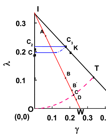
We consider a cubic lattice (size: $L\times L\times L,L=15,20$) with periodic boundary conditions. The biaxial molecules on each lattice site interact through the nearest neighbour interaction potential in Eqn. (1). The parameters $\gamma$ and $\lambda$ are chosen such that we traverse along a trajectory IW passing through the apex I and bisecting the base OV at point W (Fig. 1). The uniaxial - biaxial coupling coefficient $\gamma$ on IW is half of the the value on the diagonal IV, for identical $\lambda$ values. We denote the arclength of the path OIW as $\lambda^{{}^{\prime}}$, given by $\lambda^{{}^{\prime}}=\lambda$ on segment OI, and $\lambda^{{}^{\prime}}=\dfrac{1}{3}(1+5\gamma)$ where $\gamma=\dfrac{(1-3\lambda)}{4}$ on the segment IW. As we traverse along the trajectory IW the arc length $\lambda^{{}^{\prime}}$ varies from $\dfrac{1}{3}$ at I to 0.75 at W. The simulations are done at various values of $\lambda^{{}^{\prime}}$ on the path IW, starting from the point I ($\lambda^{{}^{\prime}}$ = 1/3 at $\gamma$ = 0.0, $\lambda$ = 1/3 ) and ending at W ( $\lambda^{{}^{\prime}}$ = 0.75 at $\gamma$ = 0.25, $\lambda$ = 0.0). Points A ($\lambda^{{}^{\prime}}$ = 0.414 at $\gamma$ = 0.048, $\lambda$ = 0.269), B ($\lambda^{{}^{\prime}}$ = 0.610 at $\gamma$ = 0.166, $\lambda$ = 0.111), $B^{{}^{\prime}}$ ($\lambda^{{}^{\prime}}$ = 0.674 at $\gamma$ = 0.204, $\lambda$ = 0.061) lie in the attractive region for the Hamiltonian, while C ($\lambda^{{}^{\prime}}$ = 0.692 at $\gamma$ = 0.215, $\lambda$ = 0.047) lies on the dispersion parabola and D ($\lambda^{{}^{\prime}}$ = 0.709 at $\gamma$ = 0.225, $\lambda$ = 0.033) lies in the partly repulsive region, below the parabola.

We start the simulation at a chosen value of $\lambda^{{}^{\prime}}$ with a random orientation of spins on the lattice and the corresponding values of $(\gamma,\lambda)$ are inserted in Eqn.1 for calculating the system energy. An entropic ensemble comprising of ($\sim 4\times 10^{7}$) microstates is constructed using the Wang - Landau algorithm, with a fairly uniform distribution of energy at the end of the simulation. Using the DoS computed, canonical ensembles are extracted with reweighting procedure Swensden ; Berg at the chosen temperatures (RW-ensembles). Average values of physical variables are then computed at the required temperature resolution. Information on the system energy and the DoS facilitate the determination of free energy as a function of energy as well as order parameters, at different temperatures.

Conventional MC simulations based on Metropolis algorithm (Boltzmann sampling) leading to equilibrium canonical ensembles (B-ensembles) were also carried out at chosen points on the trajectory IW in order to compare the results from both the simulation methods. These ensembles were collected, after equilibration, with production runs of typically $6\times 10^{5}$ MC lattice sweeps (Monte Carlo steps). Temperature variation of the equilibrium averages from B- and RW-ensembles are compared, to assess the efficacy of the respective sampling in the presence of curious free energy terrains in the configuration space offered by the biaxial system.

The physical observables of interest, calculated at each value of $\lambda^{{}^{\prime}}$, are the average energy $<E>$, specific heat $<C_{v}>$, energy cumulant $V_{4}$ (= $1-<E^{4}>/(3<E^{2}>^{2})$) which is a measure of the kurtosis Binder , the four order parameters of the phase calculated according to Biscarini95 ; Robert and their susceptibilities. These are the uniaxial order $<R^{2}_{00}>$ (along the primary director), the phase biaxiality $<R^{2}_{20}>$, the molecular contribution to the biaxiality of the medium $<R^{2}_{22}>$, and the contribution to uniaxial order from the molecular minor axes $<R^{2}_{02}>$. The averages are computed at a temperature resolution of 0.002 in the temperature ($T^{{}^{\prime}}$) range of interest [2.05, 0.05], all in reduced units. The error bars for the observables were estimated after minimising possible correlations using Jack knife method Newman1 . The relative errors in the averages of energies are found to be typically one part in $10^{5}$, while those in the estimation of the averages of the order parameters are 1 in $10^{4}$.

IV Results and Discussion

We carried out a detailed simulation study employing the entropic sampling technique, at 30 values of $\lambda^{{}^{\prime}}$ with a view to obtaining a generic phase diagram inside $\Delta$ along IW. We examined the temperature dependence of the $C_{v}$ profiles, of the two dominant order parameters $<R^{2}_{00}>$ and $<R^{2}_{22}>$, and the Binder’s energy cumulant $V_{4}$ to determine the phase transition temperatures and identify the phases.

Figure 2: (color online) The temperature variation of order parameters superimposed on the specific heat curves to illustrate the phase behaviour at the four representative point A,B,C and D with values of $\lambda^{{}^{\prime}}$ = (a) 0.414 (Point A) (b) 0.610 (Point B) (c) 0.692 (Point C) and (d) 0.709 (Point D) (L=20)

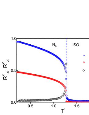
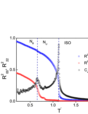
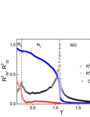
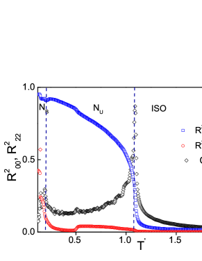
Typical such data at four representative points, at A and B in the fully attractive region, at C on the parabola and at D in the partly repulsive region (Fig. 1), are presented in Fig. 2, with a system size L=20 for point A,B,C and L=15 for point D.

The order profiles superimposed on the specific heat peaks shown in Fig. 2 indicate that a direct isotropic - biaxial phase transition occurs at the point A (Fig. 2). At all other points two specific heat peaks are observed on cooling, at temperatures $T_{1}$ and $T_{2}$. As the system is cooled from the isotropic phase, the uniaxial order $R^{2}_{00}$ shows a sharp increase at $T_{1}$ indicating the onset of an intermediate uniaxial phase phase $N_{U}$. It is of interest to note that this intermediate phase also exhibits a small amount of biaxial order which increases to a value of $\sim$ 0.03, together with the expected significant increase in the uniaxial order as the temperature decreases. The magnitude of $R^{2}_{22}$ in this phase seems to be independent of the $\lambda^{{}^{\prime}}$ value in the attractive region (i.e of the path from I upto C). However on the bordering trajectory between the two distinct regions of the Hamiltonian (i.e point C) and in the partly repulsive region (point D) $R^{2}_{22}$ value actually dips on cooling in this intermediate phase after the initial onset (Figs. 2, 2). The $R^{2}_{22}$ value then increases rapidly at the second transition (at $T_{2}$) for all values of $\lambda^{{}^{\prime}}$, signaling the onset of a low temperature biaxial phase $N_{B}$.

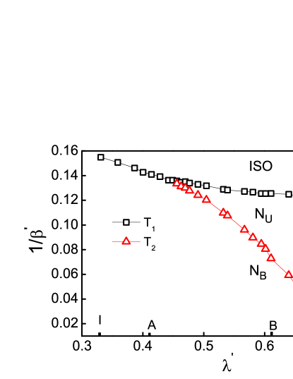
Based on such study along the trajectory IW we obtain the phase diagram, as a function of the arc length $\lambda^{{}^{\prime}}$, shown in Fig. 3. The actual temperature $\textit{T}^{{}^{\prime}}$ of the simulation needed to be scaled by a factor of 9 (for direct comparison with the Lebwohl-Lasher (LL) model LL ), as $\dfrac{1}{\beta^{{}^{\prime}}}=\dfrac{T^{{}^{\prime}}}{9}$.

Figure 3: (color online) Phase diagram inside the essential triangle along path IW

Beyond the value of 0.709 of $\lambda^{{}^{\prime}}$ the parameter region presents dominant cross-coupling term, inducing significant repulsive interactions between the uniaxial and biaxial molecular terms of the neighbouring molecules, thus frustrating the system to find a single, stable and unique free energy minimum. In this scenario, the computational times for the convergence of DoS were found to be impractical at this size (L = 20). We are thus constrained to report data in this region at L=15.

We note from the phase diagram (Fig. 3) that the biaxial medium undergoes a direct $I-N_{B}$ phase transition for $\lambda^{{}^{\prime}}$ values in the range $1/3$ to 0.455. Thereafter, two transitions were observed in the $\lambda^{{}^{\prime}}$ range 0.462 to 0.709. The system undergoes a $I-N_{U}$ transition at the high temperature $T_{1}$, followed by a $N_{U}-N_{B}$ transition at the lower temperature $T_{2}$. It may be seen that the second transition occurs at progressively lower values of $T_{2}$ which approaches zero asymptotically as the point W (on the base OV) is reached, in conformity with the previous MC simulation results in this limit of $\lambda\rightarrow 0$ Luckhurst80 .

Figure 4: (color online) Energy cumulant $V_{4}$ for certain values of $\lambda^{{}^{\prime}}$ in the range 0.345 to 0.692 (point C)

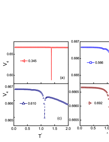
The nature of the transitions can be gleaned from the plots of the fourth order energy cumulant ($V_{4}$) data shown in Fig. 4 for some typical values of $\lambda^{{}^{\prime}}$. The sharp dip in the cumulant value shown in Fig. 4(a) at $\lambda^{{}^{\prime}}$ = 0.345 is indicative of a strong first-order nature of the $N_{B}-I$ transition in the $\lambda^{{}^{\prime}}$ range 0.345 to 0.45. Figs. 4(b) - 4(d) depict the nature of the two transitions in the range of $\lambda^{{}^{\prime}}$ from 0.463 to 0.692. The $I-N_{U}$ transition at $T_{1}$ shows a progressively weakening first order nature (relative to Fig. 4(a)), whereas $N_{U}-N_{B}$ transition seems to be continuous over the trajectory. The trajectory in the repulsive region also shows similar nature of the transitions (Fig. 5).

Figure 5: (color online) Energy cumulant $V_{4}$ for values of $\lambda^{{}^{\prime}}$ in the range 0.709 (Point D) to 0.747 at(L=15)

Figure 6: (color online) Comparison of results obtained from RW ensembles ( hollow black squares) and B ensembles (hollow red circles). Temperature variation of the specific heat(continuous lines) and the order parameter profiles are shown for four values of $\lambda^{{}^{\prime}}$ along the path $IW$: (a)0.566 (b) 0.656 (c) 0.692 (d) 0.709. It is seen that thermal averages of $R^{2}_{22}$ from RW-ensembles differ from the B-ensembles in the intermediate $N_{U}$ phase for values of $\lambda^{{}^{\prime}}>0.566$.

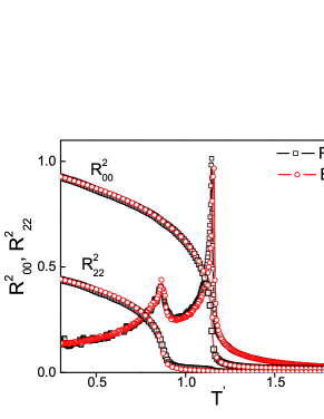
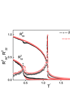
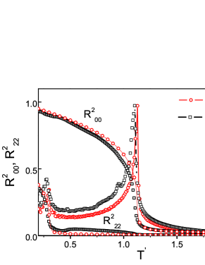
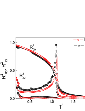
We computed the equilibrium averages of the observables using B-ensembles obtained from MC sampling at randomly chosen points on the trajectory IW. A comparative study of the WL and MC simulation results at four such representative points (at $\lambda^{{}^{\prime}}$ = 0.566, 0.656, 0.692 and 0.709) are shown in Figs. 6 - 6.

It is observed that qualitative agreement exists between the averages computed from RW- and B- ensembles upto (and including) $\lambda^{{}^{\prime}}$ = 0.566. Thereafter the results vary in the behaviour of $R^{2}_{22}$ in the uniaxial phase. While the B-sampling results point to a pure uniaxial phase (i.e $R^{22}_{22}\sim 0$ within the error bars) for all values of $\lambda^{{}^{\prime}}$ along the path IW, the RW-sampling results show an unmistakably non-zero and constant value of $R^{2}_{22}$ ($\sim$ 0.03) in the uniaxial phase for values of $0.566<\lambda^{{}^{\prime}}\leqslant 0.709$.

Figure 7: (color online) Free energy shown as a function of (a) Energy per particle E (b) $R^{2}_{00}$ and (c) $R^{2}_{22}$, on cooling from the isotropic phase to the biaxial phase at $\lambda^{{}^{\prime}}$ = 0.610.

We show the representative free energy plotted as a function of energy (per particle) E and the order parameters $R^{2}_{00}$ and $R^{2}_{22}$ at $\lambda^{{}^{\prime}}$ = 0.610 (point $B^{{}^{\prime}}$) in the attractive region, in Fig. 7, at different temperatures bracketing the two transition points $T_{1}$ and $T_{2}$. We observe that the free energy minima with respect to energy shift towards lower values of energy, while they shift towards higher values of order parameters progressively, as the system is cooled. We also note in Fig. 7(c), that the free energy profile confines the value of $R^{2}_{22}$ to $\sim$ 0.03 in the intermediate temperature region, before allowing its access to higher order values at the onset of $N_{B}$ phase at $T_{2}$. Further, the free energy profile thus confirms that the intermediate phase has to sport in principle a biaxial symmetry, though with a marginal value.

However as we traverse from this fully attractive region of the Hamiltonian towards the dispersion parabola bordering the repulsive region, the free energy profiles with respect the biaxial order display curious deviations, and these persist on entering into the partly repulsive region of the Hamiltonian as well. Fig. 8 compares the temperature dependence of free energy profiles plotted as a function of $R^{2}_{22}$, at different points $B^{{}^{\prime}}$, C, and D in the triangle (Fig. 1). Temperatures are chosen to represent the profiles in different LC phases.

Figure 8: (color online) Representative free energy plotted as a function of $R^{2}_{22}$ for different values of $\lambda^{{}^{\prime}}$ : (a) 0.674 (b) 0.692 and (c) 0.709 (L=20 for (a) and (b) and L=15 for (c).

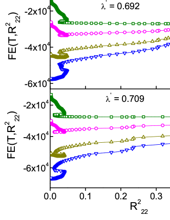
We note from Fig. 8(a) that the free energy curves at $\lambda^{{}^{\prime}}$ = 0.674 (point $B^{{}^{\prime}}$) show shallow minima at finite values of $R^{2}_{22}$ (ranging from 0.03 in the $N_{U}$ phase to 0.24 at the onset of the $N_{B}$ phase). In contrast free energy curves at $\lambda^{{}^{\prime}}$ = 0.692 (Fig. 8(b) at point C located on the parabola) and 0.709 (Fig. 8(c) at point D, in the partly repulsive region) show a rather unusual behaviour in $N_{U}$ phase, however consistent with the temperature dependence of the observed average values of $R^{2}_{22}$, i.e initial increase to a higher value at the onset of $N_{U}$ phase and subsequent dip on cooling just before the onset of $N_{B}$ phase.

Noting the established accord between the temperature variation of average values of order parameters and the corresponding free energy profiles in this parameter region, and also keeping in view the observation that the free energy on the other hand shows a smooth variation with the energy of the system, the obvious pointer is to suggest subtle changes in the relative contributions of the different orders to the entropy of the system. It seems to show rather pointedly that in the neighbourhood of the parabolic boundary, the increased contribution of the cross-coupling term ($\gamma$), at the expense of the biaxial-biaxial coupling ($\lambda$) attempting to promote macroscopic molecular biaxial order, do not leave the intermediate unixial phase in its pristine form (compared to, say, the nematic phase in LL-model or even in the biaxial system on the $\lambda$-axis, for example). It may be noted that the presence of such inhomogeneous structures and their contribution to the macroscopic averages of order have been investigated and the presence of ’clusters’ was alluded to, in the biaxial cluster model of nematics by Vanakaras Vanakaras08 ; Vanakaras09 , (which was proposed to explain the recent experimental observation of phase baixiality in bent-core nematics). Indeed this specific uniaxial phase seems to host local inhomogeneties catering to increased $\gamma$ contribution and thus shows a non-zero macroscopic $R^{2}_{22}$ initially originating from such clusters. The subsequent decrease of biaxial order on further cooling in the uniaxial phase appears to be an indication of the increasing role of primary order parameter $R^{2}_{00}$ in effectively contributing to the free energy minimization in the process making the system perhaps a more homogeneous uniaxial medium.

Figure 9: (color online) Correlation function G(r) of x,y and z molecular axes plotted as a function of the distance r at the point C ($\lambda^{{}^{\prime}}$ = 0.692 ) at two temperatures in the $N_{U}$ phase.

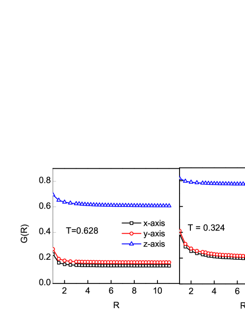
Taking advantage of the non-monotonic variation of $R^{2}_{22}$ within the $N_{U}$ phase at the point C (on the parabola), we chose two temperature points (0.628 and 0.324) at which the average value of $R^{2}_{22}$ are the same (Fig. 2). We collected microstates within a narrow range centered at the corresponding average energy values per site (-2.331 $\pm$ 0.001, -2.784 $\pm$0.001 respectively), constituting effectively microcanonical ensembles located at the most probable energy values at the respective temperatures. We computed the orientational correlations of different molecular axes with distance (in lattice units), to obtain their spatial correlation functions at the two temperatures. These variations are shown in Fig. 9. Obviously $R^{2}_{00}$ has increased significantly over this temperature range and is reflected in the long-range correlation values of the z-axes. The minor axes (x and y) however have qualitatively different decays, flattening to two different plateau values, even though the corresponding macroscopic averages of $R^{2}_{22}$ are chosen equal. This clearly brings out the subtle differences in the microscopic organization in the two biaxial phases at the two temperatures: the low temperature phase hosts a higher long-range $R^{2}_{00}$ order as expected, but interestingly also a relatively higher long-range $R^{2}_{22}$ order. It may also be seen from the initial decay profiles of the minor axes at the low temperature (Fig. 9), that this hosts biaxial clusters which are correlated over larger range than their counterparts at the high temperature point. The low temperature phase seems to correspond to an emerging homogeneous biaxial phase, homogeneity being perhaps imposed through free energy considerations, by the inherent degree of the dominant uniaxial order $R^{2}_{00}$. The fact that these two temperatures had the same macroscopic $R^{2}_{22}$ order, despite having qualitatively differing correlation profiles, also confirm the presence of contributions to $R^{2}_{22}$ possibly arising from geometrical averages over inhomogeneous regions, at high temperature.

IV.1 Study along the parabolic path OT

The parabolic path within the triangle extends from the origin O ($\gamma$ = 0, $\lambda$ = 0, corresponding to the LL model) to the Landau point T ($\gamma=1/3$, $\lambda=1/9$) and the interaction parameters are related within the dispersion approximation as $\lambda=\gamma^{2}$. We carried out entropic sampling based MC study at 13 closely spaced points on the parabola (excluding the origin) and the observed that phase sequence remained the same $I-N_{U}-N_{B}$ at all points except at T. The Landau point was found to be qualitatively different, hosting two distinct biaxial phases instead, as reported in a recent entropic sampling based MC study Kamala14 ; Kamala15 . It may be noted that this finding however differs from the mean field prediction Freiser ; Alben ; Bisi06 as well as MC reults from Boltzmann sampling Biscarini95 . The latter studies point to a single low temperature $N_{B}$ phase after a direct transition from the isotropic phase.

Figure 10: (color online) Uniaxial order ($R^{2}_{00}$) and biaxial order ($R^{2}_{22}$) plotted as a function of reduced temperature for values of $\gamma$ ranging from (a) 0.131 - 0.228 (b) 0.245 - 0.333. Inset in (a) shows a magnified version of the $R^{2}_{22}$ vs $T$ plot where the decrease of $R^{2}_{22}$ at lower temperatures is seen.

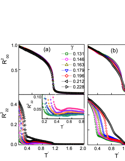
We present the order parameter profiles at various points on the parabola starting from $\gamma$ = 0.131 to $\gamma=1/3$ in Fig. 10 (at L = 20). It is observed from Fig. 10(a) that the biaxial order parameter shows an initial small increase at the onset of the $I-N_{U}$ transition, followed by a decrease in its value in the deeper uniaxial nematic phase. This anomalous behaviour is more pronounced for values of $\gamma$ ranging from 0.163 - 0.212. The $R^{2}_{22}$ temperature profiles for $\gamma$ values in the range 0.245 - 0.333 on the other hand, increase continuously in the $N_{U}$ phase (Fig. 10(b)) exhibiting a monotonic behaviour. It is observed from both the graphs that the temperature range of the uniaxial nematic phase decreases and biaxial phase appears at progressively higher temperatures, as the $\gamma$ value increases along the parabola. A curious observation from this study is that the intermediate $N_{U}$ phase is not strictly uniaxial with $R^{2}_{22}$ = 0 (as expected from the earlier studies), but hosts a small degree of biaxial order in the intermediate temperature range. This feature becomes prominent as $\gamma$ value increases beyond $\sim$ 0.2, indicating the increasingly competing role of the cross-coupling interaction on this very special boundary.

Figure 11: (color online) Free energy plotted as a function the biaxial order parameter $R^{2}_{22}$ for four values of $\gamma$ in the neighbourhood of point C (including C, $\gamma$ = 0.212)

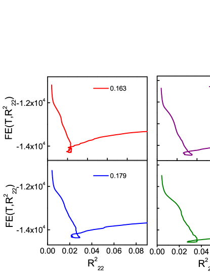
The free energy profiles (plotted against $R^{2}_{22}$) shown in Fig. 11 at temperature T = 0.5 for values of $\gamma$ between 0.163 and 0.212 on the parabola, show the presence of loop like structures, similar to the earlier observations at point C (Fig. 8(b)), and consistent with the temperature variation of average $R^{2}_{22}$ values.

Figure 12: (color online) Free energy shown as a function of $R^{2}_{22}$, on cooling in the uniaxial nematic phase for values of $\gamma$ = (a) 0.228 (b) 0.294 (c) 0.333

For higher values of $\gamma$ (0.228 - 0.333, Fig. 12) however, these show variations on cooling, which are in accord with the behaviour of $R^{2}_{22}$ in this region of the parabola.

Thus it emerges, that the intermediate $N_{U}$ phase hosts distinct molecular organizations as the medium is transformed in terms of the symmetry of its molecular interactions from LL - model to the Landau point along the parabola. Discernible degree of biaxial order and its curious temperature variations along the path starting from the origin (LL model) hint at the possibility that the parabola is in fact a very special trajectory having differing types of $N_{U}$ phases as the Landau point is reached. The parabola at once serves both as an interesting boundary between distinct natures of the Hamiltonian, as well as transforms the system interaction symmetry while simultaneously promoting the influence of the cross-coupling terms, as one moves over from the LL limit. Obviously non-monotonic temperature dependence of $R^{2}_{22}$ is associated with complex free energy terrain exhibited by the system in the $R^{2}_{00}$ - $R^{2}_{22}$ space, originating from increasing degree of cross-coupling term. Viewed from this perspective, the present data provide an insight into the role of $\gamma$ and $\lambda$ as their relative importance changes on this trajectory.

V Conclusions

We report the results of detailed MC simulations (based on Wang - Landau technique) along two trajectories inside the triangle $\Delta$. In the first case, along the line IW, we find that our results are in accord with MF predictions in terms of the phase sequences expected. We observe however that as we progressively move towards the base point W, in the process changing the relative importance of $\gamma$ and $\lambda$ terms in Eqn. 1, the uniaxial phase develops a marginal degree of biaxial order $R^{2}_{22}$ which is sustained through the uniaxial range. This is similar to our earlier observation on the diagonal IV as one progressively traverses towards V Kamala14 ; Kamala15 . The onset of a biaxial phase with significant order at the low temperature transition is preceded by a dip in $R^{2}_{22}$ from its small value ($\sim$ 0.03).

The trajectory IW encompasses two distinct regions from the point of view of nature of the Hamiltonian. Upto the point C where IW intersects the dispersion parabola, H is fully attractive. The segment CW corresponds to a partly repulsive region, making the stability of the biaxial phase untenable asymptotically as the point W is reached. We make use of the DoS estimates in our simulation to plot the free energy profiles as function of order parameters ($R^{2}_{00}$ , $R^{2}_{22}$) as well as energy. The observed interesting temperature variation of $R^{2}_{22}$ within the ’uniaxial’ phase is consistent with the requirements of the free energy profiles at different $\lambda^{{}^{\prime}}$ values along the trajectory.

The parabolic trajectory OCT, very well studied earlier for its simplifying dispersion approximation, is revisited with the present MC technique to examine if the intermediate uniaxial phase retains its pristine symmetry ($R^{2}_{22}$ = 0 in this phase) throughout its path. The present data indicate that the intermediate uniaxial phase exhibits a small degree of biaxial order as $\gamma$ increases, and as Landau point is reached it indeed seems to transform into a biaxial phase in its own right Kamala14 ; Kamala15 .

The appearance of a small degree of biaxial symmetry within the uniaxial phase, whenever $\gamma$ assumes a dominant role, has its origin in the presence of local biaxial inhomogeneities (referred to as ’clusters’ in Vanakaras08 ; Vanakaras09 ). Their formation and sustenance is facilitated by the corresponding cross-coupling interaction which eventually interferes with the homogeneous onset of the two orders. This inference may well have implications in the observed difficulties in realizing readily a biaxial phase in the laboratory.

VI Acknowledgments

We wish to thank Surajit Dhara, School of Physics, University of Hyderabad for useful discussions. The simulations were carried out in the Centre for Modelling Simulation and Design (CMSD) at the University of Hyderabad. BKL acknowledges financial support from Department of Science and Technology, Government of India vide grant ref No: SR/WOS-A/PM-2/2016 (WSS) to carry out this work.

References

- (1) M. J. Freiser, Phys. Rev. Lett. 24 , 1041 (1970).
- (2) J. P. Straley, Phys. Rev. A. 10, 1881 (1974).
- (3) R. Alben, Phys. Rev. Lett. 30, 778 (1973).
- (4) G. R. Luckhurst, C. Zannoni, P. L. Nordio and U. Segre, Mol. Phys. 30, 1345 (1975).
- (5) N. Bocara, R. Mejdani and L. De Seze, J. Phys. (Paris) 38, 149 (1976).
- (6) E. F. Gramsbergen, L. Longa and W. H. de Jeu, Phys. Rep. 135, 195 (1986).
- (7) D. K. Remler and A. D. J. Haymet, J. Phys. Chem. 90, 5426 (1986).
- (8) Bela Mulder, Phys. Rev. A., 39, 360 (1989).
- (9) P. I. C Teixeira, A. J. Masters and B. M. Mulder, Mol. Cryst. Liq. Cryst. Sci. Technol., Sect. A, 323, 167 (1998).
- (10) B. R. Acharya, A. Primak and S. Kumar, Phys. Rev. Lett. 92, 145506 (2004).
- (11) L. A. Madsen, T. J. Dingemans, M. Nakata and E. T. Samulski, Phys. Rev. Lett. 92, 145505 (2004).
- (12) K. Merkel, A. Kocot, J. K. Vij, R. Korlacki, G. H. Mehl and T. Meyer, Phys. Rev. Lett. 93, 237801 (2004).
- (13) J. L. Figueirinhas, C. Cruz, D. Filip, G. Feio, A. C. Ribeiro, Y. Frere, T. Meyer and G. H. Mehl, Phys. Rev. Lett. 94, 107802 (2005).
- (14) K. Severing and K. Saalwachter, Phys. Rev. Lett. 92, 125501 (2004).
- (15) G. R. Luckhurst and S. Romano, Mol.Phys. 40, 129 (1980).
- (16) M. P. Allen, Liq. Cryst. 8, 499 (1990).
- (17) F. Biscarini, C. Chiccoli, P. Pasini, F. Semeria, and C. Zannoni, Phys. Rev. Lett. 75, 1803 ( 1995).
- (18) P. J. Camp and M. P. Allen, J. Chem. Phys. 106, 6681 (1997).
- (19) C. Chiccoli, P. Pasini, F. Semeria, and C. Zannoni, Int. J. Mod. Phys. C 10, 469 (1999).
- (20) S. Romano, Physica A 337, 505 (2004).
- (21) S. Romano, Physica A 339, 511 (2004).
- (22) G. Sai Preeti, K. P. N. Murthy, V. S. S. Sastry, C. Chiccoli, P. Pasini, R. Berardi and C. Zannoni, Soft Matter 7, 11483 (2011).
- (23) B. Kamala Latha, Regina Jose, K. P. N. Murthy and V. S. S. Sastry, Phys. Rev. E 89, 050501(R) (2014).
- (24) B. Kamala Latha, Regina Jose, K. P. N. Murthy and V. S. S. Sastry, Phys. Rev. E 92, 012505 (2015).
- (25) K. Van Le, M. Mathews, M. Chambers, J. Harden, Quan Li, H. Takezoe and A. Jakli, Phys. Rev. E 79, 030701 (R) (2009).
- (26) N. Vaupotic, J. Szydlowska, M. Salamonczyk, A. Kovarova, J. Svoboda, M. Osipov, D. Pociecha and E. Gorecka, Phys. Rev. E 80, 030701 (R) (2009).
- (27) Mamatha Nagaraj, Y. P. Panarin, U. Manna, J. K. Vij, C. Keith and C. Tschierske. Appl. Phys. Lett. 96, 0111106 (2010).
- (28) A. M. Sonnet, E. G. Virga, and G. E. Durand, Phys. Rev. E 67, 061701 ( 2003).
- (29) Lech Longa, P. Grzybowski, S. Romano and E. Virga, Phy. Rev. E 71, 051714 (2005).
- (30) G. De Matteis, and E. G. Virga, Phys. Rev. E 71, 061703 (2005).
- (31) G. De Matteis, S. Romano and E. G. Virga, Phy. Rev. E 72, 041706 (2005).
- (32) F. Bisi, E. G. Virga, E. C. Gartland Jr., G. De Matteis, A. M. Sonnet, and G. E. Durand, Phys. Rev. E 73, 051709 (2006).
- (33) G. De Matteis, F.Bisi and E. G. Virga, Continuum Mech. Thermodyn. 19, 1 - 23 (2007).
- (34) G. De Matteis and S. Romano, Phys. Rev. E, 78, 021702 (2008).
- (35) P. A. Lebwohl and G. Lasher, Phys. Rev. A 6, 426 ( 1972).
- (36) F. Bisi, G. R. Luckhurst and E. G. Virga, Phys. Rev. E 78, 021710 (2008).
- (37) R. Berardi and C. Zannoni, J. Chem. Phys. 113, 5971 (2000).
- (38) C. Chiccoli, I. Feruli, O. D. Lavrentovich, P. Pasini, S. V. Shiyanovsiccoli1kii and C. Zannoni, Phys. Rev. E 66, 030701 (2002).
- (39) C. Chiccoli, P. Pasini, I. Feruli and C. Zannoni, Mol. Cryst. Liq. Cryst. 441, 319 (2005).
- (40) R. Berardi, L. Muccioli and C.Zannoni, J. Chem. Phys. 128, 024905 (2008).
- (41) R. Berardi, L. Muccioli, S. Orlandi, M. Ricci and C. Zannoni, J. Phys.: Condens. Matter. 20, 463101.1 (2008).
- (42) F. Wang and D. P. Landau, Phys. Rev. Lett. 86, 2050 (2001); F. Wang and D. P. Landau, Phys. Rev. E 64, 056101 (2001).
- (43) D. P. Landau and K. Binder, A Guide to Monte Carlo Simulations in Statistical Physics, Cambridge University Press, 2nd edition(2005).
- (44) K. P. N. Murthy, Monte Carlo Methods in Statistical Physics Universities Press, India(2004).
- (45) N. Rathore, T. A. Knotts and J. J. de Pablo, Biophysics. J. 85, 3963 (2003).
- (46) D. T. Seaton, T. Wust and D. P. Landau, Phys. Rev. E 81, 011802 (2010).
- (47) Priya Singh, Subir. K. Sarkar and Pradipta Bandyopadhyay, Chem. Phys. Lett. 514, 357 (2011).
- (48) Lili Gai, Thomas Vogel, Katie A. Maerzke, Christopher R. lacovella, David P. Landau, Peter T. Cummings and Clare McCabe, J. Chem. Phys. 139, 054505 (2013).
- (49) P. Poulain, F. Calvo, R. Antoine, M. Broyer and P. Dugourd, Phys. Rev. E 73, 056704 (2006).
- (50) S. Sinha and S. K. Roy, Phys. Lett. A 373, 308 (2009).
- (51) Raj Shekhar, Jonathan K. Whitmer, Rohit Malshe, J. A. Moreno-Razo, Tyler F. Roberts and Juan J. de Pablo, J. Chem. Phys. 136, 234503(2012).
- (52) Yang Wei Koh and Hwee Kuan Lee, Phys. Rev. E 88, 053302 (2013).
- (53) Thomas Vogel, Ying Wai Li, Thomas Wust and David. P. Landau, Phys. Rev. Lett. 110, 210603 (2013).
- (54) Katie A. Maerzke, Lili Gai, Peter T. Cummings and Clare McCabe, J. Phys. Conference Series 487, 012002 (2014).
- (55) Y. L. Xie, P. Chu, Y. L. Wang, J. P. Chen, Z. B. Yan, J .M. Liu, Phys. Rev. E 89, 013311 (2014).
- (56) D. Jayasri, V. S. S. Sastry, and K. P. N. Murthy, Phys. Rev. E 72, 036702 (2005).
- (57) C. Zhou, T. C. Schulthess, S. Torbrugge, and D. P. Landau, Phys. Rev. Lett. 96, 120201 (2006).
- (58) D. Jayasri, Ph. D Thesis, Non-Boltzmann Monte Carlo study of Confined Liquid Crystals and Liquid Crystal Elastomers, University of Hyderabad, India(2009).
- (59) R. H. Swendsen and J. S. Wang, Phys. Rev. Lett. 58, 86 (1987).
- (60) B.A. Berg, cond-mat. 0206333.
- (61) K. Binder, Z. Physik. B 43, 119 (1981); K. Binder, Phys. Rev. Lett. 47, 693 (1981).
- (62) Robert J Low, Eur. J. Phys. 23, 111 ( 2002).
- (63) M. E. J. Newman and G. T. Barkema, Monte Carlo Methods in Statistical Physics , Clarendon Press, London(2002).
- (64) A.G. Vanakaras and D. J. Photinos. J. Chem. Phys. 128,154512 (2008).
- (65) S.D. Peroukidis, P. K. Karahaliou, A. G. Vanakaras and D. J. Photinos, Liq.Cryst. 36:6, 727 (2009).