Current address:]Hampton University, Hampton, VA 23668 Current address:]University of Dammam College of Education of Jubail Department of Physics P.O 12020, Industrial Jubail 31961 Saudi Arabia
The CLAS Collaboration
Measurement of the Differential and Total Cross Sections of the Reaction within the Resonance Region
Abstract
We report the first measurement of differential and total cross sections for the reaction, using data from the CLAS detector at the Thomas Jefferson National Accelerator Facility. Data collected during two separate experimental runs were studied with photon-energy coverage GeV and GeV, respectively. The two measurements are consistent giving confidence in the method and determination of systematic uncertainties. The cross sections are compared with predictions from the KAON-MAID theoretical model (without kaon exchange), which deviate from the data at higher and at forward kaon angles. These data, along with previously published cross sections for photoproduction, provide essential constraints on the nucleon resonance spectrum. A first partial wave analysis has been performed that describes the data without the introduction of new resonances.
I Introduction
New states have been discovered in the spectrum of nucleon resonances in recent years, which are summarized by the Particle Data Group (PDG) Patrignani et al. (2016), in part due to high-precision data from photon-beam facilities, and also due to theoretical advances in coupled-channel partial wave analyses Anisovich et al. (2012). Some nucleon resonances, or ’s, have a weak coupling to final states yet may have significant branching ratios to final states with strangeness, such as . Most of the strangeness photoproduction data comes from reactions using a proton target. However, protons and neutrons have different photocouplings to the ’s and measurements of cross sections off the neutron give complementary information Close (1979). Here, we present the first measurements of the reaction where the proton is a spectator. (In fact, the proton can contribute in some kinematics through final-state interactions, but based on results of other analyses we expect these effects to be small here Zachariou (2017).) One advantage of studying this reaction is that the is an isosinglet, and hence only resonances (and no resonances) can contribute to -channel diagrams, thus simplifying the theoretical interpretation of the data.
The measurements are compared with theoretical predictions from an approach that is based on a unitarized tree-level Lagrangian model Mart et al. (2000). The model includes phenomenological couplings of ’s to the final state, based on fits to existing kaon production data McCracken et al. (2010); Bradford et al. (2006); McNabb et al. (2004), with photocouplings to the ’s extracted from previous measurements (more in Section IV.1). The calculations also include -channel exchange based on the Regge model. Since the has no charge or spin, the -channel contributions to photoproduction only come from an exchange of a strange meson with spin , such as a .
A comparison between the data and theoretical predictions will allow us to obtain information on which ’s contribute to this reaction. In particular, there are many resonances predicted by the constituent quark model Koniuk and Isgur (1980); Capstick and Roberts (1998) or by lattice gauge theory Edwards et al. (2013) that are not seen in experiments and are commonly referred to as “missing” resonances. Recent work by the Bonn-Gatchina group Anisovich et al. (2012) has added a few new resonances, but many are yet to be observed.
At lower center of mass energies, , only , , and were predicted to contribute significantly to production. However, the SAPHIR Tran et al. (1998); Glander et al. (2004) and CLAS McCracken et al. (2010); Bradford et al. (2006); McNabb et al. (2004) photoproduction data off a proton target show an enhancement at GeV. Partial Wave Analyses (PWA) suggested that this corresponds to a new resonance, the , which couples only weakly to final states Anisovich et al. (2012). Given these findings, data utilizing photoproduction off the neutron are very important to understand these resonant states. The measurement of the cross sections is expected to lead to the determination of excitation coupling strengths, relative to the proton.
II The Experiments
The g10 and g13 datasets were collected using the CEBAF Large Acceptance Spectrometer (CLAS) at the Thomas Jefferson National Accelerator Facility. The experiments used a tagged Bremsstrahlung photon beam Sober et al. (2000) created from the primary electron beam of the CEBAF accelerator. These photons were tagged by determining the scattered electron energy Sober et al. (2000). This allowed tagging photons between 20% and 95% of the incident electron energy () with resolution of .
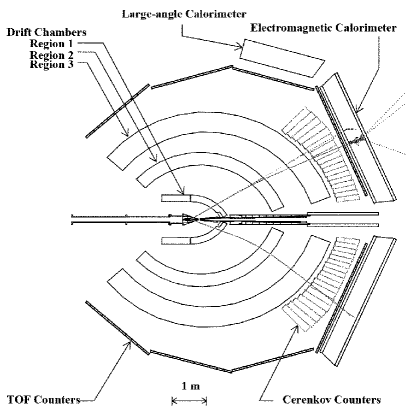
Some of the generated photons interacted with the liquid deuterium target and produced a neutral and a baryon. Each of the final state hadrons decayed into pions and a proton that were tracked by the drift chambers Mestayer et al. (2000) in a toroidal magnetic field Mecking et al. (2003) to determine the charge and momenta of the particles. The time-of-flight was determined using the start counter Taylor et al. (2001); Sharabian et al. (2006), surrounding the target, and the (stop) counters on the exterior of CLAS Mecking et al. (2003). A schematic of CLAS can be seen in Fig. 1. The detected particles were then used to reconstruct the momenta and trajectories of the produced kaon and in the offline analysis.
II.1 g10 Experiment
The g10 experiment directed the CEBAF electron beam onto a gold foil to produce an unpolarized bremsstrahlung photon beam, which then struck an unpolarized liquid-deuterium target. The target chamber was conical, measuring 24 cm in length with a maximal diameter of 4 cm. The center of the target was positioned 25 cm upstream from the CLAS center. For this experiment the incident electron energy was 3.767 GeV, which allowed a maximum tagged photon energy of about 3.6 GeV.
The analysis on this dataset was limited to photon energies between 1.0 GeV and 3.0 GeV where event rates were the largest. The torus had two different current settings, +2250 A and +3375 A Chen et al. (2009). Each magnet setting was kept for roughly half of the g10 beam time. The positive polarity, which bends negatively charged particles towards the beamline, combined with the high torus setting, resulted in some low-momentum tracks curling far enough inward to never be seen by the time-of-flight (stop) counters. Therefore, this analysis only investigated the data set with the torus magnet set at +2250 A as to increase the probability of detecting lower momentum ’s.
II.2 g13 Experiment
This analysis used the g13 experiment’s data with circularly polarized photons that were generated using a polarized electron beam at an energy of 2.65 GeV. The torus magnet current was set to A to have larger efficiency for low momentum ’s that bent away from the beamline, in contrast to g10’s positive torus polarity. A conical 40-cm-long unpolarized liquid-deuterium target was used during the g13 experiment. This was positioned 20 cm upstream from the CLAS center with a maximal diameter of 4 cm. This set-up was intended to maximize the acceptance of low-momentum ’s that resulted from the decays of hyperons. These data were used for the cross section determination presented here due to its large energy overlap with the g10 data set.
III Data Analysis
The different run conditions of the g10 and g13 experiments allowed a check on the reproducibility of this first cross section measurement. Differences in these independent measurements include the photon tagger energy range, photon flux, and torus field strength and polarity.
III.1 Particle Identification
The short lifetime and neutral charge of the reaction products of interest, and , make their direct detection virtually impossible. The particles were reconstructed through their decays: and . Having no particles detected directly from the reaction vertex required an extra step to determine the decay vertex, which was used to account for energy losses due to ionization (and momentum corrections). These corrections are essential for making a direct and reliable comparison of data and simulation.
The final-state particles representing the reaction of interest are three pions and a proton. Particle identification consisted of a comparison between the measured time-of-flight, , and the calculated time using the particle’s assumed mass and momentum (as extracted from tracking);
| (1) |
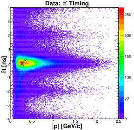
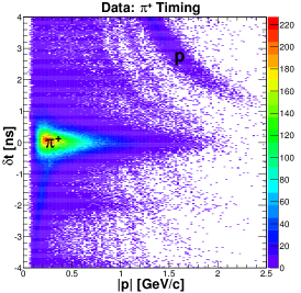
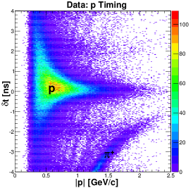
where is the reconstructed path length of the particle from the event vertex to the TOF counters, is the assumed mass of the particle, and is the time-of-flight as calculated by taking the difference between the TOF time and the event start time. Particle identification was performed separately for positive and negative tracks. Fig. 2 shows a very small subset of the raw g13 data, in which is determined for each track, given its measured quantities (, charge, and momentum) for assumed masses of a and . The time difference about was fit as a function of momentum with a Gaussian for several momentum bins; a () cut about the centroid of was used to identify particles in g13 (g10) data. Fig. 2 shows horizontal bands at ns and ns that reflect the 2 ns RF period of the CEBAF electron beam.
III.2 Event Selection
Once the candidate events with all the required particles were identified, their tracks were paired to reconstruct the possible and particles. The decays 69% of the time into a pair Patrignani et al. (2016), while the has a 64% branching ratio to the channel Patrignani et al. (2016). It cannot be certain apriori which of the two ’s was the partner of the proton and which one of the , so each combination was considered. The pair that yielded an invariant mass closest to the mass was chosen. From both simulation and data studies, it was shown that less than 1.0% of surviving events were then paired incorrectly Compton et al. (2014, 2016). This showed that each could be reliably assigned to a corresponding or (when a event existed) and was used for and reconstruction in this analysis.
Several corrections and cuts were applied before the final yield extraction was done. The momenta of the tracks was corrected for the energy lost as the particles passed through the target and start counter Pasyuk (2007). Slight corrections were also necessary for the momentum of each track, due to uncertainties in the magnetic field, and for the tagged photon energy, caused by the sag of the tagger focal plane McCracken et al. (2010). Cuts were also made to remove poorly performing tagger counters and time-of-flight paddles. Events associated with beam trips were also cut from the final analysis.
Every particle that traverses through CLAS can be described by its production vertex, momentum (), and mass. To increase reliability, all tracks that were reconstructed close to the edges of the detector were removed from both data and simulation McCracken et al. (2010). These trajectories were identified based on the decrease in the number of reconstructed particles in finite bins of the vertex, momentum (), and mass. These fiducial cuts change with each experiment, due to different magnetic fields and target locations.
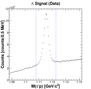
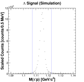
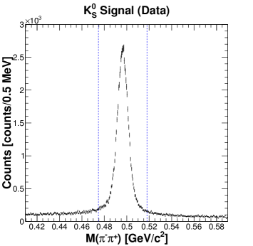
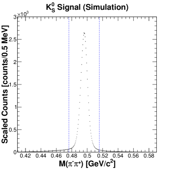
Figures 3 and 4 show the reconstructed invariant mass distributions of and , respectively. One can clearly see the and peaks. The peaks sit on top of background, which was mostly due to non-resonant production. The phase space background can be reduced by a cut on the opposing particle’s ( or ) mass distribution (a 4 cut was used in this analysis). To illustrate that the data has peaks where they are expected, a simulation of was compared with the data. At this point the data contained a large amount of background. To reduce this background, cuts on the invariant mass (as discussed above) were imposed on the data and simulation. The peak location, width of these signal peaks, and a representation of where a 4 cut would lie is shown in Fig. 3 and 4 for the reconstructed and , respectively.
III.3 Yield Extraction
Extraction of the exclusive events from the sample of events requires the background contributions to be identified and removed (or accounted for). Also, final-state-interaction events need to be eliminated or strongly suppressed. Previous studies of the reaction of interest Nadel-Turonski et al. (2006) have shown that the distribution of the missing mass off the kaon, (where was assumed to be at rest), versus the missing mass off , , was useful in understanding background contributions from reactions with higher-mass hyperons such as and . This can be seen in Fig. 5.
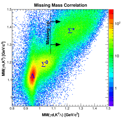
The events of interest yield a peak in at the mass. This peak was much wider, compared to production off the free proton, since the Fermi momentum of the target neutron was not taken into account in the calculation of . This quantity, due to the undetected nucleon, was not sufficient to remove background. While the cannot be removed with a simple cut, the contributions can be reduced to a negligible amount by removing all events with GeV/c2. This means the signal does not extend underneath the peak when working with the projection onto . A similar argument was made for , or other events with a missing pion. Therefore, was used for the yield extraction as discussed throughout this document.
The distributions in Fig. 6 illustrate the missing mass after cuts on the invariant mass of the and . Although much background remains, it is clear where the corresponding signals from the and reactions are located. The later cuts on missing mass and missing momentum remove any significant contribution from events associated with the production of an extra (or ) such as in the case of the higher-mass hyperons and or higher-mass kaons. The yield for can be determined by fitting the missing proton peak after the analysis cuts. To do this the background shape must be understood. Fitting the full spectrum of both the proton peak (corresponding to the missing mass of the ) and the proton plus photon peak () was problematic due to the overlap of these signals.
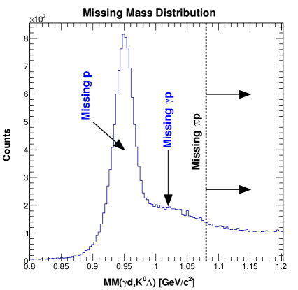
To extract a more reliable yield, the fitting of was approached by means of only describing the leading edge of the distribution. Generated data allowed a very good approximation of background contributions, and these were used to perform background subtraction as described in the next section. Specifically, the shape of the background was determined by fitting the simulated spectrum after it was processed through the modeled detector. This shape was then scaled to match the distribution of our actual data. The yields were extracted by the integration of the signal and by scaling the background shapes to the data.
III.4 Background
The reaction of interest was . To measure this process the decay products of the and were detected. Therefore the final state particles that were detected were . The four tracks could be produced several different ways. The backgrounds can be attributed to two categories. The first category was a five (or more) track background, where one (or more) tracks were missed by CLAS. The second category of background processes was from a four track background.
III.4.1 Hyperon Backgrounds
By extracting the yield through the missing mass, it was likely that any process producing an extra pion (or other massive particle) was well separated from the spectator proton missing mass measured by , where is the four-momentum of the given particle. Near the missing mass signal the most prevalent five track background was identified as . Nonetheless other background channels were also explored.
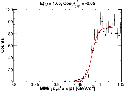
The background could not be separated from the signal except through the missing mass, as this still produced a peak at the and invariant masses. The characteristic shape of this background was explored through simulation. When extracting the yield for the channel, a fit to this background shape was used to subtract the events, which can be seen in Fig. 7. Simulation showed that the edge of the distribution consistently resulted in a sigmoidal shape. Several fitting functions (with sigmoidal properties) proved reasonably consistent, yet the hyperbolic tangent function proved most reliable in estimating the events under the proton missing mass distribution. Momenta of the missing particles was not used to separate the background but is discussed in Section III.6. This background combined with simulated events represented the data fairly well. Other five track backgrounds that do not produce real ’s or ’s were significantly reduced by the invariant mass cuts and separated from the signal by a large missing mass.
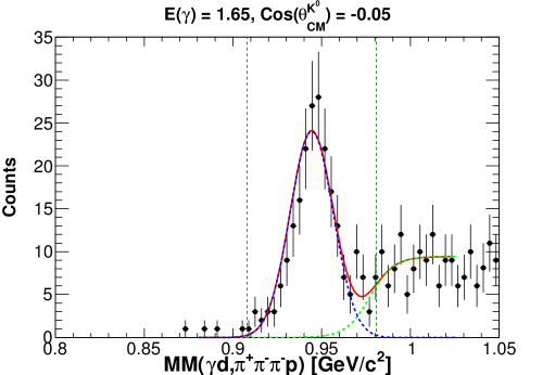
Other hyperon backgrounds were studied using simulations of detector acceptance. An equal number of events was generated for the channel and the two lowest energy competing background channels - the and channels. Phase space was used for the event generation. There was a negligible contribution of both channels, which reflected their extremely low acceptance. This, combined with the improbability that the missing mass was near the spectator proton mass, suggests that these channels were not contaminating the dataset.
III.4.2 Four Track Background
While the strange channels (such as and ) were the primary source of our four final state particle events, other processes from non-strange production mechanisms could contribute to the background. One to consider is the production channel of . Both the and have a wide mass distribution when compared to either the or peaks. When this channel is considered it could easily produce a relatively broad distribution about the invariant masses of the and . Likewise if there were other similar background processes, the general trend would be creating a missing mass peak at the value of the proton mass, but would not produce a peak at the kaon or mass.
Regardless of the channel, one would expect scattering events where the final state particles were directly produced from photon-nucleon interactions. In this case, the background from is expected. Because there were multiple channels contributing to the background, they were modeled with simulations. This “random” distribution resulted with kinematics filling in the phase space underneath the signal peaks ( and ). A uniform phase space distribution was generated to model this background. Although most of the generated phase space events were not in the region of interest, the events that did pass the limiting cuts matched the background shape under the signal and the signal.
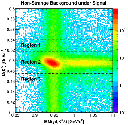
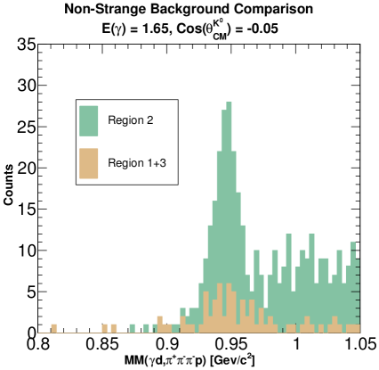
To account for this background, the sidebands of were projected onto the missing mass plane, where by definition this background created a peak at the spectator proton mass. The number of events that were only missing a spectator proton were found in each region noted in Fig. 8. To obtain the correct number of events, subtraction was used based on the sidebands of the distribution. The events in Region 2 of Fig. 8 can be written as
| (2) |
where is the number of events, is the number of events, and is the number of events that do not follow from the decays of or . To correct for the overestimates of yield, events in Region 1 and Region 3 of Fig. 8,
| (3) |
were subtracted from the events of Region 2. The size of this background fluctuated near 15% depending on the kinematic bin. This resulted in the raw yield of after subtraction of events.
III.5 Photon Flux
Photons incident on the target were tallied and then corrected by the tagger efficiency as they were written into the flux files Ball and Pasyuk (2005). The analysis code then cycled through the files to sort photons into the same energy bin structure as the yield extraction. Events without a corresponding photon flux file were dropped from the analysis. Analysis was performed on the consistency of the yield-to-flux ratio, or normalized yield. This generated an estimate of stability for each run within the experiment. Most energies showed a variation less than 3% in the normalized yield for g13 and less than for g10. This uncertainty was accounted for in the calculation of the luminosity uncertainty for the cross section (see Tables 1 and 2).
III.6 Monte Carlo Simulation
Monte Carlo simulation was used to determine the true acceptances in the CLAS detector. In principle, the CLAS detector provides nearly acceptance, but in reality, the detector has several “blind” spots and regions of low efficiency. Simulation was used to generate and events separately. Their relative event ratios for each kinematic bin were later weighted in proportions with respect to the real data. For this study, fsgen Stepanyan (a FORTRAN code that uses the PYTHIA framework Christiansen et al. (2007)) was used for event generation. Events were produced from a deuterium target and included the associated Fermi momentum. The reliability of the simulated events was tested through comparisons of each particle’s momentum, including the spectator proton. The generated events were then passed to the standard CLAS detector simulation, GSIM (a GEANT-3-based simulation code suite for CLAS). The GSIM package uses GEANT to propagate the particles through a simulated CLAS system. It was important to correct for the detector inefficiencies, before the event quantities were sent through the reconstruction algorithm and analyzed. We used the GPP (GSIM post processor) code that served two primary purposes: it removed some tracks to correct for the inefficiencies in the CLAS detector system at the time of the experiment and it smeared the track resolution through the drift chambers to better model the position uncertainty of detectors in the experimental data. The trajectories and energies of the final-state particles were recorded into the data banks as individual measurements of sub-detector systems. The files containing the simulation data had the same structure as the data files, with the addition of the generated information for each track.
The momentum of the spectator proton was compared to the reconstructed simulation versus data. The generator began by first selecting the photon energy in the event. With this energy, the Fermi momentum was determined using the Bonn distribution as a weighting factor. The Bonn potential is based on the exchange of mesons between the nucleons Machleidt (2001). The center-of-mass energy, along with all the momenta contained in each generated event, was affected by the Fermi momentum. The missing momentum in this analysis was described by
| (4) |
where is the momentum vector of each particle: proton, photon, deuteron, kaon, and Lambda. This missing momentum in each four track event (assuming no missing tracks) represented the Fermi momentum of the undetected spectator proton. One can see this in the data only if a strict cut on missing mass is applied to remove a significant portion of the background (see Fig. 9).
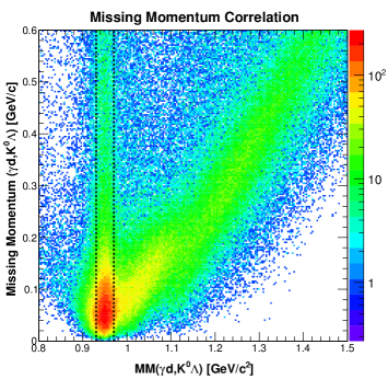
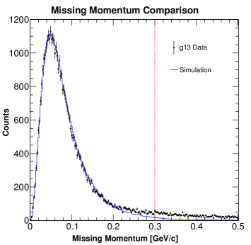
Applying a cut of MeV about the expected missing mass peak, , at the spectator proton results in Fig. 10. The agreement between simulation and data confirmed that the weighting of Fermi momentum in event generation appropriately describes the process in quasi-free events.
III.7 Systematic Uncertainties
Systematic uncertainties were determined for each portion of the experiment. This includes uncertainties in the target and detector geometries, and effects of event selection and cuts. Most components contributing to the uncertainties were compiled per kinematic bin. The largest uncertainties were associated with forward angles, where a blind spot exists from the detector geometry, and at backward angles, where statistics and detector efficiencies were poor. The average point-to-point uncertainties can be seen in Tables 1 and 2. These were separated into broad categories to give some sense of the source of uncertainty.
The systematic uncertainties underwent extensive internal review, and were examined for different choices for analysis cuts and different methods of background subtraction for the yield extraction. Details are given in Ref. Compton et al. (2014) and Compton et al. (2016). In addition, one of the largest uncertainties is due to the luminosity. This was studied extensively in Ref. Chen et al. (2009) for the g10 experiment and similar studies were repeated for the g13 experiment Compton et al. (2016). In general, these systematic uncertainties are typical when compared with other CLAS experiments McCracken et al. (2010); Bradford et al. (2006); McNabb et al. (2004).
| Investigated Cut | Systematic Uncertainty |
|---|---|
| Luminosity | 5.0% |
| Acceptance | 1.6% |
| Yield Extraction | 6.3% |
| Detector | 5.0% |
| Branching Ratios | 1.0% |
| Total | 10% |
| Investigated Cut | Systematic Uncertainty |
|---|---|
| Luminosity | 2.6-7.0% |
| Acceptance | 1.9-2.1% |
| Yield Extraction | 4.5-11.4% |
| Detector | 3.2% |
| Branching Ratios | 1.0% |
| Total | 7% - 14% |
IV Experimental Results
IV.1 Model of the Differential Cross Section
Several models, such as e.g. KAON-MAID Mart et al. (2000), have been developed for the kaon photoproduction channels. However, while most model calculations for photoproduction off the proton show little variation, due to the availability of good quality data, the predictions from KAON-MAID are largely unconstrained. The combination of the and vertices make this channel particularly hard to predict. The inclusion and exclusion of -channel kaon exchange in calculations from KAON-MAID changes the cross section output by large factors (variations up to a factor of ten as shown in Ref. Mart et al. (2000)). The present data should give enough constraints to tie down several coupling strengths that would not only improve other predictions, but possibly even allow classification of specific resonances based on extracted helicity couplings.
IV.2 Differential Cross Section
The luminosity,
| (5) |
where is the beam energy, is the atomic weight of the target, is the photon flux, is the density of the target, is the length of the target, and is Avogadro’s number, is measured as a function of beam energy in each experiment. The differential cross section for the reaction can then be written as:
| (6) |
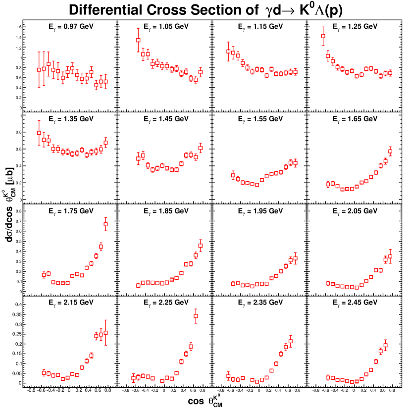
where is the bin width of , is the corrected yield, is the CLAS acceptance, and is the branching fraction or inverse branching ratios of the decay channels for the neutral hadrons (, , and ). Using the g13 data set, Fig. 11 shows the differential cross section of the reaction with respect to for 100 MeV photon energy bins between 0.9 GeV to 2.5 GeV.
Preliminary fits using PWA from the Bonn-Gatchina group were applied to the measured data Anisovich et al. (2012). The -channel diagrams, where resonances form, contain two main variables. The first unknown is that of the resonance decay, . This can be restricted by utilizing previous fit results from proton targets. The second and more interesting unknown is that of . Not only is different from that of , due to the photocouplings, but not all resonances will have a strong decay to the channels. To best describe the underlying processes, this PWA employed a multi-channel fit that incorporated observables from , , , , and . As a result of the preliminary fit, two main solutions were found to describe the data. Both solutions seem to describe and reasonably well, as shown below.
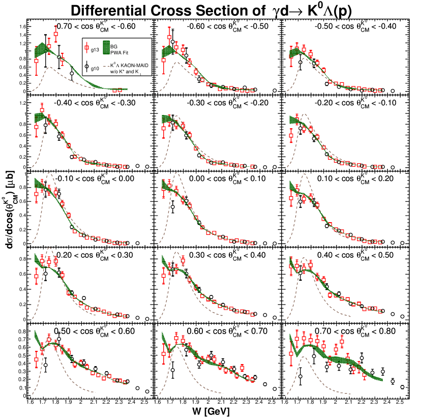
In Fig. 12, the cross section is shown as a function of center-of-mass energy for various bins including both the g10 and g13 data sets. Close agreement is seen between the two experiments, with some discrepancies in the forward bin: 0.7 0.8. Although the exact cause of the small difference in this forward bin is unknown, it is assumed that this demonstrates the uncertainty of modeling the detector and field map in this kinematic regime (two of the main differences between these experiments were the magnitude and directionality of the magnetic field). The KAON-MAID model is also shown, assuming no contributions from the and . These parameters were chosen for the model as this provided the best agreement with data. From this it is seen that these data will be essential to better constrain -channel contributions. The complementary nature of compared to , where one has a neutral exchange in the -channel and the other a charged exchange, can help differentiate between contributions from various -channel exchanges (and the interference between -channel and -channel diagrams).
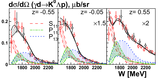
The cross sections of the data are in good agreement with the PWA fits done by the Bonn-Gatchina group Anisovich et al. (2012) as shown in Figs. 12 and 13. In the latter, the shaded regions show the range of contribution from different -channel partial waves (, and denoted in the legend of the figure) that contribute to the total strength (shown by the solid lines). Further work on measurements of photoproduction observables off the deuteron will help differentiate between the two Bonn-Gatchina solutions shown here. Such work is in progress and will be presented in a separate publication.
IV.3 Total Cross Section
The total cross section can be found by integrating over all of the differential cross section. This has two sources of uncertainty: that of the fit to the data points, and that associated with the absence of data at extreme angles.
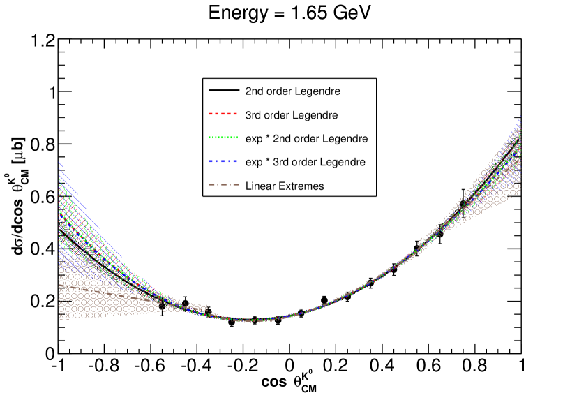
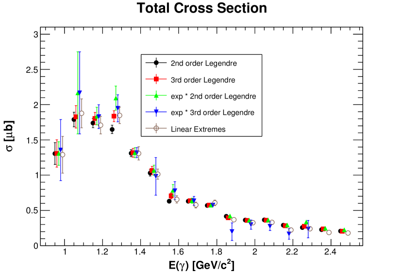
Despite the fact that an individual fit function may fit the data within the measured angular region quite well, it may not be fully representative of the overall uncertainty. To obtain an estimate on the uncertainty attributed with extrapolations to extreme regions, many functions were tried. These functions included:
-
•
A second order Legendre polynomial
-
•
A third order Legendre polynomial
-
•
A second order Legendre polynomial multiplied by an exponential
-
•
A third order Legendre polynomial multiplied by an exponential
-
•
A third order Legendre polynomial with linear extrapolations
These functions can fit the data well and be assumed to span a variation of realistic behaviors near the forward and backward angles. The uncertainty of the integration incorporated the covariance matrix given by the fit. The larger the error bands in the range of from to 1, the larger the uncertainty in the integration. Fig. 14 demonstrates several fits to the data with a 1 error band. The integrated cross sections for each fit can be seen in Fig. 15. The quoted total cross section uses the third order Legendre polynomial. The base fit is shown in Fig. 16. The inner error bars are the uncertainty estimates from the third order Legendre polynomial integration. The outer error bars represent the computed standard deviation (between third order polynomial and all other fits) added in quadrature with the inner error bars.
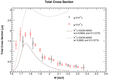
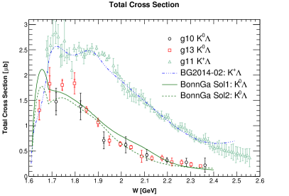
Previous analyses of Anisovich et al. (2012) have shown that there is at least one -channel resonance necessary to describe the data that was not needed for PWA of the pion data. Therefore, the channel should be able to confirm these found states. For example, Fig. 16 clearly shows a “bump” in the channel near 1900 MeV often attributed to . This enhancement is not seen in , albeit with fewer data points available. This suggests that this effect is due to missing interference terms. One interpretation is to view these missing terms as contributing to the excess cross section through the interference of a resonant state, the and -channel background processes. This is assumed since has a suppression of -channel terms Li et al. (1992), described by kaon exchange, which should make this reaction ideal for identifying resonances. This implies that partial wave analyses combined with the nature of production will be able to provide constraints for models describing nucleon resonances that couple strongly to the decay channels.
V Conclusions
In summary, the differential and total cross sections of have been presented from two different CLAS experiments, which are in good agreement. Due to the fact that previous data on this channel are scarce, the majority of presented kinematics are the first of their kind. These data have allowed a preliminary PWA fit to be completed, which produced two independent solutions to describe the intermediate processes. The PWA are being extended to fit both the present results and the previous results and other available data, with the goal of investigating whether existing -channel resonances can provide a reasonable description of these data, and perhaps to further constrain the pole properties of these ’s.
These data contain unique information that can be extracted to help with resonance classification and determination of helicity amplitudes, for example, in the contributions of the resonance in strangeness photoproduction. Clearly more investigation is needed to correctly describe the nucleon excitation spectrum. It is expected that the continued study of observables in this channel will be able to identify the best PWA solutions that can fit the data. The identification of the correct fit will improve our current understanding of the -channel contributions to cross sections.
Acknowledgements.
The authors gratefully acknowledge the work of Jefferson Lab staff in the Accelerator and Physics Divisions. This work was supported by: the United Kingdom’s Science and Technology Facilities Council (STFC); the Chilean Comisiòn Nacional de Investigaciòn Cientìfica y Tecnoĺògica (CONICYT); the Italian Istituto Nazionale di Fisica Nucleare; the French Centre National de la Recherche Scientifique; the French Commissariat à l’Energie Atomique; the U.S. National Science Foundation; and the National Research Foundation of Korea. Jefferson Science Associates, LLC, operates the Thomas Jefferson National Accelerator Facility for the the U.S. Department of Energy under Contract No. DE-AC05-06OR23177.Appendix A Table of Cross Sections
| (Stat.) | (Syst.) | |||
|---|---|---|---|---|
| (GeV) | () | () | () | |
| 1.10 | -0.65 | 1.00013 | 0.39197 | 0.10001 |
| 1.10 | -0.55 | 1.22589 | 0.27443 | 0.12259 |
| 1.10 | -0.45 | 0.71969 | 0.18661 | 0.07197 |
| 1.10 | -0.35 | 0.78350 | 0.14200 | 0.07835 |
| 1.10 | -0.25 | 0.82721 | 0.12747 | 0.08272 |
| 1.10 | -0.15 | 0.72508 | 0.10020 | 0.07251 |
| 1.10 | -0.05 | 0.77049 | 0.09670 | 0.07705 |
| 1.10 | 0.05 | 0.52375 | 0.08326 | 0.05238 |
| 1.10 | 0.15 | 0.59885 | 0.07771 | 0.05989 |
| 1.10 | 0.25 | 0.60626 | 0.08459 | 0.06063 |
| 1.10 | 0.35 | 0.66305 | 0.07958 | 0.06631 |
| 1.10 | 0.45 | 0.61605 | 0.09009 | 0.06161 |
| 1.10 | 0.55 | 0.37751 | 0.08750 | 0.03775 |
| 1.10 | 0.65 | 0.31476 | 0.10235 | 0.03148 |
| 1.10 | 0.75 | 0.23623 | 0.10792 | 0.02362 |
| 1.30 | -0.65 | 0.84988 | 0.28049 | 0.08499 |
| 1.30 | -0.55 | 0.88767 | 0.17588 | 0.08877 |
| 1.30 | -0.45 | 0.69275 | 0.09751 | 0.06927 |
| 1.30 | -0.35 | 0.57456 | 0.06604 | 0.05746 |
| 1.30 | -0.25 | 0.59504 | 0.05872 | 0.05950 |
| 1.30 | -0.15 | 0.53502 | 0.05056 | 0.05350 |
| 1.30 | -0.05 | 0.71023 | 0.04659 | 0.07102 |
| 1.30 | 0.05 | 0.60923 | 0.04677 | 0.06092 |
| 1.30 | 0.15 | 0.58598 | 0.04683 | 0.05860 |
| 1.30 | 0.25 | 0.62218 | 0.05072 | 0.06222 |
| 1.30 | 0.35 | 0.60768 | 0.04693 | 0.06077 |
| 1.30 | 0.55 | 0.70114 | 0.06825 | 0.07011 |
| 1.30 | 0.65 | 0.56572 | 0.07038 | 0.05657 |
| 1.30 | 0.75 | 0.48735 | 0.09389 | 0.04874 |
| 1.50 | -0.65 | 0.44312 | 0.16679 | 0.04431 |
| 1.50 | -0.55 | 0.30142 | 0.08267 | 0.03014 |
| 1.50 | -0.45 | 0.18577 | 0.04228 | 0.01858 |
| 1.50 | -0.35 | 0.19701 | 0.03086 | 0.01970 |
| 1.50 | -0.25 | 0.22659 | 0.02968 | 0.02266 |
| 1.50 | -0.15 | 0.24699 | 0.02800 | 0.02470 |
| 1.50 | -0.05 | 0.23696 | 0.02521 | 0.02370 |
| 1.50 | 0.05 | 0.29974 | 0.02627 | 0.02997 |
| 1.50 | 0.15 | 0.25251 | 0.02437 | 0.02525 |
| 1.50 | 0.25 | 0.35535 | 0.02824 | 0.03554 |
| 1.50 | 0.35 | 0.39293 | 0.03049 | 0.03929 |
| 1.50 | 0.45 | 0.43659 | 0.03435 | 0.04366 |
| 1.50 | 0.55 | 0.45310 | 0.04106 | 0.04531 |
| 1.50 | 0.65 | 0.38425 | 0.04451 | 0.03843 |
| 1.50 | 0.75 | 0.35311 | 0.05939 | 0.03531 |
| 1.70 | -0.55 | 0.15057 | 0.05422 | 0.01506 |
| 1.70 | -0.45 | 0.11339 | 0.02715 | 0.01134 |
| 1.70 | -0.35 | 0.14933 | 0.02108 | 0.01493 |
| 1.70 | -0.25 | 0.09314 | 0.01801 | 0.00931 |
| 1.70 | -0.15 | 0.10314 | 0.01543 | 0.01031 |
| 1.70 | -0.05 | 0.12015 | 0.01516 | 0.01202 |
| 1.70 | 0.15 | 0.18413 | 0.01695 | 0.01841 |
| 1.70 | 0.25 | 0.28597 | 0.02109 | 0.02860 |
| 1.70 | 0.35 | 0.29966 | 0.02143 | 0.02997 |
| 1.70 | 0.45 | 0.34241 | 0.02653 | 0.03424 |
| 1.70 | 0.55 | 0.40805 | 0.03285 | 0.04081 |
| 1.70 | 0.65 | 0.49763 | 0.04392 | 0.04976 |
| 1.70 | 0.75 | 0.36749 | 0.05521 | 0.03675 |
| 1.90 | -0.55 | 0.11043 | 0.03719 | 0.01104 |
| 1.90 | -0.45 | 0.05705 | 0.01839 | 0.00571 |
| 1.90 | -0.35 | 0.10543 | 0.01779 | 0.01054 |
| 1.90 | -0.25 | 0.09800 | 0.01350 | 0.00980 |
| 1.90 | -0.15 | 0.05759 | 0.01111 | 0.00576 |
| 1.90 | -0.05 | 0.05927 | 0.01208 | 0.00593 |
| 1.90 | 0.05 | 0.09919 | 0.01287 | 0.00992 |
| 1.90 | 0.15 | 0.12653 | 0.01322 | 0.01265 |
| 1.90 | 0.25 | 0.14384 | 0.01510 | 0.01438 |
| 1.90 | 0.35 | 0.19756 | 0.01787 | 0.01976 |
| 1.90 | 0.45 | 0.21230 | 0.01875 | 0.02123 |
| 1.90 | 0.55 | 0.33042 | 0.02857 | 0.03304 |
| 1.90 | 0.65 | 0.41433 | 0.03976 | 0.04143 |
| 1.90 | 0.75 | 0.32115 | 0.05167 | 0.03211 |
| 2.10 | -0.55 | 0.05985 | 0.03258 | 0.00598 |
| 2.10 | -0.45 | 0.02499 | 0.01678 | 0.00250 |
| 2.10 | -0.35 | 0.04487 | 0.01100 | 0.00449 |
| 2.10 | -0.25 | 0.04053 | 0.00926 | 0.00405 |
| 2.10 | -0.15 | 0.03574 | 0.00842 | 0.00357 |
| 2.10 | -0.05 | 0.04052 | 0.00825 | 0.00405 |
| 2.10 | 0.05 | 0.02846 | 0.00848 | 0.00285 |
| 2.10 | 0.15 | 0.06472 | 0.01016 | 0.00647 |
| 2.10 | 0.35 | 0.12534 | 0.01356 | 0.01253 |
| 2.10 | 0.45 | 0.17897 | 0.01659 | 0.01790 |
| 2.10 | 0.55 | 0.27612 | 0.02319 | 0.02761 |
| 2.10 | 0.65 | 0.32914 | 0.03134 | 0.03291 |
| 2.10 | 0.75 | 0.46576 | 0.05962 | 0.04658 |
| 2.30 | -0.55 | 0.09393 | 0.02631 | 0.00939 |
| 2.30 | -0.45 | 0.03974 | 0.01434 | 0.00397 |
| 2.30 | -0.35 | 0.01601 | 0.00850 | 0.00160 |
| 2.30 | -0.25 | 0.03098 | 0.00773 | 0.00310 |
| 2.30 | -0.15 | 0.01400 | 0.00632 | 0.00140 |
| 2.30 | -0.05 | 0.01652 | 0.00612 | 0.00165 |
| 2.30 | 0.05 | 0.02725 | 0.00635 | 0.00272 |
| 2.30 | 0.15 | 0.03218 | 0.00675 | 0.00322 |
| 2.30 | 0.25 | 0.06879 | 0.00908 | 0.00688 |
| 2.30 | 0.35 | 0.10418 | 0.01186 | 0.01042 |
| 2.30 | 0.45 | 0.14920 | 0.01497 | 0.01492 |
| 2.30 | 0.55 | 0.18561 | 0.01928 | 0.01856 |
| 2.30 | 0.65 | 0.23703 | 0.02506 | 0.02370 |
| 2.30 | 0.75 | 0.28270 | 0.04309 | 0.02827 |
| 2.50 | -0.55 | 0.04511 | 0.02009 | 0.00451 |
| 2.50 | -0.45 | 0.03033 | 0.00999 | 0.00303 |
| 2.50 | -0.35 | 0.01442 | 0.00675 | 0.00144 |
| 2.50 | -0.25 | 0.01399 | 0.00549 | 0.00140 |
| 2.50 | -0.15 | 0.01566 | 0.00544 | 0.00157 |
| 2.50 | -0.05 | 0.01149 | 0.00374 | 0.00115 |
| 2.50 | 0.05 | 0.00996 | 0.00572 | 0.00100 |
| 2.50 | 0.15 | 0.02832 | 0.00729 | 0.00283 |
| 2.50 | 0.25 | 0.04826 | 0.00821 | 0.00483 |
| 2.50 | 0.35 | 0.07632 | 0.01049 | 0.00763 |
| 2.50 | 0.45 | 0.11663 | 0.01322 | 0.01166 |
| 2.50 | 0.55 | 0.17365 | 0.01968 | 0.01736 |
| 2.50 | 0.65 | 0.22403 | 0.02580 | 0.02240 |
| 2.50 | 0.75 | 0.29691 | 0.04540 | 0.02969 |
| 2.70 | -0.45 | 0.01367 | 0.01099 | 0.00137 |
| 2.70 | -0.35 | 0.03146 | 0.00891 | 0.00315 |
| 2.70 | -0.25 | 0.00871 | 0.00492 | 0.00087 |
| 2.70 | -0.15 | 0.00528 | 0.00365 | 0.00053 |
| 2.70 | -0.05 | 0.00695 | 0.00407 | 0.00070 |
| 2.70 | 0.05 | 0.00555 | 0.00455 | 0.00056 |
| 2.70 | 0.15 | 0.01532 | 0.00523 | 0.00153 |
| 2.70 | 0.25 | 0.02582 | 0.00634 | 0.00258 |
| 2.70 | 0.35 | 0.06135 | 0.00945 | 0.00614 |
| 2.70 | 0.45 | 0.07578 | 0.01138 | 0.00758 |
| 2.70 | 0.55 | 0.09083 | 0.01279 | 0.00908 |
| 2.70 | 0.65 | 0.13890 | 0.01846 | 0.01389 |
| 2.70 | 0.75 | 0.17514 | 0.03573 | 0.01751 |
| 2.90 | -0.55 | 0.02295 | 0.01465 | 0.00230 |
| 2.90 | -0.35 | 0.01680 | 0.00546 | 0.00168 |
| 2.90 | -0.25 | 0.00971 | 0.00376 | 0.00097 |
| 2.90 | 0.05 | 0.00359 | 0.00222 | 0.00036 |
| 2.90 | 0.15 | 0.01019 | 0.00284 | 0.00102 |
| 2.90 | 0.25 | 0.01012 | 0.00403 | 0.00101 |
| 2.90 | 0.35 | 0.02945 | 0.00543 | 0.00294 |
| 2.90 | 0.45 | 0.04284 | 0.00702 | 0.00428 |
| 2.90 | 0.55 | 0.04900 | 0.00873 | 0.00490 |
| 2.90 | 0.65 | 0.08143 | 0.01379 | 0.00814 |
| 2.90 | 0.75 | 0.10337 | 0.02153 | 0.01034 |
| (Stat.) | (Syst.) | |||
|---|---|---|---|---|
| (GeV) | () | () | () | |
| 0.97 | -0.65 | 0.75255 | 0.35076 | 0.06867 |
| 0.97 | -0.55 | 0.77160 | 0.33467 | 0.07040 |
| 0.97 | -0.45 | 0.86497 | 0.24008 | 0.07892 |
| 0.97 | -0.35 | 0.74992 | 0.17343 | 0.06843 |
| 0.97 | -0.25 | 0.72369 | 0.17066 | 0.06603 |
| 0.97 | -0.15 | 0.59180 | 0.11788 | 0.05400 |
| 0.97 | -0.05 | 0.70802 | 0.11000 | 0.06460 |
| 0.97 | 0.05 | 0.78103 | 0.11056 | 0.07126 |
| 0.97 | 0.15 | 0.64846 | 0.10411 | 0.05917 |
| 0.97 | 0.25 | 0.57306 | 0.09379 | 0.05229 |
| 0.97 | 0.35 | 0.57949 | 0.09745 | 0.05287 |
| 0.97 | 0.45 | 0.70460 | 0.10752 | 0.06429 |
| 0.97 | 0.55 | 0.44682 | 0.09608 | 0.04077 |
| 0.97 | 0.65 | 0.51625 | 0.12026 | 0.04710 |
| 0.97 | 0.75 | 0.51830 | 0.14436 | 0.04729 |
| 1.05 | -0.55 | 1.33875 | 0.23334 | 0.10225 |
| 1.05 | -0.45 | 1.05646 | 0.12457 | 0.08069 |
| 1.05 | -0.35 | 1.05996 | 0.10028 | 0.08096 |
| 1.05 | -0.25 | 0.86644 | 0.08602 | 0.06618 |
| 1.05 | -0.15 | 0.88866 | 0.07516 | 0.06788 |
| 1.05 | -0.05 | 0.82451 | 0.06602 | 0.06298 |
| 1.05 | 0.05 | 0.82510 | 0.06255 | 0.06302 |
| 1.05 | 0.15 | 0.75963 | 0.05883 | 0.05802 |
| 1.05 | 0.25 | 0.77430 | 0.05987 | 0.05914 |
| 1.05 | 0.35 | 0.67270 | 0.05781 | 0.05138 |
| 1.05 | 0.45 | 0.71069 | 0.06013 | 0.05428 |
| 1.05 | 0.55 | 0.57955 | 0.05932 | 0.04427 |
| 1.05 | 0.65 | 0.55457 | 0.07076 | 0.04236 |
| 1.05 | 0.75 | 0.70325 | 0.09656 | 0.05372 |
| 1.15 | -0.65 | 1.11443 | 0.18921 | 0.07850 |
| 1.15 | -0.55 | 1.08909 | 0.12420 | 0.07672 |
| 1.15 | -0.45 | 1.03075 | 0.08920 | 0.07261 |
| 1.15 | -0.35 | 0.88525 | 0.06737 | 0.06236 |
| 1.15 | -0.25 | 0.79475 | 0.05571 | 0.05598 |
| 1.15 | -0.15 | 0.71598 | 0.04944 | 0.05043 |
| 1.15 | -0.05 | 0.75928 | 0.04681 | 0.05348 |
| 1.15 | 0.05 | 0.74950 | 0.04504 | 0.05279 |
| 1.15 | 0.15 | 0.63681 | 0.03979 | 0.04486 |
| 1.15 | 0.25 | 0.76139 | 0.04296 | 0.05363 |
| 1.15 | 0.35 | 0.66951 | 0.04196 | 0.04716 |
| 1.15 | 0.45 | 0.67394 | 0.04344 | 0.04747 |
| 1.15 | 0.55 | 0.69452 | 0.04952 | 0.04892 |
| 1.15 | 0.65 | 0.71138 | 0.05281 | 0.05011 |
| 1.15 | 0.75 | 0.70978 | 0.06620 | 0.05000 |
| 1.25 | -0.65 | 1.41869 | 0.18279 | 0.09557 |
| 1.25 | -0.55 | 1.02626 | 0.10700 | 0.06913 |
| 1.25 | -0.45 | 0.92005 | 0.07879 | 0.06198 |
| 1.25 | -0.35 | 0.80255 | 0.05824 | 0.05406 |
| 1.25 | -0.25 | 0.76759 | 0.05021 | 0.05171 |
| 1.25 | -0.15 | 0.70174 | 0.04323 | 0.04727 |
| 1.25 | -0.05 | 0.72802 | 0.04088 | 0.04904 |
| 1.25 | 0.05 | 0.62247 | 0.03618 | 0.04193 |
| 1.25 | 0.15 | 0.65450 | 0.03824 | 0.04409 |
| 1.25 | 0.25 | 0.77066 | 0.03968 | 0.05191 |
| 1.25 | 0.35 | 0.77760 | 0.03932 | 0.05238 |
| 1.25 | 0.45 | 0.72072 | 0.04070 | 0.04855 |
| 1.25 | 0.55 | 0.62717 | 0.04325 | 0.04225 |
| 1.25 | 0.65 | 0.67817 | 0.04858 | 0.04568 |
| 1.25 | 0.75 | 0.68653 | 0.06194 | 0.04625 |
| 1.35 | -0.65 | 0.79066 | 0.14608 | 0.05183 |
| 1.35 | -0.55 | 0.70911 | 0.08701 | 0.04649 |
| 1.35 | -0.45 | 0.70095 | 0.06063 | 0.04596 |
| 1.35 | -0.35 | 0.60235 | 0.04678 | 0.03949 |
| 1.35 | -0.25 | 0.59899 | 0.04013 | 0.03927 |
| 1.35 | -0.15 | 0.56432 | 0.03514 | 0.03700 |
| 1.35 | -0.05 | 0.56618 | 0.03263 | 0.03712 |
| 1.35 | 0.05 | 0.53946 | 0.03094 | 0.03537 |
| 1.35 | 0.15 | 0.54716 | 0.03028 | 0.03587 |
| 1.35 | 0.25 | 0.58681 | 0.03221 | 0.03847 |
| 1.35 | 0.35 | 0.52749 | 0.03141 | 0.03458 |
| 1.35 | 0.45 | 0.56359 | 0.03440 | 0.03695 |
| 1.35 | 0.55 | 0.57093 | 0.03933 | 0.03743 |
| 1.35 | 0.65 | 0.59598 | 0.04497 | 0.03907 |
| 1.35 | 0.75 | 0.67498 | 0.06028 | 0.04425 |
| 1.45 | -0.55 | 0.48669 | 0.07164 | 0.03173 |
| 1.45 | -0.45 | 0.52218 | 0.05000 | 0.03460 |
| 1.45 | -0.35 | 0.40599 | 0.03659 | 0.02647 |
| 1.45 | -0.25 | 0.35432 | 0.02933 | 0.02310 |
| 1.45 | -0.15 | 0.37073 | 0.02726 | 0.02417 |
| 1.45 | -0.05 | 0.40146 | 0.02634 | 0.02617 |
| 1.45 | 0.05 | 0.37243 | 0.02412 | 0.02428 |
| 1.45 | 0.15 | 0.35336 | 0.02461 | 0.02304 |
| 1.45 | 0.25 | 0.35558 | 0.02463 | 0.02318 |
| 1.45 | 0.35 | 0.42516 | 0.02640 | 0.02772 |
| 1.45 | 0.45 | 0.52429 | 0.03086 | 0.03418 |
| 1.45 | 0.55 | 0.53086 | 0.03503 | 0.03460 |
| 1.45 | 0.65 | 0.50279 | 0.03859 | 0.03277 |
| 1.45 | 0.75 | 0.61126 | 0.05597 | 0.03984 |
| 1.55 | -0.55 | 0.28879 | 0.05107 | 0.01964 |
| 1.55 | -0.45 | 0.24327 | 0.03220 | 0.01633 |
| 1.55 | -0.35 | 0.20305 | 0.02309 | 0.01362 |
| 1.55 | -0.25 | 0.19669 | 0.01976 | 0.01320 |
| 1.55 | -0.15 | 0.18372 | 0.01760 | 0.01233 |
| 1.55 | -0.05 | 0.17685 | 0.01688 | 0.01193 |
| 1.55 | 0.05 | 0.23188 | 0.01803 | 0.01559 |
| 1.55 | 0.15 | 0.27718 | 0.01856 | 0.01865 |
| 1.55 | 0.25 | 0.30317 | 0.01888 | 0.02034 |
| 1.55 | 0.35 | 0.31162 | 0.02078 | 0.02092 |
| 1.55 | 0.45 | 0.32393 | 0.02346 | 0.02173 |
| 1.55 | 0.55 | 0.38605 | 0.02834 | 0.02589 |
| 1.55 | 0.65 | 0.43859 | 0.03520 | 0.02941 |
| 1.55 | 0.75 | 0.43297 | 0.04882 | 0.02904 |
| 1.65 | -0.55 | 0.18039 | 0.03551 | 0.01216 |
| 1.65 | -0.45 | 0.19119 | 0.02561 | 0.01243 |
| 1.65 | -0.35 | 0.15919 | 0.01849 | 0.01034 |
| 1.65 | -0.25 | 0.12044 | 0.01560 | 0.00784 |
| 1.65 | -0.15 | 0.12797 | 0.01427 | 0.00831 |
| 1.65 | -0.05 | 0.12656 | 0.01391 | 0.00827 |
| 1.65 | 0.05 | 0.15465 | 0.01498 | 0.01005 |
| 1.65 | 0.15 | 0.20314 | 0.01597 | 0.01322 |
| 1.65 | 0.25 | 0.21709 | 0.01689 | 0.01409 |
| 1.65 | 0.35 | 0.26907 | 0.01870 | 0.01750 |
| 1.65 | 0.45 | 0.32082 | 0.02180 | 0.02082 |
| 1.65 | 0.55 | 0.40120 | 0.02820 | 0.02604 |
| 1.65 | 0.65 | 0.45581 | 0.03610 | 0.02958 |
| 1.65 | 0.75 | 0.57200 | 0.05412 | 0.03713 |
| 1.75 | -0.55 | 0.16534 | 0.03194 | 0.01111 |
| 1.75 | -0.45 | 0.17897 | 0.02230 | 0.01203 |
| 1.75 | -0.35 | 0.09317 | 0.01530 | 0.00629 |
| 1.75 | -0.25 | 0.08305 | 0.01289 | 0.00559 |
| 1.75 | -0.15 | 0.08291 | 0.01206 | 0.00561 |
| 1.75 | -0.05 | 0.08655 | 0.01213 | 0.00585 |
| 1.75 | 0.05 | 0.15390 | 0.01382 | 0.01036 |
| 1.75 | 0.15 | 0.17531 | 0.01541 | 0.01184 |
| 1.75 | 0.25 | 0.16149 | 0.01470 | 0.01089 |
| 1.75 | 0.35 | 0.23698 | 0.01728 | 0.01593 |
| 1.75 | 0.45 | 0.27890 | 0.02071 | 0.01874 |
| 1.75 | 0.55 | 0.35337 | 0.02587 | 0.02375 |
| 1.75 | 0.65 | 0.44786 | 0.03696 | 0.03009 |
| 1.75 | 0.75 | 0.66910 | 0.06598 | 0.04495 |
| 1.85 | -0.55 | 0.06010 | 0.02025 | 0.00409 |
| 1.85 | -0.45 | 0.08868 | 0.01599 | 0.00592 |
| 1.85 | -0.35 | 0.09077 | 0.01371 | 0.00609 |
| 1.85 | -0.25 | 0.08972 | 0.01144 | 0.00600 |
| 1.85 | -0.15 | 0.08442 | 0.01091 | 0.00564 |
| 1.85 | -0.05 | 0.08094 | 0.01062 | 0.00550 |
| 1.85 | 0.05 | 0.09120 | 0.01044 | 0.00611 |
| 1.85 | 0.15 | 0.11921 | 0.01208 | 0.00797 |
| 1.85 | 0.25 | 0.13622 | 0.01293 | 0.00913 |
| 1.85 | 0.35 | 0.18348 | 0.01470 | 0.01226 |
| 1.85 | 0.45 | 0.27127 | 0.01847 | 0.01812 |
| 1.85 | 0.55 | 0.27746 | 0.02227 | 0.01853 |
| 1.85 | 0.65 | 0.36097 | 0.03286 | 0.02411 |
| 1.85 | 0.75 | 0.45618 | 0.05999 | 0.03046 |
| 1.95 | -0.55 | 0.07889 | 0.02144 | 0.00520 |
| 1.95 | -0.45 | 0.08362 | 0.01455 | 0.00557 |
| 1.95 | -0.35 | 0.06207 | 0.01126 | 0.00407 |
| 1.95 | -0.25 | 0.06722 | 0.01060 | 0.00441 |
| 1.95 | -0.15 | 0.05209 | 0.00908 | 0.00342 |
| 1.95 | -0.05 | 0.07212 | 0.00919 | 0.00475 |
| 1.95 | 0.05 | 0.07863 | 0.00974 | 0.00516 |
| 1.95 | 0.15 | 0.07853 | 0.01053 | 0.00527 |
| 1.95 | 0.25 | 0.13154 | 0.01223 | 0.00863 |
| 1.95 | 0.35 | 0.15496 | 0.01353 | 0.01018 |
| 1.95 | 0.45 | 0.20197 | 0.01687 | 0.01325 |
| 1.95 | 0.55 | 0.25252 | 0.02099 | 0.01654 |
| 1.95 | 0.65 | 0.31196 | 0.03198 | 0.02044 |
| 1.95 | 0.75 | 0.33056 | 0.05756 | 0.02165 |
| 2.05 | -0.55 | 0.08179 | 0.01988 | 0.00541 |
| 2.05 | -0.45 | 0.07376 | 0.01232 | 0.00484 |
| 2.05 | -0.35 | 0.05625 | 0.01004 | 0.00369 |
| 2.05 | -0.25 | 0.05190 | 0.00905 | 0.00342 |
| 2.05 | -0.15 | 0.04399 | 0.00838 | 0.00289 |
| 2.05 | -0.05 | 0.04490 | 0.00883 | 0.00295 |
| 2.05 | 0.05 | 0.04106 | 0.00909 | 0.00274 |
| 2.05 | 0.15 | 0.06679 | 0.00953 | 0.00450 |
| 2.05 | 0.25 | 0.10552 | 0.01140 | 0.00696 |
| 2.05 | 0.35 | 0.14621 | 0.01330 | 0.00961 |
| 2.05 | 0.45 | 0.21218 | 0.01649 | 0.01393 |
| 2.05 | 0.55 | 0.21077 | 0.02012 | 0.01383 |
| 2.05 | 0.65 | 0.31704 | 0.03580 | 0.02079 |
| 2.05 | 0.75 | 0.35042 | 0.06888 | 0.02320 |
| 2.15 | -0.55 | 0.05246 | 0.01674 | 0.00358 |
| 2.15 | -0.45 | 0.04878 | 0.01137 | 0.00327 |
| 2.15 | -0.35 | 0.03869 | 0.00911 | 0.00263 |
| 2.15 | -0.25 | 0.04184 | 0.00779 | 0.00281 |
| 2.15 | -0.15 | 0.02167 | 0.00702 | 0.00147 |
| 2.15 | -0.05 | 0.02822 | 0.00731 | 0.00190 |
| 2.15 | 0.05 | 0.04655 | 0.00874 | 0.00313 |
| 2.15 | 0.15 | 0.04077 | 0.00771 | 0.00276 |
| 2.15 | 0.25 | 0.07932 | 0.00974 | 0.00546 |
| 2.15 | 0.35 | 0.11273 | 0.01140 | 0.00756 |
| 2.15 | 0.45 | 0.14085 | 0.01349 | 0.00944 |
| 2.15 | 0.55 | 0.24018 | 0.02003 | 0.01609 |
| 2.15 | 0.65 | 0.24749 | 0.02982 | 0.01658 |
| 2.15 | 0.75 | 0.25732 | 0.06418 | 0.01761 |
| 2.25 | -0.65 | 0.02567 | 0.02226 | 0.00180 |
| 2.25 | -0.55 | 0.02952 | 0.01342 | 0.00207 |
| 2.25 | -0.45 | 0.03718 | 0.00992 | 0.00261 |
| 2.25 | -0.35 | 0.03327 | 0.00812 | 0.00232 |
| 2.25 | -0.25 | 0.02416 | 0.00730 | 0.00167 |
| 2.25 | -0.05 | 0.01092 | 0.00615 | 0.00076 |
| 2.25 | 0.05 | 0.02809 | 0.00760 | 0.00194 |
| 2.25 | 0.15 | 0.02312 | 0.00776 | 0.00160 |
| 2.25 | 0.25 | 0.05048 | 0.00915 | 0.00350 |
| 2.25 | 0.35 | 0.10989 | 0.01185 | 0.00758 |
| 2.25 | 0.45 | 0.14907 | 0.01409 | 0.01029 |
| 2.25 | 0.55 | 0.18725 | 0.01990 | 0.01292 |
| 2.25 | 0.65 | 0.34181 | 0.03665 | 0.02358 |
| 2.35 | -0.65 | 0.03675 | 0.02146 | 0.00345 |
| 2.35 | -0.55 | 0.01943 | 0.01110 | 0.00183 |
| 2.35 | -0.45 | 0.01774 | 0.00968 | 0.00116 |
| 2.35 | -0.35 | 0.02601 | 0.00736 | 0.00171 |
| 2.35 | -0.15 | 0.01446 | 0.00687 | 0.00096 |
| 2.35 | -0.05 | 0.00745 | 0.00587 | 0.00049 |
| 2.35 | 0.05 | 0.01752 | 0.00583 | 0.00115 |
| 2.35 | 0.15 | 0.02863 | 0.00707 | 0.00188 |
| 2.35 | 0.25 | 0.06421 | 0.00835 | 0.00422 |
| 2.35 | 0.35 | 0.09907 | 0.01024 | 0.00648 |
| 2.35 | 0.45 | 0.14870 | 0.01386 | 0.00973 |
| 2.35 | 0.55 | 0.18374 | 0.01835 | 0.01201 |
| 2.35 | 0.65 | 0.21345 | 0.03008 | 0.01397 |
| 2.45 | -0.55 | 0.02850 | 0.01312 | 0.01366 |
| 2.45 | -0.45 | 0.02657 | 0.00862 | 0.00176 |
| 2.45 | -0.35 | 0.01547 | 0.00692 | 0.00104 |
| 2.45 | -0.25 | 0.01802 | 0.00650 | 0.00118 |
| 2.45 | -0.15 | 0.01117 | 0.00549 | 0.00090 |
| 2.45 | -0.05 | 0.00628 | 0.00609 | 0.00042 |
| 2.45 | 0.05 | 0.00882 | 0.00631 | 0.00057 |
| 2.45 | 0.15 | 0.02063 | 0.00613 | 0.00135 |
| 2.45 | 0.25 | 0.04485 | 0.00731 | 0.00292 |
| 2.45 | 0.35 | 0.06794 | 0.00913 | 0.00442 |
| 2.45 | 0.45 | 0.11035 | 0.01167 | 0.00718 |
| 2.45 | 0.55 | 0.16248 | 0.01689 | 0.01057 |
| 2.45 | 0.65 | 0.19303 | 0.02777 | 0.01260 |
References
- Patrignani et al. (2016) C. Patrignani et al. (Particle Data Group), Chin. Phys. C40, 100001 (2016).
- Anisovich et al. (2012) A. V. Anisovich, R. Beck, E. Klempt, V. A. Nikonov, A. V. Sarantsev, and U. Thoma, The European Physical Journal A 48, 1 (2012).
- Close (1979) F. E. Close, An Introduction to Quarks and Partons (Academic Press Inc., 111 Fifth Avenue, NewYork, NewYork 10003, 1979).
- Zachariou (2017) N. Zachariou, Few-Body Systems 58, 72 (2017).
- Mart et al. (2000) T. Mart, C. Bennhold, H. Haberzettl, and L. Tiator, “KAON-MAID 2000,” (2000).
- McCracken et al. (2010) M. E. McCracken, M. Bellis, C. A. Meyer, M. Williams et al. (CLAS Collaboration), Phys. Rev. C 81, 025201 (2010).
- Bradford et al. (2006) R. Bradford, R. A. Schumacher, J. W. C. McNabb, L. Todor et al. (CLAS Collaboration), Phys. Rev. C 73, 035202 (2006).
- McNabb et al. (2004) J. W. C. McNabb, R. A. Schumacher, L. Todor et al. (CLAS Collaboration), Phys. Rev. C 69, 042201 (2004).
- Koniuk and Isgur (1980) R. Koniuk and N. Isgur, Phys. Rev. D 21, 1868 (1980).
- Capstick and Roberts (1998) S. Capstick and W. Roberts, Phys. Rev. D 58, 074011 (1998).
- Edwards et al. (2013) R. G. Edwards, N. Mathur, D. G. Richards, and S. J. Wallace (Hadron Spectrum Collaboration), Phys. Rev. D 87, 054506 (2013).
- Tran et al. (1998) M. Tran, J. Barth, C. Bennhold et al., Physics Letters B 445, 20 (1998).
- Glander et al. (2004) K. H. Glander et al., Eur. Phys. J. A19, 251 (2004).
- Sober et al. (2000) D. I. Sober et al., Nucl. Instrum. Meth. A440, 263 (2000).
- Mestayer et al. (2000) M. D. Mestayer et al., Nucl. Instrum. Meth. A449, 81 (2000).
- Mecking et al. (2003) B. A. Mecking et al., Nucl. Instrum. Meth. A503, 513 (2003).
- Taylor et al. (2001) S. Taylor, S. Ahmad, J. Distelbrink, G. S. Mutchler, E. Smith, and T. Smith, Nucl. Instrum. Meth. A462, 484 (2001).
- Sharabian et al. (2006) Y. Sharabian, M. Battaglieri, V. Burkert, R. DeVita, L. Elouadrhiri, L. Guo, D. Kashy, V. Kubarovsky, G. Mutchler, M. Ostrick, M. Ripani, P. Rossi, A. Rottura, E. Pasyuk, and D. Weygand, Nucl. Instrum. Meth. 556, 246 (2006).
- Chen et al. (2009) W. Chen, T. Mibe, D. Dutta, H. Gao, J. M. Laget, M. Mirazita, P. Rossi, S. Stepanyan, I. I. Strakovsky et al. (CLAS Collaboration), Phys. Rev. Lett. 103, 012301 (2009).
- Compton et al. (2014) N. Compton, K. Hicks, and M. Camp, Cross Sections of from g10 (2014), CLAS analysis note.
- Compton et al. (2016) N. Compton, C. E. Taylor, K. Hicks, P. Cole et al., Photoproduction on the Neutron within the Resonance Region (2016), CLAS analysis note.
- Pasyuk (2007) E. Pasyuk (CLAS Collaboration), Energy loss corrections for charged particles in CLAS (2007), CLAS-Note 2007-016.
- Nadel-Turonski et al. (2006) P. Nadel-Turonski, B. Berman, Y. Ilieva, A. Tkabladze, D. Ireland et al. (CLAS Collaboration), Kaon Production on the Deuteron Using Polarized Photons (2006), Jefferson Lab PAC30 Proposal.
- Ball and Pasyuk (2005) J. Ball and E. Pasyuk (CLAS Collaboration), Photon Flux Determination Through Sampling of “out-of-time” Hits with the Hall B Photon Tagger (2005), CLAS-Note 2005-002.
- (25) S. Stepanyan, “fsgen phase space generator,” (private communication).
- Christiansen et al. (2007) J. Christiansen, N. Desai, P. Ilten, S. Mrenna, S. Prestel, C. Rasmussen, T. Sjöstrand, and P. Skands, “Pythia,” (2007).
- Machleidt (2001) R. Machleidt, Phys. Rev. C63, 024001 (2001).
- Li et al. (1992) X. Li, L. E. Wright, and C. Bennhold, Phys. Rev. C 45, 2011 (1992).