:
\theoremsep
\jmlrvolume1
\jmlryear2017
\jmlrworkshopICML 2017 AutoML Workshop
Dealing with Integer-valued Variables in Bayesian Optimization with Gaussian Processes
Abstract
Bayesian optimization (BO) methods are useful for optimizing functions that are expensive to evaluate, lack an analytical expression and whose evaluations can be contaminated by noise. These methods rely on a probabilistic model of the objective function, typically a Gaussian process (GP), upon which an acquisition function is built. This function guides the optimization process and measures the expected utility of performing an evaluation of the objective at a new point. GPs assume continous input variables. When this is not the case, such as when some of the input variables take integer values, one has to introduce extra approximations. A common approach is to round the suggested variable value to the closest integer before doing the evaluation of the objective. We show that this can lead to problems in the optimization process and describe a more principled approach to account for input variables that are integer-valued. We illustrate in both synthetic and a real experiments the utility of our approach, which significantly improves the results of standard BO methods on problems involving integer-valued variables.
keywords:
Parameter tuning, Bayesian optimization, Gaussian processes, Integer-valued variables.1 Background on Bayesian Optimization
Bayesian optimization (BO) methods (Shahriari et al., 2016) address the problem of optimizing a real-valued function over some bounded domain . The objective function is assumed to lack an analytical expression (which prevents any gradient computation), to be very expensive to evaluate, and the evaluations are assumed to be noisy (i.e., rather than observing we observe , with some additive noise). At each iteration of the optimization process, BO methods fit a probabilistic model, typically a Gaussian process (GP) (Rasmussen and Williams, 2006), to the observations of the objective function collected so far. The uncertainty about the potential values of the objective function provided by the GP is then used to generate an acquisition function , whose value at each input location indicates the expected utility of evaluating there. The next point at which to evaluate is the one that maximizes . After collecting this observation, the process is repeated. When enough data has been collected, the GP predictive mean value for can be optimized to find the solution of the problem.
The key for BO success is that evaluating the acquisition function is very cheap compared to the evaluation of . This is so because the acquisition function only depends on the GP predictive distribution for at a candidate point . Thus, can be maximized with very little cost. BO methods hence spend a small amount of time thinking very carefully where to evaluate next the objective function with the aim of finding its optimum with the smallest number of evaluations. This is a very useful strategy when the objective function is very expensive to evaluate and it can save a lot of computational time.
Let the observed data until step of the algorithm be . The GP predictive distribution for is given by a Gaussian distribution characterized by a mean and a variance . These values are:
| (1) |
where is a vector with the objective values observed so far; is a vector with the prior covariances between and each ; is the variance of the additive Gaussian noise; is a matrix with the prior covariances among each , for ; and is the prior variance at the candidate location . These quantities are obtained from a covariance function which is pre-specified and receives as an input and at which the covariance between and is evaluated. A typical covariance function employed in BO is the Matérn function (Snoek et al., 2012).
A popular acquisition function is expected improvement (EI) (Jones et al., 1998). EI is given by the expected value of the utility function under the GP predictive distribution for , where is the best value observed so far (assuming minimization). Thus, EI measures on average how much we will improve on the current best solution by performing an evaluation at each candidate point. The EI acquisition function is , where and and are respectively the c.d.f. and p.d.f. of a standard Gaussian.
2 Dealing with Integer-valued Variables
The framework described assumes continous input variables in . This is so because in a GP the variables introduced in the covariance function are assumed to be continous. A problem may arise when some of the inputs can only take values in a closed subset of a discrete set, such as the integers. If this is the case, the GP process will ignore that constraint and will place some probability mass on invalid potential values for . These incorrect modeling assumptions about the objective may have a negative impact on the optimization process. Furthermore, the optimization of will typically provide candidate points at which to evaluate the objective that are invalid in the sense that integer-valued input variables will be assigned real values. In practice, some mechanism to transform real values into integer values must be implemented before the evaluation can take place. If this is not done with care, some problems may appear in the optimization process.
Optimization problems involving continuous and discrete variables appear in the task of optimizing the hyper-parameters of machine learning systems (Snoek et al., 2012). For example, in a deep neural network we may be interested in adjusting the learning rate, the number of layers and the number of neurons per layer, which can only take discrete values. Similarly, in a ensemble of decision trees generated by the gradient boosting algorithm (Friedman, 2001) we may try to adjust the learning rate and the maximum depth of the trees. This last hyper-parameter can only take discrete values. A last example involves a nearest neighbor classifier. In this case we may be interested in finding the optimal number of neighbors and the optimal scaling factor per dimension to be used in the computation of the distance. The number of neighbors can only take discrete values.
|
Naive |
 |
 |
|---|---|---|
|
Basic |
 |
 |
|
Proposed |
 |
 |
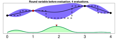
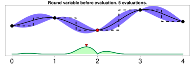
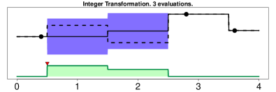
A naive approach to consider that the objective can only be evaluated at integer values in some of the inputs is to (i) optimize assuming all variables take values in the real line, and (ii) replace all the values for the integer-valued variables by the closest integer. This is the approach followed by the popular software for BO Spearmint (https://github.com/HIPS/Spearmint). However, as shown in the first row of Figure 1 this can lead to a mismatch between the points in which the acquisition takes high values, and where the actual evaluation is performed. Furthermore, it can produce situations in which the BO method always evaluates the objective at a point where it has already been evaluated (because the next and following evaluations will not change at all the acquisition function). For this reason, we discourage the use of this approach.
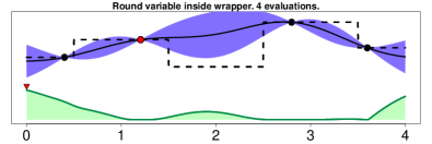
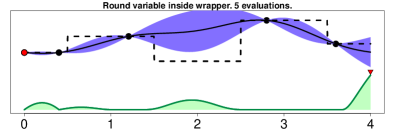
The previous problem can be solved by doing the rounding to the closest integer value inside the wrapper that evaluates the objective. This basic approach is shown in the second row of Figure 1. In this case the points at which the acquisition takes high values and the points at which the objective is evaluated coincide. Thus, the BO method will tend to evaluate at different locations, as expected. The problem is, however, that the actual objective is constant in the intervals that are rounded to the same integer value. This constant behavior is ignored by the GP, which can be sub-optimal.
3 Proposed Approach
We propose a method to alleviate the problems of the basic approach of Section 2. For this, we consider that the objective should be constant in the intervals that are rounded to the same integer. This property can be easily introduced in the GP by modifying . Covariance functions are often stationary and only depend on the distance between the input points. If the distance between two points its zero, the values of the function at both points will be the same (the correlation is equal to one). Based on this fact, we suggest to transform the input points to , obtaining an alternative covariance function :
| (2) |
where is a transformation in which all integer-valued variables of in are rounded to the closest integer. The beneficial properties of when used for BO are illustrated in the third row of Figure 1. We can see that the GP model correctly identifies that the objective function is constant inside intervals of real values that are rounded to the same integer. The uncertainty is also the same in those intervals, and this is reflected in the acquisition function. Furthermore, after performing a single measurement in each interval, the uncertainty about goes to zero. This better modeling of the objective is expected to be reflected in a better performance of the optimization process.
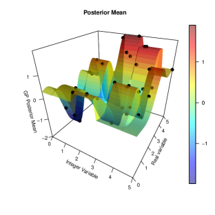
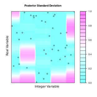
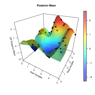
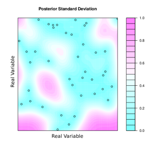
Figure 2 illustrates the modelling properties of the proposed covariance function (2). It shows the mean and standard deviation of the posterior distribution given some observations. It compares results with a standard GP that does not use the proposed transformation. In this case the data has been sampled from a GP using the covariance function in (2) with the squared exponential covariance function (Rasmussen and Williams, 2006). One dimension takes continuous vales and the other values in . Note that the posterior distribution captures the constant behavior of the function in any interval of values that are rounded to the same integer, only for the integer dimension (top). A standard GP (corresponding to the basic approach in Section 2) cannot capture this (bottom).
|
Proposed Approach |
 |
 |
|---|---|---|
|
Standard GP |
 |
 |
4 Experiments
We compare the performance of the proposed approach for BO with the basic approach described in Section 2. Each method has been implemented in the software for BO Spearmint. We use a Matérn covariance function, and estimate the GP hyper-parameters using slice sampling (Murray and Adams, 2010). The acquisition function employed is EI.
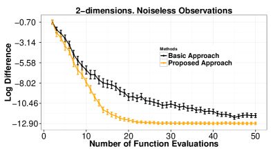
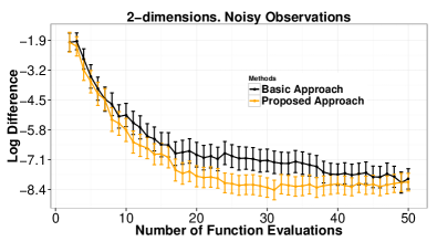
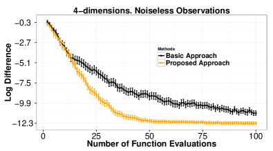
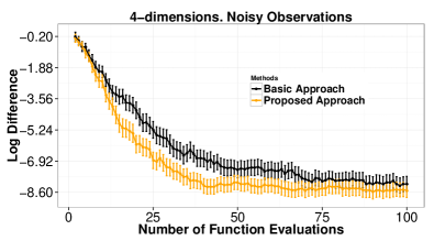
A first batch of experiments considers two synthetic objectives. The first objective depends on 2 variables. In this case the first variable takes values in the interval , and the second variable takes values in the set . The second objective depends on 4 variables. In this case the first 2 variables take values in the interval . The remaining 2 variables take values in the set and , respectively. In each case, we sample the objectives from a GP prior using (2) as the covariance function. We run each BO method (proposed and basic) for 50 and 100 iterations, in the case of each objective, and report the logarithm of the distance to the minimum value of each objective as a function of the evaluations done. We consider 100 repetitions of the experiments. We also consider these experiments when the objectives are contaminated with additive Gaussian noise with variance and , respectively. The results obtained are displayed in Figure 3. We observe that the proposed approach gives better results than the basic approach. In particular, it finds points that are closer to the optimal one with a smaller number of evaluations of the objective, both in the case of noisy and noiseless evaluations.
 |
 |
 |
 |
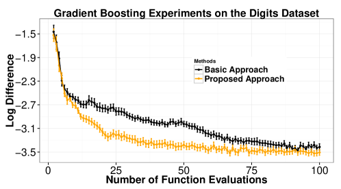
A last batch of experiments considers finding the learning rate and maximum tree depth of a gradient boosting ensemble (Friedman, 2001) of 100 trees that leads to the best performance on the digits dataset from the scikit-learn python package (Pedregosa et al., 2011). We use 70% of the data for training and 30% for validation and compute the performance in terms of the test log-likelihood. We consider optimizing the logarithm of the learning rate and five different values for the maximum depth of the trees. Namely . Again, we report the logarithm of the distance to best observed performance on the validation set. We run each BO method (proposed and basic) for 100 iterations. We consider 100 repetitions of the experiments. The results obtained are displayed in Figure 4. Again, the proposed approach gives better results than the basic approach. More precisely, it is able to find ensembles with better prediction properties on the validation set with a smaller number of evaluations.
5 Conclusions
We have described a new approach to deal with integer-valued variables in BO methods using GPs as the underlying model. This approach consists in (i) rounding real values to integer values and (ii) modifying the covariance function of the GP to account for the fact that the objective should be constant in the interval of all the real values that are rounded to the same integer value. The proposed approach has been evaluated in both synthetic and real problems and compared with a basic approach to handle integer-valued variables. These experiments show that the better modeling properties of the proposed approach lead to better results. More precisely, a BO method using such an approach finds solutions that are closer to the optimal ones in a smaller number of iterations.
Acknowledgments
The authors gratefully acknowledge the use of the facilities of Centro de Computación Científica (CCC) at Universidad Autónoma de Madrid. The authors also acknowledge financial support from Spanish Plan Nacional I+D+i, Grants TIN2013-42351-P, TIN2016-76406-P, TIN2015-70308-REDT and TEC2016-81900-REDT (MINECO/FEDER EU), and from Comunidad de Madrid, Grant S2013/ICE-2845.
References
- Friedman (2001) J. H. Friedman. Greedy function approximation: a gradient boosting machine. Annals of statistics, pages 1189–1232, 2001.
- Jones et al. (1998) D. R. Jones, M. Schonlau, and W. J. Welch. Efficient global optimization of expensive black-box functions. Journal of Global Optimization, 13(4):455–492, 1998.
- Murray and Adams (2010) I. Murray and R. P. Adams. Slice sampling covariance hyperparameters of latent Gaussian models. In Advances in Neural Information Processing Systems 23, pages 1732–1740. 2010.
- Pedregosa et al. (2011) F. Pedregosa, G. Varoquaux, A. Gramfort, V. Michel, B. Thirion, O. Grisel, M. Blondel, P. Prettenhofer, R. Weiss, V. Dubourg, J. Vanderplas, A. Passos, D. Cournapeau, M. Brucher, M. Perrot, and E. Duchesnay. Scikit-learn: Machine learning in Python. Journal of Machine Learning Research, 12:2825–2830, 2011.
- Rasmussen and Williams (2006) C. E. Rasmussen and C. K. I. Williams. Gaussian Processes for Machine Learning (Adaptive Computation and Machine Learning). The MIT Press, 2006. ISBN 026218253X.
- Shahriari et al. (2016) B. Shahriari, K. Swersky, Z. Wang, R. P. Adams, and N. de Freitas. Taking the human out of the loop: A review of Bayesian optimization. Proceedings of the IEEE, 104:148–175, 2016.
- Snoek et al. (2012) J. Snoek, H. Larochelle, and R. P. Adams. Practical Bayesian optimization of machine learning algorithms. In Advances in Neural Information Processing Systems 25, pages 2951–2959. 2012.