Image-Based Prognostics Using Penalized Tensor Regression

Abstract

This paper proposes a new methodology to predict and update the residual useful lifetime of a system using a sequence of degradation images. The methodology integrates tensor linear algebra with traditional location-scale regression widely used in reliability and prognosis. To address the high dimensionality challenge, the degradation image streams are first projected to a low-dimensional tensor subspace that is able to preserve their information. Next, the projected image tensors are regressed against time-to-failure via penalized location-scale tensor regression. The coefficient tensor is then decomposed using CANDECOMP/PARAFAC (CP) and Tucker decompositions, which enables parameter estimation in a high-dimensional setting. Two optimization algorithms with a global convergence property are developed for model estimation. The effectiveness of our models is validated using a simulated dataset and infrared degradation image streams from a rotating machinery.

Keywords: Residual useful lifetimes, penalized tensor regression, (log)-location-scale distribution, image streams

1 Introduction

Imaging is one of the fastest growing technologies for condition monitoring and industrial asset management. Relative to most sensing techniques, industrial imaging devices are easier to use because they are generally noncontact and do not require permanent installation or fixturing. Image data also contains rich information about the object being monitored. Some examples of industrial imaging technologies include infrared images used to measure temperature distributions of equipment and components (Bagavathiappan et al., 2013), charge-coupled device (CCD) images which capture surface quality information (e.g., cracks) of products (Neogi, Mohanta and Dutta, 2014), and others. Image data has been extensively used for process monitoring and diagnostics. For instance, infrared images have been successfully used for civil structures monitoring (Meola, 2007), machinery inspection (Seo et al., 2011), fatigue damage evaluation (Pastor et al., 2008) and electronic printed circuit board (PCB) monitoring (Vellvehi et al., 2011). In steel industry, CCD cameras have been utilized for product surface inspection (Neogi, Mohanta and Dutta, 2014), while video cameras have been used to monitor the shape and color of furnace flames to control quality of steel tubes (Yan, Paynabar and Shi, 2015). This paper expands the utilization of image data by proposing an image-based prognostic modeling framework that uses degradation-based image streams to predict remaining lifetime.

Numerous prognostic methodologies have been developed in the literature. Examples of some modeling approaches include random coefficients models (Gebraeel et al., 2005; Ye and Chen, 2014), models that utilize the Brownian motion process (Ye, Chen and Shen, 2015; Chen et al., 2015) and gamma process (Shu, Feng and Coit, 2015; Zhang and Liao, 2015), and models based on functional data analysis (Fang, Zhou and Gebraeel, 2015; Zhou et al., 2014). These approaches are well-suited for time-series signals, but it is not clear how they can be extended to model image streams. One of the key challenges in modeling image data revolves around the analytical and computational complexities associated with characterizing high dimensional data. High dimensionality arises from the fact that a single image stream consists of a large sequence of images (observed across the life cycle of an equipment) coupled with the large numbers of pixels embedded in each image. Additional challenges are related to the complex spatial-temporal structures inherent in the data streams. Pixels are spatially correlated within a single image and temporally correlated across sequential images. In recent work (Liu, Yeo and Kalagnanam, 2016), degradation image streams were modeled as a spatio-temporal process. Although spatio-temporal models have been widely used to model data with complex spatial and temporal correlation structures (Cressie and Wikle, 2015), they are not necessarily accurate for long-term predictions necessary to our type of prognostic application. Most importantly, a key limitation of spatio-temporal models is that they require a pre-set failure threshold, which is usually hard to define for degradation image streams.

This paper proposes a tensor-based regression framework that utilizes degradation image streams to predict remaining useful life (RUL), and provide advance warning of impending failures of industrial assets. Specifically, we build a (log)-location-scale (LLS) tensor regression model in which the time-to-failure (TTF) is treated as the response and degradation image streams as covariates. LLS regression has been widely used in reliability and survival analysis (Doray, 1994) because it provides a flexible framework capable of modeling a variety of TTF distributions such as (log)normal, (log)logistic, smallest extreme value (SEV), Weibull, etc. To model the spatio-temporal structure of degradation image streams, the regression model treats each image stream as a tensor. A tensor is defined as a multi-dimensional array–a one-order tensor is a vector, a two-order tensor is a matrix, and objects of order three or higher are called high-order tensors. More details about tensor theory and applications can be found in a survey paper by Kolda and Bader (2009). A degradation image stream constitutes a three-order tensor in which the first two dimensions capture the spatial structure of a single image whereas the third dimension is used to model the temporal structure of the image stream. One of the key benefits of modeling a degradation image stream as a tensor is that tensors maintain the spatio-temporal structure within and between images which allows for a relatively accurate RUL prediction model. In this paper, degradation image stream(s) and degradation tensor(s) are used exchangeably hereafter.

The high dimensionality of degradation image streams poses significant computational challenges, especially ones related to parameter estimation. For example, a tensor-regression model for a degradation image stream consisting of 50 images each with $20\times 20$ pixels generates a three-order tensor-coefficient consisting of 20,000 elements that need to be estimated. In an effort to improve model computations, we develop two estimation methods that integrate dimensionality reduction and tensor decomposition. Dimensionality reduction is used as the first step for both estimation methods as it helps reduce the number of parameters. Degradation tensors are projected to a low-dimensional tensor subspace that preserves most of their information. This is achieved using a multilinear dimension reduction technique, such as multilinear principal component analysis (MPCA) (Lu, Plataniotis and Venetsanopoulos, 2008). We utilize the fact that essential information embedded in high-dimensional tensors can be captured in a low-dimensional tensor subspace. Next, the tensor-coefficients corresponding to the projected degradation tensors are decomposed using two popular tensor decomposition approaches namely, CANDECOMP/PARAFAC (CP) (Carroll and Change, 1970) and Tucker (Tucker, 1966). The CP approach decomposes a high-dimensional coefficient tensor as a product of several low-rank basis matrices. In contrast, the Tucker approach expresses the tensor-coefficient as a product of a low-dimensional core tensor and several factor matrices. Therefore, instead of estimating the tensor-coefficient, we only estimate its corresponding core tensors and factor/basis matrices, which significantly reduces the computational complexity and the required sample size. Block relaxation algorithms are also developed for model estimation with guaranteed global convergence to a stationary point.

The remainder of the paper is organized as follows. Section 2 provides an overview of the basic notations and definitions in multilinear algebra. Section 3 presents the degradation and prognostic modeling framework. Section 3.1 and 3.2 discusses the estimation algorithm based on CP decomposition and Tucker decomposition, respectively. In Section 4, we discuss the RUL prediction and realtime updating. The effectiveness of our model is validated using a numerical study in Section 5 and real degradation image streams from a rotating machinery in Section 6. Finally, Section 7 is devoted to concluding remarks.

2 Preliminaries

This section presents some basic notations, definitions and operators in multilinear algebra and tensor analysis that are used throughout the paper. Scalars are denoted by lowercase letters, e.g., $b$, vectors are denoted by lowercase boldface letters, e.g., $\boldsymbol{b}$, matrices are denoted by uppercase boldface letters, e.g., $\boldsymbol{B}$, and tensors are denoted by calligraphic letters, e.g., $\mathcal{B}$. The order of a tensor is the number of modes, also known as way. For example, the order of vectors and matrices are 1 and 2, respectively. A $D$-order tensor is denoted by $\mathcal{B}\in\mathbb{R}^{I_{1}\times\cdots\times I_{D}}$, where $I_{d}$ for $d=1,\ldots,D$ represents the dimension of the $d$-mode of $\mathcal{B}$. The $(i_{1},i_{2},\ldots,i_{D})$-th component of $\mathcal{B}$ is denoted by $b_{i_{1},i_{2},\ldots,i_{D}}$. A fiber of $\mathcal{B}$ is a vector obtained by fixing all indices of $\mathcal{B}$ but one. A vectorization of $\mathcal{B}$, denoted by ${vec}({\mathcal{B}})$, is obtained by stacking all mode-$1$ fibers of ${\mathcal{B}}$. The mode-$d$ matricization of ${\mathcal{B}}$, denoted by $\boldsymbol{B}_{(d)}$, is a matrix whose columns are mode-$d$ fibers of ${\mathcal{B}}$ in the lexicographical order. The mode-$d$ product of a tensor ${\mathcal{B}}\in\mathbb{R}^{I_{1}\times\cdots\times I_{D}}$ with a matrix $A\in\mathbb{R}^{J\times I_{d}}$, denoted by $({\mathcal{B}}\times_{d}A)$, is a tensor whose component is $({\mathcal{B}}\times_{d}A)_{i_{1},\ldots,i_{d-1},j_{d},i_{d+1}\ldots,i_{D}}=\sum_{i_{d}=1}^{I_{d}}b_{i_{1},i_{2},\ldots,i_{D}}a_{j,i_{d}}$. The inner product of two tensors $\mathcal{B}\in\mathbb{R}^{I_{1}\times\cdots\times I_{D}},\mathcal{S}\in\mathbb{R}^{I_{1}\times\cdots\times I_{D}}$ is denoted by $\langle\mathcal{B},\mathcal{S}\rangle=\sum_{i_{1},\ldots,i_{D}}b_{i_{1},\ldots,i_{D}}s_{i_{1},\ldots,i_{D}}$. A rank-one tensor $\mathcal{B}\in\mathbb{R}^{I_{1}\times\cdots\times I_{D}}$ can be represented by outer products of vectors, i.e., $\mathcal{B}=\boldsymbol{b}_{1}\circ\boldsymbol{b}_{2}\circ\cdots\circ\boldsymbol{b}_{D}$, where $\boldsymbol{b}_{d}$ is an $I_{d}$-dimension vector and “$\circ$” is the outer product operator. The Kronecker product of two matrices $\boldsymbol{A}\in\mathbb{R}^{m\times n},\boldsymbol{B}\in\mathbb{R}^{p\times q}$, denoted by $\boldsymbol{A}\otimes\boldsymbol{B}$ is an $mp\times nq$ block matrix defined by

$$M=\left(\begin{smallmatrix}a_{11}\boldsymbol{B}&\ldots&a_{1n}\boldsymbol{B}\\ \vdots&\ddots&\vdots\\ a_{m1}\boldsymbol{B}&\ldots&a_{mn}\boldsymbol{B}\end{smallmatrix}\right).$$

The Khatri-Rao product of two matrices $\boldsymbol{A}\in\mathbb{R}^{m\times r},\boldsymbol{B}\in\mathbb{R}^{p\times r}$, denoted by $\boldsymbol{A}\odot\boldsymbol{B}$, is a $mp\times r$ matrix defined by $\left[\boldsymbol{a}_{1}\otimes\boldsymbol{b}_{1}\;\;\boldsymbol{a}_{2}\otimes\boldsymbol{b}_{2}\;\;\cdots\;\;\boldsymbol{a}_{r}\otimes\boldsymbol{b}_{r}\right]$, where $\boldsymbol{a}_{i}\in\mathbb{R}^{m\times 1}$, and $\boldsymbol{b}_{i}\in\mathbb{R}^{p\times 1}$ for $i=1,\ldots,r$.

3 Prognostic Modeling Using Degradation Tensors

This paper considers engineering systems with degradation process that can be represented by tensors, e.g., degradation image streams or profiles. The underlying premise of our prognostic modeling framework rests on using LLS regression to model TTF as a function of degradation tensors. One of the main challenges in fitting such regression models is the high-dimensionality of data which makes coefficients estimation intractable. To address this issue, we use the fact that the essential information of high-dimensional data is often embedded in a low-dimensional subspace. Specifically, we project degradation and coefficient tensors onto a low-dimensional tensor subspace that preserves their inherent information.

To further reduce the number of estimated parameters, coefficient tensors are decomposed using two widely used tensor decomposition techniques, CP and Tucker. The CP decomposition expresses a high-dimensional coefficient tensor as a product of several smaller sized basis matrices (Carroll and Change, 1970). Tucker decomposition, however, expresses a high-dimensional coefficient tensor as a product of a low-dimensional core tensor and several factor matrices (Tucker, 1966). Thus, instead of estimating the coefficient tensor, we only need to estimate its corresponding core tensors and factor/basis matrices, which significantly helps reduce the computational complexity and the required sample for estimation. The parameters of the reduced LLS regression model are estimated using the maximum likelihood (ML) approach. To obtain the ML estimates, we propose optimization algorithms for CP-based and Tucker-based methods . The optimization algorithms are based on the block relaxation method (De Leeuw, 1994; Lange, 2010), which alternately updates one block of the parameters while keeping other parameters fixed. Finally, the estimated LLS regression is used to predict and update the RUL of a functioning system. In the following, the details of the proposed methodology is presented.

Our framework is applicable in settings that have a historical dataset of degradation image streams (i.e., degradation tensor) for a sample of units with corresponding TTFs. Let $N$ denote the number of units that make up the historical (training) sample. Let $\mathcal{S}_{i}\in\mathbb{R}^{I_{1}\times\cdots\times I_{D}}$, for $i=1,\ldots,N$, denote the degradation tensor and $\tilde{y}_{i}$ represent the TTF. The following LLS regression model expresses the TTF as a function of a degradation tensor:

$$y_{i}=\alpha+\langle\mathcal{B},\mathcal{S}_{i}\rangle+\sigma\epsilon_{i}$$ (1)

where $y_{i}=\tilde{y}_{i}$ for a location-scale model and $y_{i}=\ln(\tilde{y}_{i})$ for a log-location-scale model, the scalar $\alpha$ is the intercept of the regression model, and $\mathcal{B}\in\mathbb{R}^{I_{1}\times\cdots\times I_{D}}$ is the tensor of regression coefficients. $\alpha+\langle\mathcal{B},\mathcal{S}_{i}\rangle$ is known as the location parameter and $\sigma$ is the scale parameter. Similar to common LLS regression models (Doray, 1994), we assume that only the location parameter is a function of the covariates, i.e., the degradation tensor. The term $\epsilon_{i}$ is the random noise term with a standard location-scale density $f(\epsilon)$. For example, $f(\epsilon)=\exp(\epsilon-\exp(\epsilon))$ for SEV distribution, $f(\epsilon)=\exp(\epsilon)/(1+\exp(\epsilon))^{2}$ for logistic distribution, and $f(\epsilon)=1/\sqrt{2\pi}\exp(-\epsilon^{2}/2)$ for normal distribution. Consequently, $y_{i}$ has a density in the form of $\frac{1}{\sigma}f\left(\frac{y_{i}-\alpha-\langle\mathcal{B},\mathcal{S}_{i}\rangle}{\sigma}\right)$.

The number of parameters in Model (1) is given by $2+\prod_{d=1}^{D}I_{d}$. Recall that $I_{d}$ for $d=1,\ldots,D$ represents the dimension of the $d$-mode of $\mathcal{B}$. If we consider a simple example of an image stream constituting 100 images of size $40\times 50$, i.e., $\mathcal{S}_{i}$ is a 3-order tensor in $\mathbb{R}^{40\times 50\times 100}$, the number of parameters to be estimated will be quite large: $200,002=2+40\times 50\times 100$. To reduce the number of parameters, as mentioned earlier, we project the degradation tensors and the coefficient tensor onto a low-dimensional tensor subspace that captures the relevant information of the degradation tensors. The following proposition shows that by using multilinear dimension reduction techniques, we can significantly reduce the dimensions of the coefficient tensor without significant loss of information.

Proposition 1.

Suppose $\{\mathcal{S}_{i}\}_{i=1}^{N}$ can be expanded by $\mathcal{S}_{i}=\tilde{\mathcal{S}}_{i}\times_{1}\boldsymbol{U}_{1}\times_{2}\boldsymbol{U}_{2}\times\cdots\times_{D}\boldsymbol{U}_{D}$, where $\tilde{\mathcal{S}}_{i}\in\mathbb{R}^{P_{1}\times\cdots\times P_{D}}$ is a low-dimensional tensor and matrices $\boldsymbol{U}_{d}\in\mathbb{R}^{P_{d}\times I_{d}}$, $\boldsymbol{U}_{d}^{\top}\boldsymbol{U}_{d}=\boldsymbol{I}_{I_{d}}$, $P_{d}<I_{d}$, $d=1,\ldots,D$. If the coefficient tensor, $\mathcal{B}$, is projected onto the tensor subspace spanned by $\{\boldsymbol{U}_{1},\ldots,\boldsymbol{U}_{D}\}$, i.e., $\tilde{\mathcal{B}}=\mathcal{B}\times_{1}\boldsymbol{U}_{1}^{\top}\times_{2}\boldsymbol{U}_{2}^{\top}\times\cdots\times_{D}\boldsymbol{U}_{D}^{\top}$, where $\tilde{\mathcal{B}}$ is the projected coefficient tensor, then $\langle\mathcal{B},\mathcal{S}_{i}\rangle=\langle\tilde{\mathcal{B}},\tilde{\mathcal{S}}_{i}\rangle$.

The proof of Proposition 1 is given in Appendix A. Proposition 1 implies that the original high-dimensional tensors, (i.e., $\mathcal{B}$ and $\mathcal{S}$) and their corresponding low-rank projections (i.e., $\tilde{\mathcal{B}}$ and $\tilde{\mathcal{S}}_{i}$) result in similar estimates of the location parameter. Using Proposition 1, we can re-express Equation (1) as follows:

$$y_{i}=\alpha+\langle\tilde{\mathcal{B}},\tilde{\mathcal{S}}_{i}\rangle+\sigma\epsilon_{i}.$$ (2)

The low-dimensional tensor space defined by factor matrices $\boldsymbol{U}_{d}\in\mathbb{R}^{P_{d}\times I_{d}}$ can be obtained by applying multilinear dimension reduction techniques, such as multilinear principal component analysis (MPCA) (Lu, Plataniotis and Venetsanopoulos, 2008), on the training degradation tensor, $\{\mathcal{S}_{i}\}_{i=1}^{N}$. The objective of MPCA is to find a set of orthogonal factor matrices $\{\boldsymbol{U}_{d}\in\mathbb{R}^{P_{d}\times I_{d}},\boldsymbol{U}_{d}^{\top}\boldsymbol{U}_{d}=\boldsymbol{I}_{I_{d}},P_{d}<I_{d}\}_{d=1}^{D}$ such that the projected low-dimensional tensor captures most of the variation in the original tensor. Mathematically, this can be formalized into the following optimization problem:

$$\{\boldsymbol{U}_{1},\ldots,\boldsymbol{U}_{D}\}=\operatorname*{arg\,max}_{\boldsymbol{U}_{1},\ldots,\boldsymbol{U}_{D}}\sum_{i=1}^{N}\left\|(\mathcal{S}_{i}-\bar{\mathcal{S}})\times_{1}\boldsymbol{U}_{1}^{\top}\times_{2}\boldsymbol{U}_{2}^{\top}\times\cdots\times_{D}\boldsymbol{U}_{D}^{\top}\right\|_{F}^{2}$$ (3)

where $\bar{\mathcal{S}}=\frac{1}{N}\sum_{i=1}^{N}\mathcal{S}_{i}$ is the mean tensor. This optimization problem can be solved iteratively using the algorithm given in Appendix B. Additional details regarding the algorithm and the methods used to determine the dimensionality of the tensor subspace, $\{P_{d}\}_{d=1}^{D}$, can be found in Lu, Plataniotis and Venetsanopoulos (2008). This approach helps to reduce the number of parameters to be estimated from $2+\prod_{d=1}^{D}I_{d}$ in Equation (1) to $2+\prod_{d=1}^{D}P_{d}$ in Equation (2) where $2+\prod_{d=1}^{D}P_{d}<<2+\prod_{d=1}^{D}I_{d}$.

However, often, the number of reduced parameters (i.e., $2+\prod_{d=1}^{D}P_{d}$) is still so large that requires further dimension reduction. For example, for a $40\times 50\times 100$ tensor, if $P_{1}=P_{2}=P_{3}=10$, the number of parameters is reduced from 200,002 to 1,002. To further reduce the number of parameters so that they can be estimated by using a limited training sample, we utilize two well-known tensor decomposition techniques namely, CP and Tucker decompositions. We briefly review these decompositions in Sections 3.1 and 3.2, and discuss how they are incorporated into our prognostic framework.

3.1 Dimension Reduction via CP Decomposition

In CP decomposition, the coefficient tensor $\tilde{\mathcal{B}}$ in Equation (2) is decomposed into a sum product of a set of rank one vectors. Given the rank of $\tilde{\mathcal{B}}$, which we denote by $R$, we have the following decomposition,

$$\tilde{\mathcal{B}}=\sum_{r=1}^{R}\tilde{\boldsymbol{\beta}}_{1}^{(r)}\circ\cdots\circ\tilde{\boldsymbol{\beta}}_{D}^{(r)},$$ (4)

where $\tilde{\boldsymbol{\beta}}_{d}^{(r)}=\left[\tilde{\beta}_{d,1}^{(r)},\ldots,\tilde{\beta}_{d,P_{d}}^{(r)}\right]^{\top}\in\mathbb{R}^{P_{d}}$, and “$\circ$” denotes the outer product operator. It can be easily shown that ${vec}(\tilde{\mathcal{B}})=(\tilde{\boldsymbol{B}}_{D}\odot\cdots\odot\tilde{\boldsymbol{B}}_{1})\boldsymbol{1}_{R}$, where $\tilde{\boldsymbol{B}}_{d}=\left[\tilde{\boldsymbol{\beta}}_{d}^{(1)},\ldots,\tilde{\boldsymbol{\beta}}_{d}^{(R)}\right]\in\mathbb{R}^{P_{d}\times R}$ for $d=1,\ldots,D$ and $\boldsymbol{1}_{R}\in\mathbb{R}^{R}$ is an $R$ dimensional vector of ones. Thus, Equation (2) can be re-expressed as follows:

$$\begin{split}y_{i}&=\alpha+\left\langle{vec}(\tilde{\mathcal{B}}),{vec}(\tilde{\mathcal{S}}_{i})\right\rangle+\sigma\epsilon_{i}\\ &=\alpha+\left\langle(\tilde{\boldsymbol{B}}_{D}\odot\cdots\odot\tilde{\boldsymbol{B}}_{1})\boldsymbol{1}_{R},{vec}(\tilde{\mathcal{S}}_{i})\right\rangle+\sigma\epsilon_{i}\\ \\ \end{split}$$ (5)

The number of parameters in Equation (5) is $2+\sum_{d=1}^{D}P_{d}\times R$, which is significantly smaller than $2+\prod_{d=1}^{D}P_{d}$ from (2). In our 3-order tensor example, if $P_{1}=P_{2}=P_{3}=10$ and the rank $R=2$, the number of parameters decreases from $1,002$ to $62=2+10\times 2+10\times 2+10\times 2$.

3.1.1 Parameter Estimation for CP Decomposition

To estimate the parameters of Equation (5) using MLE, we maximize the corresponding penalized log-likelihood function:

$$\operatorname*{arg\,max}_{\boldsymbol{\theta}}\left\{\ell(\boldsymbol{\theta})-\sum_{d=1}^{D}r\left(\tilde{\boldsymbol{B}}_{d}\right)\right\}$$

$$= \operatorname*{arg\,max}_{\boldsymbol{\theta}}\left\{-N\log\sigma+\sum_{i=1}^{N}\log f\left(\frac{y_{i}-\alpha-\left\langle(\tilde{\boldsymbol{B}}_{D}\odot\cdots\odot\tilde{\boldsymbol{B}}_{1})\boldsymbol{1}_{R},{vec}(\tilde{\mathcal{S}}_{i})\right\rangle}{\sigma}\right)\right.$$

$$\left.-\sum_{d=1}^{D}r\left(\tilde{\boldsymbol{B}}_{d}\right)\right\}$$ (6)

where $\boldsymbol{\theta}=(\alpha,\sigma,\tilde{\boldsymbol{B}}_{1}\ldots,\tilde{\boldsymbol{B}}_{D})$ and $r(\tilde{\boldsymbol{B}}_{d})=\lambda_{d}\sum_{r=1}^{R}\sum_{j=1}^{P_{d}}\|\tilde{\beta}_{d,j}^{(r)}\|_{1}$. The $\ell_{1}$-norm penalty term encourages the sparsity of $\tilde{\mathcal{B}}$, which helps avoid over-fitting.

The block relaxation method proposed by (De Leeuw, 1994; Lange, 2010) is used to maximize expression (3.1.1). Specifically, we iteratively update a block of parameters, say $(\tilde{\boldsymbol{B}}_{d},\sigma,\alpha)$, while keeping other components $\{\tilde{\boldsymbol{B}}_{1},\ldots,\tilde{\boldsymbol{B}}_{d-1},\tilde{\boldsymbol{B}}_{d+1},\ldots,\tilde{\boldsymbol{B}}_{D}\}$ fixed. In each update, the optimization criterion is reduced to $\operatorname*{arg\,max}_{\boldsymbol{\tilde{B}}_{d},\sigma,\alpha}\left\{\ell(\boldsymbol{\theta})-r(\tilde{\boldsymbol{B}}_{d})\right\}$.

Next, we show in Proposition 2 that the optimization problem for each block $\tilde{\boldsymbol{B}}_{d}$ is equivalent to optimizing the penalized log-likelihood function for $y_{i}=\alpha+\langle\tilde{\boldsymbol{B}}_{d},\boldsymbol{X}_{d,i}\rangle+\sigma\epsilon_{i}$, where $\tilde{\boldsymbol{B}}_{d}$ is the parameter matrix and $\boldsymbol{X}_{d,i}$ is the predictor matrix defined by $\boldsymbol{X}_{d,i}=\tilde{\boldsymbol{S}}_{i(d)}(\tilde{\boldsymbol{B}}_{D}\odot\cdots\odot\tilde{\boldsymbol{B}}_{d+1}\odot\tilde{\boldsymbol{B}}_{d-1}\odot\cdots\odot\tilde{\boldsymbol{B}}_{1})$, and where $\tilde{\boldsymbol{S}}_{i(d)}$ is the mode-d matricization of $\tilde{\mathcal{S}}_{i}$ (defined in the Preliminaries Section).

Proposition 2.

Consider the optimization problem in (3.1.1), given $(\tilde{\boldsymbol{B}}_{1},\ldots,\tilde{\boldsymbol{B}}_{d-1},\tilde{\boldsymbol{B}}_{d+1},\ldots,\tilde{\boldsymbol{B}}_{D})$, the optimization problem can be reduced to

$$\operatorname*{arg\,max}_{\boldsymbol{\tilde{B}}_{d},\sigma,\alpha}\left\{-N\ln\sigma+\sum_{i=1}^{N}\ln f\left(\frac{y_{i}-\alpha-\left\langle\tilde{\boldsymbol{B}}_{d},\boldsymbol{X}_{d,i}\right\rangle}{\sigma}\right)-r(\tilde{\boldsymbol{B}}_{d})\right\}.$$ (7)

The proof of Proposition 2 is provided in Appendix C. As pointed out by Städler, Bühlmann and Geer (2010), the estimates of $\alpha,\boldsymbol{\tilde{B}}_{d},\sigma$ in optimizing problem (7) are not invariant under scaling of the response. To be specific, consider the transformation $y_{i}^{\prime}=by_{i},\alpha^{\prime}=b\alpha,\tilde{\boldsymbol{B}}_{d}^{\prime}=b\tilde{\boldsymbol{B}_{d}},\sigma^{\prime}=b\sigma$ where $b>0$. Clearly, this transformation does not affect the regression model $y_{i}=\alpha+\langle\tilde{\boldsymbol{B}}_{d},\boldsymbol{X}_{d,i}\rangle+\sigma\epsilon_{i}$. Therefore, invariant estimates based on the transformed data $(y_{i}^{\prime},\boldsymbol{X}_{d,i})$, should satisfy $\hat{\alpha}^{\prime}=b\hat{\alpha},\hat{\tilde{\boldsymbol{B}}}_{d}^{\prime}=b\hat{\tilde{\boldsymbol{B}}}_{d},\hat{\sigma}^{\prime}=b\hat{\sigma}$, where $\hat{\alpha},\hat{\tilde{\boldsymbol{B}}}_{d},\hat{\sigma}$ are estimates based on original data $(y_{i},\boldsymbol{X}_{d,i})$. However, this does not hold for the estimates obtained by optimizing (7). To address this issue, expression (7) is modified by dividing the penalty term by the scale parameter $\sigma$:

$$\operatorname*{arg\,max}_{\boldsymbol{\tilde{B}}_{d},\sigma,\alpha}\left\{-N\ln\sigma+\sum_{i=1}^{N}\ln f\left(\frac{y_{i}-\alpha-\left\langle\tilde{\boldsymbol{B}}_{d},\boldsymbol{X}_{d,i}\right\rangle}{\sigma}\right)-r(\frac{\tilde{\boldsymbol{B}}_{d}}{\sigma})\right\}.$$ (8)

We can show that the resulting estimates possess the invariant property (see Appendix D). Note that in the modified problem, the penalty term penalizes the $\ell_{1}$-norm of the coefficients and the scale parameter $\sigma$ simultaneously, which has some close relations to the Bayesian Lasso (Park and Casella, 2008; Städler, Bühlmann and Geer, 2010). The log-likelihood function in (8) is not concave which causes computational problems. We use the following re-parameterization to transform the optimization function to a concave function: $\alpha_{0}=\alpha/\sigma,\boldsymbol{A}_{d}=\tilde{\boldsymbol{B}}_{d}/\sigma,\rho=1/\sigma$. Consequently, the optimization problem can be rewritten as:

$$\operatorname*{arg\,max}_{\boldsymbol{A}_{d},\rho,\alpha_{0}}\left\{N\ln\rho+\sum_{i=1}^{N}\ln f\left(\rho y_{i}-\alpha_{0}-\left\langle\boldsymbol{A}_{d},\boldsymbol{X}_{d,i}\right\rangle\right)-r(\boldsymbol{A}_{d})\right\}.$$ (9)

The optimization problem in (9) is concave if function $f$ is log-concave, which is the case for most LLS distributions including normal, logistic, SEV, generalized log-gamma, log-inverse Gaussian (Doray, 1994). Lognormal, log-logistic and Weibull distributions whose density function is not log-concave can easily be transformed to normal, logistic and SEV distributions, respectively, by taking the logarithm of the TTF. Various optimization algorithms such as coordinate descent (Friedman et al., 2007) and gradient descent (Tseng, 2001) can be used for solving (9). Algorithm 1 shows the steps of the block relaxation method for optimizing (9) and finding the ML estimates of the parameters.

Algorithm 1: Block relaxation algorithm for solving problem (3.1.1).
Input: $\{\tilde{\mathcal{S}_{i}},y_{i}\}_{i=1}^{N}$ and rank $R$
Initialization: Matrices $\tilde{\boldsymbol{B}}_{2}^{(0)},\tilde{\boldsymbol{B}}_{3}^{(0)},\ldots,\tilde{\boldsymbol{B}}_{D}^{(0)}$ are initialized randomly.
while convergence criterion not met do
for $d=1,\ldots,D$ do
$\boldsymbol{X}_{d,i}^{(k+1)}=\tilde{\boldsymbol{S}}_{i(d)}(\tilde{\boldsymbol{B}}_{D}^{(k)}\odot\cdots\odot\tilde{\boldsymbol{B}}_{d+1}^{(k)}\odot\tilde{\boldsymbol{B}}_{d-1}^{(k+1)}\odot\cdots\odot\tilde{\boldsymbol{B}}_{1}^{(k+1)})$
$\begin{aligned} \boldsymbol{A}_{d}^{(k+1)},\rho^{(k+1)},\alpha_{0}^{(k+1)}=\operatorname*{arg\,max}_{\boldsymbol{A}_{d},\rho,\alpha_{0}}\{N\ln\rho+\sum_{i=1}^{N}\ln f(\rho y_{i}-\alpha_{0}-\langle\boldsymbol{A}_{d},\boldsymbol{X}_{d,i}^{(k+1)}\rangle)-r(\boldsymbol{A}_{d})\}\end{aligned}$
$\tilde{\boldsymbol{B}}_{d}^{(k+1)}=\boldsymbol{A}_{d}^{(k+1)}/\rho^{(k+1)}$
end for
Let $k=k+1$
end while
Output:$\alpha=\alpha_{0}/\rho,\sigma=1/\rho,\{\tilde{\boldsymbol{B}}_{d}\}_{d=1}^{D}$

The convergence criterion is defined by $\ell(\tilde{\boldsymbol{\theta}}^{(k+1)})-\ell(\tilde{\boldsymbol{\theta}}^{(k)})<\epsilon$, in which $\ell(\tilde{\boldsymbol{\theta}}^{(k)})$, is defined as follows:

$$\ell(\tilde{\boldsymbol{\theta}}^{(k)})=-N\log\sigma^{(k)}+\sum_{i=1}^{N}\log f\left(\frac{y_{i}-\alpha^{(k)}-\left\langle(\tilde{\boldsymbol{B}}_{D}^{(k)}\odot\cdots\odot\tilde{\boldsymbol{B}}_{1}^{(k)})\boldsymbol{1}_{R},{vec}(\tilde{\mathcal{S}}_{i})\right\rangle}{\sigma^{(k)}}\right)$$ (10)

$$-\sum_{d=1}^{D}r\left(\frac{\tilde{\boldsymbol{B}}_{d}^{(k)}}{\sigma^{(k)}}\right)$$

where $\tilde{\boldsymbol{\theta}}^{(k)}=(\alpha^{(k)},\sigma^{(k)},\tilde{\boldsymbol{B}}_{1}^{(k)},\ldots,\tilde{\boldsymbol{B}}_{D}^{(k)})$.

It can be shown that Algorithm 1 exhibits the global convergence property (see Proposition 1 in Zhou, Li and Zhu (2013)). In other words, it will converge to a stationary point for any initial point. Since a stationary point is only guaranteed to be a local maximum or saddle point, the algorithm is run several times with different initializations while recording the best results.

Algorithm 1 requires the rank of $\tilde{\mathcal{B}}$ to be known a priori for CP decomposition. In this paper, the Bayesian information criterion (BIC) is used to determine the appropriate rank. The BIC is defined as $-2\ell(\tilde{\boldsymbol{\theta}})+P\ln(N)$, where $\ell$ is the log-likelihood value defined in Equation (10), $N$ is the sample size (number of systems) and $P$ is the number of effective parameters. For $D=2$, we set $P=R(P_{1}+P_{2})-R^{2}$, where $-R^{2}$ is used for adjustment of the nonsingular transformation indeterminacy for model identifiability; for $D>2$, we set $P=R(\sum_{d=1}^{D}P_{d}-D+1)$, where $R(-D+1)$ is used for the scaling indeterminacy in the CP decomposition (Li, Zhou and Li, 2013).

3.2 Dimension Reduction via Tucker decomposition

Tucker decomposition is the second tensor decomposition approach used in this paper. It is used to reduce the dimensionality of $\tilde{\mathcal{B}}$ as a product of a low-dimensional core tensor and a set of factor matrices as follows:

$$\tilde{\mathcal{B}}=\mathcal{\tilde{G}}\times_{1}\tilde{\boldsymbol{B}}_{1}\times_{2}\tilde{\boldsymbol{B}}_{2}\times_{3}\cdots\times_{D}\tilde{\boldsymbol{B}}_{D}=\sum_{r_{1}=1}^{R_{1}}\cdots\sum_{r_{D}=1}^{R_{D}}\tilde{g}_{r_{1},\ldots,r_{D}}\tilde{\boldsymbol{\beta}}_{1}^{(r_{1})}\circ\cdots\circ\tilde{\boldsymbol{\beta}}_{D}^{(r_{D})},$$ (11)

where $\mathcal{\tilde{G}}\in\mathbb{R}^{R_{1}\times R_{2}\times\cdots\times R_{D}}$ is the core tensor with element $(\tilde{\mathcal{G}})_{r_{1},\ldots,r_{D}}=\tilde{g}_{r_{1},\ldots,r_{D}}$, $\tilde{\boldsymbol{B}}_{d}=\left[\tilde{\boldsymbol{\beta}}_{d}^{(1)},\ldots,\tilde{\boldsymbol{\beta}}_{d}^{(R_{d})}\right]\in\mathbb{R}^{P_{d}\times R_{d}}$ for $d=1,\ldots,D$ is the factor matrix, “$\times_{d}$” is the mode-$d$ product operator, and “$\circ$” is the outer product operator. Using this decomposition, Equation (2) can be re-expressed as follows:

$$\begin{split}y_{i}&=\alpha+\langle\tilde{\mathcal{B}},\tilde{\mathcal{S}}_{i}\rangle+\sigma\epsilon_{i}\\ &=\alpha+\langle\mathcal{\tilde{G}}\times_{1}\tilde{\boldsymbol{B}}_{1}\times_{2}\tilde{\boldsymbol{B}}_{2}\times_{3}\cdots\times_{D}\tilde{\boldsymbol{B}}_{D},\tilde{\mathcal{S}}_{i}\rangle+\sigma\epsilon_{i}\end{split}$$ (12)

3.2.1 Parameter Estimation for Tucker Decomposition

The following penalized log-likelihood function is used to compute the MLE estimates of the parameters in expression (12).

$$\operatorname*{arg\,max}_{\boldsymbol{\theta}}\left\{\ell(\boldsymbol{\theta})-r(\mathcal{\mathcal{\tilde{G}}})-\sum_{d=1}^{D}r\left(\tilde{\boldsymbol{B}}_{d}\right)\right\}$$

$$= \operatorname*{arg\,max}_{\boldsymbol{\theta}}\left\{-N\ln\sigma+\sum_{i=1}^{N}\ln f\left(\frac{y_{i}-\alpha-\left\langle\mathcal{\tilde{G}}\times_{1}\tilde{\boldsymbol{B}}_{1}\times_{2}\tilde{\boldsymbol{B}}_{2}\times_{3}\cdots\times_{D}\tilde{\boldsymbol{B}}_{D},\tilde{\mathcal{S}}_{i}\right\rangle}{\sigma}\right)\right.$$

$$\left.-r(\mathcal{\mathcal{\tilde{G}}})-\sum_{d=1}^{D}r\left(\tilde{\boldsymbol{B}}_{d}\right)\right\},$$ (13)

where $\boldsymbol{\theta}=(\alpha,\sigma,\mathcal{\mathcal{\tilde{G}}},\tilde{\boldsymbol{B}}_{1},\ldots,\tilde{\boldsymbol{B}}_{D})$, $r(\mathcal{\mathcal{\mathcal{\tilde{G}}}})=\lambda\sum_{r_{1}=1}^{R_{1}}\cdots\sum_{r_{D}=1}^{R_{D}}\|\tilde{g}_{r_{1},\ldots,r_{D}}\|_{1}$ and  $r(\tilde{\boldsymbol{B}}_{d})=\lambda_{d}\sum_{r_{d}=1}^{R_{d}}\sum_{j=1}^{P_{d}}\|\tilde{\beta}_{d,j}^{(r_{d})}\|_{1}$.

Similar to the CP decomposition model, the block relaxation method is used to solve expression (13). To update the core tensor $\mathcal{\mathcal{\tilde{G}}}$ given all the factor matrices, the optimization criterion is reduced to $\operatorname*{arg\,max}_{\mathcal{\tilde{G}}}\left\{\ell(\boldsymbol{\theta})-r(\mathcal{\mathcal{\tilde{G}}})\right\}.$ Proposition 3 shows that this optimization problem is equivalent to optimizing the penalized log-likelihood function of $y_{i}=\alpha+\langle vec(\mathcal{\mathcal{\mathcal{\tilde{G}}}}),\boldsymbol{x}_{i}\rangle+\sigma\epsilon_{i}$, where $vec(\mathcal{\mathcal{\mathcal{\tilde{G}}}})$ is the parameter vector and $\boldsymbol{x}_{i}$ is the predictor vector defined by $\boldsymbol{x}_{i}=(\tilde{\boldsymbol{B}}_{D}\otimes\cdots\otimes\tilde{\boldsymbol{B}}_{1})^{\top}vec(\tilde{\mathcal{S}}_{i})$.

Proposition 3.

Consider the optimization problem in (13), given $\{\tilde{\boldsymbol{B}}_{1},\ldots,\tilde{\boldsymbol{B}}_{D}\}$, the optimization problem is reduced to

$$\operatorname*{arg\,max}_{\mathcal{\mathcal{\mathcal{\mathcal{\tilde{G}}}}}}\left\{-N\ln\sigma+\sum_{i=1}^{N}\ln f\left(\frac{y_{i}-\alpha-\left\langle vec(\mathcal{\mathcal{\mathcal{\mathcal{\tilde{G}}}}}),(\tilde{\boldsymbol{B}}_{D}\otimes\cdots\otimes\tilde{\boldsymbol{B}}_{1})^{\top}vec(\tilde{\mathcal{S}}_{i})\right\rangle}{\sigma}\right)-r(\mathcal{\mathcal{\mathcal{\mathcal{\tilde{G}}}}})\right\},$$ (14)

The proof of Proposition 3 is given in Appendix E. To guarantee the invariance property of the estimates and concavity of the optimization function, we apply the following reparameterization: $\rho=1/\sigma,\alpha_{0}=\alpha/\sigma,\mathcal{C}=\mathcal{\tilde{\mathcal{G}}}/\sigma$,$r(\mathcal{C})=\lambda\sum_{r_{1}=1}^{R_{1}}\cdots\sum_{r_{D}=1}^{R_{D}}\frac{\|\tilde{g}_{r_{1},\ldots,r_{D}}\|_{1}}{\sigma}$. This enables us to re-express criterion (14) as follows:

$$\operatorname*{arg\,max}_{\mathcal{C},\rho,\alpha_{0}}\left\{N\ln\rho+\sum_{i=1}^{N}\ln f\left(\rho y_{i}-\alpha_{0}-\left\langle vec(\mathcal{C}),(\tilde{\boldsymbol{B}}_{D}\otimes\cdots\otimes\tilde{\boldsymbol{B}}_{1})^{\top}vec(\tilde{\mathcal{S}}_{i})\right\rangle\right)-r(\mathcal{C})\right\}.$$ (15)

To update the factor matrix $\tilde{\boldsymbol{B}}_{d}$ for $d=1,\ldots,D$, we fix the core tensor $\mathcal{\mathcal{\tilde{\mathcal{G}}}}$ and the rest of the factor matrices $\{\tilde{\boldsymbol{B}}_{1},\ldots,\tilde{\boldsymbol{B}}_{d-1},\tilde{\boldsymbol{B}}_{d+1}\ldots,\tilde{\boldsymbol{B}}_{D}\}$, and maximize the following criterion $\operatorname*{arg\,max}_{\tilde{\boldsymbol{B}}_{d}}\left\{\ell(\boldsymbol{\theta})-r(\tilde{\boldsymbol{B}}_{d})\right\}$. Proposition 4 shows that this optimization problem is equivalent to optimizing the log-likelihood function of $y_{i}=\alpha+\langle\tilde{\boldsymbol{B}}_{d},\boldsymbol{X}_{d,i}\rangle+\sigma\epsilon_{i},$where $\tilde{\boldsymbol{B}}_{d}$ is the parameter matrix and $\boldsymbol{X}_{d,i}$ is the predictor matrix defined by $\boldsymbol{X}_{d,i}=\tilde{\boldsymbol{S}}_{i(d)}(\tilde{\boldsymbol{B}}_{D}\otimes\cdots\otimes\tilde{\boldsymbol{B}}_{d+1}\otimes\tilde{\boldsymbol{B}}_{d-1}\otimes\cdots\otimes\tilde{\boldsymbol{B}}_{1})\tilde{\boldsymbol{G}}_{(d)}^{\top}$, where $\tilde{\boldsymbol{S}}_{i(d)}$ and $\tilde{\boldsymbol{G}}_{(d)}$ are the mode-d matricization of $\tilde{\mathcal{S}_{i}}$ and $\tilde{\mathcal{G}}$, respectively.

Proposition 4.

Consider the problem in (13), given $\mathcal{\tilde{G}}$ and $\{\tilde{\boldsymbol{B}}_{1},\ldots,\tilde{\boldsymbol{B}}_{d-1},\tilde{\boldsymbol{B}}_{d+1},\ldots,\tilde{\boldsymbol{B}}_{D}\}$, the optimization problem is reduced to

$$\operatorname*{arg\,max}_{\tilde{\boldsymbol{B}}_{d}}\left\{-N\ln\sigma+\sum_{i=1}^{N}\ln f\left(\frac{y_{i}-\alpha-\left\langle\tilde{\boldsymbol{B}}_{d},\boldsymbol{X}_{d,i}\right\rangle}{\sigma}\right)-r(\tilde{\boldsymbol{B}}_{d})\right\}.$$ (16)

The proof of Proposition 4 is provided in Appendix F. Similar to expression (8), we use penalty term $r(\frac{\tilde{\boldsymbol{B}}_{d}}{\sigma})$ and let $\rho=1/\sigma,\alpha_{0}=\alpha/\sigma,\boldsymbol{A}_{d}=\tilde{\boldsymbol{B}}_{d}/\sigma$. Consequently, we obtain the following optimization subproblem for parameter estimation:

$$\operatorname*{arg\,max}_{\boldsymbol{A}_{d}}\left\{N\ln\rho+\sum_{i=1}^{N}\ln f\left(\rho y_{i}-\alpha_{0}-\left\langle\boldsymbol{A}_{d},\boldsymbol{X}_{d,i}\right\rangle\right)-r(\boldsymbol{A}_{d})\right\}.$$ (17)

Algorithm 2: Block relaxation algorithm for solving problem (12).

Input: $\{\tilde{\mathcal{S}_{i}},y_{i}\}_{i=1}^{N}$ and rank $\{R_{d}\}_{d=1}^{D}$

Initialization: Core tensor $\mathcal{G}^{(0)}$ and matrices $\tilde{\boldsymbol{B}}_{2}^{(0)},\tilde{\boldsymbol{B}}_{3}^{(0)},\ldots,\tilde{\boldsymbol{B}}_{D}^{(0)}$ are initialized randomly.

while convergence criterion not met do

for $d=1,\ldots,D$ do

$\boldsymbol{X}_{d,i}^{(k+1)}=\tilde{\boldsymbol{S}}_{i(d)}(\tilde{\boldsymbol{B}}_{D}^{(k)}\otimes\cdots\otimes\tilde{\boldsymbol{B}}_{d+1}^{(k)}\otimes\tilde{\boldsymbol{B}}_{d-1}^{(k+1)}\otimes\cdots\otimes\tilde{\boldsymbol{B}}_{1}^{(k+1)})\{\boldsymbol{G}_{(d)}^{(k)}\}^{\top}$

$\begin{aligned} \boldsymbol{A}_{d}^{(k+1)},\rho^{(k+1)},\alpha_{0}^{(k+1)}=\operatorname*{arg\,max}_{\boldsymbol{A}_{d},\rho,\alpha_{0}}\{N\ln\rho+\sum_{i=1}^{N}\ln f(\rho y_{i}-\alpha_{0}-\langle\boldsymbol{A}_{d},\boldsymbol{X}_{d,i}^{(k+1)}\rangle)-r(\boldsymbol{A}_{d})\}\end{aligned}$

$\tilde{\boldsymbol{B}}_{d}^{(k+1)}=\boldsymbol{A}_{d}^{(k+1)}/\rho^{(k+1)}$

end for

$\begin{aligned} \mathcal{C}^{(k+1)},\rho^{(k+1)},\alpha_{0}^{(k+1)}=\operatorname*{arg\,max}_{\mathcal{C},\rho,\alpha_{0}}\{N\ln\rho+\sum_{i=1}^{N}\ln f(\rho y_{i}-\alpha_{0}-\langle vec(\mathcal{C}),(\tilde{\boldsymbol{B}}_{D}^{(k+1)}\otimes\cdots\\ \otimes\tilde{\boldsymbol{B}}_{1}^{(k+1)})^{\top}vec(\tilde{\mathcal{S}}_{i})\rangle)-r(\mathcal{C})\}\end{aligned}$

$\mathcal{G}^{(k+1)}=\mathcal{C}^{(k+1)}/\rho^{(k+1)}$

Let $k=k+1$

end while

Output: $\alpha=\alpha_{0}/\rho,\sigma=1/\rho,\mathcal{G},\{\tilde{\boldsymbol{B}}_{d}\}_{d=1}^{D}$

The pseudocode for the block relaxation algorithm is summarized in Algorithm 2. The convergence criterion is defined by $\ell(\tilde{\boldsymbol{\theta}}^{(k+1)})-\ell(\tilde{\boldsymbol{\theta}}^{(k)})<\epsilon$, where $\ell(\tilde{\boldsymbol{\theta}}^{(k)})$, is given by

$$\ell(\tilde{\boldsymbol{\theta}}^{(k)})=-N\ln\sigma^{(k)}+\sum_{i=1}^{N}\ln f\left(\frac{y_{i}-\alpha^{(k)}-\left\langle\mathcal{\tilde{G}}^{(k)}\times_{1}\tilde{\boldsymbol{B}}_{1}^{(k)}\times_{2}\tilde{\boldsymbol{B}}_{2}^{(k)}\times_{3}\cdots\times_{D}\tilde{\boldsymbol{B}}_{D}^{(k)},\tilde{\mathcal{S}}_{i}\right\rangle}{\sigma}\right)$$ (18)

$$-r(\mathcal{\mathcal{\tilde{G}}}^{(k)})-\sum_{d=1}^{D}r\left(\tilde{\boldsymbol{B}}_{d}^{(k)}\right),$$

where $\tilde{\boldsymbol{\theta}}^{(k)}=(\alpha^{(k)},\rho^{(k)},\mathcal{G}^{(k)},\tilde{\boldsymbol{B}}_{1}^{(k)},\ldots,\tilde{\boldsymbol{B}}_{D}^{(k)})$.

The set of ranks (i.e., $R_{1},R_{2},\cdots,R_{D}$) used in the Tucker decomposition is an input to Algorithm 2. BIC is also used here to determine the appropriate rank, where $\ell$ is the log-likelihood value defined in Equation (18), $N$ is the sample size (number of systems) and $P=\sum_{d=1}^{D}P_{d}R_{d}+\prod_{d=1}^{D}R_{d}-\sum_{d=1}^{D}R_{d}^{2}$ is the number of effective parameters. Here the term $-\sum_{d=1}^{D}R_{d}^{2}$ is used to adjust for the non-singular transformation indeterminacy in the Tucker decomposition (Li, Zhou and Li, 2013).

Using BIC for rank selection in the Tucker-based tensor regression model can be computationally prohibitive. For example, for a 3-order tensor, there are totally $27=3^{3}$ rank candidates when the maximum rank in each dimensionality is 3. Increasing the maximum rank to 4 and 5, the number of rank candidates is increased to $64=4^{3}$ and $125=5^{3}$, respectively. To address this challenge, we propose a computationally efficient heuristic method that automatically selects an appropriate rank. First, an initial coefficient tensor is estimated by regressing each pixel against the TTF. Next, high-order singular value decomposition (HOSVD) (De Lathauwer et al., 2000) is applied to the estimated tensor. HOSVD works by applying regular SVD to matricizations of the initial tensor on each mode. The rank of each mode can be selected by using fraction-of-variance explained (FVE) (Fang, Zhou and Gebraeel, 2015) and the resulting eigenvector matrix is the factor matrix for that mode. Given the initial tensor and its estimated factor matrices, we can estimate the core tensor. The core tensor and factor matrices estimated by HOSVD are used for initialization in Algorithm 2. As pointed out by various studies in the literature, HOSVD often performs reasonably well as an initialization method for iterative tensor estimation algorithms (Kolda and Bader, 2009; Lu, Plataniotis and Venetsanopoulos, 2008).

4 RUL prediction and realtime updating

The goal of this paper is to predict and update the RUL of partially degraded systems using in-situ degradation image streams. To achieve this, we utilize the LLS regression modeling framework discussed in Section 3, and update the trained model based on data streams observed from fielded systems. The LLS regression model requires that the degradation image streams of the training systems and the fielded system being monitored to have the same dimensionality. In other words, both should have the same number of degradation images or profile length. In reality, this attribute is difficult to maintain for two reasons; (1) different systems have different failure times, and (2) an equipment is typically shutdown after failure and no further observations can be made beyond the failure time. Assuming the sampling (observation) time intervals are the same for all systems, a system with a longer failure time has more degradation data than a system with a short failure time.

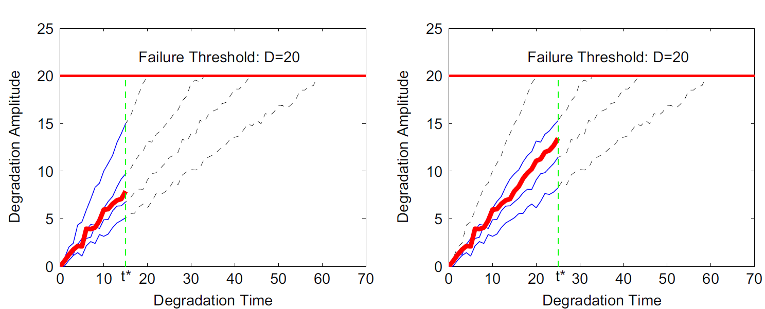
To address this challenge, we adopt the time-varying regression framework used in Fang, Zhou and Gebraeel (2015). The idea of the time-varying regression is that systems whose TTF are shorter than the current observation time (of the fielded system) are excluded from the training dataset. Next, the degradation data of the chosen systems are truncated at the current observation time as illustrated in Figure 1. By doing this, we ensure that the truncated degradation tensors of the chosen systems and the real-time observed degradation tensors of the fielded system possess the same dimensionality.

Figure 1: Method of updating the model as time advances (Fang, Zhou and Gebraeel, 2015)

We summarize the process of predicting and updating the RUL of a fielded system as follows:

1. At each sampling time $t_{n}$, a new degradation image is observed from a fielded system. Systems whose TTF are longer than $t_{n}$ are chosen from the training dataset.

2. The image streams of the chosen systems are then truncated at time $t_{n}$ by keeping only the images observed at times $\{t_{1},t_{2},\ldots,t_{n}\}$. The truncated image streams constitutes a new “training dataset”, hereafter referred to as truncated training dataset.

3. A dimensionality reduction technique, such as MPCA, is applied to the truncated training dataset to obtain a low-dimensional tensor subspace of the truncated training dataset. Tensors in the truncated training dataset are then projected to the tensor subspace and their low-dimensional approximations are estimated.

4. The low-dimensional approximation tensors are used to fit the regression model in Equation (2), and the parameters are estimated via one of the methods described in Sections 3.1 and 3.2.

5. The image stream from the fielded system is projected onto the tensor subspace estimated in step (iii), and its low-dimensional approximation is also estimated. Next, the approximated tensor is input into the regression model estimated in step (iv), and the TTF is predicted. The RUL is obtained by subtracting the current observation time from the predicted TTF.

Note that steps (i)-(iv) can be done offline. That is, given a training dataset, we can construct truncated training datasets with images observed at time $\{t_{1},t_{2}\}$, $\{t_{1},t_{2},t_{3}\}$, $\{t_{1},t_{2},t_{3},t_{4}\}$, $\ldots$, respectively. Regression models are then estimated based on all the possible truncated training datasets. Once a new image is observed at say time $t_{n}$, the appropriate regression model with images $\{t_{1},\ldots,t_{n}\}$ is chosen, and the RUL of the fielded system is estimated in step (v). This approach enables real-time RUL predictions.

5 Simulation study

In this section, we validate the effectiveness of our methodology with the two types of decomposition approaches using simulated degradation image streams. We assume the underlying physical degradation follows a heat transfer process based on which simulated degradation image streams are generated.

5.1 Data generation

Suppose for system $i$, the degradation image stream, denoted by $\mathcal{S}_{i}(x,y,t)$, $i=1,\ldots,1000$, is generated from the following heat transfer process: $\frac{\partial\mathcal{S}_{i}(x,y,t)}{\partial t}=\alpha_{i}(\frac{\partial^{2}\mathcal{S}_{i}}{\partial x^{2}}+\frac{\partial^{2}\mathcal{S}_{i}}{\partial y^{2}})$, where $(x,y);0\leq x,y\leq 0.05$ represents the location of each image pixel, $\alpha_{i}$ is the thermal diffusivity coefficient for system $i$ and is randomly generated from $uniform(0.5\times 10^{-5},1.5\times 10^{-5})$ and $t$ is the time frame. The initial and boundary conditions are set such that $\mathcal{S}|_{t=1}=0$ and $\mathcal{S}|_{x=0}=\mathcal{S}|_{x=0.05}=\mathcal{S}|_{y=0}=\mathcal{S}|_{y=0.05}=1$. At each time $t$, the image is recorded at locations $x=\frac{j}{n+1},y=\frac{k}{n+1},j,k=1,\ldots,n$, resulting in an $n\times n$ matrix. Here we set $n=21$ and $t=1,\ldots,10$, which leads to $10$ images of size $21\times 21$ for each system represented by a $21\times 21\times 10$ tensor. Finally, i.i.d noises $\varepsilon\sim N(0,0.01)$ are added to each pixel. Example degradation images observed at time $t=2,4,6,8,10$ from a simulated system are shown in Figure 2, in which (a) and (b) show images without and with noise, respectively.

(a) Without noise

(b) With noise

Figure 2: Simulated degradation images based on heat transfer process.

To simulate the TTF of each system two sets of coefficient tensors are used. The first set, denoted by $\mathcal{B}_{C}$, is simulated in the form of basis matrices with rank $2$ used in CP decomposition. Specifically, three matrices, i.e., $\boldsymbol{B}_{C,1}\in\mathbb{R}^{21\times 2},\boldsymbol{B}_{C,2}\in\mathbb{R}^{21\times 2},\boldsymbol{B}_{C,3}\in\mathbb{R}^{10\times 2}$ are generated. To induce sparsity, we randomly set half of elements of each matrix to be $0$. The values of the remaining $50\%$ elements are randomly generated from a uniform distribution $unif(-1,1)$. The TTF, denoted by $y_{C,i}$, is generated by using $y_{C,i}=\langle vec(\mathcal{B}_{C}),vec(\mathcal{S}_{i})\rangle+\sigma\epsilon_{i}$, where $vec({\mathcal{B}_{C}})=(\boldsymbol{B}_{C,3}\odot\boldsymbol{B}_{C,2}\odot\boldsymbol{B}_{C,1})\boldsymbol{1}_{2}$, $\epsilon_{i}$ follows a standard smallest extreme value distribution $\text{SEV}(0,1)$ and $\sigma$ is $5\%$ times the standard deviation of the location parameter, i.e., $\langle vec(\mathcal{B}_{C}),vec(\mathcal{S}_{i})\rangle$.

The second set, denoted by $\mathcal{B}_{T}$, is simulated in the form of core and factor matrices with rank $(2,1,2)$ used in Tucker decomposition. Specifically, a core tensor $\mathcal{G}_{T}\in\mathbb{R}^{2\times 1\times 2}$ and three factor matrices $\boldsymbol{B}_{T,1}\in\mathbb{R}^{21\times 2},\boldsymbol{B}_{T,2}\in\mathbb{R}^{21\times 1},\boldsymbol{B}_{T,3}\in\mathbb{R}^{10\times 2}$ are generated. All the elements of the core tensor $\mathcal{G}_{T}$ are set to $1$. Furthermore, half of elements of matrices $\boldsymbol{B}_{T,1},\boldsymbol{B}_{T,2},\boldsymbol{B}_{T,3}$ are randomly set to $0$ and the remaining elements are randomly generated from $unif(-1,1)$. The TTF, $y_{T,i}$, is generated via $y_{T,i}=\langle vec(\mathcal{B}_{T}),vec(\mathcal{S}_{i})\rangle+\sigma\epsilon_{i}$, where $vec({\mathcal{B}_{T}})=\mathcal{G}_{T}\times_{1}\boldsymbol{B}_{T,1}\times_{2}\boldsymbol{B}_{T,2}\times_{3}\boldsymbol{B}_{T,3}$, $\epsilon_{i}$ follows a standard smallest extreme value distribution $\text{SEV}(0,1)$ and $\sigma$ is $5\%$ times the standard deviation of the location parameter, i.e., $\langle vec(\mathcal{B}_{T}),vec(\mathcal{S}_{i})\rangle$.

In the following two subsections, we use the simulated degradation data to validate the proposed methodology. We first study the performance of the BIC criterion and our heuristic rank selection method in identifying the correct LLS distribution (i.e., SEV) as well as the right rank. Then, the prediction capability of our prognostic model is evaluated at different life percentiles of simulated systems. We randomly select $500$ of the simulated systems for training and the remaining $500$ systems for test.

5.2 Model and rank selection

We first apply CP-based tensor regression in Equation (5) to the training dataset, $\{y_{C,i},\mathcal{S}_{i}\}_{i=1}^{500}$, and use Algorithm 1 to estimate the model parameters for different ranks and for four LLS distributions, namely, normal, SEV, lognormal and Weibull. The BIC value is then computed for each distribution and rank combination as discussed in Section 3.1. As pointed out earlier, the block relaxation method in Algorithm 1 only guarantees a local optimum and hence, we shall run the algorithm 10 times using randomized initializations and record the smallest BIC. The BIC values for all combinations are reported in Table 1. From Table 1, it can be seen that the smallest BIC value is -1535.3, which belongs to SEV distribution with rank $R=2$. This coincides with the rank and the distribution we used to generate the data.

Table 1: BIC values for CP-based tensor regression.

Rank	R=1	R=2	R=3	R=4	R=5	R=6	R=7
SEV	620.5	-1535.3	-1383.4	-1232.7	-1122.9	-1014.4	-805.9
Normal	550.0	-1422.6	-1273.6	-1153.2	-1064.7	-1013.2	-1114.0
Weibull	618.1	-643.6	-472.6	-301.9	-180.5	-103.5	-54.0
Lognormal	610.5	-336.3	-187.7	-75.5	9.6	67.4	74.3

Similarly, the Tucker-based tensor regression model in Equation (12) is applied to the training dataset, $\{y_{T,i},\mathcal{S}_{i}\}_{i=1}^{500}$ and Algorithm 2 (see Section 3.2) is used to estimate the parameters. A total of $27$ different rank combinations are tested under four distributions, normal, SEV, lognormal and Weibull. Again, for each distribution-rank combination, Algorithm 2 is run with $10$ randomized initializations, and the smallest BIC value is reported in Table 2 .

Table 2: BIC values for Tucker-based tensor regression.

Rank	(1,1,1)	(1,1,2)	(1,1,3)	(1,2,1)	(1,2,2)	(1,2,3)	(1,3,1)	(1,3,2)	(1,3,3)
SEV	-163.3	-113.2	-75.8	-44.8	-59.0	-15.7	61.0	52.6	29.6
Normal	-199.0	-149.3	-112.0	-81.0	-82.8	-39.3	24.8	28.9	15.5
Weibull	-73.9	-24.4	13.0	44.1	35.9	79.2	149.6	147.4	133.5
Lognormal	-83.7	-33.9	3.4	34.4	28.6	71.6	140.0	140.2	141.9
Rank	(2,1,1)	(2,1,2)	(2,1,3)	(2,2,1)	(2,2,2)	(2,2,3)	(2,3,1)	(2,3,2)	(2,3,3)
SEV	-44.8	-1313.5	-1269.8	-16.1	-1212.7	-1202.9	95.4	-1115.0	-1106.5
Normal	-80.9	-1259.1	-1215.6	-22.9	-1149.7	-1130.8	89.3	-1048.6	-1028.2
Weibull	44.1	-733.8	-690.2	66.1	-633.2	-607.1	178.1	-543.5	-508.1
Lognormal	34.4	-497.8	-454.3	85.2-	-402.7	-394.4	197.2	-306.2	-292.6
Rank	(3,1,1)	(3,1,2)	(3,1,3)	(3,2,1)	(3,2,2)	(3,2,3)	(3,3,1)	(3,3,2)	(3,3,3)
SEV	60.7	-1201.8	-1224.9	95.5	-1156.4	-1164.0	113.0	-1071.4	-1074.4
Normal	24.9	-1147.2	-1153.2	88.8	-1093.2	-1082.6	129.4	-1009.0	-999.2
Weibull	149.7	-621.9	-613.1	177.8	-572.3	-539.2	205.6	-488.5	-468.2
Lognormal	139.9	-385.9	-391.0	197.5	-337.9	-331.4	238.5	-252.0	-262.3

Table 2 indicates that the smallest BIC value (-1313.5) is associated with the SEV distribution with rank $R=(2,1,2)$, which again matches the rank and the distribution that was used to generate the data. Therefore, we can conclude that the BIC criterion is effective in selecting an appropriate distribution as well as the correct rank of the tensors in the LLS regression. In Table 3, we also report the results of the heuristic rank selection method for Tucker. It can be seen from Table 3 that the heuristic rank selection method selects rank $R=(1,1,1)$ under normal and lognormal distributions, while selects rank $R=(2,2,2)$ under SEV distribution and $R=(1,2,2)$ under Weibull distribution. The smallest BIC values (-1212.3) is achieved under SEV distribution with rank $R=(2,2,2)$, which is close to the actual rank.

Table 3: Distribution and rank selection results by using heuristic rank selection method.

LLS Distribution	Rank	BIC
SEV	(2,2,2)	-1212.3
Normal	(1,1,1)	-199.0
Weibull	(1,2,2)	36.1
Lognormal	(1,1,1)	-83.7

5.3 RUL prediction results

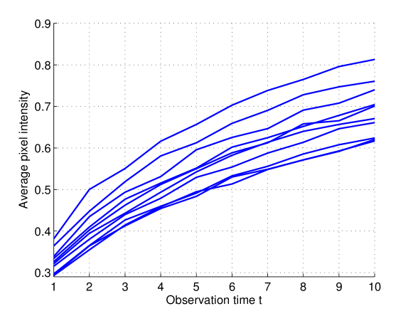
We evaluate the prediction accuracy of our prognostic model and compare its performance to a benchmark that uses functional principal components analysis (FPCA) to model the overall image intensity, which we designate as “FPCA”. For the benchmark, we first transform the degradation image stream of each system into a time-series signal by taking the average intensity of each observed image. A sample of transformed time-series degradation signals is shown in Figure 3. Next, FPCA is applied to the time-series signals to extract features. FPCA is a popular functional data analysis technique that identifies the important sources of patterns and variations among functional data (time-series signals in our case)(Ramsay and Silverman, 2005). The time-series signals are projected to a low-dimensional feature space spanned by the eigen-functions of the signals’ covariance function and provides fused features called FPC-scores. Finally, FPC-scores are regressed against the TTF by using LLS regression under SEV distribution. More details about this FPCA prognostic model can be found in (Fang, Zhou and Gebraeel, 2015).

Figure 3: A sample of time-series-based degradation signals.

The CP-based tensor regression model with rank $R=2$ under SEV distribution is applied to the training dataset to estimate the model. Next, the trained model is used to predict the TTFs of the test dataset using their degradation-based image observations. Prediction errors are calculated using the following expression:

$$\text{Prediction Error}=\frac{|\text{Estimated Lifetime-Real Lifetime}|}{\text{Real Lifetime}}$$ (19)

Two Tucker-based tensor regression models, one with rank $R=(2,1,2)$ selected by BIC and another with rank $R=(2,2,2)$ selected by heuristic rank selection method, are applied to the data under SEV distribution. The prediction errors of CP-based and Tucker-based tensor regression are reported in Figure 4 and 5, respectively.

Figure 4: Prediction errors of CP-based regression under SEV distribution.

Figure 5: Prediction errors of Tucker-based regression under SEV distribution.

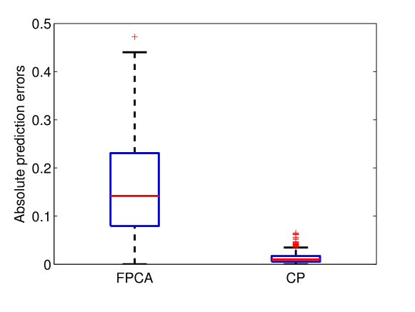
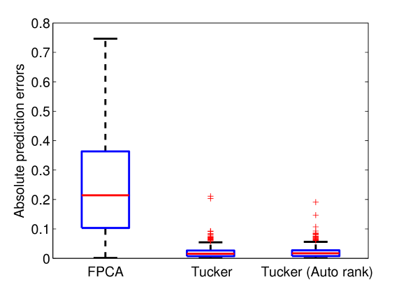
Figure 4 shows that the accuracy of the CP-based model is significantly better than the FPCA benchmark, where the mean prediction error is $15\%$ and $1\%$ for FPCA and our CP-based tensor regression, respectively. The variance of the prediction errors for FPCA is also much larger than that of CP-based tensor regression. Similar findings can be seen in Figure 5, where the mean prediction error of FPCA is 20%, and it is around 1% for Tucker-based tensor regression. The variance of the prediction errors for Tucker-based tensor regression is again much smaller than that of FPCA. The performance of the FPCA benchmark relative to our methodology highlights the importance of accounting for the spatial-temporal structure of image streams. The transformation of image streams to time-series signals ignores the spatial structure of images resulting in significant loss of information, and thus, compromising the prediction accuracy.

Figure 5 highlights the insignificant difference in prediction accuracy of the two proposed rank selection methods, BIC and heuristic rank selection (denoted “Tucker (Auto rank)” in the figure). This result further validates the effectiveness of our automatic rank selection method.

6 Case study: Degradation image streams from rotating machinery

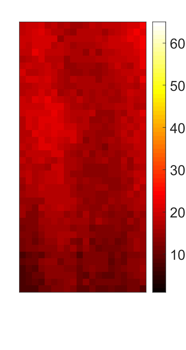
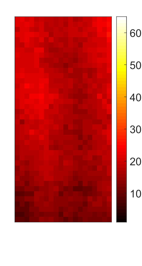
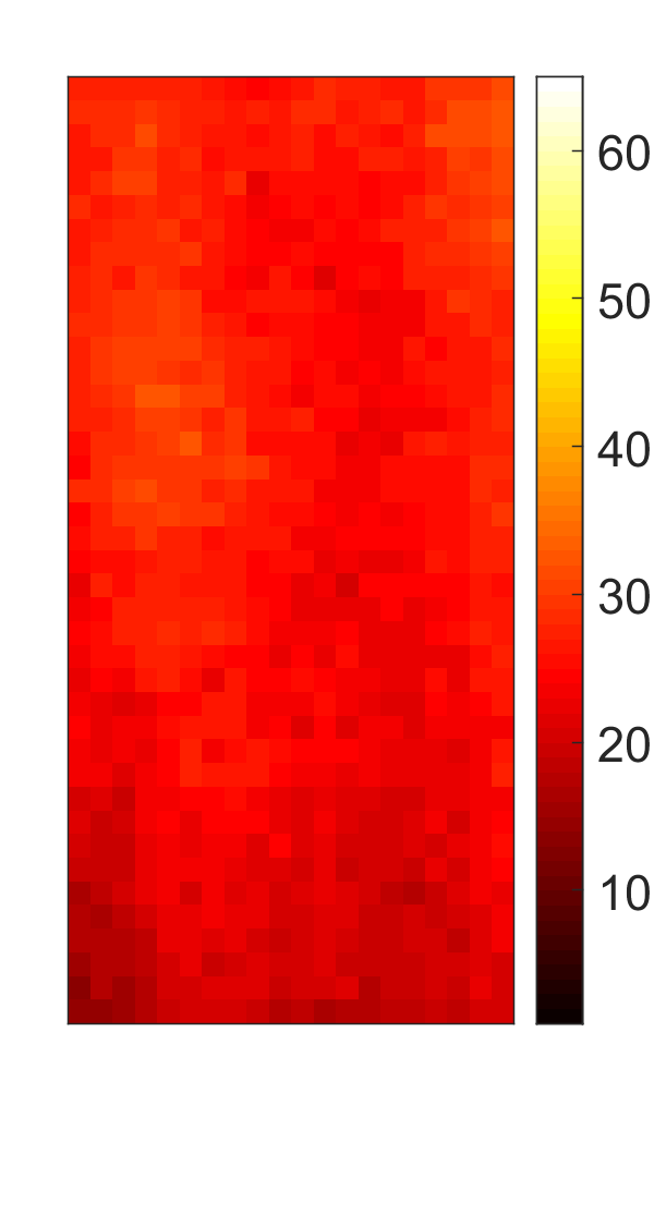
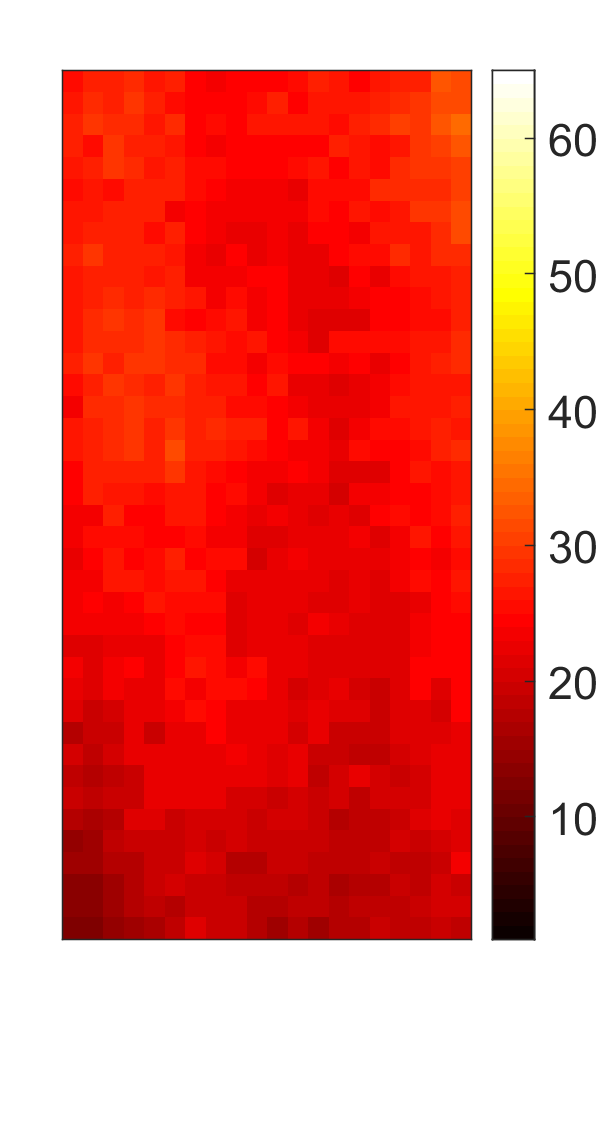
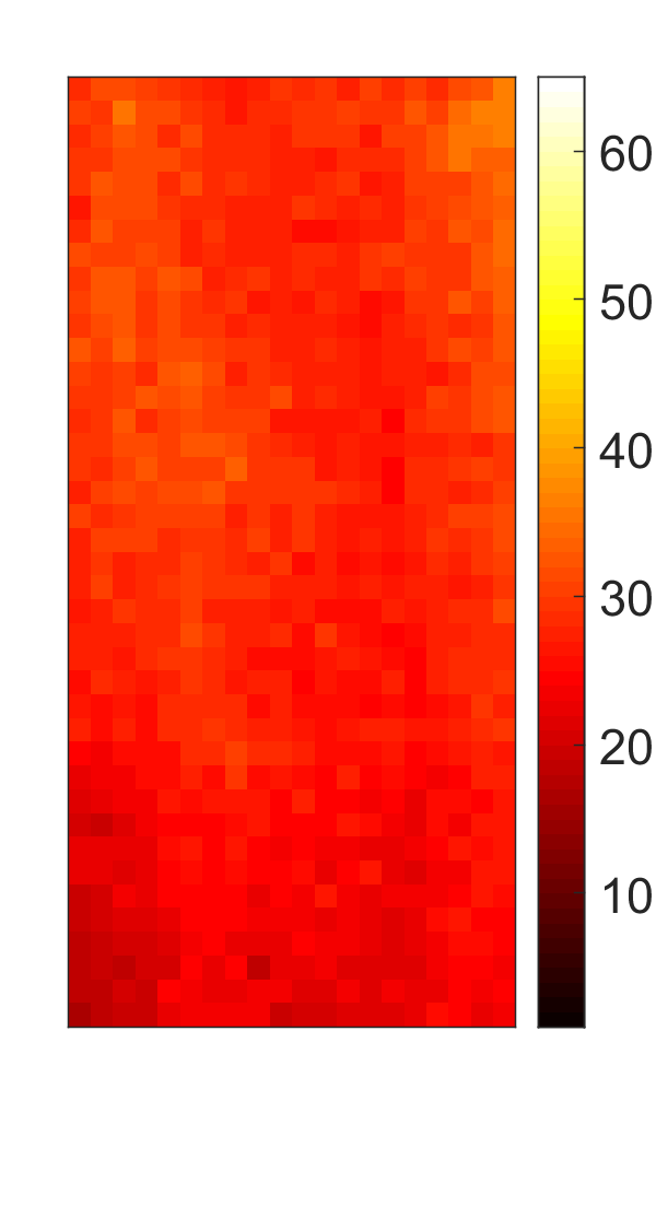
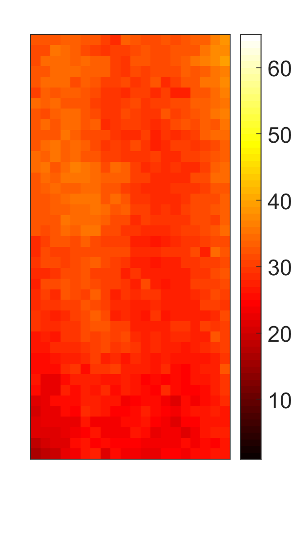
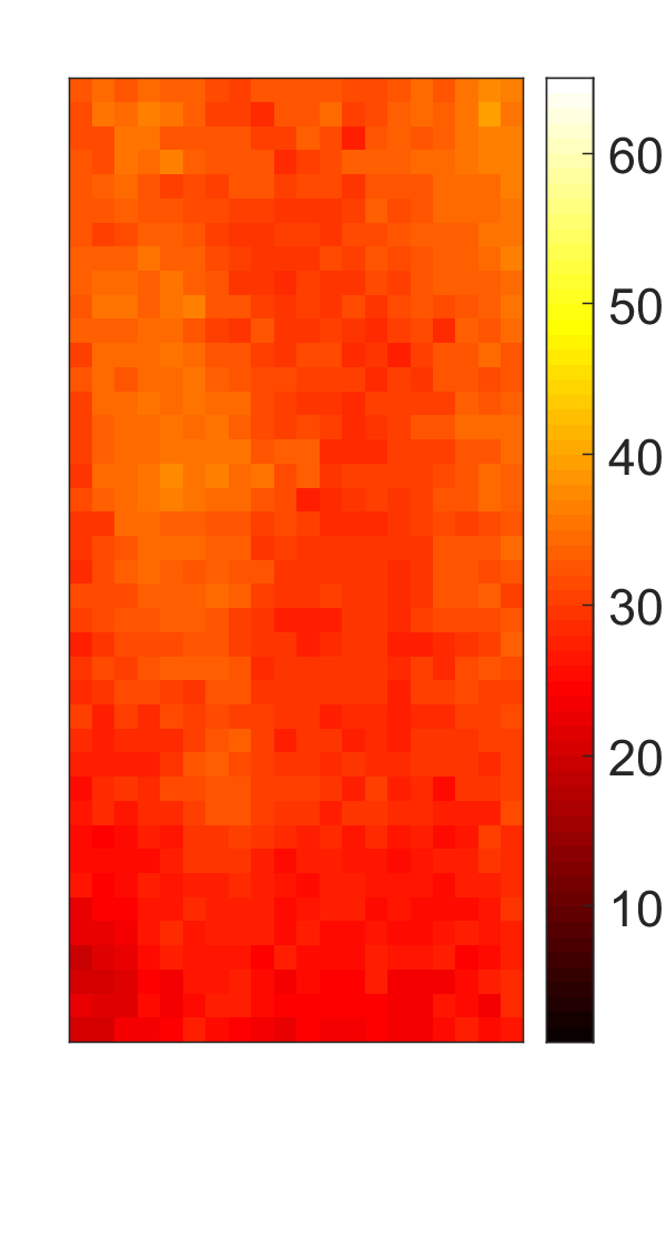
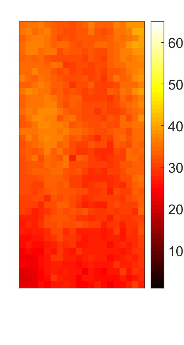
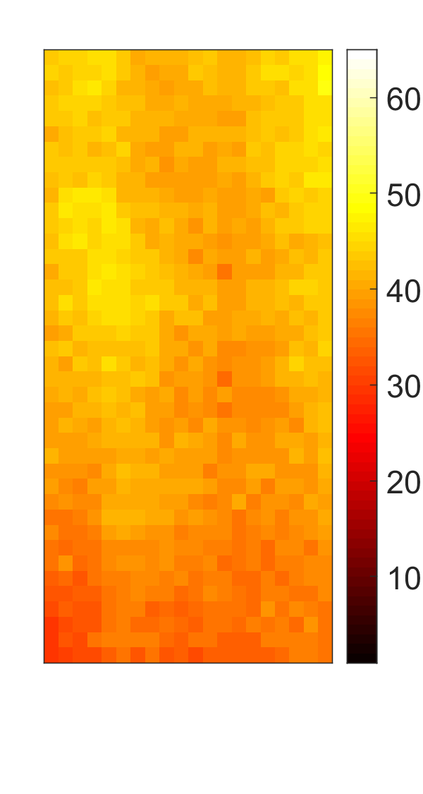
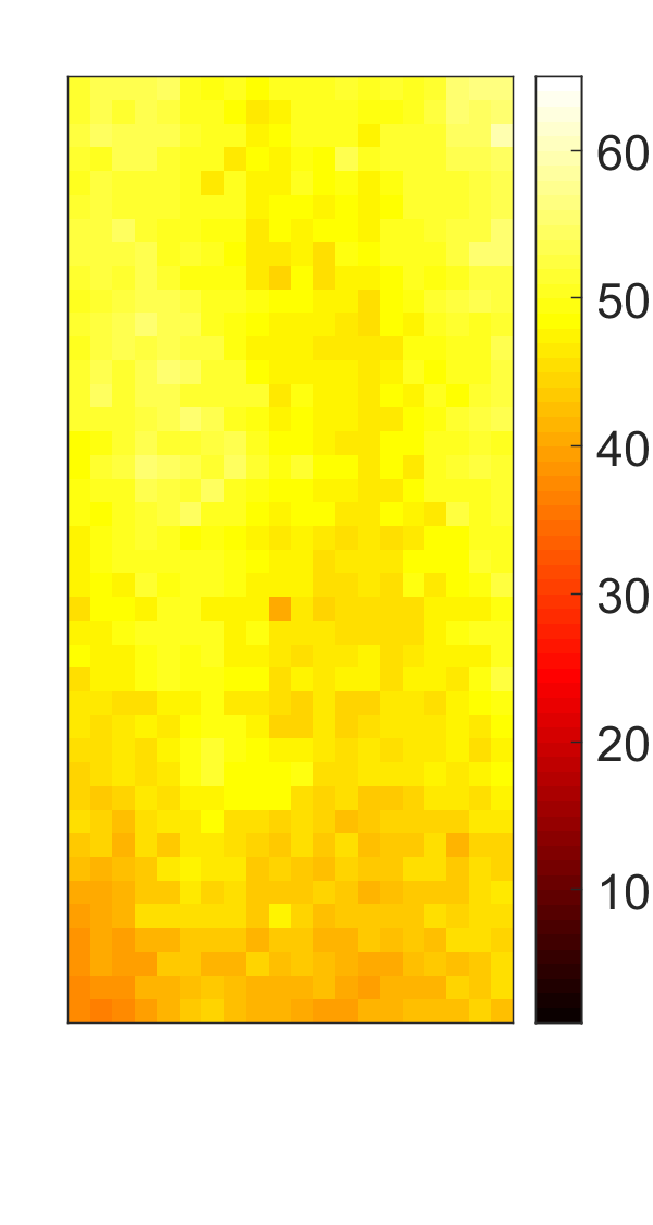
In this section, we validate the effectiveness of our methodology using degradation image streams obtained from a rotating machinery. The experimental test bed, which was described in detail in Gebraeel, Elwany and Pan (2009), is designed to perform accelerated degradation tests on rolling element thrust bearings. The test bearings are run from a brand new state until failure. Vibration sensors are used to monitor the health of the rotating machinery. Failure is defined once the amplitude of defective vibration frequencies crosses a pre-specified threshold based on ISO standards for machine vibration. Meanwhile, infrared images that capture temperature signatures of the degraded component throughout the degradation test are acquired using an FLIR T300 infrared camera. Infrared images with $40\times 20$ pixels are stored every $10$ seconds. Four different experiments were run to failure. The resulting degradation-based image streams contained $375$, $611$, $827$ and $1,478$ images, respectively.

Due to the high cost of running degradation experiments, additional degradation image streams were generated by resampling from the original image database obtained from the four experiments discussed earlier. In total 284 image data streams were generated. As an illustration, a sequence of images obtained at different (ordered) time periods are shown in Figure 6.

(a) t=1

(b) t=2

(c) t=3

(d) t=4

(e) t=5

(f) t=6

(g) t=7

(h) t=8

(i) t=9

(j) t=10

Figure 6: An illustration of one infrared degradation image stream.

6.1 Model selection

In this section, we discuss how to select an appropriate LLS tensor regression model for our dataset. This is achieved by applying different LLS tensor regression candidate models to a training set consisting of multiple image data streams. The model with the smallest BIC is selected as the best candidate model.

To account for the variability in the length of the image streams (as illustrated earlier in Section 4), we generate multiple subsamples based on different TTFs. Specifically, we sort the TTFs in ascending order such that $TTF_{1}<TTF_{2}<\cdots<TTF_{n}$, where $n\leq 284$ is the number of unique TTFs (or equivalent the number of subsamples). Next, we define subsample $i$ as the systems whose TTFs are greater than or equal to $TTF_{i}$, for $i=1,\ldots,n$. For example, subsample $1$ includes all the $284$ image streams, and subsample $2$ includes all the image streams excluding the ones with the smallest TTF, and so forth. Third, each subsample is truncated by only keeping images observed on time domain $[0,TTF_{i}]$ epochs. By doing so, we ensure that all the image streams in a subsample have the same dimensionality. This is important when applying the LLS tensor regression model. After truncation, the following steps are applied to select the best candidate regression model:

• Step 1: Dimension reduction. MPCA is applied to each subsample $i$ (truncated image stream). The fraction-of-variance-explained, which is used to select the number of multilinear principal components (see Lu, Plataniotis and Venetsanopoulos (2008) for details), is set to be $0.95$. Using this criterion, a low-dimensional tensor is extracted from each image stream (or each system).

• Step 2: Fitting LLS model. The low-dimensional tensors extracted from Step 1 are regressed against TTFs using an LLS regression model. Similar to the Simulation study, we evaluate four types of distributions: normal, lognormal, SEV and Weibull. Tucker-based estimation method with heuristic rank selection is used for parameter estimation.

• Step 3: Comparing BIC values. BIC values are then computed for each of the four fitted models. The model with the smallest BIC is selected as the most appropriate one for the subsample.

• Step 4: Distribution selection. Steps 1, 2, and 3 are applied to all the subsamples. The distribution with the highest selected frequency is considered as the best candidate distribution.

After applying the aforementioned selection procedures to all the subsamples, we summarize the percentage of times each distribution was selected. Table 4 summarizes these results and shows that the Weibull distribution was selected on average $74.4\%$ while the lognormal was selected $25.6\%$ of the time. We expect to have some overlap in the models that have been selected because for specific parameter values, different distributions may exhibit reasonable fits for the same data sets. In our case, it is clear that the Weibull distribution dominates most of the selections and will therefore be considered as the suitable distribution for this data set.

Table 4: Distribution selection results.

LLS Distribution	Normal	Lognormal	SEV	Weibull
Selection (%)	$0\%$	$25.6\%$	$0\%$	$74.4\%$

6.2 Performance Evaluation

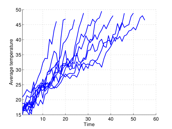
The Weibull tensor regression model is chosen for evaluating the accuracy of predicting lifetime. Similar to the simulation study in Section 5, we compare the performance of our methods with the FPCA approach, denoted by “FPCA”. Time-series degradation signals corresponding to the infrared images of the experimental test bed were obtained in a similar manner to what was discussed in Section 5. Figure 7 shows a sample of these transformed time-series signals.

Figure 7: A sample of transformed time-series signals.

The accuracy and precision of the predictions made by the proposed model as well as the FPCA model are evaluated using a leave-one-out cross-validation study. For each validation, $283$ systems are used for training and the remaining one system is used for testing. The RULs of the test system are predicted at each time epoch. The time-varying regression framework presented in Section 4 is used to enable the integration of newly observed image data (from the test data). The prediction errors are computed using Equation (19). We report the mean and variance of the absolute prediction errors in Figure 8 where $10\%$ represents prediction errors evaluated at life percentiles in the interval of $(5\%,15\%]$, $20\%$ for the interval of $(15\%,25\%]$, etc.

(a) mean

(b) variance

Figure 8: The mean and variance of the absolute prediction errors.

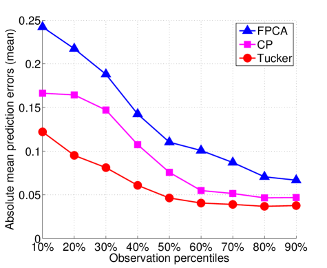
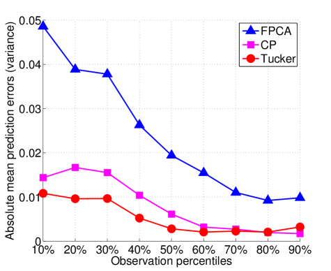
Figure 8 indicates that all the three methodologies have smaller prediction errors at higher observation percentiles. This is because at higher observation percentiles more degradation-based image data has been observed, which provide more information about the underlying physical degradation process. This results in better prediction accuracy. Figure 8 also shows that the proposed CP-based and Tucker-based regression models outperform the FPCA model in terms of mean and variance of the absolute prediction errors. For example, at the $50^{th}$ percentile, the mean (variance) of the absolute prediction errors for FPCA, CP-based and Tucker-based models are $0.12(0.02)$, $0.07(0.006)$ and $0.05(0.003)$, respectively. A similar pattern can also be seen at the remaining prediction percentiles. As mentioned earlier, one explanation for this phenomenon is that by averaging the pixel intensities we break the spatio-temporal structure of the image, which is clearly an important aspect that needs to be considered when modeling how images evolve spatially and temporally–a key aspect that is addressed by our modeling framework.

Figure 8 also shows that Tucker-based regression performs better than CP-based. The mean and variance for the Tucker-based model are consistently lower than those of the CP-based regression model. This difference may be attributed to the fact that the Tucker-based model allows the tensor to have a different rank for each of the three orders (directions). This enhances the flexibility of the regression model. In contrast, the CP-based model requires the rank on each direction to be equal, which may have an impact on the model’s flexibility.

7 Conclusions

Degradation tensors such image streams and profiles often contain rich information about the physical degradation process and can be utilized for prognostics and predicting the RUL of functioning systems. However, the analysis of degradation tensors is challenging due to their high-dimensionality and complex spatial-temporal structure. In this paper, we proposed a penalized (log)-location-scale regression model that can utilize high dimensional tensors to predict the RUL of systems. Our method first reduces the dimensionality of tensor covariates by projecting them onto a low-dimensional tensor subspace that preserves the useful information of the covariates. Next, the projected low-dimensional covariate tensors are regressed against TTFs via an LLS regression model. In order to further reduce the number of parameters, the coefficient tensor is decomposed by utilizing two tensor decompositions, CP and Tucker. The CP decomposition decomposes the coefficient tensor as a product of low-dimensional basis matrices, and Tucker decomposition expresses it as a product of a low-dimensional core tensor and factor matrices. Instead of estimating the coefficient tensor, we only estimate its corresponding core tensors and factor/basis matrices. By doing so, the number of parameters to be estimated is dramatically reduced. Two numerical block relaxation algorithms with global convergence property were developed for the model estimation. The block relaxation algorithms iteratively estimate only one block of parameters (i.e., one factor/basis matrix or core tensor) at each time while keeping other blocks fixed until convergences.

We evaluated the performance of our proposed methodology through numerical studies. The results indicated that our methodology outperformed the benchmark in terms of both prediction accuracy and precision. For example, the mean prediction error for CP-based tensor regression model is 1%, while it is 15% for the benchmark. In addition, we showed that the absolute mean prediction error for Tucker-based regression model and the benchmark are 1% and 20%, respectively. We also validated the effectiveness of our proposed tensor regression model using a case study on degradation modeling of bearings in a rotating machinery. The results indicated that both CP-based and Tucker-based models outperformed the benchmark in terms of prediction accuracy as well as precision at all life percentiles. As an example, the mean (variance) of prediction errors at the 50th observation percentile are 12% (2%), 7% (0.6%) and 5% (0.3%) for FPCA, CP-based model and Tucker-based model, respectively. The results also indicated that Tucker-based model achieved better prediction accuracy than the CP-based model. This is reasonable since Tucker-based model is more flexible as it allows different modes to have different ranks, while the CP-based model requires all the modes have the same rank. The model developed in this paper only works on a single computer. Development of a tensor-based prognostics model that can run on a distributed computing system is an important topic for future research.

Appendix A Proof of Proposition 1

The proof follows the proof of Lemma 1 in Li, Zhou and Li (2013). Specifically, the mode-$d$ matricization of tensor $\mathcal{S}_{i}$ and $\tilde{\mathcal{B}}$ can be expressed as (Li, Zhou and Li, 2013):

$$\begin{split}\boldsymbol{S}_{i(d)}=\boldsymbol{U}_{d}\tilde{\boldsymbol{S}}_{i(d)}\left(\boldsymbol{U}_{D}\otimes\cdots\otimes\boldsymbol{U}_{d+1}\otimes\boldsymbol{U}_{d-1}\otimes\cdots\otimes\boldsymbol{U}_{1}\right)^{\top},\\ \tilde{\boldsymbol{B}}_{(d)}=\boldsymbol{U}_{d}^{\top}{\boldsymbol{B}}_{(d)}\left(\boldsymbol{U}_{D}\otimes\cdots\otimes\boldsymbol{U}_{d+1}\otimes\boldsymbol{U}_{d-1}\otimes\cdots\otimes\boldsymbol{U}_{1}\right).\end{split}$$

Then, we have the following:

$$\begin{split}&\langle\mathcal{B},\mathcal{S}_{i}\rangle\\ &=\langle\boldsymbol{B}_{(d)},\boldsymbol{S}_{i(d)}\rangle\\ &=\langle{\boldsymbol{B}}_{(d)},\boldsymbol{U}_{d}\tilde{\boldsymbol{S}}_{i(d)}\left(\boldsymbol{U}_{D}\otimes\cdots\otimes\boldsymbol{U}_{d+1}\otimes\boldsymbol{U}_{d-1}\otimes\cdots\otimes\boldsymbol{U}_{1}\right)^{\top}\rangle\\ &=\langle\boldsymbol{U}_{d}^{\top}{\boldsymbol{B}}_{(d)}\left(\boldsymbol{U}_{D}\otimes\cdots\otimes\boldsymbol{U}_{d+1}\otimes\boldsymbol{U}_{d-1}\otimes\cdots\otimes\boldsymbol{U}_{1}\right),\tilde{\boldsymbol{S}}_{i(d)}\rangle\\ &=\langle\tilde{\boldsymbol{B}}_{(d)},\tilde{\boldsymbol{S}}_{i(d)}\rangle\\ &=\langle\tilde{\mathcal{B}},\tilde{\mathcal{S}}_{i}\rangle\end{split}$$

Appendix B Optimization Algorithm for Problem (3)

The pseudocode of the algorithm is shown in Table 5 (Lu, Plataniotis and Venetsanopoulos, 2008)

Input: A set of tensor samples $\left\{\mathcal{S}_{i}\in R^{I_{1}\times\cdots\times I_{D}}\right\}_{i=1}^{N}$

Output: Low-dimensional representations $\left\{\mathcal{\tilde{S}}_{i}\in R^{P_{1}\times\cdots\times P_{D}}\right\}_{i=1}^{N}$of the input tensor samples with maximum variation captured

Algorithm:

Step 1 (Preprocessing): Center the input samples as $\left\{\mathcal{X}_{i}=\mathcal{S}_{i}-\bar{\mathcal{S}}\right\}_{i=1}^{N}$ , where $\bar{\mathcal{S}}=\frac{1}{N}\sum_{i=1}^{N}\mathcal{S}_{i}$ is the sample mean Step 2 (Initialization): Calculate the eigen-decomposition of $\boldsymbol{\Phi}_{(d)}^{*}=\sum_{i=1}^{N}\boldsymbol{X}_{i(d)}\boldsymbol{X}_{i(d)}^{\top}$ and set $\boldsymbol{U}_{d}$ to consist of the eigenvectors corresponding to the most significant $P_{d}$ eigenvalues, for $d=1,\ldots D$ Step 3 (Local optimization): (i) Calculate $\left\{\tilde{\mathcal{X}_{i}}=\mathcal{X}_{i}\times_{1}\boldsymbol{U}_{1}^{\top}\times_{2}\boldsymbol{U}_{2}^{\top}\times\cdots\times_{D}\boldsymbol{U}_{D}^{\top}\right\}_{i=1}^{N}$ (ii) Calculate $\Psi_{0}=\sum_{i=1}^{N}||\tilde{\mathcal{X}_{i}}||_{F}^{2}$ (the mean of $\left\{\tilde{\mathcal{X}_{i}}\right\}_{i=1}^{N}$ is all zero since $\left\{\mathcal{X}_{i}\right\}_{i=1}^{N}$is centered. (iii) For $k=1:K$ – For $d=1:D$ Calculate the eigen-decomposition of $\boldsymbol{\Phi}_{(d)}$ and set $\boldsymbol{U}_{d}$ to consist of the eigenvectors corresponding to the most significant $P_{d}$ eigenvalues, for $d=1,\ldots D$, where $\boldsymbol{\Phi}_{(d)}=\sum_{i=1}^{N}\left(\boldsymbol{S}_{i(d)}-\bar{\boldsymbol{S}}_{(d)}\right)\cdot\boldsymbol{A}_{d}\cdot\boldsymbol{A}_{d}^{\top}\cdot\left(\boldsymbol{S}_{i(d)}-\bar{\boldsymbol{S}}_{(d)}\right)^{\top}$ and $\boldsymbol{A}_{d}=\left(\boldsymbol{U}_{d+1}\otimes\boldsymbol{U}_{d+2}\otimes\cdots\otimes\boldsymbol{U}_{D}\otimes\boldsymbol{U}_{1}\otimes\boldsymbol{U}_{2}\otimes\cdots\otimes\boldsymbol{U}_{d-1}\right)$ – Calculate $\left\{\tilde{\mathcal{S}_{i}}\right\}_{i=1}^{N}$ and $\Psi_{k}$ – If $\Psi_{k}-\Psi_{k}<\eta$, break and go to Step 4. Step 4 (Projection): The feature tensor after projection is obtained as $\left\{\tilde{\mathcal{S}_{i}}=\mathcal{S}_{i}\times_{1}\boldsymbol{U}_{1}^{\top}\times_{2}\boldsymbol{U}_{2}^{\top}\times\cdots\times_{D}\boldsymbol{U}_{D}^{\top}\right\}_{i=1}^{N}$

Table 5: Pseudocode implementation of the MPCA algorithm (Lu, Plataniotis and Venetsanopoulos, 2008).

Appendix C Proof of Proposition 2

Based on the CP decomposition, tensor $\mathcal{B}$ has the following properties (Li, Zhou and Li, 2013):

$\begin{array}[]{cc}&vec({\mathcal{B}})=(\boldsymbol{B}_{D}\odot\cdots\odot\boldsymbol{B}_{1})\boldsymbol{1}_{R},\\ &\boldsymbol{B}_{(d)}=\boldsymbol{B}_{d}(\boldsymbol{B}_{D}\odot\cdots\odot\boldsymbol{B}_{d+1}\odot\boldsymbol{B}_{d-1}\odot\cdots\odot\boldsymbol{B}_{1})^{\top}\end{array}$

Recall the optimization problem is

$$\operatorname*{arg\,max}_{\boldsymbol{\theta}}\left\{-N\log\sigma+\sum_{i=1}^{N}\log f\left(\frac{y_{i}-\alpha-\left\langle(\tilde{\boldsymbol{B}}_{D}\odot\cdots\odot\tilde{\boldsymbol{B}}_{1})\boldsymbol{1}_{R},{vec}(\tilde{\mathcal{S}}_{i})\right\rangle}{\sigma}\right)-\sum_{d=1}^{D}r\left(\tilde{\boldsymbol{B}}_{d}\right)\right\}$$

Given $\left\{\tilde{\boldsymbol{B}}_{1},\ldots,\tilde{\boldsymbol{B}}_{d-1},\tilde{\boldsymbol{B}}_{d+1},\ldots,\tilde{\boldsymbol{B}}_{D}\right\}$,the inner product in the optimization is

$\begin{array}[]{cl}&\langle(\boldsymbol{B}_{D}\odot\cdots\odot\boldsymbol{B}_{1})\boldsymbol{1}_{R},{vec}(\tilde{\mathcal{S}}_{i})\rangle\\ =&\langle{vec}(\tilde{\mathcal{B}}),{vec}(\tilde{\mathcal{S}}_{i})\rangle\\ =&\langle\tilde{\mathcal{B}},\tilde{\mathcal{S}}_{i}\rangle\\ =&\langle\tilde{\boldsymbol{B}}_{(d)},\tilde{\boldsymbol{S}}_{i(d)}\rangle\\ =&\langle\boldsymbol{B}_{d}(\boldsymbol{B}_{D}\odot\cdots\odot\boldsymbol{B}_{d+1}\odot\boldsymbol{B}_{d-1}\odot\cdots\odot\boldsymbol{B}_{1})^{\top},\tilde{\boldsymbol{S}}_{i(d)}\rangle\\ =&\langle\boldsymbol{B}_{d},\tilde{\boldsymbol{S}}_{i(d)}(\boldsymbol{B}_{D}\odot\cdots\odot\boldsymbol{B}_{d+1}\odot\boldsymbol{B}_{d-1}\odot\cdots\odot\boldsymbol{B}_{1})\rangle\\ =&\langle\boldsymbol{B}_{d},\boldsymbol{X}_{d,i}\rangle\end{array}$

where $\boldsymbol{X}_{d,i}=\tilde{\boldsymbol{S}}_{i(d)}(\boldsymbol{B}_{D}\odot\cdots\odot\boldsymbol{B}_{d+1}\odot\boldsymbol{B}_{d-1}\odot\cdots\odot\boldsymbol{B}_{1})$. Therefore, the optimization problem can be re-expressed as

$$\operatorname*{arg\,max}_{\boldsymbol{\theta}}\left\{-N\log\sigma+\sum_{i=1}^{N}\log f\left(\frac{y_{i}-\alpha-\langle\boldsymbol{B}_{d},\boldsymbol{X}_{d,i}\rangle}{\sigma}\right)-\sum_{d=1}^{D}r\left(\tilde{\boldsymbol{B}}_{d}\right)\right\}$$

Appendix D Invariant Property of Optimization Problem (8)

Recall optimization problem (8)

$$\operatorname*{arg\,max}_{\boldsymbol{\tilde{B}}_{d},\sigma,\alpha}\left\{-N\ln\sigma+\sum_{i=1}^{N}\ln f\left(\frac{y_{i}-\alpha-\left\langle\tilde{\boldsymbol{B}}_{d},\boldsymbol{X}_{d,i}\right\rangle}{\sigma}\right)-r(\frac{\tilde{\boldsymbol{B}}_{d}}{\sigma})\right\}$$

Consider the transformation $y_{i}^{\prime}=by_{i},\alpha^{\prime}=b\alpha,\tilde{\boldsymbol{B}}_{d}^{\prime}=b\tilde{\boldsymbol{B}_{d}},\sigma^{\prime}=b\sigma$ where $b>0$, we have

$\begin{array}[]{cl}&\operatorname*{arg\,max}_{\boldsymbol{\tilde{B}}_{d}^{\prime},\sigma^{\prime},\alpha^{\prime}}\left\{-N\ln\sigma^{\prime}+\sum_{i=1}^{N}\ln f\left(\frac{y_{i}^{\prime}-\alpha^{\prime}-\left\langle\tilde{\boldsymbol{B}}_{d}^{\prime},\boldsymbol{X}_{d,i}\right\rangle}{\sigma}\right)-r(\frac{\tilde{\boldsymbol{B}}_{d}^{\prime}}{\sigma^{\prime}})\right\}\\ \iff&\operatorname*{arg\,max}_{\boldsymbol{\tilde{B}}_{d},\sigma,\alpha}\left\{-N\ln\left(b\sigma\right)+\sum_{i=1}^{N}\ln f\left(\frac{by_{i}-b\alpha-\left\langle b\tilde{\boldsymbol{B}}_{d},\boldsymbol{X}_{d,i}\right\rangle}{b\sigma}\right)-r(\frac{b\tilde{\boldsymbol{B}}_{d}}{b\sigma})\right\}\\ \iff&\operatorname*{arg\,max}_{\boldsymbol{\tilde{B}}_{d},\sigma,\alpha}\left\{-N\ln\left(b\sigma\right)+\sum_{i=1}^{N}\ln f\left(\frac{by_{i}-b\alpha-b\left\langle\tilde{\boldsymbol{B}}_{d},\boldsymbol{X}_{d,i}\right\rangle}{b\sigma}\right)-r(\frac{b\tilde{\boldsymbol{B}}_{d}}{b\sigma})\right\}\\ \iff&\operatorname*{arg\,max}_{\boldsymbol{\tilde{B}}_{d},\sigma,\alpha}\left\{-N\ln b-N\ln\sigma+\sum_{i=1}^{N}\ln f\left(\frac{y_{i}-\alpha-\left\langle\tilde{\boldsymbol{B}}_{d},\boldsymbol{X}_{d,i}\right\rangle}{\sigma}\right)-r(\frac{\tilde{\boldsymbol{B}}_{d}}{\sigma})\right\}\\ \iff&\operatorname*{arg\,max}_{\boldsymbol{\tilde{B}}_{d},\sigma,\alpha}\left\{-N\ln\sigma+\sum_{i=1}^{N}\ln f\left(\frac{y_{i}-\alpha-\left\langle\tilde{\boldsymbol{B}}_{d},\boldsymbol{X}_{d,i}\right\rangle}{\sigma}\right)-r(\frac{\tilde{\boldsymbol{B}}_{d}}{\sigma})\right\}\end{array}$

Appendix E Proof of Proposition 3

Based on the Tucker decomposition, tensor $\mathcal{B}$ has the following properties (Li, Zhou and Li, 2013):

$\begin{array}[]{cc}&\boldsymbol{B}_{(d)}=\boldsymbol{B}_{d}\boldsymbol{G}_{(d)}(\boldsymbol{B}_{D}\otimes\cdots\otimes\boldsymbol{B}_{d+1}\otimes\boldsymbol{B}_{d-1}\otimes\cdots\otimes\boldsymbol{B}_{1})^{\top},\\ &vec({\mathcal{B}})=(\boldsymbol{B}_{D}\otimes\cdots\otimes\boldsymbol{B}_{1})vec(\mathcal{G}).\end{array}$

Recall the optimization problem is

$$\operatorname*{arg\,max}_{\boldsymbol{\theta}}\left\{-N\ln\sigma+\sum_{i=1}^{N}\ln f\left(\frac{y_{i}-\alpha-\left\langle\mathcal{\tilde{G}}\times_{1}\tilde{\boldsymbol{B}}_{1}\times_{2}\tilde{\boldsymbol{B}}_{2}\times_{3}\cdots\times_{D}\tilde{\boldsymbol{B}}_{D},\tilde{\mathcal{S}}_{i}\right\rangle}{\sigma}\right)\right.$$

$$\left.-r(\mathcal{\mathcal{\tilde{G}}})-\sum_{d=1}^{D}r\left(\tilde{\boldsymbol{B}}_{d}\right)\right\},$$

Given $\left\{\tilde{\boldsymbol{B}}_{1},\tilde{\boldsymbol{B}}_{2}\ldots,\tilde{\boldsymbol{B}}_{D}\right\}$, the inner product in the optimization can be expressed as

$\begin{array}[]{cl}&\langle\mathcal{\tilde{G}}\times_{1}\tilde{\boldsymbol{B}}_{1}\times_{2}\tilde{\boldsymbol{B}}_{2}\times_{3}\cdots\times_{D}\tilde{\boldsymbol{B}}_{D},\tilde{\mathcal{S}}_{i}\rangle\\ =&\langle\tilde{\mathcal{B}},\tilde{\mathcal{S}}_{i}\rangle\\ =&\langle vec(\tilde{\mathcal{B}}),vec(\tilde{\mathcal{S}}_{i})\rangle\\ =&\langle(\tilde{\boldsymbol{B}}_{D}\otimes\cdots\otimes\tilde{\boldsymbol{B}}_{1})vec(\mathcal{\mathcal{\mathcal{\tilde{G}}}}),vec(\tilde{\mathcal{S}}_{i})\rangle\\ =&\langle vec(\mathcal{\mathcal{\mathcal{\tilde{G}}}}),(\tilde{\boldsymbol{B}}_{D}\otimes\cdots\otimes\tilde{\boldsymbol{B}}_{1})^{\top}vec(\tilde{\mathcal{S}}_{i})\rangle\end{array}$

Therefore, the optimization problem can be re-expressed as

$$\operatorname*{arg\,max}_{\mathcal{\mathcal{\mathcal{\mathcal{\tilde{G}}}}}}\left\{-N\ln\sigma+\sum_{i=1}^{N}\ln f\left(\frac{y_{i}-\alpha-\left\langle vec(\mathcal{\mathcal{\mathcal{\mathcal{\tilde{G}}}}}),(\tilde{\boldsymbol{B}}_{D}\otimes\cdots\otimes\tilde{\boldsymbol{B}}_{1})^{\top}vec(\tilde{\mathcal{S}}_{i})\right\rangle}{\sigma}\right)-r(\mathcal{\mathcal{\mathcal{\mathcal{\tilde{G}}}}})\right\},$$

Appendix F Proof for Proposition 4

Recall the optimization problem is

$$\operatorname*{arg\,max}_{\boldsymbol{\theta}}\left\{-N\ln\sigma+\sum_{i=1}^{N}\ln f\left(\frac{y_{i}-\alpha-\left\langle\mathcal{\tilde{G}}\times_{1}\tilde{\boldsymbol{B}}_{1}\times_{2}\tilde{\boldsymbol{B}}_{2}\times_{3}\cdots\times_{D}\tilde{\boldsymbol{B}}_{D},\tilde{\mathcal{S}}_{i}\right\rangle}{\sigma}\right)\right.$$

$$\left.-r(\mathcal{\mathcal{\tilde{G}}})-\sum_{d=1}^{D}r\left(\tilde{\boldsymbol{B}}_{d}\right)\right\},$$

Given $\mathcal{\tilde{G}}$ and $\left\{\tilde{\boldsymbol{B}}_{1},\ldots,\tilde{\boldsymbol{B}}_{d-1},\tilde{\boldsymbol{B}}_{d+1},\ldots,\tilde{\boldsymbol{B}}_{D}\right\}$, the inner product in the optimization can be expressed as

$\begin{array}[]{ll}&\langle\mathcal{G}\times_{1}\boldsymbol{B}_{1}\times_{2}\boldsymbol{B}_{2}\times_{3}\cdots\times_{D}\boldsymbol{B}_{D},\tilde{\mathcal{S}}_{i}\rangle\\ =&\langle\tilde{\mathcal{B}},\tilde{\mathcal{S}}_{i}\rangle\\ =&\langle\tilde{\boldsymbol{B}}_{(d)},\tilde{\boldsymbol{S}}_{i(d)}\rangle\\ =&\langle\boldsymbol{B}_{d}\boldsymbol{G}_{(d)}(\boldsymbol{B}_{D}\otimes\cdots\otimes\boldsymbol{B}_{d+1}\otimes\boldsymbol{B}_{d-1}\otimes\cdots\otimes\boldsymbol{B}_{1})^{\top},\tilde{\boldsymbol{S}}_{i(d)}\rangle\\ =&\langle\boldsymbol{B}_{d},\tilde{\boldsymbol{S}}_{i(d)}(\boldsymbol{B}_{D}\otimes\cdots\otimes\boldsymbol{B}_{d+1}\otimes\boldsymbol{B}_{d-1}\otimes\cdots\otimes\boldsymbol{B}_{1})\boldsymbol{G}_{(d)}^{\top}\rangle\\ =&\langle\boldsymbol{B}_{d},\boldsymbol{X}_{d,i}\rangle\end{array}$

where $\boldsymbol{X}_{d,i}=\tilde{\boldsymbol{S}}_{i(d)}(\boldsymbol{B}_{D}\otimes\cdots\otimes\boldsymbol{B}_{d+1}\otimes\boldsymbol{B}_{d-1}\otimes\cdots\otimes\boldsymbol{B}_{1})\boldsymbol{G}_{(d)}^{\top}$. Therefore, the optimization problem can be re-expressed as

$$\operatorname*{arg\,max}_{\boldsymbol{\theta}}\left\{-N\ln\sigma+\sum_{i=1}^{N}\ln f\left(\frac{y_{i}-\alpha-\langle\boldsymbol{B}_{d},\boldsymbol{X}_{d,i}\rangle}{\sigma}\right)\left.-r(\mathcal{\mathcal{\tilde{G}}})-\sum_{d=1}^{D}r\left(\tilde{\boldsymbol{B}}_{d}\right)\right\}.\right.$$

References

- Bagavathiappan et al. (2013) Bagavathiappan, S., Lahiri, B. B., Saravanan, T., Philip, J., & Jayakumar, T. (2013). Infrared thermography for condition monitoring-a review. Infrared Physics & Technology, 60, 35-55.
- Yan, Paynabar and Shi (2015) Yan, H., Paynabar, K., & Shi, J. (2015). Image-based process monitoring using low-rank tensor decomposition. IEEE Transactions on Automation Science and Engineering, 12(1), 216-227.
- Neogi, Mohanta and Dutta (2014) Neogi, N., Mohanta, D. K., & Dutta, P. K. (2014). Review of vision-based steel surface inspection systems. EURASIP Journal on Image and Video Processing, 2014(1), 50.
- Azzalini (2005) Azzalini, A. (2005). The skew-normal distribution and related multivariate families. Scandinavian Journal of Statistics 32, 159–188.
- Carroll and Change (1970) Carroll, J. D., & Chang, J. J. (1970). Analysis of individual differences in multidimensional scaling via an N-way generalization of “Eckart-Young” decomposition. Psychometrika, 35(3), 283-319.
- Doray (1994) Doray, L. (1994). IBNR reserve under a loglinear location-scale regression model. In Casualty Actuarial Society Forum Casualty Actuarial Society 2, 607–652.
- De Lathauwer et al. (2000) De Lathauwer, L., De Moor, B., & Vandewalle, J. (2000). A multilinear singular value decomposition. SIAM journal on Matrix Analysis and Applications, 21(4), 1253-1278.
- Gebraeel et al. (2005) Gebraeel, N. Z., Lawley, M. A., Li, R., & Ryan, J. K. (2005). Residual-life distributions from component degradation signals: A Bayesian approach. IIE Transactions, 37(6), 543–557.
- Gebraeel, Elwany and Pan (2009) Gebraeel, N., Elwany, A., & Pan, J. (2009). Residual life predictions in the absence of prior degradation knowledge. IEEE Transactions on Reliability, 58(1), 106-117.
- Liu, Gebraeel and Shi (2013) Liu, K., Gebraeel, N. Z., & Shi, J. (2013). A data-level fusion model for developing composite health indices for degradation modeling and prognostic analysis. Automation Science and Engineering, IEEE Transactions on, 10(3), 652-664.
- Kolda and Bader (2009) Kolda, T. G., & Bader, B. W. (2009). Tensor decompositions and applications. SIAM review, 51(3), 455-500.
- Lu, Plataniotis and Venetsanopoulos (2008) Lu, H., Plataniotis, K. N., & Venetsanopoulos, A. N. (2008). MPCA: Multilinear principal component analysis of tensor objects. Neural Networks, IEEE Transactions on, 19(1), 18-39.
- Parikh and Boyd (2014) Parikh, N., & Boyd, S. P. (2014). Proximal Algorithms. Foundations and Trends in optimization, 1(3), 127-239.
- Wellner (2012) Wellner, J. (2012). Log-concave distributions: definitions, properties, and consequences. http://www.proba.jussieu.fr/pageperso/picard/Paris-Jan-p1-small.pdf
- Zhou, Li and Zhu (2013) Zhou, H., Li, L., & Zhu, H. (2013). Tensor regression with applications in neuroimaging data analysis. Journal of the American Statistical Association, 108(502), 540-552.
- Li, Zhou and Li (2013) Li, X., Zhou, H., & Li, L. (2013). Tucker tensor regression and neuroimaging analysis. arXiv preprint arXiv:1304.5637.
- Städler, Bühlmann and Geer (2010) Städler, N., Bühlmann, P., & Van De Geer, S. (2010). 1-penalization for mixture regression models. Test, 19(2), 209-256.
- Lehmann, Casella and Casella (1991) Lehmann, E. L., Casella, G., & Casella, G. (1991). Theory of point estimation. Wadsworth & BrooksCole Advanced Books & Software.
- De Leeuw (1994) De Leeuw, J. (1994). Block-relaxation algorithms in statistics. In Information systems and data analysis (pp. 308-324). Springer Berlin Heidelberg.
- Lange (2010) Lange, K. (2010). Numerical analysis for statisticians. Springer Science & Business Media.
- Park and Casella (2008) Park, T., & Casella, G. (2008). The bayesian lasso. Journal of the American Statistical Association, 103(482), 681-686.
- Friedman et al. (2007) Friedman, J., Hastie, T., Höfling, H., & Tibshirani, R. (2007). Pathwise coordinate optimization. The Annals of Applied Statistics, 1(2), 302-332.
- Fang, Zhou and Gebraeel (2015) Fang, X., Zhou, R., & Gebraeel, N. (2015). An adaptive functional regression-based prognostic model for applications with missing data. Reliability Engineering & System Safety, 133, 266-274.
- Zhou et al. (2014) Zhou, R. R., Serban, N., Gebraeel, N., & Müller, H. G. (2014). A functional time warping approach to modeling and monitoring truncated degradation signals. Technometrics, 56(1), 67-77.
- Ye, Chen and Shen (2015) Ye, Z. S., Chen, N., & Shen, Y. (2015). A new class of Wiener process models for degradation analysis. Reliability Engineering & System Safety, 139, 58-67.
- Chen et al. (2015) Chen, N., Ye, Z. S., Xiang, Y., & Zhang, L. (2015). Condition-based maintenance using the inverse Gaussian degradation model. European Journal of Operational Research, 243(1), 190-199.
- Ye and Chen (2014) Ye, Z. S., & Chen, N. (2014). The inverse Gaussian process as a degradation model. Technometrics, 56(3), 302-311.
- Zhang and Liao (2015) Zhang, Y., & Liao, H. (2015). Analysis of destructive degradation tests for a product with random degradation initiation time. Reliability, IEEE Transactions on, 64(1), 516-527.
- Shu, Feng and Coit (2015) Shu, Y., Feng, Q., & Coit, D. W. (2015). Life distribution analysis based on Lévy subordinators for degradation with random jumps. Naval Research Logistics, 62(6), 483-492.
- Yan, Paynabar and Shi (2016) Yan, H., Paynabar, K., & Shi, J. (2016). Anomaly Detection in Images with Smooth Background Via Smooth-Sparse Decomposition. Technometrics, 59(1), 102-114.
- Tucker (1966) Tucker, L. R. (1966). Some mathematical notes on three-mode factor analysis. Psychometrika, 31(3), 279-311.
- Meola (2007) Meola, C. (2007). Infrared thermography of masonry structures. Infrared physics & technology, 49(3), 228-233.
- Seo et al. (2011) Seo, J. J., Yoon, H., Ha, H., Hong, D. P., & Kim, W. (2011). Infrared thermographic diagnosis mechnism for fault detection of ball bearing under dynamic loading conditions. In Advanced materials research (Vol. 295, pp. 1544-1547). Trans Tech Publications.
- Pastor et al. (2008) Pastor, M. L., Balandraud, X., Grédiac, M., & Robert, J. L. (2008). Applying infrared thermography to study the heating of 2024-T3 aluminium specimens under fatigue loading. Infrared Physics & Technology, 51(6), 505-515.
- Vellvehi et al. (2011) Vellvehi, M., Perpina, X., Lauro, G. L., Perillo, F., & Jorda, X. (2011). Irradiance-based emissivity correction in infrared thermography for electronic applications. Review of scientific instruments, 82(11), 114901.
- Liu, Yeo and Kalagnanam (2016) Liu, X., Yeo, K., & Kalagnanam, J. (2016). Statistical Modeling for Spatio-Temporal Degradation Data. arXiv preprint arXiv:1609.07217.
- Cressie and Wikle (2015) Cressie, N., & Wikle, C. K. (2015). Statistics for spatio-temporal data. John Wiley & Sons.
- Ramsay and Silverman (2005) Ramsay JO.,& Silverman BW (2005). Functional data analysis. New York: Springer.
- Tseng (2001) Tseng, P. (2001). Convergence of a block coordinate descent method for nondifferentiable minimization. Journal of optimization theory and applications, 109(3), 475-494.