The contribution of kinetic helicity to turbulent magnetic diffusivity

Abstract

Using numerical simulations of forced turbulence, it is shown that for magnetic Reynolds numbers larger than unity, i.e., beyond the regime of quasilinear theory, the turbulent magnetic diffusivity attains an additional negative contribution that is quadratic in the kinetic helicity. In particular, for large magnetic Reynolds numbers, the turbulent magnetic diffusivity without helicity is about twice the value with helicity. Such a contribution was not previously anticipated, but, as we discuss, it turns out to be important when accurate estimates of the turbulent magnetic diffusivity are needed.

1 Introduction

Large-scale magnetic fields in the turbulent convection zones of stars or in supernova-driven turbulence of the interstellar medium of galaxies evolve according to the equations of mean-field electrodynamics and in particular the mean-field induction equation. This equation is similar to the original induction equation for the actual magnetic field, which includes the fluctuations around the mean magnetic field. The presence of turbulence leads to enhanced effective magnetic diffusion, which is often orders of magnitude larger than the microphysical value, although this is usually not the case in numerical simulations and no restriction concerning this ratio will be made in this paper. If the velocity field is helical, there is, in addition to ordinary turbulent diffusion, also the $\alpha$ effect, which can destabilize an initially weak large-scale magnetic field and lead to its exponential growth.

Mathematically, the evolution of the mean magnetic field ${\overline{\bm{B}}}$ is described by the equation,

$${\partial{\overline{\bm{B}}}\over\partial t}={\bm{\nabla}}\times\left[\alpha{\overline{\bm{B}}}-(\eta_{\rm t}+\eta)\mu_{0}{\overline{\bm{J}}}\right],$$ (1)

where ${\overline{\bm{J}}}={\bm{\nabla}}\times{\overline{\bm{B}}}/\mu_{0}$ is the mean current density, $\mu_{0}$ is the vacuum permeability, $\eta$ is the microphysical magnetic diffusivity, and overbars denote spatial averaging, which we will later specify to be horizontal averaging over two spatial coordinates $x$ and $y$. For the purpose of this discussion, and throughout this paper, we assume the turbulence to be isotropic; otherwise, $\alpha$ and $\eta_{\rm t}$ would have to be replaced by tensors.

The relative importance of turbulent diffusion to microphysical diffusion is measured by the magnetic Reynolds number,

$$R_{\rm m}=u_{\rm rms}/\eta k_{\rm f},$$ (2)

where $u_{\rm rms}$ is the rms velocity of the turbulence and $k_{\rm f}$ is the wavenumber of the energy-carrying eddies. The magnetic diffusivity is inversely proportional to the electric conductivity, so in the low conductivity limit, i.e., $R_{\rm m}\ll 1$, we have (Krause & Rädler 1980)

$$\eta_{\rm t}=-{1\over 3\eta}\left(\overline{\mbox{\boldmath$\psi$}{}^{2}}-\overline{\phi^{2}}\right)\quad\mbox{and}\quad\alpha=-{1\over 3\eta}\overline{\mbox{\boldmath$\psi$}{}\cdot\bm{u}},$$ (3)

where $\bm{u}={\bm{\nabla}}\times\mbox{\boldmath$\psi$}{}+{\bm{\nabla}}\phi$ is the turbulent velocity expressed in terms of a vector potential $\psi$ and a scalar potential $\phi$. In the following, we perform averaging over two coordinate directions.

One often considers the limiting case of incompressible turbulence, so $\phi=0$ and $\overline{\mbox{\boldmath$\psi$}{}^{2}}=\overline{\bm{u}^{2}}/k_{\rm f}^{2}$ as well as $\overline{\mbox{\boldmath$\psi$}{}\cdot\bm{u}}=\overline{\bm{\omega}\cdot\bm{u}}/k_{\rm f}^{2}$, where $k_{\rm f}$ is the wavenumber of the energy-carrying eddies and $\bm{\omega}={\bm{\nabla}}\times\bm{u}$ is the vorticity. In that case, we can write

$$\eta_{\rm t}={\textstyle{1\over 3}}\tau\overline{\bm{u}^{2}}\quad\mbox{and}\quad\alpha=-{\textstyle{1\over 3}}\tau\overline{\bm{\omega}\cdot\bm{u}}$$ (4)

with

$$\tau=(\eta k_{\rm f}^{2})^{-1}$$ (5)

being the microphysical magnetic diffusion time based on the wavenumber $k_{\rm f}$. We reiterate that this expression applies only to isotropic conditions. Indeed, simple anisotropic flows can be constructed, where $\overline{\bm{\omega}\cdot\bm{u}}=0$, but $\overline{\mbox{\boldmath$\psi$}{}\cdot\bm{u}}\neq 0$, and so they do yield an $\alpha$ effect (Rädler & Brandenburg 2003). Furthermore, in the compressible case, there is a negative contribution to $\eta_{\rm t}$, so that it can even become negative, as has been demonstrated by Rädler et al. (2011).

By contrast, in the high conductivity limit, $R_{\rm m}\gg 1$, Eq. (4) still applies (Krause & Rädler 1980), but now

$$\tau\approx(u_{\rm rms}k_{\rm f})^{-1}\quad\mbox{($R_{\rm m}\gg 1$)}$$ (6)

being the correlation time. This was also confirmed numerically using the test-field method (Sur et al. 2008), although our new results discussed below will show a slight twist to the $R_{\rm m}$-dependence of their result.

Equation (4) is also motivated by dimensional arguments. In particular, since $\alpha$ is a pseudoscalar, it is clear that in the present case, where the only pseudoscalar in the system is $\overline{\bm{\omega}\cdot\bm{u}}$, there can be no other contribution to $\alpha$. This is, however, not the case for $\eta_{\rm t}$, which is just an ordinary scalar. Thus, in the present case, there may well be an additional contribution proportional to $(\overline{\bm{\omega}\cdot\bm{u}})^{2}$, for example. The purpose of this paper is to show that this is indeed the case.

A particularly useful diagnostics is the ratio $\eta_{\rm t}/\alpha$, because it is expected to be independent of $\tau$ and equal to $\overline{\bm{u}^{2}}/\overline{\bm{\omega}\cdot\bm{u}}$ in the limit of small magnetic Reynolds numbers, where Eq. (4) is obeyed exactly. In this paper, we shall confirm that this is indeed the case when $R_{\rm m}\ll 1$, but we find a departure from this simple result as $R_{\rm m}$ is increased. We shall use the test-field method (Schrinner et al. 2005, 2007), which has been highly successful in measuring turbulent transport coefficients in isotropic turbulence (Sur et al. 2008, Brandenburg et al. 2008b), shear flow turbulence (Brandenburg 2005, Brandenburg et al. 2008a, Gressel et al. 2008, Gressel 2010, Madarassy & Brandenburg 2010), as well as magnetically quenched turbulence (Brandenburg et al. 2008c, Karak et al. 2014).

2 Test field method in turbulence simulations

As in a number of previous cases (e.g., Brandenburg 2001), we reconsider isotropically forced turbulence either with or without helicity using an isothermal equation of state. Since the magnetic field is assumed to be weak, there is no backreaction of the magnetic field on the flow. Furthermore, instead of solving for the magnetic field, we just solve for the fluctuations of the magnetic field that arise from a set of given test fields. This equation is given by

$${\partial\bm{b}^{\rm T}\over\partial t} = {\bm{\nabla}}\times\left(\bm{u}\times{\overline{\bm{B}}}^{\rm T}+\overline{\bm{U}}\times\bm{b}^{\rm T}+\bm{u}\times\bm{b}^{\rm T}-\overline{\bm{u}\times\bm{b}^{\rm T}}\right)$$ (7)

$$+\eta\nabla^{2}\bm{b}^{\rm T}.$$

Here, $\overline{\bm{U}}+\bm{u}\equiv\bm{U}$ is the time-dependent flow, which we take to be the solution to the momentum and continuity equations with constant sound speed $c_{\rm s}$, a random forcing function $f$, density $\rho$, and the traceless rate of strain tensor ${\sf S}_{ij}={\textstyle{1\over 2}}(U_{i,j}+U_{j,i})-{\textstyle{1\over 3}}\delta_{ij}{\bm{\nabla}}\cdot\bm{U}$ (commas denote partial differentiation),

$${\partial\bm{U}\over\partial t}=-\bm{U}\cdot{\bm{\nabla}}\bm{U}-c_{\rm s}^{2}{\bm{\nabla}}\ln\rho+{1\over\rho}{\bm{\nabla}}\cdot(2\nu\rho\mbox{\boldmath${\sf S}$}{})+\mbox{\boldmath$f$}{},$$ (8)

$${\partial\ln\rho\over\partial t}=-\bm{U}\cdot{\bm{\nabla}}\ln\rho-{\bm{\nabla}}\cdot\bm{U}.$$ (9)

The following four test fields, ${\overline{\bm{B}}}^{\rm T}$, are used:

$$\pmatrix{\cos k_{1}z\cr 0\cr 0}\!,\,\pmatrix{\sin k_{1}z\cr 0\cr 0}\!,\,\pmatrix{0\cr\cos k_{1}z\cr 0}\!,\,\pmatrix{0\cr\sin k_{1}z\cr 0}\!.\,$$ (10)

For each ${\overline{\bm{B}}}^{\rm T}$, the solutions $\bm{b}^{\rm T}$ allow us to compute the mean electromotive force, $\overline{\mbox{\boldmath${\cal E}$}}{}^{\rm T}=\overline{\bm{u}\times\bm{b}^{\rm T}}$, and relate it to ${\overline{\bm{B}}}^{\rm T}$ and $\mu_{0}{\overline{\bm{J}}}^{\rm T}\equiv{\bm{\nabla}}\times{\overline{\bm{B}}}^{\rm T}$ via

$$\overline{\cal E}{}_{i}=\alpha_{ij}\overline{B}_{j}^{\rm T}-\eta_{ij}\mu_{0}\overline{J}_{j}^{\rm T}.$$ (11)

The four independent test fields constitute eight scalar equations for the $x$ and $y$ components of $\overline{\cal E}{}_{i}$ with $i=1$ and 2, that can be solved for the eight unknown relevant components of $\alpha_{ij}$ and $\eta_{ij}$ with $i,j=1,2$. The $i=3$ component does not enter, because we use averaging over $x$ and $y$, so $\overline{B}_{3}={\rm const}{}=0$ owing to ${\bm{\nabla}}\cdot{\overline{\bm{B}}}=0$ and the absence of a uniform imposed field.

For isotropically forced turbulence, we expect $\alpha_{12}=\alpha_{21}=\eta_{12}=\eta_{21}=0$, $\alpha_{11}=\alpha_{22}=\alpha$, and $\eta_{11}=\eta_{22}=\eta_{\rm t}$. This is, however, only true in a statistical sense, and since $\alpha$ and $\eta_{\rm t}$ are still functions of $z$ and $t$, we must average over these two coordinates, so we compute

$$\alpha={\textstyle{1\over 2}}\langle\alpha_{11}+\alpha_{22}\rangle_{zt},\quad\eta_{\rm t}={\textstyle{1\over 2}}\langle\eta_{11}+\eta_{22}\rangle_{zt},\quad$$ (12)

where $\langle\cdot\rangle_{zt}$ denotes averaging over $z$ and $t$.

We use the forcing function $f$ that consists of random, white-in-time, plane waves with a certain average wavenumber $k_{\rm f}$ (Brandenburg 2001),

$$\mbox{\boldmath$f$}{}(\bm{x},t)={\rm Re}\{N\tilde{{\bm{f}}}(\bm{k},t)\exp[{\rm i}\bm{k}\cdot\bm{x}+{\rm i}\phi]\},$$ (13)

where $\bm{x}$ is the position vector. We choose $N=f_{0}\sqrt{c_{\rm s}^{3}|\bm{k}|}$, where $f_{0}$ is a nondimensional forcing amplitude. At each timestep, we select randomly the phase $-\pi<\phi\leq\pi$ and the wavevector $\bm{k}$ from many possible discrete wavevectors in a certain range around a given value of $k_{\rm f}$. The Fourier amplitudes,

$$\tilde{{\bm{f}}}({\bm{k}})=\mbox{\boldmath${\sf R}$}{}\cdot\tilde{{\bm{f}}}({\bm{k}})^{\rm(nohel)}\quad\mbox{with}\;\;{\sf R}_{ij}={\delta_{ij}-{\rm i}\sigma\epsilon_{ijk}\hat{k}\over\sqrt{1+\sigma^{2}}},\;$$ (14)

where the parameter $\sigma$ characterizes the fractional helicity of $f$, and

$$\tilde{{\bm{f}}}({\bm{k}})^{\rm(nohel)}=\left(\bm{k}\times\hat{\mbox{\boldmath$e$}}{}\right)/\sqrt{\bm{k}^{2}-(\bm{k}\cdot\hat{\mbox{\boldmath$e$}}{})^{2}}$$ (15)

is a nonhelical forcing function. Here, $\hat{\mbox{\boldmath$e$}}{}$ is an arbitrary unit vector not aligned with $\bm{k}$, $\hat{\bm{k}}$ is the unit vector along $\bm{k}$, and $|\tilde{{\bm{f}}}|^{2}=1$.

We will consider both $\sigma=0$ and $\sigma=1$, corresponding to nonhelical and maximally helical cases. We vary $R_{\rm m}$, defined in Eq. (2), by changing $\eta$ while keeping $\nu=\eta$ in all cases. We use the Pencil Code with a numerical resolution of up to $288^{3}$ meshpoints in the case with $R_{\rm m}\approx 120$, which is the largest value considered here.

3 Results

3.1 Dependence of $\alpha$ and $\eta_{\rm t}$ on $R_{\rm m}$

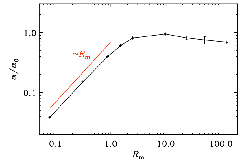
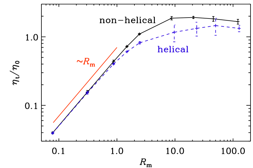
As theoretically expected (Moffatt 1978, Krause & Rädler 1980), and previously demonstrated using the test-field method (Sur et al. 2008), $\alpha$ and $\eta$ increase linearly with $R_{\rm m}$ for $R_{\rm m}<1$; see Figs. 1 and 2 for nonhelical and helical cases. Here, error bars have been evaluated as the maximum departure from the averages for any one third of the full time series. In the helical case, both $\alpha$ and $\eta$ saturate around unity, but in the non-helical case, $\eta$ overshoots the helical value by almost a factor of two; see Fig. 2.

3.2 Ratio of $\alpha$ to $\eta_{\rm t}$

In Fig. 3, we plot the ratio $\eta_{\rm t}/\alpha$, normalized by $\eta_{\rm t0}/\alpha_{0}$, where $\alpha_{0}=-u_{\rm rms}/3$ and $\eta_{\rm t0}=u_{\rm rms}/3k_{\rm f}$. The minus sign in our expression for $\alpha_{0}$ takes into account that we are forcing with positive helicity, which then leads to a negative $\alpha$ effect (Moffatt 1978, Krause & Rädler 1980). For small values of $R_{\rm m}$, this ratio is unity, but it reaches a value of about two when $R_{\rm m}\approx 50$.

Figure 1: Dependence of $\alpha$ on $R_{\rm m}$ for the models with maximum helicity.

Figure 2: Dependence of $\eta_{\rm t}$ on $R_{\rm m}$ for models with maximum helicity (dashed blue) and with zero helicity (solid black).

Figure 3: Ratio of $\eta_{\rm t}/\alpha$.

Figure 4: $R_{\rm m}$ dependence of the difference between $\eta_{\rm t}$ for models with zero helicity an maximum helicity.

3.3 Difference between nonhelical and helical cases

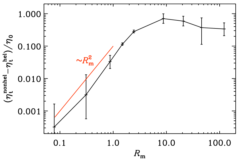
It turns out that the difference between $\eta_{\rm t}$ in the nonhelical and helical cases increases quadratically in $R_{\rm m}$; see Fig. 4. This shows first of all that the difference vanishes for small $R_{\rm m}$, but it also suggests that there is a correction to $\eta_{\rm t}$ due to the presence of helicity that is not captured by the second order correlation approximation, which is exact for $R_{\rm m}\ll 1$. It should be possible, however, to capture this effect of helicity on $\eta_{\rm t}$ using a higher order approximation, which has not yet been attempted, however.

3.4 Relation to earlier results

A similar situation has been encountered previously in the case of the Galloway–Proctor flow (Galloway & Proctor 1992), where, in addition to an $\alpha$ effect and turbulent diffusion, also a turbulent pumping effect was found (Courvoisier et al. 2006). This result was not obtained under the second order correlation approximation (Rädler & Brandenburg 2009). Using the test-field method, they showed, however, that the value of $\gamma$, which quantifies the turbulent pumping velocity, does indeed vanish for $R_{\rm m}\ll 1$, but it was found to increase with $R_{\rm m}$ as $R_{\rm m}^{5}$; see Rädler & Brandenburg (2009), who interpreted this as a higher order effect that should be possible to capture with a six order approximation. Our present result therefore suggests that the difference between nonhelical and helical cases can also be described as a result of a higher order approximation, which, in this case, would be a fourth order approximation.

4 Conclusions

Our present results have demonstrated that, at least for intermediate values of $R_{\rm m}$ in the range between 1 and 120, there is a contribution to the usual expression for the turbulent magnetic diffusivity $\eta_{\rm t}=\tau\overline{\bm{u}^{2}}/3$ that depends on $(\overline{\bm{\omega}\cdot\bm{u}})^{2}$. This is somewhat surprising in the sense that such a result has not previously been reported, but it is fully compatible with all known constraints: no correction for $R_{\rm m}\ll 1$ and no dependence on the sign of $\overline{\bm{\omega}\cdot\bm{u}}$. On the other hand, our results may still be compatible with the $\tau$ approximation in the high conductivity limit, if the difference between the turbulent diffusivity in the nonhelical and helical cases vanishes for $R_{\rm m}\to\infty$. However, our numerical results do not clearly confirm this, because our largest value of $R_{\rm m}$ was only about 120.

There is a practically relevant application to this phenomenon, at least in the case of forced turbulence, where its effect on the large-scale magnetic field evolution can now be quantified to high accuracy. A factor of nearly two in the value of $\eta_{\rm t}$ is clearly beyond the acceptable accuracy for this case. This was noticed in recent studies of $\alpha$ effect and turbulent diffusion in the presence of the chiral magnetic effect (Schober et al. 2017). Our present result therefore removes an otherwise noticeable discrepancy relative to the theoretical predictions. Future applications hinge obviously on the overall accuracy of analytic approximations to particular circumstances. In most cases, naturally driven flow turbulence will be anisotropic, so we expect more complicated tensorial results for turbulent diffusion.