Asymptotic approximation
of the Wigner function
in two-phase geometric optics

ASYMPTOTIC APPROXIMATION
OF THE WIGNER FUNCTION
IN TWO-PHASE GEOMETRIC OPTICS

A MASTER THESIS
SUBMITTED TO THE PROGRAM IN
“MATHEMATICS AND ITS APPLICATIONS”
OF UNIVERSITY OF CRETE

I certify that I have read this thesis and that, in my opinion, it is fully adequate in scope and quality as a thesis for the degree of Master of Science.

  (George N. Makrakis) Principal Adviser

I certify that I have read this thesis and that, in my opinion, it is fully adequate in scope and quality as a thesis for the degree of Master of Science.

  (Stathis Filippas)

I certify that I have read this thesis and that, in my opinion, it is fully adequate in scope and quality as a thesis for the degree of Master of Science.

  (George Kossioris)

Approved for the Program Committee.

Abstract

We propose a renormalization process of a two phase WKB solution, which is based on an appropriate surgery of local uniform asymptotic approximations of the Wigner transform of the WKB solution. We explain in details how this process provides the correct spatial variation and frequency scales of the wave field on the caustics where WKB method fails. The analysis has been thoroughly presented in the case of a fundamental problem, that is the semiclassical Airy equation, which arises from the model problem of acoustic propagation in a layer with linear variation of the sound speed.

Chapter 1 Introduction

High-frequency wave propagation in inhomogeneous media, has been traditionally investigated employing the method of geometrical optics. Not only it is used to draw a qualitative picture of how the energy propagates, but also to evaluate the wave fields quantitatively. However, geometrical optics fails either on caustics and focal points where it predicts infinite wave amplitudes, or in shadow regions (i.e. regions devoid of rays) where it yields zero fields. On the other hand, formation of caustics is a typical situation in optics, underwater acoustics and seismology, as a result of multipath propagation from localized sources. Indeed, even in the simplest oceanic models and geophysical structures (see, e.g. Tolstoy and Clay [TC], Chapt. 5, and Cĕrvenỳ, et.al. [CMP], Chapt. 3, respectively) a number of caustics occur, depending upon the position of the source and the stratification of the wave velocities.

1.1 Caustics and phase-space methods

Mathematically, caustic surfaces are envelopes of rays. Physically, these surfaces are distinctive in that the field intensity increases on them sharply as compared with the adjacent regions. The rise of field is best of all seen at the focal points where all the rays corresponding to the converging wave front intersect.

In his classical book Stavroudis [Sta] has remarked that in contrast to rays and wave fronts, the caustic is one of the few objects in optics that can be observed in reality. This remark emphasizing the role of caustics, of course, has its own range of validity, and it is true only to the point that in the close vicinity of caustics, one can observe or measure a concentration of the field. Is the caustic real in the above sense in all situations, i.e., is the effect of field buildup on a caustic appreciable enough for instruments to reveal, separate and identify the caustics? This question may be answered with heuristic criteria. A caustic may be deemed real, i.e., observed or recorded, if the amplitude on the caustic is at least a few times the mean field value elsewhere and the near-caustic zones of adjacent caustics do not completely overlap. Some other conditions of practical character like, noise should not be high, resolution and sensitivity of the instruments should be sufficient, should be satisfied.

Moving across a caustic gives birth or annihilation of a pair of rays at a time, and this discontinuous variation of the number of rays across a caustic is qualified as a catastrophe. This new and fruitful approach to caustics, developed only in the recent years, allows a universal classification of the typical caustics (see, e.g., [KO1]).

From specific examples allowing exact solutions, it has been known that the phase of the wave fields change by $-\pi/2$ upon touching a smooth (nonsingular) caustic, and by $-\pi$ after passing a three-dimensional focus. However, a universal rule on the additional phase shift at a caustic has been formulated only in the comparative recent works of Maslov ([Ma1], [Ma2]) and Lewis [Le], although the germ of the idea goes back to Keller [Kel]. The formulation is based on the stationary-phase approximation of certain diffraction integrals, and it finally leads to the notion of the so-called Maslov trajectory index, in the general case of multiple caustic reflections.

Because the wave amplitude predicted by geometrical optics is infinite on the caustics, as a result of ray convergence, geometrical optics is inapplicable within a close neighborhood of the caustic, as actual wave fields are always finite. However, available exact and approximate solutions for certain canonical wave problems involving caustics in the high-frequency limit, indicate a substantial concentration of energy near a caustic. This phenomenon is more profound within a finite region which is usually referred as caustic zone or caustic volume. The rigorous estimation of the size of this zone should rely upon delicate uniform asymptotic expansions of certain canonical diffraction integrals associated with the particular caustic, but for the moment only heuristic estimations leading rather to qualitative than to fully quantitative results exist. A very important feature is that the rays cannot be adequately resolved in the caustic zone, and therefore we can draw the general conclusion that within any caustic zone, no physical device is capable of separate determination of ray parameters. In this sense, in that caustic zone, rays loose their physical individual properties, though they continue to play the role of the geometric framework for the wave field.

From the mathematical point of view, formation of caustics and the related multivaluedness of the phase function, is the main obstacle in constructing global high-frequency solutions of the wave equation. The problem of obtaining the multivalued phase function is traditionally handled by resolving numerically the characteristic field related to the eikonal equation (ray tracing methods), see, e.g. [CMP]. A considerable amount of work has been done recently on constructing the multivalued phase function by properly partitioning the propagation domain and using eikonal solvers (see, e.g., [Ben], [FEO]).

Given the geometry of the multivalued phase function, a number of local and uniform methods to describe wave fields near caustics have been proposed. The local methods are essentially based on boundary layer techniques as they were developed by Babich, Keller, et.al. (see, e.g., [BaKi], [BB]). The uniform are those which exploit the fact that even if the family of rays has caustics, there are no such singularities for the family of the bicharacteristics in the phase space. This basic fact allows the construction of formal asymptotic solutions (FAS) which are valid also near and on the caustics. For this purpose two main asymptotic techniques have been developed. The first one is the Kravtsov-Ludwig method (sometimes called the method of relevant functions). This method starts with a modified FAS involving Airy-type integrals, the phase functions of which take account of the particular type of caustics. The second one is the method of the canonical operator developed by Maslov. The construction of the canonical operator exploits the fact that the Hamiltonian flow associated with the bichararcteristics generates a Lagrangian submanifold in the phase space, on which we can “lift” the phase function in a unique way (see, e.g., [MF],[MSS],[Va1]).

Although uniform caustic asymptotics have been widely used by the acoustical and seismological community (see, e.g., [CH1], [CH2] and the references cited there), the problem of the limits of applicability of uniform asymptotic expressions has not been completely resolved yet, as it has been observed by Asatryan and Kravtsov [AsK] who attempted to give a qualitative answer. Note also that apart from their importance in the qualitative description of wavefields near caustics, the Kravtsov-Ludwig solutions have been also proved useful for numerical computations through appropriate matching with geometric optics far away from the caustics [KKM].

1.2 The Wigner-function approach

A relatively new technique to treat high frequency dispersive problems is based on the Wigner transform of the wavefunction, whose basic properties (i.e. the relation of its moments with important physical quantities, as energy density, current density, et.al.), make it a proper and extremely useful tool for the study of the wavefield. Wigner function is a phase space object satisfying an integro-differential equation (Wigner equation), which for smooth medium properties can be expressed as an infinite order singular perturbation (with dispersion terms with respect to the momentum of the phase space)of the classical Liouville equation. At the high frequency limit the solution of the Wigner equation equation converges weakly to the so called Wigner measure [LP] governed by the classical Liouville equation, and this measure, in general, reproduces the solution of single phase geometrical optics.

We should note at this point that there does not exist, up to now, either some systematic theoretical study of the Wigner integro-differential equation (except the results of Markowich [SMM] for the equivalence of Wigner and Schrödinger equations). This is due to fundamental difficulties of this equation, which is an equation with non-constant coefficients, that combines at least two different characters, that of transport and that of dispersive equations. The first character is correlated with the Hamiltonian system of the Liouville equation (and the classical mechanics of the problem), and the second with the quantum energy transfer away from the Lagrangian manifold of the Hamiltonian system, but mainly inside a boundary layer around it, the width of which depends on the smoothness of the manifold and the presence or not of caustics.

Moreover, in the case of multi-phase optics and caustic formation, Wigner measure is not the appropriate tool for the study of the semi-classical limit. In fact ut has been shown by Filippas & Makrakis [FM1], [FM2] through examples in the case of time-dependent Schrodinger equation that the Wigner measure (a) it cannot be expressed as a distribution with respect to the momentum for a fixed space-time point, and thus cannot produce the amplitude of the wavefunction, and (b) it is unable to “recognize” the correct frequency dependencies of the wavefield near caustics. It was however explained that the solutions of the integro-differential Wigner equation do have the capability to capture the correct frequency scales. It must be said here that a numerical approach based on classical Liouville equation has been developed, as an alternative to WKB method, in order to capture the multivalued solutions far from the caustic. This technique is based on a closure assumption for a system of equations for the moments of the Wigner measure (essentially by assuming a fixed number of rays passing through a particular point) (see, e.g., ([JL], [Ru1], [Ru2]).

1.3 The present work: Renormalization of WKB solutions

In the present work we employ Wigner transform as a tool for the renormalization of WKB solutions near caustics (wignerization). More precisely, we consider the fundamental example of the semiclassical Airy equation, whose two-phase WKB solution fails at the caustic (namely the turning point of the Airy equation) due to the divergence of the geometric amplitudes. We show that the combination (“surgery”) of appropriate asymptotic approximations of the Wigner function in various areas of the phase space leads to an approximate Wigner function which recovers the correct semiclassical (Airy) amplitude in a spatially uniform way. Moreover, the interaction mechanism between the two geometric phases (realized as the two branches of the folded Lagrangian manifold) is investigated by thoroughly analyzing the structure of the stationary points of the corresponding cross Wigner integrals and their asymptotic contribution in the Airy structure. Note that for our particular examples, it happens that the asymptotics of the Wigner function leads to the exact Wigner transform of the semiclassical Airy function, which confirms the validity of the proposed wignerization. It should be emphasized that the proposed renormalization process has many similarities and it has been inspired by the so-called quantization processes (see, e.g., Nazaikinskii et al [NSS]), since we can consider the WKB solution as the “classical object” and the constructed approximation of the Wigner function as the “quantum object”. It is then interesting to observe that in the full high-frequency limit the approximation of the Wigner function, the quantum object, gives us back the WKB solution, that is the classical object.

The structure of the work is the following. In Chapter 2 we present the technique of geometric optics(WKB solutions) and the method developed by Kravtsov & Ludwig. We also analyze the propagation of plane acoustic waves in a layer with linear variation of the reafraction index, we construct the WKB and Kravtsov-Ludwig solutions and we explain how the semiclassical Airy eqaution bounces out of this model. In Chapter 3 we introduce the Wigner transform, we review its basic properties and we also present in details Berry’s construction of the semiclassical Wigner function. In Chapter 4, which is our main contribution, we construct the asymptotics of the Wigner transform of the WKB solution of the semiclassical Airy equation and we make some remarks on the stationary Wigner function and the possibility of generalizing our process in problems with more complicated refraction indices as well in two-dimensional propagation problems where folds can also appear. Finally, in a series of four appendices we briefly append basic results for the uniform stationary phase method and the idea of the parametrization of the Lagrangian manifold used by Kravtsov and Ludwing in the derivation of their asymptotic formula.

Chapter 2 Geometrical optics

2.1 The WKB method

We consider the propagation of $n$-dimensional time-harmonic acoustic waves in a medium with variable refraction index $\eta(\textbf{x})=c_{0}/c(\textbf{x})$, $c_{0}$ being the reference sound velocity and $c(\textbf{x})$ the wave velocity at the point ${\bf{x}}=(x_{1},...,x_{n})\in M$, where $M$ is some unbounded domain in $R^{n}_{\bf{x}}$. We assume that $\eta\in C^{\infty}({R^{n}_{\bf{x}}})$ and $\eta>0$. The wave field $u(\bf{x},\kappa)$ is governed by the Helmholtz equation

$$\Delta u(\textbf{x},\kappa)+\kappa^{2}{\eta}^{2}({\textbf{x}})u({\bf{x}},\kappa)=f(\textbf{x})\ ,\quad{\bf{x}}\in M\ ,$$ (2.1)

where $\kappa=\omega/c_{0}$ is the wavenumber ($\omega$ being the frequency of the waves) and $f$ is a compactly supported source generating the waves. We are interested in the asymptotic behavior of $u(\bf{x},\kappa)$ as $\kappa\to\infty$ (i.e. for very large frequencies $\omega$) , assuming that $\bf{x}$ remains in a compact subset of $M$. Note that the asymptotic decomposition of scattering solutions when simultaneously $|\textbf{x}|$ and $\kappa$ go to infinity is a rather complicated problem, as, in general, the caustics go off to infinity. This problem has been rigorously studied in Vainberg [Va], when $M$ is a full neighborhood of infinity and $\eta=1$ for $|\textbf{x}|>r_{0}$ , $r_{0}$ being a fixed positive constant, and by Kucherenko [Ku] for the case of a point source (i.e., $f(\bf{x})=\delta(\bf{x})$) , under certain conditions of decay for $\eta(\bf{x})$ as $|\bf{x}|\to\infty$ .

For fixed $\kappa>0$ there is, in general, an infinite set of solutions of (2.1), and we thus need a radiation condition to guarantee uniqueness (cf. [CK] for scattering by compact inhomogeneities, and [Wed] for scattering by stratified media). This condition is essentially equivalent to the assumption that there is no energy flow from infinity, which in geometrical optics is translated to the requirement that the rays must go off to infinity (cf. [PV], [Ca]).

• We say that

  $$u_{N}({\bf{x}},\kappa)=e^{i\kappa S(\bf{x})}\sum_{\ell=0}^{N}(i\kappa)^{-\ell}A_{\ell}(\bf{x})\ ,$$ (2.2)

  where the phase $S$ and the amplitudes $A_{\ell}$ are real-valued functions in $C^{\infty}(R^{n}_{\bf{x}})$ , is a formal asymptoptic solution (FAS) of $(\ref{helm})$, if it satisfies the asymptotic equation

  $$(\Delta+\kappa^{2}\eta^{2}({\bf{x}}))u_{N}({\bf{x}},\kappa)=O(\kappa^{-N_{1}})\ ,\quad\kappa\to\infty\ ,$$ (2.3)

  with $N_{1}\rightarrow\infty$ as $N\rightarrow\infty$ , in a bounded domain $|\textbf{x}|\leq a$ , $a$ being a positive constant.

According to the WKB procedure, we seek a FAS of $(\ref{helm})$ in the form $(\ref{asexp})$. Substituting $(\ref{asexp})$ into $(\ref{approxhelm})$, and separating the powers $(i\kappa)^{-\ell},\thinspace\ell=0,1,\dots$ , we obtain the eikonal equation

$$\left(\nabla S(\bf{x})\right)^{2}=\eta^{2}(\bf{x})\ ,$$ (2.4)

for the phase function, and the following hierarchy of transport equations

$$2\nabla S({\bf{x}})\cdot\nabla A_{0}({\bf{x}})+\Delta S({\bf{x}})A_{0}({\bf{x}})=0\ ,$$ (2.5)

$$2\nabla S({\bf{x}})\cdot\nabla A_{\ell}({\bf{x}})+\Delta S({\bf{x}})A_{\ell}({\bf{x}})=-\Delta A_{\ell-1}({\bf{x}}),\ \ell=1,2,\dots\ ,$$ (2.6)

for the principal and higher-order amplitudes, $A_{0}$ and $A_{\ell}$ , respectively.

2.2 Rays and Caustics

A standard way for solving the eikonal equation $(\ref{eikonal})$ is based on the use of bicharacteristics (see, e.g., [Ho], Vol. I, Chap. VIII, and [Jo], Chap. 2). Let $H(\bf{x},\bf{k})$ be the Hamiltonian function

$$H(\textbf{x},\textbf{k})=\frac{1}{2}\left(\textbf{k}^{2}-\eta^{2}(\textbf{x})\right),\quad\textbf{x}\in M,\quad\textbf{k}\in R^{n}\ ,$$ (2.7)

corresponding to the Helmholtz equation $(\ref{helm})$, where $\textbf{k}=(k_{1},...,k_{n})$ is the momentum, conjugate to the position $\textbf{x}=(x_{1},...,x_{n})$ .

The associated Hamiltonian system reads as follows

$$\frac{d\bf{x}}{dt} = \nabla_{\bf{k}}H(\bf{x},\textbf{k})=\textbf{k}\ ,$$

$$\frac{d\textbf{k}}{dt} = -\nabla_{\bf{x}}H(\bf{x},\textbf{k})=\eta(\bf{x})\cdot\nabla_{\bf{x}}\eta(\bf{x})\ .$$ (2.8)

Here, since we deal with a time-independent problem, $t$ is simply a time-like parameter which parametrizes the trajectories. For $\textbf{k}=\nabla_{\bf{x}}S(\bf{x})$ , we see that $H(\textbf{x},\textbf{k})=0$ gives just the eikonal equation $(\ref{eikonal})$.

Let now $\Lambda_{0}$ be a manifold of dimension $n-1$ in $R^{n}$ ,

$$\Lambda_{0}=\{\textbf{x}=\textbf{x}_{0}(\theta)\ ,\ \theta=(\theta_{1},...,\theta_{n-1})\in U_{0}\subseteq{R}^{n-1}\}\ .$$

For $t=0$ we specify on $\Lambda_{0}$ the following initial conditions

$$\textbf{x}(0)=\textbf{x}_{0}(\theta)\ ,\quad\textbf{k}(0)=\textbf{k}_{0}(\theta)\ ,\quad\theta\in U_{0}\ ,$$ (2.9)

for the Hamiltonian system $(\ref{hamsys})$, and for this reason, in the sequel, we refer to $\Lambda_{0}$ as the initial manifold (from which the bicharacteristics depart).

Also, we assume the initial conditions

$$S(\textbf{x})=S_{0}(\theta)\ ,\quad A_{l}(\textbf{x})=\alpha_{l}(\theta)\quad\mathrm{for}\quad\textbf{x}=\textbf{x}_{0}(\theta)\in\Lambda_{0}\ ,$$ (2.10)

for the phase and the amplitudes, $S_{0}(\theta)$ , $\alpha_{l}(\theta)$ being given smooth functions on the initial manifold $\Lambda_{0}$ . Note that $\textbf{k}_{0}(\theta)$ must satisfy the condition

$${\mid\textbf{k}_{0}(\theta)\mid}^{2}=\Bigl{(}\eta(\textbf{x}_{0}(\theta))\Bigr{)}^{2},\quad\textbf{x}_{0}\in\Lambda_{0}\ ,$$ (2.11)

for the eikonal to be satisfied also at $t=0$ .

• The trajectories $\left\{\textbf{x}=\textbf{x}(t,\theta)\ ,\ \textbf{k}=\textbf{k}(t,\theta)\ ,\ t\in R\ ,\ \theta\in U_{0}\right\}$ which solve the initial value problem $(\ref{hamsys})$, $(\ref{initbich})$, in the phase space $R_{\bf{x}\bf{k}}^{2n}$ are called bicharacteristics, and their projection $\{\textbf{x}=\textbf{x}(t,\theta)\ ,\ t\in R\ ,\ \theta\in U_{0}\}$ onto $R_{\bf{x}}^{n}$ are called rays.

The initial manifold $\Lambda_{0}$ evolves under the Hamiltonian flow defined by the bicharecteristics to the manifold

$$\Lambda_{t}=\Bigl{\{}\bigl{(}\textbf{x}(t,\theta),\textbf{k}(t,\theta)\bigr{)}\ ,\ \theta\in U_{0}\ ,\ t\geq 0\Bigr{\}}\ .$$

Obviously, since $\textbf{k}=\nabla_{\textbf{x}}S$ , the bicharacteristics lie on the manifold $H({\textbf{x}},{\textbf{k}})=0$ , thanks to the eikonal equation, and therefore $\Lambda_{t}$ is a subset of the constant-energy manifold $H({\bf{x}},{\textbf{k}})=0$ for any $t\geq 0$ . Moreover, in order to the eikonal to be satisfied for $t=0$ , it must be $\textbf{k}_{0}=\nabla_{{\bf{x}}}S_{0}(\textbf{x})$ and therefore $\Lambda_{0}$ has the important property that it is a Lagrangian manifold in the phase space $R_{\bf{x}\bf{k}}^{2n}$ (see, the book by Maslov & Fedoryuk [MF] for a detailed introduction to the theory of Lagrangian manifolds and its relation to the construction of asymptotics, and also the expository paper by Littlejohn [Lit]). This property remains invariant under the Hamiltonian flow, and therefore $\Lambda_{t}$ remains Lagrangian for all $t\geq 0$ .

Also, in the sequel, we will assume that that $\textbf{k}_{0}(\theta)$ is nowhere tangent to $\Lambda_{0}$ in order to the (non-characteristic) Cauchy problem for the eikonal equation have a smooth unique solution for small $t$ (see, e.g. Courant & Hilbert [CH], Vol. II, Chap. II ).

Now, using the first equation of the Hamiltonian system $(\ref{hamsys})$

$$\frac{d\textbf{x}}{dt}=\textbf{k}=\nabla S_{{\bf{x}}}\\$$ (2.12)

we see that $S$ satisfies the following ordinary differential equation

$$\frac{dS(\textbf{x})}{dt}=\nabla_{{\bf{x}}}S\cdot\frac{d\textbf{x}}{dt}=\textbf{k}\frac{d\textbf{x}}{dt}=|\textbf{k}|^{2}=\eta^{2}(\textbf{x})\ .$$ (2.13)

Integrating the last equation along the rays, we obtain the phase

$$S(\textbf{x}(t,\theta))=S_{0}(\theta)+\int_{0}^{t}\eta^{2}(\textbf{x}(\tau,\theta))d\tau\ .$$ (2.14)

The solution of the transport equation $(\ref{transport})$ for the principal amplitude $A_{0}$ along the rays, is obtained by applying divergence theorem in a ray tube $T_{t}$ . Assuming that $A_{0}$ is finite and non-zero, the transport equation $(\ref{transport})$ is rewritten in the divergence form

$$\nabla\cdot({A_{0}}^{2}\nabla S)=0\ ,$$ (2.15)

and integrating on the ray tube $T_{t}$ with boundary $\partial T_{t}=\Sigma_{0}\cup\Sigma_{0t}\cup\Sigma_{t}$ , we have

$$0=\int_{T_{t}}\nabla\cdot({A_{0}}^{2}\nabla S)\,dT=\int_{\partial T_{t}}{A_{0}}^{2}(\nabla S\cdot\vec{\nu})\,d\Sigma$$

where $\vec{\nu}$ the unit outer normal vector on the boundary $\partial{T_{t}}$ of $T_{t}$ , and $d\Sigma$ is surface element.

Now, since the rays have the direction of $\nabla S$ , that is, the rays are perpendicular to the wave fronts $S=$ const. , the vectors $\vec{\nu}$ and $\nabla S$ are orthogonal on the lateral boundary $\Sigma_{0t}$ of the ray tube, and we therefore obtain

$$0=\int_{\partial T_{t}}{A_{0}}^{2}(\nabla S\cdot\vec{\nu})\,d\Sigma = \int_{\Sigma_{0}}\alpha_{0}^{2}(\nabla S\cdot\vec{\nu})\,d\Sigma_{0}+\int_{\Sigma_{t}}{A_{0}}^{2}(\nabla S\cdot\vec{\nu})\,d\Sigma_{t}$$ (2.16)

$$= -\int_{\Sigma_{0}}\alpha_{0}^{2}|\textbf{k}_{0}|\,d\Sigma_{0}+\int_{\Sigma_{t}}{A_{0}}^{2}|\textbf{k}|\,d\Sigma_{t}\ .$$

Then, we have

$$-\alpha_{0}^{2}|\textbf{k}_{0}|\,d\Sigma_{0}+{A_{0}}^{2}|\textbf{k}|\,d\Sigma_{t}=0$$

that gives

$${A_{0}}^{2}=\alpha_{0}^{2}\frac{|\textbf{k}_{0}|}{|\textbf{k}|}\frac{d\Sigma_{0}}{d\Sigma_{t}}=\frac{\alpha_{0}^{2}}{J}$$ (2.17)

where

$$J=J(t,\theta)=\frac{D(t,\theta)}{D(0,\theta)}\ ,\qquad D(t,\theta)=\det\frac{\partial\textbf{x}(t,\theta)}{\partial(t,\theta)}\ ,$$ (2.18)

is the Jacobian of the ray transformation $(t,\theta)\mapsto\textbf{x}(t,\theta)$ (see, e.g., [BB], [Zau]).

Therefore we derive the principal amplitude

$$A_{0}(\textbf{x}(t,\theta))=\frac{\alpha_{0}(\theta)}{\sqrt{J(t,\theta)}}$$ (2.19)

where $A_{0}(\textbf{x}(t=0,\theta))=\alpha_{0}(\theta)$ is the amplitude at the point $\textbf{x}=\textbf{x}_{0}(\theta)$ on the initial manifold $\Lambda_{0}$ .

• An alternative way to derive the formula $(\ref{amplitude})$ starts form the Liouville formula [Ha]

$$\frac{d}{dt}\ln\frac{D(t,\theta)}{D(0,\theta)}=\sum_{i=1}^{n}{\frac{\partial k_{i}}{\partial x_{i}}}=\sum_{i=1}^{n}{\frac{\partial^{2}S}{\partial x_{i}^{2}}}=\Delta S$$ (2.20)

which, since $D(0,\theta)=1$ , implies

$$\frac{d}{dt}\ln{D(t,\theta)}=\Delta S\ .$$ (2.21)

From the transport equation $(\ref{transport})$ we have

$$-\Delta S=\frac{2}{A_{0}}\nabla S\cdot\nabla A_{0}$$

and since

$$\frac{d}{dt}\ln{A_{0}}^{2}=\frac{2}{A_{0}}\frac{dA_{0}}{dt}=\frac{2}{A_{0}}\nabla A_{0}\frac{d\textbf{x}}{dt}=\frac{2}{A_{0}}\nabla A_{0}\cdot\nabla S$$

it follows

$$\frac{d}{dt}\ln{A_{0}}^{2}=-\Delta S\ .$$

Then using $(\ref{smirn})$ we get

$$\frac{d}{dt}\ln{A_{0}}^{2}=-\frac{d}{dt}\ln D(t)\ ,$$

which after integration on the interval $(0,t)$ leads to the formula $(\ref{amplitude})$ for the principal amplitude.

The higher-order amplitudes can be also derived by integrating the hierarchy of transport equations $(\ref{htransport})$ in a similar way.

The transformation

$$(t,\theta)\mapsto\textbf{x}(t,\theta)\ ,$$

is one-to-one, provided that the determinant of the Jacobian

$$D(t,\theta)=\det\frac{\partial(x_{1},...,x_{n})}{\partial(t,\theta_{1},...,\theta_{n-1})}\ ,$$

is non-zero. Note that $D(t,\theta)$ is non-zero since we have excluded the possibility of the characteristics to be tangent to $\Lambda_{0}$ at $t=0$ . But even if $D(t=0,\theta)\neq 0$ , $D(t,\theta)$ and therefore $J(t,\theta)$ , it does not necessarily remain non-zero for all $t$ . Whenever $J=0$ , it can happen that $(t,\theta)$ may be non-smooth or multi-valued functions of x, and the rays may intersect, touch, and in general have singularities, although the bicharacteristics never develop such singularities in the phase space. Then, the phase function $S=S(\textbf{x}(t,\theta))$ may be a multi-valued or even a non-smooth function. It must be emphasized that in the neighborhoods of the singular points we cannot choose the coordinates $x_{1},\ldots,x_{n}$ as local coordinates.

• The points $\textbf{x}=\textbf{x}(t,\theta)$ at which $J(t,\theta)=0$ , are called focal points, and the manifold generated from these points, that is, the envelope of the family of the rays, is called caustic.

It follows from (2.19), that the principal amplitude $A_{0}$ blows up on the caustics. However, it is known that solutions of the Helmholtz equation are analytic away form source points and it is therefore the WKB procedure for constructing the (FAS) which fails to predict the correct amplitudes on the caustics. From the geometrical point of view, this non-physical blow up of the amplitude at the caustic is associated with the diminishing of the ray tubes there (the ray tube cross section $\Sigma_{t}$ vanishes whenever the ray touches the caustic), and it is clearly a consequence of the way of solving the transport equation by integrating along the rays. In fact, a boundary layer analysis [BaKi], [BuKe] shows that the ray structure breaks down near the caustic, and within a boundary layer the modal structure of the wave field is dominant, which makes therefore impossible to separate the waves approaching the caustic from those leaving from it. However, uniform asymptotic solutions which will be considered in the sequel, show that it exists considerable energy concentration near the caustic, which makes it detectable, but the field is spatially finite but strongly increasing with increasing frequency.

Asymptotic methods for calculating finite fields on the caustics have been developed by Kravtsov [Kra], [KO] and Ludwig [Lu] (the method of relevant functions) and by Maslov [MF](the method of the canonical operator). Although the two methods have been developed along different lines, they are both essentially based on the symplectic properties of the Lagrangian manifold $\Lambda_{t}$ . We will briefly present the Kravtsov-Ludwig technique. A relatively recent way to treat high frequency problems is based on the Wigner transform of the wavefunction, whose basic properties (i.e. the relation of its moments with important physical quantities, as energy density, current density, et.al.), make it a proper and extremely useful tool for the study of the wavefield. Wigner function is satisfying an integro-differential equation in phase space, which for smooth potential functions can be expressed as an infinite order singular perturbation (with dispersion terms with respect to the momentum of the phase space), of the classical Liouville equation.

At the high frequency limit, the solution of Liouville equation converges weakly to the so called Wigner measure [LP], which for relatively smooth initial phase functions $S_{0}$ produces the solution of single phase geometrical optics. But in the case of multi-phase optics and caustic formation, Wigner measure is not the appropriate tool for the study of the semi-classical limit, because as is shown through examples for the time-dependent Schrodinger equation by Filippas & Makrakis [FM1], [FM2] (a) it cannot be expressed as a distribution with respect to the momentum for a fixed space-time point, and thus cannot produce the amplitude of the wavefunction, and (b) it is unable to “recognize” the correct dependencies of the wavefield from the semiclassical parameter $\epsilon$ near caustics. This is a property that the solutions of the integro-differential Wigner equation do have.

We should note that up to now, there does not exist either some systematic theoretical study of the Wigner integro-differential equation (except the results of Markowich [SMM] for the equivalence of Wigner and Schrödinger equations), neither some method for constructing solutions or their representations. This is due to fundamental difficulties of this equation, which is an equation with non-constant coefficients, that combines at least two different characters, that of transport and that of dispersive equations. The first character is correlated with the Hamiltonian system of the Liouville equation (and the classical mechanics of the problem), and the second with the wave energy transfer away from the Lagrangian manifold of the Hamiltonian system- mainly inside a boundary layer around the manifold- the width of which depends on the smoothness of the manifold and the presence or not of caustics.

2.3 The Kravtsov-Ludwig technique

2.3.1 Motivation and heuristic foundation

The idea of obtaining global high-frequency solutions of the Helmholtz equation $(\ref{helm})$ by the method of relevant functions, is to replace $(\ref{asexp})$ by integrals of the form (see, e.g., the classical paper by Ludwig [Lu], the modern approach by Duistermaat [Dui1], [Dui2], also the book by Guillemin & Sternberg [GS])

$$u(\textbf{x},\kappa)=\left(\frac{i\kappa}{2\pi}\right)^{\frac{1}{2}}\int_{\Xi}e^{i\kappa S\left(\bf{x},\xi\right)}\,A(\textbf{x},\xi)\,d\xi\ ,\quad\textbf{x}\in M\subseteq R_{\bf{x}}^{n}\ ,\quad\xi\in\Xi\subseteq R_{\xi}\ .$$ (2.22)

where the phase $S(\textbf{x},\xi)$ and the amplitude $A(\textbf{x},\xi)$ must satisfy the eikonal equation $(\ref{eikonal})$ and the transport equation $(\ref{transport})$, respectively, identically with respect to $\xi$. Here, the term global solution means that the integral representation holds uniformly away and on the caustics.

The integral $(\ref{intexp})$ can be regarded as a continuous superposition of oscillatory functions of the form $(\ref{asexp})$. The underlying physical motivation is the fact that in every small region in which the refraction index of the medium can be approximately considered as constant, and the wave front as plane, the field can be represented as a superposition of plane waves $Ae^{i\kappa S}$ , where the local amplitude $A$ and the local wavenumber $\nabla_{\bf{x}}S$ vary slowly in transition from one region to the next.

The phase $S(\textbf{x},\xi)$ parametrizes the Lagrangian submanifold $\Lambda_{t}$ generated by the corresponding Hamiltonian flow, in the sense that $\Lambda_{t}$ is locally represented by $(\textbf{x},\textbf{k})=(\textbf{x},\nabla_{\bf{x}}S(\textbf{x},\xi))$ . In the language of microlocal analysis, the representation $(\ref{intexp})$ defines a Lagrangian distribution on $\Lambda$, which for large $\kappa$ is an asymptotic solution (compound asymptotics) of the Helmholtz equation (see the book by Guilllemin and Sternberg [GS] for a detailed but rather technical exposition of this technique). In this sense, the construction of an asymptotic expansion in the form $(\ref{intexp})$ is “equivalent” with the construction of the Lagrangian submanifold $\Lambda$. Near caustics $S(\textbf{x},\xi)$ is a multivalued function and, in general, it cannot be derived by integration along the bicharacteristics by simply applying $(\ref{gphase})$. Representation formulae for the phase function $S(\textbf{x},\xi)$ are constructed, for each caustic which is generated from the particular ray system (different caustics may appear for the same Hamiltonian with different initial data), by appealing, in general, to the methods of singularity theory (see, e.g., [AVH]). For a simple fold caustic this construction is relatively simple, and we briefly present it in the next section.

First of all, in the case of single-phase geometrical optics, we can take $S(\textbf{x},\xi)=\phi(\textbf{x})-\xi^{2}$ . Then, $\partial_{\xi}S(\textbf{x},\xi)=-2\xi$ , and there is only a simple stationary point $\xi=0$. By the standard stationary phase lemma (see, e.g., [BH], p. 219), the oscillatory integral $(\ref{intexp})$ reduces asymptotically to $(\ref{asexp})$. If there are more than one simple stationary points $\xi_{j}(\textbf{x})$ , that is, $\partial_{\xi}S(\textbf{x},\xi_{j}(\textbf{x}))=0$ and $\partial_{\xi}^{2}S(\textbf{x},\xi_{j}(\textbf{x}))\neq 0$ , we obtain the asymptotic expansion

$$u({\bf{x}},\kappa)\sim\sum_{j=1}^{j=J}A_{0}^{j}({\bf{x}})e^{i\kappa S_{j}({\bf{x}})}\ .$$ (2.23)

Here

$$S_{j}(\textbf{x})=S(\textbf{x},\xi_{j}(\textbf{x}))\ ,$$ (2.24)

solve the eikonal equation $(\ref{eikonal})$, and

$$A_{0}^{j}(\textbf{x})=e^{\frac{i\pi}{4}\bigl{(}1+sgn\partial_{\xi}^{2}S({\bf{x}},\xi_{j}({\bf{x}}))\bigr{)}}\frac{A(\textbf{x},\xi_{j}(\textbf{x}))}{\sqrt{|\partial_{\xi}^{2}S({\bf{x}},\ \xi_{j}(\bf{x}))|}}\ ,$$ (2.25)

solve the zero-order transport equation $(\ref{transport})$.

Note that the existence of many stationary points $\xi_{j}(\textbf{x})\ ,\ j=1,\cdots,J$ for some fixed point x, means that from this point pass $J$ rays, and $S_{j}(\textbf{x})\ ,A_{0}^{j}(\textbf{x})$ are the phase and the amplitude computed by integrating the eikonal and the transport equations along the $j-$th ray passing from $\bf{x}$. The summation in $(\ref{wkbsum})$ extends over all the rays, a fact which implies that the principal asymptotic contribution to the wavefield is just the superposition of the individual geometric (WKB) wavefields, and there no significant interference effects between these waves. However, the above picture is not valid whenever $\partial_{\xi}^{2}S(\textbf{x},\xi_{j}(\textbf{x}))=0$ , i.e. for the stationary points of multiplicity greater than one. In this case, a modified stationary phase lemma ([BH], p. 222, [Bor], [CFU]) must be applied in order to obtain the correct expansion. The appearance of many stationary points which coalesce, is associated with the formation of caustics and the interference effects between the local geometrical waves cannot be ignored, thus making the modal structure of the wavefield important within a boundary layer adjacent to the caustic.

2.3.2 Phase functions for smooth caustic (folds)

We start by stating and briefly describing the proof of the following basic proposition which can be found in the book by Guillemin & Sternberg ([GS], p.431, Proposition 6.1).

Proposition 2.3.1

Near a smooth caustic (fold), the phase function has the form

$$S(\textbf{x},\xi)=\phi(\textbf{x})+\xi\rho(\textbf{x})-\frac{\xi^{3}}{3}\ ,$$ (2.26)

and the amplitude admits of the decomposition

$$A(\textbf{x},\xi)=g_{0}(\textbf{x})+\xi g_{1}(\textbf{x})+h(\textbf{x},\xi)\left(\rho(\textbf{x})-\xi^{2}\right)\ ,$$ (2.27)

where $h(\textbf{x},\xi)$ is a smooth function, and $\rho(\textbf{x})-\xi^{2}=\partial_{\xi}S(\textbf{x},\xi)$ .

Substituting $(\ref{sxi})$ and $(\ref{axi})$ into $(\ref{intexp})$, integrating the first two terms, and estimating by the standard stationary phase lemma the contribution of the third term, we obtain the following uniform asymptotic expansion

$$u(\textbf{x})=\sqrt{2\pi}\kappa^{\frac{1}{6}}e^{\frac{i\pi}{4}}e^{i\kappa\phi(\bf{x})}\Biggl{(}g_{0}(\textbf{x})Ai\left(-\kappa^{\frac{2}{3}}\rho(\textbf{x})\right)+i\kappa^{-\frac{1}{3}}g_{1}(\textbf{x})Ai^{\prime}\left(-\kappa^{\frac{2}{3}}\rho(\textbf{x})\right)\Biggr{)}+O(\kappa^{-1})\,,$$ (2.28)

$\kappa\to\infty\ ,$ where $Ai(\cdot)$ is the Airy function.

Now, by inserting the asymptotic expansions of the Airy functions for large negative arguments (see, e.g., [Leb]) into $(\ref{klformula})$, we find for $\kappa\to\infty$ and $\rho\neq 0$ , the following geometrical-optics expansion of the field

$$u(\textbf{x})=\frac{1}{\sqrt{2}}\Biggl{(}\left(g_{0}(\textbf{x})+g_{1}(\textbf{x})\sqrt{\rho(\textbf{x})}\right)\rho^{-\frac{1}{4}}e^{i\kappa\Phi_{+}(\bf{x})}+\left(g_{0}(\textbf{x})-g_{1}(\textbf{x})\sqrt{\rho(\textbf{x})}\right)\rho^{-\frac{1}{4}}e^{i\kappa\Phi_{-}({\bf{x}})+\frac{i\pi}{2}}\Biggr{)}$$ (2.29)

where

$$\Phi_{\pm}(\textbf{x})=\phi(\textbf{x})\pm\frac{2}{3}\rho^{\frac{3}{2}}(\textbf{x})\ .$$ (2.30)

In order to define the Kravtsov-Ludwig amplitude and phases $\phi$, $\rho$, $g_{0}$ and $g_{1}$, we apply the so-called asymptotic matching principle, which states that the expansion (2.29) must coincide with the WKB expansion

$$u(\textbf{x})=A_{+}(\textbf{x})e^{i\kappa S_{+}(\bf{x})}+A_{-}(\textbf{x})e^{i\kappa S_{-}(\bf{x})}\ ,$$ (2.31)

away from the caustic and for large frequencies. This principle implies that

$$\frac{1}{\sqrt{2}}\left(g_{0}(\textbf{x})+g_{1}(\textbf{x})\sqrt{\rho(\textbf{x})}\right)\rho^{-1/4} = A_{+}(\textbf{x})\ ,$$ (2.32)

$$\frac{1}{\sqrt{2}}\left(g_{0}(\textbf{x})-g_{1}(\textbf{x})\sqrt{\rho(\textbf{x})}\right)\rho^{-1/4}e^{\frac{i\pi}{2}} = A_{-}(\textbf{x})\ ,$$ (2.33)

and

$$\Phi_{\pm}(\textbf{x})=S_{\pm}(\bf{x})\ ,$$ (2.34)

and therefore we obtain

$$g_{0}(\textbf{x}) = \frac{\rho^{\frac{1}{4}}}{\sqrt{2}}\left(A_{+}(\textbf{x})-iA_{-}(\textbf{x})\right)\ ,$$ (2.35)

$$g_{1}(\textbf{x}) = \frac{\rho^{-\frac{1}{4}}}{\sqrt{2}}\left(A_{+}(\textbf{x})+iA_{-}(\textbf{x})\right)\ ,$$ (2.36)

and

$$\phi(\textbf{x})=\frac{1}{2}\Bigl{(}S_{+}(\textbf{x})+S_{-}(\textbf{x})\Bigr{)}\quad\mathrm{and}\quad\rho(\textbf{x})=\Biggl{(}\frac{3}{4}\Bigl{(}S_{+}(\textbf{x})-S_{-}(\textbf{x})\Bigr{)}\Biggr{)}^{2/3}\ .$$ (2.37)

Note that near the caustic, from any point M near the fold pass two rays (see Figure 2.1). The subscript $(-)$ (respectively $(+)$) indicates the ray which arrives at M directly from the initial manifold (respectively, after “reflection” from the caustic), and $A_{\pm}$ are the principal geometrical amplitudes $A_{0}$ along the $(\pm)$ rays.

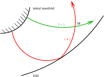
Figure 2.1: Initial manifold, rays & caustic

The geometrical amplitudes $A_{\pm}(\textbf{x})$ solve the transport equations $(\ref{transport})$, and according to $(\ref{amplitude})$ they are given by

$$A_{\pm}(\textbf{x})=\frac{\alpha_{0}(\theta_{\pm})}{\sqrt{J_{\pm}(\textbf{x})}}\ ,$$ (2.38)

where $\theta_{\pm}=\theta_{\pm}(\textbf{x})$ are the values of the parameter at the initial manifold corresponding to the rays $(\pm)$ passing from M, $\alpha_{0}(\theta_{\pm})$ are the corresponding initial amplitudes, and $J_{\pm}(\textbf{x})$ are the values of the Jacobian at the point x calculated along the $(\pm)$ rays. The value of the square root $\sqrt{J_{\pm}}$ is given by the formula $\sqrt{J_{\pm}}=\sqrt{\mid J_{\pm}\mid}e^{i{\frac{\pi}{2}}\gamma_{\pm}}$ where $\gamma_{+}=1$ and $\gamma_{-}=0$ . Note that $\gamma_{\pm}$ is the Maslov trajectory index, and it counts the number of tangencies of the rays with the caustic along their course from the points $\textbf{x}_{0}(\theta_{\pm})$ on the initial manifold to the point M. Moreover, the geometrical phases $S_{\pm}(\textbf{x})$ can be computed by integration along the rays according to $(\ref{gphase})$.

On the basis of the asymptotic formula $(\ref{klformula})$, Ludwig [Lu] has drawn the following qualitative picture of the wave field near the fold:

i) At points in the illuminated zone whose distance from the caustic is small compared with $\kappa^{-\frac{2}{3}}$, the predictions of geometrical optics are correct to order $-\frac{1}{2}$ .

ii) The intensity of the field on the caustic is large but finite (of order $\kappa^{\frac{1}{6}}$).

iii) In the shadow zone there is an illuminated strip (penumbra) of width of the order $\kappa^{\frac{2}{3}}$ . It must be emphasized here that WKB method fails to predict any penumbra as the shadow zone is devoid of classical rays.

It is finally interesting to note that we can construct the equations satisfied by functions $\phi$, $\rho$, $g_{0}$ and $g_{1}$ entering the Kravtsov-Kudwig formula $(\ref{klformula})$. For this, we substitute this formula into the Helmholtz equation $(\ref{helm})$, and we ask for the equation to be asymptotically valid for large $\kappa$. This procedure leads to the following system for the Kravtsov-Ludwig phases

$$\left(\nabla_{\bf{x}}\phi\right)^{2}+\rho\left(\nabla_{\bf{x}}\rho\right)^{2}=\eta^{2}(x)\ ,$$ (2.39)

$$\nabla_{\bf{x}}\phi\cdot\nabla_{\bf{x}}\rho=0\ .$$ (2.40)

The system for $g_{0}$, $g_{1}$ is rather complicated and it is given in [Lu], [KO].

2.4 Example: Plane wave incident on linear layer

We consider the two-dimensional Helmholtz equation

$$\Delta U(\textbf{x})+\kappa_{0}^{2}\eta^{2}(z)U(\textbf{x})=0\ ,\quad\textbf{x}=(y,z)$$

in a linearly stratified medium occupying the strip $0<z<h$, with refraction index (see Figure 2.2)

$$\eta^{2}(z)=\mu_{0}+\mu_{1}z$$

which increases with depth $z$ ($\mu_{1}>0$).

A plane wave of the form

$$U(y,h)=\exp(i\kappa_{0}y\sin{\psi})$$

arrives at the boundary $z=h$, with angle $\psi$ ($0<\psi<\pi/2$) with respect to the vertical direction $z$.

Figure 2.2: Caustic for a linear layer

For this medium, the Hamiltonian function is

$$H(y,z,k_{y},k_{z})=\frac{1}{2}\Bigl{(}|\textbf{k}|^{2}-\eta^{2}(z)\Bigr{)},\quad\textbf{k}=(k_{y},k_{z})$$

and the equations of the rays are given by the Hamiltonian system

$$\frac{dy}{dt} = k_{y}\ ,\quad y(0)=\xi$$

$$\frac{dz}{dt} = k_{z}\ ,\quad z(0)=h$$

$$\frac{dk_{y}}{dt} = 0\ ,\quad k_{y}(0)=\eta_{0}\sin{\psi}$$

$$\frac{dk_{z}}{dt} = -\frac{\mu_{1}}{2}\ ,\quad k_{z}(0)=-\eta_{0}\cos\psi\ .$$ (2.41)

Solving the above system, we find the parametric equations of the rays

$$z = \frac{\mu_{1}}{4}t^{2}-\eta_{0}t\cos{\psi}+h$$

$$y = \xi+\eta_{0}t\sin{\psi}\ .$$ (2.42)

The Jacobian of the ray transformation is given by

$$J=\frac{1}{\eta_{0}\cos{\psi}}\left|\matrix{\frac{\partial{y}}{\partial{t}}&\frac{\partial{z}}{\partial{t}}\cr\frac{\partial{y}}{\partial{\xi}}&\frac{\partial{z}}{\partial{\xi}}}\right|=\frac{1}{\eta_{0}\cos{\psi}}\Bigl{(}-\frac{\mu_{1}}{2}t+\eta_{0}\cos{\psi}\Bigr{)}\ ,$$ (2.43)

and it vanishes on the caustic given by

$$z_{c}=h-\frac{1}{\mu_{1}}{\eta_{0}}^{2}\cos^{2}{\psi}\ .$$ (2.44)

From the equations of the rays $(\ref{rays})$, and for any given point $(y,z<h)$, we find two values of the parameter $t$, that is

$$t_{+}(z) = \frac{2}{\mu_{1}}\Bigl{(}\eta_{0}\cos{\psi}+\sqrt{{\eta_{0}}^{2}\cos^{2}\psi+\mu_{1}(z-h)}\,\Bigr{)}\ ,$$ (2.45)

$$t_{-}(z) = \frac{2}{\mu_{1}}\Bigl{(}\eta_{0}\cos{\psi}-\sqrt{{\eta_{0}}^{2}\cos^{2}\psi+\mu_{1}(z-h)}\,\Bigr{)}\ ,$$ (2.46)

and the corresponding initial positions

$$\xi_{+}(y,z) = y-\frac{2}{\mu_{1}}\eta_{0}\sin{\psi}\Bigl{[}\eta_{0}\cos{\psi}+\sqrt{{\eta_{0}}^{2}\cos^{2}\psi+\mu_{1}(z-h)}\,\Bigr{]}\ ,$$ (2.47)

$$\xi_{-}(y,z) = y-\frac{2}{\mu_{1}}\eta_{0}\sin{\psi}\Bigl{[}\eta_{0}\cos{\psi}-\sqrt{{\eta_{0}}^{2}\cos^{2}\psi+\mu_{1}(z-h)}\,\Bigr{]}\ .$$ (2.48)

This means that from every given point $(y,z)$, at the times $t_{\pm}$ pass two rays emanating from the points $\xi_{\pm}$ on the illuminated boundary $z=h$. Note that for $z=z_{c}$ , we have $t_{+}(z_{c})=t_{-}(z_{c})=:t_{c}$ .

Using now the equation $(\ref{gphase})$ we compute the phase function

$$S(t) = \int_{0}^{t}\eta^{2}(z(\tau))d\tau+S(y(0),z(0))$$

$$= \int_{0}^{t}(\mu_{0}-\mu_{1}z(\tau))d\tau+S(\xi,h)$$

$$= \frac{{\mu_{1}}^{2}}{12}t^{3}-\frac{\mu_{1}\eta_{0}\cos\psi}{2}t^{2}+(\mu_{0}+\mu_{1}h)t+\eta_{0}\xi\sin{\psi}\ ,$$

and substituting the values of $t_{+}$ , $t_{-}$ , $\xi_{+}$ , $\xi_{-}$ , we obtain the geometrical phases

$$S_{+}(y,z) = -\frac{6(\mu_{0}+\mu_{1}h)(\alpha-\beta)+6\alpha^{2}\beta-4\alpha^{3}-2\beta^{3}}{3\mu_{1}}+\eta_{0}\xi_{+}\sin{\psi}\ ,$$ (2.49)

$$S_{-}(y,z) = -\frac{6(\mu_{0}+\mu_{1}h)(\alpha+\beta)-6\alpha^{2}\beta-4\alpha^{3}+2\beta^{3}}{3\mu_{1}}+\eta_{0}\xi_{-}\sin{\psi}$$ (2.50)

where

$$\alpha=-\eta_{0}\cos{\psi}\ ,\quad\beta=\sqrt{{\eta_{0}}^{2}\cos^{2}{\psi}+\mu_{1}(z-h)}\ .$$ (2.51)

Using the equations $(\ref{klphases})$, we compute the Kravtsov-Ludwig coordinates (modified phases)

$$\phi(y)=\frac{2}{3\mu_{1}}\eta_{0}^{3}\cos^{3}{\psi}+\eta_{0}y\sin{\psi}$$ (2.52)

and

$$\rho(z)={\Bigl{(}\frac{1}{\mu_{1}}\Bigr{)}}^{2/3}(\alpha^{2}+\mu_{1}(z-h))\ .$$ (2.53)

The Jacobians $J_{\pm}$ along the two rays passing from the point $(y,z)$, are given by

$$J_{+} = -\frac{1}{\eta_{0}\cos{\psi}}\sqrt{{\eta_{0}}^{2}\cos^{2}\psi+\mu_{1}(z-h)}\ ,$$ (2.54)

$$J_{-} = \frac{1}{\eta_{0}\cos{\psi}}\sqrt{{\eta_{0}}^{2}\cos^{2}\psi+\mu_{1}(z-h)}$$ (2.55)

and the corresponding principal geometrical amplitudes are

$$A_{+} = -i{(\eta_{0}\cos{\psi})}^{1/2}{\Bigl{[}\eta_{0}^{2}\cos^{2}{\psi}+\mu_{1}(z-h)\Bigr{]}}^{-1/4}\ ,$$ (2.56)

$$A_{-} = {(\eta_{0}\cos{\psi})}^{1/2}{\Bigl{[}\eta_{0}^{2}\cos^{2}{\psi}+\mu_{1}(z-h)\Bigr{]}}^{-1/4}\ .$$ (2.57)

Therefore the modified amplitudes $(\ref{modamplitudes})$ are given by

$$g_{0}=-i\sqrt{2}{(\eta_{0}\cos{\psi})}^{1/2}{\Bigl{(}\frac{1}{\mu_{1}}\Bigr{)}}^{1/6},\qquad g_{1}=0\ .$$ (2.58)

It is then easy to check that the Kravtsov-Ludwig formula coincides in the layer $0<z<h$ with the analytical solution of the Dirichlet boundary value problem in the half space $z<h$. In fact, by separation of variables we look for solutions of the form $U(y,z)=\exp(i\kappa_{0}y\sin\psi)\,u(z)$ , and it follows that $u(z)$ satisfies the ordinary equation $u^{\prime\prime}(z)+\kappa_{0}^{2}\bigl{(}\mu_{0}+\mu_{1}z-\sin^{2}\psi\bigr{)}\,u(z)=0$ which using the changes of variables $Z=\mu_{0}+\mu_{1}z-\sin^{2}\psi$ and $x=Z\epsilon^{1/3}\ ,\ \ \epsilon=(\mu_{1}/{\kappa_{0}})^{2}$ , is transformed to the Airy equation

$$\epsilon^{2}{{u^{\epsilon}}^{\prime\prime}(x)}+xu^{\epsilon}(x)=0\,,\quad x\in R\ .$$ (2.59)

In the sequel we are interested for the high-frequency regime, that is when $\epsilon$ is small, and we study as a model problem the geometrical optics of the semiclassical Airy equation $(\ref{sclairy})$.

2.5 Geometrical optics for the semiclassical Airy equation

According to the WKB method we are looking for asymptotic solution of the semiclassical Airy equation

$$\epsilon^{2}{{u^{\epsilon}}^{\prime\prime}(x)}+xu^{\epsilon}(x)=0\,,\quad x\in R$$

in the form

$$u^{\epsilon}(x)=A(x)\,e^{iS(x)/\epsilon}$$

where $S(x)$ is a real-valued phase and $A(x)$ is the complex-valued principal amplitude (from now on we drop the subscript in the principle amplitude $A_{0}$), solving the eikonal equation

$$(S^{\prime}(x))^{2}=x$$ (2.60)

and transport equation $(\ref{transport})$, respectively.

The Hamiltonian $(\ref{hamiltonian})$ is given by

$$H(x,k)=\frac{1}{2}\bigl{(}k^{2}-x\bigr{)}\ ,$$ (2.61)

and the corresponding Hamiltonian system $(\ref{hamsys})$ has the simple form

$$\frac{dx}{dt}=H_{k}=k\ ,\quad\frac{dk}{dt}=-H_{x}=\frac{1}{2}\ .$$ (2.62)

We assume that the rays are launched from a point source at $x=x_{0}$, where $x_{0}>0$, therefore $(\ref{hamsysairy})$ must satisfy the initial conditions

$$x(0)=x_{0}\ ,\quad k(0)=k_{0}\ .$$ (2.63)

Solving the system $(\ref{hamsysairy})$ with the above initial conditions we obtain the bicharacteristics

$$x(t;x_{0},k_{0})=t^{2}/4+k_{0}t+x_{0}\ ,\quad k(t;x_{0},k_{0})=t/2+k_{0}\ .$$ (2.64)

Now for constructing the rays, since $k_{0}$ must satisfy the condition $H(x_{0},k_{0})=0$, we have $k_{0}=\pm\,\sqrt{x_{0}}$ . The positive sign ($k_{0}=+\sqrt{x_{0}}$) corresponds to the ray

$$x_{R}(t;x_{0})=t^{2}/4+t\sqrt{x_{0}}+x_{0}$$ (2.65)

moving from $x_{0}$ towards $x=+\infty$ , while the negative one ($k_{0}=-\sqrt{x_{0}}$) to the ray

$$x_{L}(t;x_{0})=t^{2}/4-t\sqrt{x_{0}}+x_{0}$$ (2.66)

moving from $x_{0}$ towards the turning point $x=0$ (which is the caustic of the problem as we will see in the sequel).

The Jacobian of the right-moving ray $x_{R}$ is

$$J_{R}(t;x_{0})=\frac{\partial x_{R}}{\partial x_{0}}=1+t/2\sqrt{x_{0}}\ ,$$ (2.67)

and it is always positive. However, the Jacobian of the left-moving ray $x_{L}$ ,

$$J_{L}(t;x_{0})=\frac{\partial x_{L}}{\partial x_{0}}=1-t/2\sqrt{x_{0}}\ ,$$ (2.68)

vanishes for $t=t_{c}:=2\sqrt{x_{0}}$ corresponding to $x_{L}(t_{c};x_{0})=0$ . Therefore, $x=0$ is the caustic for the left-moving ray and it coincides with the turning point of the Airy equation.

We now observe that for any $x>x_{0}$ the equation $x_{R}(t;x_{0})=x$ has the single solution $t_{R}=2(\sqrt{x}-\sqrt{x_{0}})$ , while for $0<x<x_{0}$ the equation $x_{L}(t;x_{0})=x$ has two solutions

$$t_{-}=2(\sqrt{x_{0}}-\sqrt{x})\ ,\quad t_{+}=2(\sqrt{x_{0}}+\sqrt{x})\,$$ (2.69)

and the corresponding values of the Jacobian $J_{L}$ are

$$J_{-}=\frac{\sqrt{x}}{\sqrt{x_{0}}}>0\ ,\quad J_{+}=-\frac{\sqrt{x}}{\sqrt{x_{0}}}<0\ .$$ (2.70)

The arrival time $t_{-}$ and the Jacobian $J_{-}$ correspond to the ray left-moving ray from the source, while $t_{+}$ and $J_{+}$ correspond to the ray reflected from the caustic $x=0$ .

Moreover, using the formula $(\ref{gphase})$ and imposing the condition that the geometric phase of the rays emitted from the source must vanish at the source point (see Avila & Keller [AK] for a detailed analysis of the geometrical optics with point sources), we obtain the geometric phases

$$S_{\pm}(x)=\pm\frac{2}{3}x^{3/2}+\frac{2}{3}x_{0}^{3/2}\ ,\ \ 0<x<x_{0}\ ,$$ (2.71)

and

$$S_{R}(x)=\frac{2}{3}\bigl{(}\sqrt{x}-2\sqrt{x_{0}}\bigr{)}^{3}+\frac{2}{3}x_{0}^{3/2}\ ,\ \ x>x_{0}\ .$$ (2.72)

Note that $S_{R}(x_{0})=0$ , $S_{-}(x_{0})=0$ , that is the rays emitted by the source satisfy the Avila-Keller condition, while $S_{+}(x_{0})=\frac{4}{3}x_{0}^{3/2}$ for the reflected ray and $S_{+}(x=0)=S_{-}(x=0)=\frac{2}{3}x_{0}^{3/2}$ .

Concerning the geometry of the ray system, obviously the bicharacteristics $(\ref{airybich})$ lie on the Lagrangian manifold $\Lambda=\{(x,k):x=k^{2}\}$ since $k^{2}=(t/2+k_{0})^{2}=x+(k_{0}^{2}-x_{0})=x$ , and for $k=S_{\pm,R}^{\prime}(x)$ we have in fact $H(x,k)=0$ (see Figure 2.3).

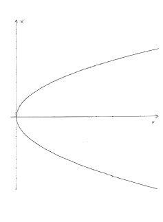
Figure 2.3: Lagrangian manifold for the semiclassical Airy equation

The principal amplitudes $A_{\pm}(x;x_{0})$ of the WKB waves along the rays in the region $0<x<x_{0}$ are found from $(\ref{amplitude})$ using the corresponding values of the Jacobian, and they are given by

$$A_{-}=\frac{\alpha_{0}}{\sqrt{J_{-}}}=\frac{\alpha_{0}x_{0}^{1/4}}{x^{1/4}}\ ,\quad A_{+}=\frac{\alpha_{0}}{\sqrt{J_{+}}}=-i\frac{\alpha_{0}x_{0}^{1/4}}{x^{1/4}}\ .$$ (2.73)

Then, the multiphase WKB solution in the region $0<x<x_{0}$ is given by

$$u^{\epsilon}_{WKB}(x) = A_{+}e^{iS_{+}(x)/\epsilon}+A_{-}e^{iS_{-}(x)/\epsilon}$$ (2.74)

$$= \alpha_{0}x_{0}^{1/4}e^{i\frac{1}{\epsilon}\frac{2}{3}x_{0}^{3/2}}\Bigl{(}-ix^{-1/4}e^{i\frac{1}{\epsilon}\frac{2}{3}x^{3/2}}+x^{-1/4}e^{-i\frac{1}{\epsilon}\frac{2}{3}x^{3/2}}\Bigr{)}\ .$$

Here $\alpha_{0}$ is the WKB amplitude of the wave at the source and it is equal to $\alpha_{0}=e^{-1/4}x_{0}^{-1/2}/2$ . This value follows from the asymptotics of the fundamental solution of the semiclassical Airy equation which are presented in Appendix A, in particular by comparing $(\ref{wkbairy})$ with (D.4). The same value would be derived by applying the Avila-Keller technique for the WKB approximation of fundamental solutions near the source point.

Finally the Kravtsov-Ludwig solution is found from the formula $(\ref{klformula})$. To apply this formula we compute the Kravtsov-Ludwig coordinates $(\ref{klphases})$ and the modified amplitudes $(\ref{modamplitudes})$,

$$\phi(x) = \frac{1}{2}\Bigl{(}S_{+}(x)+S_{-}(x)\Bigr{)}=\frac{2}{3}x_{0}^{3/2}$$ (2.75)

$$\rho(x) = \Biggl{[}\frac{3}{4}\biggl{(}S_{+}(x)+S_{-}(x)\biggr{)}\Biggr{]}^{2/3}=x$$ (2.76)

and

$$g_{0}(x) = \frac{1}{\sqrt{2}}\,\rho^{1/4}(x)\Bigl{(}A_{+}(x)-iA_{-}(x)\Bigr{)}=-\frac{1}{\sqrt{2}}\ e^{i\pi/4}x_{0}^{-1/4}$$ (2.77)

$$g_{1}(x) = \frac{1}{\sqrt{2}}\,\rho^{1/4}(x)\Bigl{(}A_{+}(x)+iA_{-}(x)\Bigr{)}=0\ .$$ (2.78)

Then the KL uniform solution in the region $0<x<x_{0}$ is given by

$$u^{\epsilon}_{KL}(x)=\pi^{1/2}e^{-i\pi/2}\Bigl{(}x_{0}^{-1/4}e^{i\frac{1}{\epsilon}\frac{2}{3}x_{0}^{3/2}}\Bigr{)}\epsilon^{-1/6}Ai\Biggl{(}-\frac{x}{\epsilon^{2/3}}\Biggr{)}$$ (2.79)

and it coincides with the fundamental solution (D) derived in Appendix D.

Chapter 3 Wigner functions and its asymptotics

3.1 The Wigner transform and basic properties

For any smooth complex valued function $\psi(x)$ rapidly decaying at infinity, say $\psi\in\mathcal{S}(R)$ , the Wigner transform of $\psi$ is a quadratic transform defined by

$$W[\psi](x,k)=W(x,k)=\frac{1}{2\pi}\int_{R}{e}^{-iky}\,\psi(x+\frac{y}{2})\,\overline{\psi}(x-\frac{y}{2})\,dy$$ (3.1)

where $\overline{\psi}$ is the complex conjugate of $\psi$. The Wigner transform is defined in phase space $R_{xk}$ , it is real, and it has, among others, the following remarkable properties.

First, the integral of $W(x,k)$ wrt. $k$ gives the squared amplitude (energy density) of $\psi$,

$$\int_{R}W(x,k)dk=|\psi(x)|^{2}\ .$$ (3.2)

In fact, we have

$$\int_{R}W(x,k)dk = \frac{1}{2\pi}\int_{R}\int_{R}e^{-iky}\,\psi(x+\frac{y}{2})\,\overline{\psi}(x-\frac{y}{2})\,dy\,dk$$ (3.3)

$$= \int_{R}\left(\frac{1}{2\pi}\int_{R}e^{-iky}\,dk\right)\psi(x+\frac{y}{2})\,\overline{\psi}(x-\frac{y}{2})\,dy$$

$$= \int_{R}\delta(y)\,\psi(x+\frac{y}{2})\,\overline{\psi}(x-\frac{y}{2})\,dy$$

$$= \psi(x)\,\overline{\psi}(x)=|\psi(x)|^{2}.$$

where we have used the Fourier transform $\delta(y)=\frac{1}{2\pi}\int_{R}e^{-iky}\,dk\,$ $\delta$ of Dirac’s measure.

Second, the first moment of $W(x,k)$ wrt. to $k$ gives the (energy) flux of $\psi$,

$$\int_{R}kW(x,k)\,dk=\frac{1}{2i}\Bigl{(}\psi(x)\,\overline{\psi^{{}^{\prime}}}(x)-\overline{\psi}(x)\,\psi^{{}^{\prime}}(x)\Bigr{)}={\mathcal{F}}(x)\ .$$ (3.4)

In fact, we have

$$\int_{R}kW(x,k)\,dk = \int_{R}\left(\frac{1}{2\pi}\int_{R}ke^{-iky}\,dk\right)\psi(x+\frac{y}{2})\,\overline{\psi}(x-\frac{y}{2})\,dy$$ (3.5)

$$= -\frac{1}{i}\int_{R}\delta^{{}^{\prime}}(y)\,\psi(x+\frac{y}{2})\,\overline{\psi}(x-\frac{y}{2})\,dy$$

$$= \frac{1}{i}\int_{R}\delta(y)\left(\frac{1}{2}\psi^{{}^{\prime}}(x+\frac{y}{2})\,\overline{\psi}(x-\frac{y}{2})-\frac{1}{2}\overline{\psi^{{}^{\prime}}}(x-\frac{y}{2})\,\psi(x+\frac{y}{2})\right)\,dy$$

$$= \frac{1}{2i}\left(\overline{\psi}(x)\,\psi^{{}^{\prime}}(x)-\psi(x)\,\overline{\psi^{{}^{\prime}}}(x)\right)\ .$$

The $x$ to $k$ duality in phase space can be recognized using the alternative definition

$$W(x,k)=\int_{R}e^{ipx}\,\widehat{\psi}(-k-\frac{p}{2})\,\overline{\widehat{\psi}}(-k+\frac{p}{2})\,dp\ ,$$ (3.6)

where $\widehat{\psi}(k)=\frac{1}{2\pi}\int_{R}e^{ikz}\,\psi(z)\,dz$ denotes the Fourier transform of $\psi$.

In fact, the definitions $(\ref{wig})$ and $(\ref{wigf})$ are equivalent, since we have

$$W(x,k) = \frac{1}{2\pi}\int_{R}e^{-iky}\,\psi(x+\frac{y}{2})\,\overline{\psi}(x-\frac{y}{2})\,dy$$ (3.7)

$$= \frac{1}{2\pi}\int_{R}e^{-iky}\int_{R}e^{-iz(x+\frac{y}{2})}\,\widehat{\psi}(z)\,dz\overline{\int_{R}e^{-iw(x-\frac{y}{2})}\,\widehat{\psi}(w)\,dw}\,dy$$

$$= \frac{1}{2\pi}\int_{R}e^{-iky}\int_{R}e^{-iz(x+\frac{y}{2})}\,\widehat{\psi}(z)\,dz\int_{R}e^{iw(x-\frac{y}{2})}\,\overline{\widehat{\psi}}(w)\,dw\,dy$$

$$= \int_{R}\int_{R}\left(\frac{1}{2\pi}\int_{R}e^{-iy(k+\frac{z}{2}+\frac{w}{2})}\,dy\right)e^{-i(z-w)x}\,\widehat{\psi}(z)\,\overline{\widehat{\psi}}(w)\,dz\,dw$$

$$= \int_{R}\int_{R}\delta(k+\frac{z}{2}+\frac{w}{2})\,e^{-i(z-w)x}\,\widehat{\psi}(z)\,\overline{\widehat{\psi}}(w)\,dz\,dw$$

$$= 2\int_{R}e^{-i2(k+z)x}\,\widehat{\psi}(z)\,\overline{\widehat{\psi}}(-2k-z)\,dz$$

$$= \int_{R}e^{ipx}\,\widehat{\psi}(-k-\frac{p}{2})\,\overline{\widehat{\psi}}(-k+\frac{p}{2})\,dp\ .$$

As we have explained in the previous chapter, in the case of high frequency wave propagation, it is useful to use WKB wave functions of the form

$$\psi^{\epsilon}(x)=A(x)\,e^{i{S(x)}/{\epsilon}}\ ,$$ (3.8)

where $S(x)$ is a real-valued and smooth phase, and $A(x)$ is a real-valued and smooth amplitude of compact support or at least rapidly decaying at infinity. The Wigner transform of $\psi^{\epsilon}(x)$ is the Wigner function

$$W(x,k):=W[\psi^{\epsilon}](x,k)=\frac{1}{2\pi}\int_{R}e^{-iky}\,e^{\frac{i}{\epsilon}S(x+\frac{y}{2})}\,A(x+\frac{y}{2})\,e^{-\frac{i}{\epsilon}S(x-\frac{y}{2})}\,\overline{A}(x-\frac{y}{2})\,dy\ ,$$ (3.9)

but $W(x,k)$ does not converge to a nontrivial limit, as $\epsilon\rightarrow 0$ . However, it can be shown that the rescaled version of $W(x,k)$ , that we call the scaled Wigner transform of $\psi^{\epsilon}$,

$$W^{\epsilon}(x,k)=\frac{1}{\epsilon}W\Bigl{(}x,\frac{k}{\epsilon}\Bigr{)}\$$ (3.10)

converges weakly as $\epsilon\rightarrow 0$ to the limit Wigner distribution [PR], [LP]

$$W^{0}(x,k)=|A(x)|^{2}\frac{1}{2\pi}\int_{R}e^{-i(k-S^{\prime}(x))y}\,dy=|A(x)|^{2}\delta(k-S^{\prime}(x))\ ,$$ (3.11)

which is a Dirac measure concentrated on the Lagrangian manifold $k=S^{\prime}(x)$ , associated with the phase of the WKB wavefunction, and it is the correct weak limit of $W^{\epsilon}$ (see, e.g., Lions & Paul [LP]).

Indeed, proceeding formally, we rewrite $W^{\epsilon}$ in the form

$$W^{\epsilon}(x,k)=\frac{1}{2\pi}\int_{R}e^{-iky}\,A(x+\frac{\epsilon y}{2})\,\overline{A}(x-\frac{\epsilon y}{2})\,e^{\frac{i}{\epsilon}\left[S(x+\frac{\epsilon y}{2})-S(x-\frac{\epsilon y}{2})\right]}\,dy\ ,$$

and we expand in Taylor series about $x$ both $A(x\pm\frac{\epsilon y}{2})$ and $S(x\pm\frac{\epsilon y}{2})$ . Then, we have

$$A(x+\frac{\epsilon y}{2})\,\overline{A}(x-\frac{\epsilon y}{2}) = \left(A(x)+\frac{\epsilon}{2}yA^{{}^{\prime}}(x)+\dots\right)\left(\overline{A}(x)-\frac{\epsilon}{2}y\overline{A}^{{}^{\prime}}(x)+\dots\right)$$

$$= A(x)\,\overline{A}(x)+O(\epsilon)$$

$$= |A(x)|^{2}+O(\epsilon)\ ,$$

and

$$S(x+\frac{\epsilon y}{2})-S(x-\frac{\epsilon y}{2}) = \left(S(x)+\frac{\epsilon}{2}yS^{{}^{\prime}}(x)+\frac{\epsilon^{2}}{8}y^{2}S^{{}^{\prime\prime}}(x)+\dots\right)$$

$$- \left(S(x)-\frac{\epsilon}{2}yS^{{}^{\prime}}(x)+\frac{\epsilon^{2}}{8}y^{2}S^{{}^{\prime\prime}}(x)-\dots\right)$$

$$= \epsilon yS^{{}^{\prime}}(x)+O(\epsilon^{3})\ .$$

Retaining only terms of order $O(1)$ in $A$ and $O(y)$ in $S$, and integrating the expansion termwise we obtain that $W^{\epsilon}(x,k)$ “converges” to $(\ref{diracwig})$.

More precisely, if $Q$ is any test function in $\mathcal{S}(R^{2}_{xk})$ , then

$$\int_{R}\int_{R}Q(x,k)\,W^{\epsilon}(x,k)\,dx\,dk\rightarrow\int_{R}Q(x,S^{{}^{\prime}}(x))\,|A(x)|^{2}dx\ .$$

The above observations suggest that the scaled Wigner transform

$$W^{\epsilon}(x,k) = \frac{1}{\epsilon}W\Bigl{(}x,\frac{k}{\epsilon}\Bigr{)}$$ (3.12)

$$= \frac{1}{2\pi}\int_{R}e^{-iky}\,\psi^{\epsilon}(x+\frac{\epsilon y}{2})\,\overline{\psi}^{\epsilon}(x-\frac{\epsilon y}{2})\,dy\ ,$$

is the correct phase-space object for analyzing high frequency waves.

3.2 Asymptotics of the Wigner function for a WKB wave function

Consider now the (scaled) Wigner function

$$W^{\epsilon}(x,k)=\frac{1}{\pi\epsilon}\int_{R}\ \psi^{\epsilon}(x+\sigma)\,\overline{\psi}^{\epsilon}(x-\sigma)\,\ e^{-\frac{i}{\epsilon}2k\sigma}\,d\sigma$$ (3.13)

of the WKB wave function

$$\psi^{\epsilon}(x)=A(x)\,e^{iS(x)/\epsilon}$$ (3.14)

where we assume that $A$, $S$ are smooth and real-valued, and $S^{\prime}(x)$ is globally concave.

We want to construct an asymptotic expansion of $W^{\epsilon}(x,k)$, that is the oscillatory integral

$$W^{\epsilon}(x,k)=\frac{1}{\pi\epsilon}\int_{R}D(\sigma,x)\,e^{i\frac{1}{\epsilon}F(\sigma,x,k)}\,d\sigma\ ,$$ (3.15)

where

$$D(\sigma,x)=A(x+\sigma)A(x-\sigma)$$ (3.16)

is the amplitude, and

$$F(\sigma,x,k)=S(x+\sigma)-S(x-\sigma)-2k\sigma$$ (3.17)

is the Wigner phase. Asymptotics of such integrals are usually constructed by applying the method of stationary phase.

For this purpose, we first compute the critical points of the phase $F(\sigma;x,k)$, that is the roots of

$$F_{\sigma}(\sigma;x,k)=S^{\prime}(x+\sigma)+S^{\prime}(x-\sigma)-2k=0$$ (3.18)

Figure 3.1: Berry’s chord

By the geometrical picture of Figure 3.1 (Berry’s chord construction; see the seminal paper by Berry [Ber]), we conclude that $(\ref{alpha})$ has a pair of symmetric roots $\pm\sigma_{0}(x,k)$ such that the point $P=(x,k)$ be the middle of a chord $QR$ having its ends on the Lagrangian (“manifold”) curve $\Lambda=\{k=S^{\prime}(x)\}$ .

We observe that as $P$ moves toward $\Lambda$ the chord $QR$ tends to the tangent of $\Lambda$ and $\sigma_{0}(x,k)\rightarrow 0$ . Therefore, the two critical points of $(\ref{alpha})$ tend to coalesce to the double point $\sigma=0$ as $P$ moves towards $\Lambda$.

In fact, we have

$$F_{\sigma\sigma}(\sigma,x,k)=S^{\prime\prime}(x+\sigma)-S^{\prime\prime}(x-\sigma)$$ (3.19)

and

$$F_{\sigma\sigma\sigma}(\sigma,x,k)=S^{\prime\prime\prime}(x+\sigma)+S^{\prime\prime\prime}(x-\sigma)$$ (3.20)

and therefore

$$F_{\sigma\sigma}(\sigma=0,x,k)=0\,,\quad F_{\sigma\sigma\sigma}(\sigma=0,x,k)=2S^{\prime\prime\prime}(x)\not=0$$ (3.21)

which assert that $\sigma=0$ is a double stationary point of $F$.

We would like therefore to apply a uniform stationary formula like that derived in Appendix C which holds even when the stationary points coalesce. For this we need to identify the parameter $\alpha$ of the uniform stationary formula, which controls the distance between the stationary points of the Wigner phase. In order to do this we expand F about $\sigma=0$ ,

$$F(\sigma;x,k) = S(x)+\sigma S^{\prime}(x)+\frac{\sigma^{2}}{2}S^{\prime\prime}(x)+\frac{\sigma^{3}}{6}S^{\prime\prime\prime}(x)+...$$

$$- \biggl{(}S(x)-\sigma S^{\prime}(x)+\frac{\sigma^{2}}{2}S^{\prime\prime}(x)-\frac{\sigma^{3}}{6}S^{\prime\prime\prime}(x)+...\biggr{)}-2k\sigma$$

$$= -2(k-S^{\prime}(x))\sigma+\frac{1}{3}S^{\prime\prime\prime}(x)\sigma^{3}+O(\sigma^{5})\ .$$

It becomes evident that for $P$ lying close enough to $\Lambda$, the parameter $\alpha$ has to be identified as

$$\alpha=\alpha(x,k):=k-S^{\prime}(x)\ .$$ (3.22)

Then, for any fixed $x$ we rewrite the Wigner phase $F$ in the form

$$F(\sigma;\alpha,x) = S(x+\sigma)-S(x-\sigma)-2\sigma(\alpha+S^{\prime}(x))$$ (3.23)

$$= \Bigl{(}S(x+\sigma)-S(x-\sigma)-2\sigma S^{\prime}(x)\Bigr{)}-2\sigma\alpha\ ,$$

and we have

$$F_{\sigma\sigma}(\sigma=0;x,k)=0\,,\quad F_{\sigma\sigma\sigma}(\sigma=0;x,k)=2S^{\prime\prime\prime}(x)\,,\quad F_{\sigma\alpha}(\sigma=0;\alpha,x)=-2\ .$$ (3.24)

These are exactly the conditions in Appendix C which are needed for applying the uniform asymptotic formula.

Then, the asymptotic formula of Appendix C ($B_{0}$ vanishes since $D$ is even wrt $\sigma$) gives the following approximation of the Wigner function

$$W^{\epsilon}(x,k)\approx 2\pi A_{0}(x,k){\epsilon}^{2/3}Ai\Bigl{(}-\epsilon^{2/3}\xi(x,k)\Bigr{)}$$ (3.25)

where

$$A_{0}(x,k)=2^{-1/2}\xi^{1/4}\frac{2D(\sigma_{o}(x,k),x)}{\mid F_{\sigma\sigma}(\sigma_{0}(x,k);x,k)\mid^{1/2}}\ ,$$ (3.26)

$$\xi(x,k)=\Biggl{[}\frac{3}{2}\Bigl{(}S(x+\sigma_{0})-S(x-\sigma_{0})-2k\sigma_{0}\Bigr{)}\Biggr{]}^{2/3}$$ (3.27)

and

$$F_{\sigma\sigma}(\sigma=\sigma_{0};x,k)=S^{\prime\prime}(x+\sigma_{0})-S^{\prime\prime}(x-\sigma_{0})<0\ .$$ (3.28)

We now further approximate the various quantities entering $(\ref{fullwigairy})$ as $\alpha\rightarrow 0$ . First of all, in this approximation

$$\xi \approx -F_{\sigma\alpha}\Biggl{(}\frac{F_{\sigma\sigma\sigma}}{2}\Biggr{)}^{-1/3}\alpha$$ (3.29)

$$= 2(k-S^{\prime}(x))\Biggl{(}\frac{2S^{\prime\prime\prime}(x)}{2}\Biggr{)}^{-1/3}$$

$$= 2(S^{\prime\prime\prime}(x))^{-1/3}(k-S^{\prime}(x))\ .$$

Furthermore we approximate

$$F_{\sigma\sigma}(\sigma=\sigma_{0};x,k)=S^{\prime\prime}(x+\sigma_{0})-S^{\prime\prime}(x-\sigma_{0})\approx 2\sigma_{0}(x,k)S^{\prime\prime\prime}(x)$$ (3.30)

and since $\sigma_{0}$ is approximated by

$$\sigma_{0} \approx (-2F_{\sigma\sigma\sigma}\ F_{\sigma\alpha}\ \alpha)^{1/2}(F_{\sigma\sigma\sigma})^{-1}$$ (3.31)

$$= (-2\cdot 2S^{\prime\prime\prime}(x)(-2)(k-S^{\prime}(x))^{1/2}(2S^{\prime\prime\prime}(x))^{-1}$$

$$= \Biggl{(}\ \frac{2}{S^{\prime\prime\prime}(x)}(k-S^{\prime}(x))\ \Biggr{)}^{1/2}$$

when $\alpha\rightarrow 0$ , we have

$$F_{\sigma\sigma}(\sigma_{0},x,k)\approx 2\sigma_{0}S^{\prime\prime\prime}(x)=2\Biggl{[}\ \frac{2(k-S^{\prime}(x))}{S^{\prime\prime\prime}(x)}\ \Biggr{]}^{1/2}S^{\prime\prime\prime}(x)\ ,$$ (3.32)

and then

$$\frac{\xi^{1/4}}{\mid F_{\sigma\sigma}\mid^{1/2}}=\Biggl{(}\frac{2}{\mid S^{\prime\prime\prime}(x)\mid}\Biggr{)}^{1/3}\frac{1}{2^{1/2+1/3}}\quad.$$ (3.33)

Moreover, since $D(\sigma_{o};x)=D(-\sigma_{0};x)$ , it follows

$$B_{0}=0$$ (3.34)

and using the approximation $(\ref{zeta})$ of $\xi$, we have

$$A_{0}=\frac{1}{2^{1/3}}\Biggl{(}\frac{2}{\mid S^{\prime\prime\prime}(x)\mid}\Biggr{)}^{1/3}D(\sigma_{0}(x,k),x)\ .$$ (3.35)

Finally, using $(\ref{fullwigairy})$ with

$$F(\sigma=0;x,k)=0\ ,\quad B_{0}=0$$

and $\xi$, $A_{0}$ given by ${(\ref{zeta})}$, ${(\ref{delta})}$, respectively, we arrive to the Airy-type approximation of ${(\ref{wigwkb})}$,

$$\widetilde{W}^{\epsilon}(x,k) \approx \frac{2^{2/3}}{\epsilon^{2/3}}\Biggl{(}\frac{2}{\mid S^{\prime\prime\prime}(x)\mid}\Biggr{)}^{1/3}D(\sigma_{o}(x,k),x)\cdot$$ (3.36)

$$\cdot Ai\Biggl{(}-\frac{2^{2/3}}{\epsilon^{2/3}}\Biggl{(}\frac{2}{\mid S^{\prime\prime\prime}(x)\mid}\Biggr{)}^{1/3}(k-S^{\prime}(x))\Biggr{)}$$

which is Berry’s semiclassical approximation of $W^{\epsilon}$, and we call it the semiclassical Wigner function (of the WKB function). Note that $(\ref{sclwigairy})$ is an approximation of $(\ref{fullwigairy})$ which holds locally near the manifold ($\alpha=k-S^{\prime}(x)$ very small).

Chapter 4 Wignerization of two-phase WKB solutions

In this chapter we study the structure of the Wigner transform of wave functions whose high-frequency asymptotics are described by two-phase WKB solutions, which is typical for wave fields around fold caustics. In order to start understanding the related asymptotic mechanisms, we first investigate the Wigner transform of the Airy function and its relation to the Wigner transform of the WKB asymptotic solution of the semiclassical Airy equation.

More precisely, we first compute the exact Wigner transform $W^{\epsilon}_{Ai}$ (see $(\ref{wigfundairy})$ below) of the fundamental solution

$$u^{\epsilon}(x)=\pi^{1/2}e^{-i\pi/2}\Bigl{(}x_{0}^{-1/4}e^{i\frac{1}{\epsilon}\frac{2}{3}x_{0}^{3/2}}\Bigr{)}\epsilon^{-1/6}Ai\left(-\epsilon^{-2/3}x\right)\ ,$$

(cf eq. $(\ref{innerairy})$) of the semiclassical Airy equation. Recall that the Kravtsov-Ludwig formula $(\ref{klairy})$ coincides with $(\ref{fundairy})$ in this case.

In the sequel we compute the asymptotics of the Wigner transform of the WKB approximation $(\ref{wkbairy})$ of the fundamental solution, using the semiclassical Wigner function developed in previous chapter, and we show that this approximation coincides with the exact Wigner transform $(\ref{wigfundairy})$ below.

4.1 Wigner transform of the Airy function

We start with the integral representation

$$\psi^{\epsilon}(x):=Ai(-\epsilon^{-2/3}x)=\frac{1}{2\pi}\int_{R}e^{i(\frac{\rho^{3}}{3}-\epsilon^{-2/3}x\rho)}\,d\rho\ ,$$ (4.1)

of the Airy function. The scaled Wigner transform $W^{\epsilon}$ of $\psi^{\epsilon}$ is given by

$$W^{\epsilon}[\psi^{\epsilon}](x,k)=\frac{1}{\pi\epsilon}\int_{R}\ \psi^{\epsilon}(x+\sigma)\,\overline{\psi}^{\epsilon}(x-\sigma)\,e^{-\frac{i}{\epsilon}2k\sigma}\,d\sigma\,$$ (4.2)

and therefore, if we substitute $(\ref{airy})$ and we put $\lambda=\epsilon^{-2/3}$, we have

$$W^{\epsilon}[\psi^{\epsilon}](x,k) = (2\pi)^{-3}\int_{R}\int_{R}e^{i\frac{1}{3}(\rho^{3}-\sigma^{3})}\,e^{-i\lambda x(\rho-\sigma)}\int_{R}e^{-i\left(k+\lambda\epsilon(\rho+\sigma)/2\right)\tau}\,d\tau\,d\rho\,d\sigma$$

$$= (2\pi)^{-2}\,2\epsilon^{-1/3}\int_{R}\int_{R}e^{i\frac{1}{3}(\rho^{3}-\sigma^{3})}\,e^{-i\lambda x(\rho-\sigma)}\,\delta\left(\rho+\sigma+2k\epsilon^{-1/3}\right)\,d\rho\,d\sigma\ ,$$

where Dirac’s mass is expressed through the Fourier transform

$$\delta(z)=\frac{1}{2\pi}\int_{R}e^{-iz\tau}\,d\tau\ .$$ (4.3)

On the support of Dirac’s mass $\sigma=-(\rho+2\epsilon^{-1/3}k)$, and $\rho-\sigma=2(\rho+u)$ with $u=\epsilon^{-1/3}k$ , so we have

$$\rho^{3}-\sigma^{3}=2\rho^{3}+6u\rho^{2}+12u^{2}\rho+8u^{3}\ .$$

After some straightforward algebra, and by the linear change $\rho=2^{-1/3}r-u$ , we obtain

$$W^{\epsilon}[\psi^{\epsilon}](x,k)=\frac{2^{2/3}}{2\pi}\,\epsilon^{-1/3}\int_{R}e^{i\Bigl{(}\frac{\tau^{3}}{3}+2^{-1/3}\left(2u^{2}-2\lambda x\right)\tau\Bigr{)}}\,d\tau\ ,$$ (4.4)

which by the integral representation (4.1) gives the Wigner transform of the Airy function

$$W^{\epsilon}[\psi^{\epsilon}](x,k)=\frac{1}{2^{1/3}\epsilon^{1/3}\pi}\,Ai\Bigl{(}2^{2/3}\epsilon^{-2/3}(k^{2}-x)\Bigr{)}\ .$$ (4.5)

Then, the Wigner transform of the fundamental solution $(\ref{fundairy})$ is given by

$$W^{\epsilon}_{Ai}(x,k):=W^{\epsilon}[u^{\epsilon}](x,k)=\frac{1}{2^{1/3}\epsilon^{2/3}}\,x_{0}^{-1/2}Ai\Bigl{(}2^{2/3}\epsilon^{-2/3}(k^{2}-x)\Bigr{)}\ .$$ (4.6)

By employing the asympotics of the Airy function we see that in the interior of the Lagrangian manifold $x>k^{2}$, $W^{\epsilon}[u^{\epsilon}]$ oscillates at the scale $\epsilon$,

$$W^{\epsilon}[u^{\epsilon}](x,k)\approx\frac{1}{\sqrt{2\pi}}\ \epsilon^{-1/2}x_{0}^{-1/2}{(x-k^{2})}^{-1/4}\cos{\Biggl{(}\frac{4}{3\epsilon}(x-k^{2})^{3/2}-\frac{\pi}{4}\Biggr{)}}\ ,$$ (4.7)

while at the exterior of the manifold (which is connected to the shadow region) $x<k^{2}$, $W^{\epsilon}[u^{\epsilon}]$ decays exponentially

$$W^{\epsilon}[u^{\epsilon}](x,k)\approx\frac{1}{2^{3/2}\sqrt{\pi}}\ \epsilon^{-1/2}x_{0}^{-1/2}{(k^{2}-x)}^{-1/4}e^{-\frac{4}{3\epsilon}(k^{2}-x)^{3/2}}\ .$$ (4.8)

This asymptotic picture suggests the existence of a transition boundary layer with thickness $O(\epsilon^{2/3})$ around the Lagrangian manifold $x=k^{2}$ , inside which the wave field is described by Airy structure and where most of the energy of the wave field is concentrated.

The weak limit of $W^{\epsilon}[u^{\epsilon}]$ as $\epsilon\rightarrow 0$ , is computed by the formula

$$\frac{1}{\epsilon}F\left(\frac{z}{\epsilon}\right)\ \rightarrow\delta(z)\int_{R}F(y)\,dy\ ,\ \ \epsilon\rightarrow 0\ ,$$ (4.9)

and, since

$$\int_{R}Ai(y)dy=1\ ,$$

it is given by

$$W^{0}(x,k)=x_{0}^{-1/2}2^{-1/3}\delta\left(2^{2/3}(k^{2}-x)\right)=\frac{1}{2x_{0}^{1/2}}\,\delta(k^{2}-x)\ .$$ (4.10)

Note that in the illuminated zone $x>0$ ,

$$W^{0}(x,k)=\frac{1}{2x_{0}^{1/2}}\,\delta(k^{2}-x)=\frac{1}{4x_{0}^{1/2}x^{1/2}}\Bigl{(}\delta(k-x^{1/2})+\delta(k+x^{1/2})\Bigr{)}\ ,$$ (4.11)

that is, $W^{0}$ splits to two Dirac masses supported on the branches $k=\pm\,x^{1/2}$ . This splitting fails on the caustic $x=0$ , while in the shadow zone $x<0$ the limit Wigner $W^{0}$ is weakly zero since $k^{2}-x>0$ .

On the other hand we can compute the limit Wigner distribution of the (two-phase) WKB expansion of the fundamental solution $(\ref{wkbairy})$ of the semiclassical Airy equation (cf also (D.4)),

$$u^{\epsilon}_{WKB}(x) = A_{+}(x)\,e^{iS_{+}(x)/\epsilon}+A_{-}(x)\,e^{iS_{-}(x)/\epsilon}$$

$$= \alpha_{0}x_{0}^{1/4}\,e^{i\frac{1}{\epsilon}\frac{2}{3}x_{0}^{3/2}}\Bigl{(}-ix^{-1/4}e^{i\frac{1}{\epsilon}\frac{2}{3}x^{3/2}}+x^{-1/4}\,e^{-i\frac{1}{\epsilon}\frac{2}{3}x^{3/2}}\Bigr{)}\ ,$$

By $(\ref{diracwig})$ we have the weak limits

$$W^{\epsilon}\Biggl{[}A_{\pm}(x)e^{iS_{\pm}(x)/\epsilon}\Biggr{]}\ \rightarrow\ {\mid A_{\pm}(x)\mid}^{2}\delta(k-S^{\prime}_{\pm}(x))\ ,\quad\epsilon\rightarrow 0\ .$$

Moreover, the cross Wigner transform

$$W^{\epsilon}\biggl{[}A_{+}(x)\,e^{iS_{+}(x)},A_{-}(x)\,e^{iS_{-}(x)}\biggr{]}=$$

$$=(\pi\epsilon)^{-1}\int_{R}A_{+}(x+\sigma)\,\overline{A}_{-}(x-\sigma)\,e^{i\frac{1}{\epsilon}\bigl{(}S_{+}(x+\sigma)-S_{+}(x-\sigma)-2k\sigma\bigr{)}}\,d\sigma\ ,$$ (4.12)

converges weakly to zero, since following the same reasoning as for proving $(\ref{diracwig})$ by expanding the phase and the amplitude in Taylor series wrt. $\sigma$, we get in front of the integral the oscillatory term

$$e^{i{\frac{1}{\epsilon}}\bigl{(}S_{\pm}(x)-S_{\mp}(x)\bigr{)}}\ ,$$

which weakly tends to zero as $\epsilon\rightarrow 0$, for $S^{\prime}_{+}(x)\neq-S^{\prime}_{-}(x)$ .

It then follow that

$$W^{\epsilon}[u^{\epsilon}_{WKB}](x,k)\ \rightarrow{\mid A_{+}(x)\mid}^{2}\delta(k-S^{\prime}_{+}(x))+{\mid A_{-}(x)\mid}^{2}\delta(k-S^{\prime}_{-}(x))$$

$$=\frac{1}{4x_{0}^{1/2}x^{1/2}}\biggl{(}\delta(k-x^{1/2})+\delta(k+x^{1/2})\biggr{)}\ ,$$ (4.13)

and, as it is anticipated for $\epsilon\rightarrow 0$ , we derive that

$$W^{\epsilon}[u^{\epsilon}_{WKB}](x,k)\rightarrow W^{0}(x,k)\ .$$ (4.14)

4.2 Wigner transform of the WKB expansion for the Airy equation

We have already constructed the WKB solution of the Airy equation in the form

$$u^{\epsilon}_{WKB}(x)=A_{+}(x)\,e^{\frac{i}{\epsilon}S_{+}(x)}+A_{-}(x)\,e^{\frac{i}{\epsilon}S_{-}(x)}\ ,$$ (4.15)

where the phases $S_{\pm}$ and the amplitudes $A_{\pm}$ are given by $(\ref{airyphases})$ and $(\ref{arrampl})$,

$$S_{\pm}(x)=\pm\frac{2}{3}x^{3/2}+\frac{2}{3}{x_{0}}^{3/2}\ ,$$

and

$$A_{+}(x)=(-i)\frac{1}{2}x^{-1/4}e^{-i\pi/4}{x_{0}}^{-1/4}\ ,\ \ A_{-}(x)=\frac{1}{2}x^{-1/4}e^{-i\pi/4}{x_{0}}^{-1/4}\ .$$

The scaled Wigner transform of $u^{\epsilon}_{WKB}$ is given by

$$W_{WKB}^{\epsilon}(x,k)=\frac{1}{\pi\epsilon}\sum_{\ell=1}^{4}\int_{R}{}D_{\ell}(\sigma;x)\ e^{\frac{i}{\epsilon}F_{\ell}(\sigma;x,k)}\,d\sigma=\sum_{\ell=1}^{4}W^{\epsilon}_{\ell}(x,k)$$ (4.16)

where

$$W^{\epsilon}_{\ell}(x,k)=\int_{R}D_{\ell}(\sigma;x)\,e^{\frac{i}{\epsilon}F_{\ell}(\sigma;x,k)}\,d\sigma\,,\quad\ell=1,..,4\ .$$ (4.17)

The amplitudes and phases of the above four Wigner integrals are given by

$$D_{1}(\sigma;x) = A_{+}(x+\sigma)\overline{A}_{+}(x-\sigma)$$

$$D_{2}(\sigma;x) = A_{-}(x+\sigma)\overline{A}_{-}(x-\sigma)$$

$$D_{3}(\sigma;x) = A_{+}(x+\sigma)\overline{A}_{-}(x-\sigma)$$

$$D_{4}(\sigma;x) = A_{-}(x+\sigma)\overline{A}_{+}(x-\sigma)$$ (4.18)

and

$$F_{1}(\sigma;x,k) = S_{+}(x+\sigma)-S_{+}(x-\sigma)-2k\sigma$$ (4.19)

$$F_{2}(\sigma;x,k) = S_{-}(x+\sigma)-S_{-}(x-\sigma)-2k\sigma$$ (4.20)

$$F_{3}(\sigma;x,k) = S_{+}(x+\sigma)-S_{-}(x-\sigma)-2k\sigma$$ (4.21)

$$F_{4}(\sigma;x,k) = S_{-}(x+\sigma)-S_{+}(x-\sigma)-2k\sigma\ .$$ (4.22)

In the sequel we compute the stationary-phase asymptotic expansions of the Wigner integrals $W^{\epsilon}_{\ell}$ , using either the standard or the uniform formula according to the structure of the stationary points in each case.

4.2.1 Stationary points of the Wigner phases

In the sequel we compute the stationary points of the Wigner phases in the illuminated area $x>0$ , since the real-valued phases $S_{\pm}(x)$ of the WKB solution have been computed only in the illuminated region. It turns out that all real stationary points, which give the main asymptotic contribution to the Wigner integrals, lie in the area $|\sigma|<x$ in which the Wigner phases are real. Outside this area, the stationary points are imaginary and their contribution to the Wigner integrals is exponentially small.

Stationary points of the Wigner phase $F_{1}(\sigma;x,k)$ . The critical points of $F_{1}(\sigma;x,k)$ are given by

$${F_{1}}_{\sigma}(\sigma;x,k)=S_{+}^{\prime}(x+\sigma)+S_{+}^{\prime}(x-\sigma)-2k=0\ ,$$ (4.23)

that is

$$(x+\sigma)^{1/2}+(x-\sigma)^{1/2}-2k=0\ .$$ (4.24)

For $k<0$ we see that the phase $F_{1}(\sigma;x,k)$ has not critical points since $(x\pm\sigma)^{1/2}>0$ , while for $k>0$ we can see that the roots of $(\ref{symeq})$ appear in symmetric pairs. In fact, if we set $\sigma=\sigma_{R}+i\sigma_{I}$ and substitute into (4.24) we have

$$(\sigma_{R}-2k^{2})^{2}-{\sigma_{I}}^{2}+2i\sigma_{I}(\sigma_{R}-2k^{2})=4k^{2}(x-\sigma_{R})-4k^{2}\sigma_{I}i\ ,$$ (4.25)

and equating the real and imaginary parts to zero, we obtain

$$(\sigma_{R}-2k^{2})^{2}-{\sigma_{I}}^{2}-4k^{2}(x-\sigma_{R})=0$$ (4.26)

$$\sigma_{I}\sigma_{R}=0\ .$$ (4.27)

Thus we must consider the following cases.

Case 1 : $\sigma_{I}=0$ . Then, $\sigma=\sigma_{R}\in R$ and $(\ref{stsya})$ gives

$$(x^{2}-\sigma^{2})^{1/2}=2k^{2}-x\ ,$$ (4.28)

which implies the restriction $x\leq 2k^{2}$ . From the last equation we find that the real critical points of $F_{1}$ are

$$\sigma(x,k)=\pm 2|k|(x-k^{2})^{1/2}=:\pm\sigma_{0}(x,k)\ .$$ (4.29)

Therefore, in the region $k^{2}<x\leq 2k^{2}$ $F_{1}$ has two real stationary points, the $\pm\sigma_{0}(x,k)=\pm 2|k|(x-k^{2})^{1/2}$ , which coalesce to $\sigma(x,k)=0$ on the upper branch of the Lagrangian manifold $x=k^{2}$ . Now since

$${F_{1}}_{\sigma\sigma}(\sigma=\pm\sigma_{0};x,k)=\frac{1}{2}\frac{(x\mp\sigma_{0})^{1/2}-(x\pm\sigma_{0})^{1/2}}{(x^{2}-\sigma_{0}^{2})^{1/2}}\not=0\ ,$$ (4.30)

and

$${F_{1}}_{\sigma\sigma}(\sigma=0;x,k)=0\ ,\quad{F_{1}}_{\sigma\sigma\sigma}(\sigma=0;x,k)=-\frac{1}{2}x^{-3/2}\not=0\ ,$$ (4.31)

it turns out that the points $\pm\sigma_{0}(x,k)$ are simple and the point $\sigma(x,k)=0$ formatted by the coalescence of $\pm\sigma_{0}(x,k)$ is double. In fact, by Berry’s chord construction we see that, as we move toward the Lagrangian manifold $\{(x,k):k=S_{+}^{\prime}(x)\}$ the chord tends to the tangent of the manifold, and the critical points $\pm\sigma_{0}$ tend to the double stationary point $\sigma=0$ .

Case 2 : $\sigma_{I}\not=0$ . Then from (4.27) we have

$$\sigma_{I}=\pm 2|k|(k^{2}-x)^{1/2}\ ,$$

and therefore for $x<k^{2}$ $F_{1}$ has simple imaginary stationary points $\sigma(x,k)=\pm 2|k|i(k^{2}-x)^{1/2}$ , since in this region

$${F_{1}}_{\sigma\sigma}(\sigma=\pm i\sigma_{0};x,k)\not=0\ .$$

Stationary points of the Wigner phase $F_{2}(\sigma;x,k)$ . The critical points of $F_{2}$ are given by the equation

$${F_{2}}_{\sigma}(\sigma;x,k)=S_{-}^{\prime}(x+\sigma)+S_{-}^{\prime}(x-\sigma)-2k=0$$

that is,

$$(x+\sigma)^{1/2}+(x-\sigma)^{1/2}+2k=0\ .$$ (4.32)

For $k>0$ the equation (4.32) has no solution since $(x\pm\sigma)^{1/2}>0$ . For $k<0$ we set $\sigma=\sigma_{R}+i\sigma_{I}$ into (4.32) and we obtain again the system (4.26), $(\ref{stsyb})$ . Therefore, the critical points of $F_{2}$ are $\sigma(x,k)=\pm 2|k|(x-k^{2})^{1/2}=\pm\sigma_{0}$ , when $k^{2}\leq x\leq 2k^{2}$ and $\sigma(x,k)=\pm 2|k|i(k^{2}-x)^{1/2}=\pm i\sigma_{0}$ , when $x<k^{2}$ .

At any point $(x,k)$ in $k^{2}<x\leq 2k^{2}$ there exist two simple stationary points, $\pm\sigma_{0}$. For fixed $(x,k)$ moving towards $S_{-}^{\prime}(x)=-\sqrt{x}$ we see again that the critical points coalesce to the double point $\sigma=0$ . Finally, in the region $x<k^{2}$ we have two simple imaginary stationary points, $\pm i\sigma_{0}$ , which again coalesce to $\sigma=0$ on the lower branch of the Lagrangian manifold $x=k^{2}$ .

Stationary points of the Wigner phase $F_{3}(\sigma;x,k)$ . The critical points of the phase $F_{3}(\sigma;x,k)$ are given by the equation

$$(x+\sigma)^{1/2}-(x-\sigma)^{1/2}-2k=0\ .$$ (4.33)

In this case we find that the solutions of the above equation are $\sigma=\pm 2|k|(x-k^{2})^{1/2}=\pm\sigma_{0}$ for $x\geq 2k^{2}$ , and $\sigma=\pm 2|k|i(k^{2}-x)^{1/2}=\pm i\sigma_{0}$ for $x<k^{2}$ . By geometrical considerations similar to Berry’s chord construction, we see that for fixed $(x,k)$ with $x>2k^{2}$ , the stationary point is $\sigma=+\sigma_{0}$ if $k>0$, while if $k<0$ the stationary point is $\sigma=-\sigma_{0}$ . These stationary points are always simple since

$${F_{3}}_{\sigma\sigma}(\sigma=\pm\sigma_{0};x,k)=\frac{1}{2}\frac{(x\mp\sigma_{0})^{1/2}+(x\pm\sigma_{0})^{1/2}}{(x^{2}-\sigma_{0}^{2})^{1/2}}\not=0\ ,$$ (4.34)

and

$${F_{3}}_{\sigma\sigma}(\sigma=\pm i\sigma_{0};x,k)=\frac{1}{2}\frac{(x\mp i\sigma_{0})^{1/2}+(x\pm i\sigma_{0})^{1/2}}{(x^{2}+\sigma_{0}^{2})^{1/2}}\not=0\ .$$ (4.35)

Note that ${F_{3}}_{\sigma\sigma}(\sigma=\pm\sigma_{0};x,k)$ becomes infinite for $x=2k^{2}$ .

Finally, it is important to observe that in this case there are no stationary points in the region $k^{2}<x<2k^{2}$ .

Stationary points of the Wigner phase $F_{4}(\sigma;x,k)$ . In this case the critical points are $\sigma=\pm\sigma_{0}$ when $x\geq 2k^{2}$ and $\sigma=\pm i\sigma_{0}$ when $x<k^{2}$ . Here, for fixed $x$ with $x>2k^{2}$ , the stationary point is $\sigma=-\sigma_{0}$ for $k>0$ , and $\sigma=+\sigma_{0}$ for $k<0$ . Again, the stationary points $\pm\sigma_{0}$ and $\pm i\sigma_{0}$ are simple.

For easier consideration of the structure of the stationary points, the results of the above computations are tabulated in the following two tables, where we have set $\sigma_{0}=\sigma_{0}(x,k)=2\ |k|\mid x-k^{2}\mid^{1/2}$ .

$F_{i},k$	$(-\infty,-\sqrt{x})$	$(-\sqrt{x},-\sqrt{x/2})$	$(-\sqrt{x/2},\sqrt{x/2})$	$(\sqrt{x/2},\sqrt{x})$	$(\sqrt{x},\infty)$
$F_{1}$	no s.p.	no s.p.	no s.p.	$\sigma=\pm\sigma_{0}$	$\sigma=\pm i\sigma_{0}$
				simples	simples
$F_{2}$	$\sigma=\pm i\sigma_{0}$	$\sigma=\pm\sigma_{0}$	no s.p.	no s.p.	no s.p.
	simples	simples
$F_{3}$	$\sigma=\pm i\sigma_{0}$	no s.p.	$\sigma=\pm\sigma_{0}$	no s.p.	$\sigma=\pm i\sigma_{0}$
	simples		simple		simples
$F_{4}$	$\sigma=\pm i\sigma_{0}$	no s.p.	$\sigma=\pm\sigma_{0}$	no s.p.	$\sigma=\pm i\sigma_{0}$
	simples		simple		simples

Table 4.1: A. Stationary points between the parabolas

$F_{i},k$	$k=-\sqrt{x}$	$k=-\sqrt{x/2}$	$k=\sqrt{x/2}$	$k=\sqrt{x}$
$F_{1}$	no s.p.	no s.p.	$\sigma=\pm\sigma_{0}$	$\sigma=0$
			simples	double
$F_{2}$	$\sigma=0$	$\sigma=\pm\sigma_{0}$	no s.p.	no s.p.
	double	simples
$F_{3}$	no s.p.	$\sigma=-\sigma_{0}$	$\sigma=+\sigma_{0}$	no s.p.
		simple	simple
$F_{4}$	no s.p.	$\sigma=+\sigma_{0}$	$\sigma=-\sigma_{0}$	no s.p.
		simple	simple

Table 4.2: B. Stationary points on the parabolas

4.2.2 Asymptotics of the diagonal Wigner function

For constructing the asymptotics of the diagonal Wigner functions $W_{1}^{\epsilon}$ , $W_{2}^{\epsilon}$ , we first observe that the asymptotic contribution to $W_{1}^{\epsilon}$ comes from the stationary points in the region $x\leq 2k^{2}$ , $k>0$ , while the contribution to $W_{2}^{\epsilon}$ comes from the stationary points in the region $x\leq 2k^{2}$ , $k<0$ , since there are no stationary point of the corresponding Wigner phases outside from the above indicated regions, respectively.
We therefore consider the following two regions.

Region 1 : $k^{2}\leq x\leq 2k^{2}$

Because $\sigma=0$ is a double stationary point for the diagonal Wigner phases on the Lagrangian manifold $x=k^{2}$ (see Tables 4.1, 4.2) we need to apply the uniform approximation formula $(\ref{fullwigairy})$ of Section 3.2. .

For the integral $W_{1}^{\epsilon}(x,k)$ we choose the parameter $\alpha=\alpha(x,k):=k-\sqrt{x}$ . Expanding $F_{1}$ in Taylor series about $\sigma=0$ , we have

$${F_{1}}(\sigma;\alpha,x)=-2\alpha\sigma-\frac{1}{12}x^{-3/2}\sigma^{3}$$ (4.36)

and ${F_{1}}_{\sigma\alpha}(\sigma=0,\alpha=0,x)=-2\neq 0$ , and we easily see that all other conditions for the validity of $(\ref{fullwigairy})$ also hold. For applying this formula, we need to compute the unknowns $\xi$, $A_{0}$, $B_{0}$, and $F_{1}(\sigma=0,\alpha=0,x)$ .

From $(\ref{fullzeta})$ we have

$$\xi(x,k)=\Biggl{[}\frac{3}{4}\biggl{(}F_{1}(\sigma_{0})-F_{1}(-\sigma_{0})\biggr{)}\Biggr{]}^{2/3}=\Biggl{[}\frac{3}{4}\biggl{(}4\frac{2}{3}(x-k^{2})^{3/2}\biggr{)}\Biggr{]}^{2/3}=2^{2/3}(x-k^{2})\ ,$$

and from (3.26) we get

$$A_{0}=2^{7/6}(x-k^{2})^{1/4}(x^{2}-{\sigma_{0}}^{2})^{-1/4}x^{3/4}{x_{0}}^{-1/2}{\sigma_{0}}^{-1/2}\ .$$

Since $(x^{2}-{\sigma_{0}}^{2})^{1/2}=2k^{2}-x$ , we rewrite $A_{0}$ in the form

$$A_{0}=2^{-4/3}k^{-1/2}x^{3/4}{x_{0}}^{-1/2}(2k^{2}-x)^{-1/2}\ .$$ (4.37)

and from $(\ref{taylorF1})$ we also have $F_{1}(\sigma=0,\alpha=0,x)=0$ .

Thus $(\ref{fullwigairy})$ leads to the following approximation formula of $W_{1}^{\epsilon}$ for small $\epsilon$,

$$W_{1}^{\epsilon}(x,k)\approx\frac{1}{2\sqrt{x_{0}}}\biggl{(}\frac{2}{\epsilon}\biggr{)}^{2/3}Ai\Biggl{(}\biggl{(}\frac{2}{\epsilon}\biggr{)}^{2/3}(k^{2}-x)\Biggr{)}=:\widetilde{W}_{1}^{\epsilon}(x,k)\ .$$ (4.38)

Similarly for the integral $W_{2}^{\epsilon}(x,k)$ we choose the parameter $\alpha:=k+\sqrt{x}$ and compute that,

$$\xi=2^{2/3}(x-k^{2})\ ,\quad A_{0}=2^{-4/3}(-k)^{-1/2}x^{3/4}{x_{0}}^{-1/2}(2k^{2}-x)^{-1/2}$$

and

$$F_{2}(\sigma=0,\alpha=0,x)=0$$

then from (3.25) as $\epsilon\rightarrow 0$ we have,

$$W_{2}^{\epsilon}(x,k)\approx\frac{1}{2\sqrt{x_{0}}}\biggl{(}\frac{2}{\epsilon}\biggr{)}^{2/3}Ai\Biggl{(}\biggl{(}\frac{2}{\epsilon}\biggr{)}^{2/3}(k^{2}-x)\Biggr{)}=:\widetilde{W}_{2}^{\epsilon}(x,k)\ .$$ (4.39)

Region 2 : $x\leq k^{2}$

In this region the imaginary stationary points $\sigma(x,k)=\pm 2|k|i(k^{2}-x)^{1/2}=\pm i\sigma_{0}(x,k)$ coalesce for $x=k^{2}$ to the double point $\sigma=0$ .

For the integral $W_{1}^{\epsilon}(x,k)$ , as in the case of real stationary points, we apply the uniform stationary formula $(\ref{fullwigairy})$ for $k>0$ , with small parameter $\alpha:=k-\sqrt{x}$ . In this case we have

$$\xi(x,k)=\Biggl{[}\frac{3}{4}\biggl{(}F_{1}(i\sigma_{0})-F_{1}(-i\sigma_{0})\biggr{)}\Biggr{]}^{2/3}=\Biggl{[}\frac{3}{4}\biggl{(}-4i\frac{2}{3}(k^{2}-x)^{3/2}\biggr{)}\Biggr{]}^{2/3}=-2^{2/3}(k^{2}-x)$$

and

$$A_{0}=2^{-4/3}{x_{0}}^{-1/2}(-1)^{1/4}i^{-1/2}\ ,\quad F_{1}(\sigma=0,\alpha=0,x)=0$$

Thus $(\ref{fullwigairy})$ gives the approximation

$$W_{1}^{\epsilon}(x,k)\approx\frac{1}{2\sqrt{x_{0}}}\biggl{(}\frac{2}{\epsilon}\biggr{)}^{2/3}Ai\Biggl{(}\biggl{(}\frac{2}{\epsilon}\biggr{)}^{2/3}(k^{2}-x)\Biggr{)}=:\widehat{W}_{1}^{\epsilon}(x,k)\ .$$ (4.40)

Similarly, for the integral $W_{2}^{\epsilon}(x,k)$ we choose the parameter $\alpha:=k+\sqrt{x}$ , with $k<0$ and we have

$$\xi(x,k)=-2^{2/3}(k^{2}-x)$$

and

$$A_{0}=2^{-4/3}{x_{0}}^{-1/2}(-1)^{1/4}i^{-1/2}\ ,\quad F_{2}(\sigma=0,\alpha=0,x)=0$$

Thus $(\ref{fullwigairy})$ gives the approximation

$$W_{2}^{\epsilon}(x,k)\approx\frac{1}{2\sqrt{x_{0}}}\biggl{(}\frac{2}{\epsilon}\biggr{)}^{2/3}Ai\Biggl{(}\biggl{(}\frac{2}{\epsilon}\biggr{)}^{2/3}(k^{2}-x)\Biggr{)}=:\widehat{W}_{2}^{\epsilon}(x,k)\ .$$ (4.41)

Note that the symbols $\widehat{W}_{1}^{\epsilon}$, $\widehat{W}_{2}^{\epsilon}$ denote the approximations of ${W_{1}}^{\epsilon}$ , ${W_{2}}^{\epsilon}$ in the region $x\leq k^{2}$ , although they are formally the same with $\widetilde{W}_{1}^{\epsilon}$, $\widetilde{W}_{2}^{\epsilon}$ which denote the corresponding approximations in the region $k^{2}\leq x\leq 2k^{2}$ with $k>0$ , $k<0$ , respectively.

4.2.3 Asymptotics of the non-diagonal Wigner functions

Recall from Table 4.1 that the non-diagonal Wigner phases $F_{3}$, $F_{4}$ have two simple real stationary points $\pm\sigma_{0}(x,k)$ in the region $x\geq 2k^{2}$ , and also two imaginary stationary points $\pm i\sigma_{0}(x,k)$ in the region $x<k^{2}$ . Recall also that these phases have no stationary points in the intermediate region $k^{2}\leq x\leq 2k^{2}$ .

We therefore consider the following two regions and we compute the asymptotics of $W_{3}^{\epsilon}$ , $W_{4}^{\epsilon}$ by applying the standard stationary phase formula since the stationary points are simple and never coalesce to a double point due to the lack of stationary points in the intermediate region. The resulting asymptotic formulae are

Region 1 : $x\geq 2k^{2}$

$$W_{3}^{\epsilon}(x,k)\approx-\frac{i{x_{0}}^{-1/2}}{2^{3/2}\pi^{1/2}\epsilon^{1/2}}\,(x-k^{2})^{-1/4}e^{i\pi/4}e^{i\frac{4}{3\epsilon}(x-k^{2})^{3/2}}=:\widetilde{W}_{3}^{\epsilon}(x,k)$$ (4.42)

and

$$W_{4}^{\epsilon}(x,k)\approx\frac{i{x_{0}}^{-1/2}}{2^{3/2}\pi^{1/2}\epsilon^{1/2}}\,(x-k^{2})^{-1/4}e^{-i\pi/4}e^{-i\frac{4}{3\epsilon}(x-k^{2})^{3/2}}=:\widetilde{W}_{4}^{\epsilon}(x,k)\ .$$ (4.43)

It is important here to observe that in the region $x\geq 2k^{2}$ the non-diagonal Wigner functions $W_{3}^{\epsilon}$ , $W_{4}^{\epsilon}$ are the asymptotic approximations of the expression

$$\frac{1}{2\sqrt{x_{0}}}\biggl{(}\frac{2}{\epsilon}\biggr{)}^{2/3}Ai\Biggl{(}\biggl{(}\frac{2}{\epsilon}\biggr{)}^{2/3}(k^{2}-x)\Biggr{)}$$

and we can therefore substitute this expression in place of them.

Region 2 : $x<k^{2}$

$$W_{3}^{\epsilon}(x,k)\approx\widehat{W}_{3}^{\epsilon}(x,k):=\frac{-i^{1/2}{x_{0}}^{-1/2}}{2^{5/2}\pi^{1/2}\epsilon^{1/2}}\,(x^{2}+{\sigma_{0}}^{2})^{-1/4}\frac{1}{\mid{F_{3}}_{\sigma\sigma}(i\sigma_{0})\mid^{1/2}}\cdot$$

$$\cdot\Bigl{[}e^{\frac{i}{\epsilon}F_{3}(i\sigma_{0})+i\pi/2}+e^{\frac{i}{\epsilon}F_{3}(i\sigma_{0})+i3\pi/2}+e^{\frac{i}{\epsilon}F_{3}(-i\sigma_{0})+i\pi/2}+e^{\frac{i}{\epsilon}F_{3}(-i\sigma_{0})+i3\pi/2}\Bigr{]}\ .$$ (4.44)

and

$$W_{4}^{\epsilon}(x,k)\approx\widehat{W}_{4}^{\epsilon}(x,k):=\frac{-i^{1/2}{x_{0}}^{-1/2}}{2^{5/2}\pi^{1/2}\epsilon^{1/2}}\,(x^{2}+{\sigma_{0}}^{2})^{-1/4}\frac{1}{\mid{F_{4}}_{\sigma\sigma}(i\sigma_{0})\mid^{1/2}}\cdot$$

$$\cdot\Bigl{[}e^{\frac{i}{\epsilon}F_{4}(i\sigma_{0})+i\pi/2}+e^{\frac{i}{\epsilon}F_{4}(i\sigma_{0})+i3\pi/2}+e^{\frac{i}{\epsilon}F_{4}(-i\sigma_{0})+i\pi/2}+e^{\frac{i}{\epsilon}F_{4}(-i\sigma_{0})+i3\pi/2}\Bigr{]}\ .$$ (4.45)

From the last two equations we see that

$$W_{3}^{\epsilon}(x,k)+W_{4}^{\epsilon}(x,k)\approx\ \widehat{W}_{3}^{\epsilon}(x,k)+\widehat{W}_{4}^{\epsilon}(x,k)=0\ .$$ (4.46)

This means that in the region $x<2k^{2}$ the contribution of the non-diagonal Wigner functions is asymptotically negligible.

It is however important to stress here that the computation of the Wigner function in the high-frequency regime through any direct solution of the Wigner equation which will be presented in the next chapter, would face severe difficulties because of the (essentially cancelling) oscillations of the terms $W_{3}^{\epsilon}$ , $W_{4}^{\epsilon}$ which appear outside the Lagrangian manifold.

Therefore, combining the asymptotic expansions derived in the various regions we find that the leading order approximation of the Wigner transform $W_{WKB}^{\epsilon}(x,k)=W^{\epsilon}[u^{\epsilon}_{WKB}](x,k)$ , where $u^{\epsilon}_{WKB}$ is the WKB approximation of the fundamental solution of the semiclassical Airy equation, is given for every $(x>0,k)$ by

$$W_{WKB}^{\epsilon}(x,k)\approx\widetilde{W}_{WKB}^{\epsilon}(x,k)=\frac{1}{2\sqrt{x_{0}}}\biggl{(}\frac{2}{\epsilon}\biggr{)}^{2/3}Ai\Biggl{(}\biggl{(}\frac{2}{\epsilon}\biggr{)}^{2/3}(k^{2}-x)\Biggr{)}\ .$$ (4.47)

We observe that this approximation coincides with the exact Wigner transform $(\ref{wigfundairy})$ of the fundamental solution of the semiclassical Airy equation,

$$\widetilde{W}_{WKB}^{\epsilon}(x,k)\equiv W_{Ai}^{\epsilon}(x,k)\ ,$$ (4.48)

and it therefore is meaningful on the caustic $x=0$ , in the sense that it can provide the correct amplitude of the wavefunction there.

In the sequel, for easy reference, we collectively use the term WKB-Wigner transform, for the approximation $\widetilde{W}_{WKB}^{\epsilon}$ .

4.2.4 $k-$integration of the asymptotics of the WKB-Wigner transform

The amplitude $|\psi^{\epsilon}(x)|^{2}$ of a wavefunction, for any fixed $x$, is given by the $k-$ integral of its Wigner function

$$|\psi^{\epsilon}(x)|^{2}=\int_{R}W^{\epsilon}(x,k)\,dk$$

and therefore, in general, for small $\epsilon$, we expect that

$$|u^{\epsilon}(x)|^{2}\approx\int_{R}\widetilde{W}_{WKB}^{\epsilon}(x,k)\,dk$$

where $\widetilde{W}_{WKB}^{\epsilon}$ is the WKB-Wigner transform.

Of course, in our particular example of the fundamental solution $(\ref{fundairy})$ of the semiclassical Airy equation, it turns out that the integration of the WKB-Wigner function gives the exact amplitude of the fundamental solution, as the WKB-Wigner function coincides with the exact one.

In fact, using the formula [VS]

$$\int_{-\infty}^{\infty}Ai(r_{1}k^{2}+r_{2}k+r_{3})\ dk=\frac{2\pi}{\sqrt{r_{1}}}\frac{1}{2^{1/3}}\ {Ai}^{2}\Biggl{(}-\frac{r_{2}^{2}-4r_{1}r_{3}}{4^{4/3}r_{1}}\Biggr{)}\,,\quad r_{1}>0$$ (4.49)

with $r_{1}=(2/\epsilon)^{2/3}$ , $r_{2}=0$ , $r_{3}=-(2/\epsilon)^{2/3}x$ , we obtain

$$|u^{\epsilon}(x)|^{2}=\int_{R}\frac{1}{2\sqrt{x_{0}}}\biggl{(}\frac{2}{\epsilon}\biggr{)}^{2/3}Ai\Biggl{(}\biggl{(}\frac{2}{\epsilon}\biggr{)}^{2/3}(k^{2}-x)\Biggr{)}\,dk=\frac{\pi}{\sqrt{x_{0}}\epsilon^{1/3}}\ {Ai}^{2}(-\epsilon^{-2/3}x)\ ,$$ (4.50)

which is the anticipated result as the fundamental solution is given by

$$u^{\epsilon}(x)=C\pi^{1/2}x_{0}^{-1/4}\epsilon^{-1/6}Ai(-\epsilon^{-2/3}x)\ ,\ \ C=e^{-i\pi/2}e^{i\frac{1}{\epsilon}\frac{2}{3}x_{0}^{3/2}}\ .$$

The constant $C$ cannot be computed from the Wigner function. Indeed, the first moment of the Wigner function is

$$\epsilon\,Im\biggl{(}\frac{d}{dx}\,u^{\epsilon}(x)\,\bar{u}^{\epsilon}(x)\biggr{)}=\int_{R}kW^{\epsilon}(x,k)\,dk=\int_{R}k\frac{1}{2\sqrt{x_{0}}}\biggl{(}\frac{2}{\epsilon}\biggr{)}^{2/3}Ai\Biggl{(}\biggl{(}\frac{2}{\epsilon}\biggr{)}^{2/3}(k^{2}-x)\Biggr{)}\,dk=0\,.$$ (4.51)

If we write $u^{\epsilon}$ in the form $u^{\epsilon}=\alpha^{\epsilon}(x)\,e^{i\phi^{\epsilon}(x)}$, then $(\ref{fluxfund})$ implies that $\frac{d}{dx}\phi^{\epsilon}(x)=0$, that is $\phi^{\epsilon}(x)=$ const., and obviously $C=e^{i\phi^{\epsilon}}$, $|C|=1$. However, it is possible to fix this constant by going back to the semiclassical Airy equation.

4.2.5 The stationary Wigner equation

Along the same lines as for time-dependent Schrödinger equation (see, e.g., [LP]; also [Tat]), we can show for the homogeneous Helmholtz equation

$$\epsilon^{2}{{u^{\epsilon}}^{\prime\prime}(x)}+\eta^{2}(x)u^{\epsilon}(x)=0,\quad x\in R\ .$$

(by formally dropping the time derivative and identifying $V(x)=-\eta^{2}(x)/2$ in the time-dependent Schrödinger equation), that the Wigner transform $f^{\epsilon}(x,k)$ of the wave function $u^{\epsilon}(x)$ must satisfy stationary Wigner equation

$$k\partial_{x}f^{\epsilon}+1/2\bigl{(}\eta^{2}(x)\bigr{)}^{\prime}\partial_{k}f^{\epsilon}=-1/2\sum_{m=1}^{\infty}\alpha_{m}\epsilon^{2m}\bigl{(}\eta^{2}(x)\bigr{)}^{(2m+1)}(x)\partial_{k}^{2m+1}f^{\epsilon}(x,k)\ .$$ (4.52)

Note that in the formal limit $\epsilon=0$ the series disappears and the limit Wigner distribution $f^{0}$ satisfies the classical Liouville equation

$$k\partial_{x}f^{\epsilon}+1/2\bigl{(}\eta^{2}(x)\bigr{)}^{\prime}\partial_{k}f^{\epsilon}=0\ .$$ (4.53)

In the special case of the Airy equation, $\eta^{2}(x)=x$, the stationary Wigner equation $(\ref{statwigneq})$ takes the very simple form

$$k\partial_{x}f^{\epsilon}+1/2\partial_{k}f^{\epsilon}=0\ .$$ (4.54)

It is important to note that in this case the Wigner equation coincides with the limiting Liouville equation,and we easily find that its solution is given by

$$f^{\epsilon}(x,k)=F^{\epsilon}(x-k^{2})\,$$ (4.55)

where $F^{\epsilon}(z)$ is an arbitrary differentiable function, which may contain $\epsilon$ as parameter.

We observe that the Wigner transform $(\ref{wigfundairy})$ of the semiclasical Airy function indeed is of the form (4.55), and therefore is a solution of the stationary Wigner equation $(\ref{airywigneq})$, as it should be. However, $F^{\epsilon}$ (Airy, in our case) cannot be derived from $(\ref{airywigneq})$. This can be done either by using the $*-$equation derived by Moyal [Mo] and Baker [Ba] or, alternatively, employing the so called deformation quantization procedure; see e.g., Zachos [Za]), but we will not enter this subject here.

Finally, we must emphasize that we cannot derive a pure Wigner equation for the inhomogeneous Helmholtz equation, because in this case the wave function itself appears in the right-hand side of $(\ref{statwigneq})$ (see, e.g., Castella et al [BCKP]; also [Za]), and therefore the influence of a point source cannot be studied by directly solving the stationary Wigner equation. This makes our approach of wignerization of a WKB solution to derive a uniform solution in phase space, a promising way for constructing solutions, or at least appropriate anzatz, for kinetic equations.

4.2.6 Remarks on the wignerization of a general two-phase WKB solution

We first observe that in the case of semiclassical Airy equation, by using the Airy phases $(\ref{airyphases})$,

$$S_{\pm}(x)=\pm\frac{2}{3}x^{3/2}+\frac{2}{3}x_{0}^{3/2}\ ,$$

the Kravtsov-Ludwig coordinates $(\ref{klphases})$ are

$$\phi(x)=\frac{2}{3}x_{0}^{3/2}\ ,\ \ \ \phi^{\prime}(x)=0$$ (4.56)

and

$$\rho(x)=\Biggl{[}\frac{3}{4}\biggl{(}S_{+}(x)-S_{-}(x)\biggr{)}\Biggr{]}^{2/3}=x\ ,$$ (4.57)

and they obviously satisfy $(\ref{klphasesyst})$. Also in the case of a general smooth refraction index $\eta(x)$ , we obtain the same results since the geometric phases have the form

$$S_{\pm}(x)=\pm\int_{x_{0}}^{x}\eta^{2}(z)dz+S_{0}(x_{0})\ ,$$ (4.58)

and the whole procedure of the wignerization of the WKB solution can be repeated along the same lines as for the semiclassical Airy equation.

In the more general case of, for example, a two dimensional problem with a smooth caustic (fold), the Kravtsov-Ludwig coordinates $\phi$ arises naturally from the consideration of the stationary points of the diagonal Wigner phases

$$F_{1}(\sigma;x,k) = S_{+}(x+\sigma)-S_{+}(x-\sigma)-2k\sigma$$

$$F_{2}(\sigma;x,k) = S_{-}(x+\sigma)-S_{-}(x-\sigma)-2k\sigma$$

since the point $\sigma=0$ is stationary when

$$k=\frac{1}{2}\Bigl{(}S^{\prime}_{+}(x)+S^{\prime}_{+}(x)\Bigr{)}=:\phi^{\prime}(x)\ .$$

However, the role of the second Kravtsov-Ludwig coordinate $\rho$, is not obvious before we pass to local (tangent and normal) coordinates at the caustic, which are typically used in boundary layer analysis (see, e.g., the detailed exposition in the book by Babich & Kirpichnikova [BaKi]). In these local coordinates coordinates, the semiclassical Airy equation appears again in a way quite similar with that in the model example presented in Section 2.4., and then the proposed wignerization process can be applied.

Chapter 5 Conclusions

We have studied the asymptotic expansion of the Wigner transform (wignerization) of the two-phase WKB solution of the semiclassical Airy equation, combining uniform and standard stationary phase approximations for two kinds of Wigner integrals in various regions of the phase space (“surgery” of asymptotics).

The diagonal Wigner integrals in the illuminated zone have been locally handled in the same way as in the derivation of the semiclassical Wigner function for single-phase WKB functions. It turned out that this derivation holds true in regions near the two branches of the folded Lagrangian manifold $(x=k^{2})$ , which are comprised between the manifold and the conjugate curve $(x=2k^{2})$ , defined as the locus of points beyond which Berry’s chord does not exist any more.

The non-diagonal Wigner integrals have been handled in the illuminated region by the standard stationary phase formula including the contribution of two conjugate imaginary points appearing at points of phase space at the exterior of the Lagrangian manifold. However, although important for understanding the structure of the wignerized WKB solution $W_{WKB}^{\epsilon}$ , these imaginary points do not contribute asymptotically to the approximation $\widetilde{W}_{WKB}^{\epsilon}$ . On the other hand, the real symmetric stationary points arising at points of phase space at the interior of the conjugate curve, offer oscillatory contributions which can be recognized as the high-frequency asymptotics of $W_{Ai}^{\epsilon}$ , an observation which is decisive in the “surgery” of asymptotic formulae in order to show that $\widetilde{W}_{WKB}^{\epsilon}$ is finally expressible in the Airy form

$$\widetilde{W}_{WKB}^{\epsilon}(x,k)\equiv W_{Ai}^{\epsilon}(x,k)=\frac{1}{2^{1/3}\epsilon^{2/3}}x_{0}^{-1/2}Ai\Bigl{(}2^{2/3}\epsilon^{-2/3}(k^{2}-x)\Bigr{)}\ .$$

Although the whole process has been done in the illuminated zone, all formulae can be meaningfully extended in the shadow zone, and then they predict there the anticipated exponentially decaying wave fields away from the caustic. Such an extension is plausible in the light of complex geometric optics (see, e.g., Chapman et al [CLOT], for a recent review), and it has been probably used for first time in the works by J.B. Keller (see, e.g., [SK]).

The analysis performed for the semiclassical Airy equation suggests how someone can wignerize fold caustics in two dimensional propagation, by introducing local caustic coordinates which reveal the essential Airy structure of the problem, but the details of such a computation are long and still to be worked out.

Finally, the observation that the wignerized WKB solution $\widetilde{W}_{WKB}^{\epsilon}$ satisfies the stationary Wigner equation (although almost trivially in our model problem), suggests that, in the general case, the wignerized two-phase WKB solution is expected to be a formal asymptotic solution of the Wigner equation (a fact which has been already confirmed for the single-phase case in [FM1]), which could be a fruitful way to handle multiphase wave-kinetic equations.

Appendix A Stationary-phase method

Lemma A.0.1

$$J = \int_{0}^{\infty}t^{\gamma}\,e^{i\nu t^{p}}\,dt$$

$$= {\left(\frac{1}{|\nu|}\right)}^{\frac{\gamma+1}{p}}\ \frac{\Gamma(\frac{\gamma+1}{p})}{p}\ e^{i\frac{\pi}{2p}(\gamma+1)sgn\nu}$$

where $\gamma$ and $\nu$ are real constants, $\gamma>-1$ and $p$ is a positive integer.

A heuristic analysis of the leading term of the asymptotic expansion of Fourier type integrals closely follows Laplace’s method (see also [BH]). Consider the integral

$$I(\lambda)=\int_{a}^{b}f(t)\,e^{i\lambda\phi(t)}\,dt$$ (A.1)

and suppose that $f\in C[a,b]$ while $\phi\in C^{2}[a,b]$, real-valued function. Suppose further that $t=c$ is the only point in $[a,b]$ where $\phi^{\prime}(t)$ vanishes and $\phi^{\prime\prime}(c)\not=0$. We rewrite $I(\lambda)$ as

$$I(\lambda)=e^{i\lambda\phi(c)}\int_{a}^{b}f(t)\,e^{i\lambda(\phi(t)-\phi(c))}\,dt.$$

The main contribution to the integral $(\ref{integral})$ comes from a small neighborhood of $c$. Then we expect that the large $\lambda$ behavior of $(\ref{integral})$ is given by

$$\int_{c-r}^{c+r}f(c)\,e^{i\lambda[\phi(c)+\frac{(t-c)^{2}}{2}\phi^{\prime\prime}(c)]}\,dt$$

where $r$ is small but finite. To evaluate this integral, we let

$$\mu\tau^{2}=(t-c)^{2}\ \frac{\phi^{\prime\prime}(c)}{2}\ \lambda,\quad\textrm{or}\quad\tau=(t-c)\sqrt{\frac{|\phi^{\prime\prime}(c)|\lambda}{2}}$$

where $\mu=sgn\phi^{\prime\prime}(c)$. Then the above integral becomes

$$f(c)e^{i\lambda\phi(c)}\sqrt{\frac{2}{|\phi^{\prime\prime}(c)|\lambda}}\int_{-r\sqrt{\lambda|\phi^{\prime\prime}(c)|/2}}^{r\sqrt{\lambda|\phi^{\prime\prime}(c)|/2}}e^{i\mu\tau^{2}}d\tau$$

As $\lambda\rightarrow\infty$ the last integral reduces to $\int_{-\infty}^{\infty}e^{i\mu\tau^{2}}d\tau$, which can be evaluated exactly

$$\int_{-\infty}^{\infty}e^{i\mu\tau^{2}}d\tau=2\int_{0}^{\infty}e^{i\mu\tau^{2}}d\tau=\sqrt{\pi}e^{\frac{i\pi\mu}{4}}$$

where we have used the lemma A.0.1 with $\gamma=0$, $p=2$, and $\nu=\mu$ (recall that $\Gamma(1/2)=\sqrt{\pi}$ ). Hence our formal analysis suggests that

$$I(\lambda)\approx e^{i\lambda\phi(c)+i\mu\pi/4}f(c)\left[\frac{2\pi}{\lambda|\phi^{\prime\prime}(c)|}\right]^{1/2}$$ (A.2)

as $\lambda\rightarrow\infty$, where $\mu=sgn\phi^{\prime\prime}(c)$.

Appendix B Sketch-proof of the Proposition 2.3.1

The idea of the proof is due to Chester, Friedman and Ursell [CFU], who worked out the analytic rather the smooth case.

The starting point is the following lemma.

Lemma B.0.1

(Whitney’s lemma) Let $f$ be a smooth even function on the real line. Then, there exists a smooth function $g$ on the real line such that $f(x)=g(x^{2})$ . If $f$ depends smoothly on a set of parameters, $g$ can be chosen so that it depends smoothly on the same set of parameters.

Now, let us assume that the Lagrangian submanifold has a fold point at $(\textbf{x}_{0},\textbf{p}_{0})\in M\times R^{n}$ . We assume for simplicity that $M\subseteq R^{n}_{\bf{x}}$ , and that $\textbf{x}_{0}=0$. Let $S=S(\textbf{x},\xi)$ on $M\times R$ be a phase function parametrizing $\Lambda$ in the neighborhood of $\textbf{x}_{0}$ , i.e., $(\textbf{x},\textbf{k}=\nabla S)\in\Lambda$ for x near $\textbf{x}_{0}$ , and let

$$C=\{(\textbf{x},\xi)|\partial_{\xi}S(\textbf{x},\xi)=0\}\ ,$$

be the critical set of $\Lambda$. The caustic $\Sigma(\Lambda^{n})$ consists of those points in $C$ where $\partial_{\xi}S(\textbf{x},\xi)=\partial^{2}_{\xi}S(\textbf{x},\xi)=0$ . Without loss of generality, we may assume that the point in $C$ corresponding to $(\textbf{x}_{0},\textbf{p}_{0})$ is the origin. Then, the following lemma holds.

Lemma B.0.2

There exist smooth functions $v_{0}(\bf{x})$ and $\rho(\bf{x})$ on $M$, and $\zeta(\bf{x},\xi)$ on $M\times R$ , such that

$$\frac{\zeta^{3}}{3}-\rho\zeta+v_{0}=S,\quad\frac{\partial\zeta}{\partial\xi}>0,\quad{and}\quad\zeta^{2}-\rho=0\quad{for}\quad\ ({\bf{x}},\xi)\in C\ .$$ (B.1)

First us prove the assertion for the special case when the base manifold $M$, is one dimensional $(n=1,\thinspace\textbf{x}=x)$. The assumption that the origin is a fold point of $C$ means that

$$\frac{\partial S}{\partial\xi}=\frac{\partial^{2}S}{\partial\xi^{2}}=0\quad{and}\quad\frac{\partial^{2}S}{\partial\xi\partial x}\neq 0\quad{at}\quad x=0\ .$$

Since $\frac{\partial^{2}S}{\partial\xi\partial x}\neq 0$, we can solve for $x$ as a function of $\xi$ on $C$ and let $x=x(\xi)$. Since

$$\frac{\partial^{2}S}{\partial\xi^{2}}\left(x(\xi),\xi\right)+\frac{\partial^{2}S}{\partial\xi^{2}}\left(x(\xi),\xi\right)x^{\prime}(\xi)=0\ ,$$

on $C$, we conclude that $x^{\prime}(0)=0$. Now since

$$\frac{\partial^{3}S}{\partial\xi^{3}}\neq 0\ ,$$

we conclude that $x^{\prime\prime}(\xi)\neq 0$, so by a change of coordinates on $R$ we can assume $x=\xi^{2}$ on $C$. Let $C^{+}$ be the part of $C$ where $\xi>0$ , and $C^{-}$ be the part where $\xi<0$ . By the last of the equations (2.20) we have $\xi=+\sqrt{\rho}$ on $C^{-}$. So on $C^{+}$ we have

$$-\frac{2}{3}{\rho^{\frac{3}{2}}}+v_{0}=S(\xi)$$

and on $C^{-}$ we have

$$\frac{2}{3}{\rho^{\frac{3}{2}}}+v_{0}=S(-\xi)\ .$$

Since $\rho$ and $v_{0}$ are functions of $x$ alone, we must have

$$v_{0}(x)=\frac{1}{2}\biggl{(}S(\xi)+S(-\xi)\biggr{)},\quad\biggl{(}\rho(x)\biggr{)}^{3}=\frac{9}{16}\biggl{(}S(\xi)-S(-\xi)\biggr{)}^{2}\ ,$$ (B.2)

with $x=\xi^{2}$ . The expressions on the right are both even functions of $\xi$, so $v_{0}$ and $\rho^{3}$ exist by the above lemma . To show that the cubic roots of $\rho^{3}$ exists we note that since $S^{\prime}(\xi)=S^{\prime\prime}(\xi)=0$, and $S^{\prime\prime\prime}(\xi)\neq 0$, the Taylor series for $\Bigl{(}S(\xi)-S(-\xi)\Bigr{)}^{2}$ starts with a non-zero term of order six. Thus $\rho$ exists and is of order two with respect to $\xi$, and of order one with respect to $x$. In particular, $\zeta=+\sqrt{\rho}$ exists on $C$ and $\partial\zeta/\partial\xi\neq 0$.

Now suppose $dimM>1$. Choose coordinates $(x_{1},...,x_{n})$ on $M$, such that

$$\frac{\partial S}{\partial\xi\partial x_{1}}\neq 0\ .$$

For $\alpha=(\alpha_{2},...,\alpha_{n})$ , let $C_{\alpha}$ be the intersection of $C$ with the line $x_{2}=\alpha_{2},...,x_{n}=\alpha_{n}$. Applying the preceding argument to $C_{\alpha}$, we find functions ${v_{0}}^{\alpha}$, ${\rho}^{\alpha}$ and $\zeta^{\alpha}$ on $C^{\alpha}$ satisfying (2.20) and depending smoothly on $\alpha$. We let $v_{0}$, $\rho_{1}$ and $\zeta$ be the corresponding functions on $C$. Finally, we extend $\zeta$ from $C$ to $M\times R$ arbitrarily. This concludes the proof of the lemma.       

To prove the Proposition $(\ref{reprfold})$, let $\psi(\textbf{x},\xi)=v_{0}(\textbf{x})+\rho(\textbf{x})\zeta(\theta)-{\zeta^{3}}/3$. From (B.1) it follows easily that the critical set of $\psi$ equals the critical set of $S$. Making the change of coordinates $\textbf{x}\rightarrow\textbf{x}$ and $\xi\rightarrow\zeta(\theta,\textbf{x})$, we get the phase function of the desired form. The representation $(\ref{axi})$ follows directly from the Malgrange preparation theorem (see, e.g., [Ho], vol. 1, Sec 7.5).

Appendix C Uniform stationary phase asymptotics

We consider the integral

$$I(\lambda,\alpha)=\int_{-\infty}^{\infty}e^{i\lambda\phi(x,\alpha)}f(x)dx,$$

where $\alpha>0,$ $\lambda$ is a large positive parameter. With smooth f, for the case when the phase function $\phi\in C^{\infty}$ has two stationary points, $x_{1}(\alpha)$ and $x_{2}(\alpha),$ which approach the same limit $x_{0}$ when $\alpha\rightarrow 0.$ Let $\phi_{xx}(x_{1},\alpha)<0$ and $\phi_{xx}(x_{2},\alpha)>0.$

The standard stationary-phase approximation of $I(\lambda,\alpha)$ fails:

$$I(\lambda,\alpha)\approx\Bigl{(}\frac{2\pi}{\lambda}\Bigr{)}^{1/2}\sum_{l=1,2}\frac{f(x_{l}(\alpha))e^{i\lambda\phi(x_{l}(\alpha),\alpha)}}{\mid\phi_{xx}(x_{l}(\alpha))\mid^{1/2}}e^{i\frac{\pi}{4}\delta_{l}}$$

with $\delta_{l}=sgn\phi_{xx}(x_{l}(\alpha)).$ In our consider $\delta_{1}=-1,\delta_{2}=1,$ so we have

$$I(\lambda,\alpha)=\Bigl{(}\frac{2\pi}{\lambda}\Bigr{)}^{1/2}\Bigl{[}\frac{f(x_{2}(\alpha))e^{(i\lambda\phi(x_{2}(\alpha),\alpha)+i\pi/4)}}{\sqrt{\phi_{xx}(x_{2}(\alpha))}}+\frac{f(x_{1}(\alpha))e^{(i\lambda\phi(x_{1}(\alpha),\alpha)-i\pi/4)}}{\sqrt{\mid\phi_{xx}(x_{1}(\alpha))\mid}}\Bigr{]}+O(\lambda^{-1}),$$ (C.1)

$\lambda\rightarrow\infty.$

Assume also that $\phi(x,\alpha)$ is analytic for small $(x-x_{0})$ and small $\alpha>0,$ we have

$$\phi_{xxx}\not=0,\ \phi^{\prime}_{x}=\phi_{xx}=0,\ \phi_{x\alpha}\not=0$$ (C.2)

at $x=x_{0},\alpha=0.$

Under these conditions a theorem by Chester, Friedman and Ursell (“An extension of the method of steepest descent”, Proc. Cambr. Phil. 1957, 53, 599-611) imples that there exists a change of variable $x=x(\tau),$ analytic and invertible for small $(x-x_{0})$ and small $\alpha>0,$ depending parametrically on $\alpha,$ such that

$$\phi(x,\alpha)=\phi_{0}(\alpha)+\frac{\tau^{3}}{3}-\xi(\alpha)\ \tau$$ (C.3)

where $\phi_{0}(\alpha)$ and $\xi(\alpha)$ are analytic functions of $\alpha.$

Then, we have

$$I(\lambda,\alpha)=e^{i\lambda\phi_{0}}\int_{-\infty}^{\infty}e^{i\lambda(\tau^{3}/3-\tau\xi(\alpha))}f(x(\tau))\frac{dx(\tau)}{d\tau}\ d\tau$$ (C.4)

By a version of Malgranges preparation theorem, we have the representation

$$f(x(\tau))\frac{dx(\tau)}{d\tau}\ d\tau=A_{0}(\alpha)+B_{0}(\alpha)\tau+h(\tau)(\tau^{2}-\xi)$$ (C.5)

where $h(\tau)$ is smooth function.

Substituting $\mathrm{(\ref{ap3})}$ into $\mathrm{(\ref{ap2})}$ we have

$$I(\lambda,\alpha)=e^{i\lambda\phi_{0}(\alpha)}\Bigl{[}2\pi A_{0}(\alpha)\lambda^{-1/3}Ai(-\lambda^{2/3}\xi)-2\pi iB_{0}(\alpha)\lambda^{-2/3}Ai^{\prime}(-\lambda^{2/3}\xi)+C(\lambda,\xi)\Bigr{]}$$

where

$$C(\lambda,\xi)=\frac{i}{\lambda}\int_{-\infty}^{\infty}h^{\prime}(\tau)e^{i\lambda(\tau^{3}/3-\tau\xi)}d\tau=O(\lambda^{-4/3})$$

Integrating the integral for C as many time as we wish we obtain

$$I(\lambda,\alpha)=e^{i\lambda\phi_{0}(\alpha)}\Bigl{[}2\pi A\lambda^{-1/3}Ai(-\lambda^{2/3}\xi)-2\pi iB\lambda^{-2/3}Ai^{\prime}(-\lambda^{2/3}\xi)\Bigr{]}$$ (C.6)

where

$$A=\sum_{n=0}^{\infty}A_{n}(\alpha)\Bigl{(}\frac{i}{\lambda}\Bigr{)}^{n},\ B=\sum_{n=0}^{\infty}B_{n}(\alpha)\Bigl{(}\frac{i}{\lambda}\Bigr{)}^{n}$$

In order to compute $\phi_{0}(\alpha),\xi(\alpha)$ and the leading coefficients $A_{0}(\alpha),B_{0}(\alpha)$ we use the principle of asymptotic matching.

We fix $\alpha>0$ and we consider $\lambda\rightarrow\infty.$ Then the asymptotics of $Ai,Ai^{\prime}$ read as follows

$$Ai(-\lambda^{2/3}\xi)\approx\frac{1}{2\sqrt{\pi}}\lambda^{-1/6}\xi^{-1/4}\Bigl{[}e^{2i\lambda\xi^{3/2}/3-i\pi/4}+e^{-2i\lambda\xi^{3/2}/3+i\pi/4}\Bigr{]}$$ (C.7)

$$Ai^{\prime}(-\lambda^{2/3}\xi)\approx\frac{-1}{2\sqrt{\pi}}\lambda^{1/6}\xi^{1/4}\Bigl{[}e^{2i\lambda\xi^{3/2}/3+i\pi/4}+e^{2i\lambda\xi^{3/2}/3-i\pi/4}\Bigr{]}$$ (C.8)

Substituting $\mathrm{(\ref{ap5})}$ and $\mathrm{(\ref{ap6})}$ into $\mathrm{(\ref{ap4})},$ we get the expression

$$I(\lambda,\alpha) \approx \Bigl{(}\frac{\pi}{i\lambda}\Bigr{)}^{1/2}(A_{0}\xi^{-1/4}-B_{0}\xi^{1/4})\ e^{i\lambda(\phi_{0}+2\xi^{3/2}/3)}$$ (C.9)

$$= \Bigl{(}\frac{\pi}{i\lambda}\Bigr{)}^{1/2}(A_{0}\xi^{-1/4}+B_{0}\xi^{1/4})\ e^{i\lambda(\phi_{0}-2\xi^{3/2}/3)}+O(\lambda^{-3/2})$$

The principle of asymptotic matching requires that the expansion $\mathrm{(\ref{ap7})}$ must coincide with the non-uniform expansion $\mathrm{(\ref{ap1})}.$ Comparing these expressions, and taking into account that $\phi(x_{1},\alpha)>\phi(x_{2},\alpha)$ we obtain

$$\phi_{0}+\frac{2}{3}\ \xi^{3/2}=\phi(x_{1},\alpha)$$ (C.10)

$$\phi_{0}-\frac{2}{3}\ \xi^{3/2}=\phi(x_{2},\alpha)$$ (C.11)

for the phases, and

$$A_{0}\xi^{-1/4}+B_{0}\xi^{1/4}=\sqrt{2}\ \frac{f(x_{2})}{(\phi_{xx}(x_{2},\alpha))^{1/2}}$$ (C.12)

$$A_{0}\xi^{-1/4}-B_{0}\xi^{1/4}=\sqrt{2}\ \frac{f(x_{1})}{\mid\phi_{xx}(x_{1},\alpha)\mid^{1/2}}$$ (C.13)

which give

$$\phi_{0}(\alpha)=\frac{1}{2}\Bigl{(}\phi(x_{1}(\alpha),\alpha)+\phi(x_{2}(\alpha),\alpha)\Bigr{)}$$ (C.14)

$$\xi(\alpha)=\Big{[}\ \frac{3}{4}(\phi(x_{1}(\alpha),\alpha)-\phi(x_{2}(\alpha),\alpha))\ \Bigr{]}^{2/3}$$ (C.15)

We want now to approximate $\xi(\alpha),\ \alpha\rightarrow 0^{+}$. For this we set $x_{0}=0$ (which amounts for changing the variable $x$ to $x^{\prime}=x-x_{0}$) and we expand $\phi(x,\alpha)$ near $(x=0,\alpha=0),$

$$\phi(x,\alpha) = \phi(0,0)+\phi_{x}(0,0)\ x+\phi_{\alpha}(0,0)\ \alpha$$ (C.16)

$$+ \frac{1}{2}\ \phi_{xx}(0,0)\ x^{2}+\phi_{x\alpha}\ \alpha x+\frac{1}{2}\ \phi_{\alpha\alpha}\ \alpha^{2}$$

$$+ \frac{1}{6}\ \phi_{xxx}(0,0)\ x^{3}+\frac{1}{2}\ \phi_{xx\alpha}\ x^{2}\alpha+\frac{1}{2}\ \phi_{x\alpha\alpha}\ x\alpha^{2}$$

$$+ \frac{1}{6}\ \phi_{\alpha\alpha\alpha}(0,0)\ \alpha^{3}+({4^{th}-order\ terms})$$

$$= \phi+\phi_{\alpha}\ \alpha+\phi_{x\alpha}\ \alpha x+\frac{1}{2}\ \phi_{\alpha\alpha}\ \alpha^{2}+\frac{1}{6}\ \phi_{xxx}\ x^{3}$$

$$+ \frac{1}{2}\ \phi_{xx\alpha}\ x^{2}\alpha+\frac{1}{2}\ \phi_{x\alpha\alpha}\ x\alpha^{2}+\frac{1}{6}\ \phi_{\alpha\alpha\alpha}\ \alpha^{2}$$

Differentiating the last equation we have

$$\phi_{x}(x,\alpha)=\phi_{x\alpha}\ \alpha+\frac{1}{2}\ \phi_{xxx}\ x^{2}+\phi_{xx\alpha}\ x\alpha+\frac{1}{2}\ \phi_{x\alpha\alpha}\alpha^{2}$$ (C.17)

and

$$\phi_{xx}(x,\alpha)=\phi_{xxx}\ x+\phi_{xx\alpha}\ \alpha$$ (C.18)

We compute $x_{1}(\alpha)$, $x_{2}(\alpha)$ by solving the equation (approximate eq. $\mathrm{(\ref{ap8})},$ $O(\alpha^{2})$)

$$\phi_{x}(x,\alpha)=\frac{1}{2}\ \phi_{xxx}(0,0)\ x^{2}+\phi_{xx\alpha}(0,0)\ x\alpha+\phi_{x\alpha}(0,0)\ \alpha=0$$ (C.19)

The roots of the last equation are

$$x_{1,2}(\alpha) = \frac{-\alpha\ \phi_{xx\alpha}\pm(\phi_{xx\alpha}^{2}\ \alpha^{2}-2\phi_{xxx}\ \phi_{x\alpha}\ \alpha)^{1/2}}{\phi_{xxx}}$$

$$\approx \pm(-2\phi_{xxx}\ \phi_{x\alpha}\ \alpha)^{1/2}(\phi_{xxx})^{-1}$$

since $\sqrt{\alpha}>>\alpha>\alpha^{2}$ as $\alpha\rightarrow 0^{+}.$ The assumptions $\phi^{\prime\prime}(x_{1}(\alpha),\alpha)<0,\phi^{\prime\prime}(x_{2}(\alpha),\alpha)>0$ and equation $\mathrm{(\ref{ap9})}$ , for $\alpha\rightarrow 0^{+},$ imply that

$$x_{1}(\alpha)\approx-(-2\phi_{xxx}\ \phi_{x\alpha}\ \alpha)^{1/2}(\phi_{xxx})^{-1}$$ (C.20)

$$x_{2}(\alpha)\approx+(-2\phi_{xxx}\ \phi_{x\alpha}\ \alpha)^{1/2}(\phi_{xxx})^{-1}$$ (C.21)

We also need to approximate the difference

$$\delta\phi=\phi(x_{1}(\alpha),\alpha)-\phi(x_{2}(\alpha),\alpha)\approx\frac{1}{6}\ \phi_{xxx}\ ({x_{1}}^{3}-{x_{2}}^{3})+\phi_{x\alpha}\ \alpha(x_{1}-x_{2})+\ldots$$ (C.22)

From $\mathrm{(\ref{ap10})},$ $\mathrm{(\ref{ap11})}$ and $\mathrm{(\ref{ap12})}$ we have (for $\alpha>0$)

$${x_{1}}^{3}-{x_{2}}^{3}=-2(\phi_{xxx})^{-3}(-2\phi_{xxx}\phi_{x\alpha})^{3/2}\alpha^{3/2}$$

$$x_{1}-x_{2}=-2(\phi_{xxx})^{-1}(-2\phi_{xxx}\ \phi_{x\alpha})^{1/2}\alpha^{1/2}$$

and therefore

$$\delta\phi = -2\alpha^{3/2}(\phi_{xxx})^{-1}(-2\phi_{xxx}\ \phi_{x\alpha})^{1/2}$$ (C.23)

$$\cdot \Bigl{[}\ \frac{1}{6}(\phi_{xxx})^{-1}(-2\phi_{xxx}\ \phi_{x\alpha})+\phi_{x\alpha}\ \Bigr{]}$$

$$= -\frac{2}{3}\ \alpha^{3/2}(-2\phi_{xxx}\ \phi_{x\alpha})^{3/2}(\phi_{xxx})^{-2}$$

Then, using $\mathrm{(\ref{ap13})}$ we obtain

$$\xi=\Bigl{(}\frac{3}{4}\ \delta\ \phi\Bigr{)}^{2/3}\approx 2^{-2/3}\alpha(-2\phi_{xxx}\ \phi_{x\alpha})(\phi_{xxx})^{-4/3}$$

$$\xi=-2^{1/3}\phi_{x\alpha}\ \phi_{xxx}^{-1/3}\alpha$$ (C.24)

($\xi\approx-\phi_{x\alpha}\Bigl{(}\frac{\phi_{xxx}}{2}\Bigr{)}^{-1/3}\alpha$)

Going now back to $\mathrm{(\ref{ap13})}$ we have for $\alpha\rightarrow 0^{+},$

$$\phi_{x}(x,\alpha)\approx\phi(0,0)+\phi_{x\alpha}\ x\alpha+\frac{1}{6}\phi_{xxx}\ x^{3}$$ (C.25)

and comparing with $\mathrm{(\ref{ap14})}$ we obtain that as $\alpha\rightarrow 0^{+},$

$$\phi_{0}(\alpha)\approx\phi(0,0)$$

$$\xi(\alpha)\approx-\phi_{x\alpha}\ \Bigl{(}\frac{\phi_{xxx}}{2}\Bigr{)}^{-1/3}\alpha$$

$$\tau^{3}\approx-\frac{1}{2}\ \phi_{xxx}\ x^{3}\Rightarrow\tau\approx-\Bigl{(}\frac{\phi_{xxx}}{2}\Bigr{)}^{1/3}x$$

Also using $\phi_{xx}(x,\alpha)=\phi_{xxx}(0,0)\ x+\phi_{xx\alpha}(0,0)\ \alpha,$ we have

$$\phi_{xx}(x_{1}(\alpha),\alpha) = -\phi_{xxx}\ (-2\phi_{xxx}\ \phi_{x\alpha}\ \alpha)^{1/2}(\phi_{xxx})^{-1}+\phi_{xx\alpha}\ \alpha$$ (C.26)

$$\approx -(-2\phi_{xxx}\ \phi_{x\alpha}\ \alpha)^{1/2}$$

$$\mid\phi_{xx}(x_{1}(\alpha),\alpha)\mid\ \approx(-2\phi_{xxx}\ \phi_{x\alpha}\ \alpha)^{1/2}$$

$$\mid\phi_{xx}(x_{2}(\alpha),\alpha)\mid\ \approx(-2\phi_{xxx}\ \phi_{x\alpha}\ \alpha)^{1/2}$$

and

$$\xi^{1/4}\approx\Bigl{(}-\phi_{x\alpha}\ \Bigl{(}\frac{\phi_{xxx}}{2}\Bigr{)}^{-1/3}\alpha\Bigr{)}^{1/4}$$

Appendix D The fundamental solution of the Airy equation

We consider the semiclassical Airy equation with a point source

$$\epsilon^{2}{{u^{\epsilon}}^{\prime\prime}(x)}+xu^{\epsilon}(x)=\sigma\delta(x-x_{0}),\quad x\in R\ ,$$ (D.1)

where the constant $\sigma$ depends on $\epsilon$, and it will be defined for $u^{\epsilon}(x)$ to have appropriate asymptotics at $x=+\infty$.

The solution of $(\ref{airyd})$ is given by

$$u^{\epsilon}(x)=i\sigma\pi\Biggl{(}Ai\left(-\epsilon^{-2/3}x_{0}\right)-iBi\left(-\epsilon^{-2/3}x_{0}\right)\Biggr{)}\epsilon^{-4/3}Ai\left(-\epsilon^{-2/3}x\right)\ ,\ x<x_{0}$$ (D.2)

$$u^{\epsilon}(x)=i\sigma\pi Ai\left(-\epsilon^{-2/3}x_{0}\right)\Biggl{(}Ai\left(-\epsilon^{-2/3}x\right)-iBi\left(-\epsilon^{-2/3}x\right)\Biggr{)}\epsilon^{-4/3}\ ,\ x>x_{0}\ ,$$ (D.3)

where $Ai(z)\ ,\ Bi(z)$ are the Airy functions of the first and second kind which are the two linearly independent solutions os the homogeneous Airy equation $w^{\prime\prime}(z)-zw(z)=0$ (see, e.g. [Leb]).

We can now choose the constant $\sigma$ so that $u^{\epsilon}(x)=O_{\epsilon}(1)$, as $\epsilon\rightarrow 0$, for $x\rightarrow+\infty$. This choice leads to the value $\sigma=-ie^{-i\pi/4}\epsilon$.

Moreover, if we consider the solution in the region $x<x_{0}$ and we approximate the coefficient of the Airy function $Ai\left(-\epsilon^{-2/3}x\right)$, that is

$$i\sigma\pi\Biggl{(}Ai\left(-\epsilon^{-2/3}x_{0}\right)-iBi\left(-\epsilon^{-2/3}x_{0}\right)\Biggr{)}\epsilon^{-4/3}\ ,$$

for small $\epsilon$ we get the approximation

$$u^{\epsilon}(x)\approx\pi^{1/2}e^{-i\pi/2}\Bigl{(}x_{0}^{-1/4}e^{i\frac{1}{\epsilon}\frac{2}{3}x_{0}^{3/2}}\Bigr{)}\epsilon^{-1/6}Ai\left(-\epsilon^{-2/3}x\right)\ ,$$

Furthermore, invoking the asymptotics of the Airy function for small $\epsilon$ and fixed $x$ in $(\ref{innerairy})$, we arrive to the expansion

$$u^{\epsilon}_{WKB}(x) \approx \frac{1}{2}e^{-i\pi/4}\Bigl{(}x_{0}^{-1/4}e^{i\frac{1}{\epsilon}\frac{2}{3}x_{0}^{3/2}}\Bigr{)}\Bigl{(}-ix^{-1/4}e^{i\frac{1}{\epsilon}\frac{2}{3}x^{3/2}}+x^{-1/4}e^{-i\frac{1}{\epsilon}\frac{2}{3}x^{3/2}}\Bigr{)}$$ (D.4)

$$= \Biggl{(}\frac{1}{2}e^{-i\pi/4}x_{0}^{-1/2}\Biggr{)}\Biggl{(}-i\frac{x_{0}^{1/4}}{x^{1/4}}\ e^{i\frac{1}{\epsilon}\left(\frac{2}{3}x_{0}^{3/2}+\frac{2}{3}x^{3/2}\right)}+\frac{x_{0}^{1/4}}{x^{1/4}}\ e^{i\frac{1}{\epsilon}\left(\frac{2}{3}x_{0}^{3/2}-\frac{2}{3}x^{3/2}\right)}\Biggr{)}\ .$$

Therefore, we have constructed the fundamental solution of the semiclassical Airy equation in $0<x<x_{0}$,

$$u^{\epsilon}(x)=i\sigma\pi\Biggl{(}Ai\left(-\epsilon^{-2/3}x_{0}\right)-iBi\left(-\epsilon^{-2/3}x_{0}\right)\Biggr{)}\epsilon^{-4/3}Ai\left(-\epsilon^{-2/3}x\right)\ ,$$

which has the desired compound asymptotics at infinity, namely

$$u^{\epsilon}(x)=O(1)\ ,\ \ x\rightarrow+\infty\ ,\ \ \epsilon\rightarrow 0\ ,$$

and it leads to a WKB approximation which remains $O(1)$, as $\epsilon\rightarrow 0$ in the region $0<x<x_{0}$.

We close this Appendix by noting that for large $x_{0}\gg\epsilon$, we can approximate the fundamental solution for any $x>0$ by $(\ref{innerairy})$, a fact which is used in checking the uniformization process of the WKB approximation to the Airy equation near the caustics.

References

- [AK] G. Avila and J. Keller, The high-frequency asymptotic field of a point source in an inhomogeneous medium, Comm. Pure Appl. Math. XVI (1963), 363-381
- [AsK] A.A. Asatryan and Yu.A. Kravtsov, Longitudinal caustic scale and boundaries of applicability of uniform Airy-asymptotics, Wave Motion 19 (1994), 1-10
- [AVH] V.I. Arnold, A.N. Varchenko and S.M. Husein-Zade, Singularities of Differentiable Maps, Vol. 1, Birkhäuser Verlag, Basel, 1985
- [Ba] Baker, Jr., G.A., Formulation of Quantum Mechanics based on the quasi-probability distribution induced on phase-space, Phys. Rev. 109(6) (1958), 2198-2206
- [BaKi] V.M. Babich and N.Y. Kirpichnikova, The Boundary-Layer Method in Diffraction Problems, Springer-Verlag, Berlin-Heidelberg, 1979
- [BB] V.B. Babich & V.S. Buldyrev, Short-Wavelength Diffraction Theory. Asymptotic Methods , Springer-Verlag, Berlin-Heidelberg, 1991
- [BCKP] J.D. Benamou, F.Castella, T.Katsaounis, and B.Perthame, High frequency limit of the Helmholtz equations, Rev. Mat. Iberoamericana 18 (2002), 187-209
- [Ben] J.D. Benamou, Big ray tracing: Multivalued travel time field computation using viscosity solutions of the eikonal equation, J. Comp. Phys. 128 (1996), 463-474
- [Ber] M.V. Berry, Semi-classical mechanics in phase space: A study of Wigner’s function, Phil. Trans. of the Royal Society of London, 287(1343) 1977, 237-273
- [BH] N. Bleistein and R. Handelsman, Asymptotic Expansions of Integrals, Dover Publications Inc., New York, 1986
- [Bor] V.A. Borovikov, Uniform stationary phase method, The Institution of Electrical Engineers, London, 1994
- [BuKe] R.N. Buchal and J.B. Keller, Boundary layer problems in diffraction theory, Comm. Pure Appl. Math. 13 (1960), 85-144
- [Ca] F. Castella, The radiation condition at infinity for the high-frequancy Helmholtz equation with source term: a wave packet approach, J. Func. Anal. 223 (2005), 204-257
- [CFU] C. Chester, B. Friedman & F. Ursell, An extension of the method of steepest descent, Proc. Camb. Philos. Soc. 53 (1957), 599-611
- [CH] R. Courant & D. Hilbert, Methods of Mathematical Physics, Wiley, New York, 1962
- [CH1] C.H. Chapman and R. Drummond, Body-wave seismograms in inhomogeneous media using Maslov asymptotic theory, Bull. Seism. Soc. Amer. 72(6) (1982), S277-S317
- [CH2] C.H. Chapman, Ray theory and its extensions: WKBJ and Maslov seismograms, J. Geophys. 58 (1985), 27-43
- [CK] D. Colton & R. Kress, Inverse Acoustic and Electromagnetic Scattering, Springer-Verlag, New York, 1992
- [CLOT] S.J.,Chapman, J.M.H. Lawry, J.R. Ockendon &R.H. Tew, On the theory of complex rays, SIAM Rev. 41(3) (1999), 417-509
- [CMP] V. Cĕrvenỳ, I.A. Molotkov and I. Ps̆enc̆ik, Ray Method in Seismology, Univerzita Karlova, Praha, 1977
- [Dui1] J.J. Duistermaat, Oscillatory integrals, Lagrangian immersions and unfolding of singularities, Comm. Pure Appl. Math XXVII (1974), 207-281
- [Dui2] J.J. Duistermaat, The light in the neighborhood of a caustic, S eminaire N. Bourbaki–1976/77, exp. no. 490 (1976), 19-29
- [FEO] E. Fatemi, B. Enquist and S. Osher, Numerical solution of the high frequency asymptotic expansion for the scalar wave equation, J. Comput. Phys. 120(1) (1995), 145-155
- [FM1] S. Filippas & G.N. Makrakis, Semiclassical Wigner function and geometrical optics, Multiscale Model. Simul., 1(4) (2003), 674-710
- [FM2] S. Filippas & G.N. Makrakis, On the evolution of the semi-classical Wigner function in higher dimensions, Euro. Jnl of Applied Mathematics, (17) (2003), 33-62
- [GS] V. Guillemin and S. Sternberg, Geometric Asymptotics, American Mathematical Society, Providence, R.I., 1977
- [Ha] P. Hartman, Ordinary differential equations,Classics in Applied Mathematics, 38, SIAM,Philadelphia, 2002
- [Ho] L. Hörmander, The Analysis of Linear Partial Differential Operators I, Springer-Verlag, New York, 1983
- [JL] S. Jin and X.Li, Multi-Phase Computations of the Semiclassical limit of the Scroedinger equation and related problems:Whitham vs Wigner, Physica D 182, 2003, 46-85
- [Jo] F. John, Partial differential equations, Springer-Verlag, New York, 1980
- [Kel] J.B. Keller, Corrected Bohr-Sommerfeld quantum conditions for non-separable systems, Ann. Phys. 4 (1958), 180-188
- [KKM] T. Katsaounis, G.T. Kossioris and G.N. Makrakis, Computation of high frequency fields near caustics, Math. Meth. Model. Appl. Sci. 11(2) (2001), 1-30
- [KO] Yu.A. Kravtsov and Yu.I. Orlov, Caustics, Catastrophes and Wave Fields, Springer Series on Wave Phenomena 15, Springer-Verlag, Berlin, 1999
- [KO1] Yu.A. Kravtsov and Yu.I. Orlov, Geometrical Optics of Inhomogeneous Media, Springer Series on Wave Phenomena 6, Springer-Verlag, Berlin, 1990
- [Kra] Yu.A. Kravtsov, Two new asymptotic methods in the theory of wave propagation in inhomogeneous media(review), Sov. Phys. Acoust. 14(1) (1968), 1-17
- [Ku] V.V. Kucherenko, Quasiclassical asymptotics of a point-source function for the stationary Schrödinger equation, Theoret. Math. Phys. (English Translation) 1(3) (1969), 294-310
- [Le] R.M. Lewis, Asymptotic theory of wave propagation, Arch. Rat. Mech. Anal., 20 (1965), 191- 250
- [Leb] N.N. Lebedev, Special Functions and Their Applications, Dover Publications, Inc., New York, 1972
- [Lit] R.G. Littlejohn, The Van Vleck formula, Maslov theory and phase space geometry, J. Statist. Phys. 68(1/2), 1992, 7-50
- [LP] P.L. Lions & T. Paul, Sur les measures de Wigner, Rev. Math. Iberoamericana 9, (1993), 563-618
- [Lu] D. Ludwig, Uniform asymptotic expansions at a caustic, Comm. Pure Appl. Math. XIX (1966), 215-250
- [Ma1] V.P. Maslov, Operational Methods, Mir Publishers, Moscow, 1979
- [Ma2] V.P. Maslov, Theory of Perturbations and Asymptotic Methods, Dunod, Paris, 1972
- [MF] V.P Maslov and V.M. Fedoryuk, Semi-classical approximations in quantum mechanics , D. Reidel, Dordrecht, 1981
- [Mo] Moyal, J. E., Quantum mechanics as a statistical theory, Proc. Camb. Phil. Soc., 45 (1949), 99-124
- [MSS] A. Mishchenko, V. Shatalov, and B. Sternin, Lagrangian Manifolds and the Maslov Operator, Springer-Verlag, Berlin-Heidelberg
- [NSS] V.E. Nazaikinskii, B.-W. Schulze and B. Yu. Sternin, Quantization Methods in Differential Equations, Taylor & Francis, London & New York, 2002
- [PR] G. Papanikolaou & L. Ryzhik, Waves and transport, Hyperbolic Equations and Frequency Interactions, (Eds L. Caffarelli and E. Weinan), IAS/Park City Mathematical Series, AMS, 1999
- [PV] B. Perthame & L. Vega, Sommerfeld condition for a Liouville equation and concentration of trajectories, Bull. Braz. Math. Soc., New Series 34(1) (2003),43-57
- [Ru1] O. Runborg, Multiscale and Multiphase Methods for Wave Propagation, Doctoral Dissertation, Dept. Num. Anal. Comp. Sci., Roy. Inst. Techn., Stockholm, 1998
- [Ru2] O. Runborg, Some new results in multiphase geometrical optics,J. Math. Model. Num. Anal. 34(6), (2000) 203-1231
- [SK] B.D., Seckler & J.B. Keller, Geometrical theory of diffraction in inhomogeneous media, J. Acoust. Soc. Amer. 31 1959, 192-205
- [SMM] C. Sparber, P.A. Markowich & N.J. Mauser, Wigner functions versus WKB-methods in multivalued geometrical optics, Asymptot. Anal. 33(2) (2003), 153-187
- [Sta] O.N. Stavroudis, The Optics of Rays, Wavefronts and Caustics, Academic Press, New York, 1972
- [Tat] V.I. Tatarskii, The Wigner representation of quantum mechanics, Soviet Phys. Uspekhi 26 (1984), 311-327
- [TC] I. Tolstoy and C.S. Clay, Ocean Acoustics. Theory and Experiment in Underwater Sound, American Institute of Physics, New York, 1966
- [Va] B.R. Vainberg, Quasiclassical approximation in stationary scattering problems, Func. Anal. Appl. 11 (1977), 247-257
- [Va1] B. R. Vainberg, Asymptotic Methods in Equations of Mathematical Physics, Gordon and Breach, New York, 1989
- [VS] O. Vallee & M. Soares, Airy functions and applications to physics, Imperail College Press, London, 2004
- [Wed] R. Weder, Spectral and Scattering Theory for Wave Propagation in Perturbed Stratified Media, Springer-Verlag, New York, 1991
- [Za] C. Zachos, Deformation quantization: Quantum mechanics lives and works in phase-spase, Int. J. Mod.Phys. A, 17(3) (2002),297-316
- [Zau] E. Zauderer, Partial differential equations of applied mathematics, Wiley, New York, 1983