Bayesian nonparametrics for
stochastic epidemic models

Abstract

The vast majority of models for the spread of communicable diseases are parametric in nature and involve underlying assumptions about how the disease spreads through a population. In this article we consider the use of Bayesian nonparametric approaches to analysing data from disease outbreaks. Specifically we focus on methods for estimating the infection process in simple models under the assumption that this process has an explicit time-dependence.

1 Introduction

In this article we describe some recent developments in the field of Bayesian nonparametric inference for stochastic epidemic models. The topic is itself relatively new; methods for fitting epidemic models to data are overwhelmingly based on parametric approaches, as described in the other articles in this edition. To clarify our terminology, we shall refer to models as either parametric or nonparametric, whilst references to parametric or nonparametric inference simply refer to inference for the kind of model in question, as opposed to the inference methods per se. We start by motivating the nonparametric approach, review some classical methods, and then give a brief overview of the remainder of this article.

1.1 Motivating nonparametrics for epidemic models

Epidemic models, whether stochastic or deterministic in nature, are almost invariably mechanistic. This means that such models attempt to describe the processes which generate observable quantities, usually by making assumptions about the underlying biological and epidemiological processes involved. For example, suppose we have data consisting of new cases of a particular disease on a daily basis. The modelling approach involves defining a model which describes how new cases come about, typically by making assumptions about infection processes between infected and healthy individuals, and also about the progression of disease within a typical individual.

For stochastic models, such underlying assumptions often involve parametric models of some kind. Common examples include (i) assuming a Poisson process to describe the times of contacts between individuals, where the rate parameter is a model parameter; (ii) assuming that different stages of disease, such as the latent period or infectious period, follow specified parametric distributions; and (iii) assuming that any vaccinated individual is actually protected from disease with a probability that may depend on the characteristics of that individual. If such models are then fitted to data, we can obtain estimates of quantities of interest such as infection rates, length of infectious period, measures of vaccine efficacy, epidemiological quantities such as the basic reproduction number, mutation rates of viruses, and so on. Such estimates are often be used for predictive purposes for potential future outbreaks, for example for estimating the likely size of such an outbreak, estimating the fraction of a population that should be vaccinated to prevent such outbreaks, designing optimal control or mitigation strategies, estimating the healthcare resources required for future epidemics, or evaluating the likely efficacy of proposed public health interventions such as travel restrictions or school closures.

Given an epidemic model, with parametric models underlying its definition, the typical inference problem involves estimating the parameters associated with the parametric models from the data to hand. This in itself is often a non-trivial exercise, due in large part to the fact that in the vast majority of real-life infectious diseases we do not actually observe the process of infection. Thus on the one hand we have a model whose primary function is to describe the infection process, but on the other hand the infection process is seldom observed. Methods to overcome this issue are described elsewhere in this issue, notable examples including the use of computational approaches such as data-augmented Markov chain Monte Carlo (MCMC) methods (O’Neill and Roberts, 1999) or Approximate Bayesian Computation (McKinley et al., 2009).

From a statistical perspective, it is natural to ask how far the underlying modelling assumptions influence the results of any analysis. In practice, this question might be addressed by considering alternative parametric models, or sensitivity analyses if some of the underlying model parameters are assumed to be known a priori. An alternative approach is to define the model, or some parts of the model, in a nonparametric manner. There are two key reasons to do this. The first is that such an approach typically makes less rigid assumptions than those commonly assumed in epidemic modelling. In contrast to some simple physical systems, there are many aspects of real-life epidemiology for infectious diseases that are not well-understood. For instance, in human diseases the actual process of potential infectious contact between individuals is often hard to precisely describe, as is the detail of variations between individuals in terms of their susceptibility or infectivity. It is therefore natural to consider models that try to avoid making potentially restrictive assumptions. The second motivating reason is that fitting a nonparametric model to data provides, at least informally, some idea of how appropriate particular parametric assumptions are. For example, fitting a nonparametric model of an infectious period distribution to data might reveal that a particular simple parametric form would provide an adequate model. Within the context of epidemic modelling, models themselves are often used to explore what-if scenarios or predict future potential outbreaks, and in both settings it is useful to be able to do so using the simplest possible parametric model. Nonparametric modelling and inference provides some way of deciding what such a model should be.

1.2 Classical approaches

Nonparametric approaches to fitting epidemic models to data have received relatively little attention in the literature. We now briefly mention some key papers in non-Bayesian settings. Both Becker and Yip (1989) and Becker (1989) describe methods for nonparametric estimation of the infection rate in the so-called general epidemic model (i.e. the Susceptible-Infective-Removed model with infectious periods distributed according to an exponential distribution) by allowing the infection rate to depend on time. In doing so they require that the infection times are known, which as mentioned above is rarely the case in reality. Conversely, Lau and Yip (2008) assume only removal times are observed, and use a kernel estimator to estimate the unobserved process of infectives, assuming that the parameter of the exponential infectious period distribution is known. Finally Chen et al. (2008) use kernel estimation to estimate the infection rate in a large-scale epidemic model in which the depletion of susceptibles is ignored.

1.3 Layout of this article

In this article we will focus exclusively on Bayesian nonparametric methods for estimating aspects of the infection process. In section 2 we recall relevant background material. Section 3 reviews some Bayesian nonparametric continuous-time stochastic epidemic models and associated methods of inference. In section 4.1 we then develop corresponding models and methods for discrete-time models. In the context of infectious disease data analysis, discrete-time models are often very natural since real-life data are invariably discrete in time (e.g. the number of observed cases each day or week). These methods have not appeared in the literature before and so we illustrate them with various examples. We finish with some concluding remarks in section 5.

2 Preliminary material

2.1 The SIR model in continuous time

In this article we will focus exclusively on models of the Susceptible-Infective-Removed (SIR) type, although the methods can be applied to more complex epidemic models. The single-population continuous-time SIR model is defined as follows (see e.g. Bailey, 1975; Andersson and Britton, 2000).

Consider a population consisting of $N$ individuals. At any time $t\geq 0$, each member of the population is either susceptible, meaning they are capable of contracting the disease in question, infective, meaning that they have the disease and can pass it on to others, or removed, meaning that they are no longer able to infect others and no longer able to be re-infected. The precise interpretation of the removed state depends on the disease under consideration, examples including isolation, recovery, or death. At time $t=0$ the population is entirely susceptible apart from a few infective individuals. Each infective individual remains so for a period of time, known as the infectious period, that has a pre-specified distribution. In this article we will only consider the case where the infectious period is exponentially distributed with mean $\gamma^{-1}$. At the end of its infectious period, the individual becomes removed. The infectious periods of different individuals are assumed to be independent. During its infectious period, a given infective individual has contacts with any given susceptible in the population at times given by the points of a Poisson process of rate $\beta$. All such Poisson processes are independent. Any contact that occurs results in the susceptible individual immediately becoming infective. The epidemic continues until there are no infectives remaining. Thus at the end of the epidemic, all individuals are either susceptible by virtue of having avoided infection, or removed. Finally, the population is assumed to be closed in the sense that no individuals may enter or leave during the epidemic. Such an assumption is reasonable for real-life outbreaks where the epidemic dynamics are much faster than demographic changes such as births, deaths from causes unrelated to the epidemic, or movements of individuals in and out of the population.

For $t\geq 0$, let $X(t)$ and $Y(t)$ denote, respectively, the numbers of susceptible and infective individuals in the population at time $t$. The facts that (i) infections occur according to independent Poisson processes and (ii) infectious periods are independent exponential distributions together imply that the process $\left\{(X(t),Y(t)):t\geq 0\right\}$ is a bivariate continuous-time Markov chain (Andersson and Britton, 2000). Specifically, the transitions are

$$P[(X(t+\delta t),Y(t+\delta t))=(x-1,y+1)|(X(t),Y(t))=(x,y)] = \beta xy\delta t+o(\delta t),$$

$$P[(X(t+\delta t),Y(t+\delta t))=(x,y-1)|(X(t),Y(t))=(x,y)] = \gamma y\delta t+o(\delta t),$$

which correspond respectively to an infection and a removal. The parameters $\beta$ and $\gamma$ are known as the infection rate and removal rate, respectively. We will also refer to $\beta X(t)Y(t)$ as the incidence rate.

Finally, although the SIR model with exponential infectious periods can be viewed as a Markov chain, this fact in itself is not important for the Bayesian nonparametric methods that we describe below. Our focus on the particular model defined above is only for ease of exposition; more general non-Markov epidemic models can also be analysed using the methods we describe.

2.2 The SIR model in discrete time

A discrete-time version of the SIR model can be defined similarly to the continuous-time version. At any time $t=0,1,2,\ldots$, the population is divided into susceptibles, infectives and removed individuals. The infectious period distribution is a positive integer-valued random variable. An individual who becomes infective at time $t$ and whose infectious period is of $k$ time units becomes removed at time $t+k$. At any time $t$, each susceptible individual independently avoids infection with probability $\exp\left\{-\beta Y(t)\right\}$. Those failing to avoid infection become infective at time $t+1$. The epidemic continues until no infectives remain.

Note that the infection process in this model arises by approximating the Poisson process assumption in the continuous-time model. Specifically, in the latter the probability of a given susceptible avoiding infection for one time unit is $\exp\left\{-\beta Y(t)\right\}$, assuming that no other events occur. Thus the discrete-time model provides a good approximation to the continuous-time model if the time units are sufficiently small.

2.3 Time-dependent infection process

A natural generalisation of the SIR model is to suppose that the infection rate $\beta$ is time-dependent. This could be done to describe genuine changes in population mixing over time, or as a proxy for some unobserved heterogeneity in the population that gives rise to an apparent change in infection rate over time (see e.g. Lekone and Finkenstadt, 2006; Pollicott et al., 2012; Smirnova and Tuncer, 2014).

In terms of inference, we may therefore wish to estimate $\beta(t)$ for all time points $t$. If we assume a parametric model for $\beta(t)$ then this typically introduces a small number of extra model parameters. However, if we adopt a nonparametric approach in which we do not impose a particular parametric structure, then estimating $\beta(t)$ for all $t$ amounts to estimating an uncountably-infinite-dimensional object in the continuous-time case; and a finite- or countably-infinite-dimensional object in the discrete-time case, depending on whether or not the infectious period distribution has finite support.

An alternative kind of generalisation is to allow the incidence rate to be time-dependent, so that we replace $\beta X(t)Y(t)$ with $\beta(t)$, or more realistically $\beta(t)\chi_{\left\{X(t)Y(t)\geq 1\right\}}$, where $\chi_{A}$ is the indicator function of the event $A$. The latter formulation ensures that new infections can only occur if there is at least one infective and one susceptible in the population. The motivation for such a model is to relax the usual assumption that infections occur at a rate proportional to $X(t)Y(t)$, which itself essentially arises by assuming that the individuals in the population mix together homogeneously. Another motivation for this kind of model is that it can act as a baseline case in any analysis that involves comparing different models.

2.4 Bayesian inference for the standard continuous-time SIR model

The nonparametric methods described in the next section involve appropriate modifications of a common approach to inference for the parametric SIR model. For this reason, we now recall the latter, as described in O’Neill and Roberts (1999).

The basic problem is to infer the infection and removal rates in an SIR model, given that only removals are observed. However, even for the SIR model with fixed infection rate the likelihood of observed removals given the model parameters is intractable in all but the simplest cases. This is because calculating the likelihood involves integrating over the space of all possible infection times. Although in principle this is possible, in practice it is a very cumbersome and computationally expensive approach. An attractive alternative is to use data augmentation in an MCMC setting, specifically including the unobserved infection times as extra variables.

Consider a continuous-time SIR model with infection rate $\beta$, removal rate $\gamma$, a population of $N$ individuals, and one initial infective. Suppose we observe removals at times $r_{1},\ldots,r_{n}$, where $r_{1}<r_{2}<\ldots<r_{n}<T$, so that we observe the epidemic until time $T$. Denote by $i_{1},\ldots,i_{m}$ the ordered unobserved infection times in $(-\infty,T]$ , where $m\geq n$, so that $i_{1}<i_{2}<\ldots<i_{m}$. Define $\mathbf{r}=(r_{1},\ldots,r_{n})$ and $\mathbf{i}=(i_{2},\ldots,i_{m})$. Then the augmented likelihood of infection and removal times is

$$\mbox{}\hskip 14.22636pt\pi(\mathbf{i},\mathbf{r}|i_{1},\beta,\gamma)$$

$$=\prod_{j=2}^{m}\beta X(i_{j}-)Y(i_{j}-)\prod_{j=1}^{n}\gamma Y(r_{j}-)\exp\left\{-\int_{i_{1}}^{T}\beta X(t)Y(t)+\gamma Y(t)\;dt\right\},$$

where $X(i_{j}-)=\lim_{s\uparrow i_{j}}X(s)$, etc.

A brief explanation for (2.4) is as follows (for more detailed accounts see Andersson and Britton (2000) for SIR models, or Andersen et al. (1993) for more general counting process models, of which the SIR model is a special case). First note that in a small time interval $[t,t+\delta t)$, the probabilities of an infection, a removal, and no event are approximately $\beta X(t)Y(t)\delta t$, $\gamma Y(t)\delta t$ and $1-(\beta X(t)Y(t)+\gamma Y(t))\delta t$, respectively. By splitting the time interval $(i_{1},T]$ into a large number of such small intervals, the probability of the observed process is thus given by a product of such probabilities, all but $m+n-1$ of which correspond to no event occurring. Note here that we do not include the infection at time $i_{1}$, since this is an assumed initial condition, so there is no contribution to the likelihood. As $\delta t\downarrow 0$, and moving from probability to density, the terms that remain are (i) two product terms corresponding to the infection and removal events, and (ii) an exponential term which arises since $1-(\beta X(t)Y(t)+\gamma Y(t))\delta t\approx\exp\left\{-(\beta X(t)Y(t)+\gamma Y(t))\delta t\right\}$.

The object of interest is the augmented joint posterior density of $\beta$, $\gamma$ and the unobserved infection times. From Bayes’ Theorem we have

$$\pi(\mathbf{i},i_{1},\beta,\gamma|\mathbf{r})\propto\pi(\mathbf{i},\mathbf{r}|i_{1},\beta,\gamma)\pi(\beta,\gamma,i_{1}).$$ (2)

Samples from the target density can be obtained via MCMC, as follows. In practice we usually assign independent prior distributions to $\beta$, $\gamma$ and $i_{1}$. If $\beta$ and $\gamma$ are assigned gamma prior distributions, it follows from (2.4) and (2) that both have gamma-distributed full conditional distributions. This in turn means that both parameters can be updated using Gibbs steps within an MCMC algorithm. To assign a prior distribution for $i_{1}$, observe that $i_{1}<r_{1}$ and assign a prior distribution to $r_{1}-i_{1}$. If this distribution is exponential then the full conditional distribution for $i_{1}$ is tractable, which again means that $i_{1}$ can be updated using a Gibbs step.

Finally, the infection times $i_{2},\ldots,i_{m}$ can be updated using Metropolis-Hastings steps. These consist of adding, deleting and moving infection times, although if the epidemic is known to have ceased by time $T$ then $m=n$ and only the third of these updates is needed. In practice, it is useful to perform a number of such updates during each iteration of the MCMC algorithm, in order to improve the mixing of the Markov chain. Each individual update involves proposing to add, delete or move an infection time, where new infections or moves might involve proposing times uniformly on the range of possible values, and then evaluating the usual Metropolis-Hastings acceptance probability using (2). Full details of such an algorithm, which technically speaking is a reversible-jump MCMC algorithm, are given in O’Neill and Roberts (1999).

3 Nonparametrics for continuous-time SIR models

In this section we describe several approaches to Bayesian nonparametric modelling for parameters associated with the infection process in an SIR model. Specifically, we consider models in which either the infection rate $\beta$ or the incidence rate $\beta X(t)Y(t)$ is replaced by a time-dependent quantity. This quantity can be assigned a prior model in various different ways as described below, and this assignment in turn determines the kind of MCMC algorithm that is required for inference. In each case it is assumed that the data to hand consist of removal times, and that infectious periods are exponentially distributed. For ease of exposition, we also assume that the epidemic has been completed during the observation period, so that the number of unobserved infections ($m$) equals the number of observed removals ($n)$. We may also set $T=r_{n}$ since no further events occur after time $r_{n}$.

To begin with, suppose we replace the infection rate $\beta$ in the SIR model with the time-dependent version $\beta(t)$. The modified likelihood corresponding to (2.4) is

$$\pi(\mathbf{i},\mathbf{r}|i_{1},\beta,\gamma) = \prod_{j=2}^{n}\beta(i_{j}-)X(i_{j}-)Y(i_{j}-)\prod_{j=1}^{n}\gamma Y(r_{j}-)$$

$$\times\exp\left\{-\int_{i_{1}}^{r_{n}}\beta(t)X(t)Y(t)+\gamma Y(t)\;dt\right\},$$

where now $\beta$ denotes the function whose value at $t$ is $\beta(t)$. The difficulty that now arises is that the integral term in (3) involves the infinite-dimensional object $\beta$, and is hence intractable if we do not assume a particular parametric form for $\beta$.

Methods for overcoming this problem depend on the prior structure we impose on $\beta$. For instance, if we model $\beta$ using a step function, it can then be defined using only finitely many values, which in turn yields a tractable MCMC scheme to infer $\beta$. Conversely if we impose a Gaussian Process prior structure then there is no such dimensionality reduction, and we need an alternative method, as we now describe.

3.1 Background on Gaussian process methods

We first present relevant facts concerning Gaussian Processes (GPs). A comprehensive account can be found in Rasmussen and Williams (2006). Recall that a Gaussian Process (GP) is a stochastic process whose realisations consist of Gaussian random variables indexed by some set. In our case, the latter will be the set of times $t$ in some interval. A GP is completely specified by its mean and covariance function. In Bayesian nonparametrics, GPs are commonly used as prior models for functions. For example, assigning a GP prior to a function $f:[0,\infty]\rightarrow\mathbb{R}$ means that for any $x_{1},\ldots,x_{n}\geq 0$, the vector $(f(x_{1}),\ldots,f(x_{n}))$ has a multivariate Gaussian distribution with mean vector $\mu(x_{1},\ldots,x_{n})$ and covariance matrix $\Sigma(x_{1},\ldots,x_{n})$. In many situations, it is common to use zero-mean GPs, since offsets can often easily be removed before modelling starts.

In our setting, we wish to assign a prior to the time-dependent infection rate $\beta$. Since $\beta(t)\geq 0$, we cannot do this directly since a GP model would assign positive probability to the event $\beta(t)<0$. We therefore use a transformation, the details of which are given below.

As described in Xu et al. (2016), one way to deal with the intractable integral in (3) is to exploit the fact that a time-inhomogeneous Poisson process can be constructed using a suitable thinned homogeneous Poisson process. This approach is used in Adams et al. (2009) to provide a method for Bayesian nonparametric inference for a time-inhomogeneous Poisson process. We now recall the details of the latter.

Suppose we observe a set of points $\mathbf{s}=(s_{1},\ldots,s_{K})$ from a Poisson process with time-dependent intensity $\lambda(t)$ during $[0,T]$. The likelihood of these observations is

$$\pi(\mathbf{s}|\lambda)=\prod_{k=1}^{K}\lambda(s_{k}-)\exp\left\{-\int_{0}^{T}\lambda(t)\;\mathrm{d}t\right\},$$

and as for the epidemic case the integral is intractable.

The key idea is that the original process can be viewed as a thinned homogeneous Poisson process of rate $\lambda^{*}$, where $\lambda(t)\leq\lambda^{*}$ for all $0\leq t\leq T$, in which a point at time $t$ is retained with probability $\lambda(t)/\lambda^{*}$ . We may thus augment the observed data with the unobserved thinned points, $\tilde{\mathbf{s}}=(\tilde{s}_{1},\ldots,\tilde{s}_{M})$, say, yielding an augmented likelihood

$$\pi(\mathbf{s},M,\tilde{\mathbf{s}}|\lambda,\lambda^{*})=(\lambda^{*})^{M+K}\exp\{-\lambda^{*}T\}\prod_{k=1}^{K}\frac{\lambda(s_{k}-)}{\lambda^{*}}\prod_{m=1}^{M}\left(1-\frac{\lambda(\tilde{s}_{m}-)}{\lambda^{*}}\right).$$

This new likelihood can evidently be computed with only finitely many evaluations of the function $\lambda$.

Next, suppose we wish to impose a GP prior on $\lambda$. Since $\lambda\geq 0$ this cannot be done directly, and so instead we use the transformation $\lambda(t)={\lambda}^{*}{\sigma}(g(t))$, where ${\sigma}(z)=(1+e^{-z})^{-1}$, and assign a GP prior distribution to $g$. This prior distribution is specified by assuming a particular form of covariance function with parameter vector $\theta$, and placing a prior distribution on $\theta$.

Let ${\bf g}_{M+K}=(g(s_{1}-),g(s_{2}-),\cdots,g(s_{K}-),g(\tilde{s}_{1}-),g(\tilde{s}_{2}-),\cdots,g(\tilde{s}_{M}-))$. Then from Bayes’ Theorem the augmented posterior density of interest is

$$\pi(g,\lambda^{*},M,\tilde{\mathbf{s}},\theta|\mathbf{s}) \propto (\lambda^{*})^{M+K}\exp\{-\lambda^{*}T\}\prod_{k=1}^{K}\sigma(g(s_{k}-))\prod_{m=1}^{M}\sigma(-g(\tilde{s}_{m}-))$$

$$\times\,{\pi({\bf g}_{M+K}|\theta)}\pi(\lambda^{*})\pi(\theta),$$

where $\pi({\bf g}_{M+K}|\theta)$ is the density of a multivariate Gaussian random variable, and $\pi(\lambda^{*})$ and $\pi(\theta)$ are respectively the prior density functions of $\lambda^{*}$ and $\theta$, assuming prior independence. The posterior density can be explored using MCMC methods, and since $\lambda$ is specified by $g$ and $\lambda^{*}$, we may hence obtain posterior samples for $\lambda$.

3.2 Gaussian process methods for the SIR model

Xu et al. (2016) describe how to adapt the ideas above to the SIR model in continuous time, as follows. With notation as before, we observe removal times $\mathbf{r}$ and wish to infer the infection rate function $\beta$ and the removal rate parameter $\gamma$. As for the parametric case, we introduce the initial infection time $i_{1}$ and subsequent infection times $\mathbf{i}$.

The key idea is to observe that the rate of infections at time $t$ is $\beta(t)X(t)Y(t)$, and the infection process can be constructed by thinning a bounding process of rate $\beta^{*}X(t)Y(t)$, provided $\beta(t)\leq\beta^{*}$ for all $t$. To make this precise, we may clearly construct a realisation of the epidemic by generating a sequence of inter-event times and event types. Suppose an event has just occurred at time $t$, and $(X(t),Y(t))=(x,y)$. First simulate the potential time until the next removal event, $\tau_{R}$ say, which has an exponential distribution with mean $(\gamma y)^{-1}$. Next construct the potential time until the next infection event, $\tau_{I}$, by simulating a Poisson process of rate $\beta^{*}xy$, thinning it by independently retaining each point at time $s$ with probability $\beta(s)/\beta^{*}$, and setting $\tau_{I}$ as the time until the first retained point appears. Finally, $\min(\tau_{R},\tau_{I})$ is the time until the next event in the epidemic, which is an infection if $\tau_{I}<\tau_{R}$ and a removal otherwise. Iterating this procedure provides a realisation of the epidemic, ending as soon as $Y(t)=0$.

The above construction enables us to write down the joint likelihood of the bounding process and the resulting realisation, since the ingredients just consist of homogeneous Poisson processes and Bernoulli trials. Specifically, consider the likelihood of what occurs during $(t,t+\tau]$, where as above an event has just occurred at time $t$, and $\tau$ is the time until the next event. Suppose that thinned events occur in $(t,t+\tau)$ at times $s_{1},\ldots,s_{m}$, where $m=0$ if no thinned events occur. These events give a likelihood contribution

$$\prod_{j=1}^{m}\beta^{*}X(s_{j})Y(s_{j})(1-\beta(s_{j})/\beta^{*})\exp\left(-\int_{t}^{t+\tau}\beta^{*}X(u)Y(u)\;du\right),$$ (4)

where the product term equals 1 if $m=0$. Next, if the event at $t+\tau$ is an infection then this generates (i) the additional product term $\beta^{*}X(t+\tau)Y(t+\tau)(\beta(t+\tau)/\beta^{*})$ which corresponds to a non-thinned event and (ii) the probability that $\tau_{R}>\tau$, namely $\exp(-\int_{t}^{t+\tau}\gamma Y(u)\;du)$. Note that here we are essentially integrating out the value of $\tau_{R}$ from the construction, i.e. the observed event at $t+\tau$ could have arisen for any value of $\tau_{R}$ greater than $\tau$. Finally, if the event at $t+\tau$ is a removal then this generates the likelihood contribution that $\tau_{R}=\tau$, namely $\gamma Y(t+\tau)\exp(-\int_{t}^{t+\tau}\gamma Y(u)\;du)$. Note that we do not require any further term for the infection process, since the exponential term in (4) essentially integrates out all possible $\tau_{I}>\tau$.

Following the methods of inference for inhomogenous Poisson processes described above, we then assign a prior model for $\beta$ by setting $\beta(t)=\beta^{*}\sigma(g(t))$. Here, $g$ is a random function drawn from a GP with a specified covariance function with parameter $\theta$. We require additional variables, namely the number of thinned events, $M$; their locations, $\tilde{\mathbf{i}}=(\tilde{i}_{1},\ldots,\tilde{i}_{M})$; the $g$ function values at the infection times, $\mathbf{g}_{n}=(g(i_{2}-),\ldots,g(i_{n}-))$, and the $g$ function values at the thinned event times, $\mathbf{g}_{M}=(g(\tilde{i}_{1}-),\ldots,g(\tilde{i}_{M}-))$. The augmented likelihood is

$$\pi(\mathbf{i},\mathbf{r},M,\tilde{\mathbf{i}}|\beta^{*},\theta,\gamma,i_{1},\mathbf{g}_{n},\mathbf{g}_{M})$$

$$= \prod_{j=2}^{n}\beta^{*}X(i_{j}-)Y(i_{j}-)\sigma(g(i_{j}-))\prod_{j=1}^{M}\beta^{*}X(\tilde{i}_{j}-)Y(\tilde{i}_{j}-)\sigma(-g(\tilde{i}_{j}-))\prod_{j=1}^{n}\gamma Y(r_{j}-)$$

$$\times\exp\left(-\int_{i_{1}}^{r_{n}}\beta^{*}X(t)Y(t)+\gamma Y(t)\;dt\right),$$

and the posterior target density is

$$\pi(g,\beta^{*},\gamma,\mathbf{i},i_{1},M,\tilde{\mathbf{i}},\theta|\mathbf{r})\propto$$

$$\pi(\mathbf{i},\mathbf{r},M,\tilde{\mathbf{i}}|\beta^{*},\theta,\gamma,i_{1},\mathbf{g}_{n},\mathbf{g}_{M})\pi(\mathbf{g}_{n},\mathbf{g}_{M}|\theta)\pi(\theta)\pi(\beta^{*})\pi(\gamma)\pi(i_{1}),$$

assuming prior independence for the model parameters. Samples from (3.2) can be obtained using an MCMC algorithm similar to that described above for the parametric SIR case, but now incorporating the additional parameters associated with the thinned points and the GP. Full details can be found in Xu et al. (2016).

As mentioned above, instead of modelling the infection rate in a nonparametric manner, one could also model the incidence rate. In this case, $\beta X(t)Y(t)$ is replaced by a single function $\beta(t)\chi_{\left\{X(t)Y(t)\geq 1\right\}}$. The GP approach described above can easily be adapted to this setting.

3.3 Step-function and B-spline methods

Another way to assign a prior to the infection or incidence rate functions is to use step functions. Knock and Kypraios (2016) do this by assuming that the incidence rate function is of the form $\beta(t)\chi_{\left\{X(t)Y(t)\geq 1\right\}}$, where $\beta$ is a step function with change-points $s_{1}<s_{2}<\ldots<s_{k}$, so that

$$\beta(t)=\sum_{j=0}^{k}\beta_{j}\chi_{\left\{s_{j}\leq t<s_{j+1}\right\}}$$

where $s_{0}=i_{1}$ and $s_{k+1}=r_{n}$. Under this assumption, the integral in (2.4) can be easily evaluated and so the augmented likelihood is tractable. Note that the number of change-points is itself not assumed to be known. The inference problem for $\beta$ thus reduces to estimation of the number and location of the change-points, and the function values $\beta_{0},\ldots,\beta_{k}$. The posterior target density is

$$\pi(\beta,k,s,\gamma,\mathbf{i},i_{1}|\mathbf{r})\propto\pi(\mathbf{i},\mathbf{r}|\beta,k,s,\gamma,i_{1})\pi(\beta,k,s,\gamma,i_{1}),$$

where $\beta$ and $s$ denote respectively the function values and change-point locations. Options for assigning prior distributions are described in Knock and Kypraios (2016); for the function values these include independent priors for each $\beta_{j}$, and also sequentially dependent priors in which $E[\beta_{j+1}|\beta_{j}]=\beta_{j}$. The latter essentially gives some element of smoothing to the incidence rate function and is thus similar in spirit to the GP methods described above.

A related approach described in Knock and Kypraios (2016) is to assume that the incidence rate is piece-wise quadratic, specifically that it can be modelled as a second-order B-spline. As for the step function case, this yields a tractable augmented likelihood, and inference involves estimating the parameters of the B-spline function.

4 Nonparametrics for discrete-time SIR models

In this section we show how to adapt the Gaussian process methods described above to the scenario of a discrete-time epidemic model. We illustrate the methods with some examples.

4.1 Methods

Consider a discrete-time SIR model in which the infection rate at integer time $t$ is denoted $\beta(t)$, and in which infectious periods have a distribution with probability mass function $p(k|\eta)$, $k=1,2,\ldots$, where $\eta$ is the parameter vector of the distribution. Suppose we observe removals at integer times $\mathbf{r}=(r_{1},\ldots,r_{n})$, where $r_{1}\leq r_{2}\leq\ldots\leq r_{n}$ and we label the corresponding individuals $1,\ldots,n$. Let $i_{j}$ denote the time that individual $j$ starts being infective. This means that if individual $j$ is susceptible at time $t$ and fails to avoid infection, they become infective at time $t+1$ and so $i_{j}=t+1$. Since they are removed at time $r_{j}$, their infectious period is $r_{j}-i_{j}$. Let $\kappa$ denote the label of the initial infective individual, i.e. $i_{\kappa}<i_{j}$ for all $j\neq\kappa$. We only allow one initial infective, although this assumption could be relaxed. For simplicity in exposition we also assume that the epidemic is known to have finished, so that $i_{1},\ldots,i_{n}$ are the only infection times.

The augmented likelihood corresponding to (2.4) is

$$\pi(\mathbf{i},\mathbf{r}|i_{\kappa},\kappa,\beta,\eta)=\prod_{j\neq\kappa}\left(1-\exp\left\{-\beta(i_{j}-1)Y(i_{j}-1)\right\}\right)$$

$$\times\exp\left\{-\sum_{t=i_{\kappa}}^{r_{n}-1}\beta(t)Y(t)X(t+1)\right\}\prod_{j=1}^{n}p(r_{j}-i_{j}|\eta).$$

The methods described above using Gaussian processes can be readily extended to this situation, as follows. First, we assume a priori that $\beta=\exp(g(t))$, where $g$ is drawn from a zero-mean GP prior whose covariance function has parameter vector $\theta$. Set $\mathbf{g}=(g(i_{\kappa}),\ldots,g(r_{n}-1))$. The posterior density of interest is then

$$\pi(g,\eta,\mathbf{i},i_{\kappa},\kappa|\mathbf{r})\propto\pi(\mathbf{i},\mathbf{r}|i_{\kappa},\kappa,\mathbf{g},\eta)\pi(\mathbf{g}|\theta)\pi(\theta)\pi(\eta)\pi(i_{\kappa})\pi(\kappa),$$

where the likelihood $\pi(\mathbf{i},\mathbf{r}|i_{\kappa},\kappa,\mathbf{g},\eta)$ is obtained by replacing $\beta(t)$ with $\exp(g(t))$ in (4.1). This target density can then be explored using MCMC methods.

4.2 Examples

We now illustrate the methods using both simulated data and real data. We assume that the infectious period distribution is geometric with mean $\gamma^{-1}$, this being the discrete analogue of the exponential infectious periods adopted for the continuous-time models in Section 3. Let $\gamma\sim Beta(\lambda_{\gamma},\nu_{\gamma})$ a priori, and for simplicity we fix the GP covariance function parameter $\theta$. We assign a uniform prior distribution on $\left\{1,\ldots,n\right\}$ to $\kappa$, and an improper uniform distribution on $\left\{t:t=r_{1}-1,r_{1}-2,\ldots\right\}$ to $i_{\kappa}$. The target density of interest is thus

$$\;\;\;\;\;\;\pi(g,\gamma,\mathbf{i},i_{\kappa},\kappa|\mathbf{r})\propto\prod_{j\neq\kappa}\left(1-\exp\left\{-\beta(i_{j}-1)Y(i_{j}-1)\right\}\right)$$

$$\times\exp\left\{-\sum_{t=i_{\kappa}}^{r_{n}-1}\beta(t)Y(t)X(t+1)\right\}\gamma^{n+\lambda_{\gamma}-1}(1-\gamma)^{\sum_{j=1}^{n}(r_{j}-i_{j})-n+\nu_{\gamma}-1}\pi(\mathbf{g}|\theta).$$

MCMC algorithm An MCMC algorithm which produces samples from the target density defined at (4.2) can be obtained by specifying update mechanisms for each of the parameters. The algorithm itself then proceeds by sampling the parameters in turn. In practice it is usually beneficial to perform several updates for the unknown infection times during each iteration of the algorithm, in order to improve the mixing of the Markov chain. We now describe the parameter updates.

First note that, from (4.2), the full conditional distribution for $\gamma$ is

$$\gamma|g,\mathbf{i},i_{\kappa},\kappa,\mathbf{r}\sim Beta\left(n+\lambda_{\gamma},\sum_{j=1}^{n}(r_{j}-i_{j})-n+\nu_{\gamma}\right)$$

and so $\gamma$ can be updated by drawing from this distribution.

We update infection times as follows. First, an individual $j$ is chosen uniformly at random from the $n$ infectives. Next, we propose a new infection time $\tilde{i}_{j}=r_{j}-W$, where $W$ has a geometric distribution with mean $\gamma^{-1}$. Note that if $\tilde{i}_{j}<i_{\kappa}$ then $j$ is also proposed as the new initial infective, i.e. $\tilde{\kappa}=j$; otherwise, $\tilde{\kappa}=\kappa$. If $j\neq\kappa$ and $\tilde{i}_{j}=i_{\kappa}$ then the move is immediately rejected, since it has zero likelihood under the assumption that there is exactly one initial infective. The move is accepted with probability $\min\left\{1,h(\tilde{\mathbf{i}},\tilde{i_{\kappa}},\tilde{\kappa};g)/h(\mathbf{i},i_{\kappa},\kappa;g)\right\}$, where $\tilde{\mathbf{i}}$ denotes the proposed set of infection times (i.e. with $i_{j}$ replaced by $\tilde{i_{j}}$), and

$$h(\mathbf{i},i_{\kappa},\kappa;g)=$$

$$\prod_{j\neq\kappa}\left(1-\exp\left\{-\beta(i_{j}-1)Y(i_{j}-1)\right\}\right)\times\exp\left\{-\sum_{t=i_{\kappa}}^{r_{n}-1}\beta(t)Y(t)X(t+1)\right\}.$$

Finally, $g$ is updated by proposing a new value

$$\tilde{g}=(\sqrt{1-\epsilon^{2}})g+\epsilon V,$$

where $V$ denotes an $n$-dimensional Gaussian random variable with mean zero and covariance matrix $\Sigma(\theta)$, and $0<\epsilon<1$ is a tuning parameter. This so-called under-relaxed proposal method is described in Adams et al. (2006). The proposed new value is accepted with probability $\min\left\{1,h(\mathbf{i},i_{\kappa},\kappa;\tilde{g})/h(\mathbf{i},i_{\kappa},\kappa;g)\right\}$.

Simulated data We used the MCMC algorithm described above to infer the infection rate function in two scenarios: one where the infection rate decreases slowly over time (Scenario 1), and one where it is periodic (Scenario 2). One data set, consisting of a set of removal times, was generated for each scenario by simulation from the true model. The data sets shown in the results below were both typical outbreaks. In both scenarios we set the covariance matrix of the GP to be $\Sigma=(K(x_{i},x_{j}))$ where $K$ is the squared-exponential function

$$K(x_{i},x_{j})=\omega\exp\left\{-\frac{1}{2}\left(\frac{x_{i}-x_{j}}{l}\right)^{2}\right\}$$

where $\omega$ and $l$ were chosen to provide reasonably vague prior information for $g$ in each setting. Note that $l$, usually called the length scale, controls the extent to which the GP can vary over time. Roughly speaking, small values of $l$ allow the GP to vary rapidly, while larger values only allow slower variation. In the context of epidemic modelling, we might set $l$ to be the time period over which we might reasonably expect to see little variation in the infection rate. Conversely, $\omega$ controls the variance of the GP at a given input point, akin to variance of a Gaussian prior distribution on a univariate parameter. Thus larger values correspond to vague prior assumptions in this respect.

We first analysed each simulated data set by assuming that the infection times were also known. Although this assumption is not very realistic in practice, we do so here to illustrate some features of the inference problem. With fixed infection times we can easily obtain a maximum likelihood estimate of $\beta(t)$ on each day of the outbreak, since the known number of new infections each day follows a Binomial distribution. These estimates can be plotted against the true $\beta(t)$, and this gives some indication of how feasible it is to estimate the infection rate function. Estimating $\beta$ using our nonparametric approach here (i.e. the MCMC algorithm, but with infection times fixed at the known values) then illustrates that our GP prior introduces an element of smoothing compared to the ML estimation. Finally, we then analysed the data without assuming known infection times.

The results are illustrated in Figures 1 and 2. The methods appear to perform reasonably well in practice. In all cases we see larger credible intervals for $\beta$ at the very start and at end of the outbreak. This is to be expected, since in these times there are typically fewer infections from which to infer the value of $\beta$.

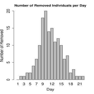
(a) Removals each day

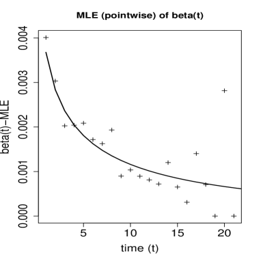
(b) True $\beta$ and ML estimates

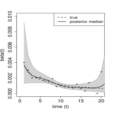
(c) Posterior $\beta$, infection times known

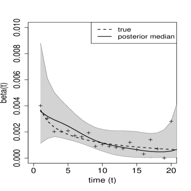
(d) Posterior $\beta$, infection times unknown

Figure 1: Results for simulated data in Scenario 1 using $\beta(t)=(0.01)\exp(-t^{1/3})$, $\gamma=0.5$, $N=500$, and GP prior covariance function values $\omega=10$, $l=6$. Plots (b) and (c) are obtained using the known true infection times, and plot (d) only uses the removal data. The shaded regions in (c) and (d) are 95% posterior credible intervals for $\beta$. The ML estimates are shown as crosses in (c) and (d) for comparison.

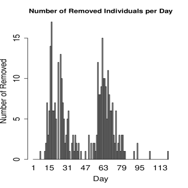
(a) Removals each day

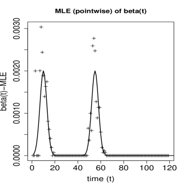
(b) True $\beta$ and ML estimates

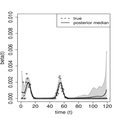
(c) Posterior $\beta$, infection times known

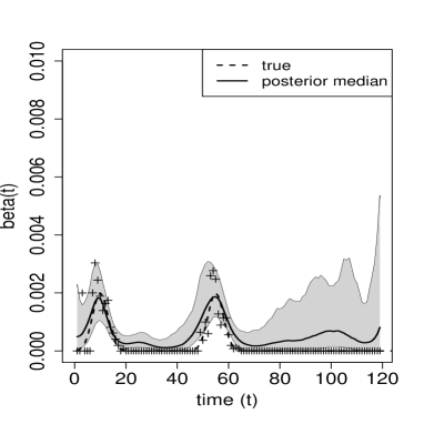
(d) Posterior $\beta$, infection times unknown

Figure 2: Results for simulated data in Scenario 2 using $\beta(t)=(0.002)\exp\left\{-(x-10)^{2}/18\right\}+(0.002)\exp\left\{-(x-55)^{2}/18\right\}$, $\gamma=0.1$, $N=500$, and GP prior covariance function values $\omega=8$, $l=5$. Plots (b) and (c) are obtained using the known true infection times, and plot (d) only uses the removal data. The shaded regions in (c) and (d) are 95% posterior credible intervals for $\beta$. The ML estimates are shown as crosses in (c) and (d) for comparison.

Smallpox data Our final example uses a classical data set collected during an outbreak of smallpox in the Nigerian town of Abakaliki in 1967 (Thompson and Foege,, 1968). These data have been considered by numerous authors, almost always to illustrate new statistical methodology, and are usually taken to consist of the symptom-appearance times of 30 individuals among a homogeneously-mixing susceptible population of 120 individuals. More extensive analyses of the full data set, which includes information on population structure, vaccination and other aspects, can be found in Eichner and Dietz (2003) and Stockdale et al. (2017). The results are shown in Figure 3, the key finding of which is that there is no evidence to suggest any material variation in the infection rate during the outbreak. For comparison with a continuous-time analysis, we include a figure from Xu, (2015) which uses the methods described in Section 3.2, so that the infection rate has a transformed GP prior. It is clear that this approach gives similar results to our discrete-time approach.

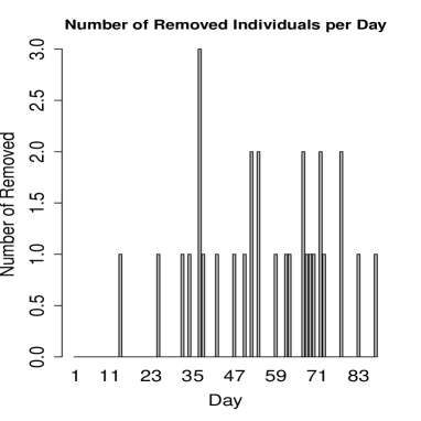
(a) Symptom-appearances each day

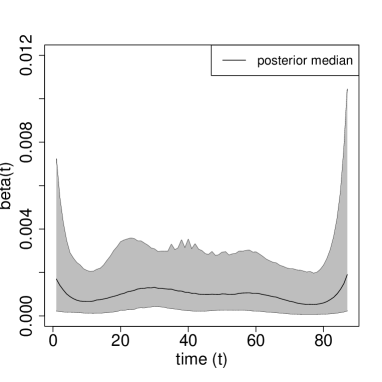
(b) Posterior median of $\beta$

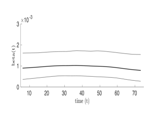
(c) Posterior mean of $\beta$, continuous-time analysis

Figure 3: Results for the Abakaliki smallpox data (a,b). Here $N=120$ and GP prior covariance function values are $\omega=5$, $l=14$. The shaded region in plot (b) shows the 95% credible interval for $\beta$. The figure in (c) is taken from a continuous-time analysis described in Xu, (2015) and shows the posterior mean and 95% credible interval for $\beta$.

5 Concluding comments

We have briefly described recently-developed methods for nonparametric Bayesian modelling and inference for epidemic models, specifically focussing on infection or incidence rate functions in SIR models. The methods themselves can easily be extended to other situations, including epidemic models in which there are several types of individuals with potentially different infectivity of susceptibility characteristics, or more complex models that include features such as latent periods or more realistic population structure. Some of these extensions are described in Xu, (2015) and Xu et al. (2016).

Other aspects of epidemic models could also be modelled nonparametrically. Boys and Giles, (2007) essentially do this by replacing the removal rate $\gamma Y(t)$ by a more flexible time-varying function modelled by a step-function. One motivation for doing this is to investigate the usual assumption that infectious periods are identically distributed. Another possibility is to model population structure nonparametrically. In general this appears to be a challenging problem, since it involves defining a suitable prior for population structure, which could itself be described by a network or random graph model. An approach involving the so-called Indian Buffet Process (IBP) is described in Ford (2014), in which the IBP is used as a model for a bipartite graph on which an epidemic spreads. However, the resulting inference problem generates many computational challenges.

References

- Adams et al. (2006) Adams, R. P., Murray, I., and MacKay, D. J. C. (2006). The Gaussian process density sampler. In Advances in Neural Information Processing Systems 21, Eds. Koller, D., Schuurmans, D., Bengio, Y. and Bottou, L., pp. 9–16.
- Adams et al. (2009) Adams, R. P., Murray, I., and MacKay, D. J. C. (2009). Tractable nonparametric Bayesian inference in Poisson processes with Gaussian process intensities. New York: ACM Press.
- Andersen et al. (1993) Andersen, P. K., Borgan, Ø, Gill, R. D. and Keiding, N. (1993). Statistical Models based on Counting Processes. New York: Springer.
- Andersson and Britton (2000) Andersson, H. and Britton, T. (2000). Stochastic Epidemic Models and their Statistical Analysis. Lecture Notes in Statistics, 151. New York: Springer.
- Bailey (1975) Bailey, N. T. J. (1975). The Mathematical Theory of Infectious Diseases and its Applications, 2nd ed. London: Griffin.
- Becker (1989) Becker, N. G. (1989). Analysis of Infectious Disease Data. London: Chapman and Hall.
- Becker and Yip (1989) Becker, N. G. and Yip, P. S. F. (1989). Analysis of variation in an infection rate. Australian Journal of Statistics 31, 42–52.
- Boys and Giles, (2007) Boys, R. J. and Giles, P. R. (2007). Bayesian inference for stochastic epidemic models with time-inhomogeneous removal rates. Journal of Mathematical Biology 55, 223–247.
- Chen et al. (2008) Chen, F., Huggins, R. M., Yip, P.S. and Lam, K. F. (2008). Nonparametric estimation of multiplicative counting process intensity functions with an application to the Beijing SARS epidemic. Communications in Statistics: Theory and Methods 37, 294–306.
- Eichner and Dietz (2003) Eichner, M. and Dietz, K. (2003). Transmission potential of smallpox: estimates based on detailed data from an outbreak. American Journal of Epidemiology 158, 110–117.
- Ford (2014) Ford, A. P. (2014) Epidemic models and MCMC inference. PhD Thesis, University of Warwick. http://webcat.warwick.ac.uk/record=b2752139~S1 .
- Knock and Kypraios (2016) Knock, E. S. and Kypraios, T. (2016). Bayesian non-parametric inference for infectious disease data. https://arxiv.org/abs/1411.2624.
- Lau and Yip (2008) Lau, E. H. Y. and Yip, P. S. F. (2008). Estimating the basic reproductive number in the general epidemic model with an unknown initial number of susceptible individuals. Scandinavian Journal of Statistics 35, 650–663.
- Lekone and Finkenstadt (2006) Lekone, P. E. and Finkenstädt, B. F. (2006). Statistical inference in a stochastic SEIR model with control intervention: Ebola as a case study. Biometrics 62, 1170–1177.
- McKinley et al. (2009) McKinley, T. J., Cook, A. R. and Deardon, R. (2009). Inference in epidemic models without likelihoods, The International Journal of Biostatistics 5(1).
- O’Neill and Roberts (1999) O’Neill, P. D. and Roberts, G. O. (1999). Bayesian inference for partially observed stochastic epidemics. Journal of the Royal Statistical Society Series A 162, 121–129.
- Pollicott et al. (2012) Pollicott, M. Wang, H. and Weiss, H. (2012). Extracting the time-dependent transmission rate from infection data via solution of an inverse ODE problem. Journal of Biological Dynamics 6, 509–523.
- Rasmussen and Williams (2006) Rasmussen, C. E. and Williams, C. K. I. (2006). Gaussian Processes for Machine Learning. Cambridge, Massachusetts: MIT Press.
- Smirnova and Tuncer (2014) Smirnova, A. and Tuncer, N. (2014). Estimating time-dependent transmission rate of avian influenza via stable numerical algorithm. Journal of Inverse and Ill-Posed Problems 22(1), 31–62.
- Stockdale et al. (2017) Stockdale, J. E., Kypraios, T. and O’Neill, P. D. (2017). Modelling and Bayesian analysis of the Abakaliki smallpox data. Epidemics, in press.
- Thompson and Foege, (1968) Thompson, D. and Foege, W. (1968). Faith Tabernacle smallpox epidemic. Abakaliki, Nigeria. World Health Organization.
- Xu, (2015) Xu, X. (2015). Bayesian Nonparametric Inference for Stochastic Epidemic Models. Ph.D. thesis, University of Nottingham. http://eprints.nottingham.ac.uk/29170/
- Xu et al. (2016) Xu, X., Kypraios, T. and O’Neill, P. D. (2016) Bayesian non-parametric inference for stochastic epidemic models using Gaussian processes. Biostatistics 17, 619–633.