Extinction in lower Hessenberg branching processes with countably many types
P. Braunsteins and S. Hautphenne
(March 10, 2024)
Abstract
We consider a class of branching processes with countably many types which we refer to as Lower Hessenberg branching processes. These are multitype Galton-Watson processes with typeset , in which individuals of type may give birth to offspring of type only. For this class of processes, we study the set of fixed points of the progeny generating function. In particular, we highlight the existence of a continuum of fixed points whose minimum is the global extinction probability vector and whose maximum is the partial extinction probability vector .
In the case where , we derive a global extinction criterion which holds under second moment conditions, and when we develop necessary and sufficient conditions for .
Keywords: infinite-type branching process; extinction probability; extinction criterion; fixed point; varying environment.
1 Introduction
Multitype Galton-Watson branching processes (MGWBPs) describe the evolution of a population of independent individuals who live for a single generation and, at death, randomly give birth to offspring that may be of various types.
Classical reference books on MGWBPs include Harris [21], Mode [29], Athreya and Ney [2], and Jagers [24].
MGWBPs have been used to model populations in several fields, including in molecular biology, ecology, epidemiology, and evolutionary theory, as well as in particle physics, chemistry, and computer science.
Recent books with a special emphasis on applications are Axelrod and Kimmel [3], and Haccou, Jagers and Vatutin [20].
Branching processes with an infinite number of types have been used to model the dynamics of escape mutants [35] and the spread of parasites through a host population [4, 5]; see also [3, Chapter 7] for other biological applications of infinite-type branching processes.
One of the main quantities of interest in a MGWBP is the probability that the population eventually becomes empty or extinct.
Let the vector record the number of type- individuals alive in generation of a population whose members take types that belong to the countable set .
We let
(1.1)
be the probability of global extinction given that the population begins with a single individual of type , and we refer to as the global extinction probability vector.
When the set contains only finitely many types, many of the fundamental questions concerning have been resolved. In particular, it is well known that (i) is the minimal non-negative solution of the fixed point equation ,
where , defined in (2.2), records the probability generating function associated with the reproduction law of each type, and that (ii) if the process is irreducible, then the set of fixed point solutions
(1.2)
contains at most two elements, and . In addition, there is a well-established extinction criterion, namely if and only if the Perron-Frobenius eigenvalue of the mean progeny matrix (defined in (2.3)) is less than or equal to one.
If we allow to contain countably infinitely many types then this complicates matters considerably.
Indeed, even the definition of extinction is no longer unambiguous.
We let
(1.3)
be the probability of partial extinction given that the population begins with a single individual of type , and we refer to as the partial extinction probability vector.
While global extinction implies partial extinction, there may be a positive chance that every type eventually disappears from the population while the total population size grows without bound; it is then possible that (see [22, Section 5.1] for an example).
At least partly due to these challenges, the set is yet to be fully characterised in the infinite-type setting.
There is, however, a number of papers that make progress toward this goal:
Moyal [30] gives general conditions for to contain at most a single solution such that ; Spataru [36] gives a stronger results by stating that contains at most two elements, and ; however, Bertacchi and Zucca
[8, 9] prove the inaccuracy of the latter by providing an irreducible example where contains uncountably many elements such that .
Both and are elements of the set . It is well known that is the minimal element, but as yet, there has been no attempt to identify the precise location of .
We observe that due to the existence of irreducible MGWBPs with , the partial extinction probability vector may be neither the minimal element of , which is , nor the maximal element of , which is .
Extending the extinction criterion established in the finite-type case to the infinite-type setting has also proven difficult.
To resolve the problem in the infinite-type setting we should give both a partial and a global extinction criterion.
A number of authors have progressed in this direction
[8, 12, 21, 22, 30, 36, 37].
In the infinite-type case, the analogue of the Perron-Frobenius eigenvalue is the convergence norm of defined in (2.4), which gives a partial extinction criterion: if and only if , see [37, Theorem 4.1].
However, when partial extinction is almost sure we are still lacking general necessary and sufficient conditions for . It turns out that
there can be no global extinction criterion based solely upon ,
as highlighted through [37, Example 4.4], but as pointed out by the author, other moment conditions have not been clearly identified.
In addition, when , following the terminology in [8], the process can exhibit strong local survival , or non-strong local survival . It is again challenging to derive a general criterion separating the two cases.
The main contribution of this paper is to use a unified probabilistic approach to characterise the set and to derive a global extinction criterion applicable when
for a class of branching processes with countably infinitely many types called lower Hessenberg branching processes (LHBPs). In these processes, which have the typeset , the primary constraint is that type- individuals can produce offspring of type no larger than ; as a consequence their (infinite) mean progeny matrices have a lower Hessenberg form.
The probabilistic approach we employ relies on a single pathwise argument: we reduce the study of the LHBP to that of a much simpler Galton-Watson process in a varying environment (GWPVE), embedded in the LHBP.
GWPVEs are single-type Galton-Watson processes whose offspring distributions vary deterministically with the generation.
In our context, the embedded GWPVE is explosive, in the sense that individuals may have an infinite number of offspring. In particular, we show the equivalence between global extinction of the LHBP and extinction of the embedded GWPVE, and between partial extinction of the LHBP and the event that all generations of the embedded GWPVE are finite.
Based on this relationship, we obtain several results for LHBPs:
(i)
We prove that there is a continuum of fixed points solutions , whose componentwise minimum and maximum are the global and partial extinction probability vectors and , respectively (Theorem 1).
(ii)
We establish a connection between the growth rates of the embedded GWPVE and the convergence rate of to as for any ; this yields a physical interpretation for the fixed points lying in between and (Theorem 4).
(iii)
In the non-trivial case where , we provide a necessary and sufficient condition for global extinction which holds under some second moment conditions (Theorem 5). This is the first extinction criterion for irreducible processes that also applies to cases exhibiting non exponential growth. We illustrate the broad applicability of the criterion through some examples.
(iv)
Finally, under additional assumptions, we build on the global extinction criterion to derive necessary and sufficient conditions for strong local survival (Theorem 8).
While there is a vast literature on GWPVEs, the explosive case,
which has already been studied for standard Galton-Watson processes [32, 33], is yet to be considered in the context of varying environment.
In order to prove our main theorems, we both apply known results on GWPVEs and develop new ones.
On the way to studying properties of the embedded GWPVE, we also derive a new partial extinction criterion for LHBPs which is computationally more efficient than other existing criteria.
The paper is organised as follows. In Section 2 we define LHBPs and introduce the tools we use to study them. In Section 3 we construct the embedded GWPVE and derive relationships between it and its corresponding LHBP. In Section 4 we develop (i) and (ii). In Section 5 we deal with (iii). In Section 6 we illustrate the results of Section 5 through two examples. In Section 7 we address (iv). Finally, in Section 8 we discuss possible extensions of our results.
In this paper, we let and denote the column vectors of ’s and ’s, respectively, and we let represent the vector with all entries equal to zero, except entry which is equal to 1, the size of these vectors being defined by the context. For any vectors and , we write if for all , and if with for at least one entry .
2 Preliminaries
Consider a MGWBP with the type set . We assume that the process initially contains a single individual whose type is denoted by . The process then evolves according to the following rules:
(i)
each individual lives for a single generation, and
(ii)
at death individuals of type give birth to offspring, that is, individuals of type , individuals of type , …, and individuals of type , where the vector is chosen independently of that of all other individuals according to a probability distribution, , specific to the parental type .
We refer to this as a lower Hessenberg branching process (LHBP).
We construct the LHBP on the Ulam-Harris space [21, Ch. VI], labelled , as follows. Let where describes the virtual -th generation. That is, , where specifies the type of the root, and for , , where denotes the -th child of type born to and denotes the individual’s unique identification number. Each virtual individual is assigned a random offspring vector that takes values in when is of type and has distribution
, independently of all other individuals. The random set of individuals who appear in the population, , is then defined recursively from the values of as follows
(2.1)
The population in generation is described by the vector with entries
We will often refer to branching processes by their sequence of population vectors .
We define the progeny generating vector , where
(2.2)
and the mean progeny matrix , where
(2.3)
is the expected number of type- children born to a parent of type .
By assumption, is an infinite lower Hessenberg matrix.
To avoid trivialities we assume that for all .
To , we associate a weighted directed graph, referred to as the mean progeny representation graph.
This graph has vertex set and contains an edge from to of weight if and only if .
The branching process is said to be irreducible if there is a path between any two vertices in the mean progeny representation graph on .
We define the convergence norm of ,
(2.4)
which, when the process is irreducible, is independent of and .
The global and partial extinction probability vectors and , defined in (1.1) and (1.3), are both solutions to the fixed point equation , and are thus elements of the set defined in (1.2).
This can be seen by conditioning on the children of the initial individual and then observing that the process becomes partially (globally) extinct if and only if the daughter processes of these children become partially (globally) extinct.
Moreover, following the standard arguments, we can prove that is the componentwise minimal element of (see [30, Theorem 3.1]).
By the lower Hessenberg assumption, can be written as for all . Thus, by the monotonicity of , each entry of any is uniquely determined by .
It is then natural to consider the one-dimensional projection sets of ,
Figure 2.1: The processes , and for a specific .
We define two sequences of finite-type branching processes on .
The first, , is such that the random offspring vector of any virtual individual is given by
for any , where is the type of virtual individual .
For any , outcomes of are thus constructed by taking the corresponding outcome of and removing the descendants of all individuals of type . These types are said to be sterile.
The second, , is such that the random offspring vector of any virtual individual is given by
for any .
For any , outcomes of are thus constructed by taking the corresponding outcome of and replacing the descendants of all individuals of type with an infinite string of type- descendants. These types are said to be immortal.
An illustration of , and for a specific is given in Figure 2.1.
By construction, for all , (i) for each fixed value of , if then the sterile and immortal individuals are necessarily of type , (ii)
(2.5)
and (iii)
(2.6)
We denote the progeny generating vector of by , which has entries
(2.7)
By Equation (2.5), the global extinction probability vectors of and , denoted by and , are given by
where is the -fold composition of .
As demonstrated in [22, Lemma 3.1], the sequence increases componentwise to . In addition, if is irreducible and non-singular (that is, there exists such that ), then the sequence decreases componentwise to (see Theorem 9 in Appendix A). Note that [22, Lemma 3.2] is an inaccurate version of the latter result.
Unless stated otherwise, we assume that is non-singular and irreducible.
3 An embedded GWPVE with explosions
Figure 3.1: An outcome of and for a specific . The highlighted type- individuals
represent the sterile individuals in the corresponding realisation of .
We construct the embedded GWPVE on from the paths of by selecting all individuals whose type is strictly larger than that of all their ancestors, and connecting each selected individual to their nearest (in generation) selected ancestor (see Figure 3.1).
More formally, we define a function that takes a line of descent and deletes each triple whose type is not strictly larger than all its ancestors.
For each the family tree of is then given by , where is defined in (2.1).
Variants of (which do not permit explosion) can be found in [12] and [19].
We take the convention that starts at the generation number corresponding to the initial type in . By construction, for any we then have
(3.1)
that is, the th generation of is made up every sterile (type-) individual produced over the lifetime of .
By the lower Hessenberg assumption, each sterile type- individual that appears in is a descendant of a sterile type- individual that appears in .
Thus, because the daughter processes of these type-() individuals in are i.i.d., satisfies the branching process equation
(3.2)
where is a sequence of i.i.d. random variables such that, conditional on .
This means is indeed a GWPVE;
it is however not a classical one because may have a positive chance of explosion, that is, individuals in may give birth to an infinite number of offspring with positive probability.
The next lemma states that explodes by generation if and only if survives globally, and becomes extinct by generation if and only if becomes globally extinct.
Lemma 1
For any ,
(3.3)
and
(3.4)
Proof:
To prove (3.3), first suppose that . Then there exists a generation such that for all . This means , which implies .
It then remains to prove
Because for any , we have
for some .
Thus, for any , we have
where .
By the Markov property, we then have
leading to (3.3). The same arguments lead to (3.4).
Since
and
the process has two absorbing states, and .
The next corollary formalises the equivalence between the following
events:
Corollary 1
The global extinction event , and the partial extinction event .
Proof:
The result follows from Lemma 1 and the arguments in the proofs of [22, Lemmas 3.1] and Theorem 9 respectively.
By Corollary 1 we can express any question about the extinction probability vectors and in terms of the process .
In the sequel we use the shorthand notation for and for .
Corollary 2
For any and ,
and for any ,
Proof:
The results are immediate consequences of Lemma 1 and Corollary 1.
To take advantage of Corollary 2 we require the progeny generating function of each generation of the embedded GWPVE.
For , we let
(3.5)
where .
Due to the possibility of explosion we may have .
By (3.2), the generating function of , conditional on for , is given by
The next two lemmas provide respectively an explicit and an implicit relation between the sequence of progeny generating functions and the progeny generating vector . The first requires the following technical assumption:
Assumption 1
For all ,
(3.6)
Lemma 2
If Assumption 1 holds,
then for all , the progeny generating function of at generation is given by
We now characterise the set defined in (1.2). The main results in this section rely on the relation between and the set
which corresponds to the set of fixed points of the embedded GWPVE. Because each is a monotone increasing function, like , the set is one-dimensional.
In this section we assume that Assumption 1 holds.
For any vector , we write for the restriction of to its first entries.
The next lemma establishes a relationship between and .
Lemma 4
Proof:
Suppose and .
For any , satisfies .
Because is irreducible and we have for all (see [36, Theorem 2]).
Thus, using Lemma 2,
for all , leading to .
Now suppose . Then, by Lemma 3, for all ,
therefore .
We now characterise the one-dimensional projection sets and identify which elements of correspond to the global and partial extinction probability vectors.
Theorem 1
If then ; otherwise
In particular,
Proof:
We show that
(4.1)
and for any ,
,
where
These results follow from the fact that and are monotone increasing functions, and therefore so are and for . Let , then for all ,
Taking the limit as we obtain for all , which shows (4.1).
Now suppose .
For any , define ; then
Similarly, for any , define ; then
This shows that for any and for any , it is possible to construct a vector belonging to .
Theorem 1 implies that contains one, two, or uncountably many elements. More specifically, it shows that is the minimal element of
which is the beginning of a continuum of elements whose supremum is , as illustrated in Figure 4.1.
Figure 4.1: A visual representation of possible sets in the irreducible case.
Remark 1
In the reducible case there may be an additional countable number of fixed points such that . We refer to [11, Section 4.4] for the details.
With the goal of giving a probabilistic interpretation to the intermediate fixed points such that ,
we now derive properties of the infinite-dimensional set .
We begin by deriving a sufficient condition for
(4.2)
that is, for to contain at most a single element (corresponding to ) whose entries do not converge to .
In a more general setting, sufficient conditions for (4.2) can be found in Moyal [30, Lemmas 3.3 and 3.4], the most notable being ‘’. The same author also conjectures a more general condition:
In the case of LHBPs we now provide a stronger result.
Proof:
Following Lindvall [26], we have if and only if
(4.4)
Suppose (4.3) holds without (4.4), that is, assume (4.3) and
(4.5)
In this case, there can be only finitely many such that .
Thus,
(4.5) holds if and only if there exists such that
(4.6)
In addition, because for all , in every generation of the embedded process (including any for which ) individuals have a positive chance of giving birth to at least one offspring. In combination with (4.6) this implies that there exists such that for any ,
Recall that each individual in corresponds to an individual in . If the corresponding individual in has no offspring then neither does the individual in , whereas if the corresponding individual in has two or more offspring then the individual in must have at least two offspring with probability greater than or equal to . Thus, for all ,
which implies
contradicting (4.5). Therefore, if (4.3) holds, we must have (4.4).
Proof of Theorem 2:
By Lemma 4, we may assume . Thus, for all
,
(4.7)
Suppose . In this case there exists an infinite sequence such that for all and some .
For each and ,
By Lemma 5, for any , we have as . Letting be arbitrarily large, we obtain
Because as , from (4.7) we then obtain . The only element such that is therefore .
Now that we have general sufficient conditions for , we investigate properties of this convergence.
The next two theorems use the following lemma.
Lemma 6
If and are sequences of non-negative real numbers such that for all , and , then
(4.8)
(4.9)
Proof:
For any we have
The result then follows from for any .
The next result shows that if the entries of converge to 1, then they converge slower than those of any other , whereas the entries of converge to faster than those of any other .
The next theorem demonstrates that the rate at which decays is closely linked to the asymptotic growth of . In this context, we define a growth rate to be a sequence of real numbers such that
where is a non-negative, potentially defective, random variable with
We let
Growth rates of non-defective GWPVEs () have been studied by a number of authors. Although it is natural to assume that
is a growth rate, it may not always be the case. Sufficient conditions for to be a growth rate are given in [23], and conditions for it to be the only distinct growth rate are discussed in [15, 16, 25]. Examples of GWPVEs with multiple growth rates can be found in [17, 27].
Theorem 4
Suppose (4.3) holds. If and there exists some growth rate such that , then
where is such that .
Proof:
By the arguments in the proof of Lemma 4, any is such that for all , and . Therefore, for all ,
(4.12)
which can be rewritten as
(4.13)
By assumption we have
(4.14)
If , then taking in (4.13) gives
which contradicts (4.14). A Similar argument applies to the limit superior, leading to
where (4.16) follows from the dominated convergence theorem, and (4.17) requires (4.15).
If we repeat the same argument with replaced by , we finally obtain
By (4.3) and Theorem 2 we have and thus through (4.15) we obtain . Lemma 6 then gives , where . This means
.
We conclude this section with a summary of our findings on the set .
The set is made up of a continuum of elements whose minimum is and whose maximum is , with the additional fixed point .
Under Condition (4.3), for any , with the possible exception of , we have as .
The decay rates of and are unique, whereas the intermediate elements may share one or several decay rates, which have a one-to-one correspondence with the growth rates of .
Furthermore, these intermediate elements completely specify the generating functions and thereby the distributions of .
This gives a physical meaning to the intermediate elements: in short, they describe the evolution of when there is partial extinction without global extinction.
While this physical interpretation is in terms of the growth of , we expect that it is closely related to the growth of .
5 Extinction Criteria
While there exist several well-established partial extinction criteria, determining a global extinction criterion when remains an open question.
When , the embedded GWPVE is non-explosive, and we can directly apply known extinction criteria for GWPVEs.
These criteria are generally expressed in terms of the first and second factorial moments
The next lemma provides recursive expressions for these moments in terms of those of the offspring distributions of .
We let
where
The assumption implies for all , and therefore
which leads to the expression for and the recursive Equation (5.3).
Next, by differentiating (5.5) with respect to , we obtain
where, for ,
This implies
which gives,
leading to the expression for and the recursive Equation (5.4).
When is not assumed, the recursive expressions (5.2)–(5.4) can still be used to compute two sequences, which may not correspond to the first and second factorial moments of the progeny distributions of , but which we shall even so denote by and .
For these sequences to correspond to well defined moments, their elements must be non-negative and finite, that is, the denominator common to (5.3) and (5.4) must be strictly greater than for all . Thus, if we let
we require
(5.6)
By giving a physical interpretation to , we now show that, in the irreducible case, (5.6) holds if and only if . Note that, if there exists such that , then , as justified in the proof of the lemma.
Lemma 8
If is irreducible then if and only if for all
Proof:
For any we embed a process
in by taking all type- individuals that appear in and defining the direct descendants of these individuals as the closest (in generation) type- descendants in ; the process evolves as a single-type Galton-Watson process that becomes extinct if and only if type becomes extinct in .
Because for all , the extinction of type in is almost surely equivalent to the extinction of the whole process . Hence, for any ,
where is the mean number of offspring born to an individual in .
The value of is obtained by taking the weighted sum of all first return paths to in the mean progeny representation graph of .
By conditioning on the progeny of an individual of type in , the lower-Hessenberg structure then leads to
Thus, if for all then for all , and therefore by Theorem 9, .
Similarly, if there exists such that , then .
Now suppose there exists such that . Then by the irreducibility of there exists such that there is a first return path with strictly positive weight of the form in the mean progeny representation graph of . This implies
and hence
Combining Lemmas 7 and 8 with [25, Theorem 1], which to the authors’ knowledge is the most general extinction criterion currently available for GWPVEs, we obtain for an irreducible LHBP:
Proof:
The global extinction criterion (5.8) follows from in [25, Theorem 1]. Indeed, our assumptions imply Condition (A) of that theorem, as well as .
Remark 2
Theorem 5 demonstrates that by computing the sequence
required for (5.8) we are implementing a partial extinction criterion.
We note that it is more efficient to compute through Lemma 7 than to evaluate the convergence norm of as the limit of the sequence of spectral radii of the north-west truncations of the mean progeny matrix (see [34, Theorem 6.8]).
Remark 3
If then, through the Markov inequality, we obtain . Thus, in this case the conditions of Theorem 5 do not need to be verified.
When the conditions of Theorem 5 do not hold, one may still be able to apply [25, Theorem 1] directly. Condition (A) in that theorem holds under an assumption on the third factorial moments ([25, Condition (C)]), which can also be shown to satisfy recursive equations.
Alternatively, it may be possible to apply
the next theorem, which corresponds to [1, Theorem 1] (see for example the proof of Proposition 1).
Theorem 6
If and for all , then for any ,
Roughly speaking, Theorem 5 states that the boundary between almost sure global extinction and potential global survival is the expected linear growth of , that is, , for some constant . It is however not immediately clear how to interpret this criteria in terms of the expected growth of the original LHBP .
The next theorem develops a link between the expected growth of and the exponential growth rate of the mean total population size in ,
(5.9)
which, when is irreducible, is independent of .
We note that in an irreducible MGWBP with finitely many types , whereas when there are infinitely many types it is possible that .
Theorem 7
Assume . If , then
(5.10)
and if , then
(5.11)
Proof:
We have , where ,
which gives
(5.12)
Now suppose . In order to prove (5.10) we need to show that
(5.13)
Indeed, if (5.13) holds, because we have
and thus by (5.12),
To show (5.13) assume there exists
and observe that for any the recursion
holds.
This implies that for all ,
and
which gives
By Equation (5.12) we then have for all ,
which contradicts the fact that and shows (5.13). When a similar argument can be used to obtain (5.11).
By Theorem 7, if both and exist (which is the case in our illustrative examples), then by the root test for convergence,
Thus, if then in Theorem 5
may be replaced by .
One contribution of Theorem 5, which is motivated by the examples in [7],
is to provide an extinction criterion applicable even when , as we demonstrate in Example 2.
6 Illustrative Examples
We now illustrate the results of the previous section through two examples.
Example 1 demonstrates that the mean progeny matrix is not sufficient to determine whether or .
This fact was highlighted in [37, Example 4.4], however, in that example, the process behaves asymptotically as a GWPVE because as . In addition, the proof relies on an explicit expression of the progeny generating vector.
Through Example 1 we provide a streamlined proof which applies to a significantly broader class of branching processes.
In Example 2 we apply Theorem 5 to a LHBP with . This example also motivates Section 7 on strong and non-strong local survival.
The proofs related to the examples are collected in Appendix B.
Example 1.
Consider a LHBP with mean progeny matrix
(6.1)
and progeny generating vector . We assume that and that there exists a constant such that
(6.2)
Apart from these assumptions, we impose no other condition on .
We now consider a modification of , which we denote by for some parameter , whose progeny generating vector, , is given by
(6.3)
This modification decreases the probability that a type- individual has any type- offspring by a factor of , but when the type- individual does have type- offspring, their number is increased by a factor of , which causes the mean progeny matrix to remain unchanged. Before providing results on the extinction of we require the following lemma on branching processes with the tridiagonal mean progeny matrix (6.1).
Lemma 9
Suppose has a mean progeny matrix given by (6.1), then
if and only if
Note that the partial extinction criterion (6.4) was given previously in [22] and is implied by [10, Theorem 1].
We are now in a position to characterise the global extinction probability of .
Proposition 1
Consider the branching processes defined in Example 1, and suppose and .
If then , whereas if , then
An important sub-case of Example 1 is , the set of unmodified branching processes.
Note that this is the only case where the second moments of the offspring distributions are uniformly bounded.
For this subclass of processes, when combined with Lemma 5, Proposition 1 yields
Example 2.
Let have a mean progeny matrix such that , and for ,
(6.6)
with all remaining entries being 0. The mean progeny representation graph corresponding to this process is illustrated in Figure 6.1. We assume that there exists such that for all and that .
For this example, it is not difficult to show that if and only if , which is the case for a range of values of , as we shall see.
Proposition 2
For the set of branching processes described in Example 2, if and only if .
Proposition 2 states that the process experiences almost sure global extinction if and only if
type- individuals can only have type- offspring, that is, if it coincides exactly with the embedded GWPVE.
Figure 6.1: The mean progeny representation graph corresponding to Example 2.
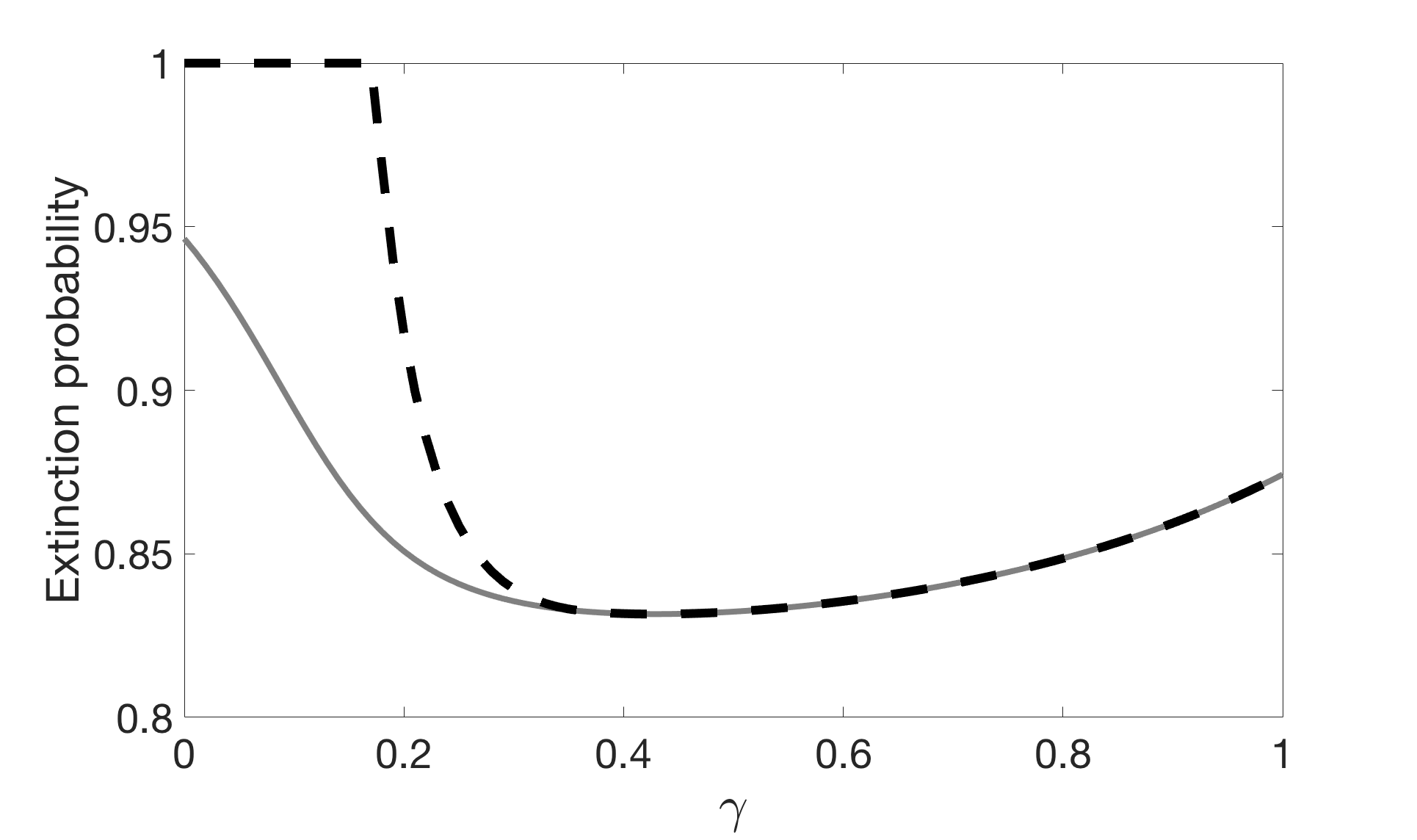
We choose
which satisfies (6.6), and in Figure 6.2 we plot and for . Although we proved that when , we observe that for this value of . This is because, when , Theorem 6 implies
so the convergence of to is slow. For GWPVEs with , little attention has been paid to this convergence rate in the literature, so for this example not much can be said when .
Using Lemmas 7 and 8 we numerically determine that if and only if where
(6.7)
Note that in this particular example a sufficient condition for is the existence of some such that (see the proof of Proposition 2). Thus, can be evaluated particularly efficiently.
Given , by visual inspection, the curves of partial and global extinction seem to merge from some value of , however the cut-off is not clear and further analysis is required to pinpoint the precise value.
We are also interested in understanding whether this value depends only on the mean progeny matrix or whether other offspring distributions lead to different values. We address these questions in the next section.
Figure 6.2: The extinction probabilities (solid) and (dashed) for .
7 Strong local survival
Each irreducible infinite-type branching process falls into one of the four categories , , or . The results in the previous section deal with the classification of LHBPs with . In the present section we build on these results to establish a method for determining whether LHBPs with experience strong local survival (), or non-strong local survival ().
Other attempts at distinguishing between these two cases can be found, for instance, in [8, 9] and [28].
For any , we partition into four components,
where is of dimension and the other three submatrices are infinite. We then construct a LHBP branching processes on , denoted as , with mean progeny matrix , and global and partial extinction probability vectors and , respectively. Sample paths of are constructed from those of by immediately killing all offspring of type , and relabelling the types so that type becomes . We now use to derive a criterion for strong local survival. In the next theorem we let denote the spectral radius.
Theorem 8
Assume that , that there exists such that
(7.1)
and that contains a finite number of strictly positive entries.
Then there is strong local survival in if and only if becomes globally extinct, that is,
(7.2)
Proof:
We use [9, Theorem 4.2] which we restate using our notation: let and be two branching processes on the countable type set with respective probability generating functions and , and global extinction probability vectors and . Let be a non-empty subset of types and denote by and the respective vectors of probability of local extinction in . If and differ on only, that is, if for all and for all , then
(7.3)
We apply this result with , , and being such that for all , that is, all types in are sterile. We need to show that (7.3) is equivalent to (7.2).
We first observe that since, by (7.1), in , types in are only able to survive through the presence of types in . Next, since types in are sterile in , if and only if for all . It is clear that by construction. It remains to show that . We couple the process and the process , . Let be the largest type in able to generate offspring in . Then since , with probability one there exists a generation such that for all . This implies that with probability one, for all , which shows .
When , we may apply Theorem 5 to determine whether .
We are now in a position to answer the questions posed at the end of the previous section.
The next result is proved in Appendix B.
Proposition 3
For the branching processes described in Example 2,
Proposition 3 demonstrates that the curves for partial and global extinction represented in Figure 6.2 merge at and that this value is independent of the particular offspring distributions. At the critical value there exists no satisfying (7.1), causing this case to remain untreated.
8 Conclusion
Besides thoroughly exploring the set of fixed-points for LHBPs, we have introduced a method of classifying LHBPs
into one of the categories , , or .Through Examples 1 and 2 we showed that our results can be used to rigorously determine which category the process falls in; however, in practical situations where rigorous proofs may not be possible, our results can still be applied computationally as a first step in classifying the process.
The inherent assumption in LHBPs is the constraint that individuals of type cannot give birth to offspring whose type is larger than for . The approach of embedding a GWPVE in the original LHBP can be extended to the case where takes any finite integer value. The resulting embedded GWPVE then becomes multitype with types. Results of Section 3 then naturally generalise, but those of Section 4 rely on the characterisation of the -dimensional projection sets of , which is more difficult in this case. The global extinction criterion discussed in Section 5 would now build upon extinction criteria for multitype GWPVE, which are less developed in the literature. These questions are the topic of a subsequent paper [13].
Appendix A: Partial extinction probability
The following result holds not only for LHBPs but in the more general setting of [22].
Theorem 9
If is irreducible and non-singular then componentwise as .
Proof:
Fix some initial type .
By construction, for every and , is increasing in , which implies is decreasing in . Similarly, if survives globally, then at least one type must survive in , which implies for all .
We may then assume .
Because is irreducible, [13, Corollary 1] implies that is equal to the probability that type eventually disappears from the population.
We define a function that takes lines of descent and deletes each triple whose type is not equal to , and we define the processes and , whose family trees are given by and , respectively. These are single-type Galton-Watson processes that become extinct if and only if type becomes extinct in and .
Thus, given the probability that becomes extinct is , and the probability that becomes extinct is greater than or equal to (if is reducible there may be a positive chance type dies out but survives globally).
Because is irreducible and non-singular, is non-singular, that is, there is positive chance that individuals in have a total number of offspring different from 1.
Thus, with probability 1, experiences extinction or unbounded growth [21, Chapter I, Theorem 6.2]. For any we then have
(.1)
Observe that, for any fixed and ,
and
(.2)
To understand (.2) observe that if , then there exists at least lines of descent such that the type is the th return to (where is not necessarily the same for each of these lines of descent).
By construction, the maximum type on each of these lines of descent is finite. Thus letting denote the maximum of the maximum type on arbitrarily selected such lines of descent, we see that .
We may now apply the monotone convergence theorem to obtain, for any ,
(.3)
The probability that becomes extinct is equal to that of , which is less than or equal the probability of extinction of the Galton-Watson branching process with progeny generating function
Therefore .
Observe that for any fixed the probability of extinction in a Galton-Watson process with progeny generating function converges monotonically to as (to see why note that for any there exists large enough to ensure ).
We are now in a position to show that for any there exists such that .
Given a process with partial extinction probability and some ,
we select by setting it large enough to ensure that a Galton-Watson branching process with progeny generating function has extinction probability less than .
By (.1), for this value of , we may select large enough to ensure . By (.3), for these values of and we may select large enough to ensure . By the triangle inequality and the preceding discussion, for these values of , , and , we have . The result then follows from the fact is decreasing in .
Appendix B: Proofs related to the examples
Proof of Lemma 9: Because (6.4) holds, Lemma 7 gives
(.4)
Because and
by induction the sequence is strictly positive and increasing.
Therefore, since ,
implies that converges to a finite limit ,
where satisfies the equation
which has real solutions
since (6.4) holds. When (6.4) holds we have
which, combined with (.4) and the fact that implies for all , hence .
Proof of Propostion 1:
Let . First, suppose . In this case we have
where follows from Lemma 9 and follows from the fact that the minimum number of type- offspring born to a type- parent is .
This then implies
and therefore by irreducibility.
Now suppose . Note that for all with the exception of .
Then, by Lemma 7,
for all and some , which implies
By assumption, and , thus . Using the fact that and the root test, we then obtain
If there exists such that , then by Lemma 8 we have . Assume from now on that , which implies that for all , and .
Since , using Equation (.5) we can inductively show that for all . We then have, for any ,
(.6)
The Raabe-Duhamel test for convergence ensures that ,
since for ,
To complete the proof, it remains to show that the condition in Theorem 5 holds.
By Lemma 7, for all ,
Since , the denominator is uniformly bounded away from 0; in addition, by assumption, for all , therefore
there exists some constant independent of such that
If (which we show below), then for large ,
Since , we have , which means that is a uniformly bounded sequence. Combining this with the fact that for all implies , and by Theorem 5.
Finally, we prove that . Observe that (.5) implies that if for some , then , and thus exists since for all .
Taking in (.5) we obtain that satisfies
which means is either or .
The function is convex, thus
for all ; in addition, by (.5), for all . These imply that if for some , then becomes negative for some , which is a contradiction. So the sequence lives in the open interval .
Let
be the solutions of the equation . By the convexity of for all , if there exists such that then is a decreasing sequence which converges to 1. Suppose . Then for some . We can then construct a LHBP, , stochastically smaller than by selecting a sufficiently large type and independently killing each type- child born to a type- parent with a probability carefully chosen to ensure . For this modified process we have , and repeating previous arguments, we obtain .
Proof of Proposition 3: Given Proposition 2 and Lemmas 7 and 8, it remains to show that for and for . Note that, in either case, since , In addition,
Since , we may choose small enough so that . By Lemma 9, this implies that for all , and
for all , where is computed using .
Assume first that . Then,
so we may choose small enough, corresponding to , so that for all and some . Hence there exists satisfying the conditions of Theorem 8 with .
Now suppose . If for any there exists such that
then by the recursion (.5) we have , for all
and the result is derived by repeating the steps that follow Equation (.6) in the proof of Proposition 2. Suppose instead that there exists such that for all . Then by Equation (.5) we have
which implies
(.7)
To show that this leads to a contradiction, we compare to a matrix with strictly smaller entries than : is such that , and for all , and ,
with all other entries 0. The value of , with computed using , then has a probabilistic interpretation: it is the probability that a simple random walk on the integers, with transition probabilities , whose initial value is 0, never hits . When it is well known that this value is non-zero. By the fact that we then have for all , which implies
contradicting (.7).
Acknowledgements
The authors are grateful to two anonymous referees for their constructive comments, which helped us to improve the manuscript. In particular, they thank the referee who pointed out the inaccuracy in [22, Lemma 3.2].
The authors would also like to acknowledge the support of the Australian Research Council (ARC) through the Centre of Excellence for the Mathematical and Statistical Frontiers (ACEMS). Sophie Hautphenne would further like to thank the ARC for support through Discovery Early Career Researcher Award DE150101044.
References
[1]Agresti, A.On the extinction times of varying and random environment branching processes.
Journal of Applied Probability, 12.1: 39–46, 1975.
[2]Athreya, K.B. and Ney, P.E.Branching Processes.
Springer, Berlin, 1972.
[3]Kimmel, M. and Axelrod, D.E.Branching Processes in Biology.
Springer, New York, 2002.
[4]Barbour, A. D.
Threshold phenomena in epidemic theory. In Probability, Statistics and Optimisation, 101-–116, Wiley, Chichester, 1994.
[5]Barbour, A. D., and Kafetzaki, M.A host-parasite model yielding heterogeneous parasite loads. Journal of mathematical biology, 31.2: 157–176, 1993.
[6]Bertacchi, D., and Zucca, F.Critical behaviors and critical values of branching random walks on multigraphs. Journal of Applied Probability, 45.02: 481–497, 2008.
[7]Bertacchi, D., and Zucca, F.Characterization of critical values of branching random walks on weighted graphs through infinite-type branching processes.Journal of statistical physics, 134.1: 53–65, 2009.
[8]Bertacchi, D. and Zucca, F.Strong local survival of branching random walks is not monotone.
Advances in Applied Probability, 46.2: 400–42, 2014.
[9]Bertacchi, D. and Zucca, F.A generating function approach to branching random walks.
Brazilian Journal of Probability and Statistics, 31.2: 229–253, 2017.
[10]Biggins, J. D., Lubachevsky, B. D., Shwartz, A., and Weiss, A.A branching random walk with a barrier.
The Annals of Applied Probability, 573–581, 1991.
[11]Braunsteins, P.Extinction in branching processes with
countably many types.
PhD dissertation, 2018.
[12]Braunsteins, P., Decrouez, G., and Hautphenne, S.A pathwise approach to the extinction of branching processes with countably many types.
Stochastic Processes and their Applications, to appear, 2018.
[13]Braunsteins, P., and Hautphenne, S.The probabilities of extinction in a branching
random walk on a strip, arXiv:1805.07634, 2018.
[14]Church, J. D.On infinite composition products of probability generating functions.
Probability Theory and Related Fields, 19.3: 243–256, 1971.
[15]D’Souza, J. C.The Rates of Growth of the Galton-Watson Process in Varying Environments.
Advances in Applied Probability, 26.03: 698-714, 1994.
[16]D’Souza, J. C., and Biggins, J. D.The supercritical Galton-Watson process in varying environments. Stochastic processes and their applications, 42.1: 39–47, 1992.
[17]Foster, J. H., and Goettge, R. T.The rates of growth of the Galton-Watson process in varying environment. Journal of Applied Probability, 13.01: 144-147, 1976.
[18]Gantert, N. and Müller, S.The critical branching Markov chain is transient.
Markov Processes and Related Fields, 12.4, 805–814, 2006.
[19]Gantert, N., Müller, S., Popov, S. and Vachkovskaia, M. Survival of branching random walks in random environment.
Journal of Theoretical Probability, 23.4, 1002–1014, 2010.
[20]Haccou, P., Jagers, P. and Vatutin, V. A.Branching processes: variation, growth, and extinction of populations. No. 5. Cambridge University Press, 2005.
[21]Harris, T. E.The theory of branching processes. Springer Berlin Heidelberg, 1963.
[22]Hautphenne, S., Latouche, G. and Nguyen, G.
Extinction probabilities of branching processes with countably infinitely many types.
Advances in Applied Probability, 45.4, 1068–1082, 2013.
[23]Jagers, P.Galton-Watson processes in varying environments. Journal of Applied Probability: 174-178, 1974.
[24]Jagers, P. Branching Processes with Biological Applications.
Wiley, London, 1975.
[25]Kersting, G.A unifying approach to branching processes in varying environments. arXiv:1703.01960, 2017.
[26]Lindvall, T.Almost sure convergence of branching processes in varying and random environments. The Annals of Probability, 344–346, 1974.
[27]MacPhee, I. M., and Schuh, H. J.A Galton-Watson branching process in varying environment with essentially constant offspring mean and two rates of growth. Australian & New Zealand Journal of Statistics, 25.2: 329–338, 1983.
[28]Menshikov, M. V. and Volkov, S. E.Branching Markov chains: qualitative characteristics.
Markov Process. Related Fields3.2: 225-241, 1997.
[29]Mode, C.J.Multitype Branching Processes.
Elsevier, New York, 1971.
[30]Moyal, J. E.Multiplicative population chains.
Proceedings of the Royal Society of London. Series A,
Mathematical and Physical Sciences,266, 518–526, 1962.
[31]Sagitov, S.Tail generating functions for the extendable branching processes.
Stochastic Processes and their Applications, 127.5, 2017.
[32]Sagitov, S. and Lindo, A.A special family of Galton-Watson processes with explosions.Branching Processes and Their Applications. Springer, 237–254, 2016.
[33]Sagitov, S. and Minuesa, C.Defective Galton-Watson processes.
arXiv:1612.03588v1, 2016.
[34]Seneta, E.Non-negative matrices and Markov chains.
Springer Science and Business Media, 2006.
[35]Serra, M.C. and Haccou, P.Dynamics of escape mutants.
Theoretical population biology, 72.1,167–178, 2007.
[36]Spataru, A.Properties of branching processes with denumerably many types.
Revue Roumaine de Mathématiques Pures et Appliquées (Romanian Journal of Pure and Applied Mathematics), 34, 747–759, 1989.
[37]Zucca, F.Survival, extinction and approximation of discrete-time branching random walks.
Journal of Statistical Physics 142.4: 726-753, 2011.