Climbing a shaky ladder:
Better adaptive risk estimation
Abstract
We revisit the leaderboard problem introduced by Blum and Hardt (2015) in an effort to reduce overfitting in machine learning benchmarks. We show that a randomized version of their Ladder algorithm achieves leaderboard error compared with the previous best rate of
Short of proving that our algorithm is optimal, we point out a major obstacle toward further progress. Specifically, any improvement to our upper bound would lead to asymptotic improvements in the general adaptive estimation setting as have remained elusive in recent years. This connection also directly leads to lower bounds for specific classes of algorithms. In particular, we exhibit a new attack on the leaderboard algorithm that both theoretically and empirically distinguishes between our algorithm and previous leaderboard algorithms.
1 Introduction
Machine learning benchmarks across industry and science are largely based on the simple mechanism of a holdout set. Participants repeatedly evaluate their models on the holdout set and use the feedback to improve their models. This feedback loop has become the de facto experimental paradigm in machine learning. What is concerning is that the analyst uses the holdout in a sequential and adaptive manner, thus creating dependencies between the model to be evaluated and the holdout data. The lack of independence between model and holdout data is what invalidates classical confidence bounds for the holdout setting. This insight was articulated in sequence of papers on what is now called adaptive data analysis [DFH+1, HU, DFH+2]. In a general formulation, adaptive data analysis can be thought of as an interaction between an algorithm that holds the sample, and an analyst that repeatedly asks queries about the data, such as “What is the loss of this model on the underlying population?”
In its general formulation, adaptive data analysis runs into strong computational lower bounds. Under computational hardness assumptions, no computationally efficient algorithm working with samples can preserve even mild statistical validity on more than queries [HU, SU]. This stands in sharp contrast to the non-adaptive setting where the error bounds deteriorate logarithmically with the number of queries
Circumventing these lower bounds, Blum and Hardt [BH] introduced a simpler setting that allowed for much better guarantees. The key idea is that oftentimes it’s sufficient to find the best model out of a sequence of adaptively chosen models, or to keep a ranking of some of the models. This is the relevant task in machine learning benchmarks, competitions, and hyperparameter tuning. Even adaptive early stopping can be posed as an instance of this problem. Within this framework, there’s a particularly simple and efficient algorithm called the Ladder algorithm. The algorithm maintains an internal threshold. Whenever a given model exceeds the previous quality threshold by a significant amount, the algorithm updates the threshold and provides the analyst with feedback about the quality of the model. If the model did not exceed the threshold, the analyst receives no feedback at all.
The Ladder algorithm maintains the risk of the best model (with respect to a bounded loss function) on a sequence of adaptively chosen models up to an additive error of This type of guarantee is called leaderboard error, since it does not require an accurate estimate for all models, but only the best performing one at any point in time. While this bound features a logarithmic dependence on the rate in terms of falls short of the non-adaptive bound
1.1 Our contributions
We narrow the gap between existing upper and lower bounds. Our first result is a randomized variant of the Ladder algorithm, called Shaky Ladder that achieves leaderboard error
Theorem 1.1 (Informal version of Theorem 2.7).
On samples and adaptively chosen models, the Shaky Ladder achieves with high probability leaderboard error
The algorithm is based on analyzing noise addition via differential privacy, in particular, the so-called sparse vector technique as described in [DR]. We combine this analysis with powerful adaptive generalization bounds for differential privacy, where it is important to use the recently improved bound of Bassily et al. [BNS+]. The earlier bound due to Dwork et al. [DFH+1] would not suffice to give any improvement over the Ladder algorithm that achieved leaderboard error
Our upper bound falls short of the information-theoretic lower bound of that holds even in the non-adaptive estimation setting. Intuition from online learning and the literature on bandit algorithms suggest that either the exponent or the exponent could be a natural answer. Surprisingly, our result shows that a natural algorithm achieves the unusual rate of Moreover, we show that going beyond this rate will likely require powerful new techniques.
In order to make this point, we develop a new connection between leaderboard and the general adaptive estimation setting. Specifically, we show that any accurate leaderboard algorithm for sufficiently many queries readily implies a general adaptive estimator (formally introduced in Section 3) for a smaller number of queries.
Theorem 1.2 (Informal version of Theorem 3.3).
Suppose there exists a leaderboard algorithm that is -accurate on samples and models. Then, there exists a general adaptive estimator that is -accurate on queries.
In the regime where , the best current upper bound is For this bound simplifies to and thus coincides with what would follow from our theorem. This is no coincidence since the bounds are proved using the same techniques. What is new, however, is that any further improvement in leaderboard accuracy over our result would directly improve on the best known bounds in the general adaptive estimation setting. In particular, a leaderboard upper bound of as is currently not ruled out, would lead to a general adaptive estimator for nearly queries and accuracy Going to the natural statistical rate of has remained elusive in the general adaptive estimation setting for any with . What our result shows is that this task is no easier in the leaderboard setting. It’s worth noting that there are lower bounds in special cases, e.g., [RZ, WLF].
We use Theorem 3.3 to prove a lower bound against a natural class of leaderboard algorithms that we call faithful. Intuitively, speaking when faithful algorithms return feedback, the feedback is close to the empirical risk of the submitted model with high probability. This class of algorithms includes both the Ladder algorithm and it’s heuristic counterpart the parameter-free Ladder. While those algorithms are deterministic, faithful algorithms may also be randomized.
Theorem 1.3 (Informal version of Corollary 3.12).
No faithful algorithm can achieve leaderboard error
In particular, this theorem separates our algorithm from earlier work. In Section 4, we illustrate this separation with a practical attack that causes a major bias in the Ladder algorithm, while being ineffective against our algorithm.
Beyond the related work already discussed, Neto et al. [NHB+] proposed a number of heuristic leaderboard algorithms based on the idea of replacing the holdout estimate by Bootstrap estimates. In practice, this results in noise addition that can be helpful. However, these algorithms do not come with theoretical bound on the leaderboard error better than the Ladder.
1.2 Preliminaries
Let be a data domain and be a finite set of class labels, e.g., and A loss function is a mapping and a model is a mapping A standard loss function is the -loss defined as if and otherwise. Throughout this paper we assume that is a loss function with bounded range. We assume that we are given a sample drawn i.i.d. from an unknown distribution over The risk of a model is defined as its expected loss on the unknown distribution The empirical risk is the standard way of estimating risk from a sample.
Adaptive risk estimation.
Given a sequence of models and a finite sample of size a fundamental estimation problem is to compute estimates of the risk of each model. Classically, this is done via the empirical risk. Applying Hoeffding’s bound to each empirical risk estimate, and taking a union bound over all functions, reveals that the largest deviation of any such estimate is bounded by This is the estimation error we expect to see in the standard non-adaptive setting.
In the adaptive estimation setting, we assume that the model may be chosen by an analyst as a function of previously observed estimates and previously chosen models. Formally, there exists a mapping such that for all the mapping returns a function from all previously observed information. We will assume for simplicity that the analyst is a deterministic algorithm. The tuple is nevertheless a random variable due to the random sample used to compute the estimates, as well possibly additional randomness introduced in the estimates. A natural notion of estimation error in the adaptive setting is the maximum error of any of the estimates, i.e., Unfortunately, lower bounds [HU, SU] show that no computationally efficient estimator can achieve maximum error on more than adaptively chosen functions (under a standard hardness assumption).
Leaderboard error.
Blum and Hardt [BH] introduced a weaker notion of estimation error called leaderboard error. Informally speaking, leaderboard error asks us to maintain a good estimate of the best (lowest risk) model seen so far, but does not require an accurate estimate for all models that we encounter.
Definition 1.4 (Leaderboard error).
Given an adaptively chosen sequence of models we define the leaderboard error of estimates as
| (1) |
2 The Shaky Ladder algorithm
We introduce an algorithm called Shaky Ladder that achieves small leaderboard accuracy. The algorithm is very simple. For each given function, it compares the empirical risk of the function to the previously smallest empirical risk plus some noise variables. If the estimate is below the previous best by some margin, it releases the estimate plus noise and updates the best estimate. Importantly, if the estimate is not smaller by a margin, the algorithm releases the previous best risk (rather than the new estimate). A formal description follows in Figure 1. For simplicity we assume we know an upper bound on the total number of rounds.
Input: Data sets with step size parameters Let Algorithm: – Assign initial estimate – Sample noise – For each round 1. Receive function 2. Sample noise variables independently. 3. If (a) (b) 4. Else assign 5. Output
Parameter settings.
We introduce a new parameter for the failure probability of our algorithm. For the purpose of our analysis we fix the parameters as follows:
| (2) |
With these settings all parameters are frozen with the one expection of The settings are optimized to prove the theorem, and do not necessarily reflect a good choice for practical settings. We will revisit this question in a later section.
From here on we let denote the number of update rounds of the algorithm:
| (3) |
We can quantify the privacy guarantee of the algorithm in terms of this parameter.
Lemma 2.1.
Algorithm 1 is -differentially private.
Proof.
For the purpose of its privacy analysis, the algorithm is equivalent to the algorithm “NumericSparse” in [DR] whose guarantees follow from the sparse vector technique. The only difference in our algorithm is that the threshold at each step varies. This difference is irrelevant for the privacy analysis, since only the parameter matters.
Since and are related multiplicatively through we can absorb all constant factors appearing in the analysis of “NumericSparse” in the -term. ∎
Our goal is to invoke a “transfer theorem” that translates the privacy guarantee of the algorithm into a generalization bound for the adaptive setting. The following theorem due to Bassily et al. [BNS+] intuitively shows that an -differentially private algorithm is unable to find a function that generalizes poorly.
Theorem 2.2 (Theorem 7.2 in [BNS+]).
Let and . Let be an -differentially private algorithm that, on input of a sample of size drawn i.i.d. from the population returns a function Then,
The original theorem is stated slightly differently. This version follows from the fact that the empirical risk with respect to a bounded loss function has “sensitivity” in the terminology of [BNS+].
Relevant to us is the following corollary.
Corollary 2.3.
Let be the functions encountered by the Shaky Ladder algorithm (Figure 1). Then, taking probability over both the sample and the randomness of the algorithm, we have
Proof.
Let and To apply Theorem 2.2 we need to observe that the composition of the Shaky Ladder algorithm with an arbitrary analyst (who does not otherwise have access to the sample ) satifies -differential privacy at every step of the algorithm. Hence, every function is generated by an -differentially private algorithm so that the theorem applies. The corollary now follows from a union bound over all functions. ∎
Lemma 2.4.
Let be all the Laplacian variables generated by our algorithm and consider the maximum absolute value Then,
Proof.
In the comparison step of the algorithm at step , note that
where Here we used Corollary 2.3, as well as our bound on the Laplacian random variables. Similarly, if we update at step , we have that
Hence, we can think of our algorithm as observing the population risk of each classifier up to the specified error bound. This implies, by induction, that the estimates achieve the specified leaderboard error. ∎
We have the following tail bound for the quantity that appeared in Lemma 2.4.
Lemma 2.5.
For every
Proof.
Note that is the maximum of at most centered Laplacian random variables with standard deviation For a single such random variable, we have
The claim now follows by applying this bound with and taking a union bound over all Laplacian variables which is the maximum of. ∎
We also need to bound the number of update steps This is easy to do assuming we have a bound on
Lemma 2.6.
Proof.
Assume that This implies that whenever satisfies
| (4) |
we must also have Since we also have Therefore, In particular, we can have at most rounds for which the event (4) occurs. ∎
Theorem 2.7.
There is a constant such that with suitably chosen parameter settings the Shaky Ladder algorithm (Figure 1) satisfies for any sequence of adaptively chosen classifiers
Proof.
Consider the event that simultaneously and Invoking our tail bounds from Lemma 2.5 and Lemma 2.4, we have that
Here we used the definition of and the fact that
Proceeding under the condition that occurs, we can plug in our parameter settings from Equation 2 to verify that
Rescaling to eliminate the constant in front of the error probability bound establishes the bound claimed in the theorem. ∎
3 Connection to general adaptive estimation
In the general adaptive estimation setting, the adaptive analyst choose a sequence of bounded functions usually called queries. The algorithm must return estimates in an online fashion such that each estimate is close to the population expectation We will refer to algorithms in this setting as general adaptive estimators to distinguish them from leaderboard algorithms that we studied earlier. The following definition of accuracy is common in the literature.
Definition 3.1.
We say that a general adaptive estimator is -accurate on samples and queries if for every distribution over given samples from the distribution and adaptively chosen queries the algorithm returns estimates such that
To bear out the connection with the leaderboard setting, we introduce an analogous definition for leaderboard error.
Definition 3.2.
We say that a leaderboard algorithm is -accurate on samples and classifiers if for every distribution over and every bounded loss function, given samples and adaptively chosen sequence of classifiers the algorithm returns estimates such that
Given these definition, we can show a reduction from designing general adaptive estimators to designing leaderboard algorithms in the regime where the number of queries is small.
Theorem 3.3.
Suppose there exists a leaderboard algorithm that is -accurate on samples and classifiers. Then, there exists a general adaptive estimator that is -accurate on queries. Moreover if is computationally efficient, then so is
Proof.
Assume the existence of and construct as follows. Let be the distribution over for which needs to be accurate. Take the range and let the loss function be With this loss function, we can think of a query as a classifier that satisfies
At each step the algorithm receives a query from an adaptive analyst and has to use the algorithm to answer the query. The algorithm is described in Figure 2. Note that all functions constructed in this procedure range in
Our first claim shows that if has small leaderboard error, then the answers extracted from the above procedure are accurate.
Claim 3.4.
If has leaderboard error then
Proof.
First note that by construction
By the definition of leaderboard error and our assumption, if the algorithm must output a value that is lower than and moreover satisfies By definition, and therefore,
Hence,
∎
Our second claim ensures that we don’t lower the threshold too quickly, thus allowing to answer sufficiently many queries.
Claim 3.5.
If has leaderboard error then the procedure we run for each function lowers the threshold by at most
Proof.
Observe that In other words, the difference in risk of any two consecutive classifiers is bounded by Hence, Therefore, the threshold can decrease by at most ∎
Assuming has leaderboard error the previous claim implies that the algorithm can use the algorithm for up to queries before the threshold reaches The total number of classifiers that gives to is bounded by ∎
It is natural to ask if the converse of the theorem is also true. Ideally, we would like to have a result showing that a general adaptive estimator for few queries implies a leaderboard algorithm for many queries. However, at this level of generality it is not clear why there should be such an argument to amplify the number of queries. Of course, by definition, we can say that a general adaptive estimator for queries implies a leaderboard algorithm for queries with the same accuracy.
Input: Data sets with blackbox access to algorithm Algorithm : Given the query the algorithm runs the following sequence of queries against – Set the threshold to be the last value that returned. If has not previously been invoked, set – For to – Construct the function – Give the function to and observe its answer – If put and stop. Else, continue.
3.1 Lower bounds for faithful algorithms
In this section, we prove a lower bound on a natural class of leaderboard algorithms that we call faithful. It includes both of the algorithms proposed by Blum and Hardt, the Ladder and the parameter-free Ladder algorithm. Both of these algorithms are deterministic, but the class of faithful algorithms also includes many natural randomization schemes.
Definition 3.6.
A leaderboard algorithm is faithful if given a sample of size for every adaptively chosen sequence of models its estimates satisfy with probability for all such that we also have
In words, given that the algorithm updated its estimate, i.e., the new estimate is likely close to the empirical risk of the -th model. The constants in the definition are somewhat arbitrary. Other choices are possible. What matters is that the algorithm returns something close to the empirical risk with reasonably high probability whenever it gives feedback at all.
To prove a lower bound against faithful algorithms, we will invoke our connection with the general estimation setting.
Definition 3.7.
A general adaptive estimator is faithful if given a sample of size for every sequence of adaptively chosen function its estimates satisfy with probability
The reduction we saw earlier preserves faithfulness.
Lemma 3.8.
If is a faithful leaderboard algorithm, then the algorithm resulting from the reduction in Figure 2 is a faithful general adaptive estimator.
We can therefore obtain a lower bound on faithful leaderboard algorithms by proving one against faithful general adaptive estimators.
Theorem 3.9.
No faithful general adaptive estimator is -accurate on samples and queries.
Proof.
Set up the distribution over with the label set such that the label is uniformly random conditional on any instance Fix a general adaptive estimator that gets a sample of size drawn from We need to show that the estimator cannot be -accurate. To show this claim we will analyze the following procedure (majority attack):
-
–
Pick random functions .
-
–
Let be the empirical risk of with respect to the -loss. Further, let be the answer from the general adaptive estimator on the query
-
–
Consider the index set
-
–
Let be the pointwise majority function of all functions in . That is is the majority value among with
-
–
Ask to estimate the -loss of i.e., submit the query
Note that and hence it remains to analyze the difference between the risk and empirical risk of
Claim 3.10.
Proof.
This is true for any function given the way we chose the distribution over ∎
We claim that the empirical risk is bounded away from by with constant probability. A similar claim appeared in [BH] without proof.
Claim 3.11.
Assume Then, with probability
Proof.
Following Definition 3.7, condition on the event that for all we have By the definition, this even occurs with probability Under this condition all satisfy Furthermore, we claim that with probability This follows because In particular both events occur with probability at least Let
be the advantage over random of in correctly labeling an element of By definition of we must have that for all We will argue that this advantage over random is amplified by the majority vote.
Let be the indicator of the event that for random For ease of notation rearrange indices such that where as argued earlier. We know that is Bernoulli with parameter where by construction Let be the indicator of the event that Let and observe that since Therefore,
| (Claim A.1, using ) | ||||
The claim now follows, since ∎
Taking Claim 3.10 and Claim 3.11 together, we have that with probability In particular, when this shows that the estimator is not -accurate. For the same claim follows from a standard variance calculation. ∎
The previous theorem implies that faithful leaderboard algorithms cannot have leaderboard error better than
Corollary 3.12.
No faithful leaderboard algorithm is -accurate on samples and queries for any and constant
Proof.
Combine our lower bound from Theorem 3.9 with the reduction in Theorem 3.3. By Lemma 3.8, faithfulness is preserved and hence we get the stated lower bound. ∎
4 Experiments with a shifted majority attack
The attack implicit in Corollary 3.12 corresponds to what we will call the shifted majority attack. To understand the idea, we briefly review the Boosting attack from [BH]. In this procedure, the analyst first asks random queries (thought of as vectors in , one binary label for each point in the holdout set), and then selects the ones that have error (-loss) less than Note that the expected loss is Among these selected queries, the analyst computes a coordinate-wise majority vote, resulting in a final output vector Blum and Hardt observed that this output vector has expected error with respect to the true holdout labels Despite the fact that the vector setup is a slight simplification of the actual formal framework we have, this idea carries over to our setting by replacing random vectors with random functions. We will refer to this procedure as majority attack.
The majority attack has the property that when run against the Ladder algorithm, the analyst quickly stops receiving new feedback. Newly chosen random functions are increasingly unlikely to improve upon the error of previous functions. Our procedure in Figure 2, however, shows how to offset the queries in such a way that the analyst continues to receive as much feedback as possible from the algorithm. In theory, this requires knowledge about the underlying distribution (which is fine for the purpose of proving the theorem). In reality, we can imagine that there may be a subset of the domain on which the classification problem is easy so that the analyst knows a fraction of the labels with near certainty. The analyst can then use this “easy set” to offset the functions as required by the attack. This leads to what we call the shifted majority attack.
Setup.
Rather than running the shifted majority attack, we will run the majority attack for a varying number of queries The reason for this setup is that there is no canonical parameter choice for the implementation of the Ladder algorithm, or the Shaky Ladder. In particular, the number of queries that can be answered using the shifting idea is closely related to the inverse of the step size parameter. It is therefore more transparent to leave the number of queries as a parameter that can be varied. Section B contains a reference implementation of the majority attack that we experiment with.
The primary purpose of our experiments is to understand in simulation the effect of adding noise to the feedback of the leaderboard algorithm.
Observations.
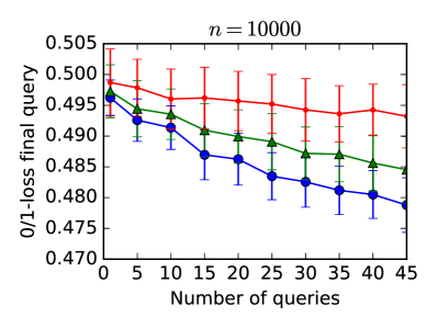
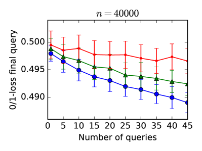
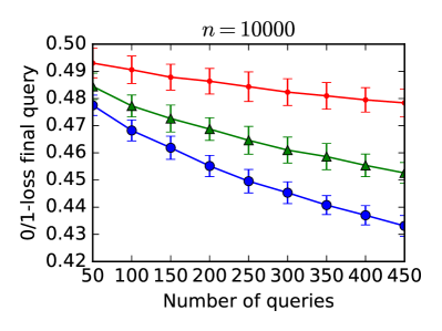
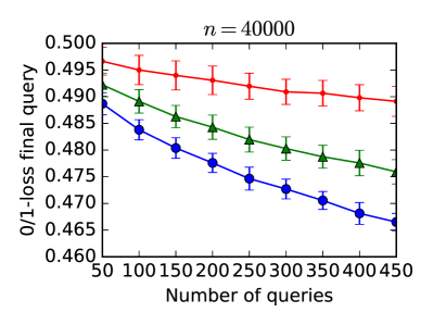
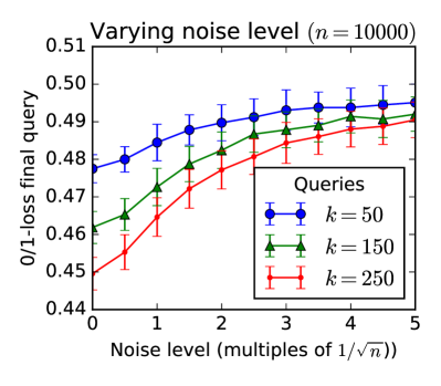
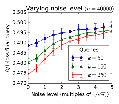
Figure 3 shows that even a small amount of Gaussian noise (e.g., standard deviation ) mostly neutralizes the majority attack that is otherwise very effective against the standard Ladder algorithm. We note in passing that the parameter-free Ladder algorithm [BH] only reveals more feedback than the Ladder algorithm. As such it fares even more poorly than the Ladder algorithm under the shifted majority attack.
Figure 4 consolidates the observation by showing the effect of varying noise levels. There appears to be a sweet spot at standard deviations, where much of the harm of the shifted majority attack is neutralized, while the amount of noise added is still small as a function of In particular, in simulation it appears that less noise is necessary than our theorem suggests.
5 Conclusion and open problems
We saw a new algorithm with leaderboard error This upper bound lies strictly between the two more natural bounds of and If experience from online and Bandit learning is any guide, the new upper bound might suggest that there is hope of attaining the tight error rate. This possibility is further supported by the fact that the majority attack we saw in Section 4 is quite sensitive to noise on the order of This leads us to conjecture that might in fact be the right answer. However, in light of our connection between the general adaptive estimation setting and leaderboard error, such a conjecture can now be refuted by stronger lower bounds for the general adaptive estimation setting. It is unclear if more sophisticated lower bounding techniques based on Fingerprinting codes as used in [HU, SU] could be used to obtain stronger lower bounds in the small number of query regime ().
Acknowledgments
Many thanks to Avrim Blum, Yair Carmon, Roy Frostig, and Tomer Koren for insightful observations and suggestions at various stages of this work.
References
- [BH] Avrim Blum and Moritz Hardt. The Ladder: A reliable leaderboard for machine learning competitions. In Proc. nd ICML, pages 1006–1014. JMLR.org, 2015.
- [BNS+] Raef Bassily, Kobbi Nissim, Adam D. Smith, Thomas Steinke, Uri Stemmer, and Jonathan Ullman. Algorithmic stability for adaptive data analysis. In Proc. th STOC, pages 1046–1059. ACM, 2016.
- [DFH+1] Cynthia Dwork, Vitaly Feldman, Moritz Hardt, Toniann Pitassi, Omer Reingold, and Aaron Roth. Preserving validity in adaptive data analysis. In Proc. th STOC, pages 117–126. ACM, 2015.
- [DFH+2] Cynthia Dwork, Vitaly Feldman, Moritz Hardt, Toniann Pitassi, Omer Reingold, and Aaron Roth. The reusable holdout: Preserving validity in adaptive data analysis. Science, 349(6248):636–638, 2015.
- [DR] Cynthia Dwork and Aaron Roth. The algorithmic foundations of differential privacy. Foundations and Trends in Theoretical Computer Science, 9(3-4):211–407, 2014.
- [HU] Moritz Hardt and Jonathan Ullman. Preventing false discovery in interactive data analysis is hard. In Proc. th FOCS, pages 454–463. IEEE, 2014.
- [NHB+] Elias Chaibub Neto, Bruce R Hoff, Chris Bare, Brian M Bot, Thomas Yu, Lara Magravite, Andrew D Trister, Thea Norman, Pablo Meyer, Julio Saez-Rodrigues, James C Costello, Justin Guinney, and Gustavo Stolovitzky. Reducing overfitting in challenge-based competitions. CoRR, abs/1607.00091, 2016.
- [RZ] Daniel Russo and James Zou. How much does your data exploration overfit? controlling bias via information usage. CoRR, abs/1511.05219, 201.
- [SU] Thomas Steinke and Jonathan Ullman. Interactive fingerprinting codes and the hardness of preventing false discovery. CoRR, abs/1410.1228, 2014.
- [WLF] Yu-Xiang Wang, Jing Lei, and Stephen E. Fienberg. A minimax theory for adaptive data analysis. CoRR, abs/1602.04287, 2016.
Appendix A Anti-concentration inequality for the Binomial distribution
Claim A.1.
Let Then,
Proof.
Put and On the one hand, for the given upper bound on the Berry-Esseen theorem implies the normal approximation
On the other hand,
In the last step, we used the our upper bound on which ensures that Noting that the last step now follows from the fact that the density of is lower bounded by a constant in the interval
Putting the two observations together we get
∎
Appendix B Reference implementation for majority attack
For definedness, we include a reference implementation of the majority attack used in our experiments.