The role of pair correlation function in the dynamical transition predicted by the mode coupling theory
Abstract
In a recent study we have found that for a large number of systems the configuration entropy at pair level, , which is primarily determined by the structural information, vanishes at the mode coupling transition temperature . Thus it appears that the information of the transition temperature is embedded in the structure of the liquid. In order to investigate this we describe the dynamics of the system at the mean field level and using the concepts of the dynamical density function theory show that the dynamics depends only on the structure of the liquid. Thus this theory is similar in spirit to the microscopic MCT. However unlike microscopic MCT, which predicts a very high transition temperature, the present theory predicts a transition temperature which is similar to . Thus our study reveals that the information of the mode coupling transition temperature is embedded in the structure of the liquid.
pacs:
64.70Q-, 64.70pm, 61.20LcIn the theory of liquid state the structure which is also directly accessible in experiments, plays an important role. For systems with pair additive potentials, the thermodynamic quantities, are written in terms of the pair correlation function. One such thermodynamic quantity, the excess entropy can be expanded into many body terms and its two body contribution, is given in terms of the pair correlation function Kirkwood ; green_jcp ; raveche ; Wallace . In a recent work by some of us we have defined another quantity, the pair configurational entropy which can be derived from and the vibrational entropy, bssb . We have shown that both and are sensitive to small changes in the structure and have also shown that appears to vanish at the mode coupling transition temperature, bssb ; manoj_unravel ; ref_ntw_wahn . is determined by fitting the relaxation time obtained from simulation studies szamel-pre ; kim_saito ; manoj_unravel or experiments du_mct_exp ; mct_exp_prl2 to power law behaviour as predicted by both the standard mode coupling theory (MCT) model Gotze and also the schematic form of the generalised MCT reichman-gmct . However although the data fits the power law behaviour over a certain temperature regime, the transition predicted by MCT is avoided in these real systems. Moreover, the microscopic MCT using structural information contained in the pair correlation function as obtained from simulation studies, predicts a transition temperature, which is higher than . Thus there has been debate about the physical meaning of these transition temperatures. It has been found that the p-spin model where the free energy barriers for activated motion diverge in the thermodynamic limit shows a MCT like power law behaviour and a similar transition temperature RFOT . The concepts of the p-spin model has then been extended to real system cavagna2001_epl where it has been shown that at the saddle order in the landscape appear to vanish sciortino-pre-2002 ; sciortino-saddle and the activated dynamics starts to play a dominant role in the total dynamics sarika_PNAS .
In this letter we try to understand the origin of the connection between the vanishing of and MCT transition. The fact that we have observed this connection for multiple systems also at different state points rules out the spurious nature of this connection bssb ; manoj_unravel ; ref_ntw_wahn . Note that in the calculation of apart from the information of the vibrational entropy the only other information that is required is that of the structure of the liquid through its pair correlation function. Surprisingly as mention before identical information of the pair interaction, given by the static structure factor, when fed into standard microscopic MCT, predicts a transition temperature which is much higher than Reichman ; szamel-pre . The transition predicted by the microscopic MCT is attributed to the non-linear feedback mechanism present in the theory and to the temperature dependence of the structure factor. Thus the transition is a coupled effect which, within the MCT, cannot be separated. Hence, two independent formalism using the same information predicts two different transition temperatures.
In this work we attempt to verify if indeed there is any information of transition temperature embedded in the pair correlation function and if so which is that temperature. Towards this goal we propose a completely different theoretical framework to ensure that we are able to avoid any artifact of the approximations made in the earlier two theories.
MCT can be viewed as a mean-field description because it becomes exact for certain systems with infinite-range interactions. In analogy with mean-field descriptions of spin systems in which the thermodynamics of a system of interacting spins is approximated by that of a single spin in an effective field, we formulate a description of the dynamics of a collection of interacting particles in terms of that of a single particle in an effective potential which may be viewed as the “caging potential” created by the neighbours of the particle being considered. Using arguments similar to those as presented earlier wolynes ; Schweizer , we obtain an effective potential in terms of the equilibrium pair correlation function and calculate the mean first passage time for activated escape from this potential. We find that the temperature dependence of the inverse of this time scale follows that of the diffusivity obtained from simulations for several model glass-forming liquids. In particular, the temperature dependence of the inverse of the time scale exhibits approximate power-law behaviour that extrapolates to zero at a temperature that is very close to the dynamic transition temperature of MCT obtained by fitting the temperature dependence of the diffusivity to a power law. These results show that the pair correlation function contains all the information needed to determine the MCT transition temperature.
We consider an over-damped dynamics of N interacting particles. The evolution of the N-body distribution function is given by the Fokker-Planck equation fokker ,
| (1) |
where is the N-body distribution function, is the interaction potential of the system. and m are the friction of the system and mass of a particle respectively. For simplicity we choose mass m=1.
If we write the Eq.(1) for reduced probability distribution , we will get a BBGKY like hierarchy. The first equation of this hierarchy is,
| (2) |
We can write the above equation in terms of n-particle density distribution , where Thus we can write Eq.(2) for the evolution of averaged density . Next we can make a mean-field approximation where the second term in Eq.(2) can be replaced by an effective mean-field potential .
| (3) |
Where . Thus in the spirit of mean-field theory Eq.(3) can also describe the dynamics of a set of non-interacting particles in an external potential .
To calculate the potential we use the dynamic density-functional theory (DDFT) approach, where two body equilibrium density is connected to the gradient of one body direct correlation function, through the sum rule Evans_AdvPhys . is the functional derivative of the excess free energy . The standard form for excess free energy is ramakrishnan-yossuf , Where and is the direct correlation function. We follow a set of arguments given in Ref. 20, 21 to obtain the following form for the effective potential: (See SI)
| (4) |
Here is the static structure factor of the system. Note that the mean field potential can be described only in terms of pair structure of the liquid.
Eq.(3) can be identified as a Smoluchowski equation and by using standard formalism, we can calculate the mean first passage time for the system zwanzig (See SI),
| (5) |
Where and L is the simulation box length.
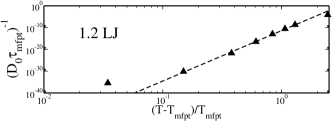
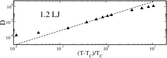
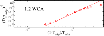
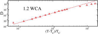
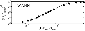
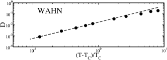
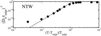
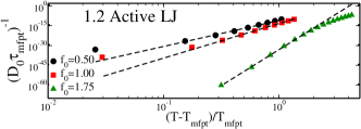
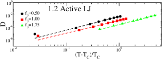
In Fig.1 we show some representative plots of the temperature dependence of the inverse mean first passage time for different model systems system_details_new . We also plot the corresponding diffusion (D) values for these systems. We find that for each of these systems the shows a power law divergence and can predict a transition temperature () of the respective systems given in Table 1. Note that not only the temperature , is similar to the critical temperature obtained from the MCT power law behaviour of diffusion, (also given in Table 1), but also the temperature regime over which shows linearity is similar to that of the diffusion (Fig.1)/ relaxation time manoj_unravel .

| KALJ | KAWCA | Active LJ | NTW | WAHN | |||||||
|---|---|---|---|---|---|---|---|---|---|---|---|
| 1.2 | 1.4 | 1.6 | 1.2 | 1.4 | 1.6 | ||||||
| 0.428 | 0.94 | 1.757 | 0.283 | 0.824 | 1.691 | 0.38 | 0.335 | 0.196 | 0.308 | 0.566 | |
| 0.022 | 0.029 | 0.042 | 0.005 | 0.04 | 0.018 | 0.004 | 0.006 | 0.013 | 0.012 | 0.013 | |
| 0.435 | 0.93 | 1.76 | 0.28 | 0.81 | 1.69 | 0.39 | 0.34 | 0.19 | 0.31 | 0.56 | |
| 0.887 | 1.868 | 3.528 | 0.76 | 1.771 | 3.33 | 0.768 | 0.761 | 0.747 | 0.464 | 0.87 | |
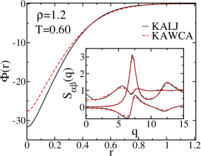
To show that the present analysis is sensitive to small changes in structure, we compare the results of KALJ and KAWCA systems at . In Fig.2 we plot which is used to calculate (via Eq.(5)) and show that although the structures are similar, the one body potentials are different. This difference is enough to predict the difference in (see Table 1). This observation is similar to that presented in an earlier study, where we have shown that although the radial distribution functions are quite similar, the pair configurational entropy () for these systems are different atreyee-Sc2 . Thus the temperature at which the vanishes are also different.
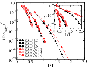
Further we show that this method of mean first passage time calculation can also predict the density effect. In Fig.3 we plot the for KALJ and KAWCA systems for three different densities. We also plot the following diffusion coefficients in the inset. Note that the show similar behaviour as the diffusion coefficients. At low density the values for the two systems are apart and at high density they overlap.
Next we show that we can derive the standard microscopic MCT equation from our present formalism. Eq.(3) when expressed in terms of the fluctuation of density, (, where is the averaged density of the system) and is replaced in terms of , can be written as,
| (6) |
Next in Eq.(6) we use the expressionramakrishnan-yossuf of . After taking the functional derivative of excess free energy and then the gradient of it, we can write Eq.(6) as,
| (7) |
Eq.(7) is the Langevin equation for the density field. Following Kawasaki’s arguments, this equation can be converted into standard MCT equation kawasaki ; snandi . The last non-linear term on the right hand side can be identified as the fluctuating force. In non-Markovian limit applying fluctuation dissipation relation (FDR) kawasaki , the friction can be replaced by short time part of friction and a memory function . Thus we can rewrite Eq.(7) as,
| (8) |
where is the new thermal noise and (see SI). Here we use Gaussian decoupling and Wick’s theorem to treat the four-point correlation function. We can write a mode coupling theory equation in the over-damped limit for density-density correlation .
| (9) |
In Table 1 we present the transition temperatures predicted by Eq.(9). We find that for all the systems . This higher value of can be connected to the approximations used to arrive from Eq.(3) to Eq.(9). In a recent work we have also shown that the form of the vertex function in the theory which depends on the structure factor might also be responsible for this premature divergence manoj_unravel .
In the present work in analogy with mean-field descriptions of spin systems, we reduce the dynamics of the N-interacting particle system given by Fokker-Planck equation to that of N-non-interacting particle system in an effective external potential where the latter provides the effect of the interaction only at the two body level. Thus in our formalism by construction we do not have any effect of correlation beyond two body. We then obtain the mean first passage time, which now depends only on the structure of the liquid. The temperature dependence of it, can predict a transition temperature which is similar to . Thus we conclude that the information of the MCT transition temperature is embedded in the pair structure of the liquid and it is the mean field transition temperature. In an earlier work, we have shown that the pair configurational entropy () vanishes at atreyee-Sc2 . At infinite dimension should be the total configurational entropy and the temperature at which it vanishes should be the Kauzmann temperature. Also for those systems the Kauzmann temperature and the mean field transition temperature should be similar. Thus our earlier result of vanishing at is consistent and similar to the present finding. In this present work we further show that starting from the same Fokker-Planck equation we can also derive the microscopic MCT equation. However the transition temperature predicted by the microscopic MCT is much higher than the value. Thus the break down of microscopic MCT in predicting the transition temperature, can be connected to the Gaussian decoupling approximation. However our present formalism although predicts the correct transition temperature, unlike the microscopic MCT the power law exponent is not universal. Also note that this present method of deriving the transition temperature is intimately connected to the structure of the liquid. Thus for systems like pinned particles, as the structure remains same, this theory will not be able to predict different transition temperatures for different pinning densities.
References
- (1) J. G. Kirkwood and E. M. Boggs, J. Chem. Phys. 10, 394 (1942).
- (2) R. E. Nettleton and M. S. Green, J. Chem. Phys. 29, 1365 (1958).
- (3) H. J. Raveché, J. Chem. Phys. 55, 2242 (1971).
- (4) D. C. Wallace, J. Chem. Phys. 87, 2282 (1987).
- (5) A. Banerjee, S. Sengupta, S. Sastry, and S. M. Bhattacharyya, Phys. Rev. Lett. 113, 225701 (2014).
- (6) M. K. Nandi, A. Banerjee, S. Sengupta, S. Sastry, and S. M. Bhattacharyya, J Chem. Phys. 143, 174504 (2015).
- (7) The values for WAHN and NTW model have been found to be similar with which will be reported in future communication .
- (8) E. Flenner and G. Szamel, Phys. Rev. E 72, 031508 (2005).
- (9) K. Kim and S. Saito, J. Chem. Phys. 138, 12A506 (2013).
- (10) W. Du et al., Phys. Rev. E 49, 2192 (1994).
- (11) P. Lunkenheimer, A. Pimenov, and A. Loidl, Phys. Rev. Lett. 78, 2995 (1997).
- (12) W. Götze, J. Phys.Condens. Matter 11, A1 (1999).
- (13) L. M. C. Janssen, P. Mayer, and D. R. Reichman, J. Stat. Mech. 2016, 054049 (2016).
- (14) T. R. Kirkpatrick, D. Thirumalai, and P. G. Wolynes, Phys. Rev. A 40, 1045 (1989).
- (15) A. Cavagna, EPL 53, 490 (2001).
- (16) S. Mossa et al., Phys. Rev. E 65, 041205 (2002).
- (17) L. Angelani, R. Di Leonardo, G. Ruocco, A. Scala, and F. Sciortino, J. Chem. Phys. 116, 10297 (2002).
- (18) S. M. Bhattacharyya, B. Bagchi, and P. G. Wolynes, PNAS 105, 16077 (2008).
- (19) Y. Brumer and D. R. Reichman, Phys. Rev. E 69, 041202 (2004).
- (20) T. R. Kirkpatrick and P. G. Wolynes, Phys. Rev. A 35, 3072 (1987).
- (21) K. S. Schweizer, J. chem. phys. 123, 244501 (2005).
- (22) H. Risken, The Fokker-Planck Equation (Springer 1989).
- (23) R. Evans, Adv. Phys. 28, 143 (1979).
- (24) T. Ramakrishnan and M. Yussouff, Phys. Rev. B 19, 2775 (1979).
- (25) R. Zwanzig, PNAS 85, 2029 (1988).
- (26) The systems studied are Kob Andersen model with Lennard-Jones (KALJ), see W. Kob and H. C. Andersen, Phys. Rev. E 51, 4626 (1995) and its repulsive counterpart Weeks-Chandeler-Andersen potential (KAWCA), see J. D. Weeks, D. Chandler, and H. C. Andersen, J. Chem. Phys. 54, 5237 (1971) , Wahnström model (WAHN), see G. Wahnström, Phys. Rev. A 44, 3752 (1991), network forming model (NTW), see D. Coslovich and G. Pastore, J. Phys. Condens. Matter 21, 285107 (2009) and the active systems, see R. Mandal, P. J. Bhuyan, M. Rao, and C. Dasgupta, Soft Matter 12, 6268 (2016). Lengths, temperatures, and times are given in units of , , respectively. Although the analytical calculations are done for mono-atomic systems, note that the numerical calculations are done for binary systems (see SI) .
- (27) L. Berthier and G. Tarjus, Phys. Rev. E 82, 031502 (2010).
- (28) values are obtained by fitting the diffusion values for active systems in mode coupling theory power law fit. The exponents are 2.31, 2.27 and 2.10 for activity 0.50, 1.00 and 1.75 respectively. The data is similar to that given in R. Mandal, P. J. Bhuyan, M. Rao, and C. Dasgupta, Soft Matter 12, 6268 (2016) and obtained through private communication .
- (29) G. Wahnström, Phys. Rev. A 44, 3752 (1991).
- (30) L. Berthier, G. Biroli, D. Coslovich, W. Kob, and C. Toninelli, Phys. Rev. E 86, 031502 (2012).
- (31) A. Banerjee, M. K. Nandi, S. Sastry, and S. M. Bhattacharyya, J. Chem. Phys. 145, 034502 (2016).
- (32) K. Kawasaki, J. stat. phys. 110, 1249 (2003).
- (33) S. Nandi, Ph.D. Thesis (Indian Institute of Science, 2012).