Training Quantized Nets: A Deeper Understanding

Hao Li1 , Soham De1footnotemark:  , Zheng Xu1, Christoph Studer2, Hanan Samet1, Tom Goldstein1
1Department of Computer Science, University of Maryland, College Park
2School of Electrical and Computer Engineering, Cornell University
{haoli,sohamde,xuzh,hjs,tomg}@cs.umd.edu, studer@cornell.edu
Equal contribution. Author ordering determined by a cryptographically secure random number generator.
Abstract

Currently, deep neural networks are deployed on low-power portable devices by first training a full-precision model using powerful hardware, and then deriving a corresponding low-precision model for efficient inference on such systems. However, training models directly with coarsely quantized weights is a key step towards learning on embedded platforms that have limited computing resources, memory capacity, and power consumption. Numerous recent publications have studied methods for training quantized networks, but these studies have mostly been empirical. In this work, we investigate training methods for quantized neural networks from a theoretical viewpoint. We first explore accuracy guarantees for training methods under convexity assumptions. We then look at the behavior of these algorithms for non-convex problems, and show that training algorithms that exploit high-precision representations have an important greedy search phase that purely quantized training methods lack, which explains the difficulty of training using low-precision arithmetic.

1 Introduction

Deep neural networks are an integral part of state-of-the-art computer vision and natural language processing systems. Because of their high memory requirements and computational complexity, networks are usually trained using powerful hardware. There is an increasing interest in training and deploying neural networks directly on battery-powered devices, such as cell phones or other platforms. Such low-power embedded systems are memory and power limited, and in some cases lack basic support for floating-point arithmetic.

To make neural nets practical on embedded systems, many researchers have focused on training nets with coarsely quantized weights. For example, weights may be constrained to take on integer/binary values, or may be represented using low-precision (8 bits or less) fixed-point numbers. Quantized nets offer the potential of superior memory and computation efficiency, while achieving performance that is competitive with state-of-the-art high-precision nets. Quantized weights can dramatically reduce memory size and access bandwidth, increase power efficiency, exploit hardware-friendly bitwise operations, and accelerate inference throughput [1, 2, 3].

Handling low-precision weights is difficult and motivates interest in new training methods. When learning rates are small, stochastic gradient methods make small updates to weight parameters. Binarization/discretization of weights after each training iteration “rounds off” these small updates and causes training to stagnate [1]. Thus, the naïve approach of quantizing weights using a rounding procedure yields poor results when weights are represented using a small number of bits. Other approaches include classical stochastic rounding methods [4], as well as schemes that combine full-precision floating-point weights with discrete rounding procedures [5]. While some of these schemes seem to work in practice, results in this area are largely experimental, and little work has been devoted to explaining the excellent performance of some methods, the poor performance of others, and the important differences in behavior between these methods.

Contributions

This paper studies quantized training methods from a theoretical perspective, with the goal of understanding the differences in behavior, and reasons for success or failure, of various methods. In particular, we present a convergence analysis showing that classical stochastic rounding (SR) methods [4] as well as newer and more powerful methods like BinaryConnect (BC) [5] are capable of solving convex discrete problems up to a level of accuracy that depends on the quantization level. We then address the issue of why algorithms that maintain floating-point representations, like BC, work so well, while fully quantized training methods like SR stall before training is complete. We show that the long-term behavior of BC has an important annealing property that is needed for non-convex optimization, while classical rounding methods lack this property.

2 Background and Related Work

The arithmetic operations of deep networks can be truncated down to 8-bit fixed-point without significant deterioration in inference performance [4, 6, 7, 8, 9]. The most extreme scenario of quantization is binarization, in which only 1-bit (two states) is used for weight representation [10, 5, 1, 3, 11, 12].

Previous work on obtaining a quantized neural network can be divided into two categories: quantizing pre-trained models with or without retraining [7, 13, 6, 14, 15], and training a quantized model from scratch  [4, 5, 3, 1, 16]. We focus on approaches that belong to the second category, as they can be used for both training and inference under constrained resources.

For training quantized NNs from scratch, many authors suggest maintaining a high-precision floating point copy of the weights while feeding quantized weights into backprop [5, 11, 3, 16], which results in good empirical performance. There are limitations in using such methods on low-power devices, however, where floating-point arithmetic is not always available or not desirable. Another widely used solution using only low-precision weights is stochastic rounding [17, 4]. Experiments show that networks using 16-bit fixed-point representations with stochastic rounding can deliver results nearly identical to 32-bit floating-point computations [4], while lowering the precision down to 3-bit fixed-point often results in a significant performance degradation [18]. Bayesian learning has also been applied to train binary networks [19, 20]. A more comprehensive review can be found in [3].

3 Training Quantized Neural Nets

We consider empirical risk minimization problems of the form:

minw𝒲F(w):=1mi=1mfi(w),assignsubscript𝑤𝒲𝐹𝑤1𝑚superscriptsubscript𝑖1𝑚subscript𝑓𝑖𝑤\displaystyle\min_{w\in\mathcal{W}}F(w):=\frac{1}{m}\sum_{i=1}^{m}f_{i}(w), (1)

where the objective function decomposes into a sum over many functions fi:d:subscript𝑓𝑖superscript𝑑f_{i}:\mathbb{R}^{d}\rightarrow\mathbb{R}. Neural networks have objective functions of this form where each fisubscript𝑓𝑖f_{i} is a non-convex loss function. When floating-point representations are available, the standard method for training neural networks is stochastic gradient descent (SGD), which on each iteration selects a function f~~𝑓\tilde{f} randomly from {f1,f2,,fm}subscript𝑓1subscript𝑓2subscript𝑓𝑚\{f_{1},f_{2},\dots,f_{m}\}, and then computes

SGD: wt+1=wtαtf~(wt),SGD: superscript𝑤𝑡1superscript𝑤𝑡subscript𝛼𝑡~𝑓superscript𝑤𝑡\displaystyle\text{SGD: }\,\,w^{t+1}=w^{t}-\alpha_{t}\nabla\tilde{f}(w^{t}), (2)

for some learning rate αtsubscript𝛼𝑡\alpha_{t}. In this paper, we consider the problem of training convolutional neural networks (CNNs). Convolutions are computationally expensive; low precision weights can be used to accelerate them by replacing expensive multiplications with efficient addition and subtraction operations [3, 9] or bitwise operations [11, 16].

To train networks using a low-precision representation of the weights, a quantization function Q()𝑄Q(\cdot) is needed to convert a real-valued number w𝑤w into a quantized/rounded version w^=Q(w)^𝑤𝑄𝑤\hat{w}=Q(w). We use the same notation for quantizing vectors, where we assume Q𝑄Q acts on each dimension of the vector. Different quantized optimization routines can be defined by selecting different quantizers, and also by selecting when quantization happens during optimization. The common options are:

Deterministic Rounding (R)

A basic uniform or deterministic quantization function snaps a floating point value to the closest quantized value as:

Qd(w)=sign(w)Δ|w|Δ+12,subscript𝑄𝑑𝑤sign𝑤Δ𝑤Δ12\displaystyle Q_{d}(w)=\text{sign}(w)\cdot\Delta\cdot\!\left\lfloor\frac{|w|}{\Delta}+\frac{1}{2}\right\rfloor, (3)

where ΔΔ\Delta denotes the quantization step or resolution, i.e., the smallest positive number that is representable. One exception to this definition is when we consider binary weights, where all weights are constrained to have two values w{1,1}𝑤11w\in\{-1,1\} and uniform rounding becomes Qd(w)=sign(w).subscript𝑄𝑑𝑤sign𝑤Q_{d}(w)=\operatorname*{sign}(w).

The deterministic rounding SGD maintains quantized weights with updates of the form:

Deterministic Rounding: wbt+1=Qd(wbtαtf~(wbt)),Deterministic Rounding: superscriptsubscript𝑤𝑏𝑡1subscript𝑄𝑑superscriptsubscript𝑤𝑏𝑡subscript𝛼𝑡~𝑓superscriptsubscript𝑤𝑏𝑡\displaystyle\text{Deterministic Rounding: }\,\,w_{b}^{t+1}=Q_{d}\big{(}w_{b}^{t}-\alpha_{t}\nabla\tilde{f}(w_{b}^{t})\big{)}, (4)

where wbsubscript𝑤𝑏w_{b} denotes the low-precision weights, which are quantized using Qdsubscript𝑄𝑑Q_{d} immediately after applying the gradient descent update. If gradient updates are significantly smaller than the quantization step, this method loses gradient information and weights may never be modified from their starting values.

Stochastic Rounding (SR)

The quantization function for stochastic rounding is defined as:

Qs(w)=Δ{wΔ+1for pwΔwΔ,wΔotherwise,subscript𝑄𝑠𝑤Δcases𝑤Δ1for 𝑝𝑤Δ𝑤Δ𝑤Δotherwise,Q_{s}(w)=\Delta\cdot\begin{cases}\lfloor\frac{w}{\Delta}\rfloor+1&\text{for }p\leq\frac{w}{\Delta}-\lfloor\frac{w}{\Delta}\rfloor,\\ \lfloor\frac{w}{\Delta}\rfloor&\text{otherwise,}\end{cases} (5)

where p[0,1]𝑝01p\in[0,1] is produced by a uniform random number generator. This operator is non-deterministic, and rounds its argument up with probability w/Δw/Δ,𝑤Δ𝑤Δw/\Delta-\lfloor w/\Delta\rfloor, and down otherwise. This quantizer satisfies the important property 𝔼[Qs(w)]=w𝔼delimited-[]subscript𝑄𝑠𝑤𝑤\mathbb{E}[Q_{s}(w)]=w. Similar to the deterministic rounding method, the SR optimization method also maintains quantized weights with updates of the form:

Stochastic Rounding: wbt+1=Qs(wbtαtf~(wbt)).Stochastic Rounding: superscriptsubscript𝑤𝑏𝑡1subscript𝑄𝑠superscriptsubscript𝑤𝑏𝑡subscript𝛼𝑡~𝑓superscriptsubscript𝑤𝑏𝑡\displaystyle\text{Stochastic Rounding: }\,\,w_{b}^{t+1}=Q_{s}\big{(}w_{b}^{t}-\alpha_{t}\nabla\tilde{f}(w_{b}^{t})\big{)}. (6)

BinaryConnect (BC)

The BinaryConnect algorithm [5] accumulates gradient updates using a full-precision buffer wr,subscript𝑤𝑟w_{r}, and quantizes weights just before gradient computations as follows.

BinaryConnect: wrt+1=wrtαtf~(Q(wrt)).BinaryConnect: superscriptsubscript𝑤𝑟𝑡1superscriptsubscript𝑤𝑟𝑡subscript𝛼𝑡~𝑓𝑄superscriptsubscript𝑤𝑟𝑡\displaystyle\text{BinaryConnect: }\,\,w_{r}^{t+1}=w_{r}^{t}-\alpha_{t}\nabla\tilde{f}\big{(}Q(w_{r}^{t})\big{)}. (7)

Either stochastic rounding Qssubscript𝑄𝑠Q_{s} or deterministic rounding Qdsubscript𝑄𝑑Q_{d} can be used for quantizing the weights wrsubscript𝑤𝑟w_{r}, but in practice, Qdsubscript𝑄𝑑Q_{d} is the common choice. The original BinaryConnect paper constrains the low-precision weights to be {1,1}11\{-1,1\}, which can be generalized to {Δ,Δ}ΔΔ\{-\Delta,\Delta\}. A more recent method, Binary-Weights-Net (BWN) [3], allows different filters to have different scales for quantization, which often results in better performance on large datasets.

Notation

For the rest of the paper, we use Q𝑄Q to denote both Qssubscript𝑄𝑠Q_{s} and Qdsubscript𝑄𝑑Q_{d} unless the situation requires this to be distinguished. We also drop the subscripts on wrsubscript𝑤𝑟w_{r} and wbsubscript𝑤𝑏w_{b}, and simply write w.𝑤w.

4 Convergence Analysis

We now present convergence guarantees for the Stochastic Rounding (SR) and BinaryConnect (BC) algorithms, with updates of the form (6) and (7), respectively. For the purposes of deriving theoretical guarantees, we assume each fisubscript𝑓𝑖f_{i} in (1) is differentiable and convex, and the domain 𝒲𝒲\mathcal{W} is convex and has dimension d𝑑d. We consider both the case where F𝐹F is μ𝜇\mu-strongly convex: F(w),wwF(w)F(w)μ2ww2𝐹superscript𝑤𝑤superscript𝑤𝐹𝑤𝐹superscript𝑤𝜇2superscriptnorm𝑤superscript𝑤2\langle\nabla F(w^{\prime}),w-w^{\prime}\rangle\leq F(w)-F(w^{\prime})-\frac{\mu}{2}\|w-w^{\prime}\|^{2}, as well as where F𝐹F is weakly convex. We also assume the (stochastic) gradients are bounded: 𝔼f~(wt)2G2𝔼superscriptnorm~𝑓superscript𝑤𝑡2superscript𝐺2\mathbb{E}\|\nabla\tilde{f}(w^{t})\|^{2}\leq G^{2}. Some results below also assume the domain of the problem is finite. In this case, the rounding algorithm clips values that leave the domain. For example, in the binary case, rounding returns bounded values in {1,1}.11\{-1,1\}.

4.1 Convergence of Stochastic Rounding (SR)

We can rewrite the update rule (6) as:

wt+1=wtαtf~(wt)+rt,superscript𝑤𝑡1superscript𝑤𝑡subscript𝛼𝑡~𝑓superscript𝑤𝑡superscript𝑟𝑡\displaystyle w^{t+1}=w^{t}-\alpha_{t}\nabla\tilde{f}(w^{t})+r^{t},

where rt=Qs(wtαtf~(wt))wt+αtf~(wt)superscript𝑟𝑡subscript𝑄𝑠superscript𝑤𝑡subscript𝛼𝑡~𝑓superscript𝑤𝑡superscript𝑤𝑡subscript𝛼𝑡~𝑓superscript𝑤𝑡r^{t}=Q_{s}(w^{t}-\alpha_{t}\nabla\tilde{f}(w^{t}))-w^{t}+\alpha_{t}\nabla\tilde{f}(w^{t}) denotes the quantization error on the t𝑡t-th iteration. We want to bound this error in expectation. To this end, we present the following lemma.

Lemma 1.

The stochastic rounding error rtsuperscript𝑟𝑡r^{t} on each iteration can be bounded, in expectation, as:

𝔼rt2dΔαtG,𝔼superscriptnormsuperscript𝑟𝑡2𝑑Δsubscript𝛼𝑡𝐺\displaystyle\mathbb{E}\big{\|}r^{t}\big{\|}^{2}\leq\sqrt{d}\Delta\alpha_{t}G,

where d𝑑d denotes the dimension of w𝑤w.

Proofs for all theoretical results are presented in the Appendices. From Lemma 1, we see that the rounding error per step decreases as the learning rate αtsubscript𝛼𝑡\alpha_{t} decreases. This is intuitive since the probability of an entry in wt+1superscript𝑤𝑡1w^{t+1} differing from wtsuperscript𝑤𝑡w^{t} is small when the gradient update is small relative to ΔΔ\Delta. Using the above lemma, we now present convergence rate results for Stochastic Rounding (SR) in both the strongly-convex case and the non-strongly convex case. Our error estimates are ergodic, i.e., they are in terms of w¯T=1Tt=1Twtsuperscript¯𝑤𝑇1𝑇superscriptsubscript𝑡1𝑇superscript𝑤𝑡\bar{w}^{T}=\frac{1}{T}\sum_{t=1}^{T}w^{t}, the average of the iterates.

Theorem 1.

Assume that F𝐹F is μ𝜇\mu-strongly convex and the learning rates are given by αt=1μ(t+1)subscript𝛼𝑡1𝜇𝑡1\alpha_{t}=\frac{1}{\mu(t+1)}. Consider the SR algorithm with updates of the form (6). Then, we have:

𝔼[F(w¯T)F(w)](1+log(T+1))G22μT+dΔG2,𝔼delimited-[]𝐹superscript¯𝑤𝑇𝐹superscript𝑤1𝑇1superscript𝐺22𝜇𝑇𝑑Δ𝐺2\displaystyle\mathbb{E}[F(\bar{w}^{T})-F(w^{\star})]\leq\frac{(1+\log(T+1))G^{2}}{2\mu T}+\frac{\sqrt{d}\Delta G}{2},

where w=argminwF(w)superscript𝑤subscriptargmin𝑤𝐹𝑤w^{\star}=\operatorname*{arg\,min}_{w}F(w).

Theorem 2.

Assume the domain has finite diameter D,𝐷D, and learning rates are given by αt=ctsubscript𝛼𝑡𝑐𝑡\alpha_{t}=\frac{c}{\sqrt{t}}, for a constant c𝑐c. Consider the SR algorithm with updates of the form (6). Then, we have:

𝔼[F(w¯T)F(w)]1cTD2+T+12TcG2+dΔG2.𝔼delimited-[]𝐹superscript¯𝑤𝑇𝐹superscript𝑤1𝑐𝑇superscript𝐷2𝑇12𝑇𝑐superscript𝐺2𝑑Δ𝐺2\displaystyle\mathbb{E}[F(\bar{w}^{T})-F(w^{\star})]\leq\frac{1}{c\sqrt{T}}D^{2}+\frac{\sqrt{T+1}}{2T}cG^{2}+\frac{\sqrt{d}\Delta G}{2}.

We see that in both cases, SR converges until it reaches an “accuracy floor.” As the quantization becomes more fine grained, our theory predicts that the accuracy of SR approaches that of high-precision floating point at a rate linear in Δ.Δ\Delta. This extra term caused by the discretization is unavoidable since this method maintains quantized weights.

4.2 Convergence of Binary Connect (BC)

When analyzing the BC algorithm, we assume that the Hessian satisfies the Lipschitz bound: 2fi(x)2fi(y)L2xynormsuperscript2subscript𝑓𝑖𝑥superscript2subscript𝑓𝑖𝑦subscript𝐿2norm𝑥𝑦\|\nabla^{2}f_{i}(x)-\nabla^{2}f_{i}(y)\|\leq L_{2}\|x-y\| for some L20.subscript𝐿20L_{2}\geq 0. While this is a slightly non-standard assumption, we will see that it enables us to gain better insights into the behavior of the algorithm.

The results here hold for both stochastic and uniform rounding. In this case, the quantization error r𝑟r does not approach 0 as in SR-SGD. Nonetheless, the effect of this rounding error diminishes with shrinking αtsubscript𝛼𝑡\alpha_{t} because αtsubscript𝛼𝑡\alpha_{t} multiplies the gradient update, and thus implicitly the rounding error as well.

Theorem 3.

Assume F𝐹F is L𝐿L-Lipschitz smooth, the domain has finite diameter D,𝐷D, and learning rates are given by αt=ctsubscript𝛼𝑡𝑐𝑡\alpha_{t}=\frac{c}{\sqrt{t}}. Consider the BC-SGD algorithm with updates of the form (7). Then, we have:

𝔼[F(w¯T)F(w)]12cTD2+T+12TcG2+dΔLD.𝔼delimited-[]𝐹superscript¯𝑤𝑇𝐹superscript𝑤12𝑐𝑇superscript𝐷2𝑇12𝑇𝑐superscript𝐺2𝑑Δ𝐿𝐷\displaystyle\mathbb{E}[F(\bar{w}^{T})-F(w^{\star})]\leq\frac{1}{2c\sqrt{T}}D^{2}+\frac{\sqrt{T+1}}{2T}cG^{2}+\sqrt{d}\Delta LD.

As with SR, BC can only converge up to an error floor. So far this looks a lot like the convergence guarantees for SR. However, things change when we assume strong convexity and bounded Hessian.

Theorem 4.

Assume that F𝐹F is μ𝜇\mu-strongly convex and the learning rates are given by αt=1μ(t+1)subscript𝛼𝑡1𝜇𝑡1\alpha_{t}=\frac{1}{\mu(t+1)}. Consider the BC algorithm with updates of the form (7). Then we have:

𝔼[F(w¯T)F(w)](1+log(T+1))G22μT+DL2dΔ2.𝔼delimited-[]𝐹superscript¯𝑤𝑇𝐹superscript𝑤1𝑇1superscript𝐺22𝜇𝑇𝐷subscript𝐿2𝑑Δ2\displaystyle\mathbb{E}[F(\bar{w}^{T})-F(w^{\star})]\leq\frac{(1+\log(T+1))G^{2}}{2\mu T}+\frac{DL_{2}\sqrt{d}\Delta}{2}.

Now, the error floor is determined by both ΔΔ\Delta and L2.subscript𝐿2L_{2}. For a quadratic least-squares problem, the gradient of F𝐹F is linear and the Hessian is constant. Thus, L2=0subscript𝐿20L_{2}=0 and we get the following corollary.

Corollary 1.

Assume that F𝐹F is quadratic and the learning rates are given by αt=1μ(t+1)subscript𝛼𝑡1𝜇𝑡1\alpha_{t}=\frac{1}{\mu(t+1)}. The BC algorithm with updates of the form (7) yields

𝔼[F(w¯T)F(w)](1+log(T+1))G22μT.𝔼delimited-[]𝐹superscript¯𝑤𝑇𝐹superscript𝑤1𝑇1superscript𝐺22𝜇𝑇\displaystyle\mathbb{E}[F(\bar{w}^{T})-F(w^{\star})]\leq\frac{(1+\log(T+1))G^{2}}{2\mu T}.

We see that the real-valued weights accumulated in BC can converge to the true minimizer of quadratic losses. Furthermore, this suggests that, when the function behaves like a quadratic on the distance scale Δ,Δ\Delta, one would expect BC to perform fundamentally better than SR. While this may seem like a restrictive condition, there is evidence that even non-convex neural networks become well approximated as a quadratic in the later stages of optimization within a neighborhood of a local minimum [21].

Note, our convergence results on BC are for wrsubscript𝑤𝑟w_{r} instead of wb,subscript𝑤𝑏w_{b}, and these measures of convergence are not directly comparable. It is not possible to bound wbsubscript𝑤𝑏w_{b} when BC is used, as the values of wbsubscript𝑤𝑏w_{b} may not converge in the usual sense (e.g., in the +/-1 binary case wrsubscript𝑤𝑟w_{r} might converge to 0, in which case arbitrarily small perturbations to wrsubscript𝑤𝑟w_{r} might send wbsubscript𝑤𝑏w_{b} to +1 or -1).

5 What About Non-Convex Problems?

The global convergence results presented above for convex problems show that, in general, both the SR and BC algorithms converge to within 𝒪(Δ)𝒪Δ\mathcal{O}(\Delta) accuracy of the minimizer (in expected value). However, these results do not explain the large differences between these methods when applied to non-convex neural nets. We now study how the long-term behavior of SR differs from BC. Note that this section makes no convexity assumptions, and the proposed theoretical results are directly applicable to neural networks.

Typical (continuous-valued) SGD methods have an important exploration-exploitation tradeoff. When the learning rate is large, the algorithm explores by moving quickly between states. Exploitation happens when the learning rate is small. In this case, noise averaging causes the algorithm more greedily pursues local minimizers with lower loss values. Thus, the distribution of iterates produced by the algorithm becomes increasingly concentrated near minimizers as the learning rate vanishes (see, e.g., the large-deviation estimates in [22]). BC maintains this property as well—indeed, we saw in Corollary 1 a class of problems for which the iterates concentrate on the minimizer for small αt.subscript𝛼𝑡\alpha_{t}.

In this section, we show that the SR method lacks this important tradeoff: as the stepsize gets small and the algorithm slows down, the quality of the iterates produced by the algorithm does not improve, and the algorithm does not become progressively more likely to produce low-loss iterates. This behavior is illustrated in Figures 1 and 2.

To understand this problem conceptually, consider the simple case of a one-variable optimization problem starting at x0=0superscript𝑥00x^{0}=0 with Δ=1Δ1\Delta=1 (Figure 1). On each iteration, the algorithm computes a stochastic approximation f~~𝑓\nabla\tilde{f} of the gradient by sampling from a distribution, which we call p.𝑝p. This gradient is then multiplied by the stepsize to get αf~.𝛼~𝑓\alpha\nabla\tilde{f}. The probability of moving to the right (or left) is then roughly proportional to the magnitude of αf~.𝛼~𝑓\alpha\nabla\tilde{f}. Note the random variable αf~𝛼~𝑓\alpha\nabla\tilde{f} has distribution pα(z)=α1p(z/α).subscript𝑝𝛼𝑧superscript𝛼1𝑝𝑧𝛼p_{\alpha}(z)=\alpha^{-1}p(z/\alpha).

Refer to caption
Figure 1: The SR method starts at some location x𝑥x (in this case 00), adds a perturbation to x,𝑥x, and then rounds. As the learning rate α𝛼\alpha gets smaller, the distribution of the perturbation gets “squished” near the origin, making the algorithm less likely to move. The “squishing” effect is the same for the part of the distribution lying to the left and to the right of x,𝑥x, and so it does not effect the relative probability of moving left or right.

Now, suppose that α𝛼\alpha is small enough that we can neglect the tails of pα(z)subscript𝑝𝛼𝑧p_{\alpha}(z) that lie outside the interval [1,1].11[-1,1]. The probability of transitioning from x0=0superscript𝑥00x^{0}=0 to x1=1superscript𝑥11x^{1}=1 using stochastic rounding, denoted by Tα(0,1),subscript𝑇𝛼01T_{\alpha}(0,1), is then

Tα(0,1)01zpα(z)𝑑z=1α01zp(z/α)𝑑z=α01/αp(x)x𝑑xα0p(x)x𝑑x,subscript𝑇𝛼01superscriptsubscript01𝑧subscript𝑝𝛼𝑧differential-d𝑧1𝛼superscriptsubscript01𝑧𝑝𝑧𝛼differential-d𝑧𝛼superscriptsubscript01𝛼𝑝𝑥𝑥differential-d𝑥𝛼superscriptsubscript0𝑝𝑥𝑥differential-d𝑥T_{\alpha}(0,1)\approx\int_{0}^{1}zp_{\alpha}(z)dz=\frac{1}{\alpha}\int_{0}^{1}zp(z/\alpha)\,dz=\alpha\int_{0}^{1/\alpha}p(x)x\,dx\approx\alpha\int_{0}^{\infty}p(x)x\,dx,

where the first approximation is because we neglected the unlikely case that αf~>1,𝛼~𝑓1\alpha\nabla\tilde{f}>1, and the second approximation appears because we added a small tail probability to the estimate. These approximations get more accurate for small α.𝛼\alpha. We see that, assuming the tails of p𝑝p are “light” enough, we have Tα(0,1)α0p(x)x𝑑xsimilar-tosubscript𝑇𝛼01𝛼superscriptsubscript0𝑝𝑥𝑥differential-d𝑥T_{\alpha}(0,1)\sim\alpha\int_{0}^{\infty}p(x)x\,dx as α0.𝛼0\alpha\to 0. Similarly, Tα(0,1)α0p(x)x𝑑xsimilar-tosubscript𝑇𝛼01𝛼superscriptsubscript0𝑝𝑥𝑥differential-d𝑥T_{\alpha}(0,-1)\sim\alpha\int_{-\infty}^{0}p(x)x\,dx as α0.𝛼0\alpha\to 0.

What does this observation mean for the behavior of SR? First of all, the probability of leaving x0superscript𝑥0x^{0} on an iteration is

Tα(0,1)+Tα(0,1)α[0p(x)x𝑑x+0p(x)x𝑑x],subscript𝑇𝛼01subscript𝑇𝛼01𝛼delimited-[]superscriptsubscript0𝑝𝑥𝑥differential-d𝑥superscriptsubscript0𝑝𝑥𝑥differential-d𝑥T_{\alpha}(0,-1)+T_{\alpha}(0,1)\approx\alpha\left[\int_{0}^{\infty}p(x)x\,dx+\int_{-\infty}^{0}p(x)x\,dx\right],

which vanishes for small α.𝛼\alpha. This means the algorithm slows down as the learning rate drops off, which is not surprising. However, the conditional probability of ending up at x1=1superscript𝑥11x^{1}=1 given that the algorithm did leave x0superscript𝑥0x^{0} is

Tα(0,1|x1x0)Tα(0,1)Tα(0,1)+Tα(0,1)=0p(x)x𝑑x0p(x)x𝑑x+0p(x)x𝑑x,subscript𝑇𝛼0conditional1superscript𝑥1superscript𝑥0subscript𝑇𝛼01subscript𝑇𝛼01subscript𝑇𝛼01superscriptsubscript0𝑝𝑥𝑥differential-d𝑥superscriptsubscript0𝑝𝑥𝑥differential-d𝑥superscriptsubscript0𝑝𝑥𝑥differential-d𝑥T_{\alpha}(0,1|x^{1}\neq x^{0})\approx\frac{T_{\alpha}(0,1)}{T_{\alpha}(0,-1)+T_{\alpha}(0,1)}=\frac{\int_{0}^{\infty}p(x)x\,dx}{\int_{-\infty}^{0}p(x)x\,dx+\int_{0}^{\infty}p(x)x\,dx}\,,

which does not depend on α.𝛼\alpha. In other words, provided α𝛼\alpha is small, SR, on average, makes the same decisions/transitions with learning rate α𝛼\alpha as it does with learning rate α/10𝛼10\alpha/10; it just takes 10 times longer to make those decisions when α/10𝛼10\alpha/10 is used. In this situation, there is no exploitation benefit in decreasing α.𝛼\alpha.

5.1 Toy Problem

Refer to caption Refer to caption Refer to caption Refer to caption Refer to caption
Refer to caption
(a) α=1.0𝛼1.0\alpha=1.0
Refer to caption
(b) α=0.1𝛼0.1\alpha=0.1
Refer to caption
(c) α=0.01𝛼0.01\alpha=0.01
Refer to caption
(d) α=0.001𝛼0.001\alpha=0.001
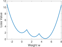
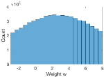
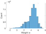
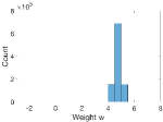
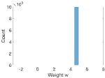
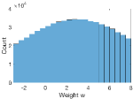
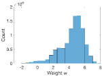
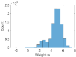
Figure 2: Effect of shrinking the learning rate in SR vs BC on a toy problem. The left figure plots the objective function (8). Histograms plot the distribution of the quantized weights over 106superscript10610^{6} iterations. The top row of plots correspond to BC, while the bottom row is SR, for different learning rates α𝛼\alpha. As the learning rate α𝛼\alpha shrinks, the BC distribution concentrates on a minimizer, while the SR distribution stagnates.

To gain more intuition about the effect of shrinking the learning rate in SR vs BC, consider the following simple 1-dimensional non-convex problem:

minwf(w):={w2+2,if w<1,(w2.5)2+0.75,if 1w<3.5,(w4.75)2+0.19,if w3.5.assignsubscript𝑤𝑓𝑤casessuperscript𝑤22if 𝑤1otherwisesuperscript𝑤2.520.75if 1𝑤3.5otherwisesuperscript𝑤4.7520.19if 𝑤3.5otherwise\displaystyle\min_{w}f(w):=\begin{cases}w^{2}+2,\quad\quad\quad\quad\quad\,\,\,\,\,\,\,\text{if }w<1,\\ (w-2.5)^{2}+0.75,\quad\,\,\,\text{if }1\leq w<3.5,\\ (w-4.75)^{2}+0.19,\quad\text{if }w\geq 3.5.\end{cases} (8)

Figure 2 shows a plot of this loss function. To visualize the distribution of iterates, we initialize at w=4.0𝑤4.0w=4.0, and run SR and BC for 106superscript10610^{6} iterations using a quantization resolution of 0.5.

Figure 2 shows the distribution of the quantized weight parameters w𝑤w over the iterations when optimized with SR and BC for different learning rates α𝛼\alpha. As we shift from α=1𝛼1\alpha=1 to α=0.001,𝛼0.001\alpha=0.001, the distribution of BC iterates transitions from a wide/explorative distribution to a narrow distribution in which iterates aggressively concentrate on the minimizer. In contrast, the distribution produced by SR concentrates only slightly and then stagnates; the iterates are spread widely even when the learning rate is small.

5.2 Asymptotic Analysis of Stochastic Rounding

The above argument is intuitive, but also informal. To make these statements rigorous, we interpret the SR method as a Markov chain. On each iteration, SR starts at some state (iterate) x𝑥x, and moves to a new state y𝑦y with some transition probability Tα(x,y)subscript𝑇𝛼𝑥𝑦T_{\alpha}(x,y) that depends only on x𝑥x and the learning rate α.𝛼\alpha. For fixed α,𝛼\alpha, this is clearly a Markov process with transition matrix111Our analysis below does not require the state space to be finite, so Tα(x,y)subscript𝑇𝛼𝑥𝑦T_{\alpha}(x,y) may be a linear operator rather than a matrix. Nonetheless, we use the term “matrix” as it is standard. Tα(x,y)subscript𝑇𝛼𝑥𝑦T_{\alpha}(x,y).

The long-term behavior of this Markov process is determined by the stationary distribution of Tα(x,y)subscript𝑇𝛼𝑥𝑦T_{\alpha}(x,y). We show below that for small α,𝛼\alpha, the stationary distribution of Tα(x,y)subscript𝑇𝛼𝑥𝑦T_{\alpha}(x,y) is nearly invariant to α𝛼\alpha, and thus decreasing α𝛼\alpha below some threshold has virtually no effect on the long term behavior of the method. This happens because, as α𝛼\alpha shrinks, the relative transition probabilities remain the same (conditioned on the fact that the parameters change), even though the absolute probabilities decrease (see Figure 3). In this case, there is no exploitation benefit to decreasing α.𝛼\alpha.

ABC0.20.20.40.40.20.60.60.20.2
ABC0.10.10.20.20.10.30.80.60.6
Figure 3: Markov chain example with 3 states. In the right figure, we halved each transition probability for moving between states, with the remaining probability put on the self-loop. Notice that halving all the transition probabilities would not change the equilibrium distribution, and instead would only increase the mixing time of the Markov chain.
Theorem 5.

Let px,ksubscript𝑝𝑥𝑘p_{x,k} denote the probability distribution of the k𝑘kth entry in f~(x),~𝑓𝑥\nabla\tilde{f}(x), the stochastic gradient estimate at x.𝑥x. Assume there is a constant C1subscript𝐶1C_{1} such that for all x,𝑥x, k,𝑘k, and ν𝜈\nu we have νpx,k(z)𝑑zC1ν2,superscriptsubscript𝜈subscript𝑝𝑥𝑘𝑧differential-d𝑧subscript𝐶1superscript𝜈2\int_{\nu}^{\infty}p_{x,k}(z)\,dz\leq\frac{C_{1}}{\nu^{2}}, and some C2subscript𝐶2C_{2} such that both 0C2px,k(z)𝑑z>0superscriptsubscript0subscript𝐶2subscript𝑝𝑥𝑘𝑧differential-d𝑧0\int_{0}^{C_{2}}p_{x,k}(z)\,dz>0 and C20px,k(z)𝑑z>0.superscriptsubscriptsubscript𝐶20subscript𝑝𝑥𝑘𝑧differential-d𝑧0\int_{-C_{2}}^{0}p_{x,k}(z)\,dz>0. Define the matrix

U~(x,y)={0px,k(z)zΔ𝑑z,if x and y differ only at coordinate k, and yk=xk+Δ0px,k(z)zΔ𝑑z,if x and y differ only at coordinate k, and yk=xkΔ0,otherwise,~𝑈𝑥𝑦casessuperscriptsubscript0subscript𝑝𝑥𝑘𝑧𝑧Δdifferential-d𝑧if x and y differ only at coordinate k, and yk=xk+Δotherwisesuperscriptsubscript0subscript𝑝𝑥𝑘𝑧𝑧Δdifferential-d𝑧if x and y differ only at coordinate k, and yk=xkΔotherwise0otherwise,otherwise\tilde{U}(x,y)=\begin{cases}\int_{0}^{\infty}p_{x,k}(z)\frac{z}{\Delta}\,dz,\text{if $x$ and $y$ differ only at coordinate $k$, and $y_{k}=x_{k}+\Delta$}\\ \int_{-\infty}^{0}p_{x,k}(z)\frac{z}{\Delta}\,dz,\text{if $x$ and $y$ differ only at coordinate $k$, and $y_{k}=x_{k}-\Delta$}\\ 0,\text{otherwise,}\end{cases}

and the associated markov chain transition matrix

T~α0=Iα0diag(𝟏TU~)+α0U~,subscript~𝑇subscript𝛼0𝐼subscript𝛼0diagsuperscript1𝑇~𝑈subscript𝛼0~𝑈\displaystyle\tilde{T}_{\alpha_{0}}=I-\alpha_{0}\cdot\operatorname*{diag}(\mathbf{1}^{T}\tilde{U})+\alpha_{0}\tilde{U}, (9)

where α0subscript𝛼0\alpha_{0} is the largest constant that makes T~α0subscript~𝑇subscript𝛼0\tilde{T}_{\alpha_{0}} non-negative. Suppose T~αsubscript~𝑇𝛼\tilde{T}_{\alpha} has a stationary distribution, denoted π~~𝜋\tilde{\pi}. Then, for sufficiently small α,𝛼\alpha, Tαsubscript𝑇𝛼T_{\alpha} has a stationary distribution παsubscript𝜋𝛼\pi_{\alpha}, and

limα0πα=π~.subscript𝛼0subscript𝜋𝛼~𝜋\lim_{\alpha\to 0}\pi_{\alpha}=\tilde{\pi}.

Furthermore, this limiting distribution satisfies π~(x)>0~𝜋𝑥0\tilde{\pi}(x)>0 for any state x𝑥x, and is thus not concentrated on local minimizers of f𝑓f.

While the long term stationary behavior of SR is relatively insensitive to α,𝛼\alpha, the convergence speed of the algorithm is not. To measure this, we consider the mixing time of the Markov chain. Let παsubscript𝜋𝛼\pi_{\alpha} denote the stationary distribution of a Markov chain. We say that the ϵitalic-ϵ\epsilon-mixing time of the chain is Mϵsubscript𝑀italic-ϵM_{\epsilon} if Mϵsubscript𝑀italic-ϵM_{\epsilon} is the smallest integer such that [23]

|(xMϵA|x0)π(A)|ϵ, for all x0 and all subsets of states AX.\displaystyle|\mathbb{P}(x^{M_{\epsilon}}\in A|x^{0})-\pi(A)|\leq\epsilon,\,\,\,\text{ for all }x^{0}\text{ and all subsets of states }A\subseteq X. (10)

We show below that the mixing time of the Markov chain gets large for small α,𝛼\alpha, which means exploration slows down, even though no exploitation gain is being realized.

Theorem 6.

Let px,ksubscript𝑝𝑥𝑘p_{x,k} satisfy the assumptions of Theorem 5. Choose some ϵitalic-ϵ\epsilon sufficiently small that there exists a proper subset of states AX𝐴𝑋A\subset X with stationary probability πα(A)subscript𝜋𝛼𝐴\pi_{\alpha}(A) greater than ϵ.italic-ϵ\epsilon. Let Mϵ(α)subscript𝑀italic-ϵ𝛼M_{\epsilon}(\alpha) denote the ϵitalic-ϵ\epsilon-mixing time of the chain with learning rate α.𝛼\alpha. Then,

limα0Mϵ(α)=.subscript𝛼0subscript𝑀italic-ϵ𝛼\lim_{\alpha\to 0}M_{\epsilon}(\alpha)=\infty.

6 Experiments

To explore the implications of the theory above, we train both VGG-like networks [24] and Residual networks [25] with binarized weights on image classification problems. On CIFAR-10, we train ResNet-56, wide ResNet-56 (WRN-56-2, with 2X more filters than ResNet-56), VGG-9, and the high capacity VGG-BC network used for the original BC model [5]. We also train ResNet-56 on CIFAR-100, and ResNet-18 on ImageNet [26].

We use Adam [27] as our baseline optimizer as we found it to frequently give better results than well-tuned SGD (an observation that is consistent with previous papers on quantized models [1, 2, 3, 4, 5]), and we train with the three quantized algorithms mentioned in Section 3, i.e., R-ADAM, SR-ADAM and BC-ADAM. The image pre-processing and data augmentation procedures are the same as [25]. Following [3], we only quantize the weights in the convolutional layers, but not linear layers, during training (See Appendix H.1 for a discussion of this issue, and a detailed description of experiments).

We set the initial learning rate to 0.01 and decrease the learning rate by a factor of 10 at epochs 82 and 122 for CIFAR-10 and CIFAR-100 [25]. For ImageNet experiments, we train the model for 90 epochs and decrease the learning rate at epochs 30 and 60. See Appendix H for additional experiments.

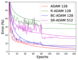
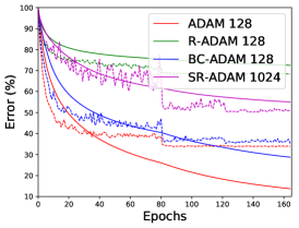
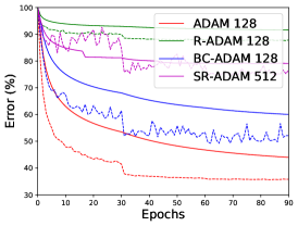
Results The overall results are summarized in Table 1. The binary model trained by BC-ADAM has comparable performance to the full-precision model trained by ADAM. SR-ADAM outperforms R-ADAM, which verifies the effectiveness of Stochastic Rounding. There is a performance gap between SR-ADAM and BC-ADAM across all models and datasets. This is consistent with our theoretical results in Sections 4 and 5, which predict that keeping track of the real-valued weights as in BC-ADAM should produce better minimizers.

Table 1: Top-1 test error after training with full-precision (ADAM), binarized weights (R-ADAM, SR-ADAM, BC-ADAM), and binarized weights with big batch size (Big SR-ADAM).
CIFAR-10 CIFAR-100 ImageNet
VGG-9 VGG-BC ResNet-56 WRN-56-2 ResNet-56 ResNet-18
ADAM   7.97   7.12   8.10   6.62 33.98 36.04
BC-ADAM 10.36   8.21   8.83   7.17 35.34 52.11
Big SR-ADAM 16.95 16.77 19.84 16.04 50.79 77.68
SR-ADAM 23.33 20.56 26.49 21.58 58.06 88.86
R-ADAM 23.99 21.88 33.56 27.90 68.39 91.07

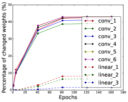
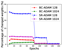
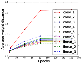
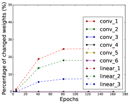
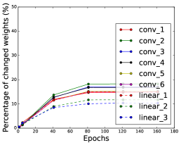
Exploration vs exploitation tradeoffs Section 5 discusses the exploration/exploitation tradeoff of continuous-valued SGD methods and predicts that fully discrete methods like SR are unable to enter a greedy phase. To test this effect, we plot the percentage of changed weights (signs different from the initialization) as a function of the training epochs (Figures 4 and 5). SR-ADAM explores aggressively; it changes more weights in the conv layers than both R-ADAM and BC-ADAM, and keeps changing weights until nearly 40% of the weights differ from their starting values (in a binary model, randomly re-assigning weights would result in 50% change). The BC method never changes more than 20% of the weights (Fig 4(b)), indicating that it stays near a local minimizer and explores less. Interestingly, we see that the weights of the conv layers were not changed at all by R-ADAM; when the tails of the stochastic gradient distribution are light, this method is ineffective.
Refer to caption
(a) R-ADAM
Refer to caption
(b) BC-ADAM
Refer to caption
(c) SR-ADAM
Figure 4: Percentage of weight changes during training of VGG-BC on CIFAR-10.
Refer to caption
(a) BC-ADAM vs SR-ADAM
Refer to caption
(b) Weight changes since beginning
Refer to caption
(c) Weight changes every 5 epochs
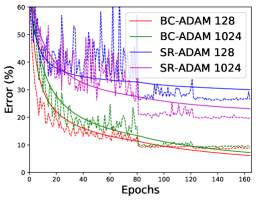
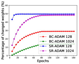
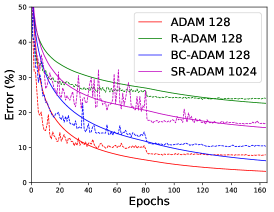
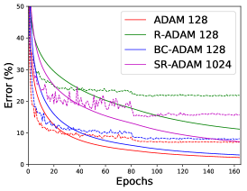
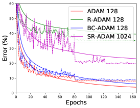
Figure 5: Effect of batch size on SR-ADAM when tested with ResNet-56 on CIFAR-10. (a) Test error vs epoch. Test error is reported with dashed lines, train error with solid lines. (b) Percentage of weight changes since initialization. (c) Percentage of weight changes per every 5 epochs.

6.1 A Way Forward: Big Batch Training

We saw in Section 5 that SR is unable to exploit local minima because, for small learning rates, shrinking the learning rate does not produce additional bias towards moving downhill. This was illustrated in Figure 1. If this is truly the cause of the problem, then our theory predicts that we can improve the performance of SR for low-precision training by increasing the batch size. This shrinks the variance of the gradient distribution in Figure 1 without changing the mean and concentrates more of the gradient distribution towards downhill directions, making the algorithm more greedy.

To verify this, we tried different batch sizes for SR including 128, 256, 512 and 1024, and found that the larger the batch size, the better the performance of SR. Figure 5(a) illustrates the effect of a batch size of 1024 for BC and SR methods. We find that the BC method, like classical SGD, performs best with a small batch size. However, a large batch size is essential for the SR method to perform well. Figure 5(b) shows the percentage of weights changed by SR and BC during training. We see that the large batch methods change the weights less aggressively than the small batch methods, indicating less exploration. Figure 5(c) shows the percentage of weights changed during each 5 epochs of training. It is clear that small-batch SR changes weights much more frequently than using a big batch. This property of big batch training clearly benefits SR; we see in Figure 5(a) and Table 1 that big batch training improved performance over SR-ADAM consistently.

In addition to providing a means of improving fixed-point training, this suggests that recently proposed methods using big batches [28, 29] may be able to exploit lower levels of precision to further accelerate training.

7 Conclusion

The training of quantized neural networks is essential for deploying machine learning models on portable and ubiquitous devices. We provide a theoretical analysis to better understand the BinaryConnect (BC) and Stochastic Rounding (SR) methods for training quantized networks. We proved convergence results for BC and SR methods that predict an accuracy bound that depends on the coarseness of discretization. For general non-convex problems, we proved that SR differs from conventional stochastic methods in that it is unable to exploit greedy local search. Experiments confirm these findings, and show that the mathematical properties of SR are indeed observable (and very important) in practice.

Acknowledgments

T. Goldstein was supported in part by the US National Science Foundation (NSF) under grant CCF-1535902, by the US Office of Naval Research under grant N00014-17-1-2078, and by the Sloan Foundation. C. Studer was supported in part by Xilinx, Inc. and by the US NSF under grants ECCS-1408006, CCF-1535897, and CAREER CCF-1652065. H. Samet was supported in part by the US NSF under grant IIS-13-20791.

References

  • [1] Courbariaux, M., Hubara, I., Soudry, D., El-Yaniv, R., Bengio, Y.: Binarized neural networks: Training deep neural networks with weights and activations constrained to +1 or -1. arXiv preprint arXiv:1602.02830 (2016)
  • [2] Marchesi, M., Orlandi, G., Piazza, F., Uncini, A.: Fast neural networks without multipliers. IEEE Transactions on Neural Networks 4(1) (1993) 53–62
  • [3] Rastegari, M., Ordonez, V., Redmon, J., Farhadi, A.: XNOR-Net: ImageNet Classification Using Binary Convolutional Neural Networks. ECCV (2016)
  • [4] Gupta, S., Agrawal, A., Gopalakrishnan, K., Narayanan, P.: Deep learning with limited numerical precision. In: ICML. (2015)
  • [5] Courbariaux, M., Bengio, Y., David, J.P.: Binaryconnect: Training deep neural networks with binary weights during propagations. In: NIPS. (2015)
  • [6] Lin, D., Talathi, S., Annapureddy, S.: Fixed point quantization of deep convolutional networks. In: ICML. (2016)
  • [7] Hwang, K., Sung, W.: Fixed-point feedforward deep neural network design using weights+ 1, 0, and- 1. In: IEEE Workshop on Signal Processing Systems (SiPS). (2014)
  • [8] Lin, Z., Courbariaux, M., Memisevic, R., Bengio, Y.: Neural networks with few multiplications. ICLR (2016)
  • [9] Li, F., Zhang, B., Liu, B.: Ternary weight networks. arXiv preprint arXiv:1605.04711 (2016)
  • [10] Kim, M., Smaragdis, P.: Bitwise neural networks. In: ICML Workshop on Resource-Efficient Machine Learning. (2015)
  • [11] Hubara, I., Courbariaux, M., Soudry, D., El-Yaniv, R., Bengio, Y.: Quantized neural networks: Training neural networks with low precision weights and activations. arXiv preprint arXiv:1609.07061 (2016)
  • [12] Baldassi, C., Ingrosso, A., Lucibello, C., Saglietti, L., Zecchina, R.: Subdominant dense clusters allow for simple learning and high computational performance in neural networks with discrete synapses. Physical review letters 115(12) (2015) 128101
  • [13] Anwar, S., Hwang, K., Sung, W.: Fixed point optimization of deep convolutional neural networks for object recognition. In: ICASSP, IEEE (2015)
  • [14] Zhu, C., Han, S., Mao, H., Dally, W.J.: Trained ternary quantization. ICLR (2017)
  • [15] Zhou, A., Yao, A., Guo, Y., Xu, L., Chen, Y.: Incremental network quantization: Towards lossless CNNs with low-precision weights. ICLR (2017)
  • [16] Zhou, S., Wu, Y., Ni, Z., Zhou, X., Wen, H., Zou, Y.: Dorefa-net: Training low bitwidth convolutional neural networks with low bitwidth gradients. arXiv preprint arXiv:1606.06160 (2016)
  • [17] Höhfeld, M., Fahlman, S.E.: Probabilistic rounding in neural network learning with limited precision. Neurocomputing 4(6) (1992) 291–299
  • [18] Miyashita, D., Lee, E.H., Murmann, B.: Convolutional neural networks using logarithmic data representation. arXiv preprint arXiv:1603.01025 (2016)
  • [19] Soudry, D., Hubara, I., Meir, R.: Expectation backpropagation: Parameter-free training of multilayer neural networks with continuous or discrete weights. In: NIPS. (2014)
  • [20] Cheng, Z., Soudry, D., Mao, Z., Lan, Z.: Training binary multilayer neural networks for image classification using expectation backpropagation. arXiv preprint arXiv:1503.03562 (2015)
  • [21] Martens, J., Grosse, R.: Optimizing neural networks with kronecker-factored approximate curvature. In: International Conference on Machine Learning. (2015) 2408–2417
  • [22] Lan, G., Nemirovski, A., Shapiro, A.: Validation analysis of mirror descent stochastic approximation method. Mathematical programming 134(2) (2012) 425–458
  • [23] Levin, D.A., Peres, Y., Wilmer, E.L.: Markov chains and mixing times. American Mathematical Soc. (2009)
  • [24] Simonyan, K., Zisserman, A.: Very Deep Convolutional Networks for Large-Scale Image Recognition. In: ICLR. (2015)
  • [25] He, K., Zhang, X., Ren, S., Sun, J.: Deep Residual Learning for Image Recognition. In: CVPR. (2016)
  • [26] Russakovsky, O., Deng, J., Su, H., Krause, J., Satheesh, S., Ma, S., Huang, Z., Karpathy, A., Khosla, A., Bernstein, M., et al.: Imagenet Large Scale Visual Recognition Challenge. IJCV (2015)
  • [27] Kingma, D., Ba, J.: Adam: A method for stochastic optimization. ICLR (2015)
  • [28] De, S., Yadav, A., Jacobs, D., Goldstein, T.: Big batch SGD: Automated inference using adaptive batch sizes. arXiv preprint arXiv:1610.05792 (2016)
  • [29] Goyal, P., Dollár, P., Girshick, R., Noordhuis, P., Wesolowski, L., Kyrola, A., Tulloch, A., Jia, Y., He, K.: Accurate, large minibatch sgd: Training imagenet in 1 hour. arXiv preprint arXiv:1706.02677 (2017)
  • [30] Lax, P.: Linear Algebra and Its Applications. Number v. 10 in Linear algebra and its applications. Wiley (2007)
  • [31] Krizhevsky, A.: Learning multiple layers of features from tiny images. (2009)
  • [32] Zagoruyko, S., Komodakis, N.: Wide residual networks. arXiv preprint arXiv:1605.07146 (2016)
  • [33] Collobert, R., Kavukcuoglu, K., Farabet, C.: Torch7: A matlab-like environment for machine learning. In: BigLearn, NIPS Workshop. (2011)
  • [34] Ioffe, S., Szegedy, C.: Batch Normalization: Accelerating Deep Network Training by Reducing Internal Covariate Shift. (2015)

Training Quantized Nets: A Deeper Understanding

Appendices

Here we present proofs of the lemmas and theorems presented in the main paper, as well as some additional experimental details and results.

Appendix A Proof of Lemma 1

Proof.

We want to bound the quantization error rtsuperscript𝑟𝑡r^{t}. Consider the i𝑖i-th entry in rtsuperscript𝑟𝑡r^{t} denoted by ritsuperscriptsubscript𝑟𝑖𝑡r_{i}^{t}. Similarly, we define witsubscriptsuperscript𝑤𝑡𝑖w^{t}_{i} and f~(wt)i~𝑓subscriptsuperscript𝑤𝑡𝑖\nabla\tilde{f}(w^{t})_{i}. Choose some random number p[0,1]𝑝01p\in[0,1]. The stochastic rounding operation produces a value of rtsuperscript𝑟𝑡r^{t} given by

ritsubscriptsuperscript𝑟𝑡𝑖\displaystyle r^{t}_{i} =Qs(witαtf~(wt)i)wit+αtf~(wt)iabsentsubscript𝑄𝑠superscriptsubscript𝑤𝑖𝑡subscript𝛼𝑡~𝑓subscriptsuperscript𝑤𝑡𝑖superscriptsubscript𝑤𝑖𝑡subscript𝛼𝑡~𝑓subscriptsuperscript𝑤𝑡𝑖\displaystyle=Q_{s}(w_{i}^{t}-\alpha_{t}\nabla\tilde{f}(w^{t})_{i})-w_{i}^{t}+\alpha_{t}\nabla\tilde{f}(w^{t})_{i}
=Δ{αtf~(wt)iΔ+αtf~(wt)iΔ+1,for pαtf~(wt)iΔαtf~(wt)iΔ,αtf~(wt)iΔ+αtf~(wt)iΔ,otherwise,absentΔcasessubscript𝛼𝑡~𝑓subscriptsuperscript𝑤𝑡𝑖Δsubscript𝛼𝑡~𝑓subscriptsuperscript𝑤𝑡𝑖Δ1for 𝑝subscript𝛼𝑡~𝑓subscriptsuperscript𝑤𝑡𝑖Δsubscript𝛼𝑡~𝑓subscriptsuperscript𝑤𝑡𝑖Δsubscript𝛼𝑡~𝑓subscriptsuperscript𝑤𝑡𝑖Δsubscript𝛼𝑡~𝑓subscriptsuperscript𝑤𝑡𝑖Δotherwise,\displaystyle=\Delta\cdot\begin{cases}\displaystyle\frac{\alpha_{t}\nabla\tilde{f}(w^{t})_{i}}{\Delta}+\left\lfloor\frac{-\alpha_{t}\nabla\tilde{f}(w^{t})_{i}}{\Delta}\right\rfloor+1,&\text{for }\,\displaystyle p\leq-\frac{\alpha_{t}\nabla\tilde{f}(w^{t})_{i}}{\Delta}-\left\lfloor\frac{-\alpha_{t}\nabla\tilde{f}(w^{t})_{i}}{\Delta}\right\rfloor,\vspace{2mm}\\ \displaystyle\frac{\alpha_{t}\nabla\tilde{f}(w^{t})_{i}}{\Delta}+\left\lfloor\frac{-\alpha_{t}\nabla\tilde{f}(w^{t})_{i}}{\Delta}\right\rfloor,&\text{otherwise,}\end{cases}
=Δ{q+1,for pq,q,otherwise,absentΔcases𝑞1for 𝑝𝑞𝑞otherwise,\displaystyle=\Delta\cdot\begin{cases}\displaystyle-q+1,&\text{for }\,\displaystyle p\leq q,\vspace{2mm}\\ \displaystyle-q,&\text{otherwise,}\end{cases}

where we write q=αtf~(wt)iΔαtf~(wt)iΔ𝑞subscript𝛼𝑡~𝑓subscriptsuperscript𝑤𝑡𝑖Δsubscript𝛼𝑡~𝑓subscriptsuperscript𝑤𝑡𝑖Δ\displaystyle q=-\frac{\alpha_{t}\nabla\tilde{f}(w^{t})_{i}}{\Delta}-\left\lfloor\frac{-\alpha_{t}\nabla\tilde{f}(w^{t})_{i}}{\Delta}\right\rfloor and q[0,1]𝑞01q\in[0,1].

Now we have

𝔼p[(rit)2]subscript𝔼𝑝delimited-[]superscriptsubscriptsuperscript𝑟𝑡𝑖2\displaystyle\mathbb{E}_{p}\big{[}(r^{t}_{i})^{2}\big{]} Δ2((q+1)2q+(q)2(1q))absentsuperscriptΔ2superscript𝑞12𝑞superscript𝑞21𝑞\displaystyle\leq\Delta^{2}((-q+1)^{2}q+(-q)^{2}(1-q))
=Δ2q(1q)absentsuperscriptΔ2𝑞1𝑞\displaystyle=\Delta^{2}q(1-q)
Δ2min{q,1q}.absentsuperscriptΔ2𝑞1𝑞\displaystyle\leq\Delta^{2}\min\{q,1-q\}.

Because min{q,1q}|αtf~(wt)iΔ|𝑞1𝑞subscript𝛼𝑡~𝑓subscriptsuperscript𝑤𝑡𝑖Δ\displaystyle\min\{q,1-q\}\leq\left|\frac{\alpha_{t}\nabla\tilde{f}(w^{t})_{i}}{\Delta}\right|, it follows that 𝔼p[(rit)2]Δ2|αtf~(wt)iΔ|Δ|αtf~(wt)i|subscript𝔼𝑝delimited-[]superscriptsubscriptsuperscript𝑟𝑡𝑖2superscriptΔ2subscript𝛼𝑡~𝑓subscriptsuperscript𝑤𝑡𝑖ΔΔsubscript𝛼𝑡~𝑓subscriptsuperscript𝑤𝑡𝑖\displaystyle\mathbb{E}_{p}\big{[}(r^{t}_{i})^{2}\big{]}\leq\Delta^{2}\left|\frac{\alpha_{t}\nabla\tilde{f}(w^{t})_{i}}{\Delta}\right|\leq\Delta\left|\alpha_{t}\nabla\tilde{f}(w^{t})_{i}\right|.

Summing over the index i𝑖i yields

𝔼prt22subscript𝔼𝑝subscriptsuperscriptnormsuperscript𝑟𝑡22\displaystyle\mathbb{E}_{p}\big{\|}r^{t}\big{\|}^{2}_{2} Δαtf~(wt)1absentΔsubscript𝛼𝑡subscriptnorm~𝑓superscript𝑤𝑡1\displaystyle\leq\Delta\alpha_{t}\big{\|}\nabla\tilde{f}(w^{t})\big{\|}_{1}
dαtΔf~(wt)2.absent𝑑subscript𝛼𝑡Δsubscriptnorm~𝑓superscript𝑤𝑡2\displaystyle\leq\sqrt{d}\alpha_{t}\Delta\big{\|}\nabla\tilde{f}(w^{t})\big{\|}_{2}. (11)

Now, (𝔼f~(wt)2)2𝔼f~(wt)22G2.superscript𝔼subscriptnorm~𝑓superscript𝑤𝑡22𝔼superscriptsubscriptnorm~𝑓superscript𝑤𝑡22superscript𝐺2\big{(}\mathbb{E}\big{\|}\nabla\tilde{f}(w^{t})\big{\|}_{2}\big{)}^{2}\leq\mathbb{E}\big{\|}\nabla\tilde{f}(w^{t})\big{\|}_{2}^{2}\leq G^{2}. Plugging this into (A) yields

𝔼rt22dΔαtG.𝔼subscriptsuperscriptnormsuperscript𝑟𝑡22𝑑Δsubscript𝛼𝑡𝐺\displaystyle\mathbb{E}\big{\|}r^{t}\big{\|}^{2}_{2}\leq\sqrt{d}\Delta\alpha_{t}G. (12)

Appendix B Proof of Theorem 1

Proof.

From the update rule (6), we get:

wt+1superscript𝑤𝑡1\displaystyle w^{t+1} =Q(wtαtf~(wt))absent𝑄superscript𝑤𝑡subscript𝛼𝑡~𝑓superscript𝑤𝑡\displaystyle=Q\big{(}w^{t}-\alpha_{t}\nabla\tilde{f}(w^{t})\big{)}
=wtαtf~(wt)+rt,absentsuperscript𝑤𝑡subscript𝛼𝑡~𝑓superscript𝑤𝑡superscript𝑟𝑡\displaystyle=w^{t}-\alpha_{t}\nabla\tilde{f}(w^{t})+r^{t},

where rtsuperscript𝑟𝑡r^{t} denotes the quantization used on the t𝑡t-th iteration. Subtracting by the optimal wsuperscript𝑤w^{\star}, taking norm, and taking expectation conditioned on wtsuperscript𝑤𝑡w^{t}, we get:

𝔼wt+1w2𝔼superscriptnormsuperscript𝑤𝑡1superscript𝑤2\displaystyle\mathbb{E}\|w^{t+1}-w^{\star}\|^{2} =wtw22𝔼wtw,αtf~(wt)rt+𝔼αtf~(wt)rt2absentsuperscriptnormsuperscript𝑤𝑡superscript𝑤22𝔼superscript𝑤𝑡superscript𝑤subscript𝛼𝑡~𝑓superscript𝑤𝑡superscript𝑟𝑡𝔼superscriptnormsubscript𝛼𝑡~𝑓superscript𝑤𝑡superscript𝑟𝑡2\displaystyle=\|w^{t}-w^{\star}\|^{2}-2\mathbb{E}\langle w^{t}-w^{\star},\alpha_{t}\nabla\tilde{f}(w^{t})-r^{t}\rangle+\mathbb{E}\|\alpha_{t}\nabla\tilde{f}(w^{t})-r^{t}\|^{2}
=wtw22αtwtw,F(wt)+αt2𝔼f~(wt)2+𝔼rt2absentsuperscriptnormsuperscript𝑤𝑡superscript𝑤22subscript𝛼𝑡superscript𝑤𝑡superscript𝑤𝐹superscript𝑤𝑡superscriptsubscript𝛼𝑡2𝔼superscriptnorm~𝑓superscript𝑤𝑡2𝔼superscriptnormsuperscript𝑟𝑡2\displaystyle=\|w^{t}-w^{\star}\|^{2}-2\alpha_{t}\langle w^{t}-w^{\star},\nabla F(w^{t})\rangle+\alpha_{t}^{2}\mathbb{E}\|\nabla\tilde{f}(w^{t})\|^{2}+\mathbb{E}\|r^{t}\|^{2}
wtw22αtwtw,F(wt)+αt2G2+dΔαtG,absentsuperscriptnormsuperscript𝑤𝑡superscript𝑤22subscript𝛼𝑡superscript𝑤𝑡superscript𝑤𝐹superscript𝑤𝑡superscriptsubscript𝛼𝑡2superscript𝐺2𝑑Δsubscript𝛼𝑡𝐺\displaystyle\leq\|w^{t}-w^{\star}\|^{2}-2\alpha_{t}\langle w^{t}-w^{\star},\nabla F(w^{t})\rangle+\alpha_{t}^{2}G^{2}+\sqrt{d}\Delta\alpha_{t}G,

where we use the bounded variance assumption, 𝔼[rt]=0𝔼delimited-[]superscript𝑟𝑡0\mathbb{E}[r^{t}]=0, and Lemma 1. Using the assumption that F𝐹F is μ𝜇\mu-strongly convex, we can simplify this to:

𝔼wt+1w2𝔼superscriptnormsuperscript𝑤𝑡1superscript𝑤2\displaystyle\mathbb{E}\|w^{t+1}-w^{\star}\|^{2} (1αtμ)wtw22αt(F(wt)F(w))+αt2G2+dΔαtG.absent1subscript𝛼𝑡𝜇superscriptnormsuperscript𝑤𝑡superscript𝑤22subscript𝛼𝑡𝐹superscript𝑤𝑡𝐹superscript𝑤superscriptsubscript𝛼𝑡2superscript𝐺2𝑑Δsubscript𝛼𝑡𝐺\displaystyle\leq(1-\alpha_{t}\mu)\|w^{t}-w^{\star}\|^{2}-2\alpha_{t}(F(w^{t})-F(w^{\star}))+\alpha_{t}^{2}G^{2}+\sqrt{d}\Delta\alpha_{t}G.

Re-arranging the terms, and taking expectation we get:

2αt𝔼(F(wt)F(w))2subscript𝛼𝑡𝔼𝐹superscript𝑤𝑡𝐹superscript𝑤\displaystyle 2\alpha_{t}\mathbb{E}(F(w^{t})-F(w^{\star})) (1αtμ)𝔼wtw2𝔼wt+1w2+αt2G2+dΔαtG.absent1subscript𝛼𝑡𝜇𝔼superscriptnormsuperscript𝑤𝑡superscript𝑤2𝔼superscriptnormsuperscript𝑤𝑡1superscript𝑤2superscriptsubscript𝛼𝑡2superscript𝐺2𝑑Δsubscript𝛼𝑡𝐺\displaystyle\leq(1-\alpha_{t}\mu)\mathbb{E}\|w^{t}-w^{\star}\|^{2}-\mathbb{E}\|w^{t+1}-w^{\star}\|^{2}+\alpha_{t}^{2}G^{2}+\sqrt{d}\Delta\alpha_{t}G.
𝔼(F(wt)F(w))𝔼𝐹superscript𝑤𝑡𝐹superscript𝑤\displaystyle\Rightarrow\quad\mathbb{E}(F(w^{t})-F(w^{\star})) (12αtμ2)𝔼wtw212αt𝔼wt+1w2+αt2G2+dΔG2.absent12subscript𝛼𝑡𝜇2𝔼superscriptnormsuperscript𝑤𝑡superscript𝑤212subscript𝛼𝑡𝔼superscriptnormsuperscript𝑤𝑡1superscript𝑤2subscript𝛼𝑡2superscript𝐺2𝑑Δ𝐺2\displaystyle\leq\left(\frac{1}{2\alpha_{t}}-\frac{\mu}{2}\right)\mathbb{E}\|w^{t}-w^{\star}\|^{2}-\frac{1}{2\alpha_{t}}\mathbb{E}\|w^{t+1}-w^{\star}\|^{2}+\frac{\alpha_{t}}{2}G^{2}+\frac{\sqrt{d}\Delta G}{2}.

Assume that the stepsize decreases with the rate αt=1/μ(t+1)subscript𝛼𝑡1𝜇𝑡1\alpha_{t}=1/\mu(t+1). Then we have:

𝔼(F(wt)F(w))μt2𝔼wtw2μ(t+1)2𝔼wt+1w2+12μ(t+1)G2+dΔG2.𝔼𝐹superscript𝑤𝑡𝐹superscript𝑤𝜇𝑡2𝔼superscriptnormsuperscript𝑤𝑡superscript𝑤2𝜇𝑡12𝔼superscriptnormsuperscript𝑤𝑡1superscript𝑤212𝜇𝑡1superscript𝐺2𝑑Δ𝐺2\displaystyle\mathbb{E}(F(w^{t})-F(w^{\star}))\leq\frac{\mu t}{2}\mathbb{E}\|w^{t}-w^{\star}\|^{2}-\frac{\mu(t+1)}{2}\mathbb{E}\|w^{t+1}-w^{\star}\|^{2}+\frac{1}{2\mu(t+1)}G^{2}+\frac{\sqrt{d}\Delta G}{2}.

Averaging over t=0𝑡0t=0 to T𝑇T, we get a telescoping sum on the right hand side, which yields:

1Tt=0T𝔼(F(wt)F(w))1𝑇superscriptsubscript𝑡0𝑇𝔼𝐹superscript𝑤𝑡𝐹superscript𝑤\displaystyle\frac{1}{T}\sum_{t=0}^{T}\mathbb{E}(F(w^{t})-F(w^{\star})) G22μTt=0T1t+1+dΔG2μ(T+1)2𝔼wT+1w2absentsuperscript𝐺22𝜇𝑇superscriptsubscript𝑡0𝑇1𝑡1𝑑Δ𝐺2𝜇𝑇12𝔼superscriptnormsuperscript𝑤𝑇1superscript𝑤2\displaystyle\leq\frac{G^{2}}{2\mu T}\sum_{t=0}^{T}\frac{1}{t+1}+\frac{\sqrt{d}\Delta G}{2}-\frac{\mu(T+1)}{2}\mathbb{E}\|w^{T+1}-w^{\star}\|^{2}
(1+log(T+1))G22μT+dΔG2.absent1𝑇1superscript𝐺22𝜇𝑇𝑑Δ𝐺2\displaystyle\leq\frac{(1+\log(T+1))G^{2}}{2\mu T}+\frac{\sqrt{d}\Delta G}{2}.

Using Jensen’s inequality, we have:

𝔼(F(w¯T)F(w))1Tt=0T𝔼(F(wt)F(w)),𝔼𝐹superscript¯𝑤𝑇𝐹superscript𝑤1𝑇superscriptsubscript𝑡0𝑇𝔼𝐹superscript𝑤𝑡𝐹superscript𝑤\displaystyle\mathbb{E}(F(\bar{w}^{T})-F(w^{\star}))\leq\frac{1}{T}\sum_{t=0}^{T}\mathbb{E}(F(w^{t})-F(w^{\star})),

where w¯T=1Tt=0Twtsuperscript¯𝑤𝑇1𝑇superscriptsubscript𝑡0𝑇superscript𝑤𝑡\bar{w}^{T}=\frac{1}{T}\sum_{t=0}^{T}w^{t}, the average of the iterates.

Thus the final convergence theorem is given by:

𝔼[F(w¯T)F(w)](1+log(T+1))G22μT+dΔG2.𝔼delimited-[]𝐹superscript¯𝑤𝑇𝐹superscript𝑤1𝑇1superscript𝐺22𝜇𝑇𝑑Δ𝐺2\displaystyle\mathbb{E}[F(\bar{w}^{T})-F(w^{\star})]\leq\frac{(1+\log(T+1))G^{2}}{2\mu T}+\frac{\sqrt{d}\Delta G}{2}.

Appendix C Proof of Theorem 2

Proof.

From the update rule (6), we have,

wt+1=Q(wtαtf~(wt))=wtαtf~(wt)+rt,superscript𝑤𝑡1𝑄superscript𝑤𝑡subscript𝛼𝑡~𝑓superscript𝑤𝑡superscript𝑤𝑡subscript𝛼𝑡~𝑓superscript𝑤𝑡superscript𝑟𝑡\displaystyle w^{t+1}=Q\big{(}w^{t}-\alpha_{t}\nabla\tilde{f}(w^{t})\big{)}=w^{t}-\alpha_{t}\nabla\tilde{f}(w^{t})+r^{t},

where rtsuperscript𝑟𝑡r^{t} denotes the quantization error on the t𝑡t-th iteration. Hence we have

wt+1w2superscriptnormsuperscript𝑤𝑡1superscript𝑤2\displaystyle\|w^{t+1}-w^{\star}\|^{2} =wtαtf~(wt)+rtw2absentsuperscriptnormsuperscript𝑤𝑡subscript𝛼𝑡~𝑓superscript𝑤𝑡superscript𝑟𝑡superscript𝑤2\displaystyle=\|w^{t}-\alpha_{t}\nabla\tilde{f}(w^{t})+r^{t}-w^{\star}\|^{2}
=wtw22wtw,αtf~(wt)rt+αtf~(wt)rt2.absentsuperscriptnormsuperscript𝑤𝑡superscript𝑤22superscript𝑤𝑡superscript𝑤subscript𝛼𝑡~𝑓superscript𝑤𝑡superscript𝑟𝑡superscriptnormsubscript𝛼𝑡~𝑓superscript𝑤𝑡superscript𝑟𝑡2\displaystyle=\|w^{t}-w^{\star}\|^{2}-2\langle w^{t}-w^{\star},\alpha_{t}\nabla\tilde{f}(w^{t})-r^{t}\rangle+\|\alpha_{t}\nabla\tilde{f}(w^{t})-r^{t}\|^{2}.

Taking expectation, and using 𝔼[f~(wt)]=F(wt)𝔼delimited-[]~𝑓superscript𝑤𝑡𝐹superscript𝑤𝑡\mathbb{E}[\tilde{f}(w^{t})]=\nabla F(w^{t}) and 𝔼[rt]=0𝔼delimited-[]superscript𝑟𝑡0\mathbb{E}[r^{t}]=0, we have

𝔼wt+1w2𝔼superscriptnormsuperscript𝑤𝑡1superscript𝑤2\displaystyle\mathbb{E}\|w^{t+1}-w^{\star}\|^{2} =𝔼wtw22αt𝔼wtw,F(wt)+𝔼αtf~(wt)rt2absent𝔼superscriptnormsuperscript𝑤𝑡superscript𝑤22subscript𝛼𝑡𝔼superscript𝑤𝑡superscript𝑤𝐹superscript𝑤𝑡𝔼superscriptnormsubscript𝛼𝑡~𝑓superscript𝑤𝑡superscript𝑟𝑡2\displaystyle=\mathbb{E}\|w^{t}-w^{\star}\|^{2}-2\alpha_{t}\mathbb{E}\langle w^{t}-w^{\star},\nabla F(w^{t})\rangle+\mathbb{E}\|\alpha_{t}\nabla\tilde{f}(w^{t})-r^{t}\|^{2}
=𝔼wtw22αt𝔼wtw,F(wt)+αt2𝔼f~(wt)2+𝔼rt2.absent𝔼superscriptnormsuperscript𝑤𝑡superscript𝑤22subscript𝛼𝑡𝔼superscript𝑤𝑡superscript𝑤𝐹superscript𝑤𝑡superscriptsubscript𝛼𝑡2𝔼superscriptnorm~𝑓superscript𝑤𝑡2𝔼superscriptnormsuperscript𝑟𝑡2\displaystyle=\mathbb{E}\|w^{t}-w^{\star}\|^{2}-2\alpha_{t}\mathbb{E}\langle w^{t}-w^{\star},\nabla F(w^{t})\rangle+\alpha_{t}^{2}\mathbb{E}\|\nabla\tilde{f}(w^{t})\|^{2}+\mathbb{E}\|r^{t}\|^{2}.

Using the bounded variance assumption 𝔼f~(wt)2G2𝔼superscriptnorm~𝑓superscript𝑤𝑡2superscript𝐺2\mathbb{E}\|\nabla\tilde{f}(w^{t})\|^{2}\leq G^{2} and bounded quantization error in Lemma 1, we have

𝔼wt+1w2𝔼wtw22αt𝔼wtw,F(wt)+αt2G2+dΔαtG.𝔼superscriptnormsuperscript𝑤𝑡1superscript𝑤2𝔼superscriptnormsuperscript𝑤𝑡superscript𝑤22subscript𝛼𝑡𝔼superscript𝑤𝑡superscript𝑤𝐹superscript𝑤𝑡superscriptsubscript𝛼𝑡2superscript𝐺2𝑑Δsubscript𝛼𝑡𝐺\displaystyle\mathbb{E}\|w^{t+1}-w^{\star}\|^{2}\leq\mathbb{E}\|w^{t}-w^{\star}\|^{2}-2\alpha_{t}\mathbb{E}\langle w^{t}-w^{\star},\nabla F(w^{t})\rangle+\alpha_{t}^{2}G^{2}+\sqrt{d}\Delta\alpha_{t}G. (13)

F(x)𝐹𝑥F(x) is convex and hence F(x),xtxF(xt)F(x)𝐹𝑥subscript𝑥𝑡superscript𝑥𝐹subscript𝑥𝑡𝐹superscript𝑥\langle\nabla F(x),x_{t}-x^{\star}\rangle\geq F(x_{t})-F(x^{*}), which can be used in (13) to get

𝔼wt+1w2𝔼wtw22αt𝔼[F(wt)F(w)]+αt2G2+dΔαtG.𝔼superscriptnormsuperscript𝑤𝑡1superscript𝑤2𝔼superscriptnormsuperscript𝑤𝑡superscript𝑤22subscript𝛼𝑡𝔼delimited-[]𝐹superscript𝑤𝑡𝐹superscript𝑤superscriptsubscript𝛼𝑡2superscript𝐺2𝑑Δsubscript𝛼𝑡𝐺\displaystyle\mathbb{E}\|w^{t+1}-w^{\star}\|^{2}\leq\mathbb{E}\|w^{t}-w^{\star}\|^{2}-2\alpha_{t}\mathbb{E}[F(w^{t})-F(w^{\star})]+\alpha_{t}^{2}G^{2}+\sqrt{d}\Delta\alpha_{t}G.

Re-arranging the terms, we have,

𝔼[F(wt)F(w)]12αt(𝔼wtw2𝔼wt+1w2)+αt2G2+12dΔG.𝔼delimited-[]𝐹superscript𝑤𝑡𝐹superscript𝑤12subscript𝛼𝑡𝔼superscriptnormsuperscript𝑤𝑡superscript𝑤2𝔼superscriptnormsuperscript𝑤𝑡1superscript𝑤2subscript𝛼𝑡2superscript𝐺212𝑑Δ𝐺\displaystyle\mathbb{E}[F(w^{t})-F(w^{\star})]\leq\frac{1}{2\alpha_{t}}\left(\mathbb{E}\|w^{t}-w^{\star}\|^{2}-\mathbb{E}\|w^{t+1}-w^{\star}\|^{2}\right)+\frac{\alpha_{t}}{2}G^{2}+\frac{1}{2}\sqrt{d}\Delta G.

Accumulate from t=1𝑡1t=1 to T𝑇T to get

t=1T𝔼[F(wt)F(w)]superscriptsubscript𝑡1𝑇𝔼delimited-[]𝐹superscript𝑤𝑡𝐹superscript𝑤absent\displaystyle\sum_{t=1}^{T}\mathbb{E}[F(w^{t})-F(w^{\star})]\leq 12α1𝔼w1w2+t=1T(12αt12αt1)𝔼wtw212subscript𝛼1𝔼superscriptnormsubscript𝑤1superscript𝑤2superscriptsubscript𝑡1𝑇12subscript𝛼𝑡12subscript𝛼𝑡1𝔼superscriptnormsuperscript𝑤𝑡superscript𝑤2\displaystyle\frac{1}{2\alpha_{1}}\mathbb{E}\|w_{1}-w^{\star}\|^{2}+\sum_{t=1}^{T}\left(\frac{1}{2\alpha_{t}}-\frac{1}{2\alpha_{t-1}}\right)\mathbb{E}\|w^{t}-w^{\star}\|^{2}
+t=1Tαt2G2+T2dΔG.superscriptsubscript𝑡1𝑇subscript𝛼𝑡2superscript𝐺2𝑇2𝑑Δ𝐺\displaystyle+\sum_{t=1}^{T}\frac{\alpha_{t}}{2}G^{2}+\frac{T}{2}\sqrt{d}\Delta G.

Applying 𝔼wtw2D2𝔼superscriptnormsuperscript𝑤𝑡superscript𝑤2superscript𝐷2\mathbb{E}\|w^{t}-w^{\star}\|^{2}\leq D^{2} and t=1TαtcT+1superscriptsubscript𝑡1𝑇subscript𝛼𝑡𝑐𝑇1\sum_{t=1}^{T}\alpha_{t}\leq c\sqrt{T+1}, we have

t=1T𝔼[F(wt)F(w)]T2cD2+cT+12G2+T2dΔG.superscriptsubscript𝑡1𝑇𝔼delimited-[]𝐹superscript𝑤𝑡𝐹superscript𝑤𝑇2𝑐superscript𝐷2𝑐𝑇12superscript𝐺2𝑇2𝑑Δ𝐺\displaystyle\sum_{t=1}^{T}\mathbb{E}[F(w^{t})-F(w^{\star})]\leq\frac{\sqrt{T}}{2c}D^{2}+\frac{c\sqrt{T+1}}{2}G^{2}+\frac{T}{2}\sqrt{d}\Delta G. (14)

Since F(w)𝐹𝑤F(w) is convex, we can set w¯T=1Tt=1Twtsuperscript¯𝑤𝑇1𝑇superscriptsubscript𝑡1𝑇superscript𝑤𝑡\bar{w}^{T}=\frac{1}{T}\sum_{t=1}^{T}w^{t}, and use Jensen’s inequality to arrive at

𝔼[F(w¯T)F(w)]1Tt=1T𝔼[F(wt)F(w)].𝔼delimited-[]𝐹superscript¯𝑤𝑇𝐹superscript𝑤1𝑇superscriptsubscript𝑡1𝑇𝔼delimited-[]𝐹superscript𝑤𝑡𝐹superscript𝑤\mathbb{E}[F(\bar{w}^{T})-F(w^{\star})]\leq\frac{1}{T}\sum_{t=1}^{T}\mathbb{E}[F(w^{t})-F(w^{\star})]. (15)

Combine (14) and (15) to achieve

𝔼[F(w¯T)F(w)]12cTD2+T+12TcG2+dΔG2.𝔼delimited-[]𝐹superscript¯𝑤𝑇𝐹superscript𝑤12𝑐𝑇superscript𝐷2𝑇12𝑇𝑐superscript𝐺2𝑑Δ𝐺2\displaystyle\mathbb{E}[F(\bar{w}^{T})-F(w^{\star})]\leq\frac{1}{2c\sqrt{T}}D^{2}+\frac{\sqrt{T+1}}{2T}cG^{2}+\frac{\sqrt{d}\Delta G}{2}.

Appendix D Proof of Theorem 3

Proof.

From the update rule (7), we have,

wt+1=wtαtf~(Q(wt))=wtαtf~(wt+rt).superscript𝑤𝑡1superscript𝑤𝑡subscript𝛼𝑡~𝑓𝑄superscript𝑤𝑡superscript𝑤𝑡subscript𝛼𝑡~𝑓superscript𝑤𝑡superscript𝑟𝑡\displaystyle w^{t+1}=w^{t}-\alpha_{t}\nabla\tilde{f}\big{(}Q(w^{t})\big{)}=w^{t}-\alpha_{t}\nabla\tilde{f}\big{(}w^{t}+r^{t}\big{)}.

Taking expectation conditioned on wtsuperscript𝑤𝑡w^{t} and rtsuperscript𝑟𝑡r^{t}, we have

𝔼wt+1w2𝔼superscriptnormsuperscript𝑤𝑡1superscript𝑤2\displaystyle\mathbb{E}\|w^{t+1}-w^{\star}\|^{2}
=𝔼wtαtf~(wt+rt)w2absent𝔼superscriptnormsuperscript𝑤𝑡subscript𝛼𝑡~𝑓superscript𝑤𝑡superscript𝑟𝑡superscript𝑤2\displaystyle=\mathbb{E}\|w^{t}-\alpha_{t}\nabla\tilde{f}\big{(}w^{t}+r^{t}\big{)}-w^{\star}\|^{2}
=𝔼wtαtf~(wt)+αtf~(wt)αtf~(wt+rt)w2absent𝔼superscriptnormsuperscript𝑤𝑡subscript𝛼𝑡~𝑓superscript𝑤𝑡subscript𝛼𝑡~𝑓superscript𝑤𝑡subscript𝛼𝑡~𝑓superscript𝑤𝑡superscript𝑟𝑡superscript𝑤2\displaystyle=\mathbb{E}\|w^{t}-\alpha_{t}\nabla\tilde{f}\big{(}w^{t})+\alpha_{t}\nabla\tilde{f}\big{(}w^{t}\big{)}-\alpha_{t}\nabla\tilde{f}\big{(}w^{t}+r^{t}\big{)}-w^{\star}\|^{2}
=wtw22αt𝔼wtw,f~(wt)+2αt𝔼wtw,f~(wt)f~(wt+rt)+𝔼αtf~(wt+rt)2absentsuperscriptnormsuperscript𝑤𝑡superscript𝑤22subscript𝛼𝑡𝔼superscript𝑤𝑡superscript𝑤~𝑓superscript𝑤𝑡2subscript𝛼𝑡𝔼superscript𝑤𝑡superscript𝑤~𝑓superscript𝑤𝑡~𝑓superscript𝑤𝑡superscript𝑟𝑡𝔼superscriptnormsubscript𝛼𝑡~𝑓superscript𝑤𝑡superscript𝑟𝑡2\displaystyle=\|w^{t}-w^{\star}\|^{2}-2\alpha_{t}\mathbb{E}\langle w^{t}-w^{\star},\nabla\tilde{f}\big{(}w^{t}\big{)}\rangle+2\alpha_{t}\mathbb{E}\langle w^{t}-w^{\star},\nabla\tilde{f}\big{(}w^{t}\big{)}-\nabla\tilde{f}\big{(}w^{t}+r^{t}\big{)}\rangle+\mathbb{E}\|\alpha_{t}\nabla\tilde{f}\big{(}w^{t}+r^{t}\big{)}\|^{2}
=wtw22αtwtw,F(wt)+2αtwtw,F(wt)F(wt+rt)+αt2𝔼f~(wt+rt)2absentsuperscriptnormsuperscript𝑤𝑡superscript𝑤22subscript𝛼𝑡superscript𝑤𝑡superscript𝑤𝐹superscript𝑤𝑡2subscript𝛼𝑡superscript𝑤𝑡superscript𝑤𝐹superscript𝑤𝑡𝐹superscript𝑤𝑡superscript𝑟𝑡superscriptsubscript𝛼𝑡2𝔼superscriptnorm~𝑓superscript𝑤𝑡superscript𝑟𝑡2\displaystyle=\|w^{t}-w^{\star}\|^{2}-2\alpha_{t}\langle w^{t}-w^{\star},\nabla F\big{(}w^{t}\big{)}\rangle+2\alpha_{t}\langle w^{t}-w^{\star},\nabla F\big{(}w^{t}\big{)}-\nabla F\big{(}w^{t}+r^{t}\big{)}\rangle+\alpha_{t}^{2}\mathbb{E}\|\nabla\tilde{f}\big{(}w^{t}+r^{t}\big{)}\|^{2}
wtw22αtwtw,F(wt)+2αtwtwF(wt)F(wt+rt)+αt2G2absentsuperscriptnormsuperscript𝑤𝑡superscript𝑤22subscript𝛼𝑡superscript𝑤𝑡superscript𝑤𝐹superscript𝑤𝑡2subscript𝛼𝑡normsuperscript𝑤𝑡superscript𝑤norm𝐹superscript𝑤𝑡𝐹superscript𝑤𝑡superscript𝑟𝑡superscriptsubscript𝛼𝑡2superscript𝐺2\displaystyle\leq\|w^{t}-w^{\star}\|^{2}-2\alpha_{t}\langle w^{t}-w^{\star},\nabla F\big{(}w^{t}\big{)}\rangle+2\alpha_{t}\|w^{t}-w^{\star}\|\|\nabla F\big{(}w^{t}\big{)}-\nabla F\big{(}w^{t}+r^{t}\big{)}\|+\alpha_{t}^{2}G^{2}
wtw22αtwtw,F(wt)+2αtLrtwtw+αt2G2.absentsuperscriptnormsuperscript𝑤𝑡superscript𝑤22subscript𝛼𝑡superscript𝑤𝑡superscript𝑤𝐹superscript𝑤𝑡2subscript𝛼𝑡𝐿normsuperscript𝑟𝑡normsuperscript𝑤𝑡superscript𝑤superscriptsubscript𝛼𝑡2superscript𝐺2\displaystyle\leq\|w^{t}-w^{\star}\|^{2}-2\alpha_{t}\langle w^{t}-w^{\star},\nabla F\big{(}w^{t}\big{)}\rangle+2\alpha_{t}L\|r^{t}\|\|w^{t}-w^{\star}\|+\alpha_{t}^{2}G^{2}.

Using rtdΔnormsuperscript𝑟𝑡𝑑Δ\|r^{t}\|\leq\sqrt{d}\Delta and the bounded domain assumption, we get

𝔼wt+1w2𝔼superscriptnormsuperscript𝑤𝑡1superscript𝑤2\displaystyle\mathbb{E}\|w^{t+1}-w^{\star}\|^{2} wtw22αtwtw,F(wt)+2αtLdΔwtw+αt2G2absentsuperscriptnormsuperscript𝑤𝑡superscript𝑤22subscript𝛼𝑡superscript𝑤𝑡superscript𝑤𝐹superscript𝑤𝑡2subscript𝛼𝑡𝐿𝑑Δnormsuperscript𝑤𝑡superscript𝑤superscriptsubscript𝛼𝑡2superscript𝐺2\displaystyle\leq\|w^{t}-w^{\star}\|^{2}-2\alpha_{t}\langle w^{t}-w^{\star},\nabla F\big{(}w^{t}\big{)}\rangle+2\alpha_{t}L\sqrt{d}\Delta\|w^{t}-w^{\star}\|+\alpha_{t}^{2}G^{2}
wtw22αtwtw,F(wt)+2αtLdΔD+αt2G2.absentsuperscriptnormsuperscript𝑤𝑡superscript𝑤22subscript𝛼𝑡superscript𝑤𝑡superscript𝑤𝐹superscript𝑤𝑡2subscript𝛼𝑡𝐿𝑑Δ𝐷superscriptsubscript𝛼𝑡2superscript𝐺2\displaystyle\leq\|w^{t}-w^{\star}\|^{2}-2\alpha_{t}\langle w^{t}-w^{\star},\nabla F\big{(}w^{t}\big{)}\rangle+2\alpha_{t}L\sqrt{d}\Delta D+\alpha_{t}^{2}G^{2}.

Taking expectation, and following the same steps as in Theorem 2, we get the convergence result:

𝔼[F(w¯T)F(w)]12cTD2+T+12TcG2+dΔLD.𝔼delimited-[]𝐹superscript¯𝑤𝑇𝐹superscript𝑤12𝑐𝑇superscript𝐷2𝑇12𝑇𝑐superscript𝐺2𝑑Δ𝐿𝐷\displaystyle\mathbb{E}[F(\bar{w}^{T})-F(w^{\star})]\leq\frac{1}{2c\sqrt{T}}D^{2}+\frac{\sqrt{T+1}}{2T}cG^{2}+\sqrt{d}\Delta LD.

Appendix E Proof of Theorem 4

Proof.

From the update rule (7), we get

wt+1superscript𝑤𝑡1\displaystyle w^{t+1} =wtαtf~(Q(wt))absentsuperscript𝑤𝑡subscript𝛼𝑡~𝑓𝑄superscript𝑤𝑡\displaystyle=w^{t}-\alpha_{t}\nabla\tilde{f}\big{(}Q(w^{t})\big{)}
=wtαtf~(wt+rt)absentsuperscript𝑤𝑡subscript𝛼𝑡~𝑓superscript𝑤𝑡superscript𝑟𝑡\displaystyle=w^{t}-\alpha_{t}\nabla\tilde{f}\big{(}w^{t}+r^{t}\big{)}
=wtαt[f~(wt)+2f~(wt)rt+r^t]absentsuperscript𝑤𝑡subscript𝛼𝑡delimited-[]~𝑓superscript𝑤𝑡superscript2~𝑓superscript𝑤𝑡superscript𝑟𝑡superscript^𝑟𝑡\displaystyle=w^{t}-\alpha_{t}[\nabla\tilde{f}\big{(}w^{t}\big{)}+\nabla^{2}\tilde{f}\big{(}w^{t}\big{)}r^{t}+\hat{r}^{t}]

where r^tL22rt2normsuperscript^𝑟𝑡subscript𝐿22superscriptnormsuperscript𝑟𝑡2\|\hat{r}^{t}\|\leq\frac{L_{2}}{2}\|r^{t}\|^{2} from our assumption on the Hessian. Note that in general rtsuperscript𝑟𝑡r^{t} has mean zero while r^tsuperscript^𝑟𝑡\hat{r}^{t} does not. Using the same steps as in the Theorem 1, we get

𝔼wt+1w2𝔼superscriptnormsuperscript𝑤𝑡1superscript𝑤2\displaystyle\mathbb{E}\|w^{t+1}-w^{\star}\|^{2} =wtw22αt𝔼wtw,f~(wt+rt)+αt2𝔼f~(wt+rt)2.absentsuperscriptnormsuperscript𝑤𝑡superscript𝑤22subscript𝛼𝑡𝔼superscript𝑤𝑡superscript𝑤~𝑓superscript𝑤𝑡superscript𝑟𝑡superscriptsubscript𝛼𝑡2𝔼superscriptnorm~𝑓superscript𝑤𝑡superscript𝑟𝑡2\displaystyle=\|w^{t}-w^{\star}\|^{2}-2\alpha_{t}\mathbb{E}\langle w^{t}-w^{\star},\nabla\tilde{f}(w^{t}+r^{t})\rangle+\alpha_{t}^{2}\mathbb{E}\|\nabla\tilde{f}(w^{t}+r^{t})\|^{2}.
wtw22αt𝔼wtw,F(wt)+r^t+αt2G2absentsuperscriptnormsuperscript𝑤𝑡superscript𝑤22subscript𝛼𝑡𝔼superscript𝑤𝑡superscript𝑤𝐹superscript𝑤𝑡superscript^𝑟𝑡superscriptsubscript𝛼𝑡2superscript𝐺2\displaystyle\leq\|w^{t}-w^{\star}\|^{2}-2\alpha_{t}\mathbb{E}\langle w^{t}-w^{\star},\nabla F(w^{t})+\hat{r}^{t}\rangle+\alpha_{t}^{2}G^{2}
=wtw22αt𝔼wtw,F(wt)+αt2G22αt𝔼wtw,r^tabsentsuperscriptnormsuperscript𝑤𝑡superscript𝑤22subscript𝛼𝑡𝔼superscript𝑤𝑡superscript𝑤𝐹superscript𝑤𝑡superscriptsubscript𝛼𝑡2superscript𝐺22subscript𝛼𝑡𝔼superscript𝑤𝑡superscript𝑤superscript^𝑟𝑡\displaystyle=\|w^{t}-w^{\star}\|^{2}-2\alpha_{t}\mathbb{E}\langle w^{t}-w^{\star},\nabla F(w^{t})\rangle+\alpha_{t}^{2}G^{2}-2\alpha_{t}\mathbb{E}\langle w^{t}-w^{\star},\hat{r}^{t}\rangle

Assuming the domain has finite diameter D𝐷D, and observing that the quantization error for BC-SGD can always be upper-bounded as rtdΔnormsuperscript𝑟𝑡𝑑Δ\|r^{t}\|\leq\sqrt{d}\Delta, we get:

2αt𝔼wtw,r^t2αtD𝔼r^t2αtDL22rtαtDL2dΔ.2subscript𝛼𝑡𝔼superscript𝑤𝑡superscript𝑤superscript^𝑟𝑡2subscript𝛼𝑡𝐷𝔼normsuperscript^𝑟𝑡2subscript𝛼𝑡𝐷subscript𝐿22normsuperscript𝑟𝑡subscript𝛼𝑡𝐷subscript𝐿2𝑑Δ-2\alpha_{t}\mathbb{E}\langle w^{t}-w^{\star},\hat{r}^{t}\rangle\leq 2\alpha_{t}D\mathbb{E}\|\hat{r}^{t}\|\leq 2\alpha_{t}D\frac{L_{2}}{2}\|r^{t}\|\leq\alpha_{t}DL_{2}\sqrt{d}\Delta.

Following the same steps as in Theorem 1, we get

𝔼[F(w¯T)F(w)](1+log(T+1))G22μT+DL2dΔ2.𝔼delimited-[]𝐹superscript¯𝑤𝑇𝐹superscript𝑤1𝑇1superscript𝐺22𝜇𝑇𝐷subscript𝐿2𝑑Δ2\displaystyle\mathbb{E}[F(\bar{w}^{T})-F(w^{\star})]\leq\frac{(1+\log(T+1))G^{2}}{2\mu T}+\frac{DL_{2}\sqrt{d}\Delta}{2}.

Appendix F Proof of Theorem 5

Proof.

Let the matrix Uαsubscript𝑈𝛼U_{\alpha} be a partial transition matrix defined by Uα(x,x)=0,subscript𝑈𝛼𝑥𝑥0U_{\alpha}(x,x)=0, and Uα(x,y)=Tα(x,y)subscript𝑈𝛼𝑥𝑦subscript𝑇𝛼𝑥𝑦U_{\alpha}(x,y)=T_{\alpha}(x,y) for xy.𝑥𝑦x\neq y. From Uα,subscript𝑈𝛼U_{\alpha}, we can get back the full transition matrix Tαsubscript𝑇𝛼T_{\alpha} using the formula

Tα=Idiag(𝟏TUα)+Uα.subscript𝑇𝛼𝐼diagsuperscript1𝑇subscript𝑈𝛼subscript𝑈𝛼T_{\alpha}=I-\operatorname*{diag}(\mathbf{1}^{T}U_{\alpha})+U_{\alpha}.

Note that this formula is essentially “filling in” the diagonal entries of Tαsubscript𝑇𝛼T_{\alpha} so that every column sums to 1, thus making Tαsubscript𝑇𝛼T_{\alpha} a valid stochastic matrix.

Let’s bound the entries in Uα.subscript𝑈𝛼U_{\alpha}. Suppose that we begin an iteration of the stochastic rounding algorithm at some point x.𝑥x. Consider an adjacent point y𝑦y that differs from x𝑥x at only 1 coordinate, k,𝑘k, with yk=xk+Δ.subscript𝑦𝑘subscript𝑥𝑘Δy_{k}=x_{k}+\Delta. Then we have

Uα(x,y)subscript𝑈𝛼𝑥𝑦\displaystyle U_{\alpha}(x,y) =1α0Δpx,k(x/α)xΔ𝑑x+1αΔ2Δpx,k(x/α)2ΔxΔ𝑑xabsent1𝛼superscriptsubscript0Δsubscript𝑝𝑥𝑘𝑥𝛼𝑥Δdifferential-d𝑥1𝛼superscriptsubscriptΔ2Δsubscript𝑝𝑥𝑘𝑥𝛼2Δ𝑥Δdifferential-d𝑥\displaystyle=\frac{1}{\alpha}\int_{0}^{\Delta}p_{x,k}(x/\alpha)\frac{x}{\Delta}\,dx+\frac{1}{\alpha}\int_{\Delta}^{2\Delta}p_{x,k}(x/\alpha)\frac{2\Delta-x}{\Delta}\,dx
=1α0Δ/αpx,k(z)αzΔα𝑑z+1αΔ/α2Δ/αpx,k(z)2ΔαzΔα𝑑zabsent1𝛼superscriptsubscript0Δ𝛼subscript𝑝𝑥𝑘𝑧𝛼𝑧Δ𝛼differential-d𝑧1𝛼superscriptsubscriptΔ𝛼2Δ𝛼subscript𝑝𝑥𝑘𝑧2Δ𝛼𝑧Δ𝛼differential-d𝑧\displaystyle=\frac{1}{\alpha}\int_{0}^{\Delta/\alpha}p_{x,k}(z)\frac{\alpha z}{\Delta}\alpha\,dz+\frac{1}{\alpha}\int_{\Delta/\alpha}^{2\Delta/\alpha}p_{x,k}(z)\frac{2\Delta-\alpha z}{\Delta}\alpha\,dz
α0Δ/αpx,k(z)zΔ𝑑z+Δ/αpx,k(z)𝑑zabsent𝛼superscriptsubscript0Δ𝛼subscript𝑝𝑥𝑘𝑧𝑧Δdifferential-d𝑧superscriptsubscriptΔ𝛼subscript𝑝𝑥𝑘𝑧differential-d𝑧\displaystyle\leq\alpha\int_{0}^{\Delta/\alpha}p_{x,k}(z)\frac{z}{\Delta}\,dz+\int_{\Delta/\alpha}^{\infty}p_{x,k}(z)\,dz
=α0px,k(z)zΔ𝑑z+O(α2).absent𝛼superscriptsubscript0subscript𝑝𝑥𝑘𝑧𝑧Δdifferential-d𝑧𝑂superscript𝛼2\displaystyle=\alpha\int_{0}^{\infty}p_{x,k}(z)\frac{z}{\Delta}\,dz+O(\alpha^{2}). (16)

Note we have used the decay assumption:

νpx,k(z)Cν2.superscriptsubscript𝜈subscript𝑝𝑥𝑘𝑧𝐶superscript𝜈2\int_{\nu}^{\infty}p_{x,k}(z)\leq\frac{C}{\nu^{2}}.

Likewise, if yk=xkΔ,subscript𝑦𝑘subscript𝑥𝑘Δy_{k}=x_{k}-\Delta, then the transition probability is

Uα(x,y)subscript𝑈𝛼𝑥𝑦\displaystyle U_{\alpha}(x,y) =α0px,k(z)zΔ𝑑z+O(α2),absent𝛼superscriptsubscript0subscript𝑝𝑥𝑘𝑧𝑧Δdifferential-d𝑧𝑂superscript𝛼2\displaystyle=\alpha\int_{-\infty}^{0}p_{x,k}(z)\frac{z}{\Delta}\,dz+O(\alpha^{2}), (17)

and if yk=xk±mΔsubscript𝑦𝑘plus-or-minussubscript𝑥𝑘𝑚Δy_{k}=x_{k}\pm m\Delta for an integer m>1,𝑚1m>1,

Uα(x,y)subscript𝑈𝛼𝑥𝑦\displaystyle U_{\alpha}(x,y) =O(α2).absent𝑂superscript𝛼2\displaystyle=O(\alpha^{2}). (18)

We can approximate the behavior of Uαsubscript𝑈𝛼U_{\alpha} using the matrix

U~(x,y)={0px,k(z)zΔ𝑑z,if x and y differ only at coordinate k, and yk=xk+Δ0px,k(z)zΔ𝑑z,if x and y differ only at coordinate k, and yk=xkΔ0,otherwise.~𝑈𝑥𝑦casessuperscriptsubscript0subscript𝑝𝑥𝑘𝑧𝑧Δdifferential-d𝑧if x and y differ only at coordinate k, and yk=xk+Δotherwisesuperscriptsubscript0subscript𝑝𝑥𝑘𝑧𝑧Δdifferential-d𝑧if x and y differ only at coordinate k, and yk=xkΔotherwise0otherwise.otherwise\tilde{U}(x,y)=\begin{cases}\int_{0}^{\infty}p_{x,k}(z)\frac{z}{\Delta}\,dz,\text{if $x$ and $y$ differ only at coordinate $k$, and $y_{k}=x_{k}+\Delta$}\\ \int_{-\infty}^{0}p_{x,k}(z)\frac{z}{\Delta}\,dz,\text{if $x$ and $y$ differ only at coordinate $k$, and $y_{k}=x_{k}-\Delta$}\\ 0,\text{otherwise.}\end{cases}

Define the associated markov chain transition matrix

T~α0=Iα0diag(𝟏TU~)+α0U~,subscript~𝑇subscript𝛼0𝐼subscript𝛼0diagsuperscript1𝑇~𝑈subscript𝛼0~𝑈\displaystyle\tilde{T}_{\alpha_{0}}=I-\alpha_{0}\cdot\operatorname*{diag}(\mathbf{1}^{T}\tilde{U})+\alpha_{0}\tilde{U}, (19)

where α0subscript𝛼0\alpha_{0} is the largest scalar such that the stochastic linear operator T~α0subscript~𝑇subscript𝛼0\tilde{T}_{\alpha_{0}} has non-negative entries. For α<α0,𝛼subscript𝛼0\alpha<\alpha_{0}, T~αsubscript~𝑇𝛼\tilde{T}_{\alpha} has non-negative entries and column sums equal to 1; it thus defines the transition operator of a markov chain. Let π~~𝜋\tilde{\pi} denote the stationary distribution of the markov chain with transition matrix T~α0.subscript~𝑇subscript𝛼0\tilde{T}_{\alpha_{0}}.

We now claim that π~~𝜋\tilde{\pi} is also the stationary distribution of T~αsubscript~𝑇𝛼\tilde{T}_{\alpha} for all α<α0.𝛼subscript𝛼0\alpha<\alpha_{0}. We verify this by noting that

T~αsubscript~𝑇𝛼\displaystyle\tilde{T}_{\alpha} =(Iαdiag(𝟏TU~))+αU~absent𝐼𝛼diagsuperscript1𝑇~𝑈𝛼~𝑈\displaystyle=(I-\alpha\cdot\operatorname*{diag}(\mathbf{1}^{T}\tilde{U}))+\alpha\tilde{U}
=(1αα0)I+αα0[Iα0diag(𝟏TU~)+α0U~]absent1𝛼subscript𝛼0𝐼𝛼subscript𝛼0delimited-[]𝐼subscript𝛼0diagsuperscript1𝑇~𝑈subscript𝛼0~𝑈\displaystyle=(1-\frac{\alpha}{\alpha_{0}})I+\frac{\alpha}{\alpha_{0}}[I-\alpha_{0}\cdot\operatorname*{diag}(\mathbf{1}^{T}\tilde{U})+\alpha_{0}\tilde{U}]
=(1αα0)I+αα0T~α0,absent1𝛼subscript𝛼0𝐼𝛼subscript𝛼0subscript~𝑇subscript𝛼0\displaystyle=(1-\frac{\alpha}{\alpha_{0}})I+\frac{\alpha}{\alpha_{0}}\tilde{T}_{\alpha_{0}}, (20)

and so T~απ~=(1αα0)π~+αα0π~=π~.subscript~𝑇𝛼~𝜋1𝛼subscript𝛼0~𝜋𝛼subscript𝛼0~𝜋~𝜋\tilde{T}_{\alpha}\tilde{\pi}=(1-\frac{\alpha}{\alpha_{0}})\tilde{\pi}+\frac{\alpha}{\alpha_{0}}\tilde{\pi}=\tilde{\pi}.

Recall that Tαsubscript𝑇𝛼T_{\alpha} is the transition matrix for the Markov chain generated by the stochastic rounding algorithm with learning rate α.𝛼\alpha. We wish to show that this markov chain is well approximated by T~α.subscript~𝑇𝛼\tilde{T}_{\alpha}. Note that

Tα(x,y)=k,xkykTα(x,x+(ykxk)Δek)O(α2)subscript𝑇𝛼𝑥𝑦subscriptproduct𝑘subscript𝑥𝑘subscript𝑦𝑘subscript𝑇𝛼𝑥𝑥subscript𝑦𝑘subscript𝑥𝑘Δsubscript𝑒𝑘𝑂superscript𝛼2T_{\alpha}(x,y)=\prod_{k,x_{k}\neq y_{k}}T_{\alpha}(x,x+(y_{k}-x_{k})\Delta e_{k})\leq O(\alpha^{2})

when x,y𝑥𝑦x,y differ at more than 1 coordinate. In other words, transitions between multiple coordinates simultaneously become vanishingly unlikely for small α.𝛼\alpha. When x𝑥x and y𝑦y differ by exactly 1 coordinate, we know from (16) that

Tα(x,y)=αU(x,y)+O(α2).subscript𝑇𝛼𝑥𝑦𝛼𝑈𝑥𝑦𝑂superscript𝛼2T_{\alpha}(x,y)=\alpha U(x,y)+O(\alpha^{2}).

These observations show that the off-diagonal elements of Tαsubscript𝑇𝛼T_{\alpha} are well approximated (up to uniform O(α2)𝑂superscript𝛼2O(\alpha^{2}) error) by the corresponding elements in αU.𝛼𝑈\alpha U. Since the columns of Tαsubscript𝑇𝛼T_{\alpha} sum to one, the diagonal elements are well approximated as well, and we have

Tα=(Iαdiag(𝟏TU))+αU+O(α2)=T~α+O(α2).subscript𝑇𝛼𝐼𝛼diagsuperscript1𝑇𝑈𝛼𝑈𝑂superscript𝛼2subscript~𝑇𝛼𝑂superscript𝛼2T_{\alpha}=(I-\alpha\cdot\operatorname*{diag}(\mathbf{1}^{T}U))+\alpha U+O(\alpha^{2})=\tilde{T}_{\alpha}+O(\alpha^{2}).

To be precise, the notation above means that

|Tα(x,y)T~α(x,y)|<Cα2,subscript𝑇𝛼𝑥𝑦subscript~𝑇𝛼𝑥𝑦𝐶superscript𝛼2\displaystyle|T_{\alpha}(x,y)-\tilde{T}_{\alpha}(x,y)|<C\alpha^{2}, (21)

for some C𝐶C that is uniform over (x,y).𝑥𝑦(x,y).

We are now ready to show that the stationary distribution of Tαsubscript𝑇𝛼T_{\alpha} exists and approaches π~.~𝜋\tilde{\pi}. Re-arranging (20) gives us

α0T~α+(αα0)I=αT~α0.subscript𝛼0subscript~𝑇𝛼𝛼subscript𝛼0𝐼𝛼subscript~𝑇subscript𝛼0\alpha_{0}\tilde{T}_{\alpha}+(\alpha-\alpha_{0})I=\alpha\tilde{T}_{\alpha_{0}}.

Combining this with (21), we get

α0Tα+(αα0)IαT~α0<O(α2),subscriptnormsubscript𝛼0subscript𝑇𝛼𝛼subscript𝛼0𝐼𝛼subscript~𝑇subscript𝛼0𝑂superscript𝛼2\displaystyle\big{\|}\alpha_{0}T_{\alpha}+(\alpha-\alpha_{0})I-\alpha\tilde{T}_{\alpha_{0}}\big{\|}_{\infty}<O(\alpha^{2}),

and so

α0αTα+(1α0α)IT~α0<O(α).subscriptnormsubscript𝛼0𝛼subscript𝑇𝛼1subscript𝛼0𝛼𝐼subscript~𝑇subscript𝛼0𝑂𝛼\displaystyle\Big{\|}\frac{\alpha_{0}}{\alpha}T_{\alpha}+(1-\frac{\alpha_{0}}{\alpha})I-\tilde{T}_{\alpha_{0}}\Big{\|}_{\infty}<O(\alpha). (22)

From (22), we see that the matrix α0αTα+(1α0α)Isubscript𝛼0𝛼subscript𝑇𝛼1subscript𝛼0𝛼𝐼\frac{\alpha_{0}}{\alpha}T_{\alpha}+(1-\frac{\alpha_{0}}{\alpha})I approaches T~α0.subscript~𝑇subscript𝛼0\tilde{T}_{\alpha_{0}}. Note that π~~𝜋\tilde{\pi} is the Perron-Frobenius eigenvalue of T~α0subscript~𝑇subscript𝛼0\tilde{T}_{\alpha_{0}}, and thus has multiplicity 1. Multiplicity 1 eigenvalues/vectors of a matrix vary continuously with small perturbations to that matrix (Theorem 8, p130 of [30]). It follows that, for small α,𝛼\alpha, α0αTα+(1α0α)Isubscript𝛼0𝛼subscript𝑇𝛼1subscript𝛼0𝛼𝐼\frac{\alpha_{0}}{\alpha}T_{\alpha}+(1-\frac{\alpha_{0}}{\alpha})I has a stationary distribution, and this distribution approaches π~.~𝜋\tilde{\pi}. The leading eigenvector of α0αTα+(1α0α)Isubscript𝛼0𝛼subscript𝑇𝛼1subscript𝛼0𝛼𝐼\frac{\alpha_{0}}{\alpha}T_{\alpha}+(1-\frac{\alpha_{0}}{\alpha})I is the same as the leading eigenvector of Tα,subscript𝑇𝛼T_{\alpha}, and it follows that Tαsubscript𝑇𝛼T_{\alpha} has a stationary distribution that approaches π~.~𝜋\tilde{\pi}.

Finally, note that we have assumed 0C2px,k(z)𝑑z>0superscriptsubscript0subscript𝐶2subscript𝑝𝑥𝑘𝑧differential-d𝑧0\int_{0}^{C_{2}}p_{x,k}(z)\,dz>0 and C20px,k(z)𝑑z>0.superscriptsubscriptsubscript𝐶20subscript𝑝𝑥𝑘𝑧differential-d𝑧0\int_{-C_{2}}^{0}p_{x,k}(z)\,dz>0. Under this assumption, for α<1C2,𝛼1subscript𝐶2\alpha<\frac{1}{C_{2}}, T~α0(x,y)>0subscript~𝑇subscript𝛼0𝑥𝑦0\tilde{T}_{\alpha_{0}}(x,y)>0 whenever x,y𝑥𝑦x,y are neighbors the differ at a single coordinate. It follows that every state in the Markov chain T~α0subscript~𝑇subscript𝛼0\tilde{T}_{\alpha_{0}} is accessible from every other state by traversing a path of non-zero transition probabilities, and so π~(x)>0~𝜋𝑥0\tilde{\pi}(x)>0 for every state x.𝑥x.

Appendix G Proof of Theorem 6

Proof.

Given some distribution π𝜋\pi over the states of the markov chain, and some set A𝐴A of states, let [π]A=aAπ(a)subscriptdelimited-[]𝜋𝐴subscript𝑎𝐴𝜋𝑎[\pi]_{A}=\sum_{a\in A}\pi(a) denote the measure of A𝐴A with respect to π.𝜋\pi.

Suppose for contradiction that the mixing time of the chain remains bounded as α𝛼\alpha vanishes. Then we can find an integer Mϵsubscript𝑀italic-ϵM_{\epsilon} that upper bounds the ϵitalic-ϵ\epsilon-mixing time for all α.𝛼\alpha. By the assumption of the theorem, we can select some set of states A𝐴A with [π~]A>ϵ,subscriptdelimited-[]~𝜋𝐴italic-ϵ[\tilde{\pi}]_{A}>\epsilon, and some starting state yA.𝑦𝐴y\not\in A. Let e𝑒e be a distribution (a vector in the finite-state case) with ey=1,subscript𝑒𝑦1e_{y}=1, ek=0subscript𝑒𝑘0e_{k}=0 for ky𝑘𝑦k\neq y. Note that [e]A=0subscriptdelimited-[]𝑒𝐴0[e]_{A}=0 because yA.𝑦𝐴y\not\in A. Then

|[e]A[π~]A|>ϵ.subscriptdelimited-[]𝑒𝐴subscriptdelimited-[]~𝜋𝐴italic-ϵ\big{|}[e]_{A}-[\tilde{\pi}]_{A}\big{|}>\epsilon.

Note that, as α0,𝛼0\alpha\to 0, we have TαT~α0normsubscript𝑇𝛼subscript~𝑇𝛼0\|T_{\alpha}-\tilde{T}_{\alpha}\|\to 0 and thus TαMϵT~αMϵ0.normsuperscriptsubscript𝑇𝛼subscript𝑀italic-ϵsuperscriptsubscript~𝑇𝛼subscript𝑀italic-ϵ0\|T_{\alpha}^{M_{\epsilon}}-\tilde{T}_{\alpha}^{M_{\epsilon}}\|\to 0. We also see from the definition of T~αsubscript~𝑇𝛼\tilde{T}_{\alpha} in (19), limα0T~α=I.subscript𝛼0subscript~𝑇𝛼𝐼\lim_{\alpha\to 0}\tilde{T}_{\alpha}=I. It follows that

limα0|[TαMϵe]A[π~]A|=|[e]A[π~]A|>ϵ,subscript𝛼0subscriptdelimited-[]superscriptsubscript𝑇𝛼subscript𝑀italic-ϵ𝑒𝐴subscriptdelimited-[]~𝜋𝐴subscriptdelimited-[]𝑒𝐴subscriptdelimited-[]~𝜋𝐴italic-ϵ\lim_{\alpha\to 0}\big{|}[T_{\alpha}^{M_{\epsilon}}e]_{A}-[\tilde{\pi}]_{A}\big{|}=\big{|}[e]_{A}-[\tilde{\pi}]_{A}\big{|}>\epsilon,

and so for some α𝛼\alpha the inequality (10) is violated. This is a contradiction because it was assumed Mϵsubscript𝑀italic-ϵM_{\epsilon} is an upper bound on the mixing time.

Appendix H Additional Experimental Details & Results

H.1 Neural Net Architecture & Training Details

We train image classifiers using two types of networks, VGG-like CNNs [24] and Residual networks [25], on CIFAR-10/100 [31] and ImageNet 2012 [26]. VGG-9 on CIFAR-10 consists of 7 convolutional layers and 2 fully connected layers. The convolutional layers contain 64, 64, 128, 128, 256, 256 and 256 of 3×3333\times 3 filters respectively. There is a Batch Normalization and ReLU after each convolutional layer and the first fully connected layer. The details of the architecture are presented in Table 2. VGG-BC is a high-capacity network used for the original BC method [5], which contains 6 convolutional layers and 3 linear layers. We use the same architecture as in [5] except using softmax and cross-entropy loss instead of SVM and squared hinge loss, respectively. The details of the architecture are presented in Table 3. ResNets-56 has 55 convolutional layers and one linear layer, and contains three stages of residual blocks where each stage has the same number of residual blocks. We also create a wide ResNet-56 (WRN-56-2) that doubles the number of filters in each residual block as in [32]. ResNets-18 for ImageNet has the same description as in [25].

The default minibatch size is 128. However, the big-batch SR-ADAM method adopts a large minibatch size (512 for WRN-56-2 and ResNet-18 and 1024 for other models). Following [5], we do not use weight decay during training. We implement all models in Torch7 [33] and train the quantized models with NVIDIA GPUs.

Similar to [3], we only quantize the weights in the convolutional layers, but not linear layers, during training. Binarizing linear layers causes some performance drop without much computational speedup. This is because fully connected layers have very little computation overhead compared to Conv layers. Also, for state-of-the-art CNNs, the number of FC parameters is quite small. The number of params of Conv/FC layers for CNNs in Table 1 are (in millions): VGG-9: 1.7/1.1, VGG-BC: 4.6/9.4, ResNet-56: 0.84/0.0006, WRN-56-2: 3.4/0.001, ResNet-18: 11.2/0.5. While the VGG-like nets have many FC parameters, the more efficient and higher performing ResNets are almost entirely convolutional.

Table 2: VGG-9 on CIFAR-10.
layer type kernel size input size output size
Conv_1 3×3333\times 3 3×32×3233232~{}~{}3~{}~{}\times 32\times 32 64×32×32643232~{}64~{}\times 32\times 32
Conv_2 3×3333\times 3 64×32×32643232~{}64~{}\times 32\times 32 64×32×32643232~{}64~{}\times 32\times 32
Max Pooling 2×2222\times 2 64×32×32643232~{}64~{}\times 32\times 32 64×16×16641616~{}64~{}\times 16\times 16
Conv_3 3×3333\times 3 64×16×16641616~{}64~{}\times 16\times 16 128×16×161281616128\times 16\times 16
Conv_4 3×3333\times 3 128×16×161281616128\times 16\times 16 128×16×161281616128\times 16\times 16
Max Pooling 2×2222\times 2 128×16×161281616128\times 16\times 16 128×8×812888128\times~{}8~{}\times~{}8~{}
Conv_5 3×3333\times 3 128×8×812888128\times~{}8~{}\times~{}8~{} 256×8×825688256\times~{}8~{}\times~{}8~{}
Conv_6 3×3333\times 3 256×8×825688256\times~{}8~{}\times~{}8~{} 256×8×825688256\times~{}8~{}\times~{}8~{}
Conv_7 3×3333\times 3 256×8×825688256\times~{}8~{}\times~{}8~{} 256×8×825688256\times~{}8~{}\times~{}8~{}
Max Pooling 2×2222\times 2 256×8×825688256\times~{}8~{}\times~{}8~{} 256×4×425644256\times~{}4~{}\times~{}4~{}
Linear 1×1111\times 1 1×409614096~{}1\times 4096~{}~{} 1×2561256~{}1\times 256~{}~{}~{}
Linear 1×1111\times 1 1×2561256~{}1\times~{}256~{}~{}~{} 1×10110~{}1\times~{}10~{}~{}~{}~{}
Table 3: VGG-BC for CIFAR-10.
layer type kernel size input size output size
Conv_1 3×3333\times 3 3×32×3233232~{}~{}3~{}~{}\times 32\times 32 128×32×321283232128\times 32\times 32
Conv_2 3×3333\times 3 128×32×321283232128\times 32\times 32 128×32×321283232128\times 32\times 32
Max Pooling 2×2222\times 2 128×32×321283232128\times 32\times 32 128×16×161281616128\times 16\times 16
Conv_3 3×3333\times 3 128×16×161281616128\times 16\times 16 256×16×162561616256\times 16\times 16
Conv_4 3×3333\times 3 256×16×162561616256\times 16\times 16 256×16×162561616256\times 16\times 16
Max Pooling 2×2222\times 2 256×16×162561616256\times 16\times 16 256×8×825688256\times~{}8~{}\times~{}8~{}
Conv_5 3×3333\times 3 256×8×825688256\times~{}8~{}\times~{}8~{} 512×8×851288512\times~{}8~{}\times~{}8~{}
Conv_6 3×3333\times 3 512×8×851288512\times~{}8~{}\times~{}8~{} 512×8×851288512\times~{}8~{}\times~{}8~{}
Max Pooling 2×2222\times 2 512×8×851288512\times~{}8~{}\times~{}8~{} 512×4×451244512\times~{}4~{}\times~{}4~{}
Linear 1×1111\times 1 1×819218192~{}1\times 8192~{}~{} 1×102411024~{}1\times 1024~{}~{}
Linear 1×1111\times 1 1×102411024~{}1\times 1024~{}~{} 1×102411024~{}1\times 1024~{}~{}
Linear 1×1111\times 1 1×102411024~{}1\times 1024~{}~{} 1×10110~{}1\times~{}~{}10~{}~{}~{}~{}

H.2 Convergence Curves

The convergence curves for training and testing errors reported in Table 1 are shown in Figure 6.

Refer to caption
(a) VGG-9 on CIFAR-10
Refer to caption
(b) VGG-BC on CIFAR-10
Refer to caption
(c) ResNet-56 on CIFAR-10
Refer to caption
(d) WSN-56-2 on CIFAR-10
Refer to caption
(e) ResNet-56 on CIFAR-100
Refer to caption
(f) ResNet-18 on ImageNet 2012
Figure 6: Training and testing errors of different training methods for VGG-9, VGG-BC, ResNet-56, Wide-ResNet-56-2 and ResNet-18. The solid line is the training error and the dashed line is the testing error.

H.3 Weight Initialization and Learning Rate

For experiments on SR-Adam and R-Adam, the weights of convolutional layers are intitialized with random Rademacher (±1plus-or-minus1\pm 1) variables. The authors of BC [5] adopt a small initial learning rate (0.003) and it takes 500 epochs to converge. It is observed that large binary weights (Δ=1Δ1\Delta=1) will generate small gradients when batch normalization is used [34], hence a large learning rate is necessary for faster convergence. We experiment with a larger learning rate (0.01) and find it converges to the same performance within 160 epochs, comparing with 500 epochs in the original paper [5].

H.4 Weight Decay

Figure 7 shows the effect of applying weight decay to BC-ADAM. As shown in Figure 7(a), BC-ADAM with 1e-5 weight decay yields worse performance compared to zero weight decay. Applying weight decay in BC-ADAM will shrink wrsubscript𝑤𝑟w_{r} to 00, as well as increase the distance between wbsubscript𝑤𝑏w_{b} and wrsubscript𝑤𝑟w_{r}. Figure 7(b) and 7(c) shows the distance between wbsubscript𝑤𝑏w_{b} and wrsubscript𝑤𝑟w_{r} during training. With 1e-5 weight decay, the average weight difference between wbsubscript𝑤𝑏w_{b} and wrsubscript𝑤𝑟w_{r} approaches 1, which indicates wrsubscript𝑤𝑟w_{r} is close to zero. Weight decay cannot “decay” the weight of SR as wb2subscriptnormsubscript𝑤𝑏2\|w_{b}\|_{2} is the same for all binarized networks.
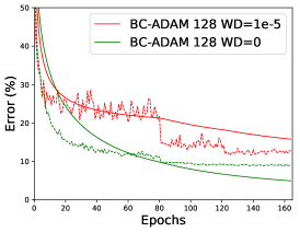
Refer to caption
(a) WD=1e-5 vs WD=0
Refer to caption
(b) |wbtwrt|superscriptsubscript𝑤𝑏𝑡superscriptsubscript𝑤𝑟𝑡|w_{b}^{t}-w_{r}^{t}|, WD=1e-5
Refer to caption
(c) |wbtwrt|superscriptsubscript𝑤𝑏𝑡superscriptsubscript𝑤𝑟𝑡|w_{b}^{t}-w_{r}^{t}|, WD=0
Figure 7: The effect of weight decay (WD) on BC-ADAM for training VGG-BC. The y-axis of (b) and (c) is the averaged weight difference between the binary weights wbsubscript𝑤𝑏w_{b} and the real-valued weights wrsubscript𝑤𝑟w_{r} , i.e., 1dwbtwrt11𝑑subscriptnormsuperscriptsubscript𝑤𝑏𝑡superscriptsubscript𝑤𝑟𝑡1\frac{1}{d}\|w_{b}^{t}-w_{r}^{t}\|_{1}. where d𝑑d is the number of weights in wbsubscript𝑤𝑏w_{b}.