On the Reality of the Wavefunction

Omid Charrakh Munich Center for Mathematical Philosophy, LMU Munich, Geschwister-Scholl-Platz 1, 80539 Munich (Germany) – omid.charrakh@campus.lmu.de.
Abstract

Within the Ontological Models Framework (OMF), Pusey, Barrett, and Rudolph (PBR) have given an argument by which they claimed that the epistemic view on the wavefunction should be ruled out. This study highlights an incorrect conclusion in PBR’s arguments, which was made due to inadequacies in the definitions of OMF. To be precise, OMF models the ontology of the preparation procedure, but it does not model the ontology of the measurement device. Such an asymmetric treatment becomes problematic, in scenarios in which measurement devices have a quantum nature. Modifying the OMF’s definition such that the ontology of the measurement device becomes included, we will see how PBR’s result disappears.

1 Introduction

In the foundations of quantum mechanics, the status of the wavefunction is one of the most debated issues. Associating a wavefunction with each system, QM provides very accurate predictions about the possible measurement outcomes. However, the axioms of QM are silent about the nature of the wavefunction, i.e., these axioms are logically consistent with several different ontological statuses of the wavefunction.

The Ontological Models Framework (OMF) introduced by Harrigan and Spekkens [1], is an attempt to provide a general formalism by which one can evaluate the ontology of the quantum theory and specifically the ontology of the wavefunction in realistic interpretations of QM.

Leifer explains [2] that one can choose one of the following three philosophical stands toward the wavefunction’s interpretation.

  1. 1.

    Antirealist Epistemic: Wavefunctions are epistemic, and there is not any deeper reality behind them.

  2. 2.

    Realist Epistemic: Wavefunctions are epistemic, but there is an underlying reality.

  3. 3.

    Realist Ontic: There is an underlying reality, and the wavefunctions correspond to the states of reality.

Options one and two are called ψ𝜓\psi-epistemic views. In these views, one interprets the wavefunction as a mathematical object which merely represents the agent’s knowledge of the quantum systems. Option three is referred to as the ψ𝜓\psi-ontic view, within which the wavefunction is considered to be a real object corresponding to an underlying reality of systems; such an object exists independently of the observer [3].

An important question is whether it is possible in principle to construct a realist ψ𝜓\psi-epistemic interpretation of QM (option two), or whether a realist is compelled to think ontologically about wavefunctions. PBR try to answer this question, and their answer is negative. In their famous article [4], PBR introduce an operational scenario whose statistics cannot be reproduced by ψ𝜓\psi-epistemic ontological models. PBR concluded that there is no way of having a realist epistemic interpretation of ψ𝜓\psi (option two); thus, the only remaining option for a realist is to choose option three.

The logical structure of the PBR’s argumentation can be expressed in the following way. There is a contradiction between the statistics of quantum theory (P1subscript𝑃1P_{1}) and the statistics of ψ𝜓\psi-epistemic ontological models (P2subscript𝑃2P_{2}) if one accepts a seemingly reasonable assumption about the ontological structure of the ontic states of a composite system, called the “Preparation Independence Postulate” (P3subscript𝑃3P_{3}). In general, these statements are going to be discussed within the ontological models framework (P4subscript𝑃4P_{4}).

QSTATP1ψepistemicP2PIPP3OMFP4subscript𝑄𝑆𝑇𝐴𝑇subscript𝑃1subscript𝜓𝑒𝑝𝑖𝑠𝑡𝑒𝑚𝑖𝑐subscript𝑃2subscript𝑃𝐼𝑃subscript𝑃3subscript𝑂𝑀𝐹subscript𝑃4bottom\underbrace{QSTAT}_{\text{$P_{1}$}}\hskip 5.69054pt\land\hskip 5.69054pt\underbrace{\psi-epistemic}_{\text{$P_{2}$}}\hskip 5.69054pt\land\underbrace{PIP}_{\text{$P_{3}$}}\hskip 5.69054pt\land\hskip 5.69054pt\underbrace{OMF}_{\text{$P_{4}$}}\hskip 5.69054pt\Rightarrow\hskip 5.69054pt\bot (1.1)

In confronting the above contradiction, so far, several arguments have been suggested aiming to put doubt on one (or even more than one) of the above propositions. Most of these suggestions can be classified into three categories.

  1. 1.

    Rejection of P1subscript𝑃1P_{1}. In this category, one can argue that maybe QM’s predictions are not always true. The idea of having null-measurements (measurements with no outcome) [5], or detection-inefficiency loophole [6] can be considered in this class.

  2. 2.

    Rejection of P2subscript𝑃2P_{2}. Another option is to accept the above contradiction, as a clue of a subtle constraint on accepting the ψ𝜓\psi-epistemic models. PBR themselves claimed that for a realist person, the only remaining option is to be a ψ𝜓\psi-ontologist [4].

  3. 3.

    Rejection of P3subscript𝑃3P_{3}. Most researchers have criticized the PIP assumption. Arguing that the two subsystems with a common past may share some ontic states in the present [7] or the idea that there may be some holistic properties of a composite system which cannot be reduced to its sub-systems [8], and several other arguments which can be found in [3], are examples of such criticisms.

  4. 4.

    Rejection of P4subscript𝑃4P_{4}. Except for the arguments from antirealists, who entirely reject the existence of an underlying reality behind the quantum states, there is no serious criticism of the PBR’s theorem which can be classified in this category. However, the argument provided in this study falls into this category.

This research highlights an incorrect conclusion in PBR’s arguments, which was made due to inadequacies in the definitions of OMF. To be precise, OMF models the ontology of the preparation procedure, but it does not model the ontology of the measurement device. Such an asymmetric treatment becomes problematic, in scenarios in which measurement devices have a quantum nature. Modifying the OMF definition so that we can insert the ontology of the measurement procedure into our analysis, we can see that PBR’s contradiction is not because of the ψ𝜓\psi-epistemic models. Rather, the problem is in the heart of our framework (OMF). I refer this modified version of the OMF as to “MOMF” (Modified Ontological Models Framework).

The order of the paper’s sections is as follows. A review of the OMF’s definitions and how they relate to the axioms of QM, as well as a precise description of PBR’s scenario in OMF, are provided in section two. Pointing out the problem of the ψ𝜓\psi-epistemic ontological models caused by OMF, the mathematical structure of the MOMF formalism followed by a statement of the PBR’s theorem within MOMF are discussed in section three. There, We will see how without using any further assumptions, the problem of the ψ𝜓\psi-epistemic models can be solved in MOMF. In conclusion, by reviewing all the mentioned ideas, it will be argued that PBR’s finding does not provide any implication for the nature of the wavefunction, rather what they have found shows us that we should be more careful about the way we model the ontology of QM.

2 OMF and the PBR Theorem

2.1 Operational QM

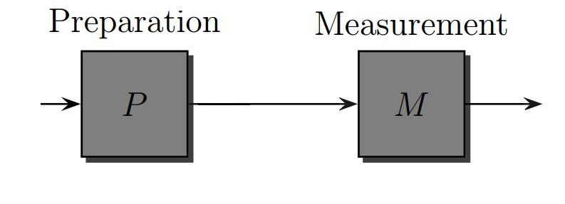
Consider an operational PM𝑃𝑀PM scenario, i.e., a scenario in which a system is prepared via a procedure/device P𝑃P, and then measured via a procedure/device M𝑀M. In this situation, the interaction between the prepared system and the measurement device results in an outcome for which QM provides us the associated probability of finding that outcome. Figure (1) depicts such a scenario. According to QM, we can express the following axioms for describing such a situation.
Refer to caption
Figure 1: The schematic of an operational PM𝑃𝑀PM scenario. A preparation device P𝑃P, prepares a state which is supposed to be measured via a measurement device M𝑀M.
Definition 2.1.

Operational QM posits the following two axioms to describe a PMPMPM scenario [9].

Axiom 2.1 (Preparation).

A preparation P𝑃P is associated to a trace one positive operator ρ𝜌\rho, known as the density operator, acting on the Hilbert space \mathcal{H}.

Axiom 2.2 (Measurement).

A measurement M𝑀M is associated with a positive operator valued measure (POVM) {Mm}subscript𝑀𝑚\{M_{m}\} such that mMm=Isubscript𝑚subscript𝑀𝑚𝐼\sum_{m}{M_{m}}=I.

Finally, the probability of a measurement M𝑀M yielding outcome m𝑚m, given a preparation procedure P𝑃P, is

pr(mP,M)=Tr(Mmρ).𝑝𝑟conditional𝑚𝑃𝑀𝑇𝑟subscript𝑀𝑚𝜌pr(m\mid P,M)=Tr(M_{m}\rho). (2.1)

2.2 Ontological Models Framework

To investigate the ontological status of ψ𝜓\psi, one needs an ontological framework. Such a framework cannot be inferred directly from the axioms of QM. What we can do, is to look for an ontological model whose structure is constrained by the fact that the predictions of the ontological model and the operational ones, should be equal. In 2007, Harrigan and Spekkens proposed a framework called “Ontological Models Framework (OMF)” [1] aiming to provide the most general formalism for realistic interpretations of quantum scenarios.

The basic idea of OMF is to associate an ontic state space Λ={λi}Λsubscript𝜆𝑖\Lambda=\{\lambda_{i}\} with each physical system. This space is supposed to be the space of all the possible ontic states λisubscript𝜆𝑖\lambda_{i} of a system in the sense that the ontic states are the real states of a system which are independent of our observation, information and what so ever. Following [1], we have the following three definitions.

Definition 2.2.

OMF posits an ontic state space ΛΛ\Lambda and prescribes a probability distribution over ΛΛ\Lambda for every preparation procedure PPP, denoted by a density function pr(λP)prconditionalλPpr(\lambda\mid P), and a probability distribution over the different outcomes MmsubscriptMmM_{m} of a measurement MMM for every ontic state λΛλΛ\lambda\in\Lambda, denoted by a response function pr(mλ,M)prconditionalmλMpr(m\mid\lambda,M). Finally, for all PPP and MMM, it must satisfy the conditions

Λpr(λP)𝑑λ=1subscriptΛ𝑝𝑟conditional𝜆𝑃differential-d𝜆1\int_{\Lambda}pr(\lambda\mid P)d\lambda=1 (2.2)
mpr(mλ,M)=1subscript𝑚𝑝𝑟conditional𝑚𝜆𝑀1\sum_{m}{pr(m\mid\lambda,M)}=1 (2.3)
Λpr(λP)pr(mλ,M)𝑑λ=pr(mP,M)=Tr(Mmρ)subscriptΛ𝑝𝑟conditional𝜆𝑃𝑝𝑟conditional𝑚𝜆𝑀differential-d𝜆𝑝𝑟conditional𝑚𝑃𝑀𝑇𝑟subscript𝑀𝑚𝜌\int_{\Lambda}pr(\lambda\mid P)pr(m\mid\lambda,M)d\lambda=pr(m\mid P,M)=Tr(M_{m}\rho) (2.4)

where ρ𝜌\rho is the density operator associated with P𝑃P and Mmsubscript𝑀𝑚M_{m} is the POVM element associated with the m𝑚m-th outcome of measurement M𝑀M.

The idea of OMF is straightforward; As an operational theory, quantum theory associates an operational state ρ𝜌\rho with each preparation procedure. But, since we are not sure whether ρ𝜌\rho is the system’s ontic state (λ𝜆\lambda) or not, we should simulate the ontic level of ρ𝜌\rho by the expression pr(λP)𝑝𝑟conditional𝜆𝑃pr(\lambda\mid P). After this simulation, the probabilities of finding different measurement outcomes will depend on the ontic states of the preparation procedure, expressed by pr(mλ,M)𝑝𝑟conditional𝑚𝜆𝑀pr(m\mid\lambda,M). This implies that the outcomes’ probabilities depend on the measurement procedure M𝑀M and the ontic state λ𝜆\lambda. Finally, these probabilities should be summed over all the relevant ontic states.

Definition 2.3.

An ontological model is ψ𝜓\psi-ontic if for any pair of preparation procedures, Pψ1subscript𝑃subscript𝜓1P_{\psi_{1}} and Pψ2subscript𝑃subscript𝜓2P_{\psi_{2}}, associated with distinct (and non-degenerate) quantum states ψ1subscript𝜓1\psi_{1} and ψ2subscript𝜓2\psi_{2}, we have pr(λPψ1)pr(λPψ2)=0𝑝𝑟conditional𝜆subscript𝑃subscript𝜓1𝑝𝑟conditional𝜆subscript𝑃subscript𝜓20pr(\lambda\mid P_{\psi_{1}})pr(\lambda\mid P_{\psi_{2}})=0 for all λΛ𝜆Λ\lambda\in\Lambda.

Definition 2.4.

If an ontological model fails to be ψ𝜓\psi-ontic, then it is said to be ψ𝜓\psi-epistemic.

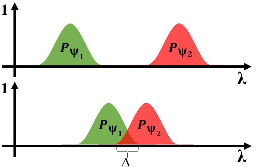
The upper graph of figure (2) depicts the ontic state space of a ψ𝜓\psi-ontic ontological model, in which, there is no shared λ𝜆\lambda between two preparation procedures. The lower graph shows a ψ𝜓\psi-epistemic ontological model. In ψ𝜓\psi-ontic models, two operationally distinct states (say |x+ketlimit-from𝑥\ket{x+} and |z+ketlimit-from𝑧\ket{z+}) are ontologically distinct too. In ψ𝜓\psi-epistemic models, there exists (at least) one ontic state which is compatible with two different operational states.
Refer to caption
Figure 2: A demonstration of ψ𝜓\psi-ontic (upper graph) and ψ𝜓\psi-epistemic (lower graph) ontological models. In ψ𝜓\psi-epistemic models, the common support of ontic states has a non-zero measure.

So far, all of our statements about OMF have considered the single-party PM𝑃𝑀PM scenarios (a single system is assumed to be prepared and then measured). In this sense, OMF aims to provide the most general ontological structure behind the operational PM𝑃𝑀PM scenario. However, most of the problematic scenarios in foundations of QM are multipartite ones. For instance, the Bell and the PBR scenarios are both about two systems which are going to be joined to create a single composite system.

Proposition 2.1.

For systems A𝐴A and B𝐵B whose hypothetical composite system AB𝐴𝐵AB is (operationally) prepared and measured by PABsubscript𝑃𝐴𝐵P_{AB} and MABsuperscript𝑀𝐴𝐵M^{AB}, bipartite OMF posits an ontic state space ΛABsubscriptΛ𝐴𝐵\Lambda_{AB} and prescribes a probability distribution over ΛABsubscriptΛ𝐴𝐵\Lambda_{AB} for every preparation procedure PABsubscript𝑃𝐴𝐵P_{AB}, denoted by a density function pr(λABPAB)𝑝𝑟conditionalsubscript𝜆𝐴𝐵subscript𝑃𝐴𝐵pr(\lambda_{AB}\mid P_{AB}), and a probability distribution over the different outcomes mABsuperscript𝑚𝐴𝐵m^{AB} of a measurement MABsuperscript𝑀𝐴𝐵M^{AB} for every ontic state λABΛABsubscript𝜆𝐴𝐵subscriptΛ𝐴𝐵\lambda_{AB}\in\Lambda_{AB}, denoted by a response function pr(mABλAB,MAB)𝑝𝑟conditionalsuperscript𝑚𝐴𝐵subscript𝜆𝐴𝐵superscript𝑀𝐴𝐵pr(m^{AB}\mid\lambda_{AB},M^{AB}). Finally, for all PABsubscript𝑃𝐴𝐵P_{AB} and MABsuperscript𝑀𝐴𝐵M^{AB}, it will satisfy the following three conditions

ΛABpr(λABPAB)𝑑λAB=1subscriptsubscriptΛ𝐴𝐵𝑝𝑟conditionalsubscript𝜆𝐴𝐵subscript𝑃𝐴𝐵differential-dsubscript𝜆𝐴𝐵1\int_{\Lambda_{AB}}pr(\lambda_{AB}\mid P_{AB})d\lambda_{AB}=1 (2.5)
mABpr(mABλAB,MAB)=1subscriptsuperscript𝑚𝐴𝐵𝑝𝑟conditionalsuperscript𝑚𝐴𝐵subscript𝜆𝐴𝐵superscript𝑀𝐴𝐵1\sum_{m^{AB}}{pr(m^{AB}\mid\lambda_{AB},M^{AB})}=1 (2.6)
ΛABpr(λABPAB)pr(mABλAB,MAB)𝑑λAB=pr(mABPAB,MAB)=Tr(MmABρAB)subscriptsubscriptΛ𝐴𝐵𝑝𝑟conditionalsubscript𝜆𝐴𝐵subscript𝑃𝐴𝐵𝑝𝑟conditionalsuperscript𝑚𝐴𝐵subscript𝜆𝐴𝐵superscript𝑀𝐴𝐵differential-dsubscript𝜆𝐴𝐵𝑝𝑟conditionalsuperscript𝑚𝐴𝐵subscript𝑃𝐴𝐵superscript𝑀𝐴𝐵𝑇𝑟subscriptsuperscript𝑀𝐴𝐵𝑚subscript𝜌𝐴𝐵\int_{\Lambda_{AB}}pr(\lambda_{AB}\mid P_{AB})pr(m^{AB}\mid\lambda_{AB},M^{AB})d\lambda_{AB}=pr(m^{AB}\mid P_{AB},M^{AB})=Tr(M^{AB}_{m}\rho_{AB}) (2.7)

where ρABsubscript𝜌𝐴𝐵\rho_{AB} is the density operator associated with PABsubscript𝑃𝐴𝐵P_{AB} and MmABsubscriptsuperscript𝑀𝐴𝐵𝑚M^{AB}_{m} is the POVM element associated with the m𝑚m-th outcome of measurement MABsuperscript𝑀𝐴𝐵M^{AB}.

Proof.

This proposition is derivable from the axioms of operational QM, plus the OMF definition. Consider two systems A𝐴A and B𝐵B, for which we don’t know anything regarding their preparation and measurement procedures. According to the OMF definition, define an ontological model for their “single” composite system AB𝐴𝐵AB. ∎

Definition 2.5.

Consider two pure states, ψAsubscript𝜓𝐴\psi_{A} and ψBsubscript𝜓𝐵\psi_{B}, prepared independently at two space-like separated points. From the OMF definition, these operational states correspond to the ontic states λAΛAsubscript𝜆𝐴subscriptΛ𝐴\lambda_{A}\in\Lambda_{A} and λBΛBsubscript𝜆𝐵subscriptΛ𝐵\lambda_{B}\in\Lambda_{B}, respectively. If we combine these two systems to create the composite system AB𝐴𝐵AB, which is described operationally by ψAB=ψAψBsubscript𝜓𝐴𝐵tensor-productsubscript𝜓𝐴subscript𝜓𝐵\psi_{AB}=\psi_{A}\otimes\psi_{B}, the Preparation Independence Postulate (PIP in OMF) assumes that the ontic state of this composite system can be modeled in the following way.

ΛAB=ΛA×ΛBλAB=(λA,λB)subscriptΛ𝐴𝐵subscriptΛ𝐴subscriptΛ𝐵subscript𝜆𝐴𝐵subscript𝜆𝐴subscript𝜆𝐵\Lambda_{AB}=\Lambda_{A}\times\Lambda_{B}\equiv\lambda_{AB}=(\lambda_{A},\lambda_{B}) (2.8)
pr(λABψAB)=pr(λAψA)pr(λBψB)𝑝𝑟conditionalsubscript𝜆𝐴𝐵subscript𝜓𝐴𝐵𝑝𝑟conditionalsubscript𝜆𝐴subscript𝜓𝐴𝑝𝑟conditionalsubscript𝜆𝐵subscript𝜓𝐵pr(\lambda_{AB}\mid\psi_{AB})=pr(\lambda_{A}\mid\psi_{A})pr(\lambda_{B}\mid\psi_{B}) (2.9)

where λABΛABsubscript𝜆𝐴𝐵subscriptΛ𝐴𝐵\lambda_{AB}\in\Lambda_{AB} is the ontic state of the composite system AB𝐴𝐵AB.

2.3 The PBR Theorem in OMF

Imagine Alice and Bob are living in two space-like separated regions, and they prepare their quantum states via the preparation procedures PAsubscript𝑃𝐴P_{A} and PBsubscript𝑃𝐵P_{B} such that there is not any operational correlation between these two processes. In the original example of PBR, Alice can choose to prepare her state in either |0Aketsubscript0𝐴\ket{0_{A}} or |+Aketsubscript𝐴\ket{+_{A}}. Similarly, Bob can prepare his state in either |0Bketsubscript0𝐵\ket{0_{B}} or |+Bketsubscript𝐵\ket{+_{B}} (PBR express these statements, by demanding two copies of the same prepared system).

According to figure (2), an arbitrary ψ𝜓\psi-epistemic ontological model implies that Alice and Bob have the overlaps ΔAsubscriptΔ𝐴\Delta_{A} and ΔBsubscriptΔ𝐵\Delta_{B} in the probability distributions over their ontic state spaces ΛAsubscriptΛ𝐴\Lambda_{A} and ΛBsubscriptΛ𝐵\Lambda_{B}. Since these people are living in two space-like separated regions, there is not any operational correlation between their preparation procedures. Hence, according to the operational QM the following relation holds,

ψAB=ψAψB.subscript𝜓𝐴𝐵tensor-productsubscript𝜓𝐴subscript𝜓𝐵\psi_{AB}=\psi_{A}\otimes\psi_{B}. (2.10)

So, there are four possibilities for preparing the composite system AB,

ψAB{ψAB1,ψAB2,ψAB3,ψAB4}subscript𝜓𝐴𝐵subscriptsuperscript𝜓1𝐴𝐵subscriptsuperscript𝜓2𝐴𝐵subscriptsuperscript𝜓3𝐴𝐵subscriptsuperscript𝜓4𝐴𝐵\psi_{AB}\in\{\psi^{1}_{AB},\psi^{2}_{AB},\psi^{3}_{AB},\psi^{4}_{AB}\} (2.11)

where ψAB1=|0A|0Bsubscriptsuperscript𝜓1𝐴𝐵tensor-productketsubscript0𝐴ketsubscript0𝐵\psi^{1}_{AB}=\ket{0_{A}}\otimes\ket{0_{B}}, ψAB2=|0A|+Bsubscriptsuperscript𝜓2𝐴𝐵tensor-productketsubscript0𝐴ketsubscript𝐵\psi^{2}_{AB}=\ket{0_{A}}\otimes\ket{+_{B}}, ψAB3=|+A|0Bsubscriptsuperscript𝜓3𝐴𝐵tensor-productketsubscript𝐴ketsubscript0𝐵\psi^{3}_{AB}=\ket{+_{A}}\otimes\ket{0_{B}} and ψAB4=|+A|+Bsubscriptsuperscript𝜓4𝐴𝐵tensor-productketsubscript𝐴ketsubscript𝐵\psi^{4}_{AB}=\ket{+_{A}}\otimes\ket{+_{B}}.

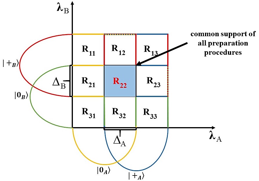
As it can be seen in figure (3), in general, the support of the composite ontic state λABsubscript𝜆𝐴𝐵\lambda_{AB} is composed of nine mutually exclusive sub-regions.

supp(λABψAB)=R11\sqcupdotR12\sqcupdot\sqcupdotR33𝑠𝑢𝑝𝑝conditionalsubscript𝜆𝐴𝐵subscript𝜓𝐴𝐵subscript𝑅11\sqcupdotsubscript𝑅12\sqcupdot\sqcupdotsubscript𝑅33supp(\lambda_{AB}\mid\psi_{AB})=R_{11}\sqcupdot R_{12}\sqcupdot...\sqcupdot R_{33} (2.12)

Also, note that corresponding to each operational state ψABisubscriptsuperscript𝜓𝑖𝐴𝐵\psi^{i}_{AB} there exists a particular region of ΛABsubscriptΛ𝐴𝐵\Lambda_{AB}, to which the ontic state λABsubscript𝜆𝐴𝐵\lambda_{AB} will be restricted. For instance, if the composite system has been prepared in ψAB1=|0A|0Bsubscriptsuperscript𝜓1𝐴𝐵tensor-productketsubscript0𝐴ketsubscript0𝐵\psi^{1}_{AB}=\ket{0_{A}}\otimes\ket{0_{B}}, one can infer that Alice and Bob have prepared their systems in |0Aketsubscript0𝐴\ket{0_{A}} and |0Bketsubscript0𝐵\ket{0_{B}}, respectively. In this situation, λABsubscript𝜆𝐴𝐵\lambda_{AB} will be restricted to the region R31\sqcupdotR32\sqcupdotR21\sqcupdotR22subscript𝑅31\sqcupdotsubscript𝑅32\sqcupdotsubscript𝑅21\sqcupdotsubscript𝑅22R_{31}\sqcupdot R_{32}\sqcupdot R_{21}\sqcupdot R_{22}. In general, we have the following four formulas.

{supp(λABψAB1)=R21\sqcupdotR22\sqcupdotR31\sqcupdotR32supp(λABψAB2)=R11\sqcupdotR12\sqcupdotR21\sqcupdotR22supp(λABψAB3)=R22\sqcupdotR23\sqcupdotR32\sqcupdotR33supp(λABψAB4)=R12\sqcupdotR13\sqcupdotR22\sqcupdotR23cases𝑠𝑢𝑝𝑝conditionalsubscript𝜆𝐴𝐵subscriptsuperscript𝜓1𝐴𝐵subscript𝑅21\sqcupdotsubscript𝑅22\sqcupdotsubscript𝑅31\sqcupdotsubscript𝑅32otherwise𝑠𝑢𝑝𝑝conditionalsubscript𝜆𝐴𝐵subscriptsuperscript𝜓2𝐴𝐵subscript𝑅11\sqcupdotsubscript𝑅12\sqcupdotsubscript𝑅21\sqcupdotsubscript𝑅22otherwise𝑠𝑢𝑝𝑝conditionalsubscript𝜆𝐴𝐵subscriptsuperscript𝜓3𝐴𝐵subscript𝑅22\sqcupdotsubscript𝑅23\sqcupdotsubscript𝑅32\sqcupdotsubscript𝑅33otherwise𝑠𝑢𝑝𝑝conditionalsubscript𝜆𝐴𝐵subscriptsuperscript𝜓4𝐴𝐵subscript𝑅12\sqcupdotsubscript𝑅13\sqcupdotsubscript𝑅22\sqcupdotsubscript𝑅23otherwise\begin{cases}supp(\lambda_{AB}\mid\psi^{1}_{AB})=R_{21}\sqcupdot R_{22}\sqcupdot R_{31}\sqcupdot R_{32}\\ supp(\lambda_{AB}\mid\psi^{2}_{AB})=R_{11}\sqcupdot R_{12}\sqcupdot R_{21}\sqcupdot R_{22}\\ supp(\lambda_{AB}\mid\psi^{3}_{AB})=R_{22}\sqcupdot R_{23}\sqcupdot R_{32}\sqcupdot R_{33}\\ supp(\lambda_{AB}\mid\psi^{4}_{AB})=R_{12}\sqcupdot R_{13}\sqcupdot R_{22}\sqcupdot R_{23}\\ \end{cases} (2.13)

From the above equations, it is evident that R22subscript𝑅22R_{22} is the only region of ΛABsubscriptΛ𝐴𝐵\Lambda_{AB} which is repeating in all of the four equations. This means that R22subscript𝑅22R_{22} is compatible with all of the four possible preparation procedures of ψABsubscript𝜓𝐴𝐵\psi_{AB}.

While the first assumption of PIP (2.8) implies that R22=ΔA×ΔBsubscript𝑅22subscriptΔ𝐴subscriptΔ𝐵R_{22}=\Delta_{A}\times\Delta_{B}, its second assumption (2.9) implies that the ontic state λAB=(λA,λB)subscript𝜆𝐴𝐵subscript𝜆𝐴subscript𝜆𝐵\lambda_{AB}=(\lambda_{A},\lambda_{B}) of each run of the experiment will be chosen from R22subscript𝑅22R_{22} with the non-zero probability q=|ΔA×ΔB||supp(λABψAB)|>0q=\frac{|\Delta_{A}\times\Delta_{B}|}{|supp(\lambda_{AB}\mid\psi_{AB})|}>0. As we will see in the next pages, ψ𝜓\psi-epistemic models cannot reproduce PBR statistics because of the appearance of R22subscript𝑅22R_{22}. In other words, R22subscript𝑅22R_{22} is a problematic region in ψ𝜓\psi-epistemic models.

So far, we have reviewed many details of PBR preparation procedure. Before explicitly expressing the main theorem, PBR measurement procedure should also be known. PBR define their measurement procedure to be MAB={M1AB,M2AB,M3AB,M4AB}superscript𝑀𝐴𝐵subscriptsuperscript𝑀𝐴𝐵1subscriptsuperscript𝑀𝐴𝐵2subscriptsuperscript𝑀𝐴𝐵3subscriptsuperscript𝑀𝐴𝐵4M^{AB}=\{M^{AB}_{1},M^{AB}_{2},M^{AB}_{3},M^{AB}_{4}\}, which is defined as follows.

M1AB=12(|0A|1B+|1A|0B)subscriptsuperscript𝑀𝐴𝐵112ketsubscript0𝐴ketsubscript1𝐵ketsubscript1𝐴ketsubscript0𝐵\displaystyle M^{AB}_{1}=\frac{1}{\sqrt{2}}(\Ket{0_{A}}\Ket{1_{B}}+\Ket{1_{A}}\Ket{0_{B}}) (2.14)
M2AB=12(|0A|B+|1A|+B)subscriptsuperscript𝑀𝐴𝐵212ketsubscript0𝐴ketsubscript𝐵ketsubscript1𝐴ketsubscript𝐵\displaystyle M^{AB}_{2}=\frac{1}{\sqrt{2}}(\Ket{0_{A}}\Ket{-_{B}}+\Ket{1_{A}}\Ket{+_{B}})
M3AB=12(|+A|1B+|A|0B)subscriptsuperscript𝑀𝐴𝐵312ketsubscript𝐴ketsubscript1𝐵ketsubscript𝐴ketsubscript0𝐵\displaystyle M^{AB}_{3}=\frac{1}{\sqrt{2}}(\Ket{+_{A}}\Ket{1_{B}}+\Ket{-_{A}}\Ket{0_{B}})
M4AB=12(|+A|B+|A|+B)subscriptsuperscript𝑀𝐴𝐵412ketsubscript𝐴ketsubscript𝐵ketsubscript𝐴ketsubscript𝐵\displaystyle M^{AB}_{4}=\frac{1}{\sqrt{2}}(\Ket{+_{A}}\Ket{-_{B}}+\Ket{-_{A}}\Ket{+_{B}})

It can be verified that elements of the above set constitute a complete, two-by-two orthogonal basis corresponding to four possible outcomes of a measurement device MABsuperscript𝑀𝐴𝐵M^{AB}. This measurement procedure is entangled, meaning that the elements of this set cannot be separated into two parts, MiAB(MiA,MiB)subscriptsuperscript𝑀𝐴𝐵𝑖subscriptsuperscript𝑀𝐴𝑖subscriptsuperscript𝑀𝐵𝑖M^{AB}_{i}\neq(M^{A}_{i},M^{B}_{i}).

Theorem 2.1 (PBR Theorem).

Assuming PIP, the (operational) PBR scenario cannot be (ontologically) reproduced by ψ𝜓\psi-epistemic ontological models.

Proof.

To clearly show that PBR’s scenario is not reproducible by any ψ𝜓\psi-epistemic ontological models, let us express the arguments step-by-step.

Step 1. Consider a ψ𝜓\psi-epistemic ontological model which is supposed to reproduce our operational statistics. Placing the PIP assumption in proposition (2.1) results in the following equations for the PBR composite system.

p𝑝\displaystyle p r(mABPAB,MAB)=Tr(MmABρAB)=𝑟conditionalsuperscript𝑚𝐴𝐵subscript𝑃𝐴𝐵superscript𝑀𝐴𝐵𝑇𝑟subscriptsuperscript𝑀𝐴𝐵𝑚subscript𝜌𝐴𝐵absent\displaystyle r(m^{AB}\mid P_{AB},M^{AB})=Tr(M^{AB}_{m}\rho_{AB})= (2.15)
ΛABsubscriptsubscriptΛ𝐴𝐵\displaystyle\int_{\Lambda_{AB}} dλABpr(λABPAB)pr(mABλAB,MAB)=𝑑subscript𝜆𝐴𝐵𝑝𝑟conditionalsubscript𝜆𝐴𝐵subscript𝑃𝐴𝐵𝑝𝑟conditionalsuperscript𝑚𝐴𝐵subscript𝜆𝐴𝐵superscript𝑀𝐴𝐵absent\displaystyle d\lambda_{AB}pr(\lambda_{AB}\mid P_{AB})pr(m^{AB}\mid\lambda_{AB},M^{AB})=
ΛAΛBsubscriptsubscriptΛ𝐴subscriptsubscriptΛ𝐵\displaystyle\int_{\Lambda_{A}}\int_{\Lambda_{B}} dλAdλBpr(λAPA)pr(λBPB)pr(mABMAB,λA,λB)𝑑subscript𝜆𝐴𝑑subscript𝜆𝐵𝑝𝑟conditionalsubscript𝜆𝐴subscript𝑃𝐴𝑝𝑟conditionalsubscript𝜆𝐵subscript𝑃𝐵𝑝𝑟conditionalsuperscript𝑚𝐴𝐵superscript𝑀𝐴𝐵subscript𝜆𝐴subscript𝜆𝐵\displaystyle d\lambda_{A}d\lambda_{B}pr(\lambda_{A}\mid P_{A})pr(\lambda_{B}\mid P_{B})pr(m^{AB}\mid M^{AB},\lambda_{A},\lambda_{B})
Refer to caption
Figure 3: The ontic state space ΛABsubscriptΛ𝐴𝐵\Lambda_{AB} of an arbitrary ψ𝜓\psi-epistemic ontological model. In general, the ontic state λABsubscript𝜆𝐴𝐵\lambda_{AB} can be chosen from nine non-overlapped regions. The states coming from the common region R22=ΔA×ΔBsubscript𝑅22subscriptΔ𝐴subscriptΔ𝐵R_{22}=\Delta_{A}\times\Delta_{B} are compatible with all the four possible preparation procedures.

Step 2. Our ontological model must be able to reproduce compatible statistics with the following two observations.

Observation 1: The measurement device can select only the outcomes which are not orthogonal to the prepared state. So the probability of choosing an outcome which is orthogonal to the prepared state is zero. This observation leads to four equations at the operational level of QM.

operational level{pr(mAB=1ψAB=|0A0B,MAB)=Tr(M1ABρAB1)=0pr(mAB=2ψAB=|0A+B,MAB)=Tr(M2ABρAB2)=0pr(mAB=3ψAB=|+A0B,MAB)=Tr(M3ABρAB3)=0pr(mAB=4ψAB=|+A+B,MAB)=Tr(M4ABρAB4)=0\textup{operational level}\begin{cases}pr(m^{AB}=1\mid\psi_{AB}=\ket{0_{A}0_{B}},M^{AB})=Tr(M^{AB}_{1}\rho^{1}_{AB})=0\\ pr(m^{AB}=2\mid\psi_{AB}=\ket{0_{A}+_{B}},M^{AB})=Tr(M^{AB}_{2}\rho^{2}_{AB})=0\\ pr(m^{AB}=3\mid\psi_{AB}=\ket{+_{A}0_{B}},M^{AB})=Tr(M^{AB}_{3}\rho^{3}_{AB})=0\\ pr(m^{AB}=4\mid\psi_{AB}=\ket{+_{A}+_{B}},M^{AB})=Tr(M^{AB}_{4}\rho^{4}_{AB})=0\\ \end{cases} (2.16)

where ρAB1=|0A0B0A0B|subscriptsuperscript𝜌1𝐴𝐵subscript0𝐴subscript0𝐵subscript0𝐴subscript0𝐵\rho^{1}_{AB}=\outerproduct{0_{A}0_{B}}{0_{A}0_{B}}, ρAB2=|0A+B0A+B|subscriptsuperscript𝜌2𝐴𝐵limit-fromsubscript0𝐴subscript𝐵limit-fromsubscript0𝐴subscript𝐵\rho^{2}_{AB}=\outerproduct{0_{A}+_{B}}{0_{A}+_{B}}, ρAB3=|+A0B+A0B|subscriptsuperscript𝜌3𝐴𝐵subscript𝐴subscript0𝐵subscript𝐴subscript0𝐵\rho^{3}_{AB}=\outerproduct{+_{A}0_{B}}{+_{A}0_{B}}, and ρAB4=|+A+B+A+B|subscriptsuperscript𝜌4𝐴𝐵subscript𝐴subscript𝐵subscript𝐴subscript𝐵\rho^{4}_{AB}=\outerproduct{+_{A}+_{B}}{+_{A}+_{B}}.

Combining the above results with equation (2.15), one can convert this set of four operational equations into the following set of equations at the ontic level of QM.

ontic level{pr(mAB=1λA,λB,MAB)=0,whenψAB=|0A0Bpr(mAB=2λA,λB,MAB)=0,whenψAB=|0A+Bpr(mAB=3λA,λB,MAB)=0,whenψAB=|+A0Bpr(mAB=4λA,λB,MAB)=0,whenψAB=|+A+Bontic levelcasesformulae-sequence𝑝𝑟superscript𝑚𝐴𝐵conditional1subscript𝜆𝐴subscript𝜆𝐵superscript𝑀𝐴𝐵0𝑤𝑒𝑛subscript𝜓𝐴𝐵ketsubscript0𝐴subscript0𝐵otherwiseformulae-sequence𝑝𝑟superscript𝑚𝐴𝐵conditional2subscript𝜆𝐴subscript𝜆𝐵superscript𝑀𝐴𝐵0𝑤𝑒𝑛subscript𝜓𝐴𝐵ketlimit-fromsubscript0𝐴subscript𝐵otherwiseformulae-sequence𝑝𝑟superscript𝑚𝐴𝐵conditional3subscript𝜆𝐴subscript𝜆𝐵superscript𝑀𝐴𝐵0𝑤𝑒𝑛subscript𝜓𝐴𝐵ketsubscript𝐴subscript0𝐵otherwiseformulae-sequence𝑝𝑟superscript𝑚𝐴𝐵conditional4subscript𝜆𝐴subscript𝜆𝐵superscript𝑀𝐴𝐵0𝑤𝑒𝑛subscript𝜓𝐴𝐵ketsubscript𝐴subscript𝐵otherwise\textup{ontic level}\begin{cases}pr(m^{AB}=1\mid\lambda_{A},\lambda_{B},M^{AB})=0,\hskip 5.69054ptwhen\hskip 5.69054pt\psi_{AB}=\ket{0_{A}0_{B}}\\ pr(m^{AB}=2\mid\lambda_{A},\lambda_{B},M^{AB})=0,\hskip 5.69054ptwhen\hskip 5.69054pt\psi_{AB}=\ket{0_{A}+_{B}}\\ pr(m^{AB}=3\mid\lambda_{A},\lambda_{B},M^{AB})=0,\hskip 5.69054ptwhen\hskip 5.69054pt\psi_{AB}=\ket{+_{A}0_{B}}\\ pr(m^{AB}=4\mid\lambda_{A},\lambda_{B},M^{AB})=0,\hskip 5.69054ptwhen\hskip 5.69054pt\psi_{AB}=\ket{+_{A}+_{B}}\end{cases} (2.17)

Also, as explained in (2.13), each preparation procedure of the composite system corresponds to a particular part of ΛABsubscriptΛ𝐴𝐵\Lambda_{AB}. Hence, domains of the last set of equations are as follows.

ontic level{pr(mAB=1λA,λB,MAB)=0,whenλABR21\sqcupdotR22\sqcupdotR31\sqcupdotR32pr(mAB=2λA,λB,MAB)=0,whenλABR11\sqcupdotR12\sqcupdotR21\sqcupdotR22pr(mAB=3λA,λB,MAB)=0,whenλABR22\sqcupdotR23\sqcupdotR32\sqcupdotR33pr(mAB=4λA,λB,MAB)=0,whenλABR12\sqcupdotR13\sqcupdotR22\sqcupdotR23ontic levelcasesformulae-sequence𝑝𝑟superscript𝑚𝐴𝐵conditional1subscript𝜆𝐴subscript𝜆𝐵superscript𝑀𝐴𝐵0𝑤𝑒𝑛subscript𝜆𝐴𝐵subscript𝑅21\sqcupdotsubscript𝑅22\sqcupdotsubscript𝑅31\sqcupdotsubscript𝑅32otherwiseformulae-sequence𝑝𝑟superscript𝑚𝐴𝐵conditional2subscript𝜆𝐴subscript𝜆𝐵superscript𝑀𝐴𝐵0𝑤𝑒𝑛subscript𝜆𝐴𝐵subscript𝑅11\sqcupdotsubscript𝑅12\sqcupdotsubscript𝑅21\sqcupdotsubscript𝑅22otherwiseformulae-sequence𝑝𝑟superscript𝑚𝐴𝐵conditional3subscript𝜆𝐴subscript𝜆𝐵superscript𝑀𝐴𝐵0𝑤𝑒𝑛subscript𝜆𝐴𝐵subscript𝑅22\sqcupdotsubscript𝑅23\sqcupdotsubscript𝑅32\sqcupdotsubscript𝑅33otherwiseformulae-sequence𝑝𝑟superscript𝑚𝐴𝐵conditional4subscript𝜆𝐴subscript𝜆𝐵superscript𝑀𝐴𝐵0𝑤𝑒𝑛subscript𝜆𝐴𝐵subscript𝑅12\sqcupdotsubscript𝑅13\sqcupdotsubscript𝑅22\sqcupdotsubscript𝑅23otherwise\textup{ontic level}\begin{cases}pr(m^{AB}=1\mid\lambda_{A},\lambda_{B},M^{AB})=0,\hskip 5.69054ptwhen\hskip 5.69054pt\lambda_{AB}\in R_{21}\sqcupdot{\color[rgb]{1,0,0}\definecolor[named]{pgfstrokecolor}{rgb}{1,0,0}R_{22}}\sqcupdot R_{31}\sqcupdot R_{32}\\ pr(m^{AB}=2\mid\lambda_{A},\lambda_{B},M^{AB})=0,\hskip 5.69054ptwhen\hskip 5.69054pt\lambda_{AB}\in R_{11}\sqcupdot R_{12}\sqcupdot R_{21}\sqcupdot{\color[rgb]{1,0,0}\definecolor[named]{pgfstrokecolor}{rgb}{1,0,0}R_{22}}\\ pr(m^{AB}=3\mid\lambda_{A},\lambda_{B},M^{AB})=0,\hskip 5.69054ptwhen\hskip 5.69054pt\lambda_{AB}\in{\color[rgb]{1,0,0}\definecolor[named]{pgfstrokecolor}{rgb}{1,0,0}R_{22}}\sqcupdot R_{23}\sqcupdot R_{32}\sqcupdot R_{33}\\ pr(m^{AB}=4\mid\lambda_{A},\lambda_{B},M^{AB})=0,\hskip 5.69054ptwhen\hskip 5.69054pt\lambda_{AB}\in R_{12}\sqcupdot R_{13}\sqcupdot{\color[rgb]{1,0,0}\definecolor[named]{pgfstrokecolor}{rgb}{1,0,0}R_{22}}\sqcupdot R_{23}\\ \end{cases} (2.18)

Observation 2: According to equation (2.6), regardless of which quantum state has been prepared, the sum of the response functions must be equal to one.

Σi=14pr(mAB=iλA,λB,MAB)=1subscriptsuperscriptΣ4𝑖1𝑝𝑟superscript𝑚𝐴𝐵conditional𝑖subscript𝜆𝐴subscript𝜆𝐵superscript𝑀𝐴𝐵1\Sigma^{4}_{i=1}{pr(m^{AB}=i\mid\lambda_{A},\lambda_{B},M^{AB})}=1 (2.19)

Step 3. In this step, we check whether our model can satisfy our observations, in equations (2.18) and (2.19), consistently or not. First of all, remember that in ψ𝜓\psi-epistemic models the ontic state λABsubscript𝜆𝐴𝐵\lambda_{AB} comes from the the overlap region R22=ΔA×ΔBsubscript𝑅22subscriptΔ𝐴subscriptΔ𝐵R_{22}=\Delta_{A}\times\Delta_{B} at q=|ΔA×ΔB||supp(λABψAB)|q=\frac{|\Delta_{A}\times\Delta_{B}|}{|supp(\lambda_{AB}\mid\psi_{AB})|} of the times. Hence, regardless of which preparation procedure will be chosen by Alice and Bob, there is always the possibility of having the ontic states being in this region λABΔA×ΔBsubscript𝜆𝐴𝐵subscriptΔ𝐴subscriptΔ𝐵\lambda_{AB}\in\Delta_{A}\times\Delta_{B}. In what follows, we will see that it is impossible to simultaneously satisfy (2.18) and (2.19), exactly because of the appearance of R22subscript𝑅22R_{22}

Now, add the left and the right sides of the four equations of (2.18) to each other, respectively. This leads to the following equation.

Σi=14pr(mAB=iλA,λB,MAB)=01,whenλABR22formulae-sequencesubscriptsuperscriptΣ4𝑖1𝑝𝑟superscript𝑚𝐴𝐵conditional𝑖subscript𝜆𝐴subscript𝜆𝐵superscript𝑀𝐴𝐵01𝑤𝑒𝑛subscript𝜆𝐴𝐵subscript𝑅22\Sigma^{4}_{i=1}{pr(m^{AB}=i\mid\lambda_{A},\lambda_{B},M^{AB})}=0\neq 1,\hskip 5.69054ptwhen\hskip 5.69054pt\lambda_{AB}\in{\color[rgb]{1,0,0}\definecolor[named]{pgfstrokecolor}{rgb}{1,0,0}R_{22}} (2.20)

Comparing (2.19) and (2.20), one can proof the PBR theorem; At q𝑞q of the times, when the ontic state λABR22subscript𝜆𝐴𝐵subscript𝑅22\lambda_{AB}\in R_{22}, a ψ𝜓\psi-epistemic model cannot consistently reproduce our demanded statistics. ∎

Remark 2.1.

According to the above calculations, it seems to be impossible to reproduce the statistics of the PBR scenario with ψ𝜓\psi-epistemic models. PBR concluded that this contradiction reveals that ψ𝜓\psi should not be interpreted as a real epistemic object. However, in the following pages, it will be shown that this contradiction appears because there is a problem in the definition of OMF, and this contradiction has nothing to do with the nature of the wavefunction.

3 MOMF and the PBR Theorem

A careful investigation of the given proof of the PBR theorem within OMF suggests that the problem of PBR’s theorem is neither due to the nature of ψ𝜓\psi nor due to the ψ𝜓\psi-epistemic models. Rather, it seems that OMF is not capable enough in describing the measurement procedures performed on the entangled basis. According to the OMF’s definition, the response functions depend on the ontic states of the preparation device {λ}𝜆\{\lambda\} and the operational states of the measurement apparatus {Mm}subscript𝑀𝑚\{M_{m}\}. This means that, although OMF considers the ontology of the preparation procedure, asymmetrically it does not consider the ontology of the measurement device. Such a treatment becomes problematic, especially in scenarios in which measurement devices have a quantum nature. In such circumstances, the preparation, and the measurement devices create a composite system whose behavior depends on the ontic states of both P𝑃P and M𝑀M. Let us denote the corresponding ontic states of P𝑃P and M𝑀M by λPsuperscript𝜆𝑃\lambda^{P} and λMsuperscript𝜆𝑀\lambda^{M}, respectively.

Needless to say, the measurement procedure of PBR’s scenario is an entangled one implying that the quantum nature of M𝑀M is crucially important. Allowing the response functions to depend on λPsuperscript𝜆𝑃\lambda^{P} and λMsuperscript𝜆𝑀\lambda^{M}, in the following subsections, we will find that there is no contradiction between the PBR operational statistics and the predictions of the ψ𝜓\psi-epistemic models.

3.1 Modified Ontological Models Framework

Definition 3.1.

MOMF posits an ontic state space ΛPMsuperscriptΛPM\Lambda^{PM} whose elements λPMΛPMsuperscriptλPMsuperscriptΛPM\lambda^{PM}\in\Lambda^{PM} are ontologically responsible for the results of the experiment. The following three conditions must be satisfied in this framework.

ΛPMpr(λPMP,M)𝑑λPM=1subscriptsuperscriptΛ𝑃𝑀𝑝𝑟conditionalsuperscript𝜆𝑃𝑀𝑃𝑀differential-dsuperscript𝜆𝑃𝑀1\int_{\Lambda^{PM}}pr(\lambda^{PM}\mid P,M)d\lambda^{PM}=1 (3.1)
mpr(mλPM)=1subscript𝑚𝑝𝑟conditional𝑚superscript𝜆𝑃𝑀1\sum_{m}pr(m\mid\lambda^{PM})=1 (3.2)
ΛPM𝑑λPMpr(λPMP,M)pr(mλPM)=pr(mP,M)=Tr(Mmρ)subscriptsuperscriptΛ𝑃𝑀differential-dsuperscript𝜆𝑃𝑀𝑝𝑟conditionalsuperscript𝜆𝑃𝑀𝑃𝑀𝑝𝑟conditional𝑚superscript𝜆𝑃𝑀𝑝𝑟conditional𝑚𝑃𝑀𝑇𝑟subscript𝑀𝑚𝜌\int_{\Lambda^{PM}}d\lambda^{PM}pr(\lambda^{PM}\mid P,M)pr(m\mid\lambda^{PM})=pr(m\mid P,M)=Tr(M_{m}\rho) (3.3)

The above definition is too general and even useless in most of the cases. However, putting some reasonable constraints on this definition converts it into a more useful form. For instance, one can reasonably assume that P𝑃P and M𝑀M are operationally uncorrelated. Then, by exploiting an auxiliary assumption which mirrors the operational independence of P𝑃P and M𝑀M to the ontological level, the following statement can be obtained.

Definition 3.2.

Within MOMF, in the absence of operational correlations between the preparation and measurement procedures, the PM-Separability assumption posits that the ontic state spaces of these devices, ΛPsuperscriptΛ𝑃\Lambda^{P} and ΛMsuperscriptΛ𝑀\Lambda^{M}, are ontologically separable. This assumption is expressible as the conjunction of the two following sub-assumptions:

ΛPM=ΛP×ΛMλPM=(λP,λM)superscriptΛ𝑃𝑀superscriptΛ𝑃superscriptΛ𝑀superscript𝜆𝑃𝑀superscript𝜆𝑃superscript𝜆𝑀\Lambda^{PM}=\Lambda^{P}\times\Lambda^{M}\equiv\lambda^{PM}=(\lambda^{P},\lambda^{M}) (3.4)
pr(λPMP,M)=pr(λPP)pr(λMM)𝑝𝑟conditionalsuperscript𝜆𝑃𝑀𝑃𝑀𝑝𝑟conditionalsuperscript𝜆𝑃𝑃𝑝𝑟conditionalsuperscript𝜆𝑀𝑀pr(\lambda^{PM}\mid P,M)=pr(\lambda^{P}\mid P)pr(\lambda^{M}\mid M) (3.5)

The ideas of the PM-Separability assumption and the PIP assumption are very similar; in the absence of operational correlations between two events, one may assume that these events are ontologically uncorrelated too. As will be explained later, such auxiliary assumptions are not necessarily reasonable. However, the purpose of this paper is to show that even if we accept PBR’s assumption, their conclusion does not follow.

Proposition 3.1.

Making the PM-Separability assumption has the following result. MOMF posits two ontic state spaces ΛPsuperscriptΛ𝑃\Lambda^{P}, ΛMsuperscriptΛ𝑀\Lambda^{M} and prescribes two probability distributions over them for all states of P𝑃P and M𝑀M, denoted density functions pr(λPP)𝑝𝑟conditionalsuperscript𝜆𝑃𝑃pr(\lambda^{P}\mid P) and pr(λMM)𝑝𝑟conditionalsuperscript𝜆𝑀𝑀pr(\lambda^{M}\mid M) and a probability distribution over the different outcomes m𝑚m of a measurement M𝑀M for every pair of ontic states (λP,λM)ΛP×ΛMsuperscript𝜆𝑃superscript𝜆𝑀superscriptΛ𝑃superscriptΛ𝑀(\lambda^{P},\lambda^{M})\in\Lambda^{P}\times\Lambda^{M}, denoted response function pr(mλP,λM)𝑝𝑟conditional𝑚superscript𝜆𝑃superscript𝜆𝑀pr(m\mid\lambda^{P},\lambda^{M}). Finally, for all P𝑃P and M𝑀M, it must satisfy the four following conditions

ΛPpr(λPP)𝑑λP=1subscriptsuperscriptΛ𝑃𝑝𝑟conditionalsuperscript𝜆𝑃𝑃differential-dsuperscript𝜆𝑃1\int_{\Lambda^{P}}pr(\lambda^{P}\mid P)d\lambda^{P}=1 (3.6)
ΛMpr(λMM)𝑑λM=1subscriptsuperscriptΛ𝑀𝑝𝑟conditionalsuperscript𝜆𝑀𝑀differential-dsuperscript𝜆𝑀1\int_{\Lambda^{M}}pr(\lambda^{M}\mid M)d\lambda^{M}=1 (3.7)
mpr(mλP,λM)=1subscript𝑚𝑝𝑟conditional𝑚superscript𝜆𝑃superscript𝜆𝑀1\sum_{m}pr(m\mid\lambda^{P},\lambda^{M})=1 (3.8)
pr(mP,M)=Tr(Mmρ)=𝑝𝑟conditional𝑚𝑃𝑀𝑇𝑟subscript𝑀𝑚𝜌absent\displaystyle pr(m\mid P,M)=Tr(M_{m}\rho)= (3.9)
ΛPΛM𝑑λPsubscriptsuperscriptΛ𝑃subscriptsuperscriptΛ𝑀differential-dsuperscript𝜆𝑃\displaystyle\int_{\Lambda^{P}}\int_{\Lambda^{M}}d\lambda^{P} dλMpr(λPP)pr(λMM)density functionspr(mλP,λM)response function𝑑superscript𝜆𝑀subscript𝑝𝑟conditionalsuperscript𝜆𝑃𝑃𝑝𝑟conditionalsuperscript𝜆𝑀𝑀density functionssubscript𝑝𝑟conditional𝑚superscript𝜆𝑃superscript𝜆𝑀response function\displaystyle d\lambda^{M}\underbrace{pr(\lambda^{P}\mid P)pr(\lambda^{M}\mid M)}_{\text{density functions}}\underbrace{pr(m\mid\lambda^{P},\lambda^{M})}_{\text{response function}}

where ρ𝜌\rho is the density operator associated with P𝑃P and Mmsubscript𝑀𝑚M_{m} is the POVM element associated with the m𝑚m-th outcome of measurement M𝑀M.

Proof.

Plugging the PM-separability assumption in MOMF definition leads to this proposition. ∎

Equation (3.9) shows the reasonableness of the previous statements; that for simulating the ontology of an operational scenario, one needs both ontic states λPsuperscript𝜆𝑃\lambda^{P} and λMsuperscript𝜆𝑀\lambda^{M}.

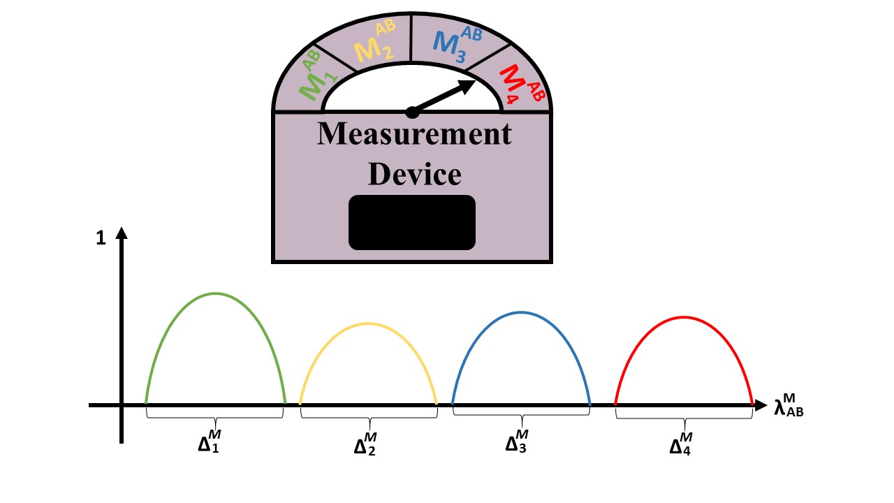
Although MOMF approaches symmetrically toward the preparation and measurement procedure, there is a conceptual difference between the forms of ΛPsuperscriptΛ𝑃\Lambda^{P} and ΛMsuperscriptΛ𝑀\Lambda^{M}. In principle, it is possible for different preparation methods to share some ontic states in their supports (this is the definition of ψ𝜓\psi-epistemic models). However, in the measurement ontic state space ΛMsuperscriptΛ𝑀\Lambda^{M}, this statement cannot hold, meaning that different regions of the ontic space (corresponding to different outcomes) are disjoint. Note that the outcomes of a measurement device correspond to different orthogonal POVM. Hence, from the operational points of view, the probability of being in an (operational) state which is compatible with two orthogonal POVMs is equal to zero. This operational claim can be confirmed by our daily experience, where we have never seen a measurement’s pointer being in two different outcomes at the same time. From the ontological points of view, one should note that ΛMsuperscriptΛ𝑀\Lambda^{M} must be composed of several non-overlapping regions, corresponding to several measurement outcomes. Otherwise, we could have a set of shared ontic states λMsuperscript𝜆𝑀\lambda^{M}, each of which being (ontologically) compatible with (operationally) incompatible states. Hence, via mirroring the observations coming from the operational level of QM into the ontological level, we have the following assumption. Figure (4) depicts this situation.

Assumption 3.1.

The ontic state space of a measurement device, ΛMsuperscriptΛ𝑀\Lambda^{M}, is composed of different non-overlapping regions, ΔiMsubscriptsuperscriptΔ𝑀𝑖\Delta^{M}_{i}, corresponding to its several outcomes. A measurement device with n𝑛n possible outcomes satisfies the following condition.

supp(λM)=Δ1M\sqcupdotΔ2M\sqcupdot\sqcupdotΔnM𝑠𝑢𝑝𝑝superscript𝜆𝑀subscriptsuperscriptΔ𝑀1\sqcupdotsubscriptsuperscriptΔ𝑀2\sqcupdot\sqcupdotsubscriptsuperscriptΔ𝑀𝑛supp(\lambda^{M})=\Delta^{M}_{1}\sqcupdot\Delta^{M}_{2}\sqcupdot...\sqcupdot\Delta^{M}_{n} (3.10)
Refer to caption
Figure 4: The ontic space of a measurement device is composed of several non-overlapping regions corresponding to its several outcomes. In this picture, the measurement device has four outcomes whose corresponding supports, ΔiMsubscriptsuperscriptΔ𝑀𝑖\Delta^{M}_{i}, are disjoint.
Proposition 3.2.

For systems A𝐴A and B𝐵B whose hypothetical composite system AB𝐴𝐵AB is (operationally) prepared and measured by PABsubscript𝑃𝐴𝐵P_{AB} and MABsuperscript𝑀𝐴𝐵M^{AB}, bipartite MOMF posits two ontic state spaces ΛABPsuperscriptsubscriptΛ𝐴𝐵𝑃\Lambda_{AB}^{P}, ΛABMsuperscriptsubscriptΛ𝐴𝐵𝑀\Lambda_{AB}^{M} and prescribes two probability distributions over them for every PABsubscript𝑃𝐴𝐵P_{AB} and MABsuperscript𝑀𝐴𝐵M^{AB}, denoted density functions pr(λABPPAB)𝑝𝑟conditionalsubscriptsuperscript𝜆𝑃𝐴𝐵subscript𝑃𝐴𝐵pr(\lambda^{P}_{AB}\mid P_{AB}) and pr(λABMMAB)𝑝𝑟conditionalsubscriptsuperscript𝜆𝑀𝐴𝐵superscript𝑀𝐴𝐵pr(\lambda^{M}_{AB}\mid M^{AB}) and a probability distribution over the different outcomes mABsuperscript𝑚𝐴𝐵m^{AB} of a measurement MABsuperscript𝑀𝐴𝐵M^{AB} for every pair of ontic states (λABP,λABM)ΛABP×ΛABMsubscriptsuperscript𝜆𝑃𝐴𝐵subscriptsuperscript𝜆𝑀𝐴𝐵subscriptsuperscriptΛ𝑃𝐴𝐵subscriptsuperscriptΛ𝑀𝐴𝐵(\lambda^{P}_{AB},\lambda^{M}_{AB})\in\Lambda^{P}_{AB}\times\Lambda^{M}_{AB}, denoted response function pr(mABλABP,λABM)𝑝𝑟conditionalsuperscript𝑚𝐴𝐵subscriptsuperscript𝜆𝑃𝐴𝐵subscriptsuperscript𝜆𝑀𝐴𝐵pr(m^{AB}\mid\lambda^{P}_{AB},\lambda^{M}_{AB}). Finally, for all PABsubscript𝑃𝐴𝐵P_{AB} and MABsuperscript𝑀𝐴𝐵M^{AB}, it must satisfy all the following conditions

ΛABPpr(λABPPAB)𝑑λABP=1subscriptsubscriptsuperscriptΛ𝑃𝐴𝐵𝑝𝑟conditionalsubscriptsuperscript𝜆𝑃𝐴𝐵subscript𝑃𝐴𝐵differential-dsubscriptsuperscript𝜆𝑃𝐴𝐵1\int_{\Lambda^{P}_{AB}}pr(\lambda^{P}_{AB}\mid P_{AB})d\lambda^{P}_{AB}=1 (3.11)
ΛABMpr(λABMMAB)𝑑λABM=1subscriptsubscriptsuperscriptΛ𝑀𝐴𝐵𝑝𝑟conditionalsubscriptsuperscript𝜆𝑀𝐴𝐵superscript𝑀𝐴𝐵differential-dsubscriptsuperscript𝜆𝑀𝐴𝐵1\int_{\Lambda^{M}_{AB}}pr(\lambda^{M}_{AB}\mid M^{AB})d\lambda^{M}_{AB}=1 (3.12)
mABpr(mABλABP,λABM)=1subscriptsuperscript𝑚𝐴𝐵𝑝𝑟conditionalsuperscript𝑚𝐴𝐵subscriptsuperscript𝜆𝑃𝐴𝐵subscriptsuperscript𝜆𝑀𝐴𝐵1\sum_{m^{AB}}pr(m^{AB}\mid\lambda^{P}_{AB},\lambda^{M}_{AB})=1 (3.13)
pr(mABPAB,MAB)=𝑝𝑟conditionalsuperscript𝑚𝐴𝐵subscript𝑃𝐴𝐵superscript𝑀𝐴𝐵absent\displaystyle pr(m^{AB}\mid P_{AB},M^{AB})= (3.14)
ΛABPΛABMdλABPdλABMpr(\displaystyle\int_{\Lambda^{P}_{AB}}\int_{\Lambda^{M}_{AB}}d\lambda^{P}_{AB}d\lambda^{M}_{AB}pr( λABPPAB)pr(λABMMAB)pr(mABλABP,λABM)\displaystyle\lambda^{P}_{AB}\mid P_{AB})pr(\lambda^{M}_{AB}\mid M^{AB})pr(m^{AB}\mid\lambda^{P}_{AB},\lambda^{M}_{AB})
Proof.

From 3.1, define a MOMF model for the enlarged system AB𝐴𝐵AB. Make the PM-Separability assumption (3.2) for AB𝐴𝐵AB. ∎

Definition 3.3.

Within MOMF, the Preparation Independence Postulate, PIP in MOMF, assumes the separability of the preparation ontic state space of the composite system AB𝐴𝐵AB, ΛABPsubscriptsuperscriptΛ𝑃𝐴𝐵\Lambda^{P}_{AB} in the following way.

ΛABP=ΛAP×ΛBPλABP=(λAP,λBP)subscriptsuperscriptΛ𝑃𝐴𝐵subscriptsuperscriptΛ𝑃𝐴subscriptsuperscriptΛ𝑃𝐵subscriptsuperscript𝜆𝑃𝐴𝐵subscriptsuperscript𝜆𝑃𝐴subscriptsuperscript𝜆𝑃𝐵\Lambda^{P}_{AB}=\Lambda^{P}_{A}\times\Lambda^{P}_{B}\equiv\lambda^{P}_{AB}=(\lambda^{P}_{A},\lambda^{P}_{B}) (3.15)
pr(λABPPAB)=pr(λAPPA)pr(λBPPB)𝑝𝑟conditionalsubscriptsuperscript𝜆𝑃𝐴𝐵subscript𝑃𝐴𝐵𝑝𝑟conditionalsubscriptsuperscript𝜆𝑃𝐴subscript𝑃𝐴𝑝𝑟conditionalsubscriptsuperscript𝜆𝑃𝐵subscript𝑃𝐵pr(\lambda^{P}_{AB}\mid P_{AB})=pr(\lambda^{P}_{A}\mid P_{A})pr(\lambda^{P}_{B}\mid P_{B}) (3.16)

3.2 The PBR Theorem in MOMF

Translating the details of the PBR’s operational scenario in MOMF, now, we can see the reason of why the PBR’s conclusion is not necessarily correct. First of all, let us explicitly express all the constraints on MOMF entailed by PBR’s scenario.

  1. 1.

    We assume that the PM𝑃𝑀PM separability assumption is valid,

    ΛPM=ΛP×ΛMλPM=(λP,λM)superscriptΛ𝑃𝑀superscriptΛ𝑃superscriptΛ𝑀superscript𝜆𝑃𝑀superscript𝜆𝑃superscript𝜆𝑀\Lambda^{PM}=\Lambda^{P}\times\Lambda^{M}\equiv\lambda^{PM}=(\lambda^{P},\lambda^{M}) (3.17)
    pr(λPMPM)=pr(λPP)pr(λMM)𝑝𝑟conditionalsuperscript𝜆𝑃𝑀𝑃𝑀𝑝𝑟conditionalsuperscript𝜆𝑃𝑃𝑝𝑟conditionalsuperscript𝜆𝑀𝑀pr(\lambda^{PM}\mid PM)=pr(\lambda^{P}\mid P)pr(\lambda^{M}\mid M) (3.18)
  2. 2.

    According to PBR’s scenario, the preparation procedures are operationally separable,

    PAB=(PA,PB)subscript𝑃𝐴𝐵subscript𝑃𝐴subscript𝑃𝐵P_{AB}=(P_{A},P_{B}) (3.19)
    ρAB=ρAρBsubscript𝜌𝐴𝐵tensor-productsubscript𝜌𝐴subscript𝜌𝐵\rho_{AB}=\rho_{A}\otimes\rho_{B} (3.20)
  3. 3.

    According to PBR’s scenario, the measurement procedures are entangled,

    MiAB(MiA,MiB)subscriptsuperscript𝑀𝐴𝐵𝑖subscriptsuperscript𝑀𝐴𝑖subscriptsuperscript𝑀𝐵𝑖M^{AB}_{i}\neq(M^{A}_{i},M^{B}_{i}) (3.21)

    .

  4. 4.

    We assume that the PIP assumption is valid,

    ΛABP=ΛAP×ΛBPλABP=(λAP,λBP)subscriptsuperscriptΛ𝑃𝐴𝐵subscriptsuperscriptΛ𝑃𝐴subscriptsuperscriptΛ𝑃𝐵subscriptsuperscript𝜆𝑃𝐴𝐵subscriptsuperscript𝜆𝑃𝐴subscriptsuperscript𝜆𝑃𝐵\Lambda^{P}_{AB}=\Lambda^{P}_{A}\times\Lambda^{P}_{B}\equiv\lambda^{P}_{AB}=(\lambda^{P}_{A},\lambda^{P}_{B}) (3.22)
    pr(λABPPAB)=pr(λAPPA)pr(λBPPB)𝑝𝑟conditionalsubscriptsuperscript𝜆𝑃𝐴𝐵subscript𝑃𝐴𝐵𝑝𝑟conditionalsubscriptsuperscript𝜆𝑃𝐴subscript𝑃𝐴𝑝𝑟conditionalsubscriptsuperscript𝜆𝑃𝐵subscript𝑃𝐵pr(\lambda^{P}_{AB}\mid P_{AB})=pr(\lambda^{P}_{A}\mid P_{A})pr(\lambda^{P}_{B}\mid P_{B}) (3.23)
  5. 5.

    Our model is ψ𝜓\psi-epistemic; Some (preparation) ontic states come from a common region which is compatible with all of the four possible preparation procedures,

    (λAP,λBP)ΔAP×ΔBPsubscriptsuperscript𝜆𝑃𝐴subscriptsuperscript𝜆𝑃𝐵subscriptsuperscriptΔ𝑃𝐴subscriptsuperscriptΔ𝑃𝐵(\lambda^{P}_{A},\lambda^{P}_{B})\in\Delta^{P}_{A}\times\Delta^{P}_{B} (3.24)
  6. 6.

    The support of the measurement ontic space ΛABMsubscriptsuperscriptΛ𝑀𝐴𝐵\Lambda^{M}_{AB} consists of four disjoint regions corresponding to four measurement outcomes,

    λABMΔABM=Δ1M\sqcupdotΔ2M\sqcupdotΔ3M\sqcupdotΔ4Msubscriptsuperscript𝜆𝑀𝐴𝐵subscriptsuperscriptΔ𝑀𝐴𝐵subscriptsuperscriptΔ𝑀1\sqcupdotsubscriptsuperscriptΔ𝑀2\sqcupdotsubscriptsuperscriptΔ𝑀3\sqcupdotsubscriptsuperscriptΔ𝑀4\lambda^{M}_{AB}\in\Delta^{M}_{AB}=\Delta^{M}_{1}\sqcupdot\Delta^{M}_{2}\sqcupdot\Delta^{M}_{3}\sqcupdot\Delta^{M}_{4} (3.25)
Remark 3.1.

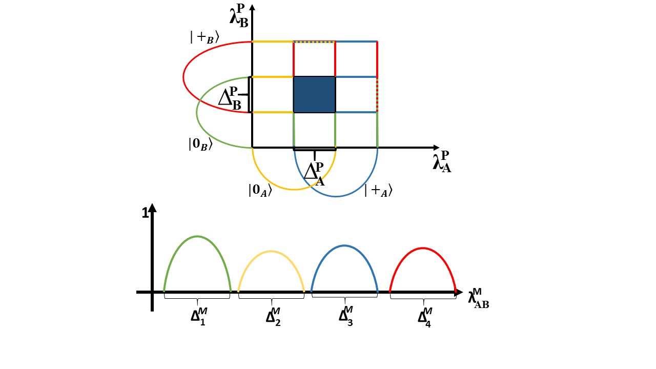
Figure (5) depicts the preparation and measurement ontic state spaces ΛABPsubscriptsuperscriptΛ𝑃𝐴𝐵\Lambda^{P}_{AB} and ΛABMsubscriptsuperscriptΛ𝑀𝐴𝐵\Lambda^{M}_{AB}, separately. As it was already explained, the overlap region ΔAP×ΔBPsubscriptsuperscriptΔ𝑃𝐴subscriptsuperscriptΔ𝑃𝐵\Delta^{P}_{A}\times\Delta^{P}_{B} is a problematic region for ψ𝜓\psi-epistemic OMF models. A three-dimensional representation of this problematic region is provided in figure (6). In what follows, we are going to prove that ψ𝜓\psi-epistemic models can reproduce PBR statistics without any contradiction if the ontic states of the measurement device become involved.
Refer to caption
Figure 5: The preparation and measurement ontic state spaces ΛABPsubscriptsuperscriptΛ𝑃𝐴𝐵\Lambda^{P}_{AB} and ΛABMsubscriptsuperscriptΛ𝑀𝐴𝐵\Lambda^{M}_{AB} for the PBR’s scenario. The upper graph represents the preparation ontic space, ΛABPsubscriptsuperscriptΛ𝑃𝐴𝐵\Lambda^{P}_{AB}, which is assumed to be the Cartesian product of ΛAPsubscriptsuperscriptΛ𝑃𝐴\Lambda^{P}_{A} and ΛBPsubscriptsuperscriptΛ𝑃𝐵\Lambda^{P}_{B}. The lower picture shows the measurement ontic state ΛABMsubscriptsuperscriptΛ𝑀𝐴𝐵\Lambda^{M}_{AB}. This space is not separable into ΛAMsubscriptsuperscriptΛ𝑀𝐴\Lambda^{M}_{A} and ΛBMsubscriptsuperscriptΛ𝑀𝐵\Lambda^{M}_{B}.

Step 1. In this step, by combing the above constraints on MOMF definition, we derive further required equations.

Making the PIP and the PM separability assumptions, the total ontic state space ΛABPMsubscriptsuperscriptΛ𝑃𝑀𝐴𝐵\Lambda^{PM}_{AB} can be obtained as follows,

ΛABPM=ΛABP×ΛABM=ΛAP×ΛBP×ΛABMsubscriptsuperscriptΛ𝑃𝑀𝐴𝐵subscriptsuperscriptΛ𝑃𝐴𝐵subscriptsuperscriptΛ𝑀𝐴𝐵subscriptsuperscriptΛ𝑃𝐴subscriptsuperscriptΛ𝑃𝐵subscriptsuperscriptΛ𝑀𝐴𝐵\Lambda^{PM}_{AB}=\Lambda^{P}_{AB}\times\Lambda^{M}_{AB}=\Lambda^{P}_{A}\times\Lambda^{P}_{B}\times\Lambda^{M}_{AB} (3.26)

Exactly similar to (2.12), the support of the preparation ontic state, supp(λABP)𝑠𝑢𝑝𝑝subscriptsuperscript𝜆𝑃𝐴𝐵supp(\lambda^{P}_{AB}), is composed nine mutually exclusive sub-regions.

supp(λABPPAB)=R11P\sqcupdotR12P\sqcupdot\sqcupdotR33P𝑠𝑢𝑝𝑝conditionalsubscriptsuperscript𝜆𝑃𝐴𝐵subscript𝑃𝐴𝐵subscriptsuperscript𝑅𝑃11\sqcupdotsubscriptsuperscript𝑅𝑃12\sqcupdot\sqcupdotsubscriptsuperscript𝑅𝑃33supp(\lambda^{P}_{AB}\mid P_{AB})=R^{P}_{11}\sqcupdot R^{P}_{12}\sqcupdot...\sqcupdot R^{P}_{33} (3.27)

On the other hand, the support of the measurement ontic state, supp(λABMsupp(\lambda^{M}_{AB}, is composed of four mutually exclusive sub-regions. Placing (3.25) in (3.26), it can be understood that the support of the total ontic state, supp(λABPMsupp(\lambda^{PM}_{AB}, is composed of thirty-six mutually exclusive sub-regions.

supp(λABPMPAB,MAB)=supp(λABPPAB)×supp(λABMMAB)=𝑠𝑢𝑝𝑝conditionalsubscriptsuperscript𝜆𝑃𝑀𝐴𝐵subscript𝑃𝐴𝐵superscript𝑀𝐴𝐵𝑠𝑢𝑝𝑝conditionalsubscriptsuperscript𝜆𝑃𝐴𝐵subscript𝑃𝐴𝐵𝑠𝑢𝑝𝑝conditionalsubscriptsuperscript𝜆𝑀𝐴𝐵superscript𝑀𝐴𝐵absentsupp(\lambda^{PM}_{AB}\mid P_{AB},M^{AB})=supp(\lambda^{P}_{AB}\mid P_{AB})\times supp(\lambda^{M}_{AB}\mid M^{AB})= (3.28)
(R11P\sqcupdot\sqcupdotR33P)×(Δ1M\sqcupdot\sqcupdotΔ4M)subscriptsuperscript𝑅𝑃11\sqcupdot\sqcupdotsubscriptsuperscript𝑅𝑃33subscriptsuperscriptΔ𝑀1\sqcupdot\sqcupdotsubscriptsuperscriptΔ𝑀4(R^{P}_{11}\sqcupdot...\sqcupdot R^{P}_{33})\times(\Delta^{M}_{1}\sqcupdot...\sqcupdot\Delta^{M}_{4})

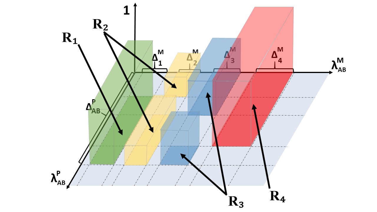
We have already seen that the problem of the ψ𝜓\psi-epistemic models is the existence of the overlap region R22Psubscriptsuperscript𝑅𝑃22R^{P}_{22}, and not the other regions. Hence, to assess the ability of a ψ𝜓\psi-epistemic MOMF model in reproducing PBR statistics, it suffices to check this ability for the states belonging to this problematic region, λABPMR22P×ΔABMsubscriptsuperscript𝜆𝑃𝑀𝐴𝐵subscriptsuperscript𝑅𝑃22subscriptsuperscriptΔ𝑀𝐴𝐵\lambda^{PM}_{AB}\in R^{P}_{22}\times\Delta^{M}_{AB}. In the total ontic state space ΛABPMsubscriptsuperscriptΛ𝑃𝑀𝐴𝐵\Lambda^{PM}_{AB}, there are four sub-regions being compatible with R22P=ΔAP×ΔAPsubscriptsuperscript𝑅𝑃22subscriptsuperscriptΔ𝑃𝐴subscriptsuperscriptΔ𝑃𝐴R^{P}_{22}=\Delta^{P}_{A}\times\Delta^{P}_{A}. Let us denote them by R1subscript𝑅1R_{1}, R2subscript𝑅2R_{2}, R3subscript𝑅3R_{3} and R4subscript𝑅4R_{4}, where Ri=R22P×ΔiMsubscript𝑅𝑖subscriptsuperscript𝑅𝑃22subscriptsuperscriptΔ𝑀𝑖R_{i}=R^{P}_{22}\times\Delta^{M}_{i}.

Figure (6) provides a three dimensional representation of these regions. Note that these regions are disjoint, and their union constructs the problematic region R22P×ΔABMsubscriptsuperscript𝑅𝑃22subscriptsuperscriptΔ𝑀𝐴𝐵R^{P}_{22}\times\Delta^{M}_{AB},

ΔAP×ΔBP×ΔABM=R1\sqcupdotR2\sqcupdotR3\sqcupdotR4subscriptsuperscriptΔ𝑃𝐴subscriptsuperscriptΔ𝑃𝐵subscriptsuperscriptΔ𝑀𝐴𝐵subscript𝑅1\sqcupdotsubscript𝑅2\sqcupdotsubscript𝑅3\sqcupdotsubscript𝑅4\Delta^{P}_{A}\times\Delta^{P}_{B}\times\Delta^{M}_{AB}=R_{1}\sqcupdot R_{2}\sqcupdot R_{3}\sqcupdot R_{4} (3.29)

Finally, we have the following equation for computing the probability of finding different outcomes.

pr(mABPAB,MAB)=𝑝𝑟conditionalsuperscript𝑚𝐴𝐵subscript𝑃𝐴𝐵superscript𝑀𝐴𝐵absentpr(m^{AB}\mid P_{AB},M^{AB})= (3.30)

ΛAPΛBPΛABM𝑑λAP𝑑λBP𝑑λABMpr(λAPPA)pr(λBPPB)pr(λABMMAB)pr(mABλAP,λBP,λABM)subscriptsubscriptsuperscriptΛ𝑃𝐴subscriptsubscriptsuperscriptΛ𝑃𝐵subscriptsubscriptsuperscriptΛ𝑀𝐴𝐵differential-dsubscriptsuperscript𝜆𝑃𝐴differential-dsubscriptsuperscript𝜆𝑃𝐵differential-dsubscriptsuperscript𝜆𝑀𝐴𝐵𝑝𝑟conditionalsubscriptsuperscript𝜆𝑃𝐴subscript𝑃𝐴𝑝𝑟conditionalsubscriptsuperscript𝜆𝑃𝐵subscript𝑃𝐵𝑝𝑟conditionalsubscriptsuperscript𝜆𝑀𝐴𝐵superscript𝑀𝐴𝐵𝑝𝑟conditionalsuperscript𝑚𝐴𝐵subscriptsuperscript𝜆𝑃𝐴subscriptsuperscript𝜆𝑃𝐵subscriptsuperscript𝜆𝑀𝐴𝐵\int_{\Lambda^{P}_{A}}\int_{\Lambda^{P}_{B}}\int_{\Lambda^{M}_{AB}}d\lambda^{P}_{A}d\lambda^{P}_{B}d\lambda^{M}_{AB}pr(\lambda^{P}_{A}\mid P_{A})pr(\lambda^{P}_{B}\mid P_{B})pr(\lambda^{M}_{AB}\mid M^{AB})pr(m^{AB}\mid\lambda^{P}_{A},\lambda^{P}_{B},\lambda^{M}_{AB})

Step 2. In this step, PBR’s observations will be expressed within MOMF.

Observation 1: Our measurement device can select the outcomes which are non orthogonal to the prepared state. So the probability of choosing an outcome which is orthogonal to the prepared state is zero. This observation leads to the four following equations on the operational level,

operational level{pr(mAB=1ψAB=|0A0B,MAB)=Tr(M1ABρAB1)=0pr(mAB=2ψAB=|0A+B,MAB)=Tr(M2ABρAB2)=0pr(mAB=3ψAB=|+A0B,MAB)=Tr(M3ABρAB3)=0pr(mAB=4ψAB=|+A+B,MAB)=Tr(M4ABρAB4)=0\textup{operational level}\begin{cases}pr(m^{AB}=1\mid\psi_{AB}=\ket{0_{A}0_{B}},M^{AB})=Tr(M^{AB}_{1}\rho^{1}_{AB})=0\\ pr(m^{AB}=2\mid\psi_{AB}=\ket{0_{A}+_{B}},M^{AB})=Tr(M^{AB}_{2}\rho^{2}_{AB})=0\\ pr(m^{AB}=3\mid\psi_{AB}=\ket{+_{A}0_{B}},M^{AB})=Tr(M^{AB}_{3}\rho^{3}_{AB})=0\\ pr(m^{AB}=4\mid\psi_{AB}=\ket{+_{A}+_{B}},M^{AB})=Tr(M^{AB}_{4}\rho^{4}_{AB})=0\\ \end{cases} (3.31)

Combining the above results with equations (3.28) and (3.30), one can convert this set of four operational equations into the following set of equations at the ontic (MOMF) level of QM.

ontic level{pr(mAB=1λAP,λBP,λABM)=0whenλABPM(R21P\sqcupdotR22P\sqcupdotR31P\sqcupdotR32P)×(Δ1M)pr(mAB=2λAP,λBP,λABM)=0whenλABPM(R11P\sqcupdotR12P\sqcupdotR21P\sqcupdotR22P)×(Δ2M)pr(mAB=3λAP,λBP,λABM)=0whenλABPM(R22P\sqcupdotR23P\sqcupdotR32P\sqcupdotR33P)×(Δ3M)pr(mAB=4λAP,λBP,λABM)=0whenλABPM(R12P\sqcupdotR23P\sqcupdotR22P\sqcupdotR23P)×(Δ4M)ontic levelcases𝑝𝑟superscript𝑚𝐴𝐵conditional1subscriptsuperscript𝜆𝑃𝐴subscriptsuperscript𝜆𝑃𝐵subscriptsuperscript𝜆𝑀𝐴𝐵0𝑤𝑒𝑛subscriptsuperscript𝜆𝑃𝑀𝐴𝐵subscriptsuperscript𝑅𝑃21\sqcupdotsubscriptsuperscript𝑅𝑃22\sqcupdotsubscriptsuperscript𝑅𝑃31\sqcupdotsubscriptsuperscript𝑅𝑃32subscriptsuperscriptΔ𝑀1otherwise𝑝𝑟superscript𝑚𝐴𝐵conditional2subscriptsuperscript𝜆𝑃𝐴subscriptsuperscript𝜆𝑃𝐵subscriptsuperscript𝜆𝑀𝐴𝐵0𝑤𝑒𝑛subscriptsuperscript𝜆𝑃𝑀𝐴𝐵subscriptsuperscript𝑅𝑃11\sqcupdotsubscriptsuperscript𝑅𝑃12\sqcupdotsubscriptsuperscript𝑅𝑃21\sqcupdotsubscriptsuperscript𝑅𝑃22subscriptsuperscriptΔ𝑀2otherwise𝑝𝑟superscript𝑚𝐴𝐵conditional3subscriptsuperscript𝜆𝑃𝐴subscriptsuperscript𝜆𝑃𝐵subscriptsuperscript𝜆𝑀𝐴𝐵0𝑤𝑒𝑛subscriptsuperscript𝜆𝑃𝑀𝐴𝐵subscriptsuperscript𝑅𝑃22\sqcupdotsubscriptsuperscript𝑅𝑃23\sqcupdotsubscriptsuperscript𝑅𝑃32\sqcupdotsubscriptsuperscript𝑅𝑃33subscriptsuperscriptΔ𝑀3otherwise𝑝𝑟superscript𝑚𝐴𝐵conditional4subscriptsuperscript𝜆𝑃𝐴subscriptsuperscript𝜆𝑃𝐵subscriptsuperscript𝜆𝑀𝐴𝐵0𝑤𝑒𝑛subscriptsuperscript𝜆𝑃𝑀𝐴𝐵subscriptsuperscript𝑅𝑃12\sqcupdotsubscriptsuperscript𝑅𝑃23\sqcupdotsubscriptsuperscript𝑅𝑃22\sqcupdotsubscriptsuperscript𝑅𝑃23subscriptsuperscriptΔ𝑀4otherwise\textup{ontic level}\begin{cases}pr(m^{AB}=1\mid\lambda^{P}_{A},\lambda^{P}_{B},\lambda^{M}_{AB})=0\hskip 5.69054ptwhen\hskip 5.69054pt\lambda^{PM}_{AB}\in(R^{P}_{21}\sqcupdot{\color[rgb]{1,0,0}\definecolor[named]{pgfstrokecolor}{rgb}{1,0,0}R^{P}_{22}}\sqcupdot R^{P}_{31}\sqcupdot R^{P}_{32})\times(\Delta^{M}_{1})\\ pr(m^{AB}=2\mid\lambda^{P}_{A},\lambda^{P}_{B},\lambda^{M}_{AB})=0\hskip 5.69054ptwhen\hskip 5.69054pt\lambda^{PM}_{AB}\in(R^{P}_{11}\sqcupdot R^{P}_{12}\sqcupdot R^{P}_{21}\sqcupdot{\color[rgb]{1,0,0}\definecolor[named]{pgfstrokecolor}{rgb}{1,0,0}R^{P}_{22}})\times(\Delta^{M}_{2})\\ pr(m^{AB}=3\mid\lambda^{P}_{A},\lambda^{P}_{B},\lambda^{M}_{AB})=0\hskip 5.69054ptwhen\hskip 5.69054pt\lambda^{PM}_{AB}\in({\color[rgb]{1,0,0}\definecolor[named]{pgfstrokecolor}{rgb}{1,0,0}R^{P}_{22}}\sqcupdot R^{P}_{23}\sqcupdot R^{P}_{32}\sqcupdot R^{P}_{33})\times(\Delta^{M}_{3})\\ pr(m^{AB}=4\mid\lambda^{P}_{A},\lambda^{P}_{B},\lambda^{M}_{AB})=0\hskip 5.69054ptwhen\hskip 5.69054pt\lambda^{PM}_{AB}\in(R^{P}_{12}\sqcupdot R^{P}_{23}\sqcupdot{\color[rgb]{1,0,0}\definecolor[named]{pgfstrokecolor}{rgb}{1,0,0}R^{P}_{22}}\sqcupdot R^{P}_{23})\times(\Delta^{M}_{4})\\ \end{cases} (3.32)

Observation 2: According to equation (3.13), regardless of which quantum state has been prepared, the sum of the response functions must be equal to one.

Σi=14pr(mAB=iλAP,λBP,λABM)subscriptsuperscriptΣ4𝑖1𝑝𝑟superscript𝑚𝐴𝐵conditional𝑖subscriptsuperscript𝜆𝑃𝐴subscriptsuperscript𝜆𝑃𝐵subscriptsuperscript𝜆𝑀𝐴𝐵\Sigma^{4}_{i=1}pr(m^{AB}=i\mid\lambda^{P}_{A},\lambda^{P}_{B},\lambda^{M}_{AB}) (3.33)
Refer to caption
Figure 6: An illustration of a specific sub-region of the total ontic state space for PBR’s scenario, namely ΔAP×ΔBP×ΛABMsubscriptsuperscriptΔ𝑃𝐴subscriptsuperscriptΔ𝑃𝐵subscriptsuperscriptΛ𝑀𝐴𝐵\Delta^{P}_{A}\times\Delta^{P}_{B}\times\Lambda^{M}_{AB}. This 3D-representation has been obtained from the Cartesian product of the previous 2D-representations of the preparation and measurement procedures in figures (3) and (4). Clearly, this sub-region is composed of four disjoint parts, each of which being able to reproduce PBR’s statistics without any contradiction.

Step 3. Fortunately, there is no contradiction between the implications of the first observation, in (3.32), and the consequences of the second observation, in (3.33):

The ontic states λABPM=(λAP,λBP,λABM)subscriptsuperscript𝜆𝑃𝑀𝐴𝐵subscriptsuperscript𝜆𝑃𝐴subscriptsuperscript𝜆𝑃𝐵subscriptsuperscript𝜆𝑀𝐴𝐵\lambda^{PM}_{AB}=(\lambda^{P}_{A},\lambda^{P}_{B},\lambda^{M}_{AB}) in equations of the set (3.32) are not the same. Rather, each triplet belongs to one specific sub-region of the total ontic space which is disjoint from the others. Hence, if the response function of our model assigns zero to one triplet, the other three triplets become non-zero. And exactly these three triplets can reproduce the first observation (3.32). To be precise, different parts of the measurement ontic state space are completely disjoint from each other. So, we have

|ΔiMΔjiM|=0subscriptsuperscriptΔ𝑀𝑖subscriptsuperscriptΔ𝑀𝑗𝑖0|\Delta^{M}_{i}\cap\Delta^{M}_{j\neq i}|=0 (3.34)

Hence, supports of the ontic state in four equations (3.32) do not share any common ontic state,

|(R22P×ΔiM)(R22P×ΔjiM)|=0subscriptsuperscript𝑅𝑃22subscriptsuperscriptΔ𝑀𝑖subscriptsuperscript𝑅𝑃22subscriptsuperscriptΔ𝑀𝑗𝑖0|({\color[rgb]{1,0,0}\definecolor[named]{pgfstrokecolor}{rgb}{1,0,0}R^{P}_{22}}\times\Delta^{M}_{i})\cap({\color[rgb]{1,0,0}\definecolor[named]{pgfstrokecolor}{rgb}{1,0,0}R^{P}_{22}}\times\Delta^{M}_{j\neq i})|=0 (3.35)

4 Conclusion

First, I investigated the PBR theorem and its underlying framework, OMF. Pointing to a problem inside the OMF definition, I defined a modified version of OMF, MOMF. Translating the PBR’s scenario in MOMF, I showed that PBR’s claim in rejecting the epistemic view is not because of the nature of the wavefunction. Rather, (I argued that) the reason of why PBR have found such a result lies in the OMF definition. That this, the PBR theorem has vanished within MOMF. Inserting the measurement ontic state was the key idea of this paper. This analysis suggests that the importance of PBR’s work is not because of their conclusion about the nature of the wavefunction. Rather, PBR’s finding reveals a significant deficiency of OMF in not considering the ontic level of measurement devices. It is important to note that, the arguments of this paper do not lead to any conclusion about the nature of wavefunction. However, the paper reveals that PBR’s arguments cannot reject the epistemic view of the wavefunction.

Acknowledgements

Special thanks to Erik Curiel and Neil Dewar for their very careful reviews and comments. Also, I would like to thank Stephan Hartmann, Detlef Dürr, Ward Struyve and Michael Cuffaro for helpful feedback on an earlier draft. The author is supported by the MCMP.

References

  • [1] Nicholas Harrigan and Robert W Spekkens. Einstein, incompleteness, and the epistemic view of quantum states. Foundations of Physics, 40(2):125–157, 2010.
  • [2] Matt Leifer. Can the quantum state be interpreted statistically? Web log post.¡ http://mattleifer. info/2011/11/20/can-the-quantum-state-be-interpretedstatistically, 2011.
  • [3] Matthew Saul Leifer. Is the quantum state real? An extended review of ψ𝜓\psi-ontology theorems. arXiv preprint arXiv:1409.1570, 2014.
  • [4] Matthew F Pusey, Jonathan Barrett, and Terry Rudolph. On the reality of the quantum state. Nature Physics, 8(6):475–478, 2012.
  • [5] Maximilian Schlosshauer and Arthur Fine. No-go theorem for the composition of quantum systems. Physical review letters, 112(7):70407, 2014.
  • [6] Arijit Dutta, Marcin Pawłowski, and Marek Żukowski. Detection-efficiency loophole and the Pusey-Barrett-Rudolph theorem. Physical Review A, 91(4):042125, 2015.
  • [7] Michael JW Hall. Generalisations of the recent Pusey-Barrett-Rudolph theorem for statistical models of quantum phenomena. arXiv preprint arXiv:1111.6304, 2011.
  • [8] Joseph Emerson, Dmitry Serbin, Chris Sutherland, and Victor Veitch. The whole is greater than the sum of the parts: on the possibility of purely statistical interpretations of quantum theory. arXiv preprint arXiv:1312.1345, 2013.
  • [9] Andre O Ranchin. Progress in quantum foundations. PhD thesis, Citeseer, 2012.