How fast can one overcome the paradox of the energy transition? A physico-economic model for the European power grid

Abstract

The paradox of the energy transition is that the low marginal costs of new renewable energy sources (RES) drag electricity prices down and discourage investments in flexible productions that are needed to compensate for the lack of dispatchability of the new RES. The energy transition thus discourages the investments that are required for its own harmonious expansion. To investigate how this paradox can be overcome, we argue that, under certain assumptions, future electricity prices are rather accurately modeled from the residual load obtained by subtracting non-flexible productions from the load. Armed with the resulting economic indicator, we investigate future revenues for European power plants with various degree of flexibility. We find that, if neither carbon taxes nor fuel prices change, flexible productions would be financially rewarded better and sooner if the energy transition proceeds faster but at more or less constant total production, i.e. by reducing the production of thermal power plants at the same rate as the RES production increases. Less flexible productions, on the other hand, would see their revenue grow more moderately. Our results indicate that a faster energy transition with a quicker withdrawal of thermal power plants would reward flexible productions faster.

1 Introduction

1.1 The paradox of the energy transition

The goal of the energy transition is to meet energy demand from human activities in a sustainable way. In the electricity sector, the transition currently increases the penetration of productions from new renewable energy sources (RES), in particular solar photovoltaic panels (PV) and wind turbines (WT). These RES differ from the traditional productions they substitute for, in at least two very significant ways. First, they lack dispatchability and have little mechanical inertia, second, they have very low marginal production costs. Their lack of dispatchability and mechanical inertia requires additional flexible productions and possibly electrical energy storage (EES) to ensure the stability of the power grid as well as the balance of demand and supply at all times. Therefore increasing penetrations of new RES should be accompanied by significant investments in new facilities with rather long payback periods. However, the new RES’s low marginal cost brings spot electricity prices and thus beneficiary margins of electric power companies down, while further extending the payback period for investments in new facilities. The energy transition is therefore confronted with the paradox that it creates economic conditions which, at least temporarily, strongly discourage the infrastructural investments it needs to progress further. Because of that, a number of hydroelectric plant projects are currently frozen in Europe. To plan the next steps in the energy transition, to evaluate and anticipate the investments needed for its safe, steady progress, it is therefore important to get a relatively good quantitative estimate of future electricity prices. The key issue is whether production flexibility will soon be rewarded well enough that it will motivate investments in fast dispatchable power plants and EES at a level consistent with the rate at which RES penetration increases.

The traditional way to address such questions is to construct economic models for electricity production and consumption. Those models are standardly based on a number of assumptions on general economic conditions, demographic evolution, costs of different fuels, maintenance and production costs, amount of taxes and subsidies on energy production and so forth. Once all these ingredients are fixed, both the electricity demand and the marginal cost of different productions can be estimated, which determine the market price of electricity, from which one finally computes expected future revenues. From these revenues, investment decisions can ultimately be made. The accuracy of this procedure relies on the accuracy of each of the assumptions on which it is based. Unfortunately, the latter are to a high degree arbitrary – economic growth rates, unemployment rates (indicative of the volume of industrial activities), taxation amounts, fuel costs (in particular natural gas prices), carbon taxes and so forth cannot be predicted accurately on time scales of decades, corresponding to typical payback times for investments in the energy sector. In this manuscript we take a deliberately different approach, using as few working hypotheses as possible. Eurotranselec, our model to be presented below, is mostly based on physical conditions extracted from the size and production types of national power plant fleets as well as the electricity demand. We argue that it introduces a reliable though quite simple procedure to evaluate future electricity prices in the not too far future, given scenarios for the energy transition and the resulting evolution of power plant fleets. We use it to investigate revenues of electric power plants in a time window until 2020.

Figure 1: German residual load (green) and day-ahead electricity price (blue) for a winter (top) and summer (bottom) week in 2015 [data taken from ENTSO-E (2015a)]. Vertical dashed lines indicate noon time.

1.2 The residual load and electricity prices

Our starting observation is that electricity prices reflect the law of supply and demand. Accordingly they exhibit some degree of correlation with what flexible sources must generate to sustain load – the larger the difference between demand and non-dispatchable supply, the higher the electricity price. As a matter of fact, spot market prices are usually higher at times of larger imbalance between demand and non-dispatchable supply, when the imbalance leans strongly on the demand side. The corresponding missing amount of power is quantified by the residual load, which is defined as the difference between consumption and the sum of all non-flexible productions. With the residual load, the new RES are accounted for on the demand side and not as a production - they are seen as reducing the demand for the rest of the market. This is justified by their almost vanishing marginal production cost.

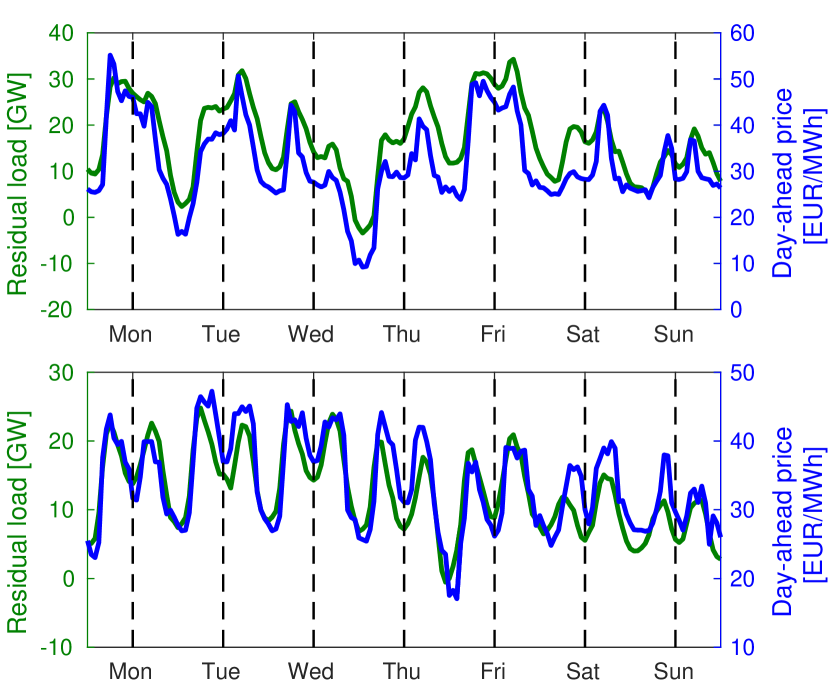
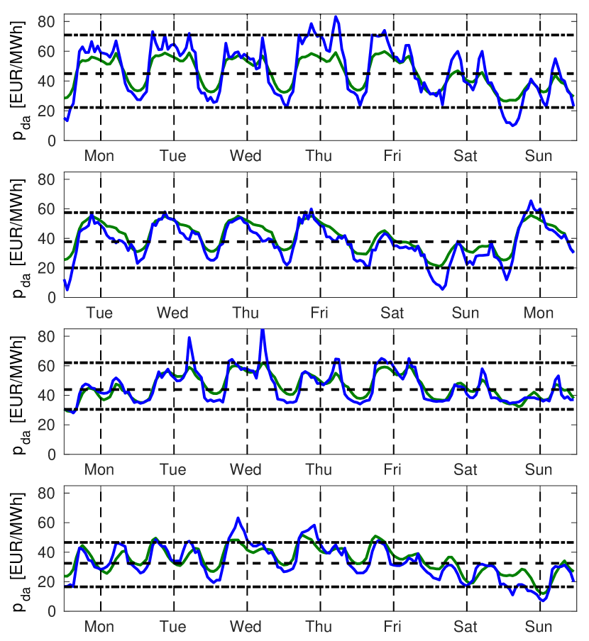
While some degree of correlation between the residual load and spot market prices is expected, a strong correlation between them has been reported by von Roon and Huber (2010) for the special case of Germany in 2007–2009, with a coefficient of determination $R^{2}\in[0.5,0.77]$. Fig. 1 confirms that a high degree of correlation between residual load and day-ahead market price prevails in Germany in 2015, which is quantified by a high value of Pearson’s correlation coefficient [see Eq. (4.1) below] $r=0.89$. Below we investigate the correlation between day-ahead prices and residual load further, for different European countries. We find that it always corresponds to a large, positive correlation coefficient, $r>0.5$, and furthermore that $r$ is generally higher in countries with larger penetration of RES (this is shown in Fig. 3 and will be discussed below). The energy transition will keep increasing the penetration of RES, it is therefore reasonable to expect that $r$ will increase in the future. If this is confirmed, the residual load will reflect the day-ahead price better and better. Day-ahead transactions represent a significant percentage of all electricity transactions (see Table 1 below), and their share of the total load is expected to increase with the end of long-term contracts in the liberalized European electricity market. Putting all this together, we propose to introduce a synthetic electricity price $p_{\mathrm{da}}(t)$ as a two-parameter, linear regression of the day-ahead price based on the residual load $R(t)$,

$$p_{\mathrm{da}}(t)=\Delta p_{\mathrm{da}}\,R(t)+p_{\mathrm{da}0}\,.$$ (1.1)

In this manuscript, the two parameters $\Delta p_{\mathrm{da}}$ and $p_{\mathrm{da}0}$ are determined country by country from a least square fit of 2015 day-ahead data with Eq (1.1). They are assumed to remain constant in the future, because we consider a relatively small time window, until 2020. However different scenarios can be considered, where $\Delta p_{\mathrm{da}}$ and $p_{\mathrm{da}0}$ evolve in time, for instance because economic conditions (fuel prices, subsidies and taxes) vary. Below we discuss in particular how $\Delta p_{\mathrm{da}}$ and $p_{\mathrm{da}0}$ qualitatively vary with varying carbon taxes and natural gas prices.

We think that $p_{\mathrm{da}}(t)$ is a reliable day-ahead electricity price because it reproduces qualitatively and even almost always quantitatively historical time series for the true spot market day-ahead price of electricity in all European countries we focus on. Not caught by our approach are extreme events, for instance corresponding to record low (high) RES productions with simultaneous record high (low) demand, giving unusually high price maxima (unusually low price minima).

Armed with $p_{\mathrm{da}}(t)$ we finally investigate the parallel evolution of the energy transition and the electricity prices in Germany and Spain and compute expected future revenues for various types of power plants, focusing on pumped-storage and conventional dam hydroelectric plants. Under our assumptions, that neither consumption, nor gas prices will change significantly in the foreseeable future, our investigations indicate that revenues will bounce back faster and higher if RES production increases faster and if this transition is accompanied by a simultaneous phasing-out of superfluous thermal productions.

1.3 Literature review

Studies of the impact of increased penetration of new RES on electricity prices abound. Many of them investigated historical data vs. the penetration of new RES to empirically express electricity prices as a function of green in-feed (Clò et al., 2015; Paraschiv et al., 2014). In the liberalized European market, electricity prices are determined by a merit order supply curve where production capacities are ordered according to their marginal costs. The effect of such merit order on historical electricity prices under increased penetration of new RES has been investigated by Cludius et al. (2014), who extrapolated their findings to evaluate future revenues of PV and WT. Going further, a number of studies investigated electricity markets where prices are determined by simulated merit orders with marginal costs as inputs (Sensfuss et al., 2008; Haas et al., 2013; Auer and Haas, 2016), which often rely on self-consistent optimizations. As interesting as these works are, they are based on heavy algorithms as well as many assumptions (for instance future fuel prices) to build the merit order. Schlachtberger et al. (2016) find that more flexible production is required as the penetration of new RES increases and that flexible sources become essential when the penetration of new RES reaches 50%.

By definition, the residual load gives indications on periods of surplus or deficit of production of new RES. Accordingly, it has been the focus of many recent investigations evaluating the needed capacity of EES, of thermal storage and of additional dispatchable productions to help absorb large penetrations of new RES (Schill, 2014; Saarinen et al., 2015; Ueckerdt et al., 2015; Schweiger et al., 2017). In his analysis of negative price regimes, Nicolosi (2012) illustrated a connection between the residual load and the merit order. To the best of our knowledge, von Roon and Huber (2010) have been the only ones so far to report a direct correlation between residual load and spot electricity prices. Their investigation of the German electricity market before 2010 further assumed that the coal and natural gas price determine the electricity price most of the time, because the German load back then required coal and gas power plants to produce most of the time. They therefore proposed to model electricity prices as a function of the natural gas price and of the residual load. Given uncertainties in future gas prices (as well as those of other fossil fuels) and the level of CO₂ taxes, we depart from that analysis and go one step further by modeling prices using the residual load only.

1.4 Our contribution

In this manuscript we construct a model to investigate future economic conditions in the European electricity sector. To construct our pricing algorithm, we depart from von Roon and Huber (2010) in that (i) we model electricity prices only as a function of the residual load, (ii) we take changes in production fleet and other scenarios into account in our study, (iii) we apply our study to most European countries, as they also exhibit high degrees of correlation between day-ahead prices and residual load, and (iv) our pricing procedure may be incorporated into an aggregated European grid (Pagnier and Jacquod, 2017). We call the resulting model Eurotranselec. In the period 2010–2015, after the work of von Roon and Huber (2010), the new RES penetration in Germany has dramatically increased, with the WT production more than doubling and the PV production more than tripling. Point (i) is therefore an important and necessary departure from von Roon and Huber (2010), because with this strong increase in new RES capacities, electricity prices are less often directly determined by natural gas prices. In analyzing other European countries, we moreover observe that the correlation between residual load and day-ahead prices is generally stronger in countries with higher penetration of RES. Because RES is expected to significantly increase in the future, it is natural to expect that this correlation will also increase. Additionally, day-ahead markets make a significant part of the total traded electrical energy (see Table 1 below), a share which will increase with the end of long-term contracts in the liberalized European market. It seems therefore reasonable to expect that the pricing model we present in this article will become more and more accurate as the energy transition proceeds. While von Roon and Huber (2010) should get the credit for uncovering an important correlation between residual load and spot market prices, the present manuscript uses the full analytical power behind this correlation for the first time, to the best of our knowledge. Our results allow to anticipate how the energy transition should proceed in its next steps in order to overcome the paradox described above.

The European electricity market is expected to evolve fast with the energy transition. New incentives and taxes may appear, different financial products related to electricity may be introduced, gas and other fuel prices may fluctuate. All this will modify the way electricity is both produced and consumed, and will significantly impact power plant revenues. Our purpose in this manuscript is however to investigate the relatively near future and see how financial conditions in the electricity sector will evolve in the next few years. Accordingly, our investigations deliberately assume a European electricity market where the penetration of RES increases and thermal power plants are withdrawn, all other things remaining constant. We stress that, to extrapolate our investigations to longer time scales, our approach needs to be revisited, for instance by considering different scenarios and pricing parameters $\Delta p_{\mathrm{da}}$ and $p_{\mathrm{da}0}$, or different consumption profiles. In A, we comment on how consumption profiles modified by active demand response could be incorporated in our model.

This manuscript is organized as follows. Section 2 defines the residual load. In Section 3 we comment briefly on electricity trading. In Section 4 we show the strong correlation between residual loads and day-ahead electricity prices in European countries and show that they are stronger in countries with more new RES. In Section 5 we construct a synthetic electricity price in each country considered in our model. That price is based on residual load and in Section 6 we use it to investigate future revenues of various types of electricity productions. We focus on conventional dam hydroelectricity, as it is one of the most flexible, more easily dispatchable electricity production and on pumped-hydro, which is to date the dominant EES solution for which a number of projects are however currently put on hold in Europe because of low electricity prices. We finally discuss other productions, depending on their number of operation hours per year. Conclusions and future perspectives are given in Section 7.

2 Residual load and must-run

The residual load is defined as the difference between the total consumption and the sum of all non-flexible productions (Denholm and Hand, 2011; Schill, 2014; Saarinen et al., 2015). Non-flexible productions include new RES and run-of-river hydro. Often neglected as non-flexible productions are must-run productions (Nicolosi, 2010), which are defined as follows. Most thermal power plants face ramping costs to turn their production on and off, and to avoid those costs, they keep producing even when electricity prices are below their production costs. That part of their production is what is called must-run. It is consistent with the definition and meaning of the residual load to include must-run productions in non-flexible productions and treat them as demand reduction. The residual load $R_{i}$ is then defined in each country/region (labeled by an index $i$) in our model as

$$R_{i}(t)=L_{i}(t)-P_{i}^{\mathrm{PV}}(t)-P_{i}^{\mathrm{WT}}(t)-P_{i}^{\mathrm{MR}}\,.$$ (2.1)

Here, $L_{i}(t)$ is the regional consumption/load, and $P_{i}^{\mathrm{PV}}(t)$, $P_{i}^{\mathrm{WT}}(t)$ and $P_{i}^{\mathrm{MR}}$ are PV, WT and must-run productions respectively. In this manuscript, they are taken at discrete times $t=n\Delta t$, with $\Delta t=1$ hour. In a given year, $P_{i}^{\mathrm{MR}}$ does not depend on time.

We take $L_{i}(t)$ as the 2015 consumption from ENTSO-E (2015a) without modification, given the relatively short time span of our investigations in this manuscript. For investigations further into the future, other consumption profiles, and other consumption curves (for instance modified by active demand response, see A) can be loaded into Eurotranselec. PV and WT productions are obtained from ENTSO-E (2015a), which we rescale country by country to take into account planned capacity evolution as given in ENTSO-E (2015b).

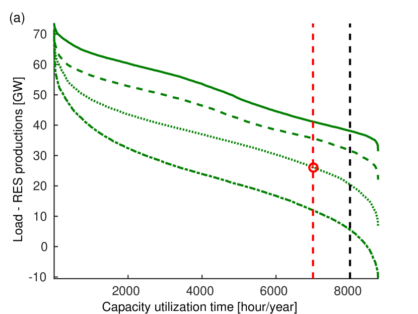
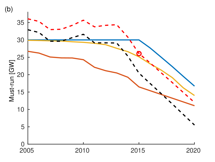
To obtain $R_{i}(t)$, we are left with evaluating the must-run power which is not a uniquely defined procedure (Schill, 2014; Denholm and Hand, 2011). To do so, we evaluate the must-run from duration curves which give the number of hours in a year that a given load is exceeded. Fig. 2 (a) shows duration curves for the total consumption minus the total RES production for four different years in Germany. We extract the must-run as the corresponding power threshold exceeded during ”most of the year”, and chose this to mean 7000 (vertical red dashed line) or 8000 hours (black dashed line). The obtained must-run is plotted in Fig. 2 (b) for these two choices (dashed lines). We see that the two curves mostly differ by a vertical shift of 3-4 GW. The must-run is about 30-35 GW in 2010, and keeps decreasing thereafter, as the penetration of RES increases and thermal plants are phased out.

Figure 2: (a) Duration curves of German load minus RES productions for the years 2000 (solid), 2010 (dashed), 2015 (dotted) and 2020 (dash-dotted). (b) Must run power as obtained from the duration curves [red and black dashed curves, corresponding to the red/black dashed vertical lines in panel (a)] and our three scenarios: keeping thermal production capacity ”as long as possible” (blue), ”exact substitution” of thermal production with new RES production (red), and smooth, in-between ”interpolated path” (orange). The red circles illustrate the connection between panel (a) and panel (b).

This is not the only possible procedure to evaluate the must-run but it agrees well with another, altogether different method. Nicolosi (2010) plots electricity prices hour by hour as a function of the percentage of the used production capacity for various types of production in Germany, from October 2008 to November 2009. The resulting cloud is rather elongated in all cases – and a linear regression is qualitatively representative of the data. From this linear regression, we may define the must-run as the capacity still used when this linear regression intersects the horizontal axis between positive and negative prices. One obtains a must-run corresponding to $85\%$ of the total nuclear capacity, $70\%$ of the total capacity of lignite power plants and $10\%$ of the total capacity of hard coal power plant. This estimate sums up to about 30-35 GW for 2010 in Germany, in agreement with our estimate extracted from duration curves. We therefore validate our procedure for estimating the volume of must-run production and use it to compute residual loads based on the scenario 2020 Expected progress of ENTSO-E (2015b).

It is important to realize that the procedure just described underestimates (overestimates) the must-run for exporting (importing) countries. As a matter of fact, Fig. 2 (b) suggests that the German must-run started to decrease already in 2013, instead, Germany’s thermal production capacity has been kept constant in 2013–2016 while its exports have increased significantly. This suggests that Germany will keep a large must-run as long as it can export its production when needed. To take this effect into account, we introduce three different scenarios for must-run evolution which we will use in our investigations. These three scenarios are shown in blue, orange and red in Fig. 2 (b). The blue curve corresponds to a must-run that is constant until 2015 after which it decreases with the same rate of $3$ [GW/year] in 2016-2020 as the dashed lines. The red curve corresponds to the opposite case where thermal capacities are withdrawn exactly at the same rate as new RES are installed. Finally, the orange curve is a smooth curve interpolating somehow arbitrarily between the blue and red scenarios. Below, we dub these three scenarios as long as possible (blue), interpolated path (orange) and exact substitution (red). We use these scenarios to investigate what ingredient(s) determine(s) the evolution of electricity prices. None of them is actually realized, however investigating the three of them allows to understand quantitatively the influence of must-run on electricity prices.

While we just focused on the German case to describe the procedure for evaluating must-run capacity, the described method is applied below to other European countries.

3 Electricity day-ahead markets

In the liberalized European electricity market, day-ahead transactions correspond to a significant share of the total consumed electricity. This is shown in Table 1. This share is expected to keep increasing in the future as the remaining long-term contracts expire, presumably with at most partial renewal because of market liberalization. In the next section we show the strong correlation between the residual load and the day-ahead price, which allows us to model future day-ahead prices. Given the sizeable share of day-ahead transactions, a share that will keep increasing in the coming years, we argue that this model gives us a faithful, qualitative model for future electricity prices (not only day-ahead).

Market zone	Traded energy	Load percentage
	[TWh]	[%]
AT / DE	264	53
BE	24	29
CH	23	38
CZ	20	28
ES / PT	259	79
FR	106	23
IT	195	62
NL	43	39
NO	133	103
PL	24	18
SE	128	94
UK	47	19
Total	1264	49

Table 1: Traded electrical energy and corresponding load percentage of several European day-ahead markets in 2015. Sources: EPEX SPOT (2015), OMIE (2015), OTE (2015) and NordPool (2015).

4 Correlations between residual loads and day-ahead prices

Fig. 1 illustrates the strong correlation between national residual loads $R_{i}(t)$ and day-ahead prices $p_{\mathrm{da}i}(t)$, a correlation that had been noticed by von Roon and Huber (2010) for Germany in 2007–2009. In this section, we further quantify this correlation for other European countries. Statistical correlation between discrete sets of data $X=\{x_{k}\}$ and $Y=\{y_{k}\}$ is standardly measured by Pearson’s correlation coefficient

$$r(X,Y)=\frac{\sum_{k=1}^{n}(x_{k}-\bar{x})(y_{k}-\bar{y})}{\sqrt{\sum_{k=1}^{n}(x_{k}-\bar{x})^{2}\sum_{k=1}^{n}(y_{k}-\bar{y})^{2}}},$$ (4.1)

where $\bar{x}$ and $\bar{y}$ are the average values of the two sets. By definition, one has $r\in[-1,1]$, with $r=0$ indicating the absence of correlation between the two sets, $r=1$ two perfectly correlated sets and $r=-1$ two totally anticorrelated sets. A value $r>0.5$ indicates an already strong correlation.

We calculate Pearson’s coefficient for different years and different European countries, based on their residual loads constructed as described in Section 2. For each reported year, we used hourly sets of data for both residual loads and day-ahead prices, from which we removed the 2 % highest and lowest values – corresponding to those that are further away from the average than between two and three standard deviations. These extreme events correspond to exceptional situations with forecast errors, unplanned production outages and so forth (CREG, 2015; Christensen et al., 2012), events that are hardly predictable and lay beyond the scope of the present manuscript. Table 2 shows the evolution of correlations between residual loads and day-ahead prices of the four largest countries in continental Europe. All values are large, $r>0.58$, and seem to be constant or perhaps even increasing with time

$r(p_{\mathrm{da}i},R_{i})$	2012	2013	2014	2015
FR	0.65	0.74	0.71	0.67
DE	0.78	0.86	0.89	0.89
IT	0.63	0.58	0.61	0.77
ES	#	#	0.77	0.88

Table 2: Evolution of the correlation between national day-ahead prices and residual loads.

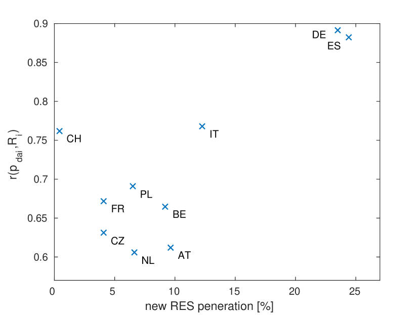
We further investigate the correlation coefficient for 2015 data in a number of continental European countries. Fig. 3 plots the correlation coefficient between national residual load and day-ahead electricity price as a function of new RES penetration, which we took as the ratio of yearly RES production to the total electricity production. Data are taken from ENTSO-E (2015a) and have been crosschecked and completed where necessary with data obtained from national grid operators and power markets.

The correlation coefficients in Table 2 and Fig. 3 satisfy $r(p_{\mathrm{da}i},R_{i})>0.58$ in all cases, indicating a strong correlation between the residual loads and day-ahead prices. Additionally, $r(p_{\mathrm{da}i},R_{i})$ is larger in countries with larger penetration of new RES (see Fig. 3), with the exception of Switzerland, where the correlation is presumably higher due to a large penetration of hydroelectricity - an ”old” RES. Given this trend, and the planned increase in new RES penetration in all European countries, it seems natural to expect an even larger correlation between residual loads and day-ahead prices in the future.

Figure 3: Pearson’s correlation coefficient $r$ between national residual loads $R_{i}$ and 2015 national day-ahead prices $p_{\mathrm{da}i}$ as a function of the penetration of new RES in several European countries.

5 Present and future electricity prices modeled after the residual load

We argued in Section 4 that the already large correlation factor $r$ between day-ahead prices and residual loads (see Table 2) is expected to become even larger as the penetration of new RES increases. This is so, because, as is illustrated in Fig. 3, $r$ is larger in countries with larger amounts of new RES. Simultaneously, day-ahead markets represent a significant part of all electricity transactions as is shown in Table 1, a share that is likely to keep increasing in Europe as the liberalization of the market becomes complete. It therefore makes sense to model future electricity prices from residual loads. The latter are based solely on scenarios for the evolution of the consumption, the future RES productions and the must-run. The economic feasibility and the future of different production types under given scenarios can then be checked quantitatively. In this section we construct such a price and show that it reproduces historical prices with very good accuracy, except for rare extreme events.

We construct a synthetic electricity price as a linear regression of the residual load,

$$p_{\mathrm{da}}(t)=\Delta p_{\mathrm{da}}R(t)+p_{\mathrm{da}0}\,,$$ (5.1)

where we rewrote Eq. (1.1). For the sake of simplicity, we drop the country index $i$ here. We focus on electricity prices and revenues for various productions in Spain and Germany, two large European countries that are already well engaged in their energy transition in the electric sector, with large penetration of new RES. The RES mix has proportionally less PV in Spain than in Germany, which allows us to identify differences in the evolution of prices from different choices of RES mixes. Based on 2015 data, we obtain $\Delta p_{\mathrm{da}}\approx 1$ and $2.2$ [€/MWh$\cdot$GW^-1] and $p_{\mathrm{da}0}\approx 20$ and $30$ [€/MWh] in Germany and Spain respectively for the parameters in Eq. (5.1). We found very little change in these parameters during the years 2013–2015 in Germany and therefore assume these parameters to be constant in time in each country, for a time window ranging from 2015 to 2020. That this is reasonable is illustrated in Fig. 4 which shows that the effective price $p_{\mathrm{da}}(t)$ of Eq. (5.1) reproduces historical day-ahead prices quite well. The agreement is already good in 2006 and becomes even better in 2013. Exceptional price spikes and troughs are not totally captured, which correspond however to unusual situations beyond the reach of our modeling.

Figure 4: Electricity price (5.1) built on the residual load (green line) and actual day-ahead electricity price (blue line) during a week in winter and summer 2006 (top two panels) and 2013 (bottom two panels) in Germany. Dashed lines show the monthly average price and the dotted-dashed lines prices exceeded 10 and 90 % of the time during that month. Vertical dashed lines indicate noon time.

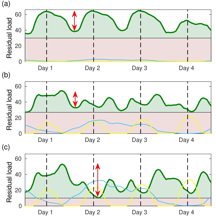
Eq. (5.1) allows us to qualitatively forecast electricity prices and price fluctuations in the framework of the energy transition. The latter substitutes thermal productions with new RES. Doing so, it reduces the must-run and changes fluctuations in the residual load. The way these fluctuations change depends on the chosen RES mix: PV produces more around noon, it therefore is correlated with the main load peak; WT production on the other hand is effectively random in time on time scales of the order of few hours to few days, and therefore uncorrelated with consumption on such time scales. Consequently, fluctuations in residual loads will always increase if the substitution mix is made of WT only, while they will first decrease before increasing again if the mix is dominated by PV. This is illustrated in Fig. 5 which sketches the behavior of the residual load at three different stages of the energy transition. Panel (a) shows the situation at the very initial stage of the energy transition, with low RES penetration. The shape of the residual load is very similar to the load itself and the must-run is high. Panel (b) illustrates the transition period with increased RES penetration with a significant fraction of PV, corresponding to the German mix. PV significantly decreases the load peak during office hours, which reduces fluctuations of the residual load. The must-run is still high. In our model, this reduces fluctuations in electricity prices, therefore there are less financial opportunities for flexible productions. In the final stages of the energy transition, the large RES penetration completely changes the shape of the residual load, which looks now very different from the load, see Fig. 5 (c). The must-run power is lower, bringing average prices higher. Most importantly, fluctuations in the residual load are comparable to and even higher than those at the early stages of the energy transition.

Figure 5: Sketch of the residual load (green area) and must-run (light red band) at three stages of the energy transition: (a) Initial, (b) intermediate and (c) late stages of the transition. PV (yellow) and WT (light blue) production profiles are superimposed. Red arrows indicate the magnitude of fluctuations of the residual load. Vertical dashed lines indicate noon time.

The residual load quantifies the balance between non-flexible supply and demand, and accordingly, the correlation between electricity prices and residual load can be understood as a logical consequence of the economic law of supply and demand. This correlation may vary in the future, however, from fundamental laws of economics, it is likely to remain sizeable in any event. It therefore makes sense to introduce an electricity price as in Eq. (5.1). Varying economic conditions may however impact the pricing parameters $\Delta p_{\mathrm{da}}$ and $p_{\mathrm{da}0}$ and there is no reason a priori to consider them constant in time (the scenario we discuss in this manuscript). Other scenarios with varying $\Delta p_{\mathrm{da}}$ and $p_{\mathrm{da}0}$ can be investigated. Qualitatively, one anticipates that $p_{\mathrm{da}0}$ is determined by the marginal cost of must-run production. In Europe this is essentially the marginal price of electricity from coal-fired plants, and therefore $p_{\mathrm{da}0}$ increases if carbon taxes increase. The parameter $\Delta p_{\mathrm{da}}$ on the other hand is more directly related to the order of merit, and thus to the marginal cost of electriciy from gas-fired power plants. As such it will follow the evolution of both carbon taxes and natural gas prices. How much these parameters vary for given variations in gas prices and carbon taxes needs to be calibrated. Performing this calibration goes beyond the purpose of the present manuscript and is left to future works. Here, we consider constant $\Delta p_{\mathrm{da}}$ and $p_{\mathrm{da}0}$ and restrict our investigations to a relatively short time window, until 2020.

With these considerations, and under the assumptions described above, it is easy to qualitatively predict the evolution of electric revenues. Consider for instance a high-power pumped-storage (PS) hydroelectric plant. Its revenues directly depend on the difference between highest and lowest prices. From the discussion above, a PS plant sees its revenue first decrease in the initial stages of the energy transition, where increased RES penetration reduces price fluctuations. The revenue however increases later, once the RES penetration is such that it restores large fluctuations in residual loads and thus in electricity prices. In the upcoming sections we show that the intermediate period of reduced revenues for flexible productions depends on (i) the rate at which RES penetration increases, (ii) the chosen RES mix, and (iii) the rate at which must-run is reduced. To overcome the paradox of the energy transition, one needs to chose scenarios such that these three ingredients, when combined, reduce the duration of the intermediate period with low revenues.

6 Future revenues by electricity production type

We investigate the future revenues of different electricity productions in Europe with the synthetic electricity price of Eq. (5.1). We initially focus on the hydroelectric sector, which can provide flexibility of production and storage capacities needed to integrate new RES into the electric grid. We next turn our attention to general power plants characterized by their annual number of operation hours.

Figure 6: The actual (solid black curve) and computed (dotted black curve) production of a typical Swiss PS plant and the day-ahead price (blue curve). Negative production means pump load. Sources: Swissgrid and ENTSO-E (2015a).

6.1 Revenues of a pumped-storage plant and the fluctuations of the residual load

The revenue $G$ of a PS plant over a time interval $t\in[t_{i},t_{f}]$ is given by

$$G=\int_{t_{i}}^{t_{f}}p_{\mathrm{da}}(t)\cdot P_{\mathrm{PS}}(t)\mathrm{d}t,$$ (6.1)

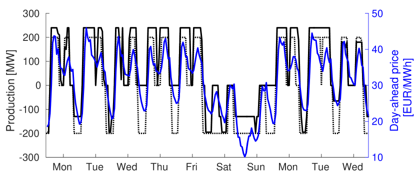
where $P_{\mathrm{PS}}(t)$ is the electric power produced ($P_{\mathrm{PS}}(t)>0$) or consumed ($P_{\mathrm{PS}}(t)<0$) by the plant. Optimizing the revenue of PS plants means producing when $p_{\mathrm{da}}(t)$ is large and consuming when $p_{\mathrm{da}}(t)$ is low. It therefore makes sense to assume that $P_{\mathrm{PS}}$ and $p_{\mathrm{da}}$ are strongly correlated. This assumption is confirmed in Fig. 6, which shows the production of a Swiss PS plant and the day-ahead price for 10 consecutive days in 2015. Neglecting losses for the time being, we write

$$P_{\mathrm{PS}}(t)\cong\pi_{\mathrm{PS}}\cdot[p_{\mathrm{da}}(t)-\bar{p}_{\mathrm{da}}],$$ (6.2)

where $\bar{p}_{\mathrm{da}}$ is the average price over the considered time period and $\pi_{\mathrm{PS}}$ is a prefactor linking prices to production. Eq. (6.2) guarantees that $\int_{t_{i}}^{t_{f}}P_{\mathrm{PS}}(t)\mathrm{d}t=0$ as should be for a PS plant without loss. Inserting Eq. (6.2) into (6.1) and using Eq. (5.1), we get

$$G\cong\pi_{\mathrm{PS}}\,\Delta p^{2}_{\mathrm{da}}\,T\,\mathrm{Var}[R]\,,$$ (6.3)

for the annual revenue with $T=8760$ hours. This result shows that the revenue of a lossless PS plant is proportional to the variance of the residual load. Eq. (6.3) formalizes the relation qualitatively discussed at the end of Section 5 between revenues of PS plants and fluctuations of the residual load.

Figure 7: (a) Normalized revenue (divided by the revenue of 2005 in the scenario ”as long as possible”) of a German PS plant with $\eta=0.9$, for different scenarios of must-run withdrawal (see Section 2) : ”as long as possible” (blue), ”interpolated path” (orange) and ”exact substitution” (red). (b) Evolution of WT (light blue) and PV (yellow) annual production in Germany. Dashed rectangles correspond to planned future evolution (ENTSO-E, 2015b).

6.2 Future revenues of a pumped-storage plant

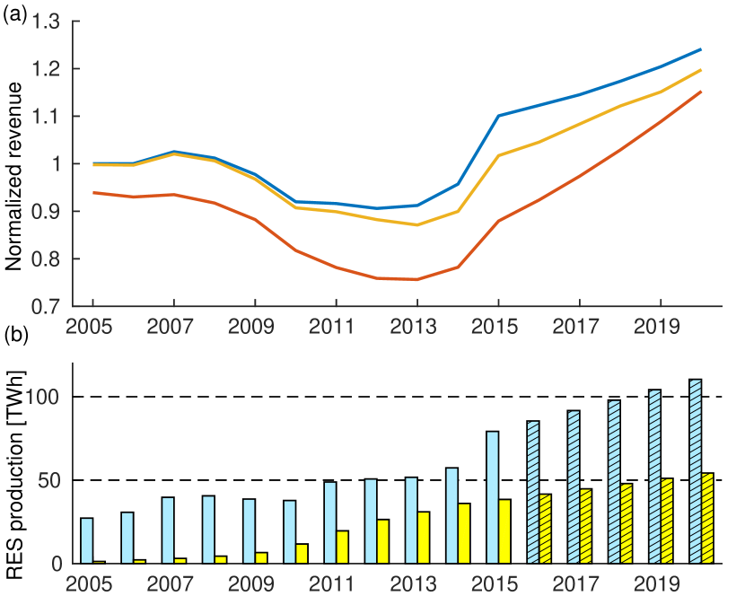
We next investigate numerically the revenue of PS plants in Germany and Spain in the period 2005-2020. Residual loads are calculated from 2015 data for the load and RES profiles, the latter being scaled up from year to year to interpolate linearly between the 2015 realized annual production and the planned 2020 annual production (ENTSO-E, 2015b). The evolution of the annual RES productions is given in Figs. 7 (b) and 8 (b). The revenue is given by

$$G =\sum_{k}p_{\mathrm{da},k}\,P_{\mathrm{PS},k}\,\Delta t=\sum_{k}p_{\mathrm{da},k}[P_{\mathrm{t},k}-P_{\mathrm{p},k}]\,\Delta t\,,$$ (6.4)

with the time step $\Delta t$ used in the calculation – one hour in our case – and where we introduced $P_{\mathrm{PS},k}=-P_{\mathrm{p},k}$ when $P_{\mathrm{PS},k}<0$ and $P_{\mathrm{PS},k}=P_{\mathrm{t},k}$ when $P_{\mathrm{PS},k}>0$. The power profile is related to the evolution of the reservoir level $S_{\mathrm{PS},k}$, and for a PS plant with pump/turbine efficiency $0\leq\eta\leq 1$ each way, this relation reads

$$S_{\mathrm{PS},k+1}=S_{\mathrm{PS},k}+[\eta P_{\mathrm{p},k}-\eta^{-1}P_{\mathrm{t},k}]\Delta t\,.$$ (6.5)

Finally, the reservoir level must be positive but smaller than its maximal level at all times, giving the constraint

$$0\leq S_{\mathrm{PS},k}\leq S_{\mathrm{PS}}^{\max}\,,\hskip 10.0pt\forall k.$$ (6.6)

Eqs. (6.4)–(6.6) govern the production of a PS plant. We generate PS power profiles by maximizing the revenue $G$ of Eq. (6.4) under the constraints of Eqs. (6.5) and (6.6). Using the actual day-ahead price, this procedure generates a fictitious PS production profile given by the dotted black curve in Fig. 6, which is very close to the actual one (solid black curve). We attribute the few discrepancies to the fact that our maximization of $G$ in Eq. (6.4) is made with perfect advance knowledge of the load and RES productions. This test substantiates our procedure for calculating power profiles and evaluating revenues of PS plants.

Figure 8: (a) Normalized revenue (divided by the revenue of 2005 in the scenario ”as long as possible”) of a Spanish PS plant with $\eta=0.9$, for different scenarios of must-run withdrawal (see Section 2) : ”as long as possible” (blue), ”interpolated path” (orange) and ”exact substitution” (red). (b) Evolution of WT (light blue) and PV (yellow) annual production in Spain. Dashed rectangles correspond to planned future evolution (ENTSO-E, 2015b).

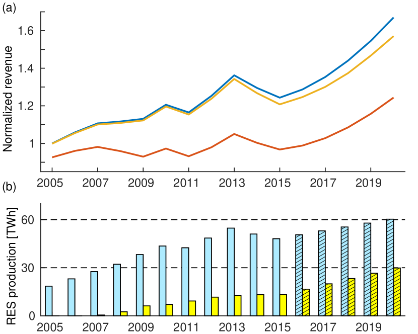
We calculate revenues of PS plants from Eqs. (6.4)–(6.6) with the synthetic price of Eq. (1.1) and the usually reported efficiency of $\eta=0.9$ each way (Rehman et al., 2015; Guittet et al., 2016). Revenues of German and Spanish PS plants as the energy transition unfolds are shown in Figs. 7 and 8. It is seen that they remain approximately constant in both countries from 2005 to 2008/2009, even though the WT production increases by 40 % in Germany and almost 50 % in Spain. Revenues decrease significantly in Germany from 2009 on, reaching a minimum around 2013 with revenues reduced by as much as 20 %. The revenues decrease more for faster must-run reduction [see Fig. 7 (a)]. This is easily understandable when one realizes that a higher must-run reduces the residual load, and with it, the electricity price. Power losses due to the finite efficiency of the plant, $\eta<1$, cost less at higher must-run, which increases revenues.

The striking feature in Fig. 7 (a) is that, as expected from the discussion in Section 5 together with Eq. (6.3), the drop in revenues corresponds to the acceleration of the penetration of PV, which reduces the mid-day residual load peak. The fluctuations of the residual load go down, leading to reduced revenues through Eq. (6.3). As the penetration of PV further increases, so do the fluctuations of the residual load – one enters the stage depicted in Fig. 5 (c) and the revenues increase again. The drop in revenues does not last long. The importance of PV in this phenomenon becomes clear when comparing Fig. 7 (a) and Fig. 8 (a). The latter figure displays no significant drop for a Spanish PS plant. This is so, because the mix of new RES is clearly dominated by WT in Spain. Fluctuations in residual load are increased at all stages of the transition, regardless of the chosen scenario for must-run reduction. Thus, from Eq. (6.3), revenues also always tend to increase.

6.3 Future revenues of conventional hydroelectric plants

We next consider conventional dam hydroelectric power plants. The main difference with PS plants is that (i) conventional dam hydroelectric plants only produce and (ii) their reservoir is filled by natural water inflow. We model them slightly differently from PS plants. Their revenue is given by

$$G =\sum_{k}p_{\mathrm{da},k}\,P_{\mathrm{D},k}\,.$$ (6.7)

We use the same synthetic price for $p_{\mathrm{da},k}$ in Eq. (6.7) as for the analysis of PS plants. The power profile $P_{\mathrm{D},k}$ is related to the evolution of the reservoir level $S_{\mathrm{D},k}$,

$$S_{\mathrm{D},k+1}=S_{\mathrm{D},k}+[I_{k}-P_{\mathrm{D},k}]\,\Delta t\,,$$ (6.8)

where $I_{k}$ is the power corresponding to water inflow into the dam (rain- and snowfall, snow- and icemelt) at the time interval $k$. The reservoir level must be positive but smaller than the maximal storage capacity at all times, giving a condition similar to (6.6),

$$0\leq S_{\mathrm{D},k}\leq S_{\mathrm{D}}^{\max}\,,\hskip 5.0pt\forall k\,.$$ (6.9)

As for PS power plants, we determine the power profile $P_{\mathrm{D},k}$ by maximizing the gain $G$ in Eq. (6.7) for a typical dam hydro power plant in the Alps. We take $\{I_{k}\}$ as the water inflow averaged over all Swiss dams, as extracted from weekly dam energy content and production (Swiss Federal Office of Energy, 2016). A conventional dam hydroelectric plant is characterized by its rated power $P_{\mathrm{D}}^{\max}$, its storage capacity $S_{\mathrm{D}}^{\max}$ and the annual energy inflow $E_{\mathrm{D}}=\sum_{k}I_{k}\Delta t$. Relative revenue evolution therefore depends on only two dimensionless parameters which we take as $S_{\mathrm{D}}^{\max}/P_{\mathrm{D}}^{\max}\Delta t\equiv N_{\rm empty}$ and $E_{\mathrm{D}}/P_{\mathrm{D}}^{\max}\Delta t\equiv N_{\rm op}$, giving the number of hours of operation at full power to empty the reservoir and to use all the annual energy inflow respectively. We found that revenues depend only very weakly on $N_{\rm empty}$, and therefore focus on the evolution of revenues vs. $N_{\rm op}$. In multiannual average, dams annually produce their energy inflow $E_{\mathrm{D}}$, and in continental Europe, this usually corresponds to $N_{\rm op}\in[1000,3000]$ hours of full power operation (Thürler, 2014).

Figure 9: Normalized revenue of conventional dam hydroelectric plants with high ($N_{\rm op}=1000$ hours; solid lines) and low ($N_{\rm op}=3000$ hours; dashed lines) power capacity in the Alps, with $N_{\rm empty}=1000$ hours and for the scenarios ”as long as possible” (blue), ”expected path” (orange) and ”exact substitution” (red) of must-run withdrawal.

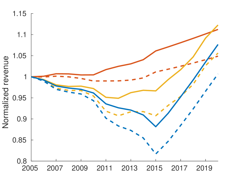
Fig. 9 shows the revenues of conventional dam hydroelectric plants with $N_{\rm empty}=1000$ and $N_{\rm op}=1000,3000$. One sees a similar nonmonotonous behavior as for PS plants in Germany (Fig. 7). How much and until when the revenue drops depend sharply on the chosen scenario for must-run withdrawal. Generally, we find that revenues drop more and longer for delayed must-run withdrawal – the flexibility of conventional dam hydroelectric power plants is rewarded best for exact substitution of production capacity, where production from thermal plants is reduced at the same rate as new RES production increases. Only in that case would we see no drop in revenue for conventional hydro power plants. Regardless of the must-run scenario, revenues go back to their pre-energy transition level by 2020 at the latest in all considered scenarios. We observe that plants with higher rated power $P_{\mathrm{D}}^{\max}$, i.e. lower number $N_{\rm op}$ of annual operation hours, see their revenue decrease less than those with lower power, because the higher the rated power, the easier it is to produce almost only during peaks of financial opportunities.

6.4 Future revenues of power plants by annual operation time

To understand better the trends discussed above, we finally investigate different types of productions characterized only by the number of hours $N_{\rm op}$ they operate at maximal power $P_{\mathrm{D}}^{\max}$ per year with no further constraint. Accordingly, we consider four classes of power plants which are (i) super-peaking plants, functioning $N_{\rm op}=$ 1000 hours per year at peak power, (ii) peaking plants $N_{\rm op}=2000$, (iii) load-following plants $N_{\rm op}=5000$ and (iv) base-load plants $N_{\rm op}=8000$. We calculate their revenues using Eq. (6.7), with the constraint $\sum_{k}P_{\mathrm{D},k}=P_{\mathrm{D}}^{\max}\,N_{\rm op}$. Fig. 10 shows the evolution of these revenues as the energy transition unfolds in Germany, for our three scenarios for must-run reduction. We see first, that regardless of must-run reduction, peak production plants always have higher revenues and second, that faster must-run withdrawal leads to smaller reductions in revenues. In particular, there is no significant decrease in revenue in the exact substitution scenario, for which thermal plants are retired in direct proportion to the penetration increase of new RES.

Figure 10: Normalized revenues of super-peaking plants (functioning 1000 hours/year at maximal power; solid lines), peaking plants (2000 hours/year; dashed lines), load-following plants (5000 hours/year; dotted-dashed lines) and base-load plants (8000 hours/year; dotted lines) under the three scenarios ”as long as possible” (panel a), ”expected path” (panel b), ”exact substitution” (panel c) of must-run withdrawal.

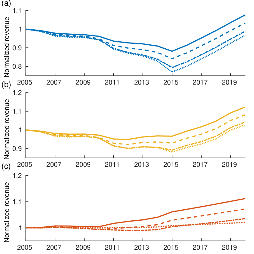
These results indicate that the currently very low electricity prices in Europe (and the poor revenues of the hydroelectricity sector) are due to an overcapacity of electricity production more than anything else. Thermal plants are currently retired too slowly compared to the rate at which the penetration of new RES increases. We therefore conjecture that the paradox of the energy transition can be overcome by retiring thermal plants faster.

7 Conclusions

Our interest in this manuscript has been to investigate the conditions under which the energy transition in the electric sector can proceed in Europe, without financially jeopardizing flexible productions. This is a key issue, since increasing the penetration of new RES in the continental European grid will eventually require sizeable power reserves that can be mobilized fast and often to compensate unavoidable, stochastic fluctuations in RES productions. Such reserves already exist (an example is hydroelectricity), however, they are currently under strong financial stress because of very low electricity prices. It is of paramount importance to figure out how long this stress will last and how it can be reduced in order to secure the future of flexible productions and with them, the harmonious unfolding of the energy transition. This is what we called ”overcoming the paradox of the energy transition”.

To investigate this issue, we constructed a physico-economic model of the European grid. We observed a strong correlation between day-ahead electricity prices and residual loads all over Europe, and from that correlation, we constructed an electricity price solely based on the residual load, Eqs. (1.1) and (5.1). This price enabled us to investigate future revenues of various types of power plants. We found that three ingredients determine the occurrence, magnitude and duration of the paradox of the energy transition: (i) the rate at which the energy transition proceeds and RES penetration is increased, (ii) the mix of new RES and (iii) the rate of must-run withdrawal. In particular, if the must-run is kept high as RES penetration increases, electricity prices go down with base prices well below the marginal cost of any flexible production. The hydroelectric sector in continental Europe is currently suffering from very low electricity prices, and our results indicate that this situation is mostly due to surplus must-run capacity. The duration of this paradoxical situation will decisively depend on how fast surplus thermal production capacities are withdrawn to compensate for the increased production from new RES. We advocate a faster withdrawal, for instance by substituting flexible gas-powered plants for coal-fired plants, which would additionally reduce greenhouse gas emissions faster.

The energy transition is accompanied by an increased need of production flexibility as it proceeds. Plants with large power will be needed more frequently, and it is expectable that they will operate on a peak mode with 2000 hours of operation per year or less. It may well be that different business plans will be developed for such plants, with different financial tools to reward not the energy produced, but the ancillary services provided. How such incentives will be introduced remains speculative. Our results suggest that, even without them, peak and super-peak power plants should soon benefit again from improved financial conditions.

As a final comment we note that different scenarios with different consumption curves can be investigated with the model presented above. In particular, active demand response can be incorporated into the model, as we discuss in A.

Appendix A Incorporating active demand response

We sketch how active demand response (ADR) can be incorporated into our model. With ADR, the residual load is given by

$$R(t)=L(t)+\delta L(t)-P^{\rm PV}(t)-P^{WT}(t)-P^{\rm MR}=R_{0}(t)+\delta L(t)\,,$$ (A.1)

where changes in the load profile due to ADR are included in $\delta L(t)$ and $R_{0}$ is the residual load without ADR, as in Eq. (2.1). ADR can be deployed for various reasons, for instance to reduce electricity costs of end users or to mitigate load fluctuations on the distribution network. In both instances, ADR tries to reduce variations in the residual load, and we incorporate this goal in an optimizing procedure which we briefly describe. For the sake of simplicity, we do not incorporate specific load constraints such as comfort temperature intervals for ADR with thermostatically controlled loads. The only constraint on the ADR profile is

$$\big{|}\delta L(t)\big{|}<\delta L^{\max}\,,\forall t\,,$$ (A.2)

where $\delta L^{\max}$ is the maximal ADR power. We further assume that the annual consumption remains unchanged,

$$\intop_{t_{i}}^{t_{f}}\delta L(t){\rm d}t=0\,.$$ (A.3)

Recent estimates of the potential of ADR indicate that only a fraction of the total consumption can be shifted,

$$\intop_{t_{i}}^{t_{f}}\big{|}\delta L(t)\big{|}{\rm d}t\leq 2\sigma\intop_{t_{i}}^{t_{f}}L(t){\rm d}t\,,$$ (A.4)

with $\sigma\simeq 0.01$ giving the maximal fraction of the total consumption that can been shifted, while the maximal ADR power $\delta L^{\max}$ is about 10 % of the maximal load $L^{\max}$ (roughly corresponding to 7 GW in Germany) (Gils, 2016). These numbers may seem rather small, however they have been obtained assuming a broad load participation in ADR (Gils, 2016).

Our procedure is to compute the ADR profile that minimizes the fluctuations of the residual load,

$$\underset{\delta L}{\min}\big{[}\mathrm{Var}(R)\big{]}=\underset{\delta L}{\min}\big{[}\mathrm{Var}(L^{+}-L^{-}+R_{0})\big{]}\,,$$ (A.5)

where we defined $L^{\pm}(t)={\rm max}[0,\pm\delta L(t)]$. We linearly increase $\sigma$ and $\delta L^{\max}/L^{\max}$ from 0 in 2015 to $\sigma=0.01$ and $\delta L^{\max}/L^{\max}=0.1$ in 2025. Because we neglect specific load constraints on ADR, our results likely overestimate the impact of ADR on the residual load, and therefore on electricity prices.

Fig. 11 (a) shows the effect of ADR on the revenues of a PS plant. ADR being a form of storage, it competes with PS and reduces its revenues, however, the effect is rather moderate, with 2020 revenues still exceeding those of 2005. Fig. 11 (b) shows the revenues of a conventional dam hydroelectric plant, which are even less affected by ADR than those of the PS plant.

Figure 11: (a) Revenues of a PS plant in Germany with (plain) and without (dashed) ADR. (b) Revenues of a conventional dam hydroelectric plant in Germany with (plain) and without (dashed) ADR. ADR linearly evolves from zero in 2015 to its maximal potential in 2025, with $\delta L^{\max}=7$[GW] and $\sigma=0.01$ (Gils, 2016).

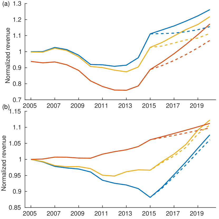
Qualitatively, our conclusions stated in the main text remain valid.

References

- Auer and Haas (2016) Auer, H., Haas, R., 2016. On integrating large shares of variable renewables into the electricity system. Energy 115, 1592–1601.
- Christensen et al. (2012) Christensen, T. M., Hurn, A. S., Lindsay, K. A., 2012. Forecasting spikes in electricity prices. International Journal of Forecasting 28, 400–411.
- Clò et al. (2015) Clò, S., Cataldi, A., Zoppoli, P., 2015. The merit-order effect in the Italian power market: The impact of solar and wind generation on national wholesale electricity prices. Energy Policy 77, 79–88.
- Cludius et al. (2014) Cludius, J., Hermann, H., Matthes, F. C., Graichen, V., 2014. The merit order effect of wind and photovoltaic electricity generation in Germany 2008–2016: Estimation and distributional implications. Energy Economics 44, 302–313.
- CREG (2015) CREG, 2015. The price spikes observed on the Belgian day-ahead spot exchange Belpex on 22 September and 16 October 2015. Tech. rep., Commission for electricity and gas regulation.
- Denholm and Hand (2011) Denholm, P., Hand, M., 2011. Grid flexibility and storage required to achieve very high penetration of variable renewable electricity. Energy Policy 39, 1817–1830.
- ENTSO-E (2015a) ENTSO-E, 2015a. ENTSO-E Transparency platform. https://transparency.entsoe.eu/.
- ENTSO-E (2015b) ENTSO-E, 2015b. TYNDP 2016: Scenario Development Report.
- EPEX SPOT (2015) EPEX SPOT, 2015. Annual report. https://www.epexspot.com/en/extras/download-center/activity_reports.
- Guittet et al. (2016) Guittet, M., Capezzali, M., Gaudard, L., Romerio, F., Vuille, F., Avellan, F., 2016. Study of the drivers and asset management of pumped-storage power plants historical and geographical perspective. Energy 111, 560–579.
- Haas et al. (2013) Haas, R., Lettner, G., Auer, H., Neven, D., 2013. The looming revolution: how photovoltaics will change electricity markets in europe fundamentally. Energy 57, 38–43.
- Nicolosi (2010) Nicolosi, M., 2010. Wind power integration and power system flexibility – An empirical analysis of extreme events in Germany under the new negative price regime. Energy Policy 38, 7257–7268.
- Nicolosi (2012) Nicolosi, M., 2012. The economics of renewable electricity market integration. an empirical and model-based analysis of regulatory frameworks and their impacts on the power market. Ph.D. thesis, Universität zu Köln.
- NordPool (2015) NordPool, 2015. Annual report. http://www.nordpoolspot.com/About-us/Annual-report/.
- OMIE (2015) OMIE, 2015. Main results of the electricity market. http://www.omie.es/files/mercado_electrico_ing.diptico_web_pdf.pdf.
- OTE (2015) OTE, 2015. Annual report. http://www.ote-cr.cz/about-ote/annual-reports.
- Pagnier and Jacquod (2017) Pagnier, L., Jacquod, P., 2017. A predictive pan-european economic and production dispatch model for the energy transition in the electricity sector. In: PowerTech, 2017 IEEE Manchester. IEEE.
- Paraschiv et al. (2014) Paraschiv, F., Erni, D., Pietsch, R., 2014. The impact of renewable energies on EEX day-ahead electricity prices. Energy Policy 73, 196–210.
- Rehman et al. (2015) Rehman, S., Al-Hadhrami, L. M., Alam, M. M., 2015. Pumped hydro energy storage system: A technological review. Renewable and Sustainable Energy Reviews 44, 586–598.
- Saarinen et al. (2015) Saarinen, L., Dahlbäck, N., Lundin, U., 2015. Power system flexibility need induced by wind and solar power intermittency on time scales of 1–14 days. Renewable Energy 83, 339–344.
- Schill (2014) Schill, W.-P., 2014. Residual load, renewable surplus generation and storage requirements in germany. Energy Policy 73, 65–79.
- Schlachtberger et al. (2016) Schlachtberger, D. P., Becker, S., Schramm, S., Greiner, M., 2016. Backup flexibility classes in emerging large-scale renewable electricity systems. Energy Conversion and Management 125, 336–346.
- Schweiger et al. (2017) Schweiger, G., Rantzer, J., Ericsson, K., Leuenburg, P., 2017. The potential of power-to-heat in Swedish district heating systems. Energy, in Press.
- Sensfuss et al. (2008) Sensfuss, F., Ragwitz, M., Genoese, M., 2008. The merit-order effect: A detailed analysis of the price effect of renewable electricity generation on spot market prices in Germany. Energy policy 36, 3086–3094.
- Swiss Federal Office of Energy (2016) Swiss Federal Office of Energy, 2016. Weekly report on water level of reservoirs. http://www.bfe.admin.ch/themen/00526/00541/00542/00630/index.html?lang=en&dossier_id=00766.
- Thürler (2014) Thürler, G., 2014. Statistik der Wasserkraftanlagen der Schweiz. http://www.bfe.admin.ch/themen/00490/00491/index.html?lang=de&dossier_id=01049.
- Ueckerdt et al. (2015) Ueckerdt, F., Brecha, R., Luderer, G., Sullivan, P., Schmid, E., Bauer, N., Böttger, D., Pietzcker, R., 2015. Representing power sector variability and the integration of variable renewables in long-term energy-economy models using residual load duration curves. Energy 90, 1799–1814.
- von Roon and Huber (2010) von Roon, S., Huber, M., 2010. Modeling spot market pricing with the residual load. Tech. rep., Forschungsstelle für Energiewirtschaft.
- Gils (2016) Gils, H. C., 2016. Economic potential for future demand response in Germany–modeling approach and case study. Applied Energy 162, 401–415.