On the asymptotic approximation to the probability distribution of extremal precipitation

Abstract. Based on the negative binomial model for the duration of wet periods measured in days [2], an asymptotic approximation is proposed for the distribution of the maximum daily precipitation volume within a wet period. This approximation has the form of a scale mixture of the Fréchet distribution with the gamma mixing distribution and coincides with the distribution of a positive power of a random variable having the Snedecor–Fisher distribution. The proof of this result is based on the representation of the negative binomial distribution as a mixed geometric (and hence, mixed Poisson) distribution [7] and limit theorems for extreme order statistics in samples with random sizes having mixed Poisson distributions [22]. Some analytic properties of the obtained limit distribution are described. In particular, it is demonstrated that under certain conditions the limit distribution is mixed exponential and hence, is infinitely divisible. It is shown that under the same conditions the limit distribution can be represented as a scale mixture of stable or Weibull or Pareto or folded normal laws. The corresponding product representations for the limit random variable can be used for its computer simulation. Several methods are proposed for the estimation of the parameters of the distribution of the maximum daily precipitation volume. The results of fitting this distribution to real data are presented illustrating high adequacy of the proposed model. The obtained mixture representations for the limit laws and the corresponding asymptotic approximations provide better insight into the nature of mixed probability (“Bayesian”) models.

Key words: wet period, maximum daily precipitation, negative binomial distribution, asymptotic approximation, extreme order statistic, random sample size, gamma distribution, Fréchet distribution, Snedecor–Fisher distribution, parameter estimation.

1 Introduction

In most papers dealing with the statistical analysis of meteorological data available to the authors, the suggested analytical models for the observed statistical regularities in precipitation are rather ideal and inadequate. For example, it is traditionally assumed that the duration of a wet period (the number of subsequent wet days) follows the geometric distribution (for example, see [1]) although the goodness-of-fit of this model is far from being admissible. Perhaps, this prejudice is based on the conventional interpretation of the geometric distribution in terms of the Bernoulli trials as the distribution of the number of subsequent wet days (“successes”) till the first dry day (“failure”). But the framework of Bernoulli trials assumes that the trials are independent whereas a thorough statistical analysis of precipitation data registered in different points demonstrates that the sequence of dry and wet days is not only independent, but it is also devoid of the Markov property so that the framework of Bernoulli trials is absolutely inadequate for analyzing meteorological data.

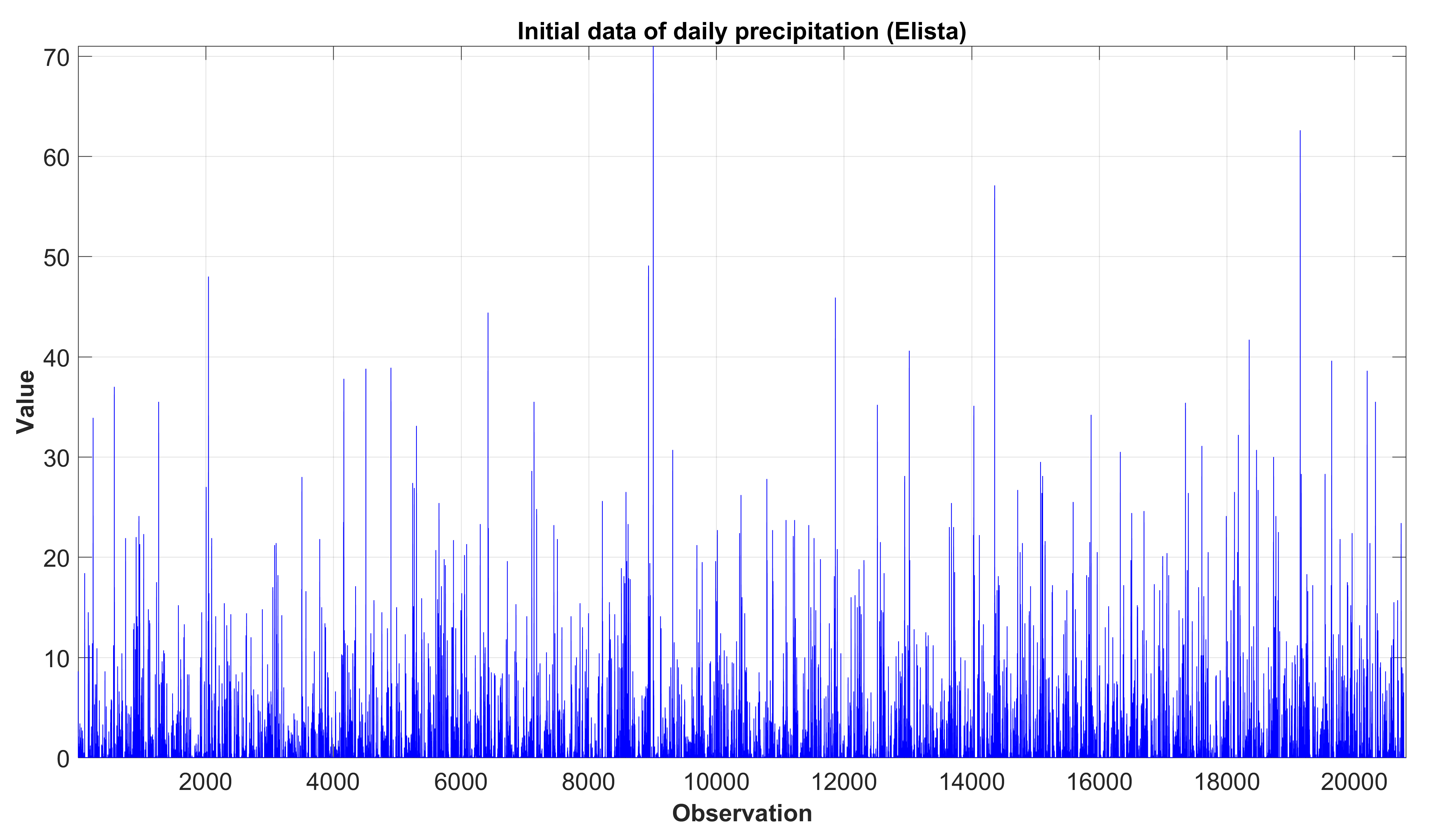
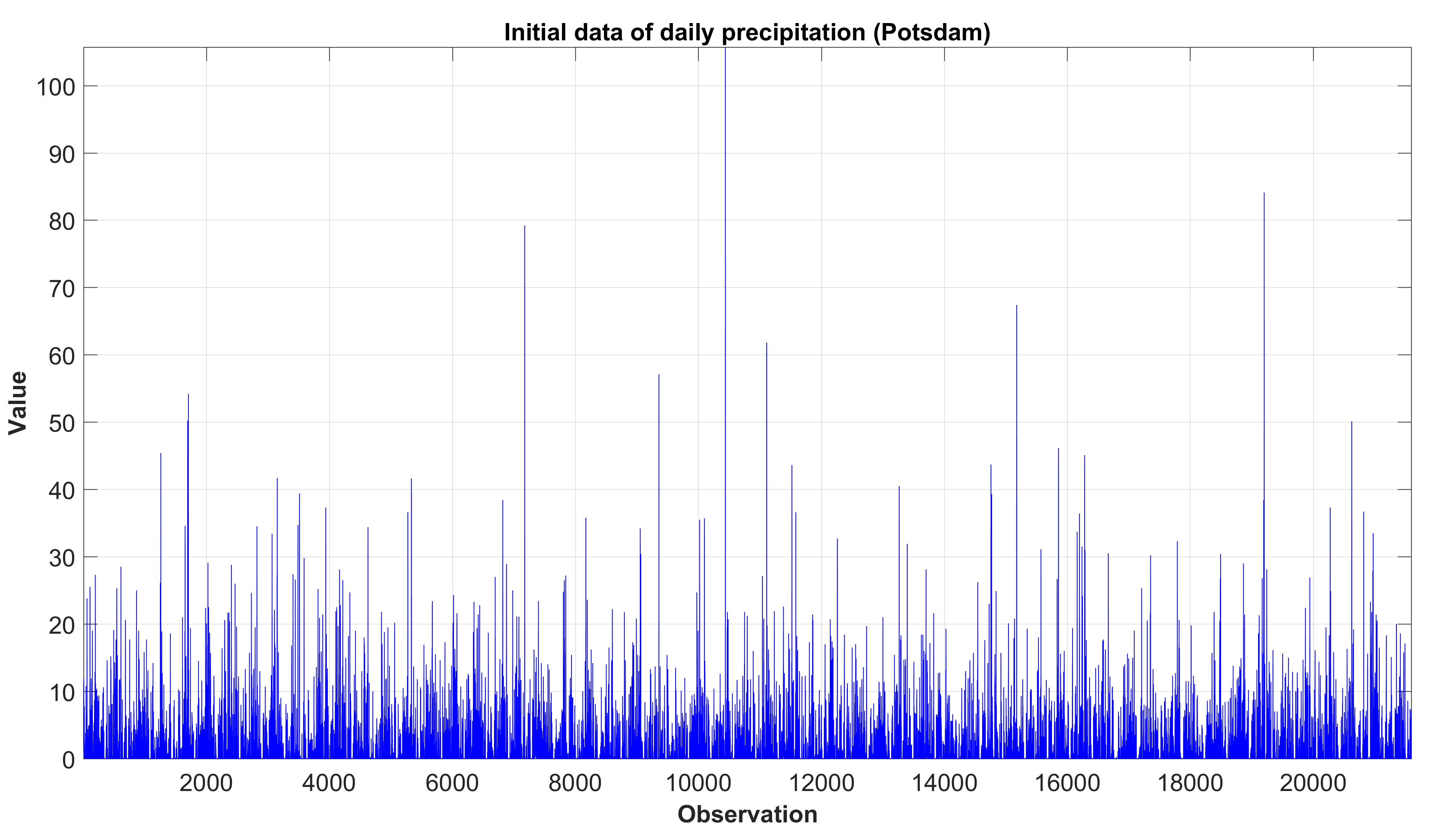
It turned out that the statistical regularities of the number of subsequent wet days can be very reliably modeled by the negative binomial distribution with the shape parameter less than one. For example, in [2] we analyzed meteorological data registered at two geographic points with very different climate: Potsdam (Brandenburg, Germany) with mild climate influenced by the closeness to the ocean with warm Gulfstream flow and Elista (Kalmykia, Russia) with radically continental climate. The initial data of daily precipitation in Elista and Potsdam are presented on Figures 1a and 1b, respectively. On these figures the horizontal axis is discrete time measured in days. The vertical axis is the daily precipitation volume measured in centimeters. In other words, the height of each “pin” on these figures is the precipitation volume registered at the corresponding day (at the corresponding point on the horizontal axis).

a)

b)

Fig. 1: The initial data of daily precipitation in Elista (a) and Potsdam (b).

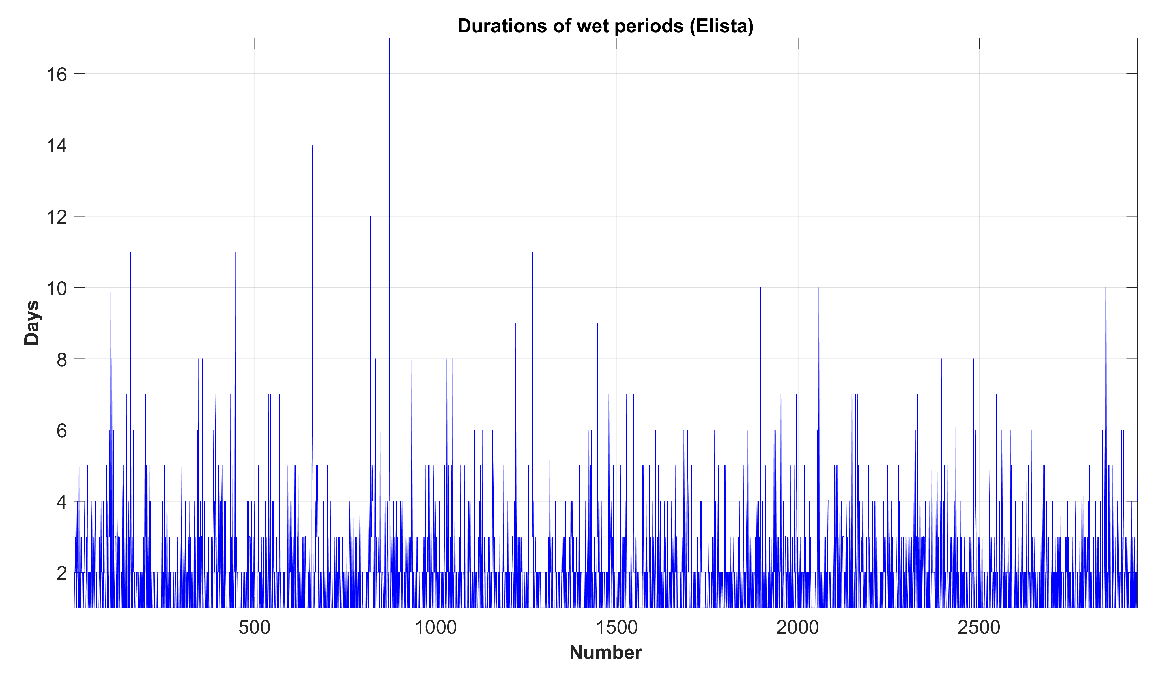
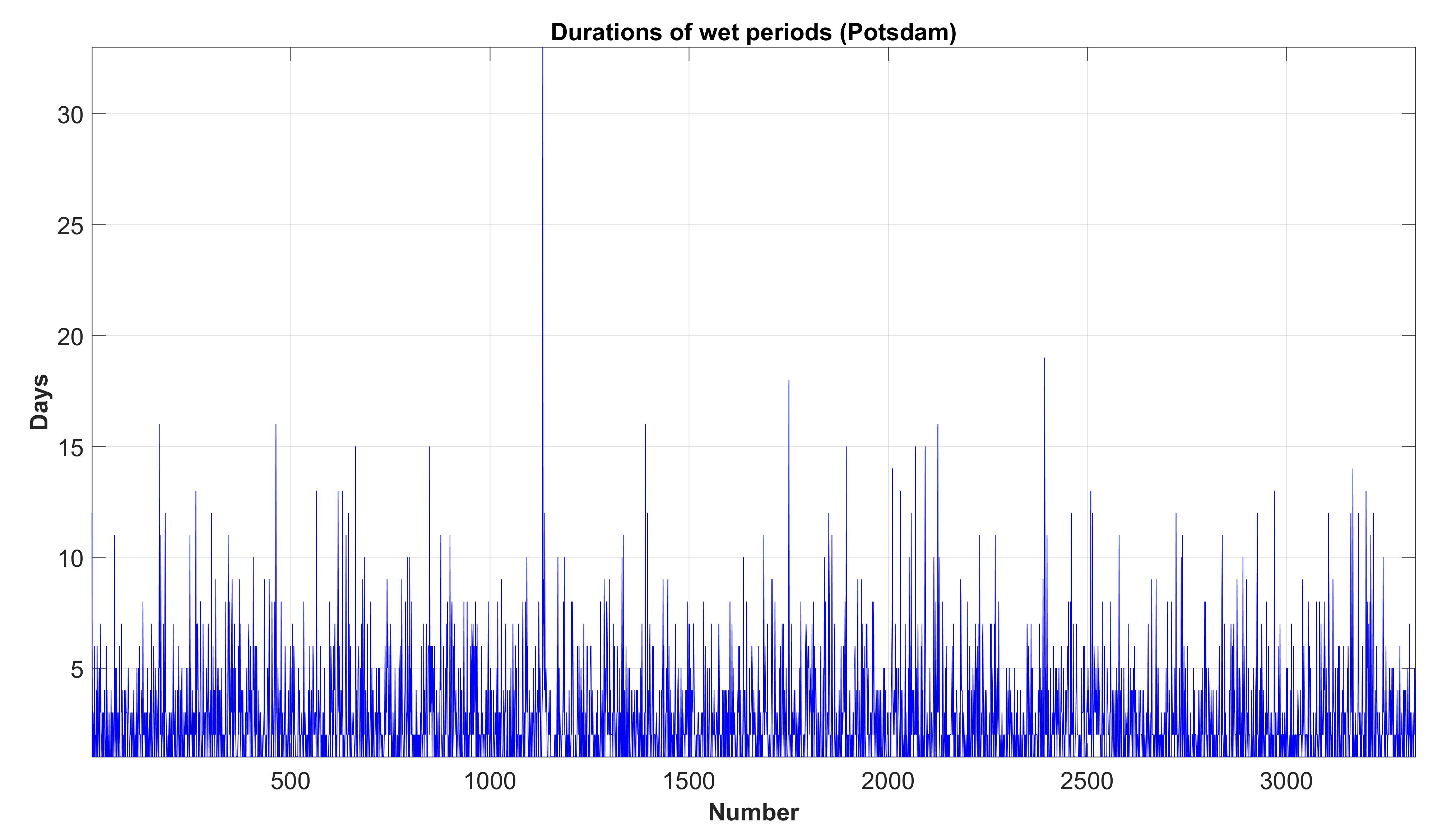
In order to analyze the statistical regularities of the duration of wet periods this data was rearranged as shown on Figures 2a and 2b.

a)

b)

Fig. 2: The durations of wet periods in Elista (a) and Potsdam (b).

On these figures the horizontal axis is the number of successive wet periods. It should be mentioned that directly before and after each wet period there is at least one dry day, that is, successive wet periods are separated by dry periods. On the vertical axis there lie the durations of wet periods. In other words, the height of each “pin” on these figures is the length of the corresponding wet period measured in days and the corresponding point on the horizontal axis is the number of the wet period.

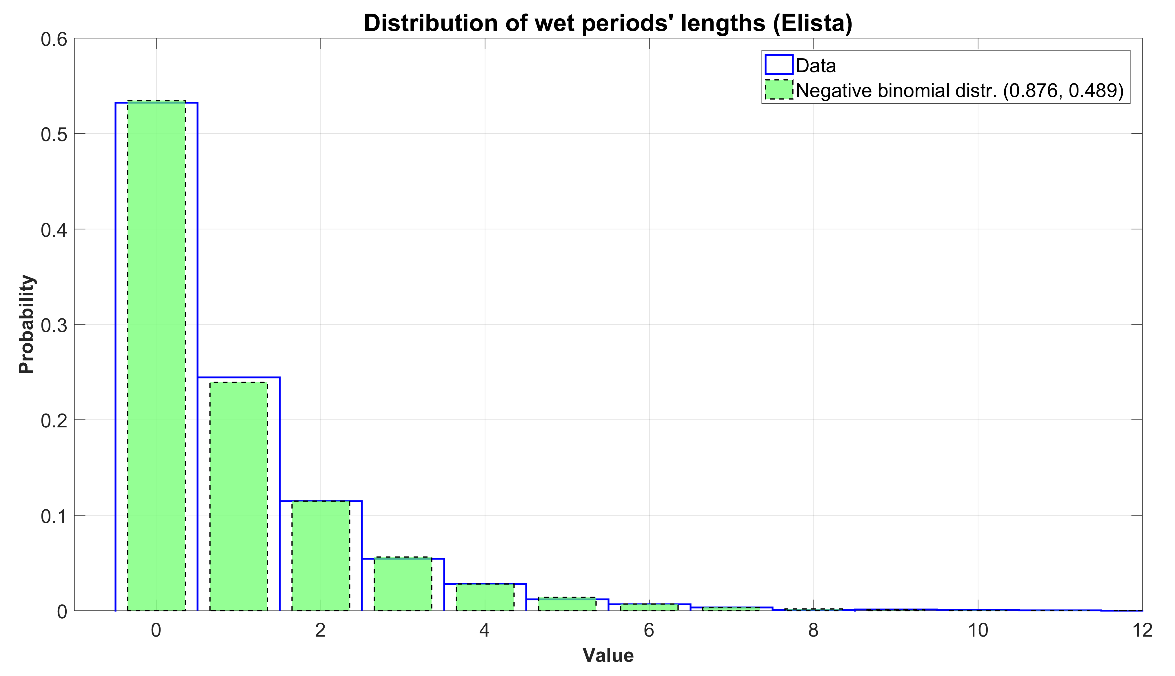
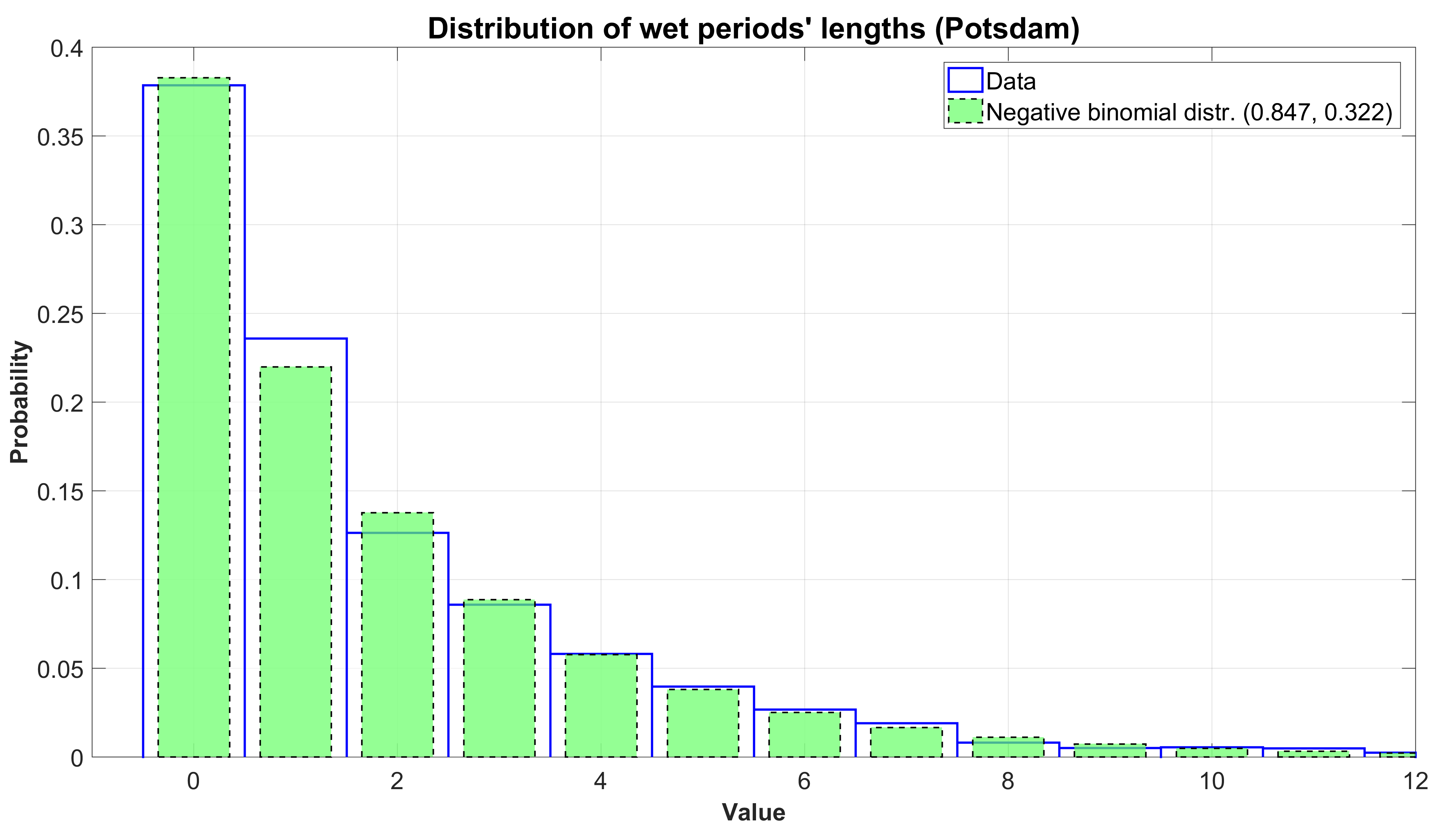
The samples of durations in both Elista and Potsdam were assumed homogeneous and independent. It was demonstrated that the fluctuations of the numbers of successive wet days with very high confidence fit the negative binomial distribution with shape parameter less than one (also see [3]). Figures 3a and 3b show the histograms constructed from the corresponding samples of duration periods and the fitted negative binomial distribution. In both cases the shape parameter $r$ turned out to be less than one. For Elista $r=0.876$, $p=0.489$, for Potsdam $r=0.847$, $p=0.322$.

a)

b)

Fig. 3: The histogram of durations of wet periods in Elista (a) and Potsdam (b) and the fitted negative binomial distribution.

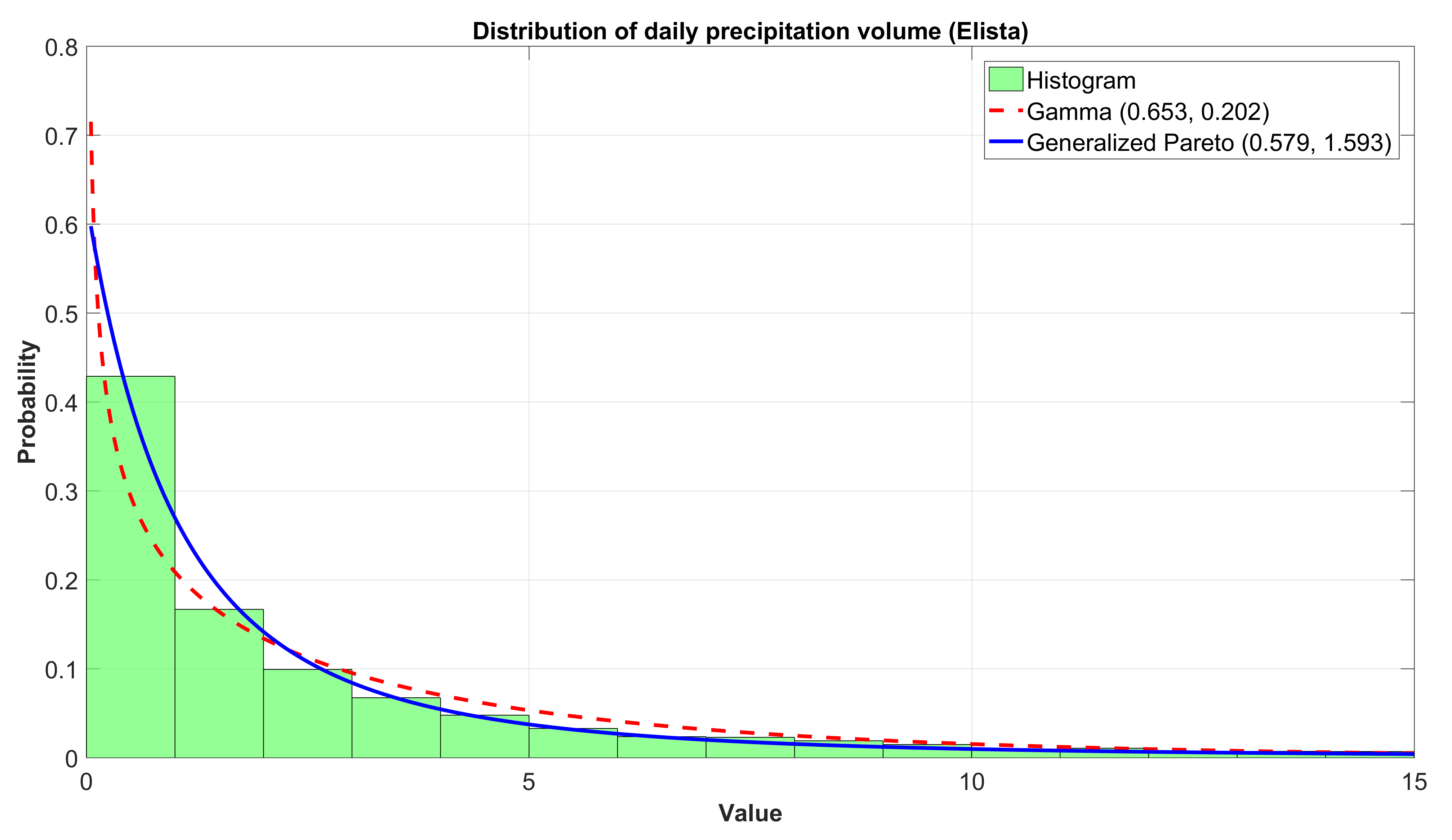
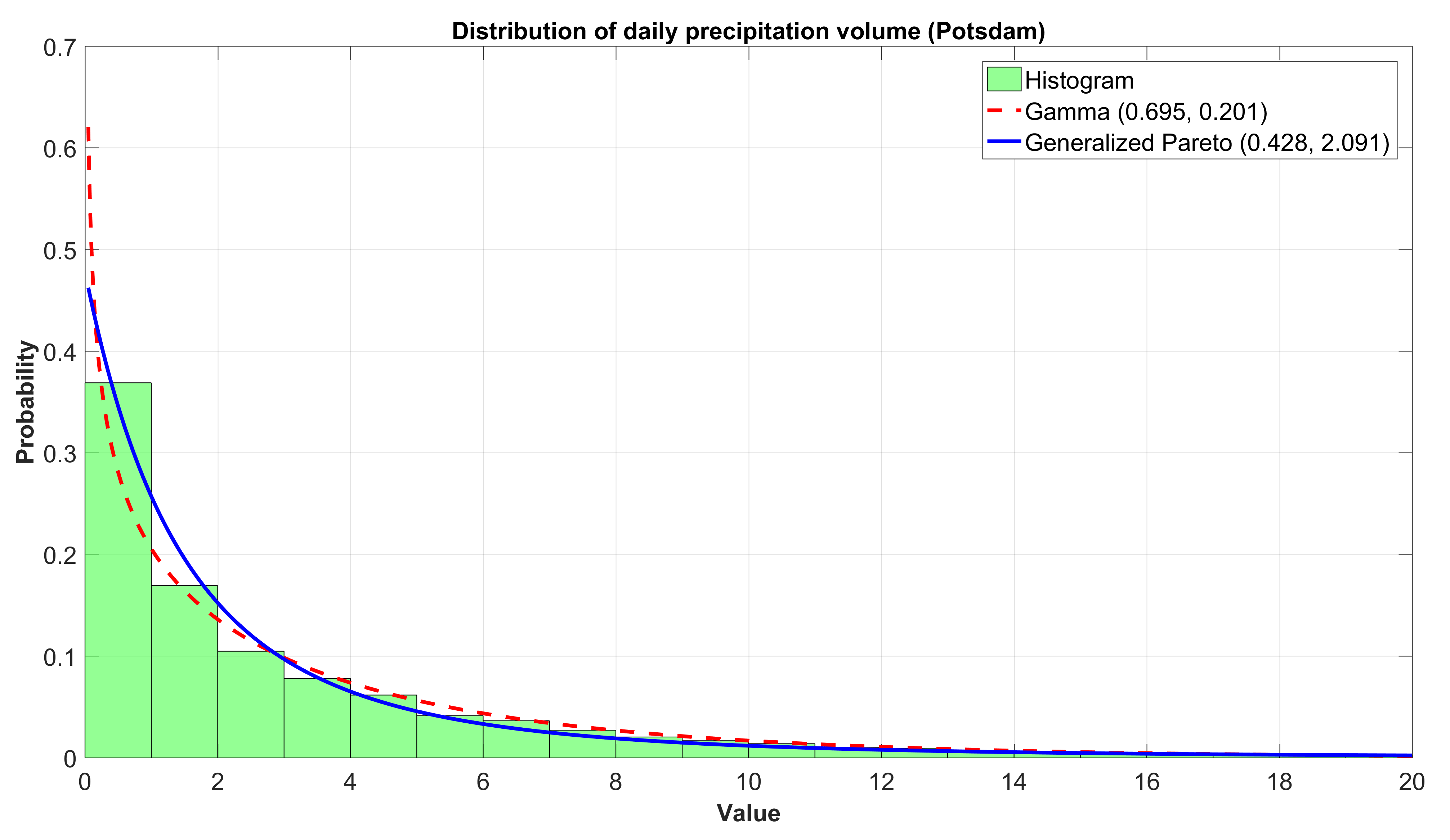
It is worth noting that at the same time the statistical analysis convincingly suggests the Pareto-type model for the distribution of daily precipitation volumes, see Figures 4a and 4b. For comparison, on these figures there are also presented the graphs of the best gamma-densities which, nevertheless, fit the histograms in a noticeably worse way than the Pareto distributions.

a)

b)

Fig. 4: The histogram of daily precipitation volumes in Elista (a) and Potsdam (b) and the fitted Pareto and gamma distributions.

In the same paper a schematic attempt was undertaken to explain this phenomenon by the fact that negative binomial distributions can be represented as mixed Poisson laws with mixing gamma-distributions. As is known, the Poisson distribution is the best model for the discrete stochastic chaos [4] by virtue of the universal principle of non-decrease of entropy in closed systems (see, e. g., [5, 6]) and the mixing distribution accumulates the statistical regularities in the influence of stochastic factors that can be assumed exogenous with respect to the local system under consideration.

In the paper [7] this explanation of the adequacy of the negative binomial model was concretized. For this purpose, the concept of a mixed geometric distribution introduced in [8] (also see [9, 10]) was used. In [7] it was demonstrated that any negative binomial distribution with shape parameter no greater than one is a mixed geometric distribution (this result is reproduced below as Theorem 1). Thereby, a “discrete” analog of a theorem due to L. Gleser [11] was proved. Gleser’s theorem establishes that a gamma distribution with shape parameter no greater than one can be represented as a mixed exponential distribution.

The representation of a negative binomial distribution as a mixed geometric law can be interpreted in terms of the Bernoulli trials as follows. First, as a result of some “preliminary” experiment the value of some random variables (r.v:s) taking values in $[0,1]$ is determined which is then used as the probability of success in the sequence of Bernoulli trials in which the original “unconditional” r.v. with the negative binomial distribution is nothing else than the “conditionally” geometrically distributed r.v. having the sense of the number of trials up to the first failure. This makes it possible to assume that the sequence of wet/dry days is not independent, but is conditionally independent and the random probability of success is determined by some outer stochastic factors. As such, we can consider the seasonality or the type of the cause of a rainy period.

The negative binomial model for the distribution of the duration of wet periods makes it possible to obtain asymptotic approximations for important characteristics of precipitation such as the distribution of the total precipitation volume per wet period and the distribution of the maximum daily precipitation volume within a wet period. The first of these approximations was proposed in [7], where an analog of the law of large numbers for negative binomial random sums was presented stating that the limit distribution for these sums is the gamma distribution.

The construction of the second approximation is the target of the present paper.

The paper is organized as follows. Definitions and notation are introduced in Section 2 which also contains some preliminary results providing some theoretical grounds for the negative binomial model of the probability distribution of the duration of wet periods. Main results are presented and proved in Section 3 where the asymptotic approximation is proposed for the distribution of the maximum daily precipitation volume within a wet period. Some analytic properties of the obtained limit distribution are described. In particular, it is demonstrated that under certain conditions the limit distribution is mixed exponential and hence, is infinitely divisible. It is shown that under the same conditions the limit distribution can be represented as a scale mixture of stable or Weibull or Pareto or folded normal laws. The corresponding product representations for the limit random variable can be used for its computer simulation. Several methods for the statistical estimation of the parameters of this distribution are proposed in Section 4. Section 5 contains the results of fitting the distribution proposed in Section 3 to real data by the methods described in Section 4.

2 Preliminaries

Although the main objects of our interest are the probability distributions, for convenience and brevity in what follows we will expound our results in terms of r.v:s with the corresponding distributions assuming that all the r.v:s under consideration are defined on one and the same probability space $(\Omega,\,\mathfrak{F},\,{\sf P})$.

In the paper, conventional notation is used. The symbols $\stackrel{{\scriptstyle d}}{{=}}$ and $\Longrightarrow$ denote the coincidence of distributions and convergence in distribution, respectively. The integer and fractional parts of a number $z$ will be respectively denoted $[z]$ and $\{z\}$.

A r.v. having the gamma distribution with shape parameter $r>0$ and scale parameter $\lambda>0$ will be denoted $G_{r,\lambda}$,

$${\sf P}(G_{r,\lambda}<x)=\int_{0}^{x}g(z;r,\lambda)dz,\ \ \text{with}\ \ g(x;r,\lambda)=\frac{\lambda^{r}}{\Gamma(r)}x^{r-1}e^{-\lambda x},\ x\geq 0,$$

where $\Gamma(r)$ is Euler’s gamma-function, $\Gamma(r)=\int_{0}^{\infty}x^{r-1}e^{-x}dx$, $r>0$.

In these notation, obviously, $G_{1,1}$ is a r.v. with the standard exponential distribution: ${\sf P}(G_{1,1}<x)=\big{[}1-e^{-x}\big{]}{\bf 1}(x\geq 0)$ (here and in what follows ${\bf 1}(A)$ is the indicator function of a set $A$).

The gamma distribution is a particular representative of the class of generalized gamma distributions (GG-distributions), which were first described in [12] as a special family of lifetime distributions containing both gamma distributions and Weibull distributions. A GG-distribution is the absolutely continuous distribution defined by the density

$$g^{*}(x;r,\gamma,\lambda)=\frac{|\gamma|\lambda^{r}}{\Gamma(r)}x^{\gamma r-1}e^{-\lambda x^{\gamma}},\ \ \ \ x\geq 0,$$

with $\gamma\in\mathbb{R}$, $\lambda>0$, $r>0$.

The properties of GG-distributions are described in [12, 13]. A r.v. with the density $g^{*}(x;r,\gamma,\lambda)$ will be denoted $G^{*}_{r,\gamma,\lambda}$. It can be easily made sure that

$$G^{*}_{r,\gamma,\lambda}\stackrel{{\scriptstyle d}}{{=}}G_{r,\lambda}^{1/\gamma}.$$ (1)

For a r.v. with the Weibull distribution, a particular case of GG-distributions corresponding to the density $g^{*}(x;1,\gamma,1)$ and the distribution function (d.f.) $\big{[}1-e^{-x^{\gamma}}\big{]}{\bf 1}(x\geq 0)$, we will use a special notation $W_{\gamma}$. Thus, $G_{1,1}\stackrel{{\scriptstyle d}}{{=}}W_{1}$. It is easy to see that

$$W_{1}^{1/\gamma}\stackrel{{\scriptstyle d}}{{=}}W_{\gamma}.$$ (2)

A r.v. with the standard normal d.f. $\Phi(x)$ will be denoted $X$,

$${\sf P}(X<x)=\Phi(x)=\frac{1}{\sqrt{2\pi}}\int_{-\infty}^{x}e^{-z^{2}/2}dz,\ \ \ \ x\in\mathbb{R}.$$

The distribution of the r.v. $|X|$, i. e. ${\sf P}(|X|<x)=2\Phi(x)-1$, $x\geq 0$, is called half-normal or folded normal.

The d.f. and the density of a strictly stable distribution with the characteristic exponent $\alpha$ and shape parameter $\theta$ defined by the characteristic function (ch.f.)

$$\mathfrak{f}_{\alpha,\theta}(t)=\exp\big{\{}-|t|^{\alpha}\exp\{-{\textstyle\frac{1}{2}}i\pi\theta\alpha\mathrm{sign}t\}\big{\}},\ \ \ \ t\in\mathbb{R},$$

wheter $0<\alpha\leq 2$, $|\theta|\leq\min\{1,\frac{2}{\alpha}-1\}$, will be respectively denoted $F_{\alpha,\theta}(x)$ and $f_{\alpha,\theta}(x)$ (see, e. g., [14]). A r.v. with the d.f. $F_{\alpha,\theta}(x)$ will be denoted $S_{\alpha,\theta}$.

To symmetric strictly stable distributions there correspond the value $\theta=0$ and the ch.f. $\mathfrak{f}_{\alpha,0}(t)=e^{-|t|^{\alpha}}$, $t\in\mathbb{R}$. To one-sided strictly stable distributions concentrated on the nonnegative halfline there correspond the values $\theta=1$ and $0<\alpha\leq 1$. The pairs $\alpha=1$, $\theta=\pm 1$ correspond to the distributions degenerate in $\pm 1$, respectively. All the rest strictly stable distributions are absolutely continuous. Stable densities cannot be explicitly represented via elementary functions with four exceptions: the normal distribution ($\alpha=2$, $\theta=0$), the Cauchy distribution ($\alpha=1$, $\theta=0$), the Lévy distribution ($\alpha=\frac{1}{2}$, $\theta=1$) and the distribution symmetric to the Lévy law ($\alpha=\frac{1}{2}$, $\theta=-1$).

It is well known that if $0<\alpha<2$, then ${\sf E}|S_{\alpha,\theta}|^{\beta}<\infty$ for any $\beta\in(0,\alpha)$, but the moments of the r.v. $S_{\alpha,\theta}$ of orders $\beta\geq\alpha$ do not exist (see, e. g., [14]). Despite the absence of explicit expressions for the densities of stable distributions in terms of elementary functions, it can be shown [16] that

$${\sf E}S_{\alpha,1}^{\beta}=\frac{\Gamma\big{(}1-\frac{\beta}{\alpha}\big{)}}{\Gamma(1-\beta)}$$ (3)

for $0<\beta<\alpha\leq 1$.

In [17, 18, 19] it was proved that if $\alpha\in(0,1)$ and the i.i.d. r.v:s $S_{\alpha,1}$ and $S^{\prime}_{\alpha,1}$ have the same strictly stable distribution, then the density $v_{\alpha}(x)$ of the r.v. $R_{\alpha}=S_{\alpha,1}/S^{\prime}_{\alpha,1}$ has the form

$$v_{\alpha}(x)=\frac{\sin(\pi\alpha)x^{\alpha-1}}{\pi[1+x^{2\alpha}+2x^{\alpha}\cos(\pi\alpha)]},\ \ \ x>0.$$ (4)

A r.v. $N_{r,p}$ is said to have the negative binomial distribution with parameters $r>0$ (“shape”) and $p\in(0,1)$ (“success probability”), if

$${\sf P}(N_{r,p}=k)=\frac{\Gamma(r+k)}{k!\Gamma(r)}\cdot p^{r}(1-p)^{k},\ \ \ \ k=0,1,2,...$$

A particular case of the negative binomial distribution corresponding to the value $r=1$ is the geometric distribution. Let $p\in(0,1)$ and let $N_{1,p}$ be the r.v. having the geometric distribution with parameter $p\,$:

$${\sf P}(N_{1,p}=k)=p(1-p)^{k},\ \ \ \ k=0,1,2,...$$

This means that for any $m\in\mathbb{N}$

$${\sf P}(N_{1,p}\geq m)=\sum\nolimits_{k=m}^{\infty}p(1-p)^{k}=(1-p)^{m}.$$

Let $Y$ be a r.v. taking values in the interval $(0,1)$. Moreover, let for all $p\in(0,1)$ the r.v. $Y$ and the geometrically distributed r.v. $N_{1,p}$ be independent. Let $V=N_{1,Y}$, that is, $V(\omega)=N_{1,Y(\omega)}(\omega)$ for any $\omega\in\Omega$. The distribution

$${\sf P}(V\geq m)=\int_{0}^{1}(1-y)^{m}d{\sf P}(Y<y),\ \ \ m\in\mathbb{N},$$

of the r.v. $V$ will be called $Y$-mixed geometric [8].

It is well known that the negative binomial distribution is a mixed Poisson distribution with the gamma mixing distribution [20] (also see [6]): for any $r>0$, $p\in(0,1)$ and $k\in\{0\}\bigcup\mathbb{N}$ we have

$$\frac{\Gamma(r+k)}{k!\Gamma(r)}\cdot p^{r}(1-p)^{k}=\frac{1}{k!}\int_{0}^{\infty}e^{-z}z^{k}g(z;r,\mu)dz,$$ (5)

where $\mu=p/(1-p)$.

Based on representation (5), in [7] it was proved that any negative binomial distribution with the shape parameter no greater than one is a mixed geometric distribution. Namely, the following statement was proved that gives an analytic explanation of the validity of the negative binomial model for the duration of wet periods measured in days (see the Introduction).

Theorem 1 [7]. The negative binomial distribution with parameters $r\in(0,1)$ and $p\in(0,1)$ is a mixed geometric distribution$:$ for any $k\in\{0\}\bigcup\mathbb{N}$

$$\frac{\Gamma(r+k)}{k!\Gamma(r)}\cdot p^{r}(1-p)^{k}=\int_{\mu}^{\infty}\Big{(}\frac{z}{z+1}\Big{)}\Big{(}1-\frac{z}{z+1}\Big{)}^{k}p(z;r,\mu)dz=\int_{p}^{1}y(1-y)^{k}h(y;r,p)dy,$$

where $\mu=p/(1-p)$ and the probability densities $p(z;r,\mu)$ and $h(y;r,p)$ have the forms

$$p(z;r,\mu)=\frac{\mu^{r}}{\Gamma(1-r)\Gamma(r)}\cdot\frac{\mathbf{1}(z\geq\mu)}{(z-\mu)^{r}z},$$

$$h(y;r,p)=\frac{p^{r}}{\Gamma(1-r)\Gamma(r)}\cdot\frac{(1-y)^{r-1}\mathbf{1}(p<y<1)}{y(y-p)^{r}}.$$

Furthermore, if $G_{r,\,1}$ and $G_{1-r,\,1}$ are independent gamma-distributed r.v:s, $\mu>0$, $p\in(0,1)$, then the density $p(z;r,\mu)$ corresponds to the r.v.

$$Z_{r,\mu}=\frac{\mu(G_{r,\,1}+G_{1-r,\,1})}{G_{r,\,1}}$$ (6)

and the density $h(y;r,p)$ corresponds to the r.v.

$$Y_{r,p}=\frac{p(G_{r,\,1}+G_{1-r,\,1})}{G_{r,\,1}+pG_{1-r,\,1}}.$$

Let $P(t)$, $t\geq 0$, be the standard Poisson process (homogeneous Poisson process with unit intensity). Then distribution (5) corresponds to the r.v. $N_{r,p}=P(G_{r,p/(1-p)})$, where the r.v. $G_{r,p/(1-p)}$ is independent of the process $P(t)$.

3 The probability distribution of extremal precipitation

In this section we will deduce the probability distribution of extremal daily precipitation within a wet period.

Let $r>0$, $\lambda>0$, $q\in(0,1)$, $n\in\mathbb{N}$, $p_{n}=\min\{q,\,\lambda/n\}$. It is easy to make sure that

$$n^{-1}G_{r,p_{n}/(1-p_{n})}\Longrightarrow G_{r,\lambda}$$ (7)

as $n\to\infty$.

Lemma 1. Let $\Lambda_{1},\Lambda_{2},\ldots$ be a sequence of positive r.v$:$s such that for any $n\in\mathbb{N}$ the r.v. $\Lambda_{n}$ is independent of the Poisson process $P(t)$, $t\geq 0$. The convergence

$$n^{-1}P(\Lambda_{n})\Longrightarrow\Lambda$$

as $n\to\infty$ to some nonnegative r.v. $\Lambda$ takes place if and only if

$$n^{-1}\Lambda_{n}\Longrightarrow\Lambda$$ (8)

as $n\to\infty$.

Proof. This statement is a particular case of Lemma 2 in [21] (also see Theorem 7.9.1 in [6]).

Consider a sequence of independent identically distributed (i.i.d.) r.v:s $X_{1},X_{2},\ldots$. Let $N_{1},N_{2},\ldots$ be a sequence of natural-valued r.v:s such that for each $n\in\mathbb{N}$ the r.v. $N_{n}$ is independent of the sequence $X_{1},X_{2},\ldots$. Denote $M_{n}=\max\{X_{1},\ldots,X_{N_{n}}\}$.

Let $F(x)$ be a d.f., $a\in\mathbb{R}$. Denote $\mathrm{rext}(F)=\sup\{x:\,F(x)<1\}$, $F^{-1}(a)=\inf\{x:\,F(x)\geq a\}$.

Lemma 2. Let $\Lambda_{1},\Lambda_{2},\ldots$ be a sequence of positive r.v$:$s such that for each $n\in\mathbb{N}$ the r.v. $\Lambda_{n}$ is independent of the Poisson process $P(t)$, $t\geq 0$. Let $N_{n}=P(\Lambda_{n})$. Assume that there exists a nonnegative r.v. $\Lambda$ such that convergence (8) takes place. Let $X_{1},X_{2},\ldots$ be i.i.d. r.v$:$s with a common d.f. $F(x)$. Assume also that $\mathrm{rext}(F)=\infty$ and there exists a number $\gamma>0$ such that for each $x>0$

$$\lim_{y\to\infty}\frac{1-F(xy)}{1-F(y)}=x^{-\gamma}.$$ (9)

Then

$$\lim_{n\to\infty}\sup_{x\geq 0}\bigg{|}{\sf P}\bigg{(}\frac{M_{n}}{F^{-1}(1-\frac{1}{n})}<x\bigg{)}-\int_{0}^{\infty}e^{-zx^{-\gamma}}d{\sf P}(\Lambda<z)\bigg{|}=0.$$

Proof. This statement is a particular case of Theorem 3.1 in [22].

Theorem 2. Let $n\in\mathbb{N}$, $\lambda>0$, $q\in(0,1)$ and let $N_{r,p_{n}}$ be a r.v. with the negative binomial distribution with parameters $r>0$ and $p_{n}=\min\{q,\lambda/n\}$. Let $X_{1},X_{2},\ldots$ be i.i.d. r.v$:$s with a common d.f. $F(x)$. Assume that $\mathrm{rext}(F)=\infty$ and there exists a number $\gamma>0$ such that relation (9) holds for any $x>0$. Then

$$\lim_{n\to\infty}\sup_{x\geq 0}\bigg{|}{\sf P}\bigg{(}\frac{\max\{X_{1},\ldots,X_{N_{r,p_{n}}}\}}{F^{-1}(1-\frac{1}{n})}<x\bigg{)}-F(x;r,\lambda,\gamma)\bigg{|}=0,$$

where

$$F(x;r,\lambda,\gamma)=\bigg{(}\frac{\lambda x^{\gamma}}{1+\lambda x^{\gamma}}\bigg{)}^{r},\ \ \ x\geq 0.$$

Proof. From (5) it follows that $N_{r,p_{n}}\stackrel{{\scriptstyle d}}{{=}}P(G_{r,p_{n}/(1-p_{n})}$. Therefore, from (7), Lemma 1 with $\Lambda_{n}=G_{r,p_{n}/(1-p_{n})}$ and Lemma 2 with the account of the absolute continuity of the limit distribution it immediately follows that

$$\lim_{n\to\infty}\sup_{x\geq 0}\bigg{|}{\sf P}\bigg{(}\frac{\max\{X_{1},\ldots,X_{N_{r,p_{n}}}\}}{F^{-1}(1-\frac{1}{n})}<x\bigg{)}-\frac{\lambda^{r}}{\Gamma(r)}\int_{0}^{\infty}e^{-z(\lambda+x^{-\gamma})}z^{r-1}dz\bigg{|}=0.$$

By elementary calculation it can be made sure that

$$\frac{\lambda^{r}}{\Gamma(r)}\int_{0}^{\infty}e^{-z(\lambda+x^{-\gamma})}z^{r-1}dz=\frac{\lambda^{r}}{\Gamma(r)(\lambda+x^{-\gamma})^{r}}\int_{0}^{\infty}e^{-z}z^{r-1}dz=\bigg{(}\frac{\lambda x^{\gamma}}{1+\lambda x^{\gamma}}\bigg{)}^{r}.$$

The theorem is proved.

It is worth noting that the limit distribution with the power-type decrease of the tail was obtained in Theorem 2 as a scale mixture of the Fréchet distribution (the type II extreme value distribution) in which the mixing law is the gamma distribution.

Since the Fréchet d.f. $e^{-x^{-\gamma}}$ with $\gamma>0$ corresponds to the r.v. $W_{\gamma}^{-1}$, it is easy to make sure that the d.f. $F(x;r,\lambda,\gamma)$ corresponds to the r.v. $M_{r,\gamma,\lambda}\equiv G_{r,\lambda}^{1/\gamma}W_{\gamma}^{-1}$, where the multipliers on the right-hand side are independent. From (1) and (2) it follows that

$$M_{r,\gamma,\lambda}\stackrel{{\scriptstyle d}}{{=}}\Big{(}\frac{G_{r,\lambda}}{W_{1}}\Big{)}^{1/\gamma}\stackrel{{\scriptstyle d}}{{=}}\frac{G^{*}_{r,\gamma,\lambda}}{W_{\gamma}}$$ (10)

where in each term the multipliers are independent. Consider the r.v. $G_{r,\lambda}/W_{1}$ in (10) in more detail. We have

$$\frac{G_{r,\lambda}}{W_{1}}\stackrel{{\scriptstyle d}}{{=}}\frac{G_{r,\lambda}}{G_{1,1}}\stackrel{{\scriptstyle d}}{{=}}\frac{G_{r,1}}{\lambda G_{1,1}}\stackrel{{\scriptstyle d}}{{=}}\frac{Q_{r,1}}{\lambda r},$$

where $Q_{r,1}$ is the r.v. having the Snedecor–Fisher distribution with parameters $r,\,1$ (‘degrees of freedom’) defined by the Lebesgue density

$$f_{r,1}(x)=\frac{r^{r+1}x^{r-1}}{(1+rx)^{r+1}},\ \ \ x\geq 0,$$

(see, e. g., [15], Section 27).

So,

$$M_{r,\gamma,\lambda}\stackrel{{\scriptstyle d}}{{=}}\Big{(}\frac{Q_{r,1}}{\lambda r}\Big{)}^{1/\gamma},$$ (11)

and the statement of theorem 2 can be re-formulated as

$$\frac{\max\{X_{1},\ldots,X_{N_{r,p_{n}}}\}}{F^{-1}(1-\frac{1}{n})}\Longrightarrow M_{r,\gamma,\lambda}\equiv\frac{G_{r,\lambda}^{1/\gamma}}{W_{\gamma}}\stackrel{{\scriptstyle d}}{{=}}\Big{(}\frac{Q_{r,1}}{\lambda r}\Big{)}^{1/\gamma}\ \ \ \ (n\to\infty).$$ (12)

The density of the limit distribution $F(x;r,\gamma,\lambda)$ of the extreme daily precipitation within a wet period has the form

$$p(x;r,\gamma,\lambda)=\frac{r\gamma\lambda^{r}x^{\gamma r-1}}{(1+\lambda x^{\gamma})^{r+1}}=\frac{\gamma r\lambda^{r}}{x^{1+\gamma}(\lambda+x^{-\gamma})^{r+1}},\ \ \ x>0.$$ (13)

It is easy to see that $p(x;r,\gamma,\lambda)=O(x^{-1-\gamma})$ as $x\to\infty$. Therefore ${\sf E}M_{r,\gamma,\lambda}^{\delta}<\infty$ only if $\delta<\gamma$. Moreover, from (12) it is possible to deduce explicit expressions for the moments of the r.v. $M_{r,\gamma,\lambda}$.

Theorem 3. Let $0<\delta<\gamma<\infty$. Then

$${\sf E}M_{r,\gamma,\lambda}^{\delta}=\frac{\Gamma\big{(}r+\frac{\delta}{\gamma}\big{)}\Gamma\big{(}1-\frac{\delta}{\gamma}\big{)}}{\lambda^{\delta/\gamma}\Gamma(r)}.$$

Proof. From (12) it follows that

$${\sf E}M_{r,\gamma,\lambda}^{\delta}={\sf E}G_{r,\lambda}^{\delta/\gamma}\cdot{\sf E}W_{1}^{-\delta/\gamma}.$$ (14)

It is easy to verify that

$${\sf E}G_{r,\lambda}^{\delta/\gamma}=\frac{\Gamma\big{(}r+\frac{\delta}{\gamma}\big{)}}{\lambda^{\delta/\gamma}\Gamma(r)},\ \ \ {\sf E}W_{1}^{-\delta/\gamma}=\Gamma\big{(}1-{\textstyle\frac{\delta}{\gamma}}\big{)}.$$ (15)

Hence follows the desired result.

To analyze the properties of the limit distribution in theorem 2 more thoroughly we will require some additional auxiliary results.

Lemma 3 [16]. Let $\gamma\in(0,1]$. Then

$$W_{\gamma}\stackrel{{\scriptstyle d}}{{=}}\frac{W_{1}}{S_{\gamma,1}}$$

with the r.v:s on the right-hand side being independent.

Lemma 4 [7]. Let $r\in(0,1]$, $\gamma\in(0,1]$, $\lambda>0$. Then

$$G_{r,\lambda}^{1/\gamma}\stackrel{{\scriptstyle d}}{{=}}G^{*}_{r,\gamma,\lambda}\stackrel{{\scriptstyle d}}{{=}}\frac{W_{\gamma}}{Z_{r,\lambda}^{1/\gamma}}\stackrel{{\scriptstyle d}}{{=}}\frac{W_{1}}{S_{\gamma,1}Z_{r,\lambda}^{1/\gamma}},$$

where the r.v. $Z_{r,\lambda}$ was defined in (6) and all the involved r.v$:$s are independent.

Theorem 4. Let $r\in(0,1]$, $\gamma\in(0,1]$, $\lambda>0$. Then the following product representations are valid$:$

$$M_{r,\gamma,\lambda}\stackrel{{\scriptstyle d}}{{=}}\frac{G_{r,\lambda}^{1/\gamma}S_{\gamma,1}}{W_{1}},$$ (16)

$$M_{r,\gamma,\lambda}\stackrel{{\scriptstyle d}}{{=}}\frac{W_{\gamma}}{W^{\prime}_{\gamma}}\cdot\frac{1}{Z_{r,\lambda}^{1/\gamma}}\stackrel{{\scriptstyle d}}{{=}}W_{1}\cdot\frac{R_{\gamma}}{W^{\prime}_{1}Z_{r,\lambda}^{1/\gamma}}\stackrel{{\scriptstyle d}}{{=}}\frac{\Pi R_{\gamma}}{Z_{r,\lambda}^{1/\gamma}}\stackrel{{\scriptstyle d}}{{=}}\frac{|X|\sqrt{2W_{1}}R_{\gamma}}{W^{\prime}_{1}Z_{r,\lambda}^{1/\gamma}},$$ (17)

where $W_{\gamma}\stackrel{{\scriptstyle d}}{{=}}W^{\prime}_{\gamma}$, $W_{1}\stackrel{{\scriptstyle d}}{{=}}W^{\prime}_{1}$, the r.v. $R_{\gamma}$ has the density (4), the r.v. $\Pi$ has the Pareto distribution$:$ ${\sf P}(\Pi>x)=(x+1)^{-1}$, $x\geq 0$, and in each term the involved r.v$:$s are independent.

Proof. Relation (16) follows from (12) and Lemma 3, relation (17) follows from (12) and Lemma 4 with the account of the representation $W_{1}\stackrel{{\scriptstyle d}}{{=}}|X|\sqrt{2W_{1}}$, the proof of which can be found in, say, [16].

With the account of the relation $R_{\gamma}\stackrel{{\scriptstyle d}}{{=}}R_{\gamma}^{-1}$, from (17) we obtain the following statement.

Corollary 1. Let $r\in(0,1]$, $\gamma\in(0,1]$, $\lambda>0$. Then the d.f. $F(x;r,\gamma,\lambda)$ is mixed exponential$:$

$$1-F(x;r,\gamma,\lambda)=\int_{0}^{\infty}e^{-ux}dA(u),\ \ \ x\geq 0,$$

where

$$A(u)={\sf P}\big{(}W_{1}R_{\gamma}Z_{r,\lambda}^{1/\gamma}<u\big{)},\ \ \ u\geq 0,$$

and all the involved r.v$:$s are independent.

Remark 1. It is worth noting that the mixing distribution in Corollary 1 is mixed exponential itself.

Corollary 2. Let $r\in(0,1]$, $\gamma\in(0,1]$, $\lambda>0$. Then the d.f. $F(x;r,\gamma,\lambda)$ is infinitely divisible.

Proof. This statement immediately follows from Corollary 1 and the result of Goldie [23] stating that the product of two independent non-negative random variables is infinitely divisible, if one of the two is exponentially distributed.

Theorem 3 states that the limit distribution in Theorem 2 can be represented as a scale mixture of exponential or stable or Weibull or Pareto or folded normal laws. The corresponding product representations for the r.v. $M_{r,\gamma,\lambda}$ can be used for its computer simulation.

In practice, the asymptotic approximation $F(x;r,\lambda,\gamma)$ for the distribution of the extreme daily precipitation within a wet period proposed by Theorem 2 is adequate, if the “success probability” is small enough, that is, if on the average the wet periods are long enough.

4 Estimation of the parameters $r$, $\lambda$ and $\gamma$

From (13) it can be seen that the realization of the maximum likelihood method for the estimation of the parameters $r$, $\lambda$ and $\gamma$ inevitably assumes the necessity of numerical solution of a system of transcendental equations by iterative procedures without any guarantee that the resulting maximum is global. The closeness of the initial approximation to the true maximum likelihood point in the three-dimensional parameter set might give a hope that the terminal extreme point found by the numerical algorithm is global.

For rough estimation of the parameters, the following considerably simpler method can be used. The resulting rough estimates can be used as a starting point for the ‘full’ maximum likelihood algorithm mentioned above in order to ensure the closeness of the initial approximation to the true solution. The rough method is based on that the quantiles of the d.f. $F(x;r,\lambda,\gamma)$ can be written out explicitly. Namely, the quantile $x(\epsilon;r,\lambda,\gamma)$ of the d.f. $F(x;r,\lambda,\gamma)$ of order $\epsilon\in(0,1)$, that is, the solution of the equation $F(x;r,\lambda,\gamma)=\epsilon$ with respect to $x$, obviously has the form

$$x(\epsilon;r,\lambda,\gamma)=\bigg{(}\frac{\epsilon^{1/r}}{\lambda-\lambda\epsilon^{1/r}}\bigg{)}^{1/\gamma}.$$

Let at our disposal there be observations $\{X_{i,j}\}$, $i=1,\ldots,m$, $j=1,\ldots,m_{i}$, where $i$ is the number of a wet period (the number of a sequence of rainy days), $j$ is the number of a day in the wet sequence, $m_{i}$ is the length of the $i$th wet sequence (the number of rainy days in the $i$th wet period), $m$ is the total number of wet sequences, $X_{i,j}$ is the precipitation volume on the $j$th day of the $i$th wet sequence. Construct the sample $X^{*}_{1},\ldots,X^{*}_{m}$ as

$$X^{*}_{k}=\max\{X_{k,1},\ldots,X_{k,m_{k}}\},\ \ \ k=1,\ldots,m.$$ (18)

Let $X^{*}_{(1)},\ldots,X^{*}_{(m)}$ be order statistics constructed from the sample $X^{*}_{1},\ldots,X^{*}_{m}$. Since we have three unknown parameters $r$, $\lambda$ and $\gamma$, fix three numbers $0<p_{1}<p_{2}<p_{3}<1$ and construct the system of equations

$${\displaystyle X^{*}_{([mp_{k}])}=\bigg{(}\frac{p_{k}^{1/r}}{\lambda-\lambda p_{k}^{1/r}}\bigg{)}^{1/\gamma}},\ \ \ k=1,2,3$$

(here the symbol $[a]$ denotes the integer part of a number $a$).

This system can be solved by standard techniques. For example, first, the number $s\equiv\frac{1}{r}$ can be found numerically as the solution of the equation

$$Cs=\log\frac{1-p_{3}^{s}}{1-p_{1}^{s}}\log\frac{X^{*}_{([mp_{1}])}}{X^{*}_{([mp_{2}])}}-\log\frac{1-p_{2}^{s}}{1-p_{1}^{s}}\log\frac{X^{*}_{([mp_{1}])}}{X^{*}_{([mp_{3}])}},$$

where

$$C=\log\frac{X^{*}_{([mp_{1}])}}{X^{*}_{([mp_{3}])}}\log\frac{p_{1}}{p_{2}}-\log\frac{X^{*}_{([mp_{1}])}}{X^{*}_{([mp_{2}])}}\log\frac{p_{1}}{p_{3}}.$$

Having obtained the value of $s$, one can then find the values of $\gamma$ and $\lambda$ explicitly:

$$\gamma=\frac{s(\log p_{1}-\log p_{3})+\log(1-p_{3}^{s})-\log(1-p_{1}^{s})}{\log X^{*}_{([mp_{1}])}-\log X^{*}_{([mp_{3}])}},$$ (19)

$$\lambda=\frac{p_{2}^{s}}{(1-p_{2}^{s})(X^{*}_{([mp_{2}])})^{\gamma}}.$$ (20)

As $p_{1}$, $p_{2}$ and $p_{3}$ one may take, say, $p_{k}=\frac{k}{4}$, $k=1,2,3$. Or it is possible to fix a $\tau\in(0,\frac{1}{4})$, set $p_{1}=\tau$, $p_{2}=\frac{1}{2}$, $p_{3}=1-\tau$ and choose a $\tau$ that provides the best fit of the estimated model d.f. $F(x;r,\lambda,\gamma)$ with the empirical d.f.

If the parameter $r$ is known (for example, it is estimated beforehand while solving the problem of fitting the negative binomial distribution to the empirical data on the lengths of wet periods), then the parameters $\lambda$ and $\gamma$ can be estimated directly by formulas (19) and (20).

With known $r$, the more accurate estimates of the parameters $\lambda$ and $\gamma$ can be also found by minimizing the discrepancy between the empirical and model d.f:s by the least squares techniques. Namely, from the Glivenko theorem it follows that

$$\bigg{(}\frac{\lambda(X^{*}_{(i)})^{\gamma}}{1+\lambda(X^{*}_{(i)})^{\gamma}}\bigg{)}^{r}\approx\frac{i}{m}.$$ (21)

As this is so, for every $i=1,\ldots,m-1$ the following implications take place:

$$\eqref{7}\Longleftrightarrow\Big{\{}\frac{\lambda(X^{*}_{(i)})^{\gamma}}{1+\lambda(X^{*}_{(i)})^{\gamma}}\approx\Big{(}\frac{i}{m}\Big{)}^{1/r}\Big{\}}\Longleftrightarrow\Big{\{}\frac{1}{1+\lambda(X^{*}_{(i)})^{\gamma}}\approx 1-\Big{(}\frac{i}{m}\Big{)}^{1/r}\Big{\}}\Longleftrightarrow$$

$$\Longleftrightarrow\Big{\{}\lambda(X^{*}_{(i)})^{\gamma}\approx\frac{i^{1/r}}{m^{1/r}-i^{1/r}}\Big{\}}\Longleftrightarrow\Big{\{}\log\lambda+\gamma\log X^{*}_{(i)}\approx\log\frac{i^{1/r}}{m^{1/r}-i^{1/r}}\Big{\}}.$$

Therefore the estimates $\widehat{\lambda}$ and $\widehat{\gamma}$ of the parameters $\lambda$ and $\gamma$ can be found as the solution of the least squares problem

$$(\log\widehat{\lambda},\,\widehat{\gamma})=\mathrm{arg}\min_{\log\lambda,\gamma}\sum_{i=1}^{m-1}\big{(}\log\lambda+\gamma\log X^{*}_{(i)}-c_{i}\big{)}^{2},$$

where

$$c_{i}=\log\frac{i^{1/r}}{m^{1/r}-i^{1/r}}.$$

This solution can be written out explicitly so that finally we have

$$\widehat{\gamma}=\frac{(m-1)\sum_{i=1}^{m-1}c_{i}\log X^{*}_{(i)}-\sum_{i=1}^{m-1}\log X^{*}_{(i)}\sum_{i=1}^{m-1}c_{i}}{(m-1)\sum_{i=1}^{m-1}(\log X^{*}_{(i)})^{2}-(\sum_{i=1}^{m-1}\log X^{*}_{(i)})^{2}},$$ (22)

$$\widehat{\lambda}=\exp\Big{\{}\frac{1}{m-1}\Big{(}\sum\nolimits_{i=1}^{m-1}c_{i}-\widehat{\gamma}\sum\nolimits_{i=1}^{m-1}\log X^{*}_{(i)}\Big{)}\Big{\}}.$$ (23)

5 The statistical analysis of real data

In this section we present the results of statistical estimation of the distribution of extremal daily precipitation within a wet period by the methods described in the preceding section. As the data, we use the observations of daily precipitation in Potsdam and Elista from $1950$ to $2009$.

First of all, notice that the Pareto distribution of daily precipitation volumes (see Figure 4) satisfies condition (9). Therefore, the asymptotic approximation provided by Theorem 2 can be applied to the statistical analysis of the real data.

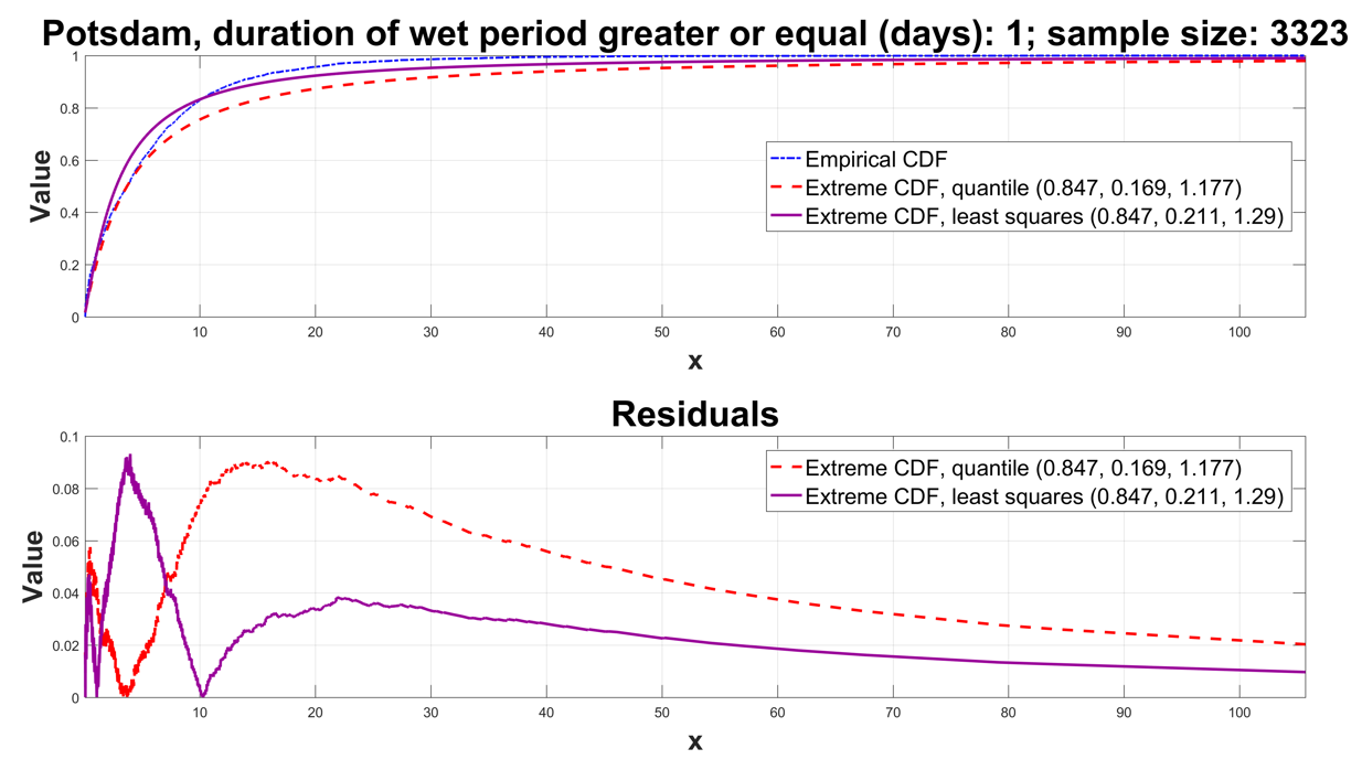
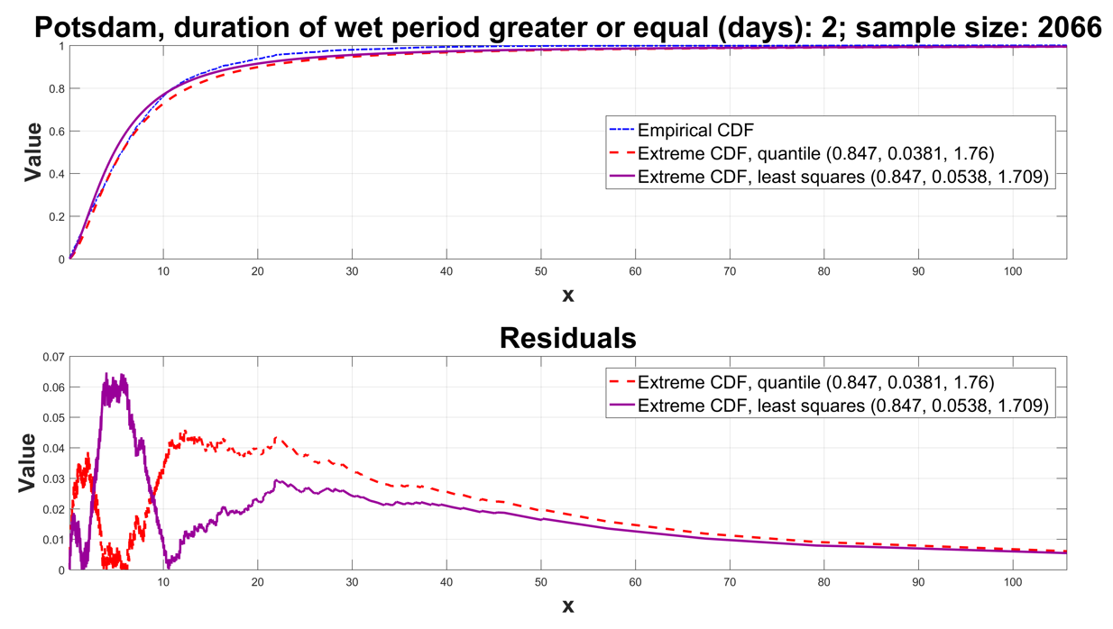
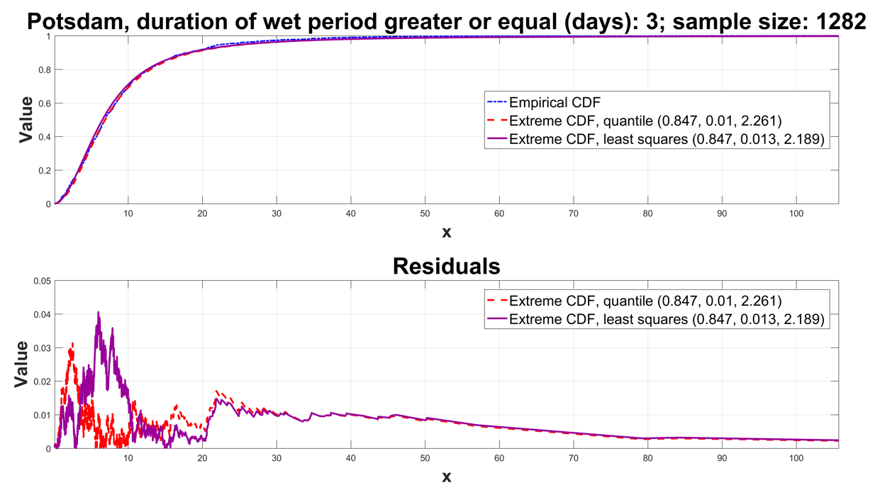
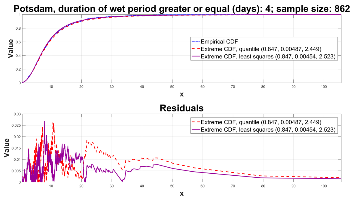
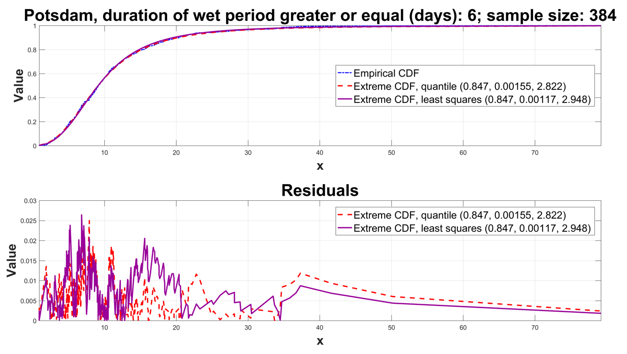
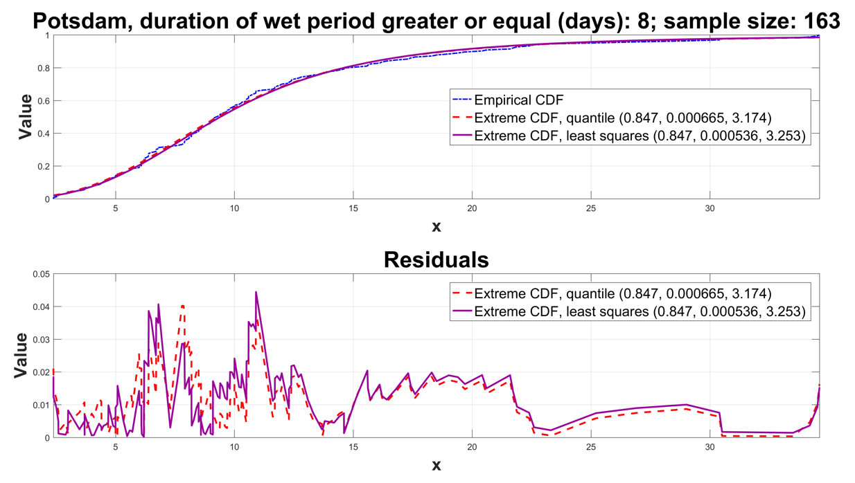
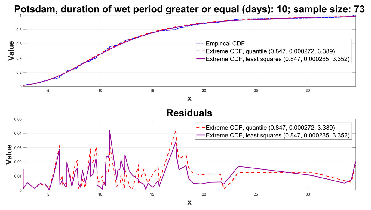
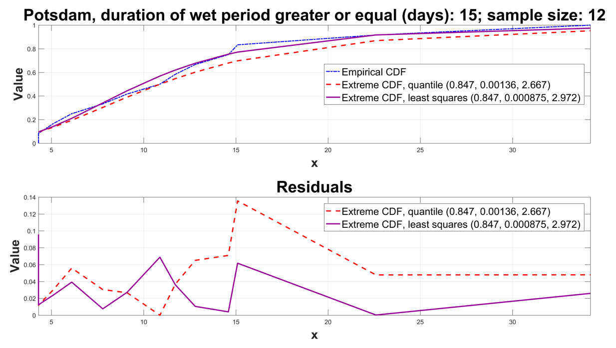
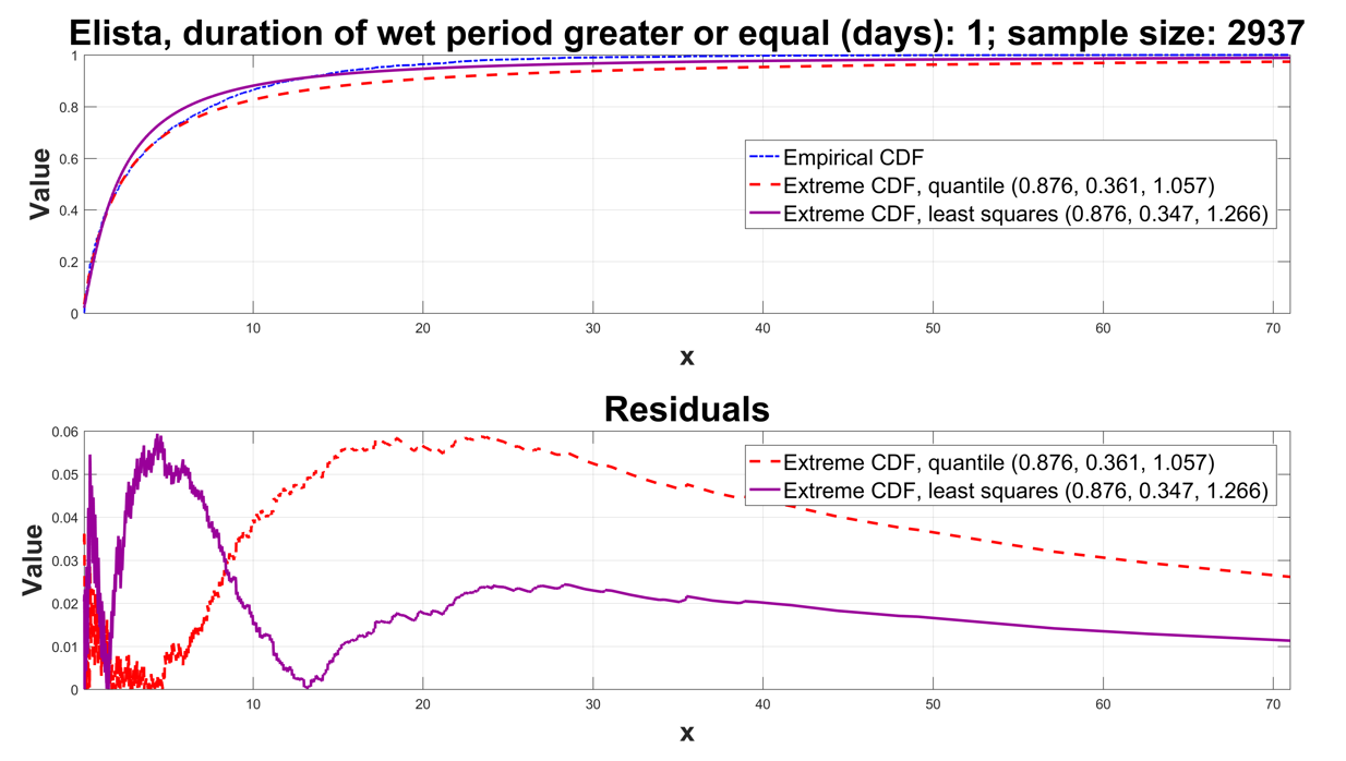
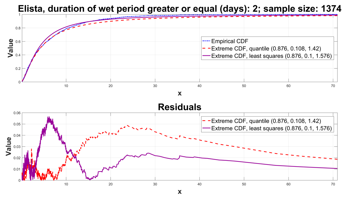
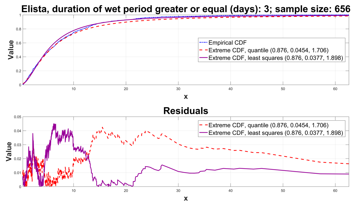
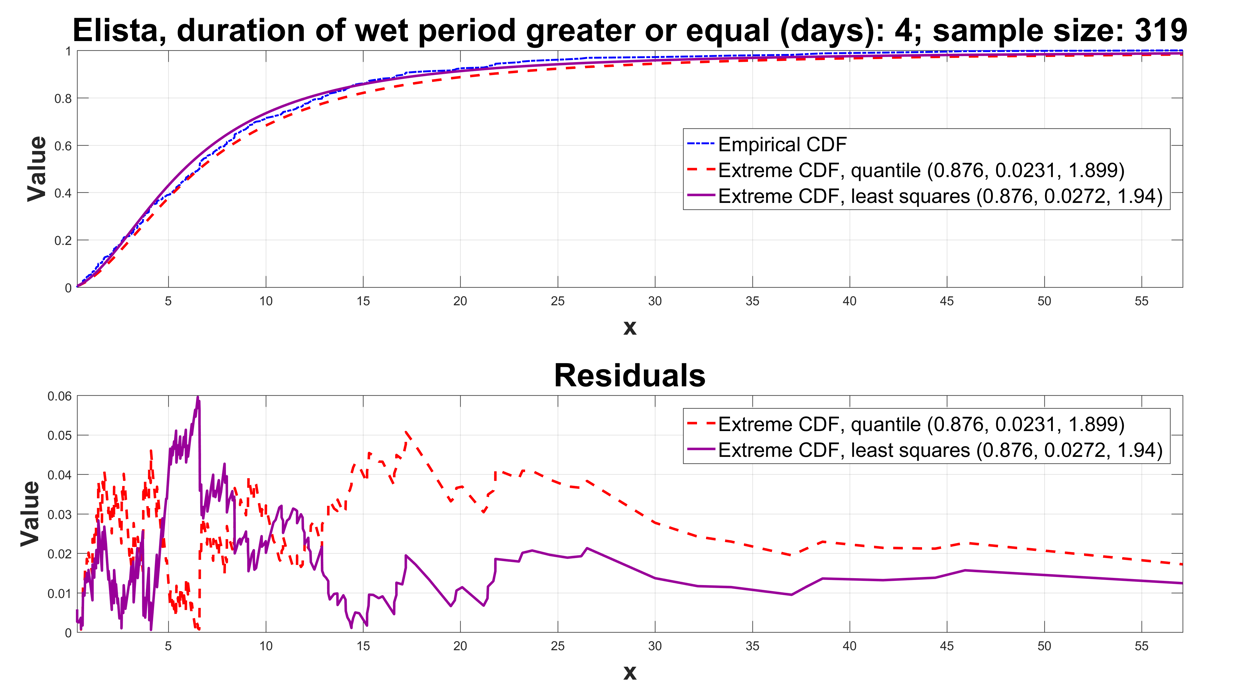
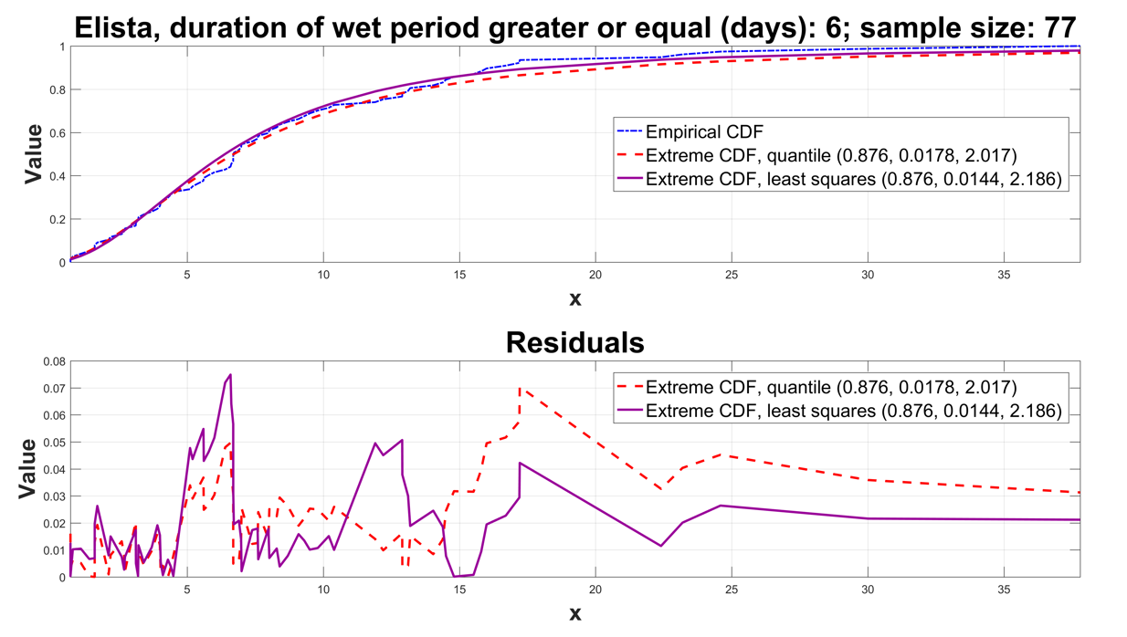
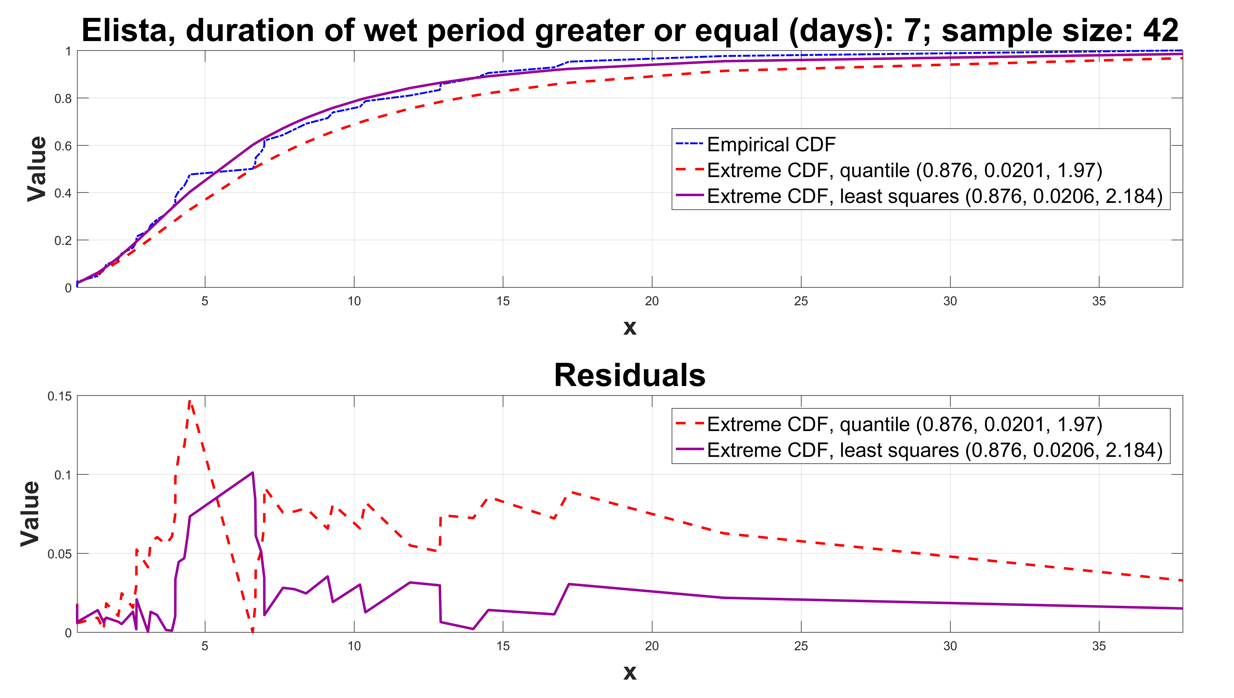
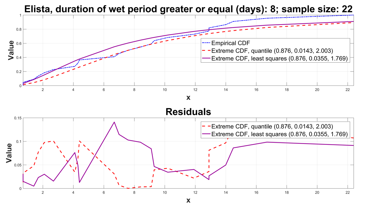
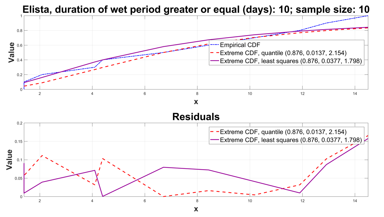
The parameter $r$ is assumed known and its value coincides with that of the negative binomial distribution (see the Introduction): $r=0.847$ for Potsdam and $r=0.876$ for Elista. Figures 5 and 6 illustrate the approximation of the empirical d.f. by the model d.f. $F(x;r,\gamma,\lambda)$ with $\gamma$ and $\lambda$ estimated by the ‘rough’ formulas (19) and (20) as well as by the least squares formulas (22) and (23). To illustrate the asymptotic character of the approximation $F(x;r,\gamma,\lambda)$ we consider a sort of censoring in which the censoring threshold is the minimum length of the wet periods which varies from 1 day (full sample) to 15 days.

For each censoring threshold $h=\min_{i}m_{i}$ the sample is formed according to the rule (18).

For each value of the threshold on the upper graph there are

• the empirical d.f. (dot-dash line);

• the d.f. $F(x;,r,\gamma,\lambda)$ with $\gamma$ and $\lambda$ estimated by the ‘rough’ formulas (19) and (20) (dash line);

• the d.f. $F(x;,r,\gamma,\lambda)$ with $\gamma$ and $\lambda$ estimated by the least squares formulas (22) and (23) (continuous line).

On the lower graph there is the discrepancy (the uniform distance) between the empirical d.f. and the fitted model d.f. The types of lines correspond to those on the upper graph.

First of all, from Figures 5 and 6 it is seen that the asymptotic model $F(x;r,\gamma,\lambda)$ provides very good approximation to the real statistical regularities in the behavior of extremal daily precipitation within a wet period. As this is so, the least squares formulas (22) and (23) yield more accurate estimates for the parameters of the model d.f.

It should be also noted that these figures illustrate the dependence of the accuracy of the approximation on the censoring threshold and the censored sample size. The approximation is satisfactory even if the censoring threshold $h$ is greater or equal to three and the censored sample size is grater than 150. As this is so, the influence of the threshold $h$ on the accuracy is more noticeable than that of the sample size.

a)

b)

c)

d)

e)

f)

g)

h)

Fig. 5: Empirical and estimated model extreme precipitation distributions (Potsdam). Duration of wet period is no less than: a) 1; b) 2; c) 3; d) 4; e) 6; f) 8; g) 10; h) 15 days.

a)

b)

c)

d)

e)

f)

g)

h)

Fig. 6: Empirical and estimated model extreme precipitation distributions (Elista). Duration of wet period is no less than: a) 1; b) 2; c) 3; d) 4; e) 6; f) 7; g) 8; h) 10 days.

References

- [1] Zolina O., Simmer C., Belyaev K., Gulev S., Koltermann P. Changes in the duration of European wet and dry spells during the last 60 years // Journal of Climate, 2013. Vol. 26. P. 2022–2047.
- [2] Korolev V. Yu., Gorshenin A. K., Gulev S. K., Belyaev K. P., Grusho A. A. Statistical Analysis of Precipitation Events // AIP Conference Proceedings, 2017. Also available on arXiv:1705.11055 [math.PR]
- [3] Gorhenin A. K. On some mathematical and program methods for the construction of structure models of information flows // Informatics and Its Applications, 2017. Vol. 11. No. 1. P. 58–68.
- [4] Kingman J. F. C. Poisson processes. – Oxford: Clarendon Press, 1993.
- [5] Gnedenko B. V., Korolev V. Yu. Random Summation: Limit Theorems and Applications. – Boca Raton: CRC Press, 1996.
- [6] Korolev V. Yu., Bening V. E., Shorgin S. Ya. Mathematical Foundations of Risk Theory. 2nd Edition. – Moscow: FIZMATLIT, 2011.
- [7] Korolev V. Yu. Analogs of the Gleser theorem for negative binomial and generalized gamma distributions and some their applications // Informatics and Its Applications, 2017. Vol. 11. No. 3.
- [8] Korolev V. Yu. Limit distributions for doubly stochastically rarefied renewal processes and their properties // Theory Probab. Appl., 2016. Vol. 61. No. 4. P. 753–773.
- [9] Korolev V. Yu., Korchagin A. Yu., Zeifman A. I. Poisson theorem for the scheme of Bernoulli trials with random probability of success and a discrete analog of the Weibull distribution // Informatics and Its Applications, 2016. Vol. 10. No. 4. P. 11–20.
- [10] Korolev V. Yu., Korchagin A. Yu., Zeifman A. I. On doubly stochastic rarefaction of renewal processes // AIP Conference Proceedings, 2017.
- [11] Gleser L. J. The gamma distribution as a mixture of exponential distributions // American Statistician, 1989. Vol. 43. P. 115–117.
- [12] Stacy E. W. A generalization of the gamma distribution // Annals of Mathematical Statistics, 1962. Vol. 33. P. 1187–1192.
- [13] Zaks L. M., Korolev V. Yu. Generalized variance gamma distributions as limit laws for random sums // Informatics and Its Applications, 2013. Vol. 7. No. 1. P. 105–115.
- [14] Zolotarev V. M. One-Dimensional Stable Distributions. – Providence, R.I.: American Mathematical Society, 1986.
- [15] Johnson, N. L., Kotz S., Balakrishnan N. Continuous Univariate Distributions, Vol. 2 (2nd Edition). – New York: Wiley, 1995.
- [16] Korolev V. Yu. Product representations for random variables with the Weibull distributions and their applications // Journal of Mathematical Sciences, 2016. Vol. 218. No. 3. P. 298–313.
- [17] Kotz S., Ostrovskii I. V. A mixture representation of the Linnik distribution // Statistics and Probability Letters, 1996. Vol. 26. P. 61–64.
- [18] Korolev V. Yu., Zeifman A. I. A note on mixture representations for the Linnik and Mittag-Leffler distributions and their applications // Journal of Mathematical Sciences, 2017. Vol. 218. No. 3. P. 314–327.
- [19] Korolev V. Yu., Zeifman A. I. Convergence of statistics constructed from samples with random sizes to the Linnik and Mittag-Leffler distributions and their generalizations // Journal of Korean Statistical Society. Available online 25 July 2016. Also available on arXiv:1602.02480v1 [math.PR].
- [20] Greenwood M., Yule G. U. An inquiry into the nature of frequency-distributions of multiple happenings, etc. // J. Roy. Statist. Soc., 1920. Vol. 83. P. 255–279.
- [21] Korolev V. Yu. On convergence of distributions of compound Cox processes to stable laws // Theory of Probability and its Applications, 1999. Vol. 43. Vol. 4. P. 644–650.
- [22] Korolev V. Yu., Sokolov I. A. Mathematical Models of Inhomogeneous Flows of Extremal Events. – Moscow: Torus-Press, 2008.
- [23] Goldie C. M. A class of infinitely divisible distributions // Math. Proc. Cambridge Philos. Soc., 1967. Vol. 63. P. 1141-1143.