Accuracy First: Selecting a Differential Privacy Level for Accuracy-Constrained ERM

Katrina Ligett Caltech and Hebrew University Seth Neel University of Pennsylvania Aaron Roth University of Pennsylvania Bo Waggoner University of Pennsylvania Z. Steven Wu University of Pennsylvania
(May 2017)
Abstract

Traditional approaches to differential privacy assume a fixed privacy requirement ε𝜀\varepsilon for a computation, and attempt to maximize the accuracy of the computation subject to the privacy constraint. As differential privacy is increasingly deployed in practical settings, it may often be that there is instead a fixed accuracy requirement for a given computation and the data analyst would like to maximize the privacy of the computation subject to the accuracy constraint. This raises the question of how to find and run a maximally private empirical risk minimizer subject to a given accuracy requirement. We propose a general “noise reduction” framework that can apply to a variety of private empirical risk minimization (ERM) algorithms, using them to “search” the space of privacy levels to find the empirically strongest one that meets the accuracy constraint, incurring only logarithmic overhead in the number of privacy levels searched. The privacy analysis of our algorithm leads naturally to a version of differential privacy where the privacy parameters are dependent on the data, which we term ex-post privacy, and which is related to the recently introduced notion of privacy odometers. We also give an ex-post privacy analysis of the classical AboveThreshold privacy tool, modifying it to allow for queries chosen depending on the database. Finally, we apply our approach to two common objectives, regularized linear and logistic regression, and empirically compare our noise reduction methods to (i) inverting the theoretical utility guarantees of standard private ERM algorithms and (ii) a stronger, empirical baseline based on binary search.

1 Introduction and Related Work

Differential Privacy [6, 7] enjoys over a decade of study as a theoretical construct, and a much more recent set of large-scale practical deployments, including by Google [9] and Apple [10]. As the large theoretical literature is put into practice, we start to see disconnects between assumptions implicit in the theory and the practical necessities of applications. In this paper we focus our attention on one such assumption in the domain of private empirical risk minimization (ERM): that the data analyst first chooses a privacy requirement, and then attempts to obtain the best accuracy guarantee (or empirical performance) that she can, given the chosen privacy constraint. Existing theory is tailored to this view: the data analyst can pick her privacy parameter ε𝜀\varepsilon via some exogenous process, and either plug it into a “utility theorem” to upper bound her accuracy loss, or simply deploy her algorithm and (privately) evaluate its performance. There is a rich and substantial literature on private convex ERM that takes this approach, weaving tight connections between standard mechanisms in differential privacy and standard tools for empirical risk minimization. These methods for private ERM include output and objective perturbation [4, 13, 17, 3], covariance perturbation [18], the exponential mechanism [15, 2], and stochastic gradient descent [2, 20, 11, 5, 19].

While these existing algorithms take a privacy-first perspective, in practice, product requirements may impose hard accuracy constraints, and privacy (while desirable) may not be the over-riding concern. In such situations, things are reversed: the data analyst first fixes an accuracy requirement, and then would like to find the smallest privacy parameter consistent with the accuracy constraint. Here, we find a gap between theory and practice. The only theoretically sound method available is to take a “utility theorem” for an existing private ERM algorithm and solve for the smallest value of ε𝜀\varepsilon (the differential privacy parameter)—and other parameter values that need to be set—consistent with her accuracy requirement, and then run the private ERM algorithm with the resulting ε𝜀\varepsilon. But because utility theorems tend to be worst-case bounds, this approach will generally be extremely conservative, leading to a much larger value of ε𝜀\varepsilon (and hence a much larger leakage of information) than is necessary for the problem at hand. Alternately, the analyst could attempt an empirical search for the smallest value of ε𝜀\varepsilon consistent with her accuracy goals. However, because this search is itself a data-dependent computation, it incurs the overhead of additional privacy loss. Furthermore, it is not a priori clear how to undertake such a search with nontrivial privacy guarantees for two reasons: first, the worst case could involve a very long search which reveals a large amount of information, and second, the selected privacy parameter is now itself a data-dependent quantity, and so it is not sensible to claim a “standard” guarantee of differential privacy for any finite value of ε𝜀\varepsilon ex-ante.

In this paper, we describe, analyze, and empirically evaluate a principled variant of this second approach, which attempts to empirically find the smallest value of ε𝜀\varepsilon consistent with an accuracy requirement. We give a meta-method that can be applied to several interesting classes of private learning algorithms and introduces very little privacy overhead as a result of the privacy-parameter search. Conceptually, our meta-method initially computes a very private hypothesis, and then gradually subtracts noise (making the computation less and less private) until a sufficient level of accuracy is achieved. One key technique that saves significant factors in privacy loss over naive search is the use of correlated noise generated by the method of [14], which formalizes the conceptual idea of “subtracting” noise without incurring additional privacy overhead. In order to select the most private of these queries that meets the accuracy requirement, we introduce a natural modification of the now-classic AboveThreshold algorithm [7], which iteratively checks a sequence of queries on a dataset and privately releases the index of the first to approximately exceed some fixed threshold. Its privacy cost increases only logarithmically with the number of queries. We provide an analysis of AboveThreshold that holds even if the queries themselves are the result of differentially private computations, showing that if AboveThreshold terminates after t𝑡t queries, one only pays the privacy costs of AboveThreshold plus the privacy cost of revealing those first t𝑡t private queries. When combined with the above-mentioned correlated noise technique of [14], this gives an algorithm whose privacy loss is equal to that of the final hypothesis output – the previous ones coming “for free” – plus the privacy loss of AboveThreshold. Because the privacy guarantees achieved by this approach are not fixed a priori, but rather are a function of the data, we introduce and apply a new, corresponding privacy notion, which we term ex-post privacy, and which is closely related to the recently introduced notion of “privacy odometers” [16].

In Section 4, we empirically evaluate our noise reduction meta-method, which applies to any ERM technique which can be described as a post-processing of the Laplace mechanism. This includes both direct applications of the Laplace mechanism, like output perturbation [4]; and more sophisticated methods like covariance perturbation [18], which perturbs the covariance matrix of the data and then performs an optimization using the noisy data. Our experiments concentrate on 2subscript2\ell_{2} regularized least-squares regression and 2subscript2\ell_{2} regularized logistic regression, and we apply our noise reduction meta-method to both output perturbation and covariance perturbation. Our empirical results show that the active, ex-post privacy approach massively outperforms inverting the theory curve, and also improves on a baseline “ε𝜀\varepsilon-doubling” approach.

2 Privacy Background and Tools

2.1 Differential Privacy and Ex-Post Privacy

Let 𝒳𝒳\mathcal{X} denote the data domain. We call two datasets D,D𝒳𝐷superscript𝐷superscript𝒳D,D^{\prime}\in\mathcal{X}^{*} neighbors (written as DDsimilar-to𝐷superscript𝐷D\sim D^{\prime}) if D𝐷D can be derived from Dsuperscript𝐷D^{\prime} by replacing a single data point with some other element of 𝒳𝒳\mathcal{X}.

Definition 2.1 (Differential Privacy [6]).

Fix ε0𝜀0\varepsilon\geq 0. A randomized algorithm A:𝒳𝒪:𝐴superscript𝒳𝒪A:\mathcal{X}^{*}\rightarrow\mathcal{O} is ε𝜀\varepsilon-differentially private if for every pair of neighboring data sets DD𝒳similar-to𝐷superscript𝐷superscript𝒳D\sim D^{\prime}\in\mathcal{X}^{*}, and for every event S𝒪𝑆𝒪S\subseteq\mathcal{O}:

Pr[A(D)S]exp(ε)Pr[A(D)S].Pr𝐴𝐷𝑆𝜀Pr𝐴superscript𝐷𝑆\Pr[A(D)\in S]\leq\exp(\varepsilon)\Pr[A(D^{\prime})\in S].

We call exp(ε)𝜀\exp(\varepsilon) the privacy risk factor.

It is possible to design computations that do not satisfy the differential privacy definition, but whose outputs are private to an extent that can be quantified after the computation halts. For example, consider an experiment that repeatedly runs an εsuperscript𝜀\varepsilon^{\prime}-differentially private algorithm, until a stopping condition defined by the output of the algorithm itself is met. This experiment does not satisfy ε𝜀\varepsilon-differential privacy for any fixed value of ε𝜀\varepsilon, since there is no fixed maximum number of rounds for which the experiment will run (for a fixed number of rounds, a simple composition theorem, Theorem 2.5, shows that the ε𝜀\varepsilon-guarantees in a sequence of computations “add up.”) However, if ex-post we see that the experiment has stopped after k𝑘k rounds, the data can in some sense be assured an “ex-post privacy loss” of only kε𝑘superscript𝜀k\varepsilon^{\prime}. Rogers et al. [16] initiated the study of privacy odometers, which formalize this idea. Their goal was to develop a theory of privacy composition when the data analyst can choose the privacy parameters of subsequent computations as a function of the outcomes of previous computations.

We apply a related idea here, for a different purpose. Our goal is to design one-shot algorithms that always achieve a target accuracy but that may have variable privacy levels depending on their input.

Definition 2.2.

Given a randomized algorithm 𝒜:𝒳𝒪:𝒜superscript𝒳𝒪\operatorname*{\mathcal{A}}:\mathcal{X}^{*}\to\mathcal{O}, define the ex-post privacy loss111If 𝒜𝒜\operatorname*{\mathcal{A}}’s output is from a continuous distribution rather than discrete, we abuse notation and write Pr[𝒜(D)=o]Pr𝒜𝐷𝑜\Pr[\operatorname*{\mathcal{A}}(D)=o] to mean the probability density at output o𝑜o. of 𝒜𝒜\operatorname*{\mathcal{A}} on outcome o𝑜o to be

Loss(o)=maxD,D:DDlogPr[𝒜(D)=o]Pr[𝒜(D)=o].\text{Loss(}{o})=\max_{D,D^{\prime}:D\sim D^{\prime}}\log\frac{\Pr\left[\operatorname*{\mathcal{A}}(D)=o\right]}{\Pr\left[\operatorname*{\mathcal{A}}(D^{\prime})=o\right]}.

We refer to exp(Loss(o))\exp\left(\text{Loss(}{o})\right) as the ex-post privacy risk factor.

Definition 2.3 (Ex-Post Differential Privacy).

Let :𝒪(0{}):𝒪subscriptabsent0\mathcal{E}:\mathcal{O}\to(\mathbb{R}_{\geq 0}\cup\{\infty\}) be a function on the outcome space of algorithm 𝒜:𝒳𝒪:𝒜superscript𝒳𝒪\operatorname*{\mathcal{A}}:\mathcal{X}^{*}\to\mathcal{O}. Given an outcome o=A(D)𝑜𝐴𝐷o=A(D), we say that 𝒜𝒜\operatorname*{\mathcal{A}} satisfies (o)𝑜\mathcal{E}(o)-ex-post differential privacy if for all o𝒪𝑜𝒪o\in\mathcal{O}, Loss(o)(o)\text{Loss(}{o})\leq\mathcal{E}(o).

Note that if (o)ε𝑜𝜀\mathcal{E}(o)\leq\varepsilon for all o𝑜o, 𝒜𝒜\operatorname*{\mathcal{A}} is ε𝜀\varepsilon-differentially private. Ex-post differential privacy has the same semantics as differential privacy, once the output of the mechanism is known: it bounds the log-likelihood ratio of the dataset being D𝐷D vs. Dsuperscript𝐷D^{\prime}, which controls how an adversary with an arbitrary prior on the two cases can update her posterior.

2.2 Differential Privacy Tools

Differentially private computations enjoy two nice properties:

Theorem 2.4 (Post Processing [6]).

Let A:𝒳𝒪:𝐴superscript𝒳𝒪A:\mathcal{X}^{*}\rightarrow\mathcal{O} be any ε𝜀\varepsilon-differentially private algorithm, and let f:𝒪𝒪:𝑓𝒪superscript𝒪f:\mathcal{O}\rightarrow\mathcal{O^{\prime}} be any function. Then the algorithm fA:𝒳𝒪:𝑓𝐴superscript𝒳superscript𝒪f\circ A:\mathcal{X}^{*}\rightarrow\mathcal{O}^{\prime} is also ε𝜀\varepsilon-differentially private.

Post-processing implies that, for example, every decision process based on the output of a differentially private algorithm is also differentially private.

Theorem 2.5 (Composition [6]).

Let A1:𝒳𝒪:subscript𝐴1superscript𝒳𝒪A_{1}:\mathcal{X}^{*}\rightarrow\mathcal{O}, A2:𝒳𝒪:subscript𝐴2superscript𝒳superscript𝒪A_{2}:\mathcal{X}^{*}\rightarrow\mathcal{O}^{\prime} be algorithms that are ε1subscript𝜀1\varepsilon_{1}- and ε2subscript𝜀2\varepsilon_{2}-differentially private, respectively. Then the algorithm A:𝒳𝒪×𝒪:𝐴superscript𝒳𝒪superscript𝒪A:\mathcal{X}^{*}\rightarrow\mathcal{O}\times\mathcal{O^{\prime}} defined as A(x)=(A1(x),A2(x))𝐴𝑥subscript𝐴1𝑥subscript𝐴2𝑥A(x)=(A_{1}(x),A_{2}(x)) is (ε1+ε2)subscript𝜀1subscript𝜀2(\varepsilon_{1}+\varepsilon_{2})-differentially private.

The composition theorem holds even if the composition is adaptive—-see [8] for details.

The Laplace mechanism. The most basic subroutine we will use is the Laplace mechanism. The Laplace Distribution centered at 00 with scale b𝑏b is the distribution with probability density function Lap(z|b)=12be|z|bLapconditional𝑧𝑏12𝑏superscript𝑒𝑧𝑏\text{Lap}\left({z|b}\right)=\frac{1}{2b}e^{-\frac{|z|}{b}}. We say XLap(b)similar-to𝑋Lap𝑏X\sim\text{Lap}\left({b}\right) when X𝑋X has Laplace distribution with scale b𝑏b. Let f:𝒳d:𝑓superscript𝒳superscript𝑑f\colon\mathcal{X}^{*}\rightarrow\mathbb{R}^{d} be an arbitrary d𝑑d-dimensional function. The 1subscript1\ell_{1} sensitivity of f𝑓f is defined to be Δ1(f)=maxDDf(D)f(D)1subscriptΔ1𝑓subscriptsimilar-to𝐷superscript𝐷subscriptnorm𝑓𝐷𝑓superscript𝐷1\Delta_{1}(f)=\max_{D\sim D^{\prime}}\|f(D)-f(D^{\prime})\|_{1}. The Laplace mechanism with parameter ε𝜀\varepsilon simply adds noise drawn independently from Lap(Δ1(f)ε)LapsubscriptΔ1𝑓𝜀\text{Lap}\left({\frac{\Delta_{1}(f)}{\varepsilon}}\right) to each coordinate of f(x)𝑓𝑥f(x).

Theorem 2.6 ([6]).

The Laplace mechanism is ε𝜀\varepsilon-differentially private.

Gradual private release. Koufogiannis et al. [14] study how to gradually release private data using the Laplace mechanism with an increasing sequence of ε𝜀\varepsilon values, with a privacy cost scaling only with the privacy of the marginal distribution on the least private release, rather than the sum of the privacy costs of independent releases. For intuition, the algorithm can be pictured as a continuous random walk starting at some private data v𝑣v with the property that the marginal distribution at each point in time is Laplace centered at v𝑣v, with variance increasing over time. Releasing the value of the random walk at a fixed point in time gives a certain output distribution, for example, v^^𝑣\hat{v}, with a certain privacy guarantee ε𝜀\varepsilon. To produce v^superscript^𝑣\hat{v}^{\prime} whose ex-ante distribution has higher variance (is more private), one can simply “fast forward” the random walk from a starting point of v^^𝑣\hat{v} to reach v^superscript^𝑣\hat{v}^{\prime}; to produce a less private v^superscript^𝑣\hat{v}^{\prime}, one can “rewind.” The total privacy cost is max{ε,ε}𝜀superscript𝜀\max\{\varepsilon,\varepsilon^{\prime}\} because, given the “least private” point (say v^^𝑣\hat{v}), all “more private” points can be derived as post-processings given by taking a random walk of a certain length starting at v^^𝑣\hat{v}. Note that were the Laplace random variables used for each release independent, the composition theorem would require summing the ε𝜀\varepsilon values of all releases.

In our private algorithms, we will use their noise reduction mechanism as a building block to generate a list of private hypotheses θ1,,θTsuperscript𝜃1superscript𝜃𝑇\theta^{1},\ldots,\theta^{T} with gradually increasing ε𝜀\varepsilon values. Importantly, releasing any prefix (θ1,,θt)superscript𝜃1superscript𝜃𝑡(\theta^{1},\ldots,\theta^{t}) only incurs the privacy loss in θtsuperscript𝜃𝑡\theta^{t}. More formally:

Algorithm 1 Noise Reduction [14]: NR(v,Δ,{εt})NR𝑣Δsubscript𝜀𝑡\textsc{NR}(v,\Delta,\{\varepsilon_{t}\})
Input: private vector v𝑣v, sensitivity parameter ΔΔ\Delta, list ε1<ε2<<εTsubscript𝜀1subscript𝜀2subscript𝜀𝑇\varepsilon_{1}<\varepsilon_{2}<\dots<\varepsilon_{T}
Set v^T:=v+Lap(Δ/εT)assignsubscript^𝑣𝑇𝑣LapΔsubscript𝜀𝑇\hat{v}_{T}:=v+\text{Lap}\left({\Delta/\varepsilon_{T}}\right) \triangleright drawn i.i.d. for each coordinate
for t=T1,T2,,1𝑡𝑇1𝑇21t=T-1,T-2,\dots,1 do
     With probability (εtεt+1)2superscriptsubscript𝜀𝑡subscript𝜀𝑡12\left(\frac{\varepsilon_{t}}{\varepsilon_{t+1}}\right)^{2}: set v^t:=v^t+1assignsubscript^𝑣𝑡subscript^𝑣𝑡1\hat{v}_{t}:=\hat{v}_{t+1}
     Else: set v^t:=v^t+1+Lap(Δ/εt)assignsubscript^𝑣𝑡subscript^𝑣𝑡1LapΔsubscript𝜀𝑡\hat{v}_{t}:=\hat{v}_{t+1}+\text{Lap}\left({\Delta/\varepsilon_{t}}\right) \triangleright drawn i.i.d. for each coordinate
Return v^1,,v^Tsubscript^𝑣1subscript^𝑣𝑇\hat{v}_{1},\dots,\hat{v}_{T}
Theorem 2.7 ([14]).

Let f𝑓f have 1subscript1\ell_{1} sensitivity ΔΔ\Delta and let v^1,,v^Tsubscript^𝑣1subscript^𝑣𝑇\hat{v}_{1},\dots,\hat{v}_{T} be the output of Algorithm 1 on v=f(D)𝑣𝑓𝐷v=f(D), ΔΔ\Delta, and the increasing list ε1,,εTsubscript𝜀1subscript𝜀𝑇\varepsilon_{1},\dots,\varepsilon_{T}. Then for any t𝑡t, the algorithm which outputs the prefix (v^1,,v^t)subscript^𝑣1subscript^𝑣𝑡(\hat{v}_{1},\dots,\hat{v}_{t}) is εtsubscript𝜀𝑡\varepsilon_{t}-differentially private.

2.3 AboveThreshold with Private Queries

Our high-level approach to our eventual ERM problem will be as follows: Generate a sequence of hypotheses θ1,,θTsubscript𝜃1subscript𝜃𝑇\theta_{1},\dots,\theta_{T}, each with increasing accuracy and decreasing privacy; then test their accuracy levels sequentially, outputting the first one whose accuracy is “good enough.” The classical AboveThreshold algorithm [7] takes in a dataset and a sequence of queries and privately outputs the index of the first query to exceed a given threshold (with some error due to noise). We would like to use AboveThreshold to perform these accuracy checks, but there is an important obstacle: for us, the “queries” themselves depend on the private data.222In fact, there are many applications beyond our own in which the sequence of queries input to AboveThreshold might be the result of some private prior computation on the data, and where we would like to release both the stopping index of AboveThreshold and the “query object.” (In our case, the query objects will be parameterized by learned hypotheses θ1,,θTsubscript𝜃1subscript𝜃𝑇\theta_{1},\dots,\theta_{T}.) A standard composition analysis would involve first privately publishing all the queries, then running AboveThreshold on these queries (which are now public). Intuitively, though, it would be much better to generate and publish the queries one at a time, until AboveThreshold halts, at which point one would not publish any more queries. The problem with analyzing this approach is that, a-priori, we do not know when AboveThreshold will terminate; to address this, we analyze the ex-post privacy guarantee of the algorithm.333This result does not follow from a straightforward application of privacy odometers from [16], because the privacy analysis of algorithms like the noise reduction technique is not compositional.

Algorithm 2 InteractiveAboveThreshold: IAT(D,ε,W,Δ,M)IAT𝐷𝜀𝑊Δ𝑀\textsc{IAT}(D,\varepsilon,W,\Delta,M)
Input: Dataset D𝐷D, privacy loss ε𝜀\varepsilon, threshold W𝑊W, 1subscript1\ell_{1} sensitivity ΔΔ\Delta, algorithm M𝑀M
Let W^=W+Lap(2Δε)^𝑊𝑊Lap2Δ𝜀\hat{W}=W+\text{Lap}\left({\frac{2\Delta}{\varepsilon}}\right)
for  each query t=1,,T𝑡1𝑇t=1,\dots,T do
     Query ftM(D)tsubscript𝑓𝑡𝑀subscript𝐷𝑡f_{t}\leftarrow M(D)_{t}
     if ft(D)+Lap(4Δε)W^subscript𝑓𝑡𝐷Lap4Δ𝜀^𝑊f_{t}(D)+\text{Lap}\left({\frac{4\Delta}{\varepsilon}}\right)\geq\hat{W}then Output (t𝑡t, ftsubscript𝑓𝑡f_{t}); Halt.      
Output (T𝑇T, perpendicular-to\perp).

Let us say that an algorithm M(D)=(f1,,fT)𝑀𝐷subscript𝑓1subscript𝑓𝑇M(D)=(f_{1},\ldots,f_{T}) is (ε1,,εT)\varepsilon_{1},\ldots,\varepsilon_{T})-prefix-private if for each t𝑡t, the function that runs M(D)𝑀𝐷M(D) and outputs just the prefix (f1,,ft)subscript𝑓1subscript𝑓𝑡(f_{1},\ldots,f_{t}) is εtsubscript𝜀𝑡\varepsilon_{t}-differentially private.

Lemma 2.8.

Let M:𝒳(𝒳𝒪)T:𝑀superscript𝒳superscriptsuperscript𝒳𝒪𝑇M:\mathcal{X}^{*}\rightarrow(\mathcal{X}^{*}\rightarrow\mathcal{O})^{T} be a (ε1,,εT)subscript𝜀1subscript𝜀𝑇(\varepsilon_{1},\ldots,\varepsilon_{T})-prefix private algorithm that returns T𝑇T queries, and let each query output by M𝑀M have 1subscript1\ell_{1} sensitivity at most ΔΔ\Delta. Then Algorithm 2 run on D𝐷D, εAsubscript𝜀𝐴\varepsilon_{A}, W𝑊W, ΔΔ\Delta, and M𝑀M is \mathcal{E}-ex-post differentially private for ((t,))=εA+εt𝑡subscript𝜀𝐴subscript𝜀𝑡\mathcal{E}((t,\cdot))=\varepsilon_{A}+\varepsilon_{t} for any t[T]𝑡delimited-[]𝑇t\in[T].

The proof, which is a variant on the proof of privacy for AboveThreshold [7], appears in the appendix, along with an accuracy theorem for IAT.

Remark 2.9.

Throughout we study ε𝜀\varepsilon-differential privacy, instead of the weaker (ε,δ)𝜀𝛿(\varepsilon,\delta) (approximate) differential privacy. Part of the reason is that an analogue of Lemma 2.8 does not seem to hold for (ε,δ)𝜀𝛿(\varepsilon,\delta)-differentially private queries without further assumptions, as the necessity to union-bound over the δ𝛿\delta “failure probability” that the privacy loss is bounded for each query can erase the ex-post gains. We leave obtaining similar results for approximate differential privacy as an open problem.

3 Noise-Reduction with Private ERM

In this section, we provide a general private ERM framework that allows us to approach the best privacy guarantee achievable on the data given a target excess risk goal. Throughout the section, we consider an input dataset D𝐷D that consists of n𝑛n row vectors X1,X2,,Xnpsubscript𝑋1subscript𝑋2subscript𝑋𝑛superscript𝑝X_{1},X_{2},\ldots,X_{n}\in\mathbb{R}^{p} and a column yn𝑦superscript𝑛y\in\mathbb{R}^{n}. We will assume that each Xi11subscriptnormsubscript𝑋𝑖11\|X_{i}\|_{1}\leq 1 and |yi|1subscript𝑦𝑖1|y_{i}|\leq 1. Let di=(Xi,yi)p+1subscript𝑑𝑖subscript𝑋𝑖subscript𝑦𝑖superscript𝑝1d_{i}=(X_{i},y_{i})\in\mathbb{R}^{p+1} be the i𝑖i-th data record. Let \ell be a loss function such that for any hypothesis θ𝜃\theta and any data point (Xi,yi)subscript𝑋𝑖subscript𝑦𝑖(X_{i},y_{i}) the loss is (θ,(Xi,yi))𝜃subscript𝑋𝑖subscript𝑦𝑖\ell(\theta,(X_{i},y_{i})). Given an input dataset D𝐷D and a regularization parameter λ𝜆\lambda, the goal is to minimize the following regularized empirical loss function over some feasible set C𝐶C:

L(θ,D)=1ni=1n(θ,(Xi,yi))+λ2θ22.𝐿𝜃𝐷1𝑛superscriptsubscript𝑖1𝑛𝜃subscript𝑋𝑖subscript𝑦𝑖𝜆2superscriptsubscriptnorm𝜃22L(\theta,D)=\frac{1}{n}\sum_{i=1}^{n}\ell(\theta,(X_{i},y_{i}))+\frac{\lambda}{2}\|\theta\|_{2}^{2}.

Let θ=argminθC(θ,D)superscript𝜃subscriptargmin𝜃𝐶𝜃𝐷\theta^{*}=\operatorname*{\mathrm{argmin}}_{\theta\in C}\ell(\theta,D). Given a target accuracy parameter α𝛼\alpha, we wish to privately compute a θpsubscript𝜃𝑝\theta_{p} that satisfies L(θp,D)L(θ,D)+α𝐿subscript𝜃𝑝𝐷𝐿superscript𝜃𝐷𝛼L(\theta_{p},D)\leq L(\theta^{*},D)+\alpha, while achieving the best ex-post privacy guarantee. For simplicity, we will sometimes write L(θ)𝐿𝜃L(\theta) for L(θ,D)𝐿𝜃𝐷L(\theta,D).

One simple baseline approach is a “doubling method”: Start with a small ε𝜀\varepsilon value, run an ε𝜀\varepsilon-differentially private algorithm to compute a hypothesis θ𝜃\theta and use the Laplace mechanism to estimate the excess risk of θ𝜃\theta; if the excess risk is lower than the target, output θ𝜃\theta; otherwise double the value of ε𝜀\varepsilon and repeat the same process. (See the appendix for details.) As a result, we pay for privacy loss for every hypothesis we compute and every excess risk we estimate.

In comparison, our meta-method provides a more cost-effective way to select the privacy level. The algorithm takes a more refined set of privacy levels ε1<<εTsubscript𝜀1subscript𝜀𝑇\varepsilon_{1}<\ldots<\varepsilon_{T} as input and generates a sequence of hypotheses θ1,,θTsuperscript𝜃1superscript𝜃𝑇\theta^{1},\ldots,\theta^{T} such that the generation of each θtsuperscript𝜃𝑡\theta^{t} is εtsubscript𝜀𝑡\varepsilon_{t}-private. Then it releases the hypotheses θtsuperscript𝜃𝑡\theta^{t} in order, halting as soon as a released hypothesis meets the accuracy goal. Importantly, there are two key components that reduce the privacy loss in our method:

  1. 1.

    We use Algorithm 1, the “noise reduction” method of [14], for generating the sequence of hypotheses: we first compute a very private and noisy θ1superscript𝜃1\theta^{1}, and then obtain the subsequent hypotheses by gradually “de-noising” θ1superscript𝜃1\theta^{1}. As a result, any prefix (θ1,,θk)superscript𝜃1superscript𝜃𝑘(\theta^{1},\ldots,\theta^{k}) incurs a privacy loss of only εksubscript𝜀𝑘\varepsilon_{k} (as opposed to (ε1++εk)subscript𝜀1subscript𝜀𝑘(\varepsilon_{1}+\ldots+\varepsilon_{k}) if the hypotheses were independent).

  2. 2.

    When evaluating the excess risk of each hypothesis, we use Algorithm 2, InteractiveAboveThreshold, to determine if its excess risk exceeds the target threshold. This incurs substantially less privacy loss than independently evaluating the excess risk of each hypothesis using the Laplace mechanism (and hence allows us to search a finer grid of values).

For the rest of this section, we will instantiate our method concretely for two ERM problems: ridge regression and logistic regression. In particular, our noise-reduction method is based on two private ERM algorithms: the recently introduced covariance perturbation technique of [18], and output perturbation [4].

3.1 Covariance Perturbation for Ridge Regression

In ridge regression, we consider the squared loss function: ((Xi,yi),θ)=12(yiθ,Xi)2subscript𝑋𝑖subscript𝑦𝑖𝜃12superscriptsubscript𝑦𝑖𝜃subscript𝑋𝑖2\ell((X_{i},y_{i}),\theta)=\frac{1}{2}(y_{i}-\langle\theta,X_{i}\rangle)^{2}, and hence empirical loss over the data set is defined as

L(θ,D)=12nyXθ22+λθ222,𝐿𝜃𝐷12𝑛subscriptsuperscriptnorm𝑦𝑋𝜃22𝜆superscriptsubscriptnorm𝜃222L(\theta,D)=\frac{1}{2n}\|y-X\theta\|^{2}_{2}+\frac{\lambda\|\theta\|_{2}^{2}}{2},

where X𝑋X denotes the (n×p)𝑛𝑝(n\times p) matrix with row vectors X1,,Xnsubscript𝑋1subscript𝑋𝑛X_{1},\ldots,X_{n} and y=(y1,,yn)𝑦subscript𝑦1subscript𝑦𝑛y=(y_{1},\ldots,y_{n}). Since the optimal solution for the unconstrained problem has 2subscript2\ell_{2} norm no more than 1/λ1𝜆\sqrt{1/\lambda} (see the appendix for a proof), we will focus on optimizing θ𝜃\theta over the constrained set C={apa21/λ}𝐶conditional-set𝑎superscript𝑝subscriptnorm𝑎21𝜆C=\{a\in\mathbb{R}^{p}\mid\|a\|_{2}\leq\sqrt{1/\lambda}\}, which will be useful for bounding the 1subscript1\ell_{1} sensitivity of the empirical loss.

Before we formally introduce the covariance perturbation algorithm due to [18], observe that the optimal solution θsuperscript𝜃\theta^{*} can be computed as

θ=argminθCL(θ,D)=argminθC(θ(XX)θ2Xy,θ)2n+λθ222.superscript𝜃subscriptargmin𝜃𝐶𝐿𝜃𝐷subscriptargmin𝜃𝐶superscript𝜃superscript𝑋𝑋𝜃2superscript𝑋𝑦𝜃2𝑛𝜆superscriptsubscriptnorm𝜃222\theta^{*}=\operatorname*{\mathrm{argmin}}_{\theta\in C}L(\theta,D)=\operatorname*{\mathrm{argmin}}_{\theta\in C}\frac{(\theta^{\intercal}(X^{\intercal}X)\theta-2\langle X^{\intercal}y,\theta\rangle)}{2n}+\frac{\lambda\|\theta\|_{2}^{2}}{2}.

In other words, θsuperscript𝜃\theta^{*} only depends on the private data through Xysuperscript𝑋𝑦X^{\intercal}y and XXsuperscript𝑋𝑋X^{\intercal}X. To compute a private hypothesis, the covariance perturbation method simply adds Laplace noise to each entry of Xysuperscript𝑋𝑦X^{\intercal}y and XXsuperscript𝑋𝑋X^{\intercal}X (the covariance matrix), and solves the optimization based on the noisy matrix and vector. The formal description of the algorithm and its guarantee are in Theorem 3.1. Our analysis differs from the one in [18] in that their paper considers the “local privacy” setting, and also adds Gaussian noise whereas we use Laplace. The proof is deferred to the appendix.

Theorem 3.1.

Fix any ε>0𝜀0\varepsilon>0. For any input data set D𝐷D, consider the mechanism \mathcal{M} that computes

θp=argminθC12n(θ(XX+B)θ2Xy+b,θ)+λθ222,subscript𝜃𝑝subscriptargmin𝜃𝐶12𝑛superscript𝜃superscript𝑋𝑋𝐵𝜃2superscript𝑋𝑦𝑏𝜃𝜆superscriptsubscriptnorm𝜃222\theta_{p}=\operatorname*{\mathrm{argmin}}_{\theta\in C}\frac{1}{2n}\left(\theta^{\intercal}(X^{\intercal}X+B)\theta-2\langle X^{\intercal}y+b,\theta\rangle\right)+\frac{\lambda\|\theta\|_{2}^{2}}{2},

where Bp×p𝐵superscript𝑝𝑝B\in\mathbb{R}^{p\times p} and bp×1𝑏superscript𝑝1b\in\mathbb{R}^{p\times 1} are random Laplace matrices such that each entry of B𝐵B and b𝑏b is drawn from Lap(4/ε)Lap4𝜀\text{Lap}\left({4/\varepsilon}\right). Then \mathcal{M} satisfies ε𝜀\varepsilon-differential privacy and the output θpsubscript𝜃𝑝\theta_{p} satisfies

𝔼B,b[L(θp)L(θ)]42(2p/λ+p/λ)nε.subscript𝔼𝐵𝑏𝐿subscript𝜃𝑝𝐿superscript𝜃422𝑝𝜆𝑝𝜆𝑛𝜀\operatorname*{\mathbb{E}}_{B,b}\left[L(\theta_{p})-L(\theta^{*})\right]\leq\frac{4\sqrt{2}(2\sqrt{p/\lambda}+p/\lambda)}{n\varepsilon}.

In our algorithm CovNR, we will apply the noise reduction method, Algorithm 1, to produce a sequence of noisy versions of the private data (XX,Xy)superscript𝑋𝑋superscript𝑋𝑦(X^{\intercal}X,X^{\intercal}y): (Z1,z1),,(ZT,zT)superscript𝑍1superscript𝑧1superscript𝑍𝑇superscript𝑧𝑇(Z^{1},z^{1}),\ldots,(Z^{T},z^{T}), one for each privacy level. Then for each (Zt,zt)superscript𝑍𝑡superscript𝑧𝑡(Z^{t},z^{t}), we will compute the private hypothesis by solving the noisy version of the optimization problem in Equation 1. The full description of our algorithm CovNR is in Algorithm 3, and satisfies the following guarantee:

Algorithm 3 Covariance Perturbation with Noise-Reduction: CovNR(D,{ε1,,εT},α,γ)CovNR𝐷subscript𝜀1subscript𝜀𝑇𝛼𝛾\textsc{CovNR}(D,\{\varepsilon_{1},\ldots,\varepsilon_{T}\},\alpha,\gamma)
Input: private data set D=(X,y)𝐷𝑋𝑦D=(X,y), accuracy parameter α𝛼\alpha, privacy levels ε1<ε2<<εTsubscript𝜀1subscript𝜀2subscript𝜀𝑇\varepsilon_{1}<\varepsilon_{2}<\ldots<\varepsilon_{T}, and failure probability γ𝛾\gamma
Instantiate InteractiveAboveThreshold: 𝒜=IAT(D,ε0,α/2,Δ,)𝒜IAT𝐷subscript𝜀0𝛼2Δ\mathcal{A}=\textsc{IAT}(D,\varepsilon_{0},-\alpha/2,\Delta,\cdot) with ε0=16Δ(log(2T/γ))/αsubscript𝜀016Δ2𝑇𝛾𝛼\varepsilon_{0}=16\Delta(\log(2T/\gamma))/\alpha and Δ=(1/λ+1)2/(n)Δsuperscript1𝜆12𝑛\Delta=(\sqrt{1/\lambda}+1)^{2}/(n)
Let C={apa21/λ}𝐶conditional-set𝑎superscript𝑝subscriptnorm𝑎21𝜆C=\{a\in\mathbb{R}^{p}\mid\|a\|_{2}\leq\sqrt{1/\lambda}\} and θ=argminθCL(θ)superscript𝜃subscriptargmin𝜃𝐶𝐿𝜃\theta^{*}=\operatorname*{\mathrm{argmin}}_{\theta\in C}L(\theta)
Compute noisy data:
{Zt}=NR((XX),2,{ε1/2,,εT/2}),{zt}=NR((XY),2,{ε1/2,,εT/2})formulae-sequencesuperscript𝑍𝑡NRsuperscript𝑋𝑋2subscript𝜀12subscript𝜀𝑇2superscript𝑧𝑡NRsuperscript𝑋𝑌2subscript𝜀12subscript𝜀𝑇2\{Z^{t}\}=\textsc{NR}((X^{\intercal}X),2,\{\varepsilon_{1}/2,\ldots,\varepsilon_{T}/2\}),\qquad\{z^{t}\}=\textsc{NR}((X^{\intercal}Y),2,\{\varepsilon_{1}/2,\ldots,\varepsilon_{T}/2\})
for t=1,,T𝑡1𝑇t=1,\ldots,Tdo
     
θt=argminθC12n(θZtθ2zt,θ)+λθ222superscript𝜃𝑡subscriptargmin𝜃𝐶12𝑛superscript𝜃superscript𝑍𝑡𝜃2superscript𝑧𝑡𝜃𝜆superscriptsubscriptnorm𝜃222\theta^{t}=\operatorname*{\mathrm{argmin}}_{\theta\in C}\frac{1}{2n}\left(\theta^{\intercal}Z^{t}\theta-2\langle z^{t},\theta\rangle\right)+\frac{\lambda\|\theta\|_{2}^{2}}{2} (1)
     Let ft(D)=L(θ,D)L(θt,D)superscript𝑓𝑡𝐷𝐿superscript𝜃𝐷𝐿superscript𝜃𝑡𝐷f^{t}(D)=L(\theta^{*},D)-L(\theta^{t},D); Query 𝒜𝒜\mathcal{A} with query ftsuperscript𝑓𝑡f^{t} to check accuracy
     if  𝒜𝒜\mathcal{A} returns (t,ft)𝑡superscript𝑓𝑡(t,f^{t}) then Output (t,θt)𝑡superscript𝜃𝑡(t,\theta^{t}) \triangleright Accurate hypothesis found.      
Output: (,θ)perpendicular-tosuperscript𝜃(\perp,\theta^{*})
Theorem 3.2.

The instantiation of CovNR(D,{ε1,,εT},α,γ)CovNR𝐷subscript𝜀1subscript𝜀𝑇𝛼𝛾\textsc{CovNR}(D,\{\varepsilon_{1},\ldots,\varepsilon_{T}\},\alpha,\gamma) outputs a hypothesis θpsubscript𝜃𝑝\theta_{p} that with probability 1γ1𝛾1-\gamma satisfies L(θp)L(θ)α𝐿subscript𝜃𝑝𝐿superscript𝜃𝛼L(\theta_{p})-L(\theta^{*})\leq\alpha. Moreover, it is \mathcal{E}-ex-post differentially private, where the privacy loss function :(([T]{})×p)(0{}):delimited-[]𝑇perpendicular-tosuperscript𝑝subscriptabsent0\mathcal{E}\colon(([T]\cup\{\perp\})\times\mathbb{R}^{p})\to(\mathbb{R}_{\geq 0}\cup\{\infty\}) is defined as ((k,))=ε0+εk𝑘subscript𝜀0subscript𝜀𝑘\mathcal{E}((k,\cdot))=\varepsilon_{0}+\varepsilon_{k} for any k𝑘perpendicular-tok\neq\perp, ((,))=perpendicular-to\mathcal{E}((\perp,\cdot))=\infty, and ε0=16(1/λ+1)2log(2T/γ)nαsubscript𝜀016superscript1𝜆122𝑇𝛾𝑛𝛼\varepsilon_{0}=\frac{16(\sqrt{1/\lambda}+1)^{2}\log(2T/\gamma)}{n\alpha} is the privacy loss incurred by IAT.

3.2 Output Perturbation for Logistic Regression

Next, we show how to combine the output perturbation method with noise reduction for the ridge regression problem.444We study the ridge regression problem for concreteness. Our method works for any ERM problem with strongly convex loss functions. In this setting, the input data consists of n𝑛n labeled examples (X1,y1),,(Xn,yn)subscript𝑋1subscript𝑦1subscript𝑋𝑛subscript𝑦𝑛(X_{1},y_{1}),\ldots,(X_{n},y_{n}), such that for each i𝑖i, Xipsubscript𝑋𝑖superscript𝑝X_{i}\in\mathbb{R}^{p}, Xi11subscriptnormsubscript𝑋𝑖11\|X_{i}\|_{1}\leq 1, and yi{1,1}subscript𝑦𝑖11y_{i}\in\{-1,1\}. The goal is to train a linear classifier given by a weight vector θ𝜃\theta for the examples from the two classes. We consider the logistic loss function: (θ,(Xi,yi))=log(1+exp(yiθXi))𝜃subscript𝑋𝑖subscript𝑦𝑖1subscript𝑦𝑖superscript𝜃subscript𝑋𝑖\ell(\theta,(X_{i},y_{i}))=\log(1+\exp(-y_{i}\theta^{\intercal}X_{i})), and the empirical loss is

L(θ,D)=1ni=1nlog(1+exp(yiθXi))+λθ222.𝐿𝜃𝐷1𝑛superscriptsubscript𝑖1𝑛1subscript𝑦𝑖superscript𝜃subscript𝑋𝑖𝜆superscriptsubscriptnorm𝜃222L(\theta,D)=\frac{1}{n}\sum_{i=1}^{n}\log(1+\exp(-y_{i}\theta^{\intercal}X_{i}))+\frac{\lambda\|\theta\|_{2}^{2}}{2}.

The output perturbation method is straightforward: we simply add Laplace noise to perturb each coordinate of the optimal solution θsuperscript𝜃\theta^{*}. The following is the formal guarantee of output perturbation. Our analysis deviates slightly from the one in [4] since we are adding Laplace noise (see the appendix).

Theorem 3.3.

Fix any ε>0𝜀0\varepsilon>0. Let r=2pnλε𝑟2𝑝𝑛𝜆𝜀r=\frac{2\sqrt{p}}{n\lambda\varepsilon}. For any input dataset D𝐷D, consider the mechanism that first computes θ=argminθpL(θ)superscript𝜃subscriptargmin𝜃superscript𝑝𝐿𝜃\theta^{*}=\operatorname*{\mathrm{argmin}}_{\theta\in\mathbb{R}^{p}}L(\theta), then outputs θp=θ+bsubscript𝜃𝑝superscript𝜃𝑏\theta_{p}=\theta^{*}+b, where b𝑏b is a random vector with its entries drawn i.i.d. from Lap(r)Lap𝑟\text{Lap}\left({r}\right). Then \mathcal{M} satisfies ε𝜀\varepsilon-differential privacy, and θpsubscript𝜃𝑝\theta_{p} has excess risk 𝔼b[L(θp)L(θ)]22pnλε+4p2n2λε2.subscript𝔼𝑏𝐿subscript𝜃𝑝𝐿superscript𝜃22𝑝𝑛𝜆𝜀4superscript𝑝2superscript𝑛2𝜆superscript𝜀2\operatorname*{\mathbb{E}}_{b}\left[L(\theta_{p})-L(\theta^{*})\right]\leq\frac{2\sqrt{2}p}{n\lambda\varepsilon}+\frac{4p^{2}}{n^{2}\lambda\varepsilon^{2}}.

Given the output perturbation method, we can simply apply the noise reduction method NR to the optimal hypothesis θsuperscript𝜃\theta^{*} to generate a sequence of noisy hypotheses. We will again use InteractiveAboveThreshold to check the excess risk of the hypotheses. The full algorithm OutputNR follows the same structure in Algorithm 3, and we defer the formal description to the appendix.

Theorem 3.4.

The instantiation of OutputNR(D,ε0,{ε1,,εT},α,γ)OutputNR𝐷subscript𝜀0subscript𝜀1subscript𝜀𝑇𝛼𝛾\textsc{OutputNR}(D,\varepsilon_{0},\{\varepsilon_{1},\ldots,\varepsilon_{T}\},\alpha,\gamma) is \mathcal{E}-ex-post differentially private and outputs a hypothesis θpsubscript𝜃𝑝\theta_{p} that with probability 1γ1𝛾1-\gamma satisfies L(θp)L(θ)α𝐿subscript𝜃𝑝𝐿superscript𝜃𝛼L(\theta_{p})-L(\theta^{*})\leq\alpha, where the privacy loss function :(([T]{})×p)(0{}):delimited-[]𝑇perpendicular-tosuperscript𝑝subscriptabsent0\mathcal{E}\colon(([T]\cup\{\perp\})\times\mathbb{R}^{p})\to(\mathbb{R}_{\geq 0}\cup\{\infty\}) is defined as ((k,))=ε0+εk𝑘subscript𝜀0subscript𝜀𝑘\mathcal{E}((k,\cdot))=\varepsilon_{0}+\varepsilon_{k} for any k𝑘perpendicular-tok\neq\perp, ((,))=perpendicular-to\mathcal{E}((\perp,\cdot))=\infty, and ε032log(2T/γ)2log2/λnαsubscript𝜀0322𝑇𝛾22𝜆𝑛𝛼\varepsilon_{0}\leq\frac{32\log(2T/\gamma)\sqrt{2\log 2/\lambda}}{n\alpha} is the privacy loss incurred by IAT.

Proof sketch of Theorems 3.2 and 3.4.

The accuracy guarantees for both algorithms follow from an accuracy guarantee of the IAT algorithm (a variant on the standard AboveThreshold bound) and the fact that we output θsuperscript𝜃\theta^{*} if IAT identifies no accurate hypothesis. For the privacy guarantee, first note that any prefix of the noisy hypotheses θ1,,θtsuperscript𝜃1superscript𝜃𝑡\theta^{1},\ldots,\theta^{t} satisfies εtsubscript𝜀𝑡\varepsilon_{t}-differential privacy because of our instantiation of the Laplace mechanism (see the appendix for the 1subscript1\ell_{1} sensitivity analysis) and noise-reduction method NR. Then the ex-post privacy guarantee directly follows Lemma 2.8. ∎

4 Experiments

To evaluate the methods described above, we conducted empirical evaluations in two settings. We used ridge regression to predict (log) popularity of posts on Twitter in the dataset of [1], with p=77𝑝77p=77 features and subsampled to n=𝑛absentn=100,000 data points. Logistic regression was applied to classifying network events as innocent or malicious in the KDD-99 Cup dataset [12], with 38 features and subsampled to 100,000 points. Details of parameters and methods appear in the appendix.

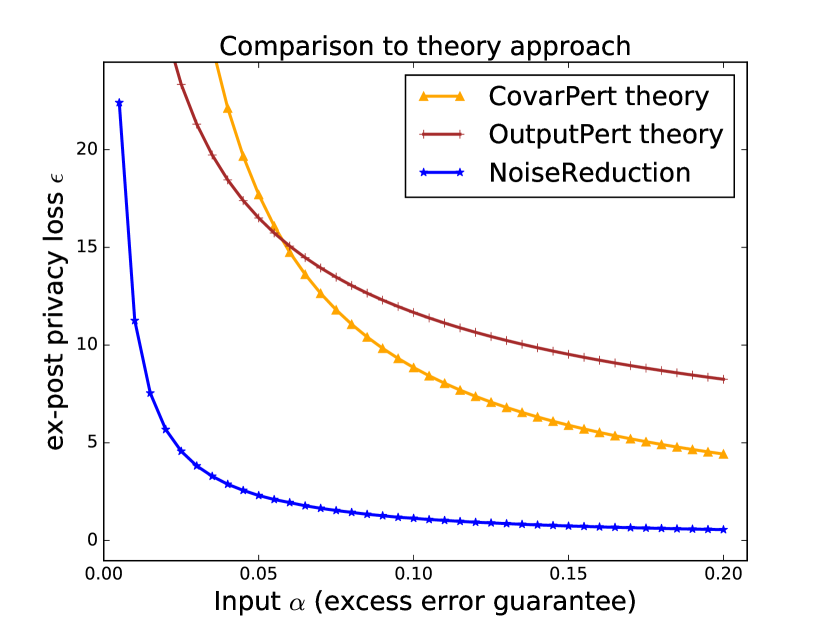
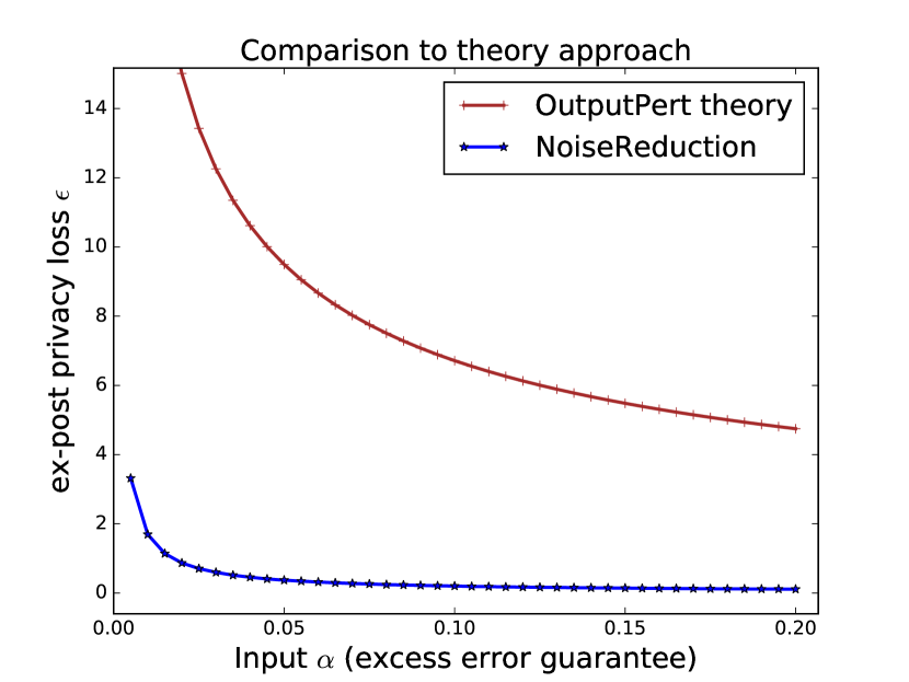
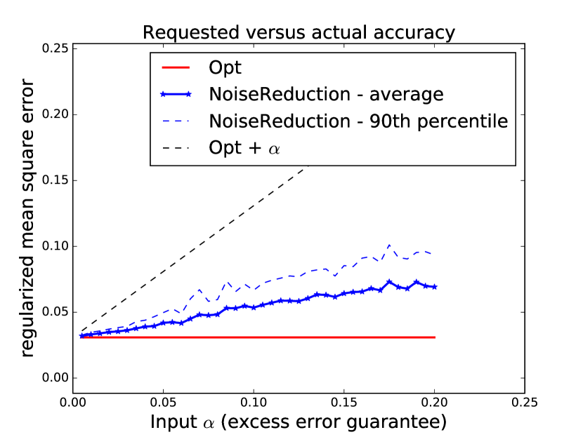
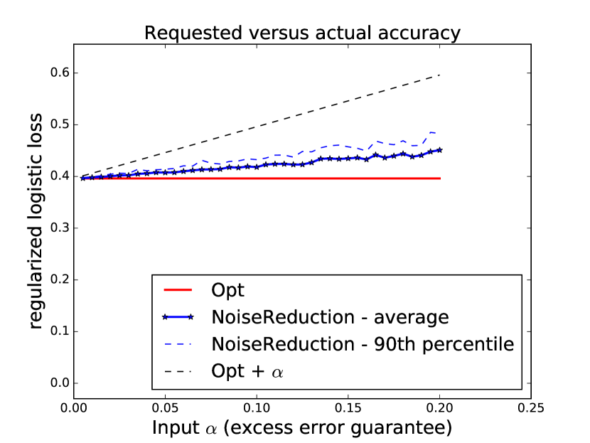
In each case, we tested the algorithm’s average ex-post privacy loss for a range of input accuracy goals α𝛼\alpha, fixing a modest failure probability γ=0.1𝛾0.1\gamma=0.1 (and we observed that excess risks were concentrated well below α/2𝛼2\alpha/2, suggesting a pessimistic analysis). The results show our meta-method gives a large improvement over the “theory” approach of simply inverting utility theorems for private ERM algorithms. (In fact, the utility theorem for the popular private stochastic gradient descent algorithm does not even give meaningful guarantees for the ranges of parameters tested; one would need an order of magnitude more data points, and even then the privacy losses are enormous, perhaps due to loose constants in the analysis.)

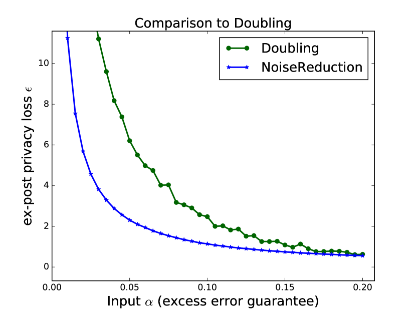
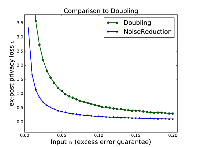
To gauge the more modest improvement over DoublingMethod, note that the variation in the privacy risk factor eεsuperscript𝑒𝜀e^{\varepsilon} can still be very large; for instance, in the ridge regression setting of α=0.05𝛼0.05\alpha=0.05, Noise Reduction has eε10.0superscript𝑒𝜀10.0e^{\varepsilon}\approx 10.0 while DoublingMethod has eε495superscript𝑒𝜀495e^{\varepsilon}\approx 495; at α=0.075𝛼0.075\alpha=0.075, the privacy risk factors are 4.654.654.65 and 56.656.656.6 respectively.

Refer to caption
(a) Linear (ridge) regression,
vs theory approach.
Refer to caption
(b) Regularized logistic regression,
vs theory approach.
Refer to caption
(c) Linear (ridge) regression,
vs DoublingMethod.
Refer to caption
(d) Regularized logistic regression,
vs DoublingMethod.
Figure 1: Ex-post privacy loss. (1(a)) and (1(c)), left, represent ridge regression on the Twitter dataset, where Noise Reduction and DoublingMethod both use Covariance Perturbation. (1(b)) and (1(d)), right, represent logistic regression on the KDD-99 Cup dataset, where both Noise Reduction and DoublingMethod use Output Perturbation. The top plots compare Noise Reduction to the “theory approach”: running the algorithm once using the value of ε𝜀\varepsilon that guarantees the desired expected error via a utility theorem. The bottom compares to the DoublingMethod baseline. Note the top plots are generous to the theory approach: the theory curves promise only expected error, whereas Noise Reduction promises a high probability guarantee. Each point is an average of 80 trials (Twitter dataset) or 40 trials (KDD-99 dataset).

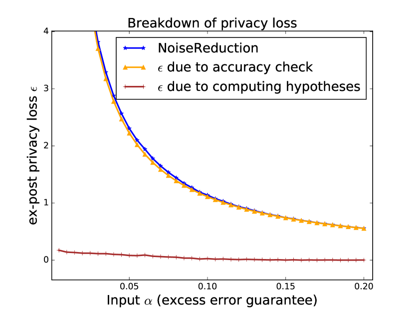
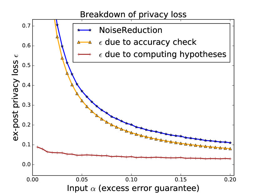
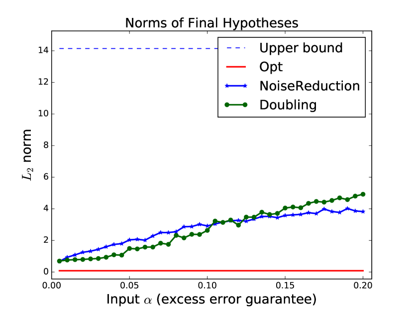
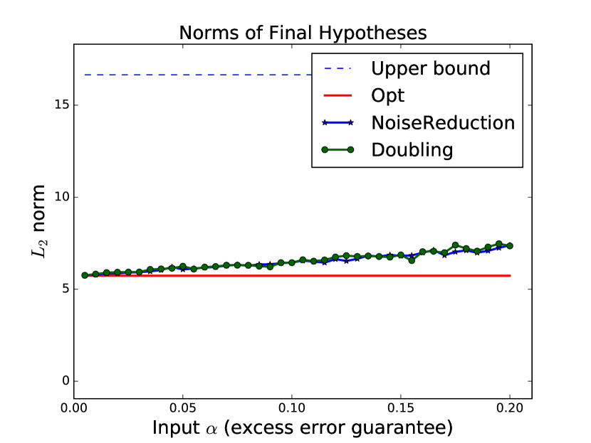
Interestingly, for our meta-method, the contribution to privacy loss from “testing” hypotheses (the InteractiveAboveThreshold technique) was significantly larger than that from “generating” them (NoiseReduction). One place where the InteractiveAboveThreshold analysis is loose is in using a theoretical bound on the maximum norm of any hypothesis to compute the sensitivity of queries. The actual norms of hypotheses tested was significantly lower which, if taken as guidance to the practitioner in advance, would drastically improve the privacy guarantee of both adaptive methods.

Acknowledgements

This work was supported in part by NSF grants CNS-1253345, CNS-1513694, CNS-1254169 and CNS-1518941, US-Israel Binational Science Foundation grant 2012348, Israeli Science Foundation (ISF) grant #1044/16, a subcontract on the DARPA Brandeis Project, the Warren Center for Data and Network Sciences, and the HUJI Cyber Security Research Center in conjunction with the Israel National Cyber Bureau in the Prime Minister’s Office.

References

  • [1] The AMA Team at Laboratoire d’Informatique de Grenoble. Buzz prediction in online social media, 2017.
  • [2] Raef Bassily, Adam D. Smith, and Abhradeep Thakurta. Private empirical risk minimization, revisited. CoRR, abs/1405.7085, 2014.
  • [3] Kamalika Chaudhuri and Claire Monteleoni. Privacy-preserving logistic regression. In Advances in Neural Information Processing Systems 21, Proceedings of the Twenty-Second Annual Conference on Neural Information Processing Systems, Vancouver, British Columbia, Canada, December 8-11, 2008, pages 289–296, 2008.
  • [4] Kamalika Chaudhuri, Claire Monteleoni, and Anand D. Sarwate. Differentially private empirical risk minimization. Journal of Machine Learning Research, 12:1069–1109, 2011.
  • [5] John C. Duchi, Michael I. Jordan, and Martin J. Wainwright. Local privacy and statistical minimax rates. In 51st Annual Allerton Conference on Communication, Control, and Computing, Allerton 2013, Allerton Park & Retreat Center, Monticello, IL, USA, October 2-4, 2013, page 1592, 2013.
  • [6] Cynthia Dwork, Frank McSherry, Kobbi Nissim, and Adam Smith. Calibrating noise to sensitivity in private data analysis. In Theory of Cryptography Conference, pages 265–284. Springer, 2006.
  • [7] Cynthia Dwork and Aaron Roth. The algorithmic foundations of differential privacy. Foundations and Trends® in Theoretical Computer Science, 9(3–4):211–407, 2014.
  • [8] Cynthia Dwork, Guy N Rothblum, and Salil Vadhan. Boosting and differential privacy. In Foundations of Computer Science (FOCS), 2010 51st Annual IEEE Symposium on, pages 51–60. IEEE, 2010.
  • [9] Giulia Fanti, Vasyl Pihur, and Úlfar Erlingsson. Building a rappor with the unknown: Privacy-preserving learning of associations and data dictionaries. Proceedings on Privacy Enhancing Technologies (PoPETS), issue 3, 2016, 2016.
  • [10] Andy Greenberg. Apple’s ’differential privacy’ is about collecting your data—but not your data. Wired Magazine, 2016.
  • [11] Prateek Jain, Pravesh Kothari, and Abhradeep Thakurta. Differentially private online learning. In COLT 2012 - The 25th Annual Conference on Learning Theory, June 25-27, 2012, Edinburgh, Scotland, pages 24.1–24.34, 2012.
  • [12] KDD’99. Kdd cup 1999 data, 1999.
  • [13] Daniel Kifer, Adam D. Smith, and Abhradeep Thakurta. Private convex optimization for empirical risk minimization with applications to high-dimensional regression. In COLT 2012 - The 25th Annual Conference on Learning Theory, June 25-27, 2012, Edinburgh, Scotland, pages 25.1–25.40, 2012.
  • [14] Fragkiskos Koufogiannis, Shuo Han, and George J. Pappas. Gradual release of sensitive data under differential privacy. Journal of Privacy and Confidentiality, 7, 2017.
  • [15] Frank McSherry and Kunal Talwar. Mechanism design via differential privacy. In Foundations of Computer Science, 2007. FOCS’07. 48th Annual IEEE Symposium on, pages 94–103. IEEE, 2007.
  • [16] Ryan M Rogers, Aaron Roth, Jonathan Ullman, and Salil Vadhan. Privacy odometers and filters: Pay-as-you-go composition. In D. D. Lee, M. Sugiyama, U. V. Luxburg, I. Guyon, and R. Garnett, editors, Advances in Neural Information Processing Systems 29, pages 1921–1929. Curran Associates, Inc., 2016.
  • [17] Benjamin I. P. Rubinstein, Peter L. Bartlett, Ling Huang, and Nina Taft. Learning in a large function space: Privacy-preserving mechanisms for SVM learning. CoRR, abs/0911.5708, 2009.
  • [18] Adam Smith, Jalaj Upadhyay, and Abhradeep Thakurta. Is interaction necessary for distributed private learning? IEEE Symposium on Security and Privacy, 2017.
  • [19] Shuang Song, Kamalika Chaudhuri, and Anand D. Sarwate. Stochastic gradient descent with differentially private updates. In IEEE Global Conference on Signal and Information Processing, GlobalSIP 2013, Austin, TX, USA, December 3-5, 2013, pages 245–248, 2013.
  • [20] Oliver Williams and Frank McSherry. Probabilistic inference and differential privacy. In Advances in Neural Information Processing Systems 23: 24th Annual Conference on Neural Information Processing Systems 2010. Proceedings of a meeting held 6-9 December 2010, Vancouver, British Columbia, Canada., pages 2451–2459, 2010.

Appendix A Missing Details and Proofs

A.1 AboveThreshold

Proof of Lemma 2.8.

Let D,D𝐷superscript𝐷D,D^{\prime} be neighboring databases. We will instead analyze the algorithm that outputs the entire prefix f1,,ftsubscript𝑓1subscript𝑓𝑡f_{1},\dots,f_{t} when stopping at time t𝑡t. Because IAT is a post-processing of this algorithm, and privacy can only be improved under post-processing, this suffices to prove the theorem. We wish to show for all outcomes o=(t,f1,,ft)𝑜𝑡subscript𝑓1subscript𝑓𝑡o=(t,f_{1},\dots,f_{t}):

Pr[IAT(D)=(t,f1,f2,,ft)]eεA+εtPr[IAT(D)=(t,f1,f2,,ft)].PrIAT𝐷𝑡subscript𝑓1subscript𝑓2subscript𝑓𝑡superscript𝑒subscript𝜀𝐴subscript𝜀𝑡PrIATsuperscript𝐷𝑡subscript𝑓1subscript𝑓2subscript𝑓𝑡\Pr\left[\textsc{IAT}(D)=(t,f_{1},f_{2},\ldots,f_{t})\right]\leq e^{\varepsilon_{A}+\varepsilon_{t}}\Pr\left[\textsc{IAT}(D^{\prime})=(t,f_{1},f_{2},\ldots,f_{t})\right].

We have directly from the privacy guarantee of InteractiveAboveThreshold that for every fixed sequence of queries f1,,ftsubscript𝑓1subscript𝑓𝑡f_{1},\ldots,f_{t}:

Pr[IAT(D)=tf1,,ft]eεAPr[IAT(D)=tf1,,ft]PrIAT𝐷conditional𝑡subscript𝑓1subscript𝑓𝑡superscript𝑒subscript𝜀𝐴PrIATsuperscript𝐷conditional𝑡subscript𝑓1subscript𝑓𝑡\Pr\left[\textsc{IAT}(D)=t\mid f_{1},\ldots,f_{t}\right]\leq e^{\varepsilon_{A}}\Pr\left[\textsc{IAT}(D^{\prime})=t\mid f_{1},\ldots,f_{t}\right] (2)

because the guarantee of InteractiveAboveThreshold is quantified over all data-independent sequences of queries f1,,fTsubscript𝑓1subscript𝑓𝑇f_{1},\ldots,f_{T}, and by definition of the algorithm, the probability of stopping at time t𝑡t is independent of the identity of any query ftsuperscriptsubscript𝑓𝑡f_{t}^{\prime} for t>tsuperscript𝑡𝑡t^{\prime}>t.

Now we can write:

Pr[IAT(D)=t,f1,ft]=Pr[IAT(D)=tf1,ft]Pr[M(D)=f1,ft].PrIAT𝐷𝑡subscript𝑓1subscript𝑓𝑡PrIAT𝐷conditional𝑡subscript𝑓1subscript𝑓𝑡Pr𝑀𝐷subscript𝑓1subscript𝑓𝑡\Pr\left[\textsc{IAT}(D)=t,f_{1},\ldots f_{t}\right]=\Pr\left[\textsc{IAT}(D)=t\mid f_{1},\ldots f_{t}\right]\Pr\left[M(D)=f_{1},\ldots f_{t}\right].

By assumption, M𝑀M is prefix-private, in particular, for fixed t𝑡t and any f1,,ftsubscript𝑓1subscript𝑓𝑡f_{1},\ldots,f_{t}:

Pr[M(D)=f1,ft]eεtPr[M(D)=f1,ft]Pr𝑀𝐷subscript𝑓1subscript𝑓𝑡superscript𝑒subscript𝜀𝑡Pr𝑀superscript𝐷subscript𝑓1subscript𝑓𝑡\Pr\left[M(D)=f_{1},\ldots f_{t}\right]\leq e^{\varepsilon_{t}}\Pr\left[M(D^{\prime})=f_{1},\ldots f_{t}\right]

Thus,

Pr[IAT(D)=t,f1,ft]Pr[IAT(D)=t,f1,ft]PrIAT𝐷𝑡subscript𝑓1subscript𝑓𝑡PrIATsuperscript𝐷𝑡subscript𝑓1subscript𝑓𝑡\displaystyle\frac{\Pr\left[\textsc{IAT}(D)=t,f_{1},\ldots f_{t}\right]}{\Pr\left[\textsc{IAT}(D^{\prime})=t,f_{1},\ldots f_{t}\right]} =Pr[IAT(D)=tf1,ft]Pr[IAT(D)=t|f1,,ft]Pr[M(D)=f1,ft]Pr[M(D)=f1,ft]absentPrIAT𝐷conditional𝑡subscript𝑓1subscript𝑓𝑡PrIATsuperscript𝐷conditional𝑡subscript𝑓1subscript𝑓𝑡Pr𝑀𝐷subscript𝑓1subscript𝑓𝑡Pr𝑀superscript𝐷subscript𝑓1subscript𝑓𝑡\displaystyle=\frac{\Pr\left[\textsc{IAT}(D)=t\mid f_{1},\ldots f_{t}\right]}{\Pr\left[\textsc{IAT}(D^{\prime})=t|f_{1},\ldots,f_{t}\right]}\frac{\Pr\left[M(D)=f_{1},\ldots f_{t}\right]}{\Pr\left[M(D^{\prime})=f_{1},\ldots f_{t}\right]}
eεAeεt=eεA+εt,absentsuperscript𝑒subscript𝜀𝐴superscript𝑒subscript𝜀𝑡superscript𝑒subscript𝜀𝐴subscript𝜀𝑡\displaystyle\leq e^{\varepsilon_{A}}\cdot e^{\varepsilon_{t}}=e^{\varepsilon_{A}+\varepsilon_{t}},

as desired. ∎

We also include the following utility theorem. We say that an instantiation of InteractiveAboveThreshold is (α,β)𝛼𝛽(\alpha,\beta) accurate with respect to a threshold W𝑊W and stream of queries f1,fTsubscript𝑓1subscript𝑓𝑇f_{1},\ldots f_{T} if except with probability at most γ𝛾\gamma, the algorithm outputs a query ftsubscript𝑓𝑡f_{t} only if ft(D)Wαsubscript𝑓𝑡𝐷𝑊𝛼f_{t}(D)\geq W-\alpha.

Theorem A.1.

For any sequence of 1-sensitive queries f1,,fTsubscript𝑓1subscript𝑓𝑇f_{1},\ldots,f_{T} such InteractiveAboveThreshold is (α,β)𝛼𝛽(\alpha,\beta)-accurate for

α=8Δ(log(T)+log(2/γ))ε.𝛼8Δ𝑇2𝛾𝜀\alpha=\frac{8\Delta(\log(T)+\log(2/\gamma))}{\varepsilon}.

A.2 Doubling Method

We now formally describe the DoublingMethod discussed in Section 1 and Section 3, and give a formal ex-post privacy analysis. Let θ=argminθpL(θ)superscript𝜃subscriptargmin𝜃superscript𝑝𝐿𝜃\theta^{*}=\operatorname*{\mathrm{argmin}}_{\theta\in\mathbb{R}^{p}}L(\theta). DoublingMethod accepts a list of privacy levels ε1<ε2<<εT,subscript𝜀1subscript𝜀2subscript𝜀𝑇\varepsilon_{1}<\varepsilon_{2}<\ldots<\varepsilon_{T}, where εi=2εi1subscript𝜀𝑖2subscript𝜀𝑖1\varepsilon_{i}=2\varepsilon_{i-1}. We show in B.1 that 222 is the optimal factor to scale ε𝜀\varepsilon by. It also takes in a failure probability γ𝛾\gamma, and a black-box private ERM mechanism M𝑀M that has the following guarantee: Fixing a dataset D𝐷D, M𝑀M takes as input D𝐷D and a privacy level εisubscript𝜀𝑖\varepsilon_{i}, and generates an εisubscript𝜀𝑖\varepsilon_{i}-differentially private hypothesis θisubscript𝜃𝑖\theta_{i}, such that the query fi(D)=L(D,θ)L(D,θi)f^{i}(D)=L(D,\theta*)-L(D,\theta_{i}) has 1subscript1\ell_{1} sensitivity at most ΔΔ\Delta.

Algorithm 4 Doubling Method: DoublingMethod(D,{ε1,,εT},M,α,γ)DoublingMethod𝐷subscript𝜀1subscript𝜀𝑇𝑀𝛼𝛾\textsc{DoublingMethod}(D,\{\varepsilon_{1},\ldots,\varepsilon_{T}\},M,\alpha,\gamma)
Input: private dataset D𝐷D, accuracy α𝛼\alpha, failure probability γ𝛾\gamma, mechanism M𝑀M
for each t=1,,T𝑡1𝑇t=1,\dots,T do
     Generate θtM(D)tsubscript𝜃𝑡𝑀subscript𝐷𝑡\theta_{t}\leftarrow M(D)_{t}
     Let ft(D)=L(D,θ)L(D,θt)superscript𝑓𝑡𝐷𝐿𝐷superscript𝜃𝐿𝐷subscript𝜃𝑡f^{t}(D)=L(D,\theta^{*})-L(D,\theta_{t})
     Generate wtLap(α2log(Tγ))similar-tosubscript𝑤𝑡Lap𝛼2𝑇𝛾w_{t}\sim\text{Lap}\left({\frac{\alpha}{2\log(\frac{T}{\gamma})}}\right)
     if ft(D)+wtα/2superscript𝑓𝑡𝐷subscript𝑤𝑡𝛼2f^{t}(D)+w_{t}\geq-\alpha/2then Output (t𝑡t, ftsuperscript𝑓𝑡f^{t}); Halt.      
Output T+1,θ𝑇1superscript𝜃T+1,\theta^{*}.
Theorem A.2.

For kT𝑘𝑇k\leq T, define the privacy loss function (k,θk)=2kΔlog(T/γ)α+(2k1)ε1,and(T+1,θ)=formulae-sequence𝑘subscript𝜃𝑘2𝑘Δ𝑇𝛾𝛼superscript2𝑘1subscript𝜀1𝑎𝑛𝑑𝑇1superscript𝜃\mathcal{E}(k,\theta_{k})=\frac{2k\Delta\log(T/\gamma)}{\alpha}+(2^{k}-1)\varepsilon_{1},and\mathcal{E}(T+1,\theta^{*})=\infty. Then DoublingMethod is \mathcal{E}-ex-post differentially private, and is 1γ1𝛾1-\gamma accurate.

Proof.

Since if the algorithm reaches step T+1𝑇1T+1 it outputs the true minimizer which has error 0<α0𝛼0<\alpha, it could only fail to output a hypothesis with error less than α𝛼\alpha if it stops at iT𝑖𝑇i\leq T. DoublingMethod only stops early if the noisy query is greater than α/2𝛼2-\alpha/2; or fi(D)+wiα/2superscript𝑓𝑖𝐷subscript𝑤𝑖𝛼2f^{i}(D)+w_{i}\geq-\alpha/2. But fi(D)αsuperscript𝑓𝑖𝐷𝛼f^{i}(D)\leq-\alpha, which forces wiα/2subscript𝑤𝑖𝛼2w_{i}\geq\alpha/2. By properties of the Laplace distribution, Pr[wiα/2]=12exp(α22log(T2γ)α)=γ/TPrsubscript𝑤𝑖𝛼212exp𝛼22𝑇2𝛾𝛼𝛾𝑇\Pr\left[w_{i}\geq\alpha/2\right]=\frac{1}{2}\text{exp}(\frac{-\alpha}{2}\frac{2\log(\frac{T}{2\gamma})}{\alpha})=\gamma/T. Hence by union bound over T𝑇T the total failure probability is at most γ𝛾\gamma.

By the assumption, generating the kthsuperscript𝑘𝑡k^{th} private hypothesis incurs privacy loss ε12k1subscript𝜀1superscript2𝑘1\varepsilon_{1}*2^{k-1}. By the Laplace mechanism, evaluating the error of the sensitivity ΔΔ\Delta query fisuperscript𝑓𝑖f^{i} is 2Δlog(T/γ)α2Δ𝑇𝛾𝛼\frac{2\Delta\log(T/\gamma)}{\alpha}-differentially private. Theorem 3.63.63.6 in [16] then says that the ex-post privacy loss of outputting kT𝑘𝑇k\leq T is i=1k[ε12k1+2Δlog(T/γ)α]=2kΔlog(T/γ)α+(2k1)ε1superscriptsubscript𝑖1𝑘delimited-[]subscript𝜀1superscript2𝑘12Δ𝑇𝛾𝛼2𝑘Δ𝑇𝛾𝛼superscript2𝑘1subscript𝜀1\sum_{i=1}^{k}[\varepsilon_{1}*2^{k-1}+\frac{2\Delta\log(T/\gamma)}{\alpha}]=\frac{2k\Delta\log(T/\gamma)}{\alpha}+(2^{k}-1)\varepsilon_{1}, as desired. ∎

Remark A.3.

In practice, the private empirical risk minimization mechanism M𝑀M may not always output a hypothesis that leads to queries with uniformly bounded 1subscript1\ell_{1} sensitivity. In this case, a projection that scales down, the hypothesis norm can be applied prior to evaluating the private query error. For a discussion of scaling the norm down refer to the experiments section of the appendix.

A.3 Ridge Regression

In this subsection, we let (θ,(Xi,yi))=12(yiθ,Xi)2𝜃subscript𝑋𝑖subscript𝑦𝑖12superscriptsubscript𝑦𝑖𝜃subscript𝑋𝑖2\ell(\theta,(X_{i},y_{i}))=\frac{1}{2}(y_{i}-\langle\theta,X_{i}\rangle)^{2}, and the empirical loss over the data set is defined as

L(D,θ)=12nyXθ22+λθ222,𝐿𝐷𝜃12𝑛subscriptsuperscriptnorm𝑦𝑋𝜃22𝜆superscriptsubscriptnorm𝜃222L(D,\theta)=\frac{1}{2n}\|y-X\theta\|^{2}_{2}+\frac{\lambda\|\theta\|_{2}^{2}}{2},

where X𝑋X denotes the (n×p)𝑛𝑝(n\times p) matrix with row vectors X1,,Xnsubscript𝑋1subscript𝑋𝑛X_{1},\ldots,X_{n} and y=(y1,,yn)𝑦subscript𝑦1subscript𝑦𝑛y=(y_{1},\ldots,y_{n}). We assume that for each i𝑖i, Xi11subscriptnormsubscript𝑋𝑖11\|X_{i}\|_{1}\leq 1 and |yi|1subscript𝑦𝑖1|y_{i}|\leq 1. For simplicity, we will sometimes write L(θ)𝐿𝜃L(\theta) for L(D,θ)𝐿𝐷𝜃L(D,\theta).

First, we show that the unconstrained optimal solution in ridge regression has bounded norm.

Lemma A.4.

Let θ=argminθdL(θ)superscript𝜃subscriptargmin𝜃superscript𝑑𝐿𝜃\theta^{*}=\operatorname*{\mathrm{argmin}}_{\theta\in\mathbb{R}^{d}}L(\theta). Then θ21λsubscriptnormsuperscript𝜃21𝜆||\theta^{*}||_{2}\leq\frac{1}{\sqrt{\lambda}}.

Proof.

For any θp,L(θ)L(θ)formulae-sequence𝜃superscript𝑝𝐿superscript𝜃𝐿𝜃\theta\in\mathbb{R}^{p},L(\theta^{*})\leq L(\theta). In particular for θ=𝟎𝜃0\theta=\mathbf{0},

L(θ)L(𝟎)=i=1n12n((Xi,yi),0)12.𝐿superscript𝜃𝐿0superscriptsubscript𝑖1𝑛12𝑛subscript𝑋𝑖subscript𝑦𝑖012L(\theta^{*})\leq L(\mathbf{0})=\sum_{i=1}^{n}\frac{1}{2n}\ell((X_{i},y_{i}),0)\leq\frac{1}{2}.

Note that for any θ,((Xi,yi),θ)0𝜃subscript𝑋𝑖subscript𝑦𝑖𝜃0\theta,\ell((X_{i},y_{i}),\theta)\geq 0, so this means L(θ)λ2θ22𝐿superscript𝜃𝜆2superscriptsubscriptnormsuperscript𝜃22L(\theta^{*})\geq\frac{\lambda}{2}||\theta^{*}||_{2}^{2}, which forces λ2θ2212𝜆2superscriptsubscriptnormsuperscript𝜃2212\frac{\lambda}{2}||\theta^{*}||_{2}^{2}\leq\frac{1}{2}, and so θ21λsubscriptnormsuperscript𝜃21𝜆||\theta^{*}||_{2}\leq\frac{1}{\sqrt{\lambda}} as desired. ∎

The following claim provides a bound on the sensitivity for the excess risk, which are the queries we send to InteractiveAboveThreshold.

Claim A.5.

Let C𝐶C be a bounded convex set in psuperscript𝑝\mathbb{R}^{p} with C2Msubscriptnorm𝐶2𝑀\|C\|_{2}\leq M. Let D𝐷D and Dsuperscript𝐷D^{\prime} be a pair of adjacent datasets, and let θ=argminθCL(θ,D)superscript𝜃subscriptargmin𝜃𝐶𝐿𝜃𝐷\theta^{*}=\operatorname*{\mathrm{argmin}}_{\theta\in C}L(\theta,D) and θ=argminθCL(θ,D)superscript𝜃subscriptargmin𝜃𝐶𝐿𝜃superscript𝐷\theta^{\bullet}=\operatorname*{\mathrm{argmin}}_{\theta\in C}L(\theta,D^{\prime}). Then for any θC𝜃𝐶\theta\in C,

|(L(θ,D)L(θ,D))(L(θ,D)L(θ,D))|(M+1)2n.𝐿𝜃𝐷𝐿superscript𝜃𝐷𝐿𝜃superscript𝐷𝐿superscript𝜃superscript𝐷superscript𝑀12𝑛|(L(\theta,D)-L(\theta^{*},D))-(L(\theta,D^{\prime})-L(\theta^{\bullet},D^{\prime}))|\leq\frac{(M+1)^{2}}{n}.

The following lemma provides a bound on the 1subscript1\ell_{1} sensitivity for the matrix XXsuperscript𝑋𝑋X^{\intercal}X and vector Xysuperscript𝑋𝑦X^{\intercal}y.

Lemma A.6.

Fix any i[n]𝑖delimited-[]𝑛i\in[n]. Let X𝑋X and Z𝑍Z be two n×p𝑛𝑝n\times p matrices such that for all rows ji𝑗𝑖j\neq i, Xj=Zjsubscript𝑋𝑗subscript𝑍𝑗X_{j}=Z_{j}. Let y,yn𝑦superscript𝑦superscript𝑛y,y^{\prime}\in\mathbb{R}^{n} such that yj=yjsubscript𝑦𝑗superscriptsubscript𝑦𝑗y_{j}=y_{j}^{\prime} for all ji𝑗𝑖j\neq i. Then

XXZZ12 and XyZy12,formulae-sequencesubscriptnormsuperscript𝑋𝑋superscript𝑍𝑍12 and subscriptnormsuperscript𝑋𝑦superscript𝑍superscript𝑦12\|X^{\intercal}X-Z^{\intercal}Z\|_{1}\leq 2\quad\mbox{ and }\quad\|X^{\intercal}y-Z^{\intercal}y^{\prime}\|_{1}\leq 2,

as long as Xi,Zi,|yi|,|yi|1normsubscript𝑋𝑖normsubscript𝑍𝑖subscript𝑦𝑖superscriptsubscript𝑦𝑖1\|X_{i}\|,\|Z_{i}\|,|y_{i}|,|y_{i}^{\prime}|\leq 1.

Proof.

We can write

XXZZ1subscriptnormsuperscript𝑋𝑋superscript𝑍𝑍1\displaystyle\|X^{\intercal}X-Z^{\intercal}Z\|_{1} =j(XjXjZjZj)1absentsubscriptnormsubscript𝑗subscriptsuperscript𝑋𝑗subscript𝑋𝑗subscriptsuperscript𝑍𝑗subscript𝑍𝑗1\displaystyle=\|\sum_{j}\left(X^{\intercal}_{j}X_{j}-Z^{\intercal}_{j}Z_{j}\right)\|_{1}
=XiXiZiZ1absentsubscriptnormsubscriptsuperscript𝑋𝑖subscript𝑋𝑖subscriptsuperscript𝑍𝑖𝑍1\displaystyle=\|X^{\intercal}_{i}X_{i}-Z^{\intercal}_{i}Z\|_{1}
XiXi1+ZiZi1absentsubscriptnormsubscriptsuperscript𝑋𝑖subscript𝑋𝑖1subscriptnormsubscriptsuperscript𝑍𝑖subscript𝑍𝑖1\displaystyle\leq\|X^{\intercal}_{i}X_{i}\|_{1}+\|Z^{\intercal}_{i}Z_{i}\|_{1}
=Xi12+Zi122.absentsuperscriptsubscriptnormsubscript𝑋𝑖12superscriptsubscriptnormsubscript𝑍𝑖122\displaystyle=\|X_{i}\|_{1}^{2}+\|Z_{i}\|_{1}^{2}\leq 2.

Similarly,

XyZy1subscriptnormsuperscript𝑋𝑦superscript𝑍superscript𝑦1\displaystyle\|X^{\intercal}y-Z^{\intercal}y^{\prime}\|_{1} =j(yjXjyjZj)1absentsubscriptnormsubscript𝑗subscript𝑦𝑗subscript𝑋𝑗subscriptsuperscript𝑦𝑗subscript𝑍𝑗1\displaystyle=\|\sum_{j}\left(y_{j}X_{j}-y^{\prime}_{j}Z_{j}\right)\|_{1}
=yiXiyiZi1absentsubscriptnormsubscript𝑦𝑖subscript𝑋𝑖subscriptsuperscript𝑦𝑖subscript𝑍𝑖1\displaystyle=\|y_{i}X_{i}-y^{\prime}_{i}Z_{i}\|_{1}
=yiXi1+yiZi1absentsubscriptnormsubscript𝑦𝑖subscript𝑋𝑖1subscriptnormsubscriptsuperscript𝑦𝑖subscript𝑍𝑖1\displaystyle=\|y_{i}X_{i}\|_{1}+\|y^{\prime}_{i}Z_{i}\|_{1}
=Xi1+Zi12.absentsubscriptnormsubscript𝑋𝑖1subscriptnormsubscript𝑍𝑖12\displaystyle=\|X_{i}\|_{1}+\|Z_{i}\|_{1}\leq 2.

This completes the proof. ∎

Before we proceed to give a formal proof for Theorem 3.1, we will also give the following basic fact about Laplace random vectors.

Claim A.7.

Let ν=(ν1,,νk)k𝜈subscript𝜈1subscript𝜈𝑘superscript𝑘\nu=(\nu_{1},\ldots,\nu_{k})\in\mathbb{R}^{k} such that each νisubscript𝜈𝑖\nu_{i} is an independent random variable drawn from the Laplace distribution Lap(r)Lap𝑟\text{Lap}\left({r}\right). Then 𝔼[ν2]2kr𝔼subscriptnorm𝜈22𝑘𝑟\operatorname*{\mathbb{E}}\left[\|\nu\|_{2}\right]\leq\sqrt{2k}r.

Proof.

By Jensen’s inequality,

𝔼[ν2]=𝔼[iνi2]𝔼[iνi2].𝔼subscriptnorm𝜈2𝔼subscript𝑖superscriptsubscript𝜈𝑖2𝔼subscript𝑖superscriptsubscript𝜈𝑖2\operatorname*{\mathbb{E}}\left[\|\nu\|_{2}\right]=\operatorname*{\mathbb{E}}\left[\sqrt{\sum_{i}\nu_{i}^{2}}\right]\leq\sqrt{\operatorname*{\mathbb{E}}\left[\sum_{i}\nu_{i}^{2}\right]}.

Note that by linearity of expectation and the variance of the Laplace distribution

𝔼[iνi2]=i𝔼[νi2]=i2r2=2kr2.𝔼subscript𝑖superscriptsubscript𝜈𝑖2subscript𝑖𝔼superscriptsubscript𝜈𝑖2subscript𝑖2superscript𝑟22𝑘superscript𝑟2\operatorname*{\mathbb{E}}\left[\sum_{i}\nu_{i}^{2}\right]=\sum_{i}\operatorname*{\mathbb{E}}\left[\nu_{i}^{2}\right]=\sum_{i}2r^{2}=2kr^{2}.

Therefore, we have 𝔼[ν2]2kr𝔼subscriptnorm𝜈22𝑘𝑟\operatorname*{\mathbb{E}}\left[\|\nu\|_{2}\right]\leq\sqrt{2k}r. ∎

Proof of Theorem 3.1.

In the algorithm, we compute Z=XX+B𝑍superscript𝑋𝑋𝐵Z=X^{\intercal}X+B and z=Xy+b𝑧superscript𝑋𝑦𝑏z=X^{\intercal}y+b, where the entries of B𝐵B and b𝑏b are drawn i.i.d. from Lap(4/ε)Lap4𝜀\text{Lap}\left({4/\varepsilon}\right). Note that the output θpsubscript𝜃𝑝\theta_{p} is simply a post-processing of the noisy matrix Z𝑍Z and vector z𝑧z. Furthermore, by Lemma A.6, the joint vector (Z,z)𝑍𝑧(Z,z) is has sensitivity bounded by 4 with respect to 1subscript1\ell_{1} norm. Therefore, the mechanism satisfies ε𝜀\varepsilon-differential privacy by the privacy guarantee of the Laplace mechanism.

Let M=1/λ𝑀1𝜆M=\sqrt{1/\lambda} and Lp(θ)=12n(2z,θ)+12n(θZθ)+λθ222subscript𝐿𝑝𝜃12𝑛2𝑧𝜃12𝑛superscript𝜃𝑍𝜃𝜆superscriptsubscriptnorm𝜃222L_{p}(\theta)=\frac{1}{2n}\left(-2\langle z,\theta\rangle\right)+\frac{1}{2n}(\theta^{\intercal}Z\theta)+\frac{\lambda\|\theta\|_{2}^{2}}{2}. Observe that θp=argminθCLp(θ)subscript𝜃𝑝subscriptargmin𝜃𝐶subscript𝐿𝑝𝜃\theta_{p}=\operatorname*{\mathrm{argmin}}_{\theta\in C}L_{p}(\theta). Our goal is to bound L(θp)L(θ)𝐿subscript𝜃𝑝𝐿superscript𝜃L(\theta_{p})-L(\theta^{*}), which can be written as follows

L(θp)L(θ)𝐿subscript𝜃𝑝𝐿superscript𝜃\displaystyle L(\theta_{p})-L(\theta^{*}) =L(θp)Lp(θp)+Lp(θp)Lp(θ)+Lp(θ)L(θ)absent𝐿subscript𝜃𝑝subscript𝐿𝑝subscript𝜃𝑝subscript𝐿𝑝subscript𝜃𝑝subscript𝐿𝑝superscript𝜃subscript𝐿𝑝superscript𝜃𝐿superscript𝜃\displaystyle=L(\theta_{p})-L_{p}(\theta_{p})+L_{p}(\theta_{p})-L_{p}(\theta^{*})+L_{p}(\theta^{*})-L(\theta^{*})
L(θp)Lp(θp)+Lp(θ)L(θ)absent𝐿subscript𝜃𝑝subscript𝐿𝑝subscript𝜃𝑝subscript𝐿𝑝superscript𝜃𝐿superscript𝜃\displaystyle\leq L(\theta_{p})-L_{p}(\theta_{p})+L_{p}(\theta^{*})-L(\theta^{*})
=12n(2b,θpθpBθp)12n(2b,θ(θ)Bθ)absent12𝑛2𝑏subscript𝜃𝑝superscriptsubscript𝜃𝑝𝐵subscript𝜃𝑝12𝑛2𝑏superscript𝜃superscriptsuperscript𝜃𝐵superscript𝜃\displaystyle=\frac{1}{2n}\left(2\langle b,\theta_{p}\rangle-\theta_{p}^{\intercal}B\theta_{p}\right)-\frac{1}{2n}\left(2\langle b,\theta^{*}\rangle-(\theta^{*})^{\intercal}B\theta^{*}\right)

Moreover, b,θpb2θp2Mb2𝑏subscript𝜃𝑝subscriptnorm𝑏2subscriptnormsubscript𝜃𝑝2𝑀subscriptnorm𝑏2\langle b,\theta_{p}\rangle\leq\|b\|_{2}\|\theta_{p}\|_{2}\leq M\|b\|_{2} and

θpBθpsuperscriptsubscript𝜃𝑝𝐵subscript𝜃𝑝\displaystyle-\theta_{p}^{\intercal}B\theta_{p} =(s,t)[p]2Bst(θp)s(θp)tabsentsubscript𝑠𝑡superscriptdelimited-[]𝑝2subscript𝐵𝑠𝑡subscriptsubscript𝜃𝑝𝑠subscriptsubscript𝜃𝑝𝑡\displaystyle=-\sum_{(s,t)\in[p]^{2}}B_{st}(\theta_{p})_{s}(\theta_{p})_{t}
((s,t)Bst2)1/2(s,t(θp)s2(θp)t2)1/2absentsuperscriptsubscript𝑠𝑡superscriptsubscript𝐵𝑠𝑡212superscriptsubscript𝑠𝑡superscriptsubscriptsubscript𝜃𝑝𝑠2superscriptsubscriptsubscript𝜃𝑝𝑡212\displaystyle\leq\left(\sum_{(s,t)}B_{st}^{2}\right)^{1/2}\left(\sum_{s,t}(\theta_{p})_{s}^{2}(\theta_{p})_{t}^{2}\right)^{1/2}
=BF[(s(θp)s2)2]1/2absentsubscriptnorm𝐵𝐹superscriptdelimited-[]superscriptsubscript𝑠superscriptsubscriptsubscript𝜃𝑝𝑠2212\displaystyle=\|B\|_{F}\left[\left(\sum_{s}(\theta_{p})_{s}^{2}\right)^{2}\right]^{1/2}
BFM2absentsubscriptnorm𝐵𝐹superscript𝑀2\displaystyle\leq\|B\|_{F}M^{2}

By A.7, we also have 𝔼[BF]42p/ε𝔼subscriptnorm𝐵𝐹42𝑝𝜀\operatorname*{\mathbb{E}}\left[\|B\|_{F}\right]\leq 4\sqrt{2}p/\varepsilon and 𝔼[b2]42p/ε𝔼subscriptnorm𝑏242𝑝𝜀\operatorname*{\mathbb{E}}\left[\|b\|_{2}\right]\leq 4\sqrt{2p}/\varepsilon. Finally,

𝔼[L(θp)L(θ)]𝔼𝐿subscript𝜃𝑝𝐿superscript𝜃\displaystyle\operatorname*{\mathbb{E}}\left[L(\theta_{p})-L(\theta^{*})\right] 𝔼[12n(2b,θpθpBθp)12n(2b,θ(θ)Bθ)]absent𝔼12𝑛2𝑏subscript𝜃𝑝superscriptsubscript𝜃𝑝𝐵subscript𝜃𝑝12𝑛2𝑏superscript𝜃superscriptsuperscript𝜃𝐵superscript𝜃\displaystyle\leq\operatorname*{\mathbb{E}}\left[\frac{1}{2n}\left(2\langle b,\theta_{p}\rangle-\theta_{p}^{\intercal}B\theta_{p}\right)-\frac{1}{2n}\left(2\langle b,\theta^{*}\rangle-(\theta^{*})^{\intercal}B\theta^{*}\right)\right]
=𝔼[2b,θpθpBθp2n]absent𝔼2𝑏subscript𝜃𝑝superscriptsubscript𝜃𝑝𝐵subscript𝜃𝑝2𝑛\displaystyle=\operatorname*{\mathbb{E}}\left[\frac{2\langle b,\theta_{p}\rangle-\theta_{p}^{\intercal}B\theta_{p}}{2n}\right]
𝔼[2Mb2]+𝔼[M2BF]2nabsent𝔼2𝑀subscriptnorm𝑏2𝔼superscript𝑀2subscriptnorm𝐵𝐹2𝑛\displaystyle\leq\frac{\operatorname*{\mathbb{E}}\left[2M\|b\|_{2}\right]+\operatorname*{\mathbb{E}}\left[M^{2}\|B\|_{F}\right]}{2n}
42(2pM+pM2)nεabsent422𝑝𝑀𝑝superscript𝑀2𝑛𝜀\displaystyle\leq\frac{4\sqrt{2}(2\sqrt{p}M+pM^{2})}{n\varepsilon}

which recovers our stated bound. ∎

Next, we will also provide a theoretical result for applying output perturbation (with Laplace noise) to the ridge regression problem. This will provides us the “theory curve” for output perturbation in ridge regression plot of Figure 1(a).

First, the following sensitivity bound on the optimal solution for L𝐿L follows directly from the strong convexity of L𝐿L.

Lemma A.8.

Let C𝐶C be a bounded convex set in psuperscript𝑝\mathbb{R}^{p} with C2Msubscriptnorm𝐶2𝑀\|C\|_{2}\leq M. Let D𝐷D and Dsuperscript𝐷D^{\prime} be a pair of neighboring datasets, and let θ=argminθCL(θ,D)superscript𝜃subscriptargmin𝜃𝐶𝐿𝜃𝐷\theta^{*}=\operatorname*{\mathrm{argmin}}_{\theta\in C}L(\theta,D) and θ=argminθCL(θ,D)superscript𝜃subscriptargmin𝜃𝐶𝐿𝜃superscript𝐷\theta^{\bullet}=\operatorname*{\mathrm{argmin}}_{\theta\in C}L(\theta,D^{\prime}). Then θθ1(M+1)pnλsubscriptnormsuperscript𝜃superscript𝜃1𝑀1𝑝𝑛𝜆\|\theta^{*}-\theta^{\bullet}\|_{1}\leq(M+1)\sqrt{\frac{p}{n\lambda}}.

Theorem A.9.

Let ε>0𝜀0\varepsilon>0 and C𝐶C be a bounded convex set with C21/λsubscriptnorm𝐶21𝜆\|C\|_{2}\leq\sqrt{1/\lambda}. Let r=(1/λ+1)p/(nλ)/ε𝑟1𝜆1𝑝𝑛𝜆𝜀r=(\sqrt{1/\lambda}+1)\sqrt{p/(n\lambda)}/\varepsilon. Consider the following mechanism \mathcal{M} that for any input dataset D𝐷D first computes the optimal solution θ=argminθCL(θ)superscript𝜃subscriptargmin𝜃𝐶𝐿𝜃\theta^{*}=\operatorname*{\mathrm{argmin}}_{\theta\in C}L(\theta), and then outputs θp=θ+bsubscript𝜃𝑝superscript𝜃𝑏\theta_{p}=\theta^{*}+b, where b𝑏b is a random vector with its entries drawn i.i.d. from Lap(r)Lap𝑟\text{Lap}\left({r}\right). Then \mathcal{M} satisfies ε𝜀\varepsilon-differential privacy, and θpsubscript𝜃𝑝\theta_{p} satisfies

𝔼b[L(θp)L(θ)]=(1n+λ)(1/λ+1)2p2nλε2.\operatorname*{\mathbb{E}}_{b}\left[L(\theta_{p})-L(\theta^{*})\right]\leq=\left(\frac{1}{n}+\lambda\right)\frac{(\sqrt{1/\lambda}+1)^{2}p^{2}}{n\lambda\varepsilon^{2}}.
Proof.

The privacy guarantee follows directly from the use of Laplace mechanism and the 1subscript1\ell_{1} sensitivity bound in Lemma A.8.

For each data point di=(Xi,yi)subscript𝑑𝑖subscript𝑋𝑖subscript𝑦𝑖d_{i}=(X_{i},y_{i}), we have

(yiθp,Xi)2(yiθ,Xi)2superscriptsubscript𝑦𝑖subscript𝜃𝑝subscript𝑋𝑖2superscriptsubscript𝑦𝑖superscript𝜃subscript𝑋𝑖2\displaystyle(y_{i}-\langle\theta_{p},X_{i}\rangle)^{2}-(y_{i}-\langle\theta^{*},X_{i}\rangle)^{2} =(θp,Xi)2(θ,Xi)22b,Xiabsentsuperscriptsubscript𝜃𝑝subscript𝑋𝑖2superscriptsuperscript𝜃subscript𝑋𝑖22𝑏subscript𝑋𝑖\displaystyle=(\langle\theta_{p},X_{i}\rangle)^{2}-(\langle\theta^{*},X_{i}\rangle)^{2}-2\langle b,X_{i}\rangle
=b(XiXi)b+(θ)(XiXi)b+b(XiXi)θ2b,Xiabsentsuperscript𝑏superscriptsubscript𝑋𝑖subscript𝑋𝑖𝑏superscriptsuperscript𝜃superscriptsubscript𝑋𝑖subscript𝑋𝑖𝑏superscript𝑏superscriptsubscript𝑋𝑖subscript𝑋𝑖superscript𝜃2𝑏subscript𝑋𝑖\displaystyle=b^{\intercal}(X_{i}^{\intercal}X_{i})b+(\theta^{*})^{\intercal}(X_{i}^{\intercal}X_{i})b+b^{\intercal}(X_{i}^{\intercal}X_{i})\theta^{*}-2\langle b,X_{i}\rangle

Since each entry in b𝑏b has mean 0, we can simplify the expectation as

𝔼[(yiθp,Xi)2(yiθ,Xi)2]𝔼superscriptsubscript𝑦𝑖subscript𝜃𝑝subscript𝑋𝑖2superscriptsubscript𝑦𝑖superscript𝜃subscript𝑋𝑖2\displaystyle\operatorname*{\mathbb{E}}\left[(y_{i}-\langle\theta_{p},X_{i}\rangle)^{2}-(y_{i}-\langle\theta^{*},X_{i}\rangle)^{2}\right] =𝔼[b(XiXi)b]absent𝔼superscript𝑏superscriptsubscript𝑋𝑖subscript𝑋𝑖𝑏\displaystyle=\operatorname*{\mathbb{E}}\left[b^{\intercal}(X_{i}^{\intercal}X_{i})b\right]
=𝔼[(b,Xi)2]absent𝔼superscript𝑏subscript𝑋𝑖2\displaystyle=\operatorname*{\mathbb{E}}\left[\left(\langle b,X_{i}\rangle\right)^{2}\right]
𝔼[b22Xi22]absent𝔼superscriptsubscriptnorm𝑏22superscriptsubscriptnormsubscript𝑋𝑖22\displaystyle\leq\operatorname*{\mathbb{E}}\left[\|b\|_{2}^{2}\|X_{i}\|_{2}^{2}\right]
=𝔼[b22]𝔼[Xi22]absent𝔼superscriptsubscriptnorm𝑏22𝔼superscriptsubscriptnormsubscript𝑋𝑖22\displaystyle=\operatorname*{\mathbb{E}}\left[\|b\|_{2}^{2}\right]\operatorname*{\mathbb{E}}\left[\|X_{i}\|_{2}^{2}\right]
𝔼[b22]2pr2absent𝔼superscriptsubscriptnorm𝑏222𝑝superscript𝑟2\displaystyle\leq\operatorname*{\mathbb{E}}\left[\|b\|_{2}^{2}\right]\leq 2pr^{2}

In the following, let M=1/λ𝑀1𝜆M=\sqrt{1/\lambda}. We can then bound

θp22θ22superscriptsubscriptnormsubscript𝜃𝑝22superscriptsubscriptnormsuperscript𝜃22\displaystyle\|\theta_{p}\|_{2}^{2}-\|\theta^{*}\|_{2}^{2} =s[p][(θs+bs)2θs2]absentsubscript𝑠delimited-[]𝑝delimited-[]superscriptsubscript𝜃𝑠subscript𝑏𝑠2superscriptsubscript𝜃𝑠2\displaystyle=\sum_{s\in[p]}\left[(\theta_{s}+b_{s})^{2}-\theta_{s}^{2}\right]
=s[p][2θsbs+bs2],absentsubscript𝑠delimited-[]𝑝delimited-[]2subscript𝜃𝑠subscript𝑏𝑠superscriptsubscript𝑏𝑠2\displaystyle=\sum_{s\in[p]}\left[2\theta_{s}b_{s}+b_{s}^{2}\right],

Again, since each bssubscript𝑏𝑠b_{s} is drawn from Lap(r)Lap𝑟\text{Lap}\left({r}\right), we get

𝔼[θp22θ22]𝔼superscriptsubscriptnormsubscript𝜃𝑝22superscriptsubscriptnormsuperscript𝜃22\displaystyle\operatorname*{\mathbb{E}}\left[\|\theta_{p}\|_{2}^{2}-\|\theta^{*}\|_{2}^{2}\right] =𝔼[sbs2]absent𝔼subscript𝑠superscriptsubscript𝑏𝑠2\displaystyle=\operatorname*{\mathbb{E}}\left[\sum_{s}b_{s}^{2}\right]
=s𝔼[bs2]=2pr2.absentsubscript𝑠𝔼superscriptsubscript𝑏𝑠22𝑝superscript𝑟2\displaystyle=\sum_{s}\operatorname*{\mathbb{E}}\left[b_{s}^{2}\right]=2pr^{2}.

To put all the pieces together and plugging in the value of r𝑟r, we get

𝔼b[L(θp)L(θ)](12n+λ2)2pr2subscript𝔼𝑏𝐿subscript𝜃𝑝𝐿superscript𝜃12𝑛𝜆22𝑝superscript𝑟2\displaystyle\operatorname*{\mathbb{E}}_{b}\left[L(\theta_{p})-L(\theta^{*})\right]\leq\left(\frac{1}{2n}+\frac{\lambda}{2}\right)2pr^{2}
=(1n+λ)(M+1)2p2nλε2absent1𝑛𝜆superscript𝑀12superscript𝑝2𝑛𝜆superscript𝜀2\displaystyle=\left(\frac{1}{n}+\lambda\right)\frac{(M+1)^{2}p^{2}}{n\lambda\varepsilon^{2}}

which recovers our stated bound. ∎

A.4 Logistic Regression

In this subsection, the input data D𝐷D consists of n𝑛n labelled examples (X1,y1),,(Xn,yn)subscript𝑋1subscript𝑦1subscript𝑋𝑛subscript𝑦𝑛(X_{1},y_{1}),\ldots,(X_{n},y_{n}), such that for each i𝑖i, xipsubscript𝑥𝑖superscript𝑝x_{i}\in\mathbb{R}^{p}, xi11subscriptnormsubscript𝑥𝑖11\|x_{i}\|_{1}\leq 1, and yi{1,1}subscript𝑦𝑖11y_{i}\in\{-1,1\}.

We consider the logistic loss function: (θ,(Xi,yi))=log(1+exp(yiθXi))𝜃subscript𝑋𝑖subscript𝑦𝑖1subscript𝑦𝑖superscript𝜃subscript𝑋𝑖\ell(\theta,(X_{i},y_{i}))=\log(1+\exp(-y_{i}\theta^{\intercal}X_{i})), and our empirical loss is defined as

L(θ,D)=1ni=1nlog(1+exp(yiθXi))+λθ222.𝐿𝜃𝐷1𝑛superscriptsubscript𝑖1𝑛1subscript𝑦𝑖superscript𝜃subscript𝑋𝑖𝜆superscriptsubscriptnorm𝜃222L(\theta,D)=\frac{1}{n}\sum_{i=1}^{n}\log(1+\exp(-y_{i}\theta^{\intercal}X_{i}))+\frac{\lambda\|\theta\|_{2}^{2}}{2}.

In output perturbation, the noise needs to scale with the 1subscript1\ell_{1}-sensitivity of the optimal solution, which is given by the following lemma.

Lemma A.10.

Let D𝐷D and Dsuperscript𝐷D^{\prime} be a pair of neighboring datasets. Let θ=argminwpL(w,D)𝜃subscriptargmin𝑤superscript𝑝𝐿𝑤𝐷\theta=\operatorname*{\mathrm{argmin}}_{w\in\mathbb{R}^{p}}L(w,D) and θ=argminwpL(w,D)superscript𝜃subscriptargminsuperscript𝑤superscript𝑝𝐿superscript𝑤superscript𝐷\theta^{\prime}=\operatorname*{\mathrm{argmin}}_{w^{\prime}\in\mathbb{R}^{p}}L(w^{\prime},D^{\prime}). Then θθ12pnλsubscriptnorm𝜃superscript𝜃12𝑝𝑛𝜆\|\theta-\theta^{\prime}\|_{1}\leq\frac{2\sqrt{p}}{n\lambda}.

Proof of Lemma A.10.

By Corollary 8 of [4], we can bound

θθ22nλsubscriptnorm𝜃superscript𝜃22𝑛𝜆\|\theta-\theta^{\prime}\|_{2}\leq\frac{2}{n\lambda}

By the fact that a1pa2subscriptnorm𝑎1𝑝subscriptnorm𝑎2\|a\|_{1}\leq\sqrt{p}\|a\|_{2} for any ap𝑎superscript𝑝a\in\mathbb{R}^{p}, we recover the stated result. ∎

We will show that the optimal solution for the unconstrained problem has 2subscript2\ell_{2} norm no more than 2log2/λ22𝜆\sqrt{2\log 2/\lambda}.

Claim A.11.

The (unconstrained) optimal solution θsuperscript𝜃\theta^{*} has norm θ22log2λsubscriptnormsuperscript𝜃222𝜆\|\theta^{*}\|_{2}\leq\sqrt{\frac{2\log 2}{\lambda}}.

Proof.

Note that the weight vector θ=0𝜃0\theta=\vec{0} has loss log22\log{2}. Therefore, L(θ)log2𝐿superscript𝜃2L(\theta^{*})\leq\log 2. Since the logistic loss is positive, we know that the regularization term

λ2θ22log2.𝜆2superscriptsubscriptnormsuperscript𝜃222\frac{\lambda}{2}\|\theta^{*}\|_{2}^{2}\leq\log 2.

It follows that θ22log2λsubscriptnormsuperscript𝜃222𝜆\|\theta^{*}\|_{2}\leq\sqrt{\frac{2\log 2}{\lambda}}. ∎

We will focus on generating hypotheses θ𝜃\theta within the set C={apa22log2/λ}𝐶conditional-set𝑎superscript𝑝subscriptnorm𝑎222𝜆C=\{a\in\mathbb{R}^{p}\mid\|a\|_{2}\leq\sqrt{2\log 2/\lambda}\}. Then we can bound the 1subscript1\ell_{1} sensitivity of the excess risk using the following result.

Claim A.12.

Let D𝐷D and Dsuperscript𝐷D^{\prime} be a pair of neighboring datasets. Then for any θp𝜃superscript𝑝\theta\in\mathbb{R}^{p} such that θ2Msubscriptnorm𝜃2𝑀\|\theta\|_{2}\leq M,

|L(θ,D)L(θ,D)|2nlog(1+exp(M)1+exp(M))𝐿𝜃𝐷𝐿𝜃superscript𝐷2𝑛1𝑀1𝑀|L(\theta,D)-L(\theta,D^{\prime})|\leq\frac{2}{n}\log\left(\frac{1+\exp(M)}{1+\exp(-M)}\right)

The following fact is useful for our utility analysis for the output perturbation method.

Claim A.13.

Fix any data point (x,y)𝑥𝑦(x,y) such that x11subscriptnorm𝑥11\|x\|_{1}\leq 1 and y{1,1}𝑦11y\in\{-1,1\}. The logistic loss function (θ,(x,y))𝜃𝑥𝑦\ell(\theta,(x,y)) is a 1-Lipschitz function in θ𝜃\theta.

Proof of Theorem 3.3.

The privacy guarantee follows directly from the use of Laplace mechanism and the 1subscript1\ell_{1}-sensitivity bound in Lemma A.10. Since the logistic loss function is 1-Lipschitz. For any (x,y)𝑥𝑦(x,y) in our domain,

|(θ,(x,y))(θp,(x,y))|θθp2=b2.superscript𝜃𝑥𝑦superscript𝜃𝑝𝑥𝑦subscriptnormsuperscript𝜃superscript𝜃𝑝2subscriptnorm𝑏2|\ell(\theta^{*},(x,y))-\ell(\theta^{p},(x,y))|\leq\|\theta^{*}-\theta^{p}\|_{2}=\|b\|_{2}.

Furthermore,

θp22θ22=θ+b22θ22=2b,θ+b22superscriptsubscriptnormsubscript𝜃𝑝22superscriptsubscriptnormsuperscript𝜃22superscriptsubscriptnormsuperscript𝜃𝑏22superscriptsubscriptnormsuperscript𝜃222𝑏superscript𝜃superscriptsubscriptnorm𝑏22{\|\theta_{p}\|_{2}^{2}-\|\theta^{*}\|_{2}^{2}}={\|\theta^{*}+b\|_{2}^{2}-\|\theta^{*}\|_{2}^{2}}=2\langle b,\theta^{*}\rangle+\|b\|_{2}^{2}

By A.7 and the property of the Laplace distribution, we know that

𝔼[b2]2pr and 𝔼[b22]=2pr2.formulae-sequence𝔼subscriptnorm𝑏22𝑝𝑟 and 𝔼superscriptsubscriptnorm𝑏222𝑝superscript𝑟2\operatorname*{\mathbb{E}}\left[\|b\|_{2}\right]\leq\sqrt{2p}r\qquad\mbox{ and }\qquad\operatorname*{\mathbb{E}}\left[\|b\|_{2}^{2}\right]=2pr^{2}.

It follows that

𝔼b[L(θp)L(θ)]subscript𝔼𝑏𝐿subscript𝜃𝑝𝐿superscript𝜃\displaystyle\operatorname*{\mathbb{E}}_{b}\left[L(\theta_{p})-L(\theta^{*})\right] 𝔼b[b2]+λ2𝔼[b22]absentsubscript𝔼𝑏subscriptnorm𝑏2𝜆2𝔼superscriptsubscriptnorm𝑏22\displaystyle\leq\operatorname*{\mathbb{E}}_{b}\left[\|b\|_{2}\right]+\frac{\lambda}{2}\operatorname*{\mathbb{E}}\left[\|b\|_{2}^{2}\right]
2pr+pλr2=22prnλε+4p2n2λε2,absent2𝑝𝑟𝑝𝜆superscript𝑟222𝑝𝑟𝑛𝜆𝜀4superscript𝑝2superscript𝑛2𝜆superscript𝜀2\displaystyle\leq\sqrt{2p}r+p\lambda r^{2}=\frac{2\sqrt{2}pr}{n\lambda\varepsilon}+\frac{4p^{2}}{n^{2}\lambda\varepsilon^{2}},

which recovers the stated bound. ∎

We include the full details of OutputNR in Algorithm 5.

Algorithm 5 Output Perturbation with Noise-Reduction: OutputNR(D,{ε1,,εT},α,γ)OutputNR𝐷subscript𝜀1subscript𝜀𝑇𝛼𝛾\textsc{OutputNR}(D,\{\varepsilon_{1},\ldots,\varepsilon_{T}\},\alpha,\gamma)
Input: private data set D=(X,y)𝐷𝑋𝑦D=(X,y), accuracy parameter α𝛼\alpha, privacy levels ε1<ε2<<εTsubscript𝜀1subscript𝜀2subscript𝜀𝑇\varepsilon_{1}<\varepsilon_{2}<\ldots<\varepsilon_{T}, and failure probability γ𝛾\gamma
Let M=2log2/λ𝑀22𝜆M=\sqrt{2\log 2/\lambda}
Instantiate Interactive AboveThreshold: 𝒜=(D,ε0,α/2,2log(1+exp(M))/(1+exp(M))/(n),)𝒜𝐷subscript𝜀0𝛼221𝑀1𝑀𝑛\mathcal{A}=(D,\varepsilon_{0},\alpha/2,2\log{(1+\exp(M))/(1+\exp(-M))}/(n),\cdot)with ε0=16Δ(log(2T/γ))/αsubscript𝜀016Δ2𝑇𝛾𝛼\varepsilon_{0}=16\Delta(\log(2T/\gamma))/\alpha and Δ=2log(1+exp(M))/(1+exp(M))/(n)Δ21𝑀1𝑀𝑛\Delta=2\log{(1+\exp(M))/(1+\exp(-M))}/(n)
Let C={apa21/λ}𝐶conditional-set𝑎superscript𝑝subscriptnorm𝑎21𝜆C=\{a\in\mathbb{R}^{p}\mid\|a\|_{2}\leq\sqrt{1/\lambda}\} and θ=argminθpL(θ)superscript𝜃subscriptargmin𝜃superscript𝑝𝐿𝜃\theta^{*}=\operatorname*{\mathrm{argmin}}_{\theta\in\mathbb{R}^{p}}L(\theta)
Generate hypotheses: {θt}=NR(θ,2pnλ,{ε1,,εT})superscript𝜃𝑡NRsuperscript𝜃2𝑝𝑛𝜆subscript𝜀1subscript𝜀𝑇\{\theta^{t}\}=\textsc{NR}(\theta^{*},\frac{2\sqrt{p}}{n\lambda},\{\varepsilon_{1},\ldots,\varepsilon_{T}\})
for t=1,,T𝑡1𝑇t=1,\ldots,Tdo
     if  θt2Msubscriptnormsuperscript𝜃𝑡2𝑀\|\theta^{t}\|_{2}\leq M then Set θt=M(θt/θt2)superscript𝜃𝑡𝑀superscript𝜃𝑡subscriptnormsuperscript𝜃𝑡2\theta^{t}=M(\theta^{t}/\|\theta^{t}\|_{2}) \triangleright Rescale the norm for bounded sensitivity      
      Let ft(D)=L(D,θ)L(D,θt)superscript𝑓𝑡𝐷𝐿𝐷superscript𝜃𝐿𝐷superscript𝜃𝑡f^{t}(D)=L(D,\theta^{*})-L(D,\theta^{t})
     Query 𝒜𝒜\mathcal{A} with ftsuperscript𝑓𝑡f^{t}
     if  yes then Output (t,θt)𝑡superscript𝜃𝑡(t,\theta^{t})      
Output: (,θ)perpendicular-tosuperscript𝜃(\perp,\theta^{*})

Appendix B Experiments

B.1 Parameters and data

For simplicity and to avoid over-fitting, we fixed the following parameters for both experiments:

  • n=𝑛absentn=100,000 (number of data points)

  • λ=0.005𝜆0.005\lambda=0.005 (regularization parameter)

  • γ=0.10𝛾0.10\gamma=0.10 (requested failure probability)

  • ε1=4Esubscript𝜀14𝐸\varepsilon_{1}=4E, where E𝐸E is the inversion of the theory guarantee for the underlying algorithm. For example in the logistic regression setting where the algorithm is Output Perturbation, E𝐸E is the value such that setting ε=E𝜀𝐸\varepsilon=E guarantees expected excess risk of at most α𝛼\alpha.

  • εT=1.0/nsubscript𝜀𝑇1.0𝑛\varepsilon_{T}=1.0/n.

  • α=0.005,0.010,0.015,,0.200𝛼0.0050.0100.0150.200\alpha=0.005,0.010,0.015,\dots,0.200 (requested excess error bound).

For NoiseReduction, we choose T=1000𝑇1000T=1000 (maximum number of iterations) and set εt=ε1rtsubscript𝜀𝑡subscript𝜀1superscript𝑟𝑡\varepsilon_{t}=\varepsilon_{1}r^{t} for the appropriate r𝑟r, i.e. r=(εTε1)1/T𝑟superscriptsubscript𝜀𝑇subscript𝜀11𝑇r=\left(\frac{\varepsilon_{T}}{\varepsilon_{1}}\right)^{1/T}.

For the Doubling method, T𝑇T is equal to the number of doubling steps until εtsubscript𝜀𝑡\varepsilon_{t} exceeds εTsubscript𝜀𝑇\varepsilon_{T}, i.e. T=log2(ε1/εT)𝑇subscript2subscript𝜀1subscript𝜀𝑇T=\lceil\log_{2}(\varepsilon_{1}/\varepsilon_{T})\rceil.

Features, labels, and transformations.

The Twitter dataset has p=77𝑝77p=77 features (dimension of each x𝑥x), relating to measurements of activity relating to a posting; the label y𝑦y is a measurement of the “buzz” or success of the posting. Because general experience suggests that such numbers likely follow a heavy-tailed distribution, we transformed the labels by ylog(1+y)maps-to𝑦1𝑦y\mapsto\log(1+y) and set the taks of predicting the transformed label.

The KDD-99 Cup dataset has p=38𝑝38p=38 features relating to attributes of a network connection such as duration of connection, number of bytes sent in each direction, binary attributes, etc. The goal is to classify connections as innocent or malicious, with malicious connections broken down into further subcategories. We transformed three attributes containing likely heavy-tailed data (the first three mentioned above) by xilog(1+xi)maps-tosubscript𝑥𝑖1subscript𝑥𝑖x_{i}\mapsto\log(1+x_{i}), dropped three columns containing textual categorical data, and transformed the labels into 111 for any kind of malicious connection and 00 for an innocent one. (The feature length p=38𝑝38p=38 is after dropping the text columns.)

For both datasets, we transformed the data by renormalizing to maximum L1𝐿1L1-norm 111. That is, we computed M=maxixi1𝑀subscript𝑖subscriptnormsubscript𝑥𝑖1M=\max_{i}\|x_{i}\|_{1}, and transformed each xixi/Mmaps-tosubscript𝑥𝑖subscript𝑥𝑖𝑀x_{i}\mapsto x_{i}/M. In the case of the Twitter dataset, we did the same (separately) for the y𝑦y labels. This is not a private operation (unlike the previous ones) on the data, as it depends precisely on the maximum norm. We do not consider the problem of privately ensuring bounded-norm data, as it is orthogonal to the questions we study.

The code for the experiments is implemented in python3 using the numpy and scikit-learn libraries.

B.2 Additional results

Figure 2 plots the empirical accuracies of the output hypotheses, to ensure that the algorithms are achieving their theoretical guarantees. In fact, they do significantly better, which is reasonable considering the private testing methodology: set a threshold significantly below the goal α𝛼\alpha, add independent noise to each query, and accept only if the query plus noise is smaller than the threshold. Combined with the requirement to use tail bounds, the accuracies tend to be significantly smaller than α𝛼\alpha and with significantly higher probability than 1γ1𝛾1-\gamma. (Recall: this is not necessarily a good thing, as it probably costs a significant amount of extra privacy.)

Figure 3 shows the breakdown in privacy losses between the “privacy test” and the “hypothesis generator”. In the case of NoiseReduction, these are AboveThreshold’s εAsubscript𝜀𝐴\varepsilon_{A} and the εtsubscript𝜀𝑡\varepsilon_{t} of the private method, Covariance Perturbation or Output Perturbation. In the case of Doubling, these are the accrued ε𝜀\varepsilon due to tests at each step and due to Covariance Perturbation or Output Perturbation for outputting the hypotheses.

This shows the majority of the privacy loss is due to testing for privacy levels. One reason why might be that the cost of privacy tests depends heavily on certain constants, such as the norm of the hypothesis being tested. This norm is upper-bounded by a theoretical maximum which is used, but a smaller maximum would allow for significantly higher computed privacy levels for the same algorithm. In other words, the analysis might be loose compared to an analysis that knows the norms of the hypotheses, although this is a private quantity. Figure 4 supports the conclusion that generally, the theoretical maximum was very pessimistic in our cases. Note that a tenfold reduction in norm gives a tenfold reduction in privacy level for logistic regression, where sensitivity is linear in maximum norm; and a hundred-fold reduction for ridge regression.
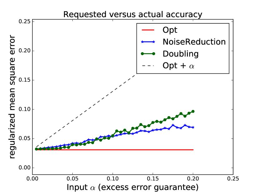
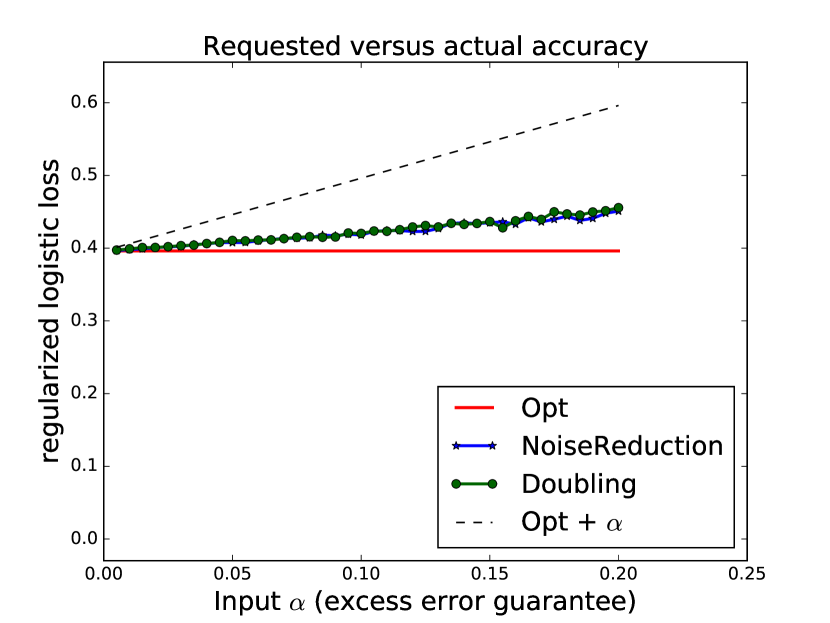
Refer to caption
(a) Linear (ridge) regression.
Refer to caption
(b) Regularized logistic regression.
Refer to caption
(c) Linear (ridge) regression.
Refer to caption
(d) Regularized logistic regression.
Figure 2: Empirical accuracies. The dashed line shows the requested accuracy level, while the others plot the actual accuracy achieved. Due most likely due to a pessimistic analysis and the need to set a small testing threshold, accuracies are significantly better than requested for both methods.
Refer to caption
(a) Linear (ridge) regression.
Refer to caption
(b) Regularized logistic regression.
Figure 3: Privacy breakdowns. Shows the amount of empirical privacy loss due to computing the hypotheses themselves and the losses due to testing their accuracies.
Refer to caption
(a) Linear (ridge) regression.
Refer to caption
(b) Regularized logistic regression.
Figure 4: L2subscript𝐿2L_{2} norms of final hypotheses. Shows the average L2subscript𝐿2L_{2} norm of the output θ^^𝜃\hat{\theta} for each method, versus the theoretical maximum of 1/λ1𝜆1/\sqrt{\lambda} in the case of ridge regression and 2log(2)/λ22𝜆\sqrt{2\log(2)/\lambda} in the case of regularized logistic regression.

B.3 Supporting theory

Claim B.1.

For the “doubling method”, the factor 222 increase in ε𝜀\varepsilon at each time step gives the optimal worst case ex post privacy loss guarantee.

Proof.

In a given setting, suppose εsuperscript𝜀\varepsilon^{*} is the “final” level of privacy at which the algorithm would halt. With a factor 1/r1𝑟1/r increase for r<1𝑟1r<1, the final loss may be as large as ε/rsuperscript𝜀𝑟\varepsilon^{*}/r. The total loss is the sum of that loss and all previous losses, i.e. if t𝑡t steps were taken:

(ε/r)+r(ε/r)++rt1(ε/r)superscript𝜀𝑟𝑟superscript𝜀𝑟superscript𝑟𝑡1superscript𝜀𝑟\displaystyle(\varepsilon^{*}/r)+r\cdot(\varepsilon^{*}/r)+\dots+r^{t-1}\cdot(\varepsilon^{*}/r) =(ε/r)j=0t1rjabsentsuperscript𝜀𝑟superscriptsubscript𝑗0𝑡1superscript𝑟𝑗\displaystyle=(\varepsilon^{*}/r)\sum_{j=0}^{t-1}r^{j}
(ε/r)j=0rjabsentsuperscript𝜀𝑟superscriptsubscript𝑗0superscript𝑟𝑗\displaystyle\to(\varepsilon^{*}/r)\sum_{j=0}^{\infty}r^{j}
=εr(1r)absentsuperscript𝜀𝑟1𝑟\displaystyle=\frac{\varepsilon^{*}}{r(1-r)}
4ε.absent4superscript𝜀\displaystyle\geq 4\varepsilon^{*}.

The final inequality implies that setting r=0.5𝑟0.5r=0.5 and (1/r)=21𝑟2(1/r)=2 is optimal. The asymptotic \to is justified by noting that the starting ε1subscript𝜀1\varepsilon_{1} may be chosen arbitrarily small, so there exist parameters that exceed the value of that summation for any finite t𝑡t; and the summation limits to 11r11𝑟\frac{1}{1-r} as t𝑡t\to\infty. ∎