The evaporation valley in the Kepler planets
Abstract
A new piece of evidence supporting the photoevaporation-driven evolution model for low-mass, close-in exoplanets was recently presented by the California-Kepler-Survey. The radius distribution of the Kepler planets is shown to be bimodal, with a “valley’ separating two peaks at and R⊕. Such an “evaporation-valley’ had been predicted by numerical models previously. Here, we develop a minimal model to demonstrate that this valley results from the following fact: the timescale for envelope erosion is the longest for those planets with hydrogen/helium-rich envelopes that, while only a few percent in weight, double its radius. The timescale falls for envelopes lighter than this because the planet’s radius remains largely constant for tenuous envelopes. The timescale also drops for heavier envelopes because the planet swells up faster than the addition of envelope mass. Photoevaporation therefore herds planets into either bare cores (), or those with double the core’s radius (). This process mostly occurs during the first Myrs when the stars’ high energy flux are high and nearly constant. The observed radius distribution further requires that the Kepler planets are clustered around in mass, are born with H/He envelopes more than a few percent in mass, and that their cores are similar to the Earth in composition. Such envelopes must have been accreted before the dispersal of the gas disks, while the core composition indicates formation inside the ice-line. Lastly, the photoevaporation model fails to account for bare planets beyond days, if these planets are abundant, they may point to a significant second channel for planet formation, resembling the Solar-System terrestrial planets.
Subject headings:
planets and satellites: atmospheres — planets and satellites: composition — planets and satellites: formation — planets and satellites: physical evolution1. Introduction
Recent exoplanet discovery missions and targeted follow-up campaigns have fundamentally changed our understanding of what constitutes a “typical” planet (e.g. Borucki et al., 2011; Marcy et al., 2014). Specifically, the most common type of exoplanets are smaller than Neptune (4 R⊕, e.g., Youdin 2011; Howard et al. 2012; Batalha et al. 2013; Petigura et al. 2013; Burke et al. 2014; Morton et al. 2016) and have masses of a few to tens of Earth masses. The fraction of sun-like stars that host at least one of these “Kepler” planets with an orbital period of less than 100 days is around 60–90% (e.g. Fressin et al., 2013; Silburt et al., 2015; Mulders et al., 2016).
Combining transit measurements of a planet’s radius with a measurement of its mass from transit-timing variations (TTVs, Carter et al. 2012; Wu & Lithwick 2013; Hadden & Lithwick 2014; Jontof-Hutter et al. 2016; Hadden & Lithwick 2016) or radial-velocity (RV) follow-up (e.g. Marcy et al., 2014; Weiss & Marcy, 2014) quickly told us that many of these planets had compositions unlike the small terrestrial planets in our own solar system (e.g. Wolfgang et al., 2016). Rather than being completely solid, such planets are likely to be composed of a dense solid core surrounded by a voluminous volatile rich envelope. However, due to degeneracies present in the mass-radius plane at low-masses (e.g. Adams et al., 2008; Rogers & Seager, 2010), we cannot infer the compositions just based on the current measured mass and radius for the majority of the observed planets. These degeneracies can be broken by considering how the local environment effects the evolution of the planet. For example, Wu & Lithwick (2013) showed that closer-in planets tend to be denser, while Ciardi et al. (2013) demonstrated that for pairs of planets in multi-planet systems, the inner planet tends to be smaller. These studies suggest that the envelopes are rich in hydrogen/helium.
Orbiting close to their parent stars, the Kepler planets can receive, over a lifetime, an integrated high-energy irradiation (high-energy exposure) that is an appreciable fraction of their gravitational binding energy (e.g. Lammer et al., 2003; Lecavelier Des Etangs, 2007; Davis & Wheatley, 2009), where this high-energy “exposure” is dominated by the first Myr of the planet’s lifetime (e.g. Jackson et al., 2012). Planets with H/He-rich envelopes can be strongly evaporated by this irradiation (e.g. Yelle, 2004; Tian et al., 2005; Murray-Clay et al., 2009; Owen & Jackson, 2012; Johnstone et al., 2015; Erkaev et al., 2016), and indeed H/He evaporation has been observed from the low-mass planet GJ 436b (Kulow et al., 2014; Ehrenreich et al., 2015). Evaporation naturally results in planets that are smaller and denser than those at large separations (e.g. Lopez et al., 2012; Owen & Wu, 2013; Lopez & Fortney, 2013; Jin et al., 2014; Howe & Burrows, 2015). For a planet with a low enough mass and a close enough orbit, its initial low-mass H/He envelope can even be entirely stripped, leaving behind a naked solid core. This explains the dearth of planets with any envelopes at short periods (Lundkvist et al., 2016). The core’s mass and density play a primary role in controlling a planet’s evolution by setting the escape velocity (Owen & Wu, 2013; Lopez & Fortney, 2013; Owen & Morton, 2016; Zahnle & Catling, 2017), allowing one to break the compositional degeneracies in individual systems by statistical modelling (Owen & Morton, 2016). While steam atmospheres are also expected to lose mass (as in the case of early Venus – Kasting & Pollack 1983) the evaporative histories of such planets are significantly different to those that contain H/He envelopes and therefore distinguishable (Lopez, 2016).
While the evaporation theory naturally explains why Kepler planets are larger and less dense further out, it also makes another major prediction: the existence of an “evaporation valley”, a low-residence region in the radius-period plane between planets that have been completely stripped and those that are able to retain an envelope with roughly % in mass. The evaporation valley was first predicted by Owen & Wu (2013) using numerical evolutionary studies for low-mass planets with pure rock (silicate) cores, and shortly after, by Lopez & Fortney (2013) for different core compositions using a different evaporation model. The evaporation valley was further reproduced by Jin et al. (2014) and Chen & Rogers (2016), again using different evaporation prescriptions and initial populations. The evaporation valley is thus a robust prediction of evaporative driven evolution of close-in H/He rich planets. This feature is largely independent of the assumed H/He evaporation model (energy-limited, recombination limited, UV driven, X-ray driven etc.), and its creation also appears insensitive to the choice of initial conditions (for at least a reasonable range of starting conditions); however, the details of these choices do control it’s properties (width, location with orbital period etc.).
The predicted occurrence valley, between stripped cores and those that retain a residual H/He envelope, is not particularly wide, with a radius width of R⊕ (see Fig. 8 of Owen & Wu 2013 and Fig. 9 of Lopez & Fortney 2013). Large planetary radius errors, stemming from uncertainties in the stellar radius, have previously hampered efforts to observationally solidify its presence in the observed exoplanet population (see Owen & Wu, 2013, for a preliminary analysis that suggested its presence). Recently, the California-Kepler Survey (CKS), using spectroscopic follow-up of a large (1305) sample of planet hosting Kepler stars (Petigura et al., 2017) refined the planet parameters for 2025 Kepler planets, and reduced the typical planetary radius error to % (Johnson et al., 2017). The CKS sample allowed Fulton et al. (2017) to definitely reveal a valley in the planet occurrence rate in the planet radius – period plane: close-in planets predominantly have a radius of either R⊕ or R⊕, while planets with a radius of R⊕ are considerably rarer, in spectacular agreement with the predicted evaporation driven evolution scenario for close-in exoplanets (Owen & Wu, 2013; Lopez & Fortney, 2013; Jin et al., 2014; Chen & Rogers, 2016).
While the presence of the evaporation valley in numerical models is robust to changes in model assumptions, a clear physical, first-principle description of its origin is missing, along with an understanding of how its properties change with model assumptions such as the core composition and evaporation model, and even when or whether it could be made to disappear. This paper serves two purposes: firstly, we clearly explain the physics behind the origin of the evaporation-valley; secondly, we will perform a preliminary investigation into how the observed evaporation valley can break many of the composition degeneracies and make inferences about both the composition of the Kepler planets and how/where they formed.
2. A minimal analytical model
Here, we build a minimal model of an evolving planet under the influence of evaporation and cooling. The planet is assumed to consist of a solid core of mass , and radius , surrounded by a gaseous envelope whose equation of state can be described by the ideal gas law. Such a model allows us to determine the planet outer radius as a function of time and envelope mass. We then perform numerical checks to confirm these results. While a fully numerical study is straight-forward (and has been done), such an approach obscurates the underlying properties of low-mass exoplanet atmospheres that results in the evaporation valley. Furthermore, the analytical method sheds light on many of the parameter dependencies.
2.1. Radius versus envelope mass for a low-mass planet
Our goal here is to understand how the radius of the planet () changes with its envelope mass fraction () with a view to calculating the mass-loss timescale. We consider low-mass envelopes (), so the planet’s mass is still dominated by the core. Therefore, we neglect the self-gravity of the planet’s envelope.111The role of self-gravity is to compress the envelope giving it a smaller radius than our following analysis predicts. Self-gravity becomes important when and larger, and its impact is demonstrated in Fig 1.
Due to stellar insolation, the envelope is adiabatic (convective) in the deep interior and roughly isothermal (and radiative) near the surface. The roughly isothermal radiative cap satisfies (e.g. Rafikov, 2006; Lee & Chiang, 2015; Ginzburg et al., 2016), where the photospheric equilibrium temperature is set by stellar insolation. The radiative-convective boundary is assumed to occur at a density , and a radius . The planet’s radius is set by the photospheric radius and is typically pressure scale heights above (see also Lopez & Fortney, 2014), where the scale height in the isothermal layer is,
| (1) | |||||
where we have estimated its value for a Sun-like host (mass 1 M⊙, radius 1 R⊙ and effective temperature 5780 K) and for an envelope with a mean-molecular weight of (solar composition), surrounding a core with an earth-like composition (see eq. 15). So the isothermal radiative cap is geometrically thin. In the following derivation, we take the planet radius to be approximately , but correct for the isothermal layer thickness in all relevant places (including all figures).
2.1.1 Convective interior
Adopting an equation of state for the adiabatic part of with and being constants,222In reality, for our ideal gas envelope transitions from in the upper envelope where molecules dominate to in the lower envelope where molecules are dissociated. But the bulk of the planet can be considered as atomic. hydrostatic equilibrium gives a density profile of:
| (2) |
where is the adiabatic gradient, and the isothermal sound speed is evaluated at . For planetary atmospheres that are strongly bound ()333Even if the initial planets may not be so, they rapidly evolve to such a state via the “boil-off” process investigated in Owen & Wu (2016)., the unity term inside the braket can be safely ignored for much of the planetary interior that contributes significantly to the envelope mass, and we can simplify the above expression into
| (3) |
Solving for the mass enclosed in the atmosphere yields:
| (4) | |||||
where the dimensionless integral is:
| (5) |
The properties of this dimensionless integral are discussed in the appendix. For , as applies for the bulk of the atomic interior, the integrand for peaks at . So in the limit of a puffy envelope, , is fairly independent of and is of order unity. While in the opposite limit of a thin envelope, quantified as , the integral can be approximated as
| (6) |
With these expressions, the envelope mass fraction can be expressed as a function of the envelope thickness, , in the two regions and :
| (7) | |||||
where we have dropped all order unity constants for clarity.
While the above expression relates to , it still contains a variable that depends on planet radius and envelope mass, among other things. To eliminate these dependencies, we appeal to the characteristics of the radiative-convective boundary. At this location, the temperature gradient remains adiabatic by definition, or , giving rise to,
| (8) |
The mode of energy transport changes at this point from advection by convective eddies to radiative diffusion, allowing us to write
| (9) |
where we have approximated values for the temperature and radius at the radiative-convective boundary as those at the surface, the impact of this approximation is discussed in § 3.4. The internal luminosity arises from gravitational contraction of the atmosphere, i.e., changes in the gravitational binding energy ,444We ignore other internal heat sources, e.g., the heat capacity of the core and energy from radioactive decay. See discussion in § 4.3.
| (10) |
Using eqs. (2) & (4), we can re-write the luminosity as
| (11) |
where is the Kelvin-Helmholtz timescale (or cooling timescale). It is of order the planet age except in two cases: pre-cooling (the case considered in Owen & Wu, 2016) and high mass-loss rate (see §3.4). is another dimensionless integral given by
| (12) |
whose relation to is discussed in the appendix. It is also shown there that the ratio smoothly varies from to over the parameter range of interest. Finally, we adopt an opacity law of to obtain the following expression for the density at the radiative convective boundary, by substituting eqs. (8) & (11) into eq. (9),
| (13) |
Substituting this into eq. (7), we obtain the final monotonic dependence of envelope mass fraction on planet radius of
| (14) | |||||
where we have dropped all constants of physics and assumed that, due to compression, all solid cores (naked planets) have mass-radius relation as (Lopez & Fortney 2014, following, Fortney et al. 2007, Valencia et al. 2010), or
| (15) |
where is the density of a 1 M⊕ core and depends only on the core composition. For terrestrial composition, , while it is , and g cm-3 for pure iron, silicate and water/ice cores respectively (Fortney et al., 2007). The power indexes are, respectively,
| (16) |
where we have also evaluated these expressions with , , , the latter two identified by Rogers & Seager (2010) as the opacity law appropriate for a solar metalicity H/He envelope of a low-mass, highly irradiated planet (also see Freedman et al., 2008).
So, at a given planet size (), the exponents in eq. (16) tell us the envelope mass is higher for a denser core composition (e.g., iron oxide vs. water ice), for an older planet, and for planets further away from their stars, all as expected. Furthermore, the nature of the opacity law makes the planet size a direct measure of the H/He envelope mass fraction, with weak sensitivities to all other factors. This has been noticed numerically in earlier works (e.g., Lopez & Fortney, 2014; Chen & Rogers, 2016). Lopez & Fortney (2014) provide power-law fits to their numerical models over a wide range of parameter space, and the power-law indices listed in eq. (16) are similar to their results (eq. 4 in that paper, though theirs are fits for an “enhanced opacity” model, not solar-metallicity). A different opacity law may lead to very different results.
Now, let us define an value at which the planet radius doubles, , as . We shall argue later that is a crucial parameter for producing the evaporation valley. In eq. (14), setting and re-inserting all constants that we have previously suppressed (with cm2 g-1 at a pressure of 1 bar and a temperature of 1000 K, Rogers & Seager 2010), and for solar metallicity gas, we find:
| (17) | |||||
where is the orbital period. We have also set and adopted an empirical mass-luminosity relation for low-mass dwarfs: (see, e.g. Cox, 2000). In principle, the value of also depends on . But since it varies by only a factor of within our range of interest, together with the weak index , this can be safely ignored. Moreover, when the thickness of the isothermal layer is accounted for, the true is slightly smaller. We actually obtain that is of order a few percent at an age of a Gyrs.
In summary, the envelope mass fraction, at which the planet’s radius doubles, is of order a few percent, and is a relatively weak function of planet period, stellar mass, core mass and planet age.
2.2. Timescale for atmospheric erosion
We define a mass-loss timescale for envelope evaporation as
| (18) |
In the following, we show that this timescale naturally peaks for envelopes with masses , or those which double the core’s radius.
The mass-loss rate is given by the ratio of photo-evaporative power and the binding energy of the planet (Lecavelier Des Etangs, 2007; Erkaev et al., 2007). Let be the luminosity of high energy photons from the star, and the dimensionless factor be the efficiency of these photons for mass-removal,555This efficiency is defined as if the high-energy photons are intersected by a cross-section . The definition of this efficiency is arbitrary and many other definitions do exist in the literature. the mass-loss rate is
| (19) |
The efficiency factor is not necessarily a constant, as has been demonstrated in multiple works (e.g. Murray-Clay et al., 2009; Owen & Jackson, 2012; Shematovich et al., 2014; Owen & Alvarez, 2016; Salz et al., 2016). However, when compared to full radiation-hydrodynamic models it takes a value of order for low-mass planets (Owen & Jackson, 2012; Owen & Alvarez, 2016). For simplicity, we adopt a constant (the so-called “energy-limited” approach, see e.g., Lopez & Fortney, 2013). However, we discuss its variation and impact on the planet population in §4.5. We do not consider an “effective absorption radius” or “expansion radius” (e.g. Baraffe et al., 2004) that accounts for the higher radius at which the high-energy flux is absorbed compared to the planet’s radius, as this effect can always be folded into the efficiency factor. Such a radius is also difficult to define for X-ray driven evaporation (which is important for low-mass planets) as different wavelength photons can be absorbed at very different radii. We also neglect the effect of stellar tides (e.g. Erkaev et al., 2007) since most observed planets are far from their Roche radii. Specifically of the planets (taking them to have a mass of 3 M⊕) used in the Fulton et al. (2017) sample would have their mass-loss rates increased by and would have their mass-loss rates increased by a factor of using the (Erkaev et al., 2007) prescription.
Substituting eq. (14) into the above expressions, we obtain:
| (20) | |||||
where we evaluate for solar-metallicity gas, and have adopted a parameter to account for the difference between and the photospheric radius, . In our model, is computed self-consistently, by locating the photosphere at where . The photosphere radius is then at above the radiative-convective boundary, with being the local scale height, and , where is the density at the photosphere.
According to eq. (20), the mass-loss timescale reaches a maximum at the point at which the radius is doubled (, ). Such a behaviour arises because, below , the planet’s radius is dominated by that of the core and is independent of the envelope mass. So the photoevaporation timescale decreases for lower envelopes. This is an unstable situation that can cause complete stripping. While above , increasing leads to a radius expansion. The expansion is so significant that, for our adopted opacity laws and a constant , the evaporation timescale shortens. This behaviour can be shown to occur for all well known evaporation models: energy-limited evaporation, when the radius increases faster than ; photon-limited evaporation (Owen & Alvarez, 2016), where the radius increases faster than ; and recombination limited evaporation (Murray-Clay et al., 2009), where the mass-loss rate is exponentially sensitive to radius (Owen & Alvarez, 2016) such that the erosion time-scale always decreases with increasing envelope mass fraction. The fact that the envelope-mass loss time scale peaks for low-mass planets with envelope mass fractions of order a few percent was also noticed numerically by Chen & Rogers (2016) using mesa models. With our minimal model, it becomes obvious that the mass-loss timescale always peaks around . For this feature not to happen, one requires , or in terms of the opacity scaling with pressure, , which is unrealistic.
The heuristically derived eq. (20) has a sharp discontinuity at . Numerically, we smooth the transition in the preceding calculations by using the fact, in reality , rather than the approximation for and for , presented above.
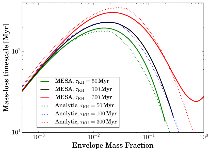
In the following, we will construct planetary structure models, based on eqs. (4), (11) and (13). In Fig. 1, we compare results from our minimal models against those produced using the mesa code (Paxton et al., 2011, 2013, 2015), suitably modified for highly irradiated low-mass planets (see Owen & Wu, 2013; Owen & Morton, 2016). The agreement between the analytic model and the mesa results is good. The mass-loss timescale peaks at , roughly where the planet doubles in size, increases slowly with cooling time; and the mass-loss timescale falls off as predicted on both sides of the peak. The agreement only fails for cases where , where the self-gravity of the envelope (ignored in our analytical models) becomes dominant. At large envelope masses, self-gravity keeps the planet’s radius roughly constant to of order a Jupiter radius, and the mass-loss time begins to increase again as expected (it is well known hot jupiters are stable to evaporation, e.g. Yelle 2004).
3. Comparing to the observations – the “evaporation valley”
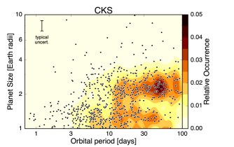
Based on refined stellar parameters from the CKS survey, Fulton et al. (2017) reported a “gap” in the planetary radius distribution (also noticed by Owen & Wu, 2013, based on the cruder KIC data): a deficit of planets at radii (“gap”) that appears to extend from 10 days to 100 days in orbital period (“valley”). We now use our analytical model to calculate the exact valley location for different parameters. In the following, we detail our model choices and present results.
We make no effort to “fit” the observations at this stage, especially with our minimal model. That is best left to comparisons with numerical models. Nevertheless, as we will see, even our model can be used to make strong inferences about the properties and possible formation channels of the Kepler planets. Usefully, we can analytically understand the origin of these constraints.
3.1. The Integration
Starting from an initial envelope mass fraction at time zero, which we set to be 1 Myr (roughly the disk dispersal timescale, e.g. Hernández et al., 2007), we evolve the envelope mass fraction according to:
| (21) |
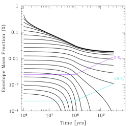
according to eq. (20), and a prescription for the stellar high energy luminosity (§3.2), and the cooling of the planet (§3.3). Some example evolutionary tracks for a planet with different initial envelope mass fractions is shown in Fig. 2.
We have also applied our analytical model to the envelope evolution of the Kepler-36b/c system and compare them against the more detailed mesa calculations presented in Owen & Morton (2016). We find that while we can reproduce their general results, namely, the lower mass Kepler-36b is completely stripped off, while the higher mass Kepler-36c retains a bulky envelope, our models suffer moderately more mass loss for the latter planet during the early stages when its mass-loss rate is high, due to our assumption of constant mass-loss efficiency, an assumption not adopted by Owen & Morton (2016).
3.2. Stellar Parameters
We adopt host star masses similar to those in the CKS sample (Fulton et al., 2017), a Gaussian distribution in mass, centred at with a variance of .
For the magnitude and the evolution of the high-energy flux (, including UV through X-ray radiation), we adopt the empirical relation for main-sequence dwarfs, as summarized by Jackson et al. (2012)
| (22) |
We further choose and Myrs, and , motivated by the body of observational and modelling works (e.g. Güdel et al., 1997; Ribas et al., 2005; Jackson et al., 2012; Tu et al., 2015). Since , the time-integrated high-energy “exposure” (Lecavelier Des Etangs, 2007; Jackson et al., 2012; Owen & Wu, 2013) is dominated by that in the first Myrs. So the exact choice of has little bearing on the final planet properties.
3.3. The Planet Ensemble
We now must decide what the primordial Kepler planets look like. In this work, we consider only one population of planets – we discuss the evidence for a second population in §4.7.
We adopt the following orbital period distribution for planets around all stars,
| (23) |
This distribution is obtained by fitting the Kepler planet sample and correcting for transit probabilities. It is similar to those obtained in earlier work (e.g. Fressin et al., 2013).
For the planetary cores, we assume them to be Earth-like (). In §4.2, we will vary this parameter and show that the observed CKS sample actually demands this choice. Furthermore, we take a Rayleigh distribution for the core mass
| (24) |
The actual mass distribution of Kepler planets has not been reliably established. Early RV studies (e.g. Howard et al., 2010; Mayor et al., 2011) showed that the planet occurrence rate increased towards low-masses: planets in the mass range 3-10 M⊕ being most common, with the occurrence rate falling rapidly towards higher masses. One more recent attempt is provided by Marcy et al. (2014) where they selected 22 KOIs and measured masses (or their upper-limits) for 42 planets. The mass function for this group can roughly be fit as a Rayleigh distribution with a mode M⊕. However, this sample is arguably biased towards higher masses – compared to Kepler planets within the same period range (say, days), this sample contains planets that are, on average, larger and therefore likely more massive. We therefore choose a slightly smaller mass scale of M⊕. We are also motivated by the position of the small-size peak. At a radius of R⊕, this corresponds to a terrestrial planet with M⊕.
We also need to prescribe the initial envelopes. This includes both their initial thermal time (which determines the initial entropy) and initial masses. Owen & Wu (2016) argued that after low-mass planets are born, they undergo a rapid phase of cooling and mass-loss (the “boil-off” phase) and age prematurely to Myrs within a relatively short time. After about 100Myrs, they continue to cool off normally. So we take
| (25) |
Due to the fact and the above form of cooling contraction, most of the envelope erosion occurs in the first 100 Myrs, and there is little change to the planet atmosphere after that.
To guide our choice for the initial envelope mass, we first ask what kind of planets would have occupied the observed gap, at an age of a few billion years. These are the grey points in Fig. 3, for cores of terrestrial composition (), with a range of core mass, initial envelope mass, and orbital period. Since these models would appear in the CKS gap, they are disfavoured by the observations. Now we make the important assumption that planets are born with the same envelope mass and core mass distributions across the range of period of interest (from a few to days). This assumption mostly reflects our ignorance on the proper initial condition, and is almost certainly not true in reality. But under this restrictive assumption, all models that are marked with grey in the right-hand panel of Fig. 3 are not permitted. In other words, there are two groups of planets that are likely progenitors for the observed Kepler planets: one group are planets that are slightly more massive ( M⊕) and are born with at least a few percent of H/He; the other group, planets that are less massive ( M⊕) and that are born, for all purposes, bare. The second group cannot account for planets with radii larger than R⊕. Furthermore, Fulton et al. (2017) indicate that the completeness of their exoplanet radius distribution becomes uncertain at small planet radii R⊕. Inspection of Fig 3 indicates that planets with masses M⊕ ( R⊕) are disfavoured if they contain H/He envelopes with masses of a few percent or more. Therefore, while the current CKS sample cannot determine if planet occurrence drops significantly below 1.14 R⊕ we predict it should, unless there is a second population of planets (see §4.7). Moreover, we emphasize that the choice of the mass scale, M⊕, is motivated by both the radii of the bare planets, and the size distribution of planets to the right of the valley.
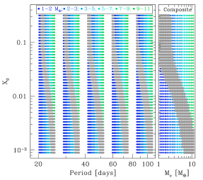
Guided by this insight, we adopt a logarithmically flat distribution for , the initial envelope fraction, with and and . The value of matters little as long as it lies well above , while the value of is suggested by Fig. 3, for our choice of core masses.
3.4. A few details
The radius measured for a planet by the transit method is not the photospheric radius (which accounts for the radial light-path for the local black-body photons), but should be determined by the tangent light-path for transmitting stellar photons. The chord is longer for the latter group by a factor of , increasing the transit radius by (e.g. Lopez & Fortney, 2014). However, opacity for optical photons is smaller than that for infra-red photons, leading to a “deeper photosphere”. These two effects cancel each other to some degree and we decide to ignore them here.
Another complication arises from how we treat the thermal evolution of the planet in presence of mass-loss. Here, we simply assume the two are independent (eq. 25). This is inappropriate when the envelope is being evaporated faster than cooling contraction. In this case, the lifting of pressure at the top allows the envelope to expand adiabatically. The irradiated atmosphere then actually transports heat inward, maintaining the same internal entropy. The radiative-convective boundary remains fixed at the same density, and the internal entropy can be transported out with the same cooling luminosity as before. This accelerates the cooling compared to the case of no-cooling (this is the physical basis for the “boil-off” discussed in Owen & Wu 2016, see also the discussion in Ginzburg et al. 2016). We do not correct for this effect in our minimal model, but note that this may lead to enhanced mass loss in some cases; however, models that typically enter this region are on their way to be completely stripped anyway.
3.5. Planets at a few Gyrs
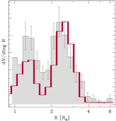

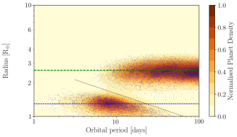
We evolve our initial population for three billion years under the influence of cooling and evaporation. The resulting radius distribution for planets with orbital periods less than 100 days is presented in Fig. 4. Compared to the observed 1-D radius distribution from the CKS sample, our model reproduces the observed features: the positions of the radius gap and the radius peaks, the widths of the peaks. More significantly, the observed valley in the radius-period 2-D plane is reproduced nicely by our model. This is shown in Fig. 5, alongside with the observed results by Fulton et al. (2017). Both these successes strongly support the photoevaporation theory for the evolution of Kepler planets.
Since we have not attempted to “fit” the observed distribution, but rather to match its generic features, the agreements are not perfect. Short of theoretical predictions for the initial planet properties (how they depend on, e.g., separation, stellar mass, planet core mass, etc.), and only using an approximate photoevaporation model (the energy-limited case), this not surprising. In future work, using numerical models, one may actually be able to use the observed planet population to infer these initial properties. In the following, we discuss what parameters change may impact on the agreements.
4. Discussion
We have used an analytic model to demonstrate that the evaporation valley is a robust outcome of the evolution of close-in, low mass planets with volatile envelopes. The mass-loss timescale always peaks for a H/He envelope of a few percent in mass, where the atmosphere roughly doubles the planet’s radius (see also Chen & Rogers, 2016). This simple combination of planetary structure and evaporation is the origin of the bimodal radius distribution reported in Fulton et al. (2017). Here, we explain these results in more depth, and investigate impacts on our model from various model uncertainties.
4.1. The origin of the evaporation valley
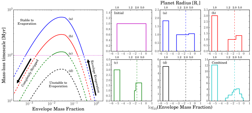
The origin for the evaporation valley is schematically shown in Fig. 6. Consider a group of identical, low-mass planets differing only in their initial envelope mass fractions () and high-energy exposure. Since after the first 100 Myrs, both the stellar flux decays and the planet cools down to a smaller size, the evaporation is dominated by that in the early stages. For a group of planets with the same high-energy exposure, if the peak mass-loss timescale – for – is shorter than 100 Myrs (model d in Fig. 6), all envelopes are stripped bare and we expect to see only naked cores, as is the case for the observed Kepler planets at small separations (e.g. Dressing et al., 2015). If, on the other hand, the peak mass-loss timescale is longer than Myrs (group c in Fig. 6), there is a bifurcation of final envelope masses – planets with initial envelope masses will be completely stripped and present as naked cores; while planets with initial will be herded towards . This manifests as a bifurcation in planet radius, with peaks at both the core size and its double. This bifurcation is the origin of the evaporation valley.
Lastly, for planets in group a and b which experience too little evaporation, there are little modifications to their atmospheres unless they start with extreme envelope masses (very high or very low). There is still a shepherding toward the above mentioned two peaks, but the widths of the second peak (at twice the core radius) are broader. The observed valley shape can then be used to exclude some of these models, as is done in Fig. 3, where we show that most of the initial envelopes should have more than a few percent in mass.
This understanding allows us to derive some useful scalings. These are detailed here and below.
Since less massive planets can be stripped out to larger distances, the bare population should have a decreasing size (smaller mass and hence smaller core radius) going away from the star. We can derive this by requiring that, for a given core mass, the longest evaporation time (when , or ) is of order or 100 Myr,
| (26) |
or,
| (27) |
where is the high-energy “exposure” for a given planet. Then combining eq. (15) & (17), we can find the radius of the most massive planet that can be stripped () at a given exposure as:
| (28) |
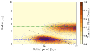
Using the high-energy flux dependence on stellar mass (§3.2), , as well as eq. (14), we convert the above relation to find , shown as the dotted black line in the left hand panel of Fig. 5. This explains the topology of the evaporation valley in the radius-period plane, in models with a constant evaporation efficiency . As we discuss later, this scaling can change when the evaporation model is different, while the core composition can shift the black line vertically.
4.2. Core Composition
When the evaporation valley was first predicted by Owen & Wu (2013); Lopez & Fortney (2013) and subsequently by Jin et al. (2014), its location was conjectured to be a discriminant of core composition which could provide clues as to their formation (Lopez & Rice, 2016). And indeed our model shows clear dependency on the core composition.
Following our discussion above, we posit that the valley, independent of the core composition, always lies in-between and . Let us say, . Or
| (29) |
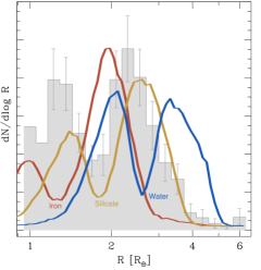
This is demonstrated in Fig. 7, where cores of the same mass but different composition exhibit different valleys. An order of magnitude in change in leads to an easily detectable shift in the valley position of a factor 2, much larger than the radius errors achieved in the CKS sample (Johnson et al., 2017), and even large compared to the error in the general Kepler sample. So if the planet mean masses are known, the valley position yields the core composition.
Interestingly, even when the planet mean masses are not known, if we assume the bimodal radius distribution arises from a single population of planets, we can break the degeneracy and determine the composition. In our model, we successfully reproduce the observed valley using a single population of planets with (see also §4.7) and terrestrial compositions. This does not seem possible for some other compositions. For instance, if the cores are made up largely of ice/water with , the bare cores at will correspond to , and none of these cores can retain enough hydrogen to occupy the second radius peak. Similarly, for pure iron composition (), the bare cores should correspond to . However, few of these planets could be evaporated down to naked cores, at the distances that we observe them. So the current data exclude cores that are mostly icy, and favour compositions that are terrestrial-like, i.e., silicate-iron composite. This is consistent with RV results from known bare planets (e.g. Dressing et al., 2015).
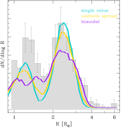
While these cores are Earth-like, we find that we cannot constrain their iron fractions to a narrow range using current data: in Fig. 8, we present the expected size distributions for different iron fractions, and all appear largely consistent with data. This could reflect either a genuine composition spread in real planets, or an intrinsically narrow composition spread that is smeared out by errors in the observed data.
In conclusion, the observed gap suggests that the most common core composition is Earth-like. But the iron fractions in these silicate-iron composite could span a wide range; with a detailed numerical fit to the observed population one maybe able to constrain the Iron fraction to a narrower range.
4.3. Core Luminosity
For simplicity, in the main analysis, we have ignored the luminosity contribution from the cooling core. This is not justified in general, since the thermal content in the more massive core can be more substantial than that in the envelope. We address this deficiency here.
We assume that the entire planet, core and atmosphere, cools with a single temperature. This is reasonably accurate for the solid interior, since even the adiabatic temperature gradient is relatively shallow. For an envelope with , () the thermal inertia is dominated by gas in the bottom few scale heights close to the core. Gas here likely share the same temperature as the solid part. We further assume that the core contributes only through its primordial heat, and ignore any radiogenic source. This is valid, especially at early times. For the heat content of the core, we adopt a heat capacity of erg g-1 K-1 (Valencia et al., 2010, similar to rock), and we assume that the core is made up of SiO2 molecules with a mean molecular weight of (or per particle specific heat of ). The envelope is assumed to be composed of H-atoms with a per particle specific heat of . So including the core contribution to the internal luminosity, we have
| (30) | |||||
This expression explains the results shown in Fig. 3 of Lopez & Fortney (2014). We insert this factor into eq. (11) and re-calculate the photo-evaporation process. Core luminosity allows the adiabatic envelope to remain large for a longer time, enhancing mass-loss. However, the overall effect is minor. This is because the evaporation bottleneck is when the envelope mass fraction is of order a few percent (). At this point, the core contribution to the luminosity is an order unity effect.
4.4. Atmosphere Metallicity
Some studies of transmission spectroscopy have suggested that the atmospheres of hot Neptunes (e.g., GJ1214b) are highly enriched in metals, with [Z/H] perhaps as high as 100 (e.g. Charnay et al., 2015), while others (e.g. HAT-P-26b) are consistent with solar metallicity (Wakeford et al., 2017) . Here we explore how atmosphere metallicity may affect our results.
Metallicity enters our model in two ways (eq. 14). First, higher metallicity increases the mean molecular weight (), which reduces the scale height at a given temperature. This shrinks the atmosphere, and increases the value of . Second, higher metallicity increases opacity (), which shifts the convective-radiative boundary. Thus, the atmosphere looks more inflated for a given age. The outcome of our model is determined by the competition between these two effects (also see Howe & Burrows, 2015). Reality may be more complicated. The constant energy-efficiency approach we adopt here may be severely invalid if metals affect the driving of the photo-evaporative flow.666For X-ray driven flow, metals (like C, O) dominate both the absorption of X-ray photons and the line cooling of the heated region (Owen & Jackson, 2012). The two effects may cancel out to a large degree. For EUV driven flow, hydrogen photo-ionization and recombination dominate the heating and cooling, though metals, if present at a large quantity, may reduce the energy efficiency as additional sources of radiative cooling. Metals may have additional thermal effects by, for instance, producing high altitude hazes/clouds.
Assuming that (e.g. Lee & Chiang, 2015), we find that, overall, raising the metallicity leads to a slightly larger radius and hence a slightly shorter mass-loss timescale. The effect maximizes (making a factor of 2 difference in timescale) when the metallicity is solar, but nearly vanishes when it is solar. Such an effect is so small it is eclipsed by other uncertainties in our current model. As a result, we can not make conclusive statement regarding atmosphere metallicity, aside from the fact that the initial atmosphere must be dominated by H/He in number (and so in molecular weight). For example, the observed position in the radius-period plane rules out the presence of “water-worlds” whose volatile envelopes are primarily water/steam. Water/steam atmospheres have a much larger mean-molecular weight () compared to H/He envelopes, this significantly increases the value of to values more like (Lopez, 2016). The increased high-energy exposure required to evaporate an envelope with (even with an optimistic efficiency of 0.1 for steam atmospheres) results in the evaporation valley appearing at much shorter separations, around a period of 2 days (Lopez, 2016), rather than the 10 days it is observed. Therefore, water-worlds making up any reasonable fraction of the Kepler planets is clearly ruled out by the CKS observations.
4.5. Evaporation Efficiency
There are two reasons why the evaporation efficiency may not be constant for all planets. First, geometry. We define the efficiency to be based on the light received by the planet disk (). However, the true cross-section is determined the UV/X-ray photosphere. This lies well above the planet photosphere, especially so for planets with large surface scale heights. This raises the efficiency for those planets. Second, physics. Most hydrodynamic models predict that the efficiency should drop as one moves to more massive and/or denser planets. The deeper gravitational potential in this case means it takes the flow a longer time to escape, allowing it to lose more energy by radiative cooling (e.g. Owen & Jackson, 2012). The “energy-limited” evaporation is only applicable to UV evaporation of weakly irradiated planets (where recombination-equilibrium cannot be reached, and radiative cooling is inefficient on flow-timescales) with low escape velocities (Owen & Alvarez, 2016), but not the full range of planets observed to make up the evaporation valley, where recombinations (e.g. Murray-Clay et al., 2009) and X-ray evaporation (e.g. Owen & Jackson, 2012) complicate the picture.
We use a simple model to illustrate these effects. We assume that the efficiency of mass-loss scales as777We caution the below expression is only suitable in a narrow range of parameter space. We use it here for illustrative purposes and it should not be used to describe the results from radiation-hydrodynamic evaporation models.
| (31) |
where is measured at the planet photosphere and the normalization of is chosen to reproduce the observed distribution around 10 days. The power roughly coincides with the result shown in Fig. 13 of Owen & Jackson (2012), where for earth-like cores in the range 1-10 M⊕. We adopt this efficiency scaling over other published scalings (e.g. Salz et al., 2016) as it is more appropriate for young, active stars which drive most of the mass-loss, rather than older stars where evaporation does not affect a planet’s evolution.
With such an ad-hoc efficiency law, low-mass planets can be stripped out to larger distances, while high-mass planets are more resistent to stripping. Re-working through the derivation leading to eq. (28), we obtain , a shallower dependence than that in the constant efficiency model. This is illustrated in Fig. 9, where one observes an extended tail of small-planets towards long periods.
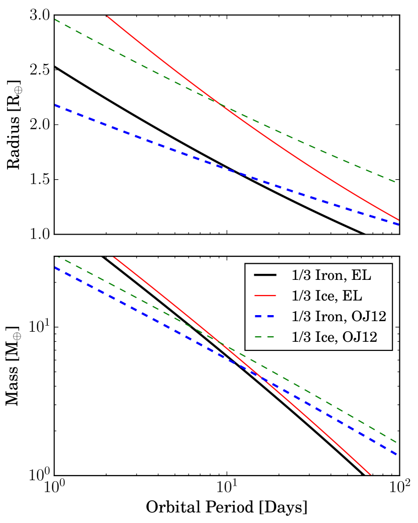
To further illustrate this effect, in Fig. 10, we plot the values of for Earth-like cores and those with a composition of 1/3 Ice, 2/3 silicates, using the Fortney et al. (2007) mass-radius relationship. This figure demonstrates that, with a large enough sample of planets, and a % radius errors, one could in principle distinguish between different evaporation models and different core compositions. The bottom panel translates the radius into planet core mass, demonstrating how the mass of the most massive stripped core depends on orbital period, for any of the models. Follow-up mass measurements can test these predictions.
Finally, we have not considered non-thermal escape processes such as stellar wind stripping. This is because hydrodynamic evaporation dominates for the separations we are interested in here (e.g. Murray-Clay et al., 2009). We have also not included the effects of a planetary magnetic field. Presence of a magnetic field strong enough to retain its dipolar structure (despite the evaporation) close to the planet may suppress the mass-loss rates significantly (e.g. Adams, 2011; Owen & Adams, 2014; Khodachenko et al., 2015; Owen & Adams, 2016). Unfortunately, it is unknown if the Kepler planets possess sufficiently strong fields.
4.6. Stellar Mass
The deficit of planets between and results from interaction between planet internal structure and photo-evaporation. It is not sensitive to stellar mass. Indeed Fulton et al. (2017) report that the valley remains the same for all stars in their sample.
On the other hand, the actual morphology of the valley, i.e., the relative height of the two peaks, the widths of the peaks, the shape of the valley in period space, etc., depends on stellar mass. When plotting planet radii for a population that have a spread in host masses, it is easiest to see the evaporation valley when the horizontal axis is chosen to be the period, not bolometric insolation as commonly assumed. As eq. (20) shows, if we assume that , the evaporation timescale scales with orbital period and stellar mass as,
| (32) |
i.e., a weak dependence on stellar mass. Alternatively, if one takes the horizontal axis as the stellar insolation (, or equivalently, planet equilibrium temperature),
| (33) |
This latter has a stronger mass dependence; as a result, the evaporation valley is less distinct (Fig. 10 of Fulton et al., 2017). Similarly, but to a lesser degree, is plotting by semi-major axis, with . Ultimately, the stellar mass independent variable to use is high energy exposure (the total received high-energy flux over the planet’s lifetime); however, the down side is high energy exposure is a model dependent quantity and not observationally accessible for individual planets. The current high energy flux received by a planet at billions of years evolution is not representative of its high energy exposure (e.g. Tu et al., 2015).
4.7. Two populations of planets?
Envelope stripping becomes decreasingly important as one moves away from the star. For our assumed population of gas-rich planets, this means, going outward, there should be fewer bare cores, and these bare cores should be lower in mass (smaller in size). For example, Fig. 5 (the dotted black line) indicates that there should be no bare planets of mass () beyond orbital periods of days and no bare planets of mass M⊕ beyond orbital periods of days (see also Lopez & Rice, 2016).888The variation of (§4.5) may extend this value out to days (Fig. 9) for bare 3 M⊕ planets and out to days for bare 1 M⊕ planets. Furthermore, Owen & Jackson (2012) showed that the hydrodynamical outflow we posit here do not happen for planets much outside days. Rather, the evaporative outflows is so rarefied the gas stops being collisional before the sonic point is reached and the mass-loss rate is instead determined by Jeans’ escape and falls much below the hydrodynamic value.
Interestingly, despite the selection effects against detecting small planets at large distances, they appear to be present in the Kepler sample.999The CKS sample does not contain enough detection in this range, and it is unclear what the stellar masses of individual planets are. The radius error bars remain large. And the abundance of such planets are not yet solidly established. However, if future observations confirm that such planets are abundant, this will require a separate population of planets than that posited here. This population is born bare.
5. Conclusions
We have developed a minimal analytical model which allows us to efficiently follow the evolution of low-mass planets, under the combined effects of cooling contraction and mass loss by evaporation, aside from illuminating the controlling physics. This model show that the mass-loss timescale peaks at around where planet sizes are doubled by their H/He envelopes, also where the envelope mass is of order a few percent. The timescale drops below this value because, while the envelope becomes more tenuous, the planet radii remain largely constant and so do the photo-evaporating fluxes they receive. The timescale also drops above this value because the planet swells up faster than the addition of envelope mass.
As a result, photoevaporation naturally gives rise to a final planet distribution that is bimodal in radius, peaking at the naked core size and twice its value. This then explains the observed radius “valley” in the California Kepler Survey sample (Fulton et al., 2017), as well as the steep fall-off of planets beyond in the general Kepler catalogue, for a single population of planets that are born with at least a few percent of H/He envelopes (“water-worlds” with water/steam envelopes are ruled out), this amount of gas lies above the most optimistic estimate for outgassing (Elkins-Tanton, 2008; Elkins-Tanton & Seager, 2008) and suggests that the envelopes were accreted from the protoplanetary discs. In the latter scenario, a few percent or more envelope mass may be natural (Rafikov, 2006). It is roughly the mass of an adiabatic envelope maintained by a planet of a few Earth masses at AU (but see Lee et al., 2014; Ginzburg et al., 2016, for modifications).
The positions of the peaks and valley also lead us to the following conclusions: the planet masses can be described by a Rayleigh distribution with a mode at , the cores have a composition that is ice-poor. Ice-rich cores move the gap too far above the observed value. The absence of icy cores indicates local assembly of the Kepler planets, as opposed to formation beyond the ice-line (followed by large-scale migration). Furthermore, as most of the erosion occurs before 100 Myrs, the Kepler planets must have reached their current orbital locations well before that time. This rules out the possibility that they were migrated in at late times by dynamical processes (e.g. high-eccentricity migration) and also rules out the suggestion that the dearth of intermediate sized planets on short orbits (the “sub-jovian pampas”) is entirely due to tidal stripping during dynamical migration (Matsakos & Königl, 2016). Lastly, current data allow the silicate-iron cores to have a wide spread in iron fraction.
Planets that can be stripped bare have vanishingly small mass at larger orbital periods. Our energy-limited model does not produce planets of size (or ) much beyond days. We investigate the impacts on this (and other) prediction by factors such as atmosphere metallicity, core luminosity, stellar mass, and evaporation efficiency. None made much difference except perhaps the last one. In our ad-hoc model where the efficiency is higher for less bound atmospheres, we are able to extend the above period limit to days. This gives hope that a large enough observational sample could discriminate various evaporation models.
Observationally, there is some evidence small planets appear to exist at orbital periods longer than days in the overall Kepler sample. They are possibly numerous given their low detection probability. If this is confirmed by future observations, then our one-population model, though appearing to explain many of the observed features inward of days, may be insufficient. There may need to be another population of low-mass planets that are born with essentially no envelopes. This separate population will need to have masses , so as not to fill in the evaporation valley. Orbital instabilities have been suggested to be common among Kepler systems (e.g., Pu & Wu, 2015). Giant impacts among short period planets will happen at speeds well above their surface escape velocities (Agnor & Asphaug, 2004; Marcus et al., 2009), and will therefore disperse much of the original planetary envelopes. Since these impacts will occur after the natal disk has dispersed, they may give rise to this new population.
Future improvements are needed to further solidify results here. Theoretically, our results are obtained using a minimal analytical model. This was a deliberate choice in order to provide a basic understanding for the origin of the evaporation valley. We have calibrated our model against mesa calculations, but it still contains a number of assumptions (e.g., constant evaporation efficiency). Work should be carried out with more accurate numerical planetary structure models and more physically motivated evaporation model to determine the exact nature of the birth properties of short-period, low-mass exoplanets. Observationally, planet properties will be refined further by future precision stellar data, allowing more detailed comparison. We have adopted a mass function for the Kepler planets that is Rayleigh with a mode of . This prediction should be tested by future mass measurements.
Notes in proof. While this paper was in review, Jin & Mordasini (2017) submitted a paper which used numerical modelling to reach much of the same conclusions about the composition of the Kepler planets as we do here. An interesting development comes from Dong et al. (2017) where they reported a population of “Hop-tunes”, Neptune-sized planets at close distances from their host stars, where we predict most planets should have been evaporated to bare cores. Intriguingly, this population only exists around metal-rich stars. This presents currently an unsolved puzzle.
References
- Adams et al. (2008) Adams, E. R., Seager, S., & Elkins-Tanton, L. 2008, ApJ, 673, 1160-1164
- Adams (2011) Adams, F. C. 2011, ApJ, 730, 27
- Agnor & Asphaug (2004) Agnor, C., & Asphaug, E. 2004, ApJ, 613, L157
- Baraffe et al. (2004) Baraffe, I., Selsis, F., Chabrier, G., et al. 2004, A&A, 419, L13
- Baraffe et al. (2006) Baraffe, I., Alibert, Y., Chabrier, G., & Benz, W. 2006, A&A, 450, 1221
- Batalha et al. (2013) Batalha, N. M., Rowe, J. F., Bryson, S. T., et al. 2013, ApJS, 204, 24
- Borucki et al. (2011) Borucki, W. J., Koch, D. G., Basri, G., et al. 2011, ApJ, 736, 19
- Burke et al. (2014) Burke, C. J., Bryson, S. T., Mullally, F., et al. 2014, ApJS, 210, 19
- Carter et al. (2012) Carter, J. A., Agol, E., Chaplin, W. J., et al. 2012, Science, 337, 556
- Charnay et al. (2015) Charnay, B., Meadows, V., & Leconte, J. 2015, ApJ, 813, 15
- Chen & Rogers (2016) Chen, H., & Rogers, L. A. 2016, ApJ, 831, 180
- Ciardi et al. (2013) Ciardi, D. R., Fabrycky, D. C., Ford, E. B., et al. 2013, ApJ, 763, 41
- Cox (2000) Cox, A. N. 2000, Allen’s Astrophysical Quantities,
- Davis & Wheatley (2009) Davis, T. A., & Wheatley, P. J. 2009, MNRAS, 396, 1012
- Dong et al. (2017) Dong, S., Xie, J.-W., Zhou, J.-L., Zheng, Z., & Luo, A. 2017, arXiv:1706.07807
- Dressing et al. (2015) Dressing, C. D., Charbonneau, D., Dumusque, X., et al. 2015, ApJ, 800, 135
- Ehrenreich et al. (2015) Ehrenreich, D., Bourrier, V., Wheatley, P. J., et al. 2015, Nature, 522, 459
- Elkins-Tanton (2008) Elkins-Tanton, L. T. 2008, Earth and Planetary Science Letters, 271, 181
- Elkins-Tanton & Seager (2008) Elkins-Tanton, L. T., & Seager, S. 2008, ApJ, 685, 1237-1246
- Erkaev et al. (2007) Erkaev, N. V., Kulikov, Y. N., Lammer, H., et al. 2007, A&A, 472, 329
- Erkaev et al. (2016) Erkaev, N. V., Lammer, H., Odert, P., et al. 2016, MNRAS, 460, 1300
- Fulton et al. (2017) Fulton, B. J., Petigura, E. A., Howard, A. W., et al. 2017, arXiv:1703.10375
- Fortney et al. (2007) Fortney, J. J., Marley, M. S., & Barnes, J. W. 2007, ApJ, 659, 1661
- Freedman et al. (2008) Freedman, R. S., Marley, M. S., & Lodders, K. 2008, ApJS, 174, 504-513
- Fressin et al. (2013) Fressin, F., Torres, G., Charbonneau, D., et al. 2013, ApJ, 766, 81
- Hadden & Lithwick (2014) Hadden, S., & Lithwick, Y. 2014, ApJ, 787, 80
- Hadden & Lithwick (2016) Hadden, S., & Lithwick, Y. 2016, arXiv:1611.03516
- Hernández et al. (2007) Hernández, J., Hartmann, L., Megeath, T., et al. 2007, ApJ, 662, 1067
- Howard et al. (2010) Howard, A. W., Marcy, G. W., Johnson, J. A., et al. 2010, Science, 330, 653
- Howard et al. (2012) Howard, A. W., Marcy, G. W., Bryson, S. T., et al. 2012, ApJS, 201, 15
- Howe & Burrows (2015) Howe, A. R., & Burrows, A. 2015, ApJ, 808, 150
- Ginzburg et al. (2016) Ginzburg, S., Schlichting, H. E., & Sari, R. 2016, ApJ, 825, 29
- Güdel et al. (1997) Güdel, M., Guinan, E. F., & Skinner, S. L. 1997, ApJ, 483, 947
- Jackson et al. (2012) Jackson, A. P., Davis, T. A., & Wheatley, P. J. 2012, MNRAS, 422, 2024
- Jin et al. (2014) Jin, S., Mordasini, C., Parmentier, V., et al. 2014, ApJ, 795, 65
- Jin & Mordasini (2017) Jin, S., & Mordasini, C. 2017, arXiv:1706.00251
- Johnson et al. (2017) Johnson, J. A., Petigura, E. A., Fulton, B. J., et al. 2017, arXiv:1703.10402
- Johnstone et al. (2015) Johnstone, C. P., Güdel, M., Stökl, A., et al. 2015, ApJ, 815, L12
- Jontof-Hutter et al. (2016) Jontof-Hutter, D., Ford, E. B., Rowe, J. F., et al. 2016, ApJ, 820, 39
- Kasting & Pollack (1983) Kasting, J. F., & Pollack, J. B. 1983, Icarus, 53, 479
- Khodachenko et al. (2015) Khodachenko, M. L., Shaikhislamov, I. F., Lammer, H., & Prokopov, P. A. 2015, ApJ, 813, 50
- Kulow et al. (2014) Kulow, J. R., France, K., Linsky, J., & Loyd, R. O. P. 2014, ApJ, 786, 132
- Lammer et al. (2003) Lammer, H., Selsis, F., Ribas, I., et al. 2003, ApJ, 598, L121
- Lecavelier Des Etangs (2007) Lecavelier Des Etangs, A. 2007, A&A, 461, 1185
- Lee et al. (2014) Lee, E. J., Chiang, E., & Ormel, C. W. 2014, ApJ, 797, 95
- Lee & Chiang (2015) Lee, E. J., & Chiang, E. 2015, ApJ, 811, 41
- Lopez et al. (2012) Lopez, E. D., Fortney, J. J., & Miller, N. 2012, ApJ, 761, 59
- Lopez & Fortney (2013) Lopez, E. D., & Fortney, J. J. 2013, ApJ, 776, 2
- Lopez & Fortney (2014) Lopez, E. D., & Fortney, J. J. 2014, ApJ, 792, 1
- Lopez (2016) Lopez, E. D. 2016, arXiv:1610.01170
- Lopez & Rice (2016) Lopez, E. D., & Rice, K. 2016, arXiv:1610.09390
- López-Morales et al. (2016) López-Morales, M., Haywood, R. D., Coughlin, J. L., et al. 2016, AJ, 152, 204
- Lundkvist et al. (2016) Lundkvist, M. S., Kjeldsen, H., Albrecht, S., et al. 2016, Nature Communications, 7, 11201
- Marcy et al. (2014) Marcy, G. W., Isaacson, H., Howard, A. W., et al. 2014, ApJS, 210, 20
- Marcus et al. (2009) Marcus, R. A., Stewart, S. T., Sasselov, D., & Hernquist, L. 2009, ApJ, 700, L118
- Mayor et al. (2011) Mayor, M., Marmier, M., Lovis, C., et al. 2011, arXiv:1109.2497
- Matsakos & Königl (2016) Matsakos, T., & Königl, A. 2016, ApJ, 820, L8
- Mulders et al. (2016) Mulders, G. D., Pascucci, I., Apai, D., Frasca, A., & Molenda-Żakowicz, J. 2016, AJ, 152, 187
- Murray-Clay et al. (2009) Murray-Clay, R. A., Chiang, E. I., & Murray, N. 2009, ApJ, 693, 23
- Morton et al. (2016) Morton, T. D., Bryson, S. T., Coughlin, J. L., et al. 2016, ApJ, 822, 86
- Owen & Jackson (2012) Owen, J. E., & Jackson, A. P. 2012, MNRAS, 425, 2931
- Owen & Wu (2013) Owen, J. E., & Wu, Y. 2013, ApJ, 775, 105
- Owen & Adams (2014) Owen, J. E., & Adams, F. C. 2014, MNRAS, 444, 3761
- Owen & Adams (2016) Owen, J. E., & Adams, F. C. 2016, MNRAS, 456, 3053
- Owen & Alvarez (2016) Owen, J. E., & Alvarez, M. A. 2016, ApJ, 816, 34
- Owen & Wu (2016) Owen, J. E., & Wu, Y. 2016, ApJ, 817, 107
- Owen & Morton (2016) Owen, J. E., & Morton, T. D. 2016, ApJ, 819, L10
- Paxton et al. (2011) Paxton, B., Bildsten, L., Dotter, A., et al. 2011, ApJS, 192, 3
- Paxton et al. (2013) Paxton, B., Cantiello, M., Arras, P., et al. 2013, ApJS, 208, 4
- Paxton et al. (2015) Paxton, B., Marchant, P., Schwab, J., et al. 2015, ApJS, 220, 15
- Petigura et al. (2013) Petigura, E. A., Marcy, G. W., & Howard, A. W. 2013, ApJ, 770, 69
- Petigura et al. (2017) Petigura, E. A., Howard, A. W., Marcy, G. W., et al. 2017, arXiv:1703.10400
- Pu & Wu (2015) Pu, B., & Wu, Y. 2015, ApJ, 807, 44
- Rafikov (2006) Rafikov, R. R. 2006, ApJ, 648, 666
- Ribas et al. (2005) Ribas, I., Guinan, E. F., Güdel, M., & Audard, M. 2005, ApJ, 622, 680
- Rogers & Seager (2010) Rogers, L. A., & Seager, S. 2010, ApJ, 712, 974
- Salz et al. (2016) Salz, M., Schneider, P. C., Czesla, S., & Schmitt, J. H. M. M. 2016, A&A, 585, L2
- Shematovich et al. (2014) Shematovich, V. I., Ionov, D. E., & Lammer, H. 2014, A&A, 571, A94
- Silburt et al. (2015) Silburt, A., Gaidos, E., & Wu, Y. 2015, ApJ, 799, 180
- Tian et al. (2005) Tian, F., Toon, O. B., Pavlov, A. A., & De Sterck, H. 2005, ApJ, 621, 1049
- Tu et al. (2015) Tu, L., Johnstone, C. P., Güdel, M., & Lammer, H. 2015, A&A, 577, L3
- Valencia et al. (2010) Valencia, D., Ikoma, M., Guillot, T., & Nettelmann, N. 2010, A&A, 516, A20
- West et al. (2008) West, A. A., Hawley, S. L., Bochanski, J. J., et al. 2008, AJ, 135, 785
- Wakeford et al. (2017) Wakeford, H. R., Sing, D. S., Kataria, T., et al. 2017 Science, 356, 628
- Weiss & Marcy (2014) Weiss, L. M., & Marcy, G. W. 2014, ApJ, 783, L6
- Wolfgang et al. (2016) Wolfgang, A., Rogers, L. A., & Ford, E. B. 2016, ApJ, 825, 19
- Wu & Lithwick (2013) Wu, Y., & Lithwick, Y. 2013, ApJ, 772, 74
- Yelle (2004) Yelle, R. V. 2004, Icarus, 170, 167
- Youdin (2011) Youdin, A. N. 2011, ApJ, 742, 38
- Zahnle & Catling (2017) Zahnle, K. J., Catling, D. C. 2017, arXiv:1702.03386
Appendix A The dimensionless integrals and
In § 2.1.1 we have introduced dimensionless integrals of the form:
| (A1) |
In the limit , or then is independent of and can be approximated as:
| (A2) |
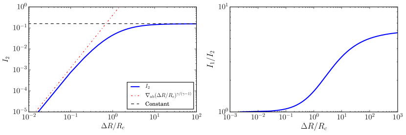
This result implies that the ratio for the case of a thin envelope. For the case of a puffy envelope, we need to consider how the varies with . For , the choice appropriate in our model, the integrand of eq. (A1) is, to first order, at small . Therefore, for the integral is not dominated close to and eq. (A1) becomes independent of as the envelope becomes large and becomes small. Thus in the limit of large atmospheres (), both and are constant and as such their ratio is also constant. In our model we require and the ratio explicitly. The full numerical solution of and the approximations discussed above are shown in the left-hand panel of Figure 11 and the full numerical solution of the ratio is shown in right-hand panel Figure 11.
