Thermodynamics of star polymer solutions: a coarse-grained study

Abstract

We consider a coarse-grained (CG) model with pairwise interactions, suitable to describe low-density solutions of star-branched polymers of functionality $f$. Each macromolecule is represented by a CG molecule with $(f+1)$ interaction sites, which captures the star topology. Potentials are obtained by requiring the CG model to reproduce a set of distribution functions computed in the microscopic model in the zero-density limit. Explicit results are given for $f=6,12$ and 40. We use the CG model to compute the osmotic equation of state of the solution for concentrations $c$ such that $\Phi_{p}=c/c^{*}\mathrel{\hbox to0.0pt{\lower 3.0pt\hbox{$\mathchar 536\relax$}\hss}\raise 2.0pt\hbox{$\mathchar 316\relax$}}1$, where $c^{*}$ is the overlap concentration. We also investigate in detail the phase diagram for $f=40$, identifying the boundaries of the solid intermediate phase. Finally, we investigate how the polymer size changes with $c$. For $\Phi_{p}\mathrel{\hbox to0.0pt{\lower 3.0pt\hbox{$\mathchar 536\relax$}\hss}\raise 2.0pt\hbox{$\mathchar 316\relax$}}0.3$ polymers become harder as $f$ increases at fixed reduced concentration $c/c^{*}$. On the other hand, for $\Phi_{p}\mathrel{\hbox to0.0pt{\lower 3.0pt\hbox{$\mathchar 536\relax$}\hss}\raise 2.0pt\hbox{$\mathchar 318\relax$}}0.3$, polymers show the opposite behavior: At fixed $\Phi_{p}$, the larger the value of $f$, the larger their size reduction is.

I Introduction

Soft materials are at present the object of very active research, because of their peculiar physico-chemical properties and for their technological applications. In particular, star polymers have attracted a considerable interest, GFHR-96 ; VFPR-01 as their thermodynamic and rheological behavior can be tuned by varying their functionalities (i.e., the number of their arms), thereby interpolating between the behavior observed using linear polymers and that appropriate for hard colloids.

Star-branched molecules of functionality $f$ are obtained by tethering $f$ polymer chains to a central core. Their structure in very dilute solutions in which one can neglect polymer-polymer interactions is very well understood, both at a qualitative and quantitative level, at least when the number $L$ of monomers per arm is large. For large $f$ and $L$, the behavior of star polymers is often modelled by using the Daoud-Cotton model. DC-82 ; BZ-84 The scaling predictions of this model are confirmed by numerical simulations, although they appear to be quantitatively valid only for $f\gg 100$. Grest-94 ; HNG-04 ; HG-04 ; HBL-09 ; RP-13 At finite density, the thermodynamic behavior of dilute and semidilute solutions of these macromolecules is well established from a qualitative point of view. Scaling arguments and approximate calculations predict a qualitative change of the phase diagram as $f$ increases. WP-86 ; WPC-86 ; LLWAKAR-98 ; WLL-98 ; WLL-99 ; LSLWRZ-05 ; MP-13 For $f$ less than a critical value $f_{c}$, star polymers behave as linear chains. As the density increases, polymers simply overlap, so that the behavior is qualitatively analogous to that of linear polymers. On the other hand, for $f>f_{c}$, a solid phase appears, separating two distinct (one dilute and one dense) fluid phases. At a quantitative level, however, much less is known in the universal, large-$L$ regime. Numerical simulations, which are at present the only method that provides accurate results, are quite hard. First, it is difficult to devise efficient algorithms for these finite-density systems and therefore simulations are very slow. Second, finite-length corrections increase quite rapidly with the functionality $f$ for fixed $L$.RP-13 Therefore, even when using optimal models, tuned to minimize this type of corrections, one still needs $L\mathrel{\hbox to0.0pt{\lower 3.0pt\hbox{$\mathchar 536\relax$}\hss}\raise 2.0pt\hbox{$\mathchar 318\relax$}}10^{2}$-$10^{3}$ to obtain results in the universal (model-independent) regime. Therefore, even for relatively small functionalities, say $f\approx 10$, one ends up with prohibitively large molecules.

Since we are only interested in thermodynamical and large-scale properties of the system, a numerically affordable method to overcome the above-mentioned difficulties consists in using coarse-grained (CG) models, in which most of the internal degrees of freedom of the polymer are treated implicitly, projecting the reference system onto a set of CG molecules with a limited number of interaction sites (we call them blobs). Several different CG strategies have been proposed in the literature: MP-02 ; Voth-09 ; Feller-09 ; Wilson-09 ; PK-09 ; RN-11 ; Noid-13 ; GSH-17 structure-based method, energy-based method, force-matching and relative-entropy approaches, just to mention the most popular ones. In this work we consider a CG model with effective pairwise interactions, which are obtained by using the structure-based route.LBHM-00 ; Likos-01 ; BLHM-01 ; MP-02 ; PCH-07 ; Pelissetto-09 ; PK-09 ; DPP-12-Soft ; DMPP-15-SpecTopics The potentials are obtained by requiring the CG model to reproduce a set of full-monomer (i.e., computed in the microscopic model) target distribution functions determined in the limit of zero density. As one needs to simulate only a small number of polymers to compute the target distributions, one can consider large molecules, thereby working in the large degree-of-polymerization, universal regime.

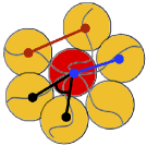
The simplest CG approach consists in replacing the whole polymer with a monoatomic molecule, obtaining the so-called single-blob (SB) model. The effective interactions for this simple representation have been either postulated by using phenomenological argumentsLLWAKAR-98 ; JDLvFL-01 or obtained by accurate numerical simulations.HG-04 These models provide the correct qualitative picture, LLWAKAR-98 ; WLL-98 ; WLL-99 ; MP-13 but are not meant to provide quantitatively accurate predictions unless the system is in the dilute regime, i.e., only for $\Phi_{p}\ll 1$, where $\Phi_{p}={4\over 3}\pi\rho_{p}\hat{R}_{g}^{3}$ ($\rho_{p}=N_{p}/V$, $N_{p}$ is the number of star polymers in a box of size $V$, and $\hat{R}_{g}$ is the average zero-density radius of gyration) is the polymer volume fraction. In this work we study the simplest generalization of the SB model that captures the star topology. Each star polymer is replaced by a CG molecule with $(f+1)$ blobs, see Fig. 1: one of them represents the center of the star, while the other $f$ blobs are associated with the arms. It is important to derive the limits of validity of this multiblob (MB) model. In Ref. PCH-07, it was shown that a multiblob model for linear polymers with $n$ effective sites is accurate up to $\Phi_{p}\mathrel{\hbox to0.0pt{\lower 3.0pt\hbox{$\mathchar 536\relax$}\hss}\raise 2.0pt\hbox{$\mathchar 316\relax$}}n^{3\nu-1}$ ($\nu\approx 0.588$ is the usual Flory exponent), a result that was confirmed by the simulations of Refs. DPP-12-Soft, ; DPP-12-JCP, . This argument should be applied with care to our star-polymer system. Although we take $(f+1)$ sites to describe each star polymer, due to its geometrical construction, the level of resolution of our model is not higher than that of a trimer representation, thus we should take $n=3$ in the general expression. Therefore, we expect accurate results only up to $\Phi_{p}\mathrel{\hbox to0.0pt{\lower 3.0pt\hbox{$\mathchar 536\relax$}\hss}\raise 2.0pt\hbox{$\mathchar 316\relax$}}3^{3\nu-1}\approx 2.4$. For this reason, we investigate the thermodynamic behavior up to $\Phi_{p}\approx 2$. This is not a serious limitation, as most of the interesting phenomena—for instance, the fluid-solid transition for large functionalities—occur for much lower densities, i.e., for $\Phi_{p}\mathrel{\hbox to0.0pt{\lower 3.0pt\hbox{$\mathchar 536\relax$}\hss}\raise 2.0pt\hbox{$\mathchar 316\relax$}}1.0$.

In this work we consider $f=6$, $f=12$, and $f=40$. For the two lowest values of $f$ the behavior should be qualitatively similar to that observed for linear chains, while for $f=40$ we expect a significantly different behavior, with the presence of ordering fluid-solid transitions.

The paper is organized as follows. In Sec. II we discuss the CG representation. In Sec. II.1 we give the definitions and present the general strategy, which follows closely what has been done for linear polymers in Ref. DPP-12-Soft, . Then, we present our results for the target distribution functions in Sec. II.2. In Sec. III we compute the effective interactions for the CG model. In Sec. B.5 we use the model to investigate the thermodynamic behavior. In Sec. V we focus on the location of the fluid-solid transitions (more details are reported in the supplementary material) and give preliminary results for the stable crystal structures. In Sec. VI we discuss how the polymer size changes at finite density. Finally, in Sec. VII we draw our conclusions. In the Appendix we give some details on the inversion precedure used to determine the intermolecular potentials.

II The coarse-grained representation

II.1 Definitions and general strategy

Figure 1: Schematic representation of a star polymer with $f$ arms: the polymer is divided into $(f+1)$ subunits (blobs), one for the center and one for each arm.

In this section we define the CG model, following the same strategy used for linear polymers in Ref. DPP-12-Soft, and recently reviewed in Ref. DMPP-15-SpecTopics, . The simplest model that captures the star topology is obtained by replacing the polymer with a CG molecule made of $(f+1)$ atoms (we call them blobs): one of them represents the center of the star, while the other $f$ blobs are associated with the arms, see Fig. 1.

To be specific we consider a star polymer with $f$ arms and $L$ monomers per arm. We label each arm with a Greek index $\alpha$, $\alpha=1,\ldots,f$, and the monomer positions with ${\bm{r}}_{\alpha,i}$, $i=1,\ldots,L-1$. The central monomer position is ${\bm{r}}_{0}$. To each star, we associate a CG representation $\{{\bm{R}}_{0},{\bm{R}}_{1},\ldots,{\bm{R}}_{f}\}$, where

$${\bm{R}}_{0} = {1\over mf}\left(f{\bm{r}}_{0}+\sum_{\alpha=1}^{f}\sum_{i=1}^{m-1}{\bm{r}}_{\alpha,i}\right),$$

$${\bm{R}}_{\alpha} = {1\over mf}\sum_{i=m}^{L-1}{\bm{r}}_{\alpha,i},$$ (1)

are the centers of mass of the central blob and of the blobs associated with the arms, respectively, and $m=L/(f+1)$ [$L$ is assumed to be a multiple of $(f+1)$]. Note that, for convenience, we have given a weight $f$ to the core monomer. As discussed in Ref. HNG-04, , this is irrelevant in the large-$L$ limit. For this representation, we define a set of intramolecular and intermolecular distribution functions that are used as targets for the CG model. First, we consider the adimensional intramolecular distribution functions

$$P_{\alpha\beta}(b) = \hat{R}_{g}\langle\delta(|{\bm{R}}_{\alpha}-{\bm{R}}_{\beta}|-r)\rangle,$$ (2)

where $\hat{R}_{g}$ is the zero-density radius of gyration (here and in the following we will use a hat to indicate that a given quantity is computed at zero density) and the average is over all conformations of a single isolated star. In the large-$L$ limit these quantities are functions of the ratio $b=r/\hat{R}_{g}$ and are universal, in the sense that they do not depend on the microscopic polymer model. We also consider the distribution of the angle between two arms ($1\leq\alpha,\beta\leq f$)

$$P_{\rm th,\alpha\beta}(\cos\theta)=\left\langle\delta\left({({\bm{R}}_{\alpha}-{\bm{R}}_{0})\cdot({\bm{R}}_{\beta}-{\bm{R}}_{0})\over|{\bm{R}}_{\alpha}-{\bm{R}}_{0}||{\bm{R}}_{\beta}-{\bm{R}}_{0}|}-\cos\theta\right)\right\rangle.$$ (3)

Finally, we consider the intermolecular blob-blob potentials of mean force

$$\beta W_{\alpha\beta}(b)=-\ln\langle e^{-\beta U_{\rm inter}}\rangle_{{\bm{R}}_{\alpha}^{(1)}=0,R_{\beta}^{(2)}=r}\,,$$ (4)

where $U_{\rm inter}$ is the intermolecular potential energy, and the average is over all configurations of pairs of noninteracting star polymers such that blob $\alpha$ of the first polymer is in the origin (${\bm{R}}_{\alpha}^{(1)}=0$), and blob $\beta$ of the second polymer is located in any point at a distance $r$ from the origin.

In the CG model the basic object is a polyatomic molecule with $(f+1)$ atoms located in ${\bf R}_{0},\ldots,{\bf R}_{f}$. All length scales are expressed in terms of $\hat{R}_{g}$, hence potentials and distribution functions depend on the adimensional combination ${\bm{b}}={\bm{R}}/\hat{R}_{g}$. In an exact CG procedure the intramolecular potential is a function of the coordinates of all atoms. As in our previous work on linear polymers,DPP-12-Soft we perform a drastic simplification. We only consider potentials that depend on a single scalar variable and, moreover, we neglect all interactions that involve more than three blobs. In spite of these simplifications, we expect this parametrization of the intramolecular interactions to provide reasonably accurate results. In the case of linear polymers, we observed the appearance of a well-defined hierarchy among the $n$-body interactions: $V_{\rm 2-body}\gg V_{\rm 3-body}\gg V_{\rm 4-body}\ldots$ We expect (and we will provide evidence below) the same here, so that the neglect of all $n$-body interactions with $n\geq 4$ should have a limited impact on the accuracy of the model. Guided by the parametrization of the intramolecular interactions used for linear polymers,DPP-12-Soft we write the intramolecular potential energy as, see Fig. 2,

$$U^{\rm intra} = \sum_{1\leq\alpha<\beta\leq f}V_{aa}(b_{\alpha\beta})+\sum_{1\leq\alpha\leq f}V_{ca}(b_{0\alpha})$$ (5)

$$+\sum_{1\leq\alpha<\beta\leq f}V_{\rm th}(\cos\theta_{\alpha\beta}),$$

where $b_{\alpha\beta}=|{\bm{R}}_{\alpha}-{\bm{R}}_{\beta}|/\hat{R}_{g}$, and $\theta_{\alpha\beta}$ is the angle between ${\bm{R}}_{\alpha}-{\bm{R}}_{0}$ and ${\bm{R}}_{\beta}-{\bm{R}}_{0}$. The three independent (arm-arm, center-arm, and angular) intramolecular potentials are determined by requiring the adimensional distributions $P_{\alpha\beta}$ and $P_{\rm th,\alpha\beta}$ to be identical in the polymer microscopic model and in the CG model.

Figure 2: Top: Intramolecular interactions; we consider potentials depending on the center-arm (blue line) and arm-arm distance (red line), and on the arm-arm angle (black line). Bottom: Intermolecular interactions: we consider pair potentials depending on the center-arm (blue line), arm-arm (red line), and center-center (black line) distance.

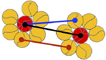
In the case of the intermolecular interactions, we only consider blob-blob pair potentials. Again this choice is motivated by feasibility and justified by our previous work on linear polymers and polymer-colloid mixtures.DMPP-15-SpecTopics In all cases, this simple parametrization provided accurate results. For the CG model of star polymers, we must introduce three different pair interactions, as we must distinguish the central blob from those associated with the arms. Therefore, the intermolecular potential energy for two CG star polymers is written as, see Fig. 2:

$$U^{\rm inter} = \sum_{\alpha,\beta=1}^{f}{\widetilde{V}}_{aa}(b_{\alpha\beta})+$$ (6)

$$\sum_{\alpha=1}^{f}[{\widetilde{V}}_{ca}(b_{0\alpha})+{\widetilde{V}}_{ca}(b_{\alpha 0})]+{\widetilde{V}}_{cc}(b_{00}),$$

where $b_{\alpha\beta}=|{\bm{R}}_{\alpha}^{(1)}-{\bm{R}}_{\beta}^{(2)}|/\hat{R}_{g}$, and $\{{\bm{R}}_{\alpha}^{(1)}\}$, $\{{\bm{R}}_{\alpha}^{(2)}\}$ are the coordinates of the blobs belonging to the two polymers. The three independent (arm-arm, center-arm, and center-center) potentials are determined so as to reproduce the potentials of mean force (4) in the full-monomer model.

II.2 Determination of the full-monomer distributions

Figure 3: Intramolecular distribution functions for $f=6$ and 40. Top: arm-arm (a-a) and center-arm (c-a) distance distributions as a function of $b=r/\hat{R}_{g}$. Bottom: angle distributions as a function of $\cos\theta$.

To compute the distributions (2) and (3), and the potentials of mean force (4), we perform Monte Carlo simulations of the lattice Domb-Joyce model DJ-72 at a particular value of the repulsion parameter that guarantees the absence of the leading large-$L$ correctionsCMP-06 ; DPP-16 (see the supplementary material for details). Such a model, that we already used in Ref. RP-13, , is particularly convenient, as it allows us to simulate very large systems and to obtain asymptotic large-$L$ results with good accuracy. Although in this paper we focus on $f=6,12$, and 40, we also determine the intramolecular distributions and the potentials of mean force for $f=18,24$, and $30$. We perform simulations for several values of $L$, in the range $100\mathrel{\hbox to0.0pt{\lower 3.0pt\hbox{$\mathchar 536\relax$}\hss}\raise 2.0pt\hbox{$\mathchar 316\relax$}}L\mathrel{\hbox to0.0pt{\lower 3.0pt\hbox{$\mathchar 536\relax$}\hss}\raise 2.0pt\hbox{$\mathchar 316\relax$}}1000$, without observing a significant $L$ dependence within the statistical accuracy. This is clearly due to the optimality of the model that minimizes the $L$-dependent corrections.footnote:optimality The results we use in the CG procedure are those corresponding to star polymers with $L\approx 1000$.

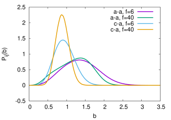
In Fig. 3 we report the center-arm distribution $P_{ca}(b)$, defined as the average of $P_{0\alpha}(b)$ over all arms ($\alpha\geq 1$), and the arm-arm distribution $P_{aa}(b)$, which is the average of $P_{\alpha\beta}(b)$ over all arm pairs ($\alpha,\beta\geq 1$). The distribution $P_{ca}(b)$ becomes more peaked as $f$ increases, indicating that the radial fluctuations of the arm centers of mass are suppressed for $f\to\infty$. Instead, the position of the maximum changes only slightly. If we compute the average squared distance $R^{2}_{ca}$ between the center of mass of the central blob (for large $f$ it coincides with the center of the star) and that of a polymer arm, we obtain $R_{ca}/\hat{R}_{g}=0.98,0.93,0.91,0.90$ for $f=6,12,30$, 40, respectively. We can compare these results with the predictions of the Daoud-Cotton model. DC-82 Let us assume that each arm is confined in a cone of solid angle $4\pi/f$ with the vertex in the center of the star and that the arm monomers are distributed with density $\rho(r)$, that only depends on the distance $r$. For large $f$ we can neglect the central blob, so that

$$R^{2}_{ca}={1\over L}\int r^{2}dr\int_{0}^{\theta_{0}}\sin\theta d\theta\int_{0}^{2\pi}d\phi\rho(r)(r\cos\theta)^{2},$$ (7)

with $1-\cos\theta_{0}=2/f$. For large $f$, this expression becomes

$$R^{2}_{ca}={4\pi\over Lf}\int drr^{4}\rho(r)={1\over Lf}\int d^{3}r\,r^{2}\rho(r)=\hat{R}_{g}^{2}.$$ (8)

This simple argument predicts $R_{ca}/\hat{R}_{g}=1$, which slightly overestimates the correct result. Clearly, arms are not confined in a single cone for large $f$, but are significantly intertwined, especially close to the center of the star. As a result, the arm center of mass is closer to the center than the Daoud-Cotton picture predicts.

The distribution $P_{aa}(b)$ is not very sensitive to $f$. It moves slightly towards smaller values of $b$ as $f$ increases, probably as a consequence of the fact that the arm centers of mass are closer to the star center. If we compute the average arm-arm square distance $R_{aa}^{2}$, we obtain $R_{aa}/\hat{R}_{g}=1.45,1,35,1.30,1.29$ for $f=6,12,30,40$. This is consistent with $R_{aa}=\sqrt{2}R_{ca}$, which is obtained by assuming that the arm centers of mass are randomly distributed on a sphere of radius $R_{ca}$.

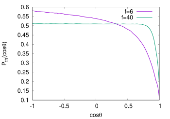
In Fig. 3 we also report the angle distribution $P_{\rm th}(\cos\theta)$. For $f=40$ it is approximately equal to 1/2 except for $\theta\mathrel{\hbox to0.0pt{\lower 3.0pt\hbox{$\mathchar 536\relax$}\hss}\raise 2.0pt\hbox{$\mathchar 316\relax$}}15^{\circ}$, which confirms that the arm centers of mass are distributed randomly around the center for large $f$. For $\theta\approx 0$ the distribution shows a dip. Note, however, that $P_{\rm th}(\cos\theta=1)$ increases as $f$ increases: we have $P_{\rm th}(1)\approx 0.1$, 0.15 for $f=6,40$, respectively. This suggests that, for large values of $f$, also the dip for $\theta\approx 0$ disappears and therefore the distribution becomes flat, implying the absence of correlations among the angular positions of the blobs. This result indicates that our parametrization of the intramolecular interactions should become increasingly accurate as $f$ increases: the neglected $n$-body correlations become irrelevant for stars of high functionality.

Figure 4: Potentials of mean force $\beta W_{{aa}}$ (arm-arm), $\beta W_{{ca}}$ (center-arm), and $\beta W_{{cc}}$ (center-center) as a function of $b=r/\hat{R}_{g}$, for star polymers with $f=6$ and 12 (top), and with $f=40$ (bottom, label FM). For $f=40$ we also report the potentials of mean force computed in the multiblob (MB) model, see Sec. III.2. They are essentially indistinguishable from the corresponding full-monomer quantities, confirming the accuracy of the inversion procedure.

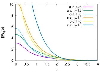
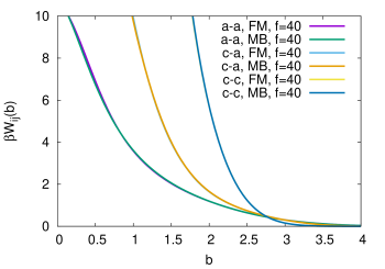
The potentials of mean force (again we average over all equivalent arms) are reported in Fig. 4. They depend on $f$ and show that stars become significantly less penetrable as $f$ increases. For instance, for $f=6$ and 12 we have $\beta W_{aa}(b=0)=3.1,4.7$, while $\beta W_{aa}(b)\mathrel{\hbox to0.0pt{\lower 3.0pt\hbox{$\mathchar 536\relax$}\hss}\raise 2.0pt\hbox{$\mathchar 318\relax$}}10$ for $f=40$. As expected, for large values of $f$, blobs of two different stars cannot fully overlap: blobs are densely packed, and therefore, when a blob of one polymer moves closer to a blob of a second polymer, it feels the strong repulsion of the close neighboring blobs, which forbids a significant overlap. This is also confirmed by the fact that, for large $f$, $\beta W_{aa}(b)$ decays slowly with $b$. For $f=40$, if $\hat{r}_{g}$ is the average radius of gyration of the blob ($\hat{r}_{g}\approx 0.45\hat{R}_{g}$), we have $\beta W_{aa}(2\hat{r}_{g}/\hat{R}_{g})\approx 4.0$: blobs of different polymers rarely overlap. This is good news for our CG procedure, which is reliable only if there is little overlap among blobs of different chains. The range of the potentials of mean force is approximately $3\hat{R}_{g}$, in agreement with the analysis of the monomer distribution of Ref. RP-13, . However, note the presence of a longer tail in $W_{aa}(b)$ which decreases slowly with $b$. Such tail has a simple geometrical interpretation. Since the center-arm distance is of order of $R_{ca}$, we expect contributions to $W_{aa}(b)$ at least up to $4R_{ca}\approx 4\hat{R}_{g}$ (two arms at the opposite sites of the two interacting stars).

III Determination of the coarse-grained potentials

III.1 Intramolecular potentials

Figure 5: Intramolecular potentials for $f=6$, 12 and 40. Top: center-arm potential $\beta V_{ca}(b)$; middle: arm-arm potential $\beta V_{aa}(b)$; bottom: angular potential $\beta V_{th}(\cos\theta)$. All potentials are normalized so that their minimum value is zero.

The CG multiblob potentials $\beta V_{ca}(b)$, $\beta V_{aa}(b)$, and $\beta V_{\rm th}(\cos\theta)$ are determined by enforcing the equality of the intramolecular distribution functions

$$P^{FM}_{i}(x_{i})=P^{CG}_{i}(x_{i}),$$ (9)

where the superscripts FM and CG refer to the full-monomer atomistic model and to the coarse-grained model, respectively, and the distributions $P_{i}$, $i=1,2,3$, correspond to the three functions $P_{aa}$, $P_{ca}$, and $P_{\rm th}$ defined in the previous Section. For this purpose, we use the iterative Boltzmann inversion (IBI) method.Schommers-83 ; MP-02 ; RPMP-03 We set $\beta V_{(0,i)}^{CG}(x_{i})=-\ln P^{FM}_{i}(x_{i})$ and then we use an iterative procedure that generates a sequence of approximations $\beta V_{(n,i)}^{CG}(x_{i})$, $n=1,2,\ldots$,

$$\beta V_{(n+1,i)}^{CG}(x_{i})=\beta V_{(n,i)}^{CG}(x_{i})-a\ln{\left(\frac{P_{i}^{FM}(x_{i})}{P_{(n,i)}^{CG}(x_{i})}\right)},$$ (10)

where $P_{(n,i)}^{CG}(x_{i})$ is the distribution function computed in the CG model with potentials $V_{(n,i)}^{CG}(x_{i})$. Here $a$ is a mixing parameter, which is tuned to optimize the convergence of the iterations. For $f=40$, we start with $a=0.2$ and decrease it systematically till $a=0.1$. Convergence is achieved after 100 iterations.

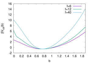
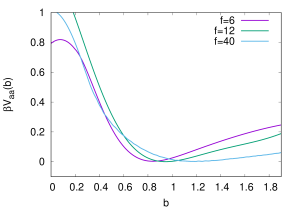
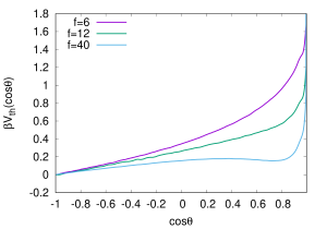
The potentials are reported in Fig. 5 for $f=6$, 12, and 40. They are normalized so that their minimal value is zero. We are not able to determine them accurately for small $b$ ($b\mathrel{\hbox to0.0pt{\lower 3.0pt\hbox{$\mathchar 536\relax$}\hss}\raise 2.0pt\hbox{$\mathchar 316\relax$}}0.2$, say), as the corresponding distribution functions are very small, and therefore not accurate, in this region. However, for the same reason, the probability that two blobs are so close is tiny. Hence, this lack of accuracy is not relevant in practice. The center-arm potential $V_{ca}(b)$ is repulsive at short distances where blobs overlap, takes its minimum for $b\approx 0.8$, and has a strong attractive tail at large distances, which is necessary to bind each arm to the center of the star. It is soft for $f=6$, with $V_{ca}(b=0)\approx 2.8k_{B}T$ at full overlap, but it becomes harder and narrower for $f=40$. For this value of $f$, we have $V_{ca}(b=0)\mathrel{\hbox to0.0pt{\lower 3.0pt\hbox{$\mathchar 536\relax$}\hss}\raise 2.0pt\hbox{$\mathchar 318\relax$}}10k_{B}T$, confirming the increasing conformational rigidity of the star polymer as $f$ increases. The arm-arm potential $V_{aa}(b)$ has a soft, repulsive core, which increases slightly with $f$, and an attractive tail, whose strength decreases as $f$ increases. The angular potential $V_{\rm th}(\cos\theta)$ is repulsive and takes its maximum for $\theta=0$, as a consequence of the repulsive interaction among different arms. As $f$ increases, $V_{\rm th}(\cos\theta=1)$ decreases and we expect the potential to vanish everywhere for large values of $f$.

$f$	FM	CG
6	0.759	0.760
12	0.772	0.771
40	0.793	0.795

Table 1: Ratio $\hat{R}^{2}_{g,b}/\hat{R}^{2}_{g}$ for $f=6$, 12, and 40, computed in the full-monomer (FM) and (CG) models, for an isolated star polymer (zero-density limit). Here $\hat{R}_{g,b}$ is the zero-density blob radius of gyration, see Eq. (11) for the definition.

In order to assess the accuracy of the inversion procedure, we consider the average radius of gyration $R_{g,b}$ of the CG molecule, which should coincide with

$$R^{2}_{g,b}=\frac{1}{2(f+1)^{2}}\left\langle\sum_{i,j=0}^{f}({\bm{R}}_{i}-{\bm{R}}_{j})^{2}\right\rangle$$ (11)

in the CG representation of the polymer. Note that it does not coincide with the radius of gyration ${R}_{g}$ of the original molecule. The two quantities satisfy the exact relationDPP-12-Soft

$${R}^{2}_{g}={R}^{2}_{g,b}+{r}^{2}_{g,b},$$ (12)

which also holds for each polymer chain. Here ${r}^{2}_{g,b}$ is the average blob radius of gyration

$${r}^{2}_{g,b} =\frac{1}{(f+1)}\sum_{\alpha=0}^{f}{r}^{2}_{g,b,\alpha},$$

$${r}^{2}_{g,b,\alpha} =\frac{1}{2mf}\left<\sum_{j,k=1}^{mf}({\bm{r}}_{j}^{\alpha}-{\bm{r}}_{k}^{\alpha})^{2}\right>,$$ (13)

where ${\bm{r}}_{k}^{\alpha}$ are the positions of the monomers belonging to blob $\alpha$ and $m=L/(f+1)$. In Table 1, we report the ratio $\hat{R}^{2}_{g,b}/\hat{R}^{2}_{g}$ for an isolated polymer (we remind the reader that a hat indicates that the corresponding quantity has been determined in the zero-density limit), comparing full-monomer and multiblob results. Differences are small, confirming the accuracy of the inversion procedure. From the data reported in Table 1, we can also estimate the average radius of gyration of the blobs in the zero-density limit. Using Eq. (12), we obtain $\hat{r}_{g}/\hat{R}_{g}=0.49,0.48,0.45$ for $f=6,12,40$. Note that, in spite of the fact that the star polymer is significantly more packed and dense as $f$ increases, $\hat{r}_{g}$ changes only slightly with the number of arms, another indication that different blobs strongly overlap.

III.2 Intermolecular interactions

We now compute the three intermolecular potentials, $\beta\widetilde{V}_{ca}(b)$, $\beta\widetilde{V}_{aa}(b)$, and $\beta\widetilde{V}_{cc}(b)$, requiring the CG model to reproduce the full-monomer mean-force potentials, i.e., enforcing

$$\beta W^{CG}_{ij}(b)=\beta W^{FM}_{ij}(b),$$ (14)

where $ij=cc$, $aa$, and $ca$. The determination of the potentials satisfying this condition is not trivial, and we have used a different strategy for the low-functionality stars ($f=6$ and $12$) and for $f=40$. In the first case we have essentially used the IBI method, Schommers-83 ; MP-02 ; RPMP-03 while for large functionalities a different procedure has to be employed. Details are given in the Appendix.

In all cases we obtain relatively short-range potentials, which are able to reproduce well the long tails that are present in the potentials of mean force. This is very relevant for the thermodynamic consistency of the CG approach, as tails give an important contribution to the pressure. Therefore, matching the tails is essential to obtain the correct thermodynamics.

The results for $f=6$ and 12 are shown in Fig. 6. It is important to stress that we are able to compute each potential only for those values of $b$ for which $W^{FM}_{ij}(b)$ is not too large (in practice we only consider the regions in which $\beta W^{FM}_{ij}(b)\mathrel{\hbox to0.0pt{\lower 3.0pt\hbox{$\mathchar 536\relax$}\hss}\raise 2.0pt\hbox{$\mathchar 316\relax$}}10$). In particular, the center-center potential is determined only for $b\mathrel{\hbox to0.0pt{\lower 3.0pt\hbox{$\mathchar 536\relax$}\hss}\raise 2.0pt\hbox{$\mathchar 318\relax$}}0.2$, 0.8 for $f=6$, 12, respectively. This is not a limitation, however, since the probability that the centers of the two stars are so close is always extremely low, see Fig. 4.

Figure 6: Intermolecular potentials for $f=6$ and 12. We report the arm-arm potential $\beta\widetilde{V}_{aa}$, the center-arm potential $\beta\widetilde{V}_{ca}$, and the center-center potential $\beta\widetilde{V}_{cc}$. The latter is only meaningful for $b\mathrel{\hbox to0.0pt{\lower 3.0pt\hbox{$\mathchar 536\relax$}\hss}\raise 2.0pt\hbox{$\mathchar 318\relax$}}0.2$ and 0.8 for $f=6$ and 12, respectively.

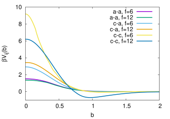
For both values of $f$, the arm-arm interaction is purely repulsive and soft at contact: $\widetilde{V}_{aa}(b=0)\approx 1.5k_{B}T$. It increases only slightly from $f=6$ to $f=12$. The center-arm interaction is more repulsive than the arm-arm interaction, $\widetilde{V}_{ca}(b=0)\approx 3k_{B}T$, $3.5k_{B}T$ for $f=6$ and 12, respectively, but the two potentials have approximately the same range. The center-center potential is the most repulsive interaction. Note that the potentials we have determined show the unexpected feature that $\widetilde{V}_{cc}(b)$ decreases for small values of $b$ as $f$ increases. This behavior, however, occurs in the region in which the $f=12$ potential cannot be trusted, and it is most likely incorrect. More interestingly, the center-center potential has an attractive tail for $r/\hat{R}_{g}\mathrel{\hbox to0.0pt{\lower 3.0pt\hbox{$\mathchar 536\relax$}\hss}\raise 2.0pt\hbox{$\mathchar 318\relax$}}1$, whose depth increases slightly from $f=6$ to $f=12$.

Figure 7: Intermolecular potentials of the multiblob model for $f=40$. We show the arm-arm potential $\beta\widetilde{V}_{aa}$, the center-arm potential $\beta\widetilde{V}_{ca}$ (valid for $b\mathrel{\hbox to0.0pt{\lower 3.0pt\hbox{$\mathchar 536\relax$}\hss}\raise 2.0pt\hbox{$\mathchar 318\relax$}}1.0$), and the center-center potential $\beta\widetilde{V}_{cc}$ (valid for $b\mathrel{\hbox to0.0pt{\lower 3.0pt\hbox{$\mathchar 536\relax$}\hss}\raise 2.0pt\hbox{$\mathchar 318\relax$}}1.9$).

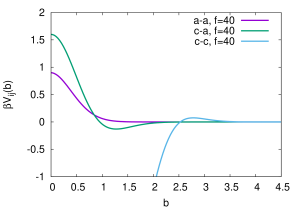The potentials $\widetilde{V}_{ij}(b)$ for $f=40$ are reported in Fig. 7. They are only relevant where $\beta W_{ij}(b)\mathrel{\hbox to0.0pt{\lower 3.0pt\hbox{$\mathchar 536\relax$}\hss}\raise 2.0pt\hbox{$\mathchar 316\relax$}}10$. Therefore, the center-arm and the center-center potentials cannot be trusted for distances $b\mathrel{\hbox to0.0pt{\lower 3.0pt\hbox{$\mathchar 536\relax$}\hss}\raise 2.0pt\hbox{$\mathchar 316\relax$}}1$ and $b\mathrel{\hbox to0.0pt{\lower 3.0pt\hbox{$\mathchar 536\relax$}\hss}\raise 2.0pt\hbox{$\mathchar 316\relax$}}1.9$, respectively. The potentials reproduce quite accurately the target distributions. A detailed analysis of the errors, see Appendix, indicates that $\widetilde{V}_{aa}(b)$ and $\widetilde{V}_{ca}(b)$ have an accuracy of 1%. The center-center potential is less accurate, with an error of at most 5%.

The arm-arm potential is soft, $\beta\widetilde{V}_{aa}(b=0)\approx 0.9$, and decreases rapidly. For $b=1$ we have $\beta\widetilde{V}_{aa}(b)\approx 0.062$, which is very close to the value it assumes for $f=6$ and 12. This is consistent with the idea that the range of the potential is of the order of $2\hat{r}_{g}\approx\hat{R}_{g}$. The center-arm potential is small and attractive in the relevant region $b\mathrel{\hbox to0.0pt{\lower 3.0pt\hbox{$\mathchar 536\relax$}\hss}\raise 2.0pt\hbox{$\mathchar 318\relax$}}1$. For $b=1$, $\beta\widetilde{V}_{ca}\approx-0.04$, while at the minimum (located at $b\approx 1.28$) we have $\beta\widetilde{V}_{ca}\approx-0.13$. Finally, the center-center potential is attractive for $b\mathrel{\hbox to0.0pt{\lower 3.0pt\hbox{$\mathchar 536\relax$}\hss}\raise 2.0pt\hbox{$\mathchar 316\relax$}}2.5$—this also occurs for $f=6$ and 12—and then it has a small repulsive tail.

IV Thermodynamic behavior

In this section, we analyze the thermodynamic and structural properties of star polymer solutions under good-solvent conditions, both at zero and finite density. The results we obtain using the CG multiblob (MB) model will then be compared with those obtained using the SB model, in which stars are represented by monoatomic molecules interacting by means of pair potentials. We use two different SB representations. First, we consider the midpoint (MP) representation, in which we take the center of the star as interaction site (this is the one mostly considered in SB studies, see, e.g., Refs. LLWAKAR-98, ; Likos-01, ). For linear polymers (they can be viewed as stars with $f=2$ arms), it corresponds to taking the central monomer as interaction site. A second possibility consists in taking the polymer center of mass (CM) as interaction site. For linear polymers (therefore, for $f=2$), the CM representation is more accurate than the MP one. DMPP-15-SpecTopics As $f$ increases, the CM of the star converges to the polymer center and therefore the two representations become equivalent for large $f$. Therefore, we present results for the two different choices only for $f=6$ and $f=12$. For $f=40$ there is little difference between them. For the MP case, we use the pair potentials reported in Ref. HG-04, . For the CM representation we have determined the potentials numerically using the optimal Domb-Joyce lattice model.DJ-72

IV.1 Zero density

	$f=6$		$f=12$		$f=40$
	$A_{2}$	$A_{3}$	$A_{2}$	$A_{3}$	$A_{2}$	$A_{3}$
SB-CM	14.15	88.43	23.70	288.96	42.39	1040
SB-MP	14.66	85.6	23.97	288
MB	14.231(4)	88.6(6)	23.78(5)	289(2)	41.91(2)	1028(6)
FM	14.202(12)	90.3(4)	23.54(3)	290(2)	41.90(11)	1031(13)

Table 2: Universal adimensional combinations $A_{2}$ and $A_{3}$ for $f=6$, 12. We give results obtained by using single-blob models, in the center-of-mass (SB-CM) and center (SB-MP) representations, and the multiblob model (MB). We also report the full-monomer (FM) results of Ref. RP-13, .

At zero density the accuracy of the CG model can be tested by comparing CG and full-monomer estimates of the universal adimensional coefficients $A_{n}=B_{n}/\hat{R}^{3(n-1)}_{g}$, where $B_{n}$ is the $n$-th virial coefficient. As discussed in Ref. DPP-12-Soft, , the comparison of $A_{2}$ provides a test of the inversion procedure. Results (virial coefficients are computed as discussed in Refs. CMP-06, ; CMP-08-virial, ) are reported in Table 2. The results obtained by using the SB model in the CM representation and the MB model are very close to the FM ones of Ref. RP-13, . Differences are less than 1%. Slightly larger differences (approximately 3%) are obtained in the MP representation. They are due to the slight inaccuracy of the interpolating formula of Ref. HG-04, .

Let us now compare the third virial combination $A_{3}$, which gives information on the relevance of the three-body interactions.DMPP-15-SpecTopics As it can be seen from Table 2, all CG results are close to the FM ones. Clearly, at least in the small-density region, the thermodynamics is controlled by pair interactions, at variance with what happens with linear polymers (in that case $A_{3}$ is understimated by 21% in the CM representation and by 50% in the MP representation DMPP-15-SpecTopics ). This is probably due to the fact that stars are more compact objects, so multiple overlaps are rare. These results confirm the assumption that the description in terms of pair interactions becomes more accurate as $f$ increases in the very dilute regime.

IV.2 Finite-density results: $f=6$ and $f=12$

Figure 8: Expected phase diagram for star polymers. Here $f$ is the functionality of the polymer and $\Phi_{p}$ the polymer volume fraction. “S” corresponds to a solid intermediate phase, “F” to a fluid phase.

Figure 9: Osmotic coefficient $Z=\beta P/\rho_{p}$ as a function of the volume fraction $\Phi_{p}$, for $f=6$ (top) and $f=12$ (bottom). We report multiblob (MB) estimates, single-blob results in the center of mass (SB-CM) and center (SB-MP) representations, and the extrapolation (16) (PADE).

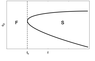
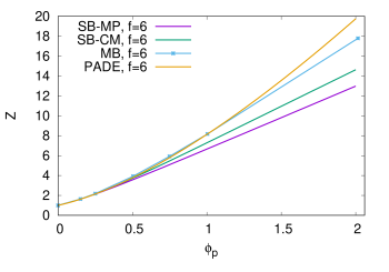
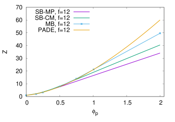
At finite density, star polymers are supposed to have two distinct behaviors depending on the functionality $f$. For small values of $f$, the density can be increased at will and polymers smoothly go from the dilute regime to the semidilute one, and finally, to the melt. On the other hand, for large $f$, a fluid-solid transition occurs in the dilute regime, with the appearance of a solid intermediate phase. WPC-86 ; WP-86 ; WLL-98 The transition is expected to occur for $f>f_{c}$, see Fig. 8, where $f_{c}$ is predicted by SB models to be in the rangeWLL-98 ; MP-13 $30\mathrel{\hbox to0.0pt{\lower 3.0pt\hbox{$\mathchar 536\relax$}\hss}\raise 2.0pt\hbox{$\mathchar 316\relax$}}f_{c}\mathrel{\hbox to0.0pt{\lower 3.0pt\hbox{$\mathchar 536\relax$}\hss}\raise 2.0pt\hbox{$\mathchar 316\relax$}}40$. For this reason, we consider here only the results for $f=6$ and 12. Results for $f=40$ are discussed in the next section.

We determined the osmotic coefficient

$$Z={\beta P\over\rho_{p}},$$ (15)

which is a universal function of $\Phi_{p}$ in the large-$L$ limit. For SB models, $Z$ was computed by using integral equation methods hansen:liquids and the Rogers-Young closure.RY-84 For a few selected values of $\Phi_{p}$, we also computed $Z$ by Monte Carlo simulations, obtaining results in perfect agreement with the Rogers-Young estimates, see supplementary material. In the case of the MB model, for $f=6,12$ we performed Monte Carlo canonical simulations in a finite cubic box of size $L\approx 30\hat{R}_{g}$ and periodic boundary conditions. The pressure was determined by using the molecular virial. Ciccotti-virial ; AC-2004

We report the estimates of $Z$ in Fig. 9. The three CG models are fully consistent for small volume fractions, confirming the results of Sec. IV.1 on their thermodynamic consistency in the limit of zero density. Differences begin to appear for $\Phi_{p}\approx 0.5$. This is not unexpected, since the SB representation is only valid as long as there are no overlaps among the stars, i.e., for $\Phi_{p}\mathrel{\hbox to0.0pt{\lower 3.0pt\hbox{$\mathchar 536\relax$}\hss}\raise 2.0pt\hbox{$\mathchar 316\relax$}}1$. The inaccuracy of the approximation can be understood by considering the SB models in the two different representations: deviations from the results obtained using the MB model occur exactly where the two SB models give significantly different predictions. As it happens for linear chains, the largest deviation is observed for the SB model in the MP representation. At $\Phi_{p}=1$, we have $Z_{\text{MP}}/Z_{\text{MB}}-1\approx 20\%$ and $Z_{\text{CM}}/Z_{\text{MB}}-1\approx 12\%$, for both $f=6$ and $f=12$. At $\Phi_{p}=2$, we have $Z_{\text{MP}}/Z_{\text{MB}}-1\approx 30\%$ and $Z_{\text{CM}}/Z_{\text{MB}}-1\approx 20\%$ , again for both $f=6$ and 12. It is interesting to note that deviations are essentially independent of $f$, so that the SB approximation does not become more accurate as $f$ increases, at variance with what occurs for very small densities.

$f$	$a_{1}$	$a_{2}$	$a_{3}$	$a_{4}$	$a_{5}$
6	3.70768	5.78599	1.1215	—	—
12	5.26919	13.9592	0.982019	—	—
40	11.2498	-7.07114	829.674	-1095.29	436.441

Table 3: Coefficients of the Padé approximant (16) to the compressibility factor $Z(\Phi_{p})$, for $f=6$ and 12. For $f=40$, we report the coefficients of the fifth-order polynomial expansion of the compressibility factor $Z(\Phi_{p})$, as explained in the text.

Ref. CMP-06, extrapolated the virial expansion for linear polymers to the semidilute regime, by using a simple Padé approximant and enforcing deGennes-79 ; Freed-87 ; dCJ-book the large-$\Phi_{p}$ behavior $Z(\Phi_{p})\sim\Phi_{p}^{1.311}$. Comparison Pelissetto-08 with full-monomer results in the semidilute limit later showed that the parametrization was reasonably accurate with an error of 2.5% and 5% for $\Phi_{p}=5$ and 10, respectively. We perform here the same extrapolation, using also the MB finite-density results to improve the approximation. The compressibility factor is parametrized as

$$Z(\Phi_{p})=\left(\frac{1+a_{1}\Phi_{p}+a_{2}\Phi_{p}^{2}}{1+a_{3}\Phi_{p}}\right)^{1.311}.$$ (16)

The coefficients $a_{1}$, $a_{2}$, and $a_{3}$ are fixed by requiring $Z$ to reproduce the full-monomer universal combinations $A_{2}$ and $A_{3}$, and the MB compressibility factor $Z$ for $\Phi_{p}=1$. The coefficients are reported in Table 3 for $f=6$ and 12. The extrapolated curves are reported in Fig. 9. The Padé extrapolation formula predicts larger pressures than the MB model, although differences are only relevant for $\Phi_{p}\gg 1$ (see the supplementary material for the numerical results). For $\Phi_{p}=2$ we find $Z_{\rm Pade}/Z_{MB}-1=0.11$ and 0.21 for $f=6$ and 12, respectively. If we take these differences seriously, they indicate that the accuracy of the MB model decreases with increasing values of $f$, a result that we will better explain in Sec. VI.

It is interesting to compare our results with the renormalization-group perturbative predictions obtained in the dimensional Wilson-Fisher expansion. CBMF-86 ; DRF-90 ; MBLFG-93 As discussed in Refs. DRF-90, ; MBLFG-93, , this approach is only reliable for small values of $f$. This is fully confirmed by the comparison of the renormalization-group predictions with our MB data, see supplementary material. For $f=6$, they differ by less than 6% in the dilute regime $\Phi_{p}\leq 1$. On the other hand, 50% discrepancies are observed for $f=12$.

IV.3 Finite-density results: the fluid phase for $f=40$

For $f=40$ SB models predict a transition WLL-99 ; MP-13 between the fluid phase and a bcc solid phase: The fluid phase extends only up to a packing fraction $\bar{\Phi}_{p,s}$ of the order of 1. More precisely, one obtainsWLL-99 $\bar{\Phi}_{p,s}\approx 1$ by using the phenomenological potentials of Ref. LLWAKAR-98, and $\bar{\Phi}_{p,s}\approx 1.5$,MP-13 by using an extrapolation of the potentials of Ref. HG-04, . For this reason, we have performed MB canonical simulations only up to $\Phi_{p}=0.9$. We consider fluid systems—we start the simulation from disordered configurations—of size $L\approx 20\hat{R}_{g}$ with periodic boundary conditions.

In Fig. 10 we report the osmotic coefficient $Z(\Phi_{p})$ for the SB (CM representation) and MB model. While the results obtained in the two CG models are fully consistent in the zero-density limit (where $Z$ can be reasonably represented by means of the virial expansion, see Sec. IV.1), significant deviations are observed for $\Phi_{p}\mathrel{\hbox to0.0pt{\lower 3.0pt\hbox{$\mathchar 536\relax$}\hss}\raise 2.0pt\hbox{$\mathchar 318\relax$}}0.3$. For $\Phi_{p}\approx 0.5$, $Z_{\text{CM}}/Z_{\text{MB}}-1\approx 20\%$. Note that deviations are larger for $f=40$ than for $f=6,12$, indicating again that it is not true that SB models become more accurate as $f$ increases. This is only true for very small densities, where overlaps are rare. As $\Phi_{p}$ increases, the opposite occurs. This is due to the fact that, as $f$ increases, the internal structure of the polymer, which is not taken into account by the SB model, plays an increasingly important role. We shall come back to this point in Sec. VI.

Figure 10: Osmotic coefficient $Z=\beta P/\rho_{p}$ as a function of the volume fraction $\Phi_{p}$, for $f=40$. We report multiblob (MB) results and single-blob (SB-CM) results in the center of mass representation. All results are obtained in the fluid phase, which is metastable for $\Phi_{p}\mathrel{\hbox to0.0pt{\lower 3.0pt\hbox{$\mathchar 536\relax$}\hss}\raise 2.0pt\hbox{$\mathchar 318\relax$}}0.4$ (MB) and for $\Phi_{p}\mathrel{\hbox to0.0pt{\lower 3.0pt\hbox{$\mathchar 536\relax$}\hss}\raise 2.0pt\hbox{$\mathchar 318\relax$}}0.6$ (SB-CM). The MB results (points) have been obtained by Monte Carlo simulations; we also report (line) the corresponding polynomial interpolation (see Table 3 for the coefficients). The SB results have been obtained by integral-equation methods.

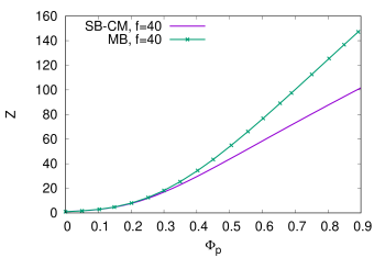
As before, we also determine an interpolation formula for $Z$. In this case, the expression should only apply up to the fluid-solid transition. Therefore, we simply parametrize the results by means of a fifth-order polynomial $Z(\Phi_{p})=1+\sum_{k=1}^{5}a_{k}\Phi^{k}$. The coefficients $a_{k}$ are again reported in Table 3. This interpolation holds up to $\Phi_{p}=0.8$, well within the solid phase (see Sec. V).

It is also interesting to verify whether the polymer equation of state can be reasonably approximated by the hard-sphere one, provided one chooses an appropriate effective hard-sphere radius $R_{c}$. As discussed in Ref. RP-13, , this approximation works nicely for large $f$ in the very dilute limit $\Phi_{p}\to 0$, as the first two virial coefficients $B_{2}$ and $B_{3}$ satisfy the relation $B_{3}/B_{2}^{2}\approx 5/8$, appropriate for hard spheres. The comparison of the finite-density results is performed in the supplementary material. It shows that the identification of large-$f$ star polymers with hard spheres holds only for very dilute solutions. For $f=40$, at $\Phi_{p}=0.15$ the hard-sphere approximation overestimates $Z$ already by 25%.

V Fluid-solid transition for $f=40$

V.1 The solid phase: qualitative predictions

For $f=40$, the analysis of SB models, both using phenomenological WLL-99 and numerically-determinedMP-13 potentials, predicts a solid density window. As a first step, we investigate whether such solid phase also occurs when one uses the MB model. For this purpose we perform canonical simulations, using ordered starting configurations. We generate configurations such that the centers of each star polymer are located on the site of a bcc, fcc, and diamond lattice (the lattice structures that were found to be stable for different values of $f$ in Ref. WLL-99, ), while the arms are randomly located around the centers. Then, the system evolves under a standard Metropolis dynamics (see the supplementary material for details). The volume fractions investigated are $\Phi_{p}=0.8$, $1$, $1.6$, and 2, on cubic simulation boxes with $n=7,8$ elementary cells per side for all three different types of lattice (correspondingly, the number of polymers is $2n^{3}$, $4n^{3}$, and $8n^{3}$, for the bcc, fcc, and diamond case). For all densities, the fcc and diamond lattices are unstable. After $N\approx 2\cdot 10^{3}$ iterations, there is no presence of the original solid structure. On the other hand, the solid bcc structure appears to be stable for $\Phi_{p}=0.8$ and $1.0$. After $10^{5}$ iterations, the star polymers are still approximately located on the sites of a bcc lattice, the molecules only oscillating around the lattice sites. This confirms the (meta)stability of the bcc structure for these volume fractions, so that the fluid-to-solid transition, if present, takes place in the dilute regime, hence at a significantly lower density than that predicted by SB models.

SB models, moreover, predict reentrant melting. WLL-99 The same phenomenon occurs by using the MB model. For $\Phi_{p}=1.6$ and 2 the lattice bcc structure is not stable. After approximately $10^{3}$ iterations, the solid is completely melted. Therefore, we confirm the qualitative picture obtained by using SB models. Quantitative differences are however observed: as we now discuss, the solid phase occurs at lower densities than those predicted by SB models.

V.2 Location of the fluid-solid transition

In order to determine the location of the transition lines, we perform isobaric simulations, using the strategy discussed in Refs. LW-77-78, ; CW-77, ; NVM-08, ; ESVV-13, . We prepare a starting configuration in a box of size $L_{1}\times L_{2}\times L_{3}$ with periodic boundary conditions, such that half of the system is in the solid phase while the second half is in the fluid phase. Then, we let the system evolve at constant pressure. In most of the simulations we keep $L_{1}=L_{2}$ and let $L_{1}$ and $L_{3}$ evolve independently. However, to identify possible orthorombic stable crystal structures we also perform isobaric simulations in which all box dimensions vary independently. Details on the simulations and on the analyses performed are reported in the supplementary material.

We first analyze the SB model in the CM representation. We have performed simulations for $\widetilde{P}=\beta P\hat{R}_{g}^{3}=8.5,10,12.6$, and 17.4, which, according to the equation of state obtained by performing simulations in the fluid phase (disordered starting configuration), should correspond to $\Phi_{p}\approx 0.6,0.64,0.7$, and 0.8, respectively. For $\widetilde{P}=8.5$ the solid part of the system melts, while in all other cases the system freezes. The density stays essentially constant in the simulation: the packing fractions corresponding to the solid and to the metastable fluid phase differ by less than 1%. These results allow us to conclude that the low-density fluid-solid transition occurs at (we report the error on the result in parentheses)

$$\widetilde{P}_{fs}=9.2(8).$$ (17)

The corresponding fluid-solid coexistence density interval $[\Phi_{p,f},\Phi_{p,s}]$ satisfies

$$0.60\mathrel{\hbox to0.0pt{\lower 3.0pt\hbox{$\mathchar 536\relax$}\hss}\raise 2.0pt\hbox{$\mathchar 316\relax$}}\Phi_{p,f}<\Phi_{p,s}\mathrel{\hbox to0.0pt{\lower 3.0pt\hbox{$\mathchar 536\relax$}\hss}\raise 2.0pt\hbox{$\mathchar 316\relax$}}0.64.$$ (18)

At the transition, the solid phase corresponds to a bcc lattice. However, as the pressure is increased we identify other (meta)stable lattice structures. For $\widetilde{P}=12.6$, corresponding to $\Phi_{p}\approx 0.7$, beside the bcc lattice, we also identify two different (meta)stable monoclinic body-centered structures. If we write the vectors identifying the unit cell as

$${\bm{v}}_{1} = (a,0,0),$$

$${\bm{v}}_{2} = (b\tan\phi,b,0),$$

$${\bm{v}}_{3} = (0,0,c),$$ (19)

the two stable structures have $b/a\approx 0.97$, $c/a\approx 1.59$, $|\phi|\approx 14^{\circ}$, and $b/a\approx 0.93$, $c/a\approx 1.66$, $|\phi|\approx 22^{\circ}$. We have not determined which is the most stable structure at this value of the pressure. We have however indications that asymmetric lattice structures become the stable ones as $\widetilde{P}$ increases. For $\widetilde{P}\approx 24$ (corresponding to $\Phi_{p}\approx 0.9$) we find that the bcc lattice structure is unstable. Indeed, if we start the simulation from a system which contains a bcc solid, we end up with a final (body)-centered tetragonal structure, corresponding to $b/a\approx 1$, $c/a\approx 1.4$, $\phi\approx 0$. This tetragonal structure is stable with respect to orthorombic deformations, at variance with what happens for $\widetilde{P}=12.6$. At the latter value of the pressure, tetragonal structures are unstable. Therefore, we predict an additional solid-solid structural transition at $\widetilde{P}_{ss}$ with $12.6<\widetilde{P}_{ss}\mathrel{\hbox to0.0pt{\lower 3.0pt\hbox{$\mathchar 536\relax$}\hss}\raise 2.0pt\hbox{$\mathchar 316\relax$}}24$.

We have also estimated the location of the solid-fluid transition that separates the solid from the high-density fluid phase. Isobaric simulations at $\widetilde{P}=70$, 100, 110, and 120, allow us to estimate a transition for $\widetilde{P}_{sf}=110(10)$. The corresponding coexistence interval $[\Phi_{ps},\Phi_{pf}]$ satisfies $1.27\mathrel{\hbox to0.0pt{\lower 3.0pt\hbox{$\mathchar 536\relax$}\hss}\raise 2.0pt\hbox{$\mathchar 316\relax$}}\Phi_{ps}<\Phi_{pf}\mathrel{\hbox to0.0pt{\lower 3.0pt\hbox{$\mathchar 536\relax$}\hss}\raise 2.0pt\hbox{$\mathchar 316\relax$}}1.66$.

The same analysis has been performed for the MB model, see the supplementary material for details. We observe freezing for $\widetilde{P}=10.9$, 6.6, and 5.0. The packing fraction of the corresponding solid phase is $\Phi_{p}\approx 0.60,0.50,0.46$, respectively. On the other hand, for $\widetilde{P}=3.38$ the system melts: the density of the corresponding fluid is $\Phi_{p}\approx 0.40$. Therefore, in the MB case, the fluid-(bcc) solid transition occurs for

$$\widetilde{P}_{fs}=4.2(8),$$ (20)

and the fluid-solid coexistence density interval satisfies $0.40\mathrel{\hbox to0.0pt{\lower 3.0pt\hbox{$\mathchar 536\relax$}\hss}\raise 2.0pt\hbox{$\mathchar 316\relax$}}\Phi_{p,f}<\Phi_{p,s}\mathrel{\hbox to0.0pt{\lower 3.0pt\hbox{$\mathchar 536\relax$}\hss}\raise 2.0pt\hbox{$\mathchar 316\relax$}}0.46;$ correspondingly we have $Z_{fs}=41(8)$. Note the significant difference between the SB and MB results, both for the pressure and for the densities at coexistence.

In the MB case, we have not performed a detailed analysis of other possible metastable asymmetric lattice structures. We have, however, identified another, at least metastable, lattice structure for $\widetilde{P}=6.6$. The structure is monoclinic with $\phi\approx 12$-$13^{\circ}$, as in the SB case. Therefore, we conclude that the existence of these monoclinic (meta)stable structures is not due the coarse-graining procedure, but that it is a property of the underlying star-polymer system.

Also in the MB case, we have estimated the location of the solid-fluid transition that separates the solid from the high-density fluid phase. We perform isobaric simulations for $\widetilde{P}=55$, 70, 85. For the two largest values of $\widetilde{P}$ the fluid phase is the most stable one, while the bcc crystal is apparently stable for $\widetilde{P}=55$. These results allow us to locate the transition at

$$\widetilde{P}_{sf}=62(8).$$ (21)

The corresponding coexistence interval $[\Phi_{ps},\Phi_{pf}]$ satisfies $1.13\mathrel{\hbox to0.0pt{\lower 3.0pt\hbox{$\mathchar 536\relax$}\hss}\raise 2.0pt\hbox{$\mathchar 316\relax$}}\Phi_{ps}<\Phi_{pf}\mathrel{\hbox to0.0pt{\lower 3.0pt\hbox{$\mathchar 536\relax$}\hss}\raise 2.0pt\hbox{$\mathchar 316\relax$}}1.26$. Note again that the MB results for both the pressure and the coexisting densities are significantly different from those obtained by using the SB model.

VI Polymer size

The residual flexibility of the MB model allows us to investigate the density dependence of the structural intramolecular properties of a single star polymer as the functionality $f$ grows.

The size reduction of the molecules as the density increases can be quantified by means of the average blob radius of gyration $R_{g,b}(\Phi_{p})$ defined in Eq. (11). This quantity differs from the radius of gyration of the microscopic model. Nonetheless, it also provides a measure of the size of the polymer and, therefore, an indication of how stiff the polymer is for different values of $f$. In Fig. 11 we report the adimensional universal combination ${R}_{g,b}(\Phi_{p})/\hat{R}_{g,b}$ ($\hat{R}_{g,b}$ is the zero-density quantity) for the MB model with $f=6$, 12, and 40. The results have been obtained in canonical simulations starting from a disordered configuration. Therefore, they always refer to polymers in the fluid phase. For $f=40$ this phase is unstable for $\Phi_{p}\mathrel{\hbox to0.0pt{\lower 3.0pt\hbox{$\mathchar 536\relax$}\hss}\raise 2.0pt\hbox{$\mathchar 318\relax$}}0.4$. For $f=40$ we have also computed this ratio in the solid bcc phase, without observing any significant difference. For $\Phi_{p}=0.5$ we find $(R_{g,b,\rm fluid}/R_{g,b,\rm solid}-1)\mathrel{\hbox to0.0pt{\lower 3.0pt\hbox{$\mathchar 536\relax$}\hss}\raise 2.0pt\hbox{$\mathchar 316\relax$}}0.1\%$.

Figure 11: Adimensional combination ${R}_{g,b}/\hat{R}_{g,b}$ in the multiblob (MB) model as a function of $\Phi_{p}$, for $f=6$, 12, and 40. The results for $f=40$ are obtained in the fluid phase, which becomes metastable for $\Phi_{p}\mathrel{\hbox to0.0pt{\lower 3.0pt\hbox{$\mathchar 536\relax$}\hss}\raise 2.0pt\hbox{$\mathchar 318\relax$}}0.4$.

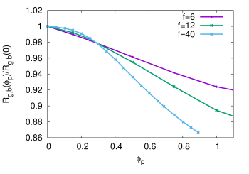
The results for $R_{g,b}$ show the presence of two distinct regimes. For $\Phi_{p}\mathrel{\hbox to0.0pt{\lower 3.0pt\hbox{$\mathchar 536\relax$}\hss}\raise 2.0pt\hbox{$\mathchar 316\relax$}}0.3$, we have the stiff regime. Molecules are stiff and they become more rigid as $f$ increases. For these values of the density, star polymers can be considered as compact hard objects, whose size does not vary with density. This is the regime in which we expect star polymers to be well represented by SB models, which should become more accurate as $f$ increases. However, when the packing fraction exceeds 0.3, one enters a new regime, that we may call compressed regime. This regime is absent for linear polymers: as the density increases, linear polymers simply begin to overlap. Star polymers instead are very compact objects and therefore it is very difficult for them to overlap, especially for large functionalities. Therefore, they start to shrink, reducing the volume effectively occupied by each molecule and the overlap between two different polymers. The compression increases as a function of $f$, as a consequence of the increasing difficulty in overlapping. In this compressed regime, SB models should not be accurate, and indeed, it is exactly for these values of $\Phi_{p}$ that we observe significant differences in the predictions of the osmotic factor $Z$ between the SB and the MB model. MB models are somehow able to describe this compressed phase. However, this is not enough to guarantee that the MB model is accurate, since the strong compression of the molecule might also change significantly the size and shape of the blobs, which are instead assumed to be essentially independent of the density in the multiblob picture. Therefore, even if we are in the dilute regime, it is possible that our MB model loses its accuracy as $f$ increases.

VII Conclusions

In this work we study the thermodynamics and phase behavior of star polymers of different functionalities $f$. We consider polymers with $f=6$ and 12 arms—in this case the behavior resembles that of linear polymers—and stars with $f=40$ arms, which show a more complex behavior, with a solid phase for intermediate values of the density. We use a CG model that captures the star topology, with $f$ blobs representing the polymer arms and one blob corresponding to the star center. We use structurally consistent effective pairwise interactions, which are defined so that the CG model reproduces a set of zero-density distribution functions computed in the microscopic model. Since the determination of the target distributions only requires simulations of two polymers, we are able to consider long chains. Thanks also to the optimality of the chosen microscopic model—we use the Domb-Joyce model at a particular value of the repulsion parameter such that CMP-06 ; DPP-16 the leading finite-length corrections are negligible—we are able to obtain accurate asymptotic estimates of the distribution functions with relatively short polymers (approximately 1000 monomers per arm). As a consequence, our model provides an accurate CG description of star polymers in the universal, large degree-of-polymerization limit. It is important to stress that, as we only consider the universal behavior, we implicitly assume that $L$ is so large that the average monomer density is tiny. In particular, the size of the core should be small compared to $\hat{R}_{g}$. In the Daoud-Cotton model, this requires $L\gg f^{1/2}$: as $f$ increases, larger polymers are needed to observe the universal behavior. This is consistent with the numerical results of Ref. RP-13, , that observed an increase of the finite-size corrections with $f$.

The multiblob (MB) model is used to study the thermodynamics of a solution of star polymers in the dilute and semidilute regime, for $\Phi_{p}\mathrel{\hbox to0.0pt{\lower 3.0pt\hbox{$\mathchar 536\relax$}\hss}\raise 2.0pt\hbox{$\mathchar 316\relax$}}2$. We find that the MB estimates of the pressure coincide with those obtained by using single-blob (SB) models for volume fractions $\Phi_{p}\mathrel{\hbox to0.0pt{\lower 3.0pt\hbox{$\mathchar 536\relax$}\hss}\raise 2.0pt\hbox{$\mathchar 316\relax$}}\Phi_{p,SB}$, where $\Phi_{p,SB}\approx 0.5$ for $f=6,12$ and $\Phi_{p,SB}\approx 0.3$ for $f=40$. Thus, the density interval in which SB models are quantitatively accurate decreases as $f$ increases: At finite density, the SB model becomes less accurate as $f$ increases. This is at variance with what happens in the limit of zero density. For instance, the SB estimates of the virial combination $A_{3}$ become more accurate as $f$ increases.MP-13 ; RP-13

The MB model allows us to study the density dependence of the polymer size. In the very dilute limit polymers are stiff and become more rigid as $f$ increases. In this regime, for large values of $f$ polymers are well represented by hard spheres, i.e., by rigid molecules whose size does not depend on density. This is in agreement with the results of Ref. RP-13, for the ratio $A_{3}/A_{2}^{2}$ that was found consistent with the hard-sphere value 5/8 for $f\to\infty$. The density range in which this occurs is, however, quite small and moreover it decreases as $f$ increases. As $\Phi_{p}$ increases, the soft nature of the polymers becomes more evident, and for $\Phi_{p}\mathrel{\hbox to0.0pt{\lower 3.0pt\hbox{$\mathchar 536\relax$}\hss}\raise 2.0pt\hbox{$\mathchar 318\relax$}}0.3$, we enter a different, compressed regime, in which the ratio $R_{g,b}(\Phi_{p})/\hat{R}_{g}$ decreases significantly with increasing $f$: in this regime, large-functionality star polymers shrink more than linear polymers at the same polymer volume fraction. The origin of this compressed phase can be understood quite easily. As the density increases, the available free space decreases. As it is difficult for polymers to overlap, it is more convenient for them to shrink, an effect that becomes more significant as $f$ increases. In this regime star polymers can no longer be modelled as hard spheres. This significant size change explains why SB models are not accurate for $\Phi_{p}\mathrel{\hbox to0.0pt{\lower 3.0pt\hbox{$\mathchar 536\relax$}\hss}\raise 2.0pt\hbox{$\mathchar 318\relax$}}0.3$: they are simply not able to take this size reduction into account, as they have no internal structure.

We also study the phase diagram for $f=40$. We confirm the presence of an intermediate solid phase, predicted using SB models.WLL-99 However, the fluid-solid transitions occur at lower densities than those predicted by SB models. In particular, the transition separating the solid phase from the low-density fluid phase occurs at $\Phi_{p}\approx 0.4$, while the one between the solid and the high-density fluid phase occurs at $\Phi_{p}\approx 1.2$. The solid phase is therefore in the dilute regime in which star polymers can be viewed as nonoverlapping compressible spheres. In the semidilute regime in which polymers must necessarily overlap, the solid phase is unstable and one observes a dense polymeric fluid. We have also performed a preliminary investigation of the nature of the solid phase. We find several, at least metastable, crystal structures both in the SB and MB model. In the SB case, we also observe a structural transition, separating a low-density bcc phase, and a high density solid phase, in which the stable structure is apparently a centered tetragonal lattice. Further work is needed to completely characterize the nature of the solid phase. In particular, it would be interesting to determine the relative stability of the different crystal structures by a direct comparison of their free energies or enthalpies. This analysis should be feasible using thermodynamic integration methods.

The MB model we have considered here can also be used to determine the phase behavior of mixtures of star polymers with other soft particles, improving the results obtained by using SB representations. ALE-02 ; DLL-02 ; CL-10 ; LCSLZWLR-11 ; LCL-16 It would also be interesting to improve the MB model by increasing the number of interaction sites. This, however, is probably a very hard problem, which requires more sophisticated inversion methods. Finally, it would be interesting to investigate SB compressible models,VBK-10 ; DPP-12-compressible in which the interaction potentials depend on the size of the polymer. In principle, these models are able to describe the compression of the polymer and therefore they might be reasonably accurate also for $\Phi_{p}\mathrel{\hbox to0.0pt{\lower 3.0pt\hbox{$\mathchar 536\relax$}\hss}\raise 2.0pt\hbox{$\mathchar 318\relax$}}0.3$. Work in this direction is in progress.

Supplementary material

In the supplementary material we report numerical data and details on the computations we performed. In particular: i) we compare integral-equation and Monte Carlo results for SB models; ii) we compare the MB results for the pressure with theoretical predictions; iii) we define the Domb-Joyce model and its asymptotic behavior; iv) we give some algorithmic details on the simulations of the multiblob model; v) we provide a detailed description of our results for the determination of the transitions separating the fluid phases from the intermediate solid phase for star polymer systems with 40 arms.

Appendix A Inversion procedure for the intermolecular potentials.

The determination of the intermolecular potentials becomes increasingly difficult as $f$ increases. For $f=6$ and 12 the standard IBI method Schommers-83 ; MP-02 ; RPMP-03 or a small variant thereof works reasonably. For $f=40$ instead we have not able to use the IBI method and we have used an ad hoc procedure, close in spirit to the approach of Ref. AB-01, . Below we give a few details of the approach.

A.1 Low-functionality stars: $f=6$ and $f=12$

For $f=6$ the IBI method Schommers-83 ; MP-02 ; RPMP-03 used for the intramolecular interactions still works reasonably, provided one uses an appropriate mixing parameter $a$ (we use $a\approx 0.1$-0.2) as in Eq. (10). We first perform a set of IBI iterations in which we fix $\widetilde{V}_{ca}(b)=\widetilde{V}_{cc}(b)=\widetilde{V}_{aa}(b)$ and determine $\beta\widetilde{V}_{aa}(b)$ by requiring the CG model to reproduce $\beta W_{aa}^{FM}(b)$. Once this is done, we perform a second set of IBI iterations in which we vary independently $\widetilde{V}_{aa}(b)$ and $\widetilde{V}_{ca}(b)$, setting at each step $\widetilde{V}_{cc}(b)=\widetilde{V}_{ca}(b)$. We stop when the CG model reproduces the full-monomer arm-arm and center-arm potentials of mean force. Finally, we perform IBI iterations, varying independently the three potentials, until we reproduce all potentials of mean force. In total, we perform 300 iterations.

For $f=12$ the IBI method Schommers-83 ; MP-02 ; RPMP-03 works, although not straightforwardly. The main reason for the failure of the standard IBI method is the presence of long tails, which extend up to $4\hat{R}_{g}$ (see the discussion at the end of Sec. II.2), in the mean-force potentials. Indeed, if we use Eq. (10) with the distributions $P$ replaced by $e^{-\beta W}$, in a few iterations also the intermolecular potentials $\widetilde{V}$ develop a similar tail, which increases with the number of iterations. Such a tail is clearly unphysical. We expect the potentials to have a range of the order of a few blob radii of gyration. As $\hat{r}_{g}\approx 0.5\hat{R}_{g}$, we expect the potentials to be small beyond, say, $2\hat{R}_{g}$.

To avoid the appearance of these tails, we have modified the IBI procedure, introducing an appropriate mixing function $a_{ij}(b)$. We therefore perform a set of iterative steps in which the potentials are updated using

$$\widetilde{V}_{(n+1),ij}(b)=\widetilde{V}_{n,ij}(b)-a_{ij}(b)[W_{n,ij}^{CG}(b)-W^{FM}_{ij}(b)].$$ (22)

We choose Gaussian functions

$$a_{ij}(b)=Ae^{-b^{2}/\sigma^{2}},$$ (23)

with the same amplitudes $A$ and widths $\sigma$ for all potentials. We use $A=0.2$ and $\sigma=1.8$. In practice, we proceed as follows. We start the IBI procedure from the $f=6$ potentials and perform several iterations (22), updating all potentials at each step. Once the potentials of mean force are approximately reproduced, we perform some standard IBI iterations with a constant mixing parameter $a$. We start with $a=0.1$ and then we reduce it, taking $a=0.05$ in the last set of iterations. The total number of IBI iterations is 250.

A.2 High-functionality stars: $f=40$

Figure 12: A typical configuration for the determination of the arm-arm potential of mean force. We fix the distance $r$ between two arbitrary blobs and compute the total intermolecular potential energy. The summation contains contributions $\widetilde{V}_{aa}(r^{\prime})$, in which $r^{\prime}$ (the distance between different pairs of blobs) varies significantly (significant contributions are obtained up to $r^{\prime}$ of the order of $4\hat{R}_{g}$).

The determination of the intermolecular potentials $\beta\widetilde{V}_{ij}$ for $f=40$ has been more difficult than for $f=6,12$, and deserves a separate discussion. In this case the IBI method does not work, even in the modified form (22). To understand the origin of the problems, we should first realize that, in the computation of the intermolecular potential energy, there are $f^{2}$ contributions depending on $\widetilde{V}_{aa}$, $2f$ contributions depending on $\widetilde{V}_{ca}$, and only one term depending on $\widetilde{V}_{cc}$. The presence of this hierarchy implies that even a small change of $\widetilde{V}_{aa}$ gives rise to a significant change of all $\beta W_{ij}$, so that such potential should be only slightly changed at each step. The second problem stems from an intrinsic property of the IBI method. At each step, the potential at distance $b$ is corrected by using the difference $W_{(n,ij)}^{CG}(b)-W^{FM}_{ij}(b)$ at the same value of $b$, see Eq. (22). Implicitly, this assumes that, if we only change the potential in a tiny region around $b=b_{0}$, the potentials of mean force change significantly only in a small region close to $b=b_{0}$. This assumption does not hold in our case. Indeed, the mean force potentials are computed from Eq. (4), that is fixing the distance $r$ between two blobs and then averaging $e^{-\beta U_{\rm inter}}$ over the positions of all other blobs. The distance among all other blobs varies among all possible values in the range of the potentials, see Fig. 12. This means that $W_{aa}(b)$ for $b=b_{0}$ depends on the value of $\widetilde{V}_{aa}(b)$ for any value $b$, as it gets contributions from $f^{2}$ pair of blobs whose distance is quite different from that of the two blobs we have kept fixed. The problem is less severe, but still present, for the center-arm potential that gives $2f$ contributions to the calculation of $W_{ca}(b)$, while it is not present for $\widetilde{V}_{cc}(b)$.

As the IBI method cannot be used, we adopt a different strategy, close in spirit to the approach of Ref. AB-01, . We choose appropriate parametrizations of the potentials and optimize the coefficients, so as to obtain the best possible agreement between the potentials of mean force computed in the full-monomer and CG models. We start from a set of Gaussian potentials $\beta\widetilde{V}_{ij}^{(0)}(b)=A_{ij}\exp[-(b/\sigma_{ij})^{2}]$, fixing $A_{ij}$ and $\sigma_{ij}$ to some reasonable values — we are guided by the results for $f=6$ and 12 — so that every potential of mean force $\beta W_{ij}(b)$ computed in the CG model is not very different from its full-monomer counterpart in the relevant region, i.e., for the values of $b$ where $\beta W_{ij}(b)\mathrel{\hbox to0.0pt{\lower 3.0pt\hbox{$\mathchar 536\relax$}\hss}\raise 2.0pt\hbox{$\mathchar 316\relax$}}10$. Then, keeping the center-arm and center-center potentials fixed, we perform systematic changes of $A_{aa}$ and $\sigma_{aa}$ in order to improve the agreement between the CG and FM estimates of $\beta W_{aa}(b)$. We stop the procedure when $\beta W_{aa}^{FM}(b)$ is roughly reproduced in the CG model. After this optimization, we compute the other potentials of mean force, finding that both $\beta W_{ca}^{CG}(b)$ and $\beta W_{cc}^{CG}(b)$ significantly overestimate the corresponding full-monomer quantity. At this point, we optimize the center-arm potential. We change the functional form of the center-arm potential and parametrize it as $\beta\widetilde{V}_{ca}^{(0)}(b)=A_{ca}\exp[-(b/\sigma_{ca})^{2}](1-k_{ca}b^{2})$. The introduction of the term proportional to $k_{ca}$ makes it possible for the potential to have an attractive tail. The parameters $A_{ca}$, $\sigma_{ca}$, and $k_{ca}$ are then optimized in such a way to roughly reproduce $\beta W_{ca}^{FM}(b)$. The arm-arm potential of mean force $\beta W_{aa}^{CG}(b)$ changes: it slightly underestimates $\beta W_{aa}^{FM}(b)$ at the end of the procedure. In particular, tails appear to be understimated. At this point we optimize again the arm-arm potential, choosing a slightly different parametrization: $\beta\widetilde{V}_{aa}(b)=A_{aa}\exp[-(b/\sigma_{aa})^{t}]$. The exponent $t$ is introduced to obtain a better agreement for $b\mathrel{\hbox to0.0pt{\lower 3.0pt\hbox{$\mathchar 536\relax$}\hss}\raise 2.0pt\hbox{$\mathchar 318\relax$}}2$. The parameters $t$, $A_{aa}$, and $\sigma_{aa}$ are again optimized. At the end of the procedure, we obtain $t=1.86$—the potential decays slightly slower than a Gaussian—and the two potentials of mean force, $\beta W_{aa}(b)$ and $\beta W_{ca}(b)$, are accurately reproduced in the relevant region. Only $\beta W_{cc}^{CG}(b)$ differs from the full-monomer target quantity. At this point we change $\widetilde{V}_{cc}(b)$ using Eq. (22) and setting $a_{cc}=1$. Since the contribution of this potential to the total intermolecular potential energy is of order 1, within our target precision (1%) this change does not modify the arm-arm and the center-arm mean-force potentials.

The potentials of mean force for the full-monomer and CG models with $f=40$ are compared in Fig. 4. As it can be seen, the CG model with the obtained potentials reproduces quite accurately the target distributions.

It is interesting to discuss the accuracy of the results. If we vary $\widetilde{V}_{aa}(b)$ by 1%, i.e., we consider either $1.01\widetilde{V}_{aa}(b)$ or $0.99\widetilde{V}_{aa}(b)$, keeping $\widetilde{V}_{ca}(b)$ and $\widetilde{V}_{cc}(b)$ fixed, the potentials of mean force $W_{aa}^{CG}(b)$ and $W_{ca}^{CG}(b)$ change at most by 1%, which is the accuracy with which we reproduce the full-monomer potentials of mean force. Analogously, if we change $\widetilde{V}_{ca}(b)$ by 1%, $W_{aa}^{CG}(b)$ and $W_{ca}^{CG}(b)$ change by less than 0.6%. Therefore, we conclude that $\widetilde{V}_{aa}(b)$ and $\widetilde{V}_{ca}(b)$ are determined with an error of approximately 1%. As for the potential $\widetilde{V}_{cc}(b)$, its value is strictly correlated to that of $\widetilde{V}_{aa}(b)$ and $\widetilde{V}_{ca}(b)$. Indeed, when we change one of these two potentials by 1%, we should change $\widetilde{V}_{cc}(b)$ by 3-4% to guarantee that $W_{cc}^{FM}(b)$ is reproduced. Therefore, we estimate an error of at most 5% on $\widetilde{V}_{cc}(b)$.

Appendix B Supplementary material

B.1 Summary

In this supplementary material we report numerical data and details on the computations we performed. In particular: i) we compare integral-equation and Monte Carlo results for SB models; ii) we compare the MB results for the pressure with theoretical predictions; iii) we define the Domb-Joyce model and its asymptotic behavior; iv) we give some algorithmic details on the simulations of the multiblob model; v) we provide a detailed description of our results for the determination of the transitions separating the fluid phases from the intermediate solid phase for star polymer systems with 40 arms.

B.2 Integral equations

	$\Phi_{p}=0.25$		$\Phi_{p}=0.80$		$\Phi_{p}=2.0$
$f$	RY	MC	RY	MC	RY	MC
6	2.146	2.143	5.832	5.846	14.626	14.617
12	3.601	3.621	14.573	14.707	40.450	40.630
40	11.781	11.850	87.595	86.930	—	—

Table 4: Compressibility factor $Z(\Phi_{p})$ for the SB model in the CM representation, for $f=6$, 12 and 40. We compare RY and MC results. The results for $\Phi_{p}=0.80$ and $f=40$ are obtained in the metastable fluid phase.

In the integral-equation approach one determines the pair correlation function $h(r)$ and the direct correlation function $c(r)$, by requiring the validity of the Ornstein-Zernike relation HMD-suppl

$$\hat{h}(k)=\hat{c}(k)+\rho\hat{c}(k)\hat{h}(k)$$ (24)

(here $\hat{f}(k)$ is the (three-dimensional) Fourier transform of $f(r)$) and of a closure relation. We use the Rogers-Young closure defined by RY-84-suppl

$$g(r)=e^{-\beta V(r)}\left[1+{\exp[(h(r)-c(r))f(r)]-1\over f(r)}\right],$$ (25)

where the function $f(r)$ is given by

$$f=1-e^{-\chi r}.$$ (26)

The closure relation depends on the parameter $\chi$ which is fixed by requiring thermodynamic consistency for the pressure, i.e., the equivalence of the virial and of compressibility route.HMD-suppl

This closure has been extensively used in the analysis of single-blob (SB) models. LLWAJAR-98-suppl ; WLL-99-suppl ; MP-13-suppl To verify its accuracy we have compared its predictions for the compressibility factor $Z$ with Monte Carlo results for different values of $\Phi_{p}$. The results are reported in Table 4. In all cases, differences are less than 1%.

B.3 Comparison of the thermodynamic results with other predictions

B.3.1 Renormalization-group predictions

Here we wish to compare our results for the osmotic factor $Z$ with the renormalization-group predictions of Ref. CBMF-86-suppl, (they are reviewed and compared with experiments in Refs. DRF-90-suppl, ; MBLFG-93-suppl, ). These predictions are obtained using the standard dimensional expansion in powers of $\epsilon=4-d$, where $d$ is the space dimension. The result is expressed in terms of the adimensional concentration

$$\overline{c}=B_{2}{N_{p}\over V}={3\over 4\pi}A_{2}\Phi_{p},$$ (27)

where $B_{2}$ is the second virial coefficient and $N_{p}$ is the number of star polymers in the box of size $V$. At first order in $\epsilon$, the compressibility factor $Z$ is

$$Z=1+\overline{c}\left(1-{\epsilon\over 16\overline{c}^{2}}I(\overline{c})\right),$$ (28)

where

$$I(\overline{c}) = \int_{0}^{\infty}y^{3}dy\left\{\vphantom{1\over 2}\ln[1+4\overline{c}g(y)]\right.$$ (29)

$$\quad\left.-{4\overline{c}g(y)\over 1+4\overline{c}g(y)}-8\overline{c}^{2}g(y)^{2}\right\},$$

$$g(y) = {1\over y^{2}}+{h(y)\over y^{4}}\left[1+{1\over 2}(f-1)h(y)\right],$$ (30)

$$h(y) = e^{-y^{2}/f}-1.$$ (31)

This expression is supposed to be accurate only for small values of $f$, say $f\mathrel{\hbox to0.0pt{\lower 3.0pt\hbox{$\mathchar 536\relax$}\hss}\raise 2.0pt\hbox{$\mathchar 316\relax$}}6$. For larger values, the coefficients of the expansion increase significantly, so that one-loop results are not predictive.DRF-90-suppl ; MBLFG-93-suppl If $Z_{MB}$ is the multiblob (MB) Monte Carlo result and $Z_{RG}$ is the expression reported above with $\epsilon=1$, we obtain for $f=6$:

$\Phi_{p}=0.15$:	$\qquad Z_{MB}=1.64$	$\qquad Z_{RG}=1.73$,
$\Phi_{p}=0.25$:	$\qquad Z_{MB}=2.18$	$\qquad Z_{RG}=2.36$,
$\Phi_{p}=0.50$:	$\qquad Z_{MB}=3.93$	$\qquad Z_{RG}=4.16$,
$\Phi_{p}=0.75$:	$\qquad Z_{MB}=5.92$	$\qquad Z_{RG}=6.14$,
$\Phi_{p}=1.00$:	$\qquad Z_{MB}=8.13$	$\qquad Z_{RG}=8.23$.

The agreeement is reasonable, with differences that are at most of 6%. We also compared the multiblob results with Eq. (28) for $f=12$: in this case discrepancies are very large, of the order of 50%, confirming the unreliability of the $\epsilon$-expansion for large functionalities.

For larger values of $\Phi_{p}$ the renormalization-group expression (28) is not predictive. Indeed, for large $\overline{c}$ we obtain

$$Z=1+\overline{c}\left\{1+{\epsilon\over 4}\left[\log(4\overline{c})+a(f)\right]\right\},$$ (32)

($a(f)\approx 2.7$ for $f=6$), which differs from the expected $Z\sim\overline{c}^{1.311}$. The correct behavior can be obtained by exponentiating the logarithmic term and noting that $(2-d\nu)/(d\nu-1)\approx\epsilon/4+O(\epsilon^{2})$. However, there is no unambiguous way to obtain the prefactor.

B.3.2 Star polymers as hard spheres

It is interesting to verify whether there exists a range of densities in which star polymers can be modelled as hard spheres with an effective radius $R_{c}$. We fix $R_{c}$ by requiring $Z$ to be exactly reproduced for $\rho_{p}\to 0$ at order $\rho_{p}$, where $\rho_{p}$ is the polymer number density. Therefore, we require

$$Z_{\rm pol}\approx 1+A_{2}\hat{R}_{g}^{3}\rho_{p}=1+{16\pi\over 3}R_{c}^{3}\rho_{p},$$ (33)

which implies

$${R_{c}\over\hat{R}_{g}}=\left({16\pi\over 3A_{2}}\right)^{1/3}.$$ (34)

We then compare the hard-sphere equation of state (we use the Carnahan-StarlingHMD-suppl expression) with the MB results. For $\Phi_{p}=0.15$ we obtain:

$f=6$:	$\qquad Z_{HS}=1.72$	$\qquad Z_{MB}=1.64$;
$f=12$:	$\qquad Z_{HS}=2.53$	$\qquad Z_{MB}=2.11$;
$f=40$:	$\qquad Z_{HS}=6.00$	$\qquad Z_{MB}=4.79$.

Even for such a small density, the hard-sphere equation of state is not accurate. Even worse, the accuracy decreases as $f$ increases: the density interval in which star polymers can be considered as hard spheres decreases as $f$ increases.

B.4 Domb-Joyce model

The atomistic (full-monomer) results have been obtained by using the lattice Domb-Joyce model.DJ-72-suppl A linear polymer chain of length $L$ is represented by a lattice random walk $\{{\bm{r}}_{1},\ldots,{\bm{r}}_{L}\}$ on a cubic lattice with $|{\bm{r}}_{i}-{\bm{r}}_{i+1}|=1$. An effective local repulsion is introduced by penalizing self-intersections. Chains are indeed averaged with weight $e^{-wE}$, where $w$ is a free parameter that plays the role of inverse temperature and the energy $E$ is the number of self-intersections,

$$E[\{{\bf r}_{i}\}] = \sum_{1\leq i<j\leq L}\delta({\bm{r}}_{i},{\bm{r}}_{j}),$$ (35)

where $\delta({\bm{r}},{\bm{s}})=1$ if ${\bm{r}}={\bm{s}}$ and $\delta({\bm{r}},{\bm{s}})=0$ otherwise. The athermal self-avoiding walk model is obtained as the limit $w\to\infty$ of the Domb-Joyce model. Self-intersections are forbidden and only walks such that ${\bm{r}}_{i}\not={\bm{r}}_{j}$ are sampled. The model can be generalized to star polymers.HNG-04-suppl ; RP-13-suppl A star polymer with $f$ arms and degree of polymerization $Lf$ is represented by $f$ random walks of length $L$ on a cubic lattice that have a common origin, i.e. by the set of lattice points $\{{\bf r}_{\alpha,i}\}$, $\alpha:1,\ldots,f$, $i:1,\ldots,L$, with ${\bf r}_{1,1}={\bf r}_{2,1}=\ldots={\bf r}_{f,1}$ and $|{\bf r}_{\alpha,i}-{\bf r}_{\alpha,i+1}|=1$. The corresponding energy is

$$E[\{{\bf r}_{\alpha,i}\}] = \sum_{1\leq\alpha<\beta\leq f}\sum_{i,j}\delta({\bf r}_{\alpha,i},{\bf r}_{\beta,j})$$ (36)

$$+\sum_{\alpha}\sum_{1\leq i<j\leq L}\delta({\bf r}_{\alpha,i},{\bf r}_{\alpha,j}).$$

We have considered here a single chain. The generalization to several interacting chains (this is needed for the computation of the potentials of mean force) is completely analogous. For any $w>0$, the Domb-Joyce model describes polymers under good-solvent conditions for large enough values of $L$. However, the asymptotic limit is observed for values of $L$ that significantly depend on $w$. Therefore, $w$ represents a crucial parameter that should be optimized to obtain asymptotic results with the least computational effort.

To make the discussion quantitative, consider a generic large-scale adimensional quantity $A$, which depends on $L$, $f$, and $w$. For large $L$, renormalization group predicts

$$A(L,f,w)=A^{*}(f)+a_{A}(f,w)/L^{\Delta}+b_{A}(f,w)/L^{\Delta_{2}}+\ldots$$ (37)

where $A^{*}(f)$ is universal, i.e. model-independent: for any $w>0$ the limiting value depends only on the functionality $f$. The exponent $\Delta$ is also universal [simulations of linear SAWs give Clisby-10-suppl $\Delta=0.528(12)$]. The amplitudes $a_{A}(f,w)$ and $b_{A}(f,w)$ depend instead on $w$. However, given two different observables $A$ and $B$, the amplitude ratios $a_{A}(f_{1},w)/a_{B}(f_{2},w)$ are model independent.AA-80-suppl

In order to obtain the universal leading quantity $A^{*}(f)$ with the least computational effort, it is convenient to choose $w$ so that $a_{A}(w,f)=0$. For this particular value $w^{*}$, convergence is faster. Note also that, if $a_{A}(w^{*},f_{1})=0$ for a specific quantity $A$ and functionality $f_{1}$, we have $a_{B}(w^{*},f_{2})=0$ for any quantity $B$ and any $f_{2}$, because of the universality of the amplitude ratios. Therefore, for $w=w^{*}$ convergence is faster for any observable and value of $f$ (this was explicitly checked in Ref. RP-13-suppl, ). The optimal value $w^{*}$ has been determined in several papers using linear polymers. BN-97-suppl ; CMP-06-suppl ; DP-16-suppl ; Clisby-17-suppl The simulations we present here were performed taking $w=0.5058$, which is close to the most recent estimate $w^{*}=0.4828(13)$ of Ref. Clisby-17-suppl, .

The Domb-Joyce model for linear polymers can be efficiently simulated using the pivot algorithm.MS-88-suppl ; Kennedy-02-suppl ; CMP-06-suppl For star polymers an efficient algorithm is discussed in Ref. RP-13-suppl, , which combines pivot moves with a new set of moves that speed up the simulation close to the center of the star.

B.5 Simulations of the coarse-grained multiblob model

In all simulations of the coarse-grained model we use a simple Metropolis dynamics. In the multiblob case we consider three different types of displacement moves:

• displacement of an arm blob;

• displacement of a center blob;

• rigid displacement of a single star.

In all cases, the new position is chosen uniformly in a cube centered in the old blob (or molecule) position. The linear size $(2\Delta)$ of the cube is chosen to guarantee an average acceptance rate of approximately 40-50% and turns to be little dependent on the density of the system. For $f=40$, in the analysis of the freezing transition, we use $\Delta=0.4\hat{R}_{g}$, $0.05\hat{R}_{g}$, $0.1\hat{R}_{g}$ for the moves of type i), ii), and iii), respectively. In the same simulations we also perform random rotations of the star around the central blob. Their average acceptance is approximately 40%, with a small density dependence. This relatively large acceptance is probably due to the fact that the stars do not overlap significantly at the densities we have considered.

In the following we report multiblob results for $f=40$ in terms of iterations. In one iteration we attempt $Nf/2$ moves of type i), $N$ moves of type ii), $N$ moves of type iii), and $N$ random rotations, where $N$ is the number of molecules in the system. In all cases the molecule (and also the arm blob for moves i) is randomly chosen at each step. In the fluid phases particle diffuse quite rapidly. For $f=40$ the diffusion coefficient for the centers of mass of the stars is $(0.047\hat{R}_{g})^{2}$ per iteration at $\widetilde{P}=85$ (high-density fluid phase) and $(0.063\hat{R}_{g})^{2}$ per iteration at $\widetilde{P}=3.38$ (low-density fluid phase).

In the isobaric simulations we also attempt to change the box dimensions $L_{i}$ (we consider parallelepipedal boxes of size $L_{1}\times L_{2}\times L_{3}$). We perform Metropolis moves proposing

$$\ln L^{\prime}_{i}=\ln L_{i}+\Delta_{L}(r-0.5),$$ (38)

where $r$ is a uniform random number in $[0,1]$ and $\Delta_{L}$ is chosen to have an acceptance of 50%. We perform 5 volume-change trials every iteration.

Single-blob simulations are done in a similar fashion. We perform random displacements of the molecules, choosing the linear size $(2\Delta)$ of the displacement cube so that the average acceptance is approximately 40-50%. For $\widetilde{P}=8.5$ we take $\Delta=0.12\hat{R}_{g}$, while for $\widetilde{P}=120$, we take $\Delta=0.02\hat{R}_{g}$. Note that here $\Delta$ significantly depends on density.

B.6 Freezing transition

B.6.1 Technical details

We give here some technical details on the analysis of the stability of the solid structures. To understand whether the fluid or the solid phase is the most stable one, we consider starting configurations such that half of the system is in the solid phase, while the second half is fluid. Then, we let the system evolve at constant pressure. In most of the simulations we consider boxes of size $L_{1}\times L_{1}\times L_{3}$, updating independently $L_{1}$ and $L_{3}$, which should also allow us to observe, at least in principle, cubic-to-tetragonal transitions. If the stable phase is the fluid one, the solid melts. In the opposite case, at the end of the simulation all molecules belong to a crystal structure.

Let us now define more precisely the starting configurations that have been used in most of the simulations. We consider a box of size $L_{1}\times L_{1}\times L_{3}$ and a centered tetragonal lattice with primitive lattice vectors

$${\bm{u}}_{1} = \left({a\over 2},{a\over 2},{c\over 2}\right),$$

$${\bm{u}}_{2} = \left({a\over 2},-{a\over 2},{c\over 2}\right),$$

$${\bm{u}}_{3} = \left({a\over 2},{a\over 2},-{c\over 2}\right).$$ (39)

The bcc lattice is obtained for $c=a$. The solid part of the system is a lattice of size $L_{1}=na$, $L_{3}^{(s)}=mc$, with $L_{3}^{(s)}=L_{3}/2$. The total number of molecules belonging to the solid is therefore $N_{\rm sol}=2n^{2}m$. To specify fully the structure, we must fix the aspect ratio $c/a$ and the lattice spacing $a$. In more detail, if ${\bm{r}}_{0}^{(\alpha)}=(x^{(\alpha)},y^{(\alpha)},z^{(\alpha)})$, $\alpha=1,\ldots,4n^{2}m$, are the coordinates of the centers of the polymers, we set at time $t=0$ (starting configuration)

$${\bm{r}}_{0}^{(\alpha)}(t=0)=(k_{1}a,k_{2}a,k_{3}c),$$ (40)

for $\alpha=1+k_{1}+k_{2}n+k_{3}n^{2}$, where $0\leq k_{1}<n$, $0\leq k_{2}<n$, $0\leq k_{3}<m$, and

$${\bm{r}}_{0}^{(\alpha)}(t=0)=(k_{1}a,k_{2}a,k_{3}c)+(a/2,a/2,c/2),$$ (41)

for $\alpha=1+k_{1}+k_{2}n+k_{3}n^{2}+N_{\rm sol}/2$, where $k_{1},k_{2},k_{3}$ vary as before. For the fluid ($N_{\rm sol}+1\leq\alpha\leq 2N_{\rm sol}$) instead, we choose $x^{(\alpha)}$ and $y^{(\alpha)}$ randomly in $[0,L_{1}]$ and $z^{(\alpha)}$ in $[L_{3}/2,L_{3}]$. Once the centers of the polymers are fixed, the arms are positioned randomly around them. The same procedure is applied in the SB case: here the vectors ${\bm{r}}_{0}^{(\alpha)}$ are the positions of the CG molecules.

Before performing the isobaric simulations, we perform two short canonical thermalization runs. In the first one, the positions of the centers are kept fixed, while the arms are randomly displaced (20-50 iterations; in each iterations we only try moves of type i), see Sec. B.5). In the second one, we still do not move the centers of the molecules belonging to the solid; all other blobs are instead randomly displaced (20-50 iterations). The resulting configuration is the starting one for the isobaric simulation. Of course, in the SB case only the second run is performed.

To verify whether the system freezes, i.e., to verify whether the solid phase is the stable one, we proceed as follows. First, we introduce adimensional coordinates

$${\bm{s}}^{(\alpha)}=\left({nx^{(\alpha)}\over L_{1}},{ny^{(\alpha)}\over L_{1}},{2my^{(\alpha)}\over L_{3}}\right),$$ (42)

($n$ and $m$ refer to the number of lattice cells in the $x$ and $z$ directions, respectively, see the definition of the starting configuration), so that the $x$ and $y$ components of ${\bm{s}}^{(\alpha)}$ vary between 0 and $n$, while the $z$ component varies between 0 and $2m$. If the crystal has not melted in the simulation, the positions of the polymers with $\alpha\leq N_{\rm sol}$ should be close to a lattice structure. However, since we use periodic boundary conditions, a global translation is possible. Therefore, we introduce

$${\bm{a}}_{\alpha} = (k_{1},k_{2},k_{3})\quad\alpha=1+k_{1}+k_{2}n+k_{3}n^{2}$$

$${\bm{a}}_{\alpha} = (k_{1}+1/2,k_{2}+1/2,k_{3}+1/2)$$

$$\hphantom{(k_{1},k_{2},k_{3})\quad}\alpha=1+k_{1}+k_{2}n+k_{3}n^{2}+N_{\rm sol}/2$$

($k_{1}$, $k_{2}$, and $k_{3}$ vary as before) and then fix a translation vector ${\bm{c}}$ by minimizing

$$\sum_{\alpha}\left({\bm{s}}^{(\alpha)}-{\bm{a}}_{\alpha}-{\bm{c}}\right)^{2},$$ (44)

where we sum over all molecules in the solid portion of the system which do not belong to the fluid-solid interface, i.e., we do not consider the molecules with $k_{3}=0$ or $k_{3}=m-1$. As usual, we take into account the periodic boundary conditions by using the minimum image convention. Once ${\bm{c}}$ has been determined, we define the lattice positions

$${\bm{b}}_{\alpha} = {\bm{a}}_{\alpha}+{\bm{c}}\qquad\qquad\qquad 1\leq\alpha\leq N_{\rm sol}$$ (45)

$${\bm{b}}_{\alpha} = {\bm{a}}_{\beta}+{\bm{c}}+(0,0,m)\qquad N_{\rm sol}+1\leq\alpha\leq 2N_{\rm sol},$$

with $\beta=\alpha-N_{\rm sol}$. For each of the sites of this lattice, we determine the distance from the closest polymer center:

$$d_{\gamma} = \min_{\alpha}|{\bm{s}}^{(\alpha)}-{\bm{b}}_{\gamma}|.$$ (46)

Finally, we define $N_{m}(\epsilon)$, which gives the number of sites for which such distance is less than $\epsilon$. We distinguish between the solid and fluid phase, defining

$$N_{ms}(\epsilon)={1\over N_{p}}\sum_{\gamma\leq N_{\rm sol}}\theta(\epsilon-d_{\gamma})$$

$$N_{mf}(\epsilon)={1\over N_{p}}\sum_{\gamma>N_{\rm sol}}\theta(\epsilon-d_{\gamma}),$$ (47)

where $N_{p}$ is the total numer of molecules. For a bcc or a centered tetragonal lattice, the nearest-neighbor distance is $\sqrt{3}/2\approx 0.866$, hence $\epsilon$ should be taken at least less that 0.4 to obtain meaningful results. In the following, we shall report results using $\epsilon=0.2$.

B.6.2 The single-blob model

Figure 13: Plot of $N_{ms}(\epsilon)$ and of $N_{mf}(\epsilon)$ as a function of the number $t$ of iterations. Top: $\widetilde{P}=12.6$; middle: $\widetilde{P}=10.0$; bottom: $\widetilde{P}=8.5$. Here $\epsilon=0.2$. Results for $864$ and 1296 molecules (for $\widetilde{P}=10$ and 8.5 only). For $\widetilde{P}=12.6$ and 10, the solid is the stable phase; for $\widetilde{P}=8.5$ the stable phase is fluid.

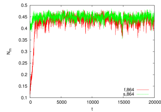
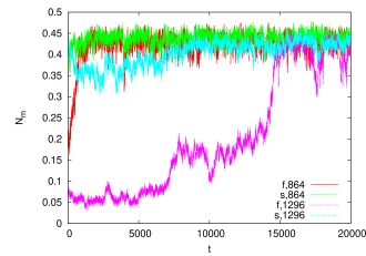
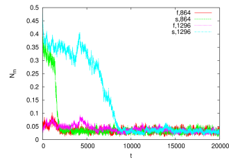
To determine the solid-fluid boundary we first perform preliminary canonical simulations for several values of $\Phi_{p}$, starting from a bcc crystal structure with 250 molecules. We find that the bcc structure is apparently stable for $\Phi_{p}\mathrel{\hbox to0.0pt{\lower 3.0pt\hbox{$\mathchar 536\relax$}\hss}\raise 2.0pt\hbox{$\mathchar 318\relax$}}0.7$: no evidence of melting is observed for runs consisting of $10^{4}$ iterations (in one iteration we try to randomly move all molecules). To identify the density range in which the solid phase is stable, we perform isobaric runs, starting from mixed (solid-fluid) configurations, as described in Sec. B.6.1. We consider an $L_{1}\times L_{1}\times L_{3}$ box and we generate three different configurations with $c=a$ (bcc lattice), $n=m=6$ (the total number of particles is 864) and $\Phi_{p}=0.6$, 0.7, 0.8. Since the equation of state obtained using integral equations predicts $\widetilde{P}\approx 8.5$, 12.6, and 17.4 ($\widetilde{P}=\beta P\hat{R}_{g}^{3}$) for these packing fractions, the generated configurations are used to start the runs at $\widetilde{P}=8.5$, 12.6, and 17.4, respectively. We find that the solid is the stable phase for the two largest values of $\widetilde{P}$, while the stable phase is fluid for $\widetilde{P}=8.5$. This is evident from Fig. 13, where we report $N_{mf}(\epsilon)$ and $N_{ms}(\epsilon)$ for $\widetilde{P}\approx 8.5$ and 12.6. For the smallest value of the pressure the number of molecules that are close to the crystal structure decreases rapidly, while the opposite occurs for the largest value of $\widetilde{P}$. To improve the estimate of the pressure at the transition, we perform a simulation at $\widetilde{P}=10.0$, again with 864 particles: the solid structure is stable, see Fig. 13.

We also study the size dependence of the results. For this purpose we repeat the runs for $\widetilde{P}=10$ and 8.5 with a larger number of particles. We start the simulation from a mixed configuration in which the solid is a bcc lattice with $n=6$, $m=9$. The total number of particles is 1296. The conclusions are identical, see Fig. 13.

Figure 14: Plot of $L_{3}/L_{1}$ as a function of the number $t$ of iterations (we compute this quantity every 10 iterations) for starting configurations that differ in the value of $r_{\rm start}=c/a$. Results for systems of 1024 molecules ($n=m=8$) and $\widetilde{P}=12.6$.

Figure 15: Plots of $\phi$ (in degrees) as a function of the number $t$ of iterations (we estimate $\phi$ every 200 iterations): red points correspond to systems with unit cell given in Eq. (48), green points to systems with unit cell given in Eq. (49). Results for systems of 1024 molecules ($n=m=8$) and $\widetilde{P}=12.6$. Top: run with $r_{\rm start}=1.75$; bottom: run with $r_{\rm start}=1.5$.

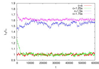
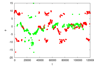
We also study if it is possible to have a tetragonal solid phase. For this purpose we perform five runs at $\widetilde{P}=12.6$, using different solid starting configurations. The starting configuration is a (body) centered tetragonal lattice with $n=m=8$ (1024 molecules), with five different values of $r_{\rm start}=c/a$. The size $a$ is fixed by requiring $\Phi_{p}=0.7$ (which is the equilibrium value of the packing fraction for such value of the pressure). Then, we monitor the ratio $L_{3}/L_{1}$, which can be identified with the ratio $c/a$. For $r_{\rm start}=0.75$, the crystal melts and we end up with a fluid system. For $r_{\rm start}=1,1.25$ we observe that the system relaxes towards a bcc lattice, while for $r_{\rm start}=1.5,1.75$, we observe the appearance of apparently stable lattice structures with $c/a\approx 1.6$, see Fig. 14. The analysis of the configurations obtained in the two runs shows the presence of different lattice structures. Some configurations correspond to a centered tetragonal lattice, but we also observe monoclinic body-centered structures. The elementary unit cell of these lattices can be parametrized by the vectors

$${\bm{v}}_{1} = (a,0,0)$$

$${\bm{v}}_{2} = (a\tan\phi,a,0)$$

$${\bm{v}}_{3} = (0,0,c),$$ (48)

or by

$${\bm{v}}_{1} = (a,a\tan\phi,0)$$

$${\bm{v}}_{2} = (0,a,0)$$

$${\bm{v}}_{3} = (0,0,c).$$ (49)

The tetragonal lattice correspond to $\phi=0$. The ratio $c/a$ can be estimated by considering the ratio $L_{3}/L_{1}$ (note that in the simulated system the number of unit cells is the same in all directions), while $\phi$ is obtained by performing a minimization calculation. We minimize the deviations of the molecule positions from the lattice structure with respect to $\phi$ and a global translation vector ${\bm{c}}$. The results are shown in Fig. 15. In the run with $r_{\rm start}=1.75$ the lattice structure becomes monoclinic after a few iterations, with $\phi\approx 14^{\circ}$. For $r_{\rm start}=1.5$ the molecules oscillate instead between a tetragonal lattice and four equivalent monoclinic lattice structures with $|\phi|\approx 10^{\circ}$. There are, therefore, at least three different metastable structures with $|\phi|\approx 0^{\circ}$ (tetragonal lattice), $10^{\circ}$, and $14^{\circ}$.

Figure 16: Ratios $L_{3}/L_{1}$ and $L_{2}/L_{1}$ as a function of the number $t$ of iterations (we compute the two ratios every 10 iterations). Results for runs of 1024 molecules ($n=m=8$) and $\widetilde{P}=12.6$. The starting configuration was obtained in runs with $r_{\rm start}=1.75$ (upper panels), and $r_{\rm start}=1.5$ (lower panels).

Figure 17: Plots of $\phi$ as a function of the number $t$ of iterations (we estimate $\phi$ every 200 iterations). Results for systems of 1024 molecules and $\widetilde{P}=12.6$. Top: the simulation starts from a configuration obtained in the run with $r_{\rm start}=1.75$; bottom: the starting configuration was obtained in the run with $r_{\rm start}=1.5$.

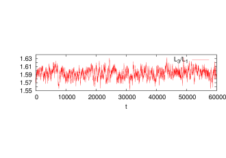
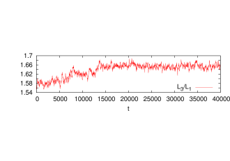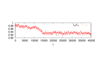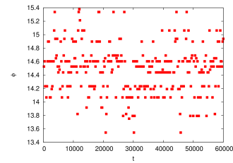
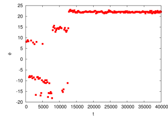
Since the new lattice structures break the symmetry between the $x$,$y$ directions and the $z$ direction, it is natural to expect them to be unstable when we let the system change its size in the three directions independently. We thus perform isobaric runs for systems of size $L_{1}\times L_{2}\times L_{3}$, updating independently $L_{1}$, $L_{2}$, and $L_{3}$. We start the simulations from the final configurations obtained in the two runs with $r_{\rm start}=1.5$ and 1.75. In both cases, see Fig. 16, after some iterations the symmetry under the exchange of $L_{1}$ and $L_{2}$ is broken and we obtain a body-centered lattice with unit cell given by

$${\bm{v}}_{1} = (a,0,0)$$

$${\bm{v}}_{2} = (b\tan\phi,b,0)$$

$${\bm{v}}_{3} = (0,0,c).$$ (50)

The angle $\phi$ is again obtained by performing a minimization procedure. The results are reported in Fig. 17. For the run with $r_{\rm start}=1.75$ we find $b/a\approx 0.97$, $c/a\approx 1.59$, and $\phi\approx 14^{\circ}$, while for the $r_{\rm start}=1.5$ we obtain $b/a\approx 0.93$, $c/a\approx 1.66$, and $\phi\approx 22^{\circ}$.

Figure 18: Plot of $N_{ms}(\epsilon)$ and of $N_{mf}(\epsilon)$, $\epsilon=0.2$, as a function of the number $t$ of iterations. Here $\widetilde{P}=10.0$. The starting configuration is a mixed solid-fluid system (1296 molecules) in which the solid is a tetragonal structure with $n=6$, $m=9$, and $c/a=1.5$.

Figure 19: Top panel: estimates of the ratio $L_{3}/(2L_{1})$ as a function of the number $t$ of iterations for the run starting from a mixed (fluid-solid) configuration with $n=m=6$ (864 molecules), $c/a=1$ (the solid is a bcc lattice), and $\Phi_{p}=0.9$. In the run we fix $\widetilde{P}=24$ and keep $L_{1}=L_{2}$. Middle and bottom panel: estimates of the ratios $L_{3}/(2L_{1})$ and $L_{2}/L_{1}$; the run starts from the final configuration obtained in the run considered in the top panel, but now $L_{1}$, $L_{2}$, and $L_{3}$ are updated independently. We always set $\widetilde{P}=24$.

Figure 20: Estimates of the ratios $L_{3}/(2L_{1})$ (top) and $L_{2}/L_{1}$ (bottom) as a function of the number $t$ of iterations. The simulation starts from a lattice configuration with 1024 molecules (8 unit cells in each lattice direction). The initial lattice is body-centered orthorombic with unit cell dimensions $a,b,c$. We fix $L_{2}/L_{1}=b/a=0.9$, $L_{3}/L_{1}=c/a=1.5$ and choose $a$ so that $\Phi_{p}=0.9$. In the run we set $\widetilde{P}=24$ and update $L_{1}$, $L_{2}$, and $L_{3}$ independently.

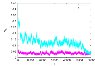
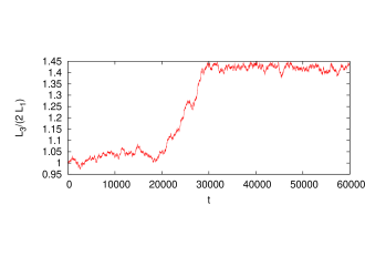
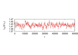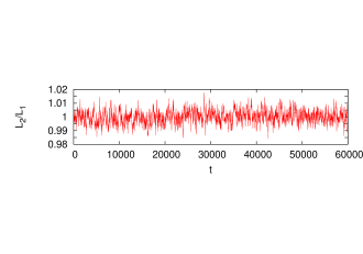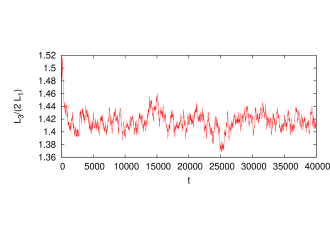
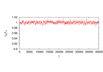We also perform simulations at $\widetilde{P}=10$ using mixed solid-fluid configurations, taking $c/a=1.5$ for the starting configuration. In this case, we find that the system melts, indicating that the tetragonal phase is less stable than the fluid, see Fig. 18. This confirms that the stable phase at the transition is the bcc lattice structure. However, by increasing the density, the relative stability of the different crystal structures can only be ascertained by performing a detailed free-energy calculation.

Simulations at $\widetilde{P}=24$ (the equilibrium packing fraction is $\Phi_{p}\approx 0.9$) indicate that asymmetric crystal structures become the stable ones as $\Phi_{p}$ increases. We have indeed performed a simulation for such value of $\widetilde{P}$, starting from a mixed system containing a bcc lattice with $n=m=6$ and a disordered configuration (the total number of particles is 864). We perform independent updates of $L_{3}$ and of $L_{1}$, keeping $L_{2}=L_{1}$. At the beginning $L_{3}/(2L_{1})=c/a$ is 1. In the simulation the disordered part of the system freezes, but at the same time $L_{3}/(2L_{1})$, which provides an estimate of $c/a$, changes, becoming approximately 1.4 at the end of the simulation, see Fig. 19. We have also analyzed in detail the configurations, looking for lattice structures generated by the vectors (48) and (49). We find $\phi\approx 0$, i.e., the stable lattice is centered tetragonal. Starting from the final configuration obtained in this run, we have performed a second simulation at $\widetilde{P}=24$, in which $L_{1}$, $L_{2}$, and $L_{3}$ are allowed to change independently. We find $L_{2}/L_{1}\approx 1$, see the two lower panels in Fig. 19, confirming the (meta)stability of the tetragonal structure. As a final check we have performed a new run with 1024 particles. We start from a body-centered orthorombic lattice with 8 unit cells in each direction and $L_{2}/L_{1}=b/a=0.9$, $L_{3}/L_{1}=c/a=1.5$ ($a,b,c$ give the size of the unit cell). The ratio $L_{2}/L_{1}$ as a function of the number of iterations is shown in Fig. 20. After a few iterations, we have again $L_{2}/L_{1}\approx 1$, indicating the stability of the tetragonal structure with respect to orthorombic deformations.

In conclusion, for the SB model, we estimate the pressure $P_{fs}$ at the low-density fluid-solid transition as

$$\widetilde{P}_{fs}=9.2(8).$$ (51)

If $\Phi_{p,f}$ and $\Phi_{p,s}$ are the boundaries of the fluid and solid phases, respectively, we obtain

$$0.60\mathrel{\hbox to0.0pt{\lower 3.0pt\hbox{$\mathchar 536\relax$}\hss}\raise 2.0pt\hbox{$\mathchar 316\relax$}}\Phi_{p,f}<\Phi_{p,s}\mathrel{\hbox to0.0pt{\lower 3.0pt\hbox{$\mathchar 536\relax$}\hss}\raise 2.0pt\hbox{$\mathchar 316\relax$}}0.64.$$ (52)

At the transition the bcc lattice is the stable crystal structure. The size $a$ of the corresponding unit cell is $a=2.38\hat{R}_{g}$, while the distance between the two closest lattice points is $a\sqrt{3}/2\approx 2.06\hat{R}_{g}$. As $\widetilde{P}$ and $\Phi_{p}$ increase, the bcc lattice becomes unstable. For $\widetilde{P}=24$ ($\Phi_{p}=0.9$) the stable lattice structure is apparently centered tetragonal.

Figure 21: Plot of the maximum $S_{\rm max}$ of the structure factor for the SB model in the CM representation, as a function of $\Phi_{p}$. It has been obtained by using the integral-equation method with Rogers-Young closure. The dotted-dashed line at $S_{\rm max}=2.85$ corresponds to the Hansen-Verlet criterion for the stability of the solid phase.

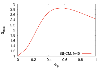
In Ref. MP-13-suppl, we used integral equation methods to estimate the location of the fluid-solid transition. In particular, we used the Hansen-Verlet criterion:HV-69-suppl ; HS-73-suppl the phase transition occurs when the maximum $S_{\rm max}$ of $S(q)$ exceeds 2.85. Unfortunately, the pair potential used there was not accurate, and therefore that result largely overestimates the correct pressure and density. Here, we have repeated the same calculation, using our estimate of the pair potential. The maximum of the structure factor $S_{\rm max}$ is reported in Fig. 21. It shows a nonmonotonic behavior with a maximum for $\Phi_{p}\approx 0.58$, where it takes the value 2.86, slightly larger than the Hansen-Verlet value of 2.85. If we were using the Hansen-Verlet criterion, we would estimate $\Phi_{p,f}\approx 0.54$, which is not far from the correct estimate obtained numerically.

We have also collected some data to estimate the high-density solid-fluid transition. For this purpose we have performed isobaric simulations with $\widetilde{P}=70,$ 100, 110, and 120, starting from mixed solid-fluid systems. The starting configuration is a centered tetragonal lattice with $m=n=6$, $c/a=1.5$, so that the total (solid and fluid) number of particles is 864. To verify the stability of the tetragonal structure with respect to orthorombic deformations we update $L_{1}$, $L_{2}$, and $L_{3}$ independently. For $\widetilde{P}=70$ the system freezes. At the end of the simulation, the lattice has a centered tetragonal structure with $c/a\approx 1.41$ (the same value found for $\widetilde{P}=24$) and $\Phi_{p}\approx 1.24$. For $\widetilde{P}=100$ and 110, the system is apparently unable to reach equilibrium. After approximately $10^{5}$ iterations, the system settles in an arrested state and particles no longer diffuse. The presence of arrested states was already noted FSTZLVWDL-03-suppl in SB models with phenomenological potentials, using a more realistic dynamics (here we use a Metropolis dynamics with local random displacements of the particles). Our results show that arrested states are a generic property of the SB models, which is not very dependent on the interaction potentials (the potentials we use are quite different from those used in Ref. FSTZLVWDL-03-suppl, , see Ref. MP-13-suppl, ) and on the dynamics. A visual inspection of the arrested configuration obtained in the run with $\widetilde{P}=100$ shows the molecules belonging to the fluid half-system have been able to partially order. Thus, we expect the stable phase for $\widetilde{P}=100$ to be solid. To identify the equilibrium value of $\Phi_{p}$ for $\widetilde{P}=100$, we perform a simulation in which we start from a solid centered tetragonal lattice with $n=m=8$ (1024 particles), $b/a=1$, $c/a=1.5$, $\Phi_{p}=1.4$. We find at the end $b/a\approx 1$, $c/a\approx 1.41$, and $\Phi_{p}\approx 1.27$. For $\widetilde{P}=110$, there is no indication of partial order. The arrested configuration consists in a perfectly ordered crystal coexisting with a fully disorderd half system. Finally, for $\widetilde{P}=120$, the solid part of the system melts in a few thousand iterations. The corresponding volume fraction is $\Phi_{p}\approx 1.66$. Therefore, the transition occurs for

$$\widetilde{P}_{sf}=110(10),$$ (53)

while the coexistence interval $[\Phi_{ps},\Phi_{pf}]$ satisfies $1.27\mathrel{\hbox to0.0pt{\lower 3.0pt\hbox{$\mathchar 536\relax$}\hss}\raise 2.0pt\hbox{$\mathchar 316\relax$}}\Phi_{ps}<\Phi_{pf}\mathrel{\hbox to0.0pt{\lower 3.0pt\hbox{$\mathchar 536\relax$}\hss}\raise 2.0pt\hbox{$\mathchar 316\relax$}}1.66$. At the transition, a centered tetragonal crystal with $c/a\approx 1.4$ is the stable solid structure.

B.6.3 The multi-blob model

Figure 22: Plot of $N_{ms}(\epsilon)$ and of $N_{mf}(\epsilon)$ as a function of the number $t$ of iterations. Top: $\widetilde{P}=6.6$; middle: $\widetilde{P}=5.0$; bottom: $\widetilde{P}=3.38$. Here $\epsilon=0.2$. Simulations with $500$ molecules and, for $\widetilde{P}=6.6$, also with 1152 molecules. For $\widetilde{P}=6.6$ and 5.0, the solid is stable; for $\widetilde{P}=3.38$ the stable phase is fluid.

Figure 23: Top: plot of $\phi$ (in degrees) as a function of the number $t$ of iterations (we estimate $\phi$ every 200 iterations): red points correspond to systems with unit cell given in Eq. (48), green points to systems with unit cell given in Eq. (49). Bottom: plot of $L_{3}/(2L_{1})=c/a$, as a function of $t$. Results for a system of 500 molecules and $\widetilde{P}=6.6$. We start from a mixed configuration with $c/a=1.5$ and $n=m=5$.

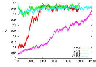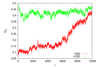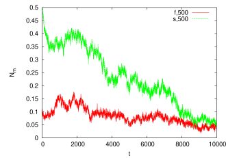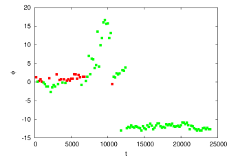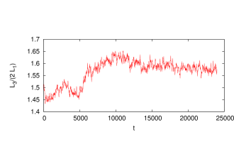The analysis presented in the SB case has been repeated for the MB model. Short runs on very small bcc systems with 128 molecules give indications that the solid phase might be stable for $\Phi_{p}\mathrel{\hbox to0.0pt{\lower 3.0pt\hbox{$\mathchar 536\relax$}\hss}\raise 2.0pt\hbox{$\mathchar 318\relax$}}0.5$. For this reason, we have performed simulations at $\widetilde{P}=10.9,6.6,3.38$, which are the values of the pressure obtained in canonical simulations starting from disordered configurations with $\Phi_{p}=0.6,0.5,$ and 0.4, respectively. For each packing fraction we generated mixed configurations with $c=a$ and $n=m=5$ (the total number of molecules is 500). They were used as starting configurations for isobaric runs in which $L_{1}$ and $L_{2}$ were kept equal. We find that the bcc phase is stable for $\widetilde{P}=10.9$ and 6.6, while for $\widetilde{P}=3.38$ the solid part of the system melts. This is evident from Fig. 22, where we report $N_{mf}(\epsilon)$ and $N_{ms}(\epsilon)$ for $\epsilon=0.2$. The results obtained using 500 molecules are confirmed by simulations with larger systems. In particular, we considered a starting mixed configuration with $n=6$ and $m=8$ (1152 molecules) at $\widetilde{P}=6.6$. Again, we observe that the bcc phase is stable, see Fig. 22. The densities obtained in the isobaric simulations for the solid phase do not differ significantly from those obtained in simulations in the (metastable) fluid phase (in these simulations we start from a disordered distribution of the molecules). For instance, for $\widetilde{P}=6.6$ we find $\Phi_{p}=0.5068(1)$ for the solid phase and $\Phi_{p}=0.5055(1)$ for the metastable fluid phase.

To improve the estimates of the transition pressure, we perform a simulation for $\widetilde{P}=5$. We find that the bcc lattice is the stable phase, see Fig. 22, and that the corresponding packing fraction is $\Phi_{p}=0.46$. We thus predict a fluid-solid transition for

$$\widetilde{P}_{fs}=4.2(8).$$ (54)

If $\Phi_{p,f}$ and $\Phi_{p,s}$ are the boundaries of the fluid and solid phases, respectively, we obtain

$$0.40\mathrel{\hbox to0.0pt{\lower 3.0pt\hbox{$\mathchar 536\relax$}\hss}\raise 2.0pt\hbox{$\mathchar 316\relax$}}\Phi_{p,f}<\Phi_{p,s}\mathrel{\hbox to0.0pt{\lower 3.0pt\hbox{$\mathchar 536\relax$}\hss}\raise 2.0pt\hbox{$\mathchar 316\relax$}}0.46.$$ (55)

Note that, for $\Phi_{p}\approx 0.43$, the size $a$ of the unit cell is $a=2.69\hat{R}_{g}$ and that the distance between the two closest lattice points is $a\sqrt{3}/2\approx 2.33\hat{R}_{g}$.

In the MB case, we have not performed a detailed analysis of other possible asymmetric lattice structures. We have only performed a single isobaric run at $\widetilde{P}=6.6$, starting with a mixed system with $c/a=1.5$ and $n=m=5$, and keeping $L_{1}=L_{2}$ in the simulation. After 12000 iterations, the disordered part of the system is completely frozen. The resulting lattice structure has $c/a\approx 1.6$ and is monoclinic with $\phi\approx 12$-$13^{\circ}$, see Fig. 23. Note that this result is completely analogous to what has been observed in the SB simulations (although at a different value of the pressure). Therefore, we conclude that the existence of these (meta)stable structures is not due the coarse-graining procedure, but that it is a property of the underlying star-polymer system.

Figure 24: Plot of $N_{ms}(\epsilon)$ and of $N_{mf}(\epsilon)$ as a function of the number $t$ of iterations. Top: $\widetilde{P}=70$ and starting configuration with $c/a=1$; middle: $\widetilde{P}=70$ and starting configuration with $c/a=1.5$; bottom: $\widetilde{P}=55$ and starting configuration with $c/a=1$. Here $\epsilon=0.2$. Simulations with $500$ molecules. For $\widetilde{P}=55$, the solid is stable; for $\widetilde{P}=70$ the stable phase is fluid.

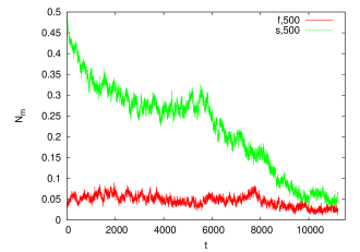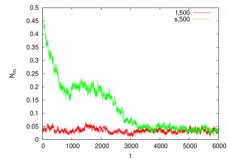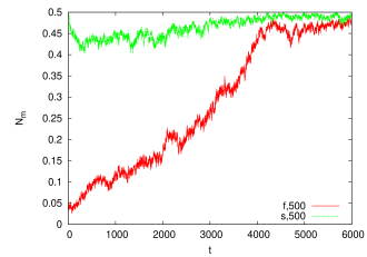Finally, we determined the location of the high-density solid-fluid transition. We performed simulations for $\widetilde{P}=24,55,$ 70, and 85, starting from mixed solid-fluid configurations with $m=n=5$ (500 particles) and $c/a=1$ (bcc lattice). For $\widetilde{P}=24$ (corresponding to $\Phi_{p}\approx 0.8$) and $\widetilde{P}=55$ (correspondingly $\Phi_{p}\approx 1.13$) the system freezes, while for $\widetilde{P}=70,85$, the solid part of the system melts and $\Phi_{p}\approx 1.26,1.38$, respectively, at the end of the simulation; see Fig. 24. Since it is possible that the stable phase is not cubic symmetric—it might be tetragonal, orthorombic, or monoclinic—we also performed simulations at $\widetilde{P}=70,85$, starting from mixed fluid-solid configurations with $c/a=1.5$ and $m=n=5$. In both cases, the crystal melts, confirming that the stable phase is fluid for $\widetilde{P}\mathrel{\hbox to0.0pt{\lower 3.0pt\hbox{$\mathchar 536\relax$}\hss}\raise 2.0pt\hbox{$\mathchar 318\relax$}}70$. Therefore, the solid-fluid transition occurs at

$$\widetilde{P}=62(8),$$ (56)

while the coexistence interval $[\Phi_{ps},\Phi_{pf}]$ satisfies $1.13\mathrel{\hbox to0.0pt{\lower 3.0pt\hbox{$\mathchar 536\relax$}\hss}\raise 2.0pt\hbox{$\mathchar 316\relax$}}\Phi_{ps}<\Phi_{pf}\mathrel{\hbox to0.0pt{\lower 3.0pt\hbox{$\mathchar 536\relax$}\hss}\raise 2.0pt\hbox{$\mathchar 316\relax$}}1.26$. Note that we have found no evidence of structural arrest in the multiblob case.

B.7 Numerical results

Table 5: Estimates of the compressibility factor $Z$ for $f=6$ and different values of $\Phi_{p}$. We report single-blob results in two different representations (SB-MP and SB-CM), multiblob results (MB), and estimates obtained by using the Padé extrapolation discussed in the paper (PADE).

	$\Phi_{p}=0.15$	$\Phi_{p}=0.25$	$\Phi_{p}=0.50$	$\Phi_{p}=0.75$	$\Phi_{p}=1$	$\Phi_{p}=2$
SB-MP	1.623	2.130	3.563	5.094	6.656	12.981
SB-CM	1.620	2.146	3.719	5.472	7.285	14.626
MB	1.638	2.182	3.927	5.919	8.132	17.782
PADE	1.618	2.141	3.776	5.797	8.132	19.74

Table 6: Estimates of the compressibility factor $Z$ for $f=12$ and different values of $\Phi_{p}$. We report single-blob results in two different representations (SB-MP and SB-CM), multiblob results (MB), and estimates obtained by using the Padé extrapolation discussed in the paper (PADE).

$\Phi_{p}$	$0.15$	$0.25$	$0.50$	$0.75$	$1$	$2$
SB-MP	2.255	3.532	7.587	11.998	16.440	34.116
SB-CM	2.258	3.601	8.196	13.490	18.920	40.450
MB	2.106	3.385	7.983	13.981	21.295	49.640
PADE	2.215	3.431	7.771	13.725	21.295	60.051

Table 7: Estimates of the compressibility factor $Z$ for $f=40$ and different values of $\Phi_{p}$. We report single-blob results in the center-of-mass representation (SB-CM)s and multiblob results (MB). All results refer to the fluid phase, which is metastable for $\Phi_{p}\mathrel{\hbox to0.0pt{\lower 3.0pt\hbox{$\mathchar 536\relax$}\hss}\raise 2.0pt\hbox{$\mathchar 318\relax$}}0.4$ (multiblob model) and for $\Phi_{p}\mathrel{\hbox to0.0pt{\lower 3.0pt\hbox{$\mathchar 536\relax$}\hss}\raise 2.0pt\hbox{$\mathchar 318\relax$}}0.6$ (single blob model).

$\Phi_{p}$	$0.15$	$0.25$	$0.50$	$0.75$	$0.90$
SB-CM	4.752	11.781	43.760	80.430	101.667
MB	4.785	12.552	54.977	112.576	147.169

Table 8: Estimates of the ratio $R_{g,b}(\Phi_{p})/\hat{R}_{g,b}$ for different values of $\Phi_{p}$ and $f$. For $f=40$, the results for $\Phi_{p}=0.50$ and 0.75 are obtained in the metastable fluid phase.

$f\backslash\Phi_{p}$	$0.15$	$0.25$	$0.50$	$0.75$	$1$	$2$
$6$	0.989	0.982	0.961	0.941	0.924	0.883
$12$	0.992	0.984	0.954	0.924	0.894	0.820
$40$	0.995	0.985	0.936	0.888	—	—

References

- (1) G. S. Grest, L. J. Fetters, J. S. Huang, and D. Richter, Star polymers: Experiment, theory, and simulation, Adv. Chem. Phys. 94, edited by I. Prigogine and S. A. Rice (Wiley, NY, 1996) pp. 67-163.
- (2) D. Vlassopoulos, G. Fytas, T. Pakula, and J. Roovers, Multiarm star polymers dynamics, J. Phys.: Condens. Matter 13, R855 (2001).
- (3) M. Daoud and J. P. Cotton, Star shaped polymers: a model for the conformation and its concentration dependence, J. Phys. (Paris) 43, 531 (1982).
- (4) T. M. Birshtein and E. B. Zhulina, Conformations of star-branched macromolecules, Polymer 25, 1453 (1984).
- (5) G. S. Grest, Structure of many-arm star polymers in solvents of varying quality: A molecular dynamics study, Macromolecules 27, 3493 (1994).
- (6) H.-P. Hsu, W. Nadler, and P. Grassberger, Scaling of star polymers with 1-80 arms, Macromolecules 37, 4658 (2004).
- (7) H.-P. Hsu and P. Grassberger, Effective interactions between star polymers, Europhys. Lett. 66, 874 (2004).
- (8) S. Huissmann, R. Blaak, and C. N. Likos, Star polymers in solvents of varying quality, Macromolecules 42, 2806 (2009).
- (9) F. Randisi and A. Pelissetto, High-functionality star-branched macromolecules: Polymer size and virial coefficients, J. Chem. Phys 139, 154902 (2013).
- (10) T. A. Witten and P. A. Pincus, Colloid stabilization by long grafted polymers, Macromolecules 19, 2509 (1986).
- (11) T. A. Witten, P. A. Pincus, and M. E. Cates, Macrocrystal ordering in star polymer solutions, Europhys. Lett. 2, 137 (1986).
- (12) C. N. Likos, H. Löwen, M. Watzlawek, B. Abbas, O. Jucknischke, J. Allgaier, and D. Richter, Star polymers viewed as ultrasoft colloidal particles, Phys. Rev. Lett. 80, 4450 (1998).
- (13) M. Watzlawek, H. Löwen, and C. N. Likos, The anomalous structure factor of dense star polymer solutions, J. Phys.: Condens. Matter 10, 8189 (1998).
- (14) M. Watzlawek, C. N. Likos, and H. Löwen, Phase diagram of star polymer solutions, Phys. Rev. Lett. 82, 5289 (1999).
- (15) M. Laurati, J. Stellbrink, R. Lund, L. Willner, D. Richter, and E. Zaccarelli, Starlike micelles with starlike interactions: A quantitative evaluation of structure factors and phase diagram, Phys. Rev. Lett. 94, 195504 (2005).
- (16) R. Menichetti and A. Pelissetto, Comparing different coarse-grained potentials for star polymers, J. Chem. Phys. 138, 124902 (2013).
- (17) F. Müller-Plathe, Coarse-graining in polymer simulation: From the atomistic to the mesoscopic scale and back, Chem. Phys. Chem. 3, 754 (2002).
- (18) G. A. Voth (Editor), Coarse-Graining of Condensed Phases and Biomolecular Systems (CRC Press, Boca Raton, 2009).
- (19) R. Faller (Editor), Coarse-grained modeling of soft condensed matter, Phys. Chem. Chem. Phys. 11, 1867 (2009).
- (20) M. Wilson (Editor), Themed issue: modelling of soft matter, Soft Matter 5, 4355 (2009).
- (21) C. Peter and K. Kremer, Multiscale simulation of soft matter systems — from the atomistic to the coarse-grained level and back, Soft Matter 5, 4357 (2009).
- (22) J. F. Rudzinski and W. G. Noid, Coarse-graining entropy, forces, and structures, J. Chem. Phys. 135, 214101 (2011).
- (23) W. G. Noid, Perspective: Coarse-grained models for biomolecular systems, J. Chem. Phys. 139, 090901 (2013).
- (24) A. Gooneie, S. Schuschnigg, and C. Holzer, A review of multiscale computational methods in polymeric materials, Polymers 9, 16 (2017).
- (25) A. A. Louis, P. G. Bolhuis, J. P. Hansen, and E. J. Meijer, Can polymer coils be modeled as “soft colloids”? Phys. Rev. Lett. 85, 2522 (2000).
- (26) C. N. Likos, Effective interactions in soft condensed matter physics, Phys. Rep. 348, 267 (2001); Soft matter with soft particles, Soft Matter 2, 478 (2006).
- (27) P. G. Bolhuis, A. A. Louis, J. P. Hansen, and E. J. Meijer, Accurate effective pair potentials for polymer solutions, J. Chem. Phys. 114, 4296 (2001).
- (28) C. Pierleoni, B. Capone, and J. P. Hansen, A soft effective segment representation of semidilute polymer solutions, J. Chem. Phys. 127, 171102 (2007).
- (29) A. Pelissetto, Coarse-grained models for semi-dilute polymer solutions under good-solvent conditions, J. Phys.: Condens. Matt. 21, 115108 (2009).
- (30) G. D’Adamo, A. Pelissetto, and C. Pierleoni, Coarse-graining strategies for polymer solutions, Soft Matter 8, 5151 (2012).
- (31) G. D’Adamo, R. Menichetti, A. Pelissetto, and C. Pierleoni, Coarse-Graining Polymer Solutions: A critical appraisal of single- and multi-site models, Eur. Phys. J. Spec. Topics 224, 2239 (2015).
- (32) A. Jusufi, J. Dzubiella, C.N. Likos, C. von Ferber, and H. Löwen, Effective interactions between star polymers and colloidal particles, J. Phys.: Condens. Matter 13, 6177 (2001).
- (33) G. D’Adamo, A. Pelissetto, and C. Pierleoni, Consistent and transferable coarse-grained model for semidilute polymer solutions in good solvent, J. Chem. Phys. 137, 024901 (2012).
- (34) C. Domb and G. S. Joyce, Cluster expansion for a polymer chain, J. Phys. C 5, 956-976 (1972).
- (35) G. D’Adamo and A. Pelissetto, Improved model for mixtures of polymers and hard spheres, J. Phys. A: Math. Theor. 49, 504006 (2016).
- (36) S. Caracciolo, B. M. Mognetti, and A. Pelissetto, Virial coefficients and osmotic pressure in polymer solutions in good-solvent conditions, J. Chem. Phys. 125, 094903 (2006).
- (37) Much longer arms would be needed if one were using lattice self-avoiding walks (see Ref. RP-13, ). The Kremer-Grest model, which is often used to simulate star polymers, would behave even worse, as finite-length corrections in the latter model are roughly twice as large as those for lattice self-avoiding walks; see G. D’Adamo and A. Pelissetto, Thick self-avoiding chains: thickness crossover and optimal good-solvent behavior, submitted.
- (38) W. Schommers, Pair potentials in disordered many-particle systems: A study for liquid gallium, Phys. Rev. A 28, 3599 (1983).
- (39) D. Reith, M. Pütz, and F. Müller-Plathe, Deriving effective mesoscale potentials from atomistic simulations, J. Comp. Chem. 24, 1624 (2003).
- (40) S. Caracciolo, B. M. Mognetti, and A. Pelissetto, Third virial coefficient for four-arm and six-arm star polymers, Macromol. Theory Simul. 17, 67 (2008).
- (41) J. P. Hansen and I. McDonald, Theory of Simple Liquids with Applications to Soft Matter, 4th ed. (Academic Press, Amsterdam, 2013).
- (42) F. J. Rogers and D. A. Young, New, thermodynamically consistent, integral equation for simple fluids, Phys. Rev. A 30, 999 (1984).
- (43) G. Ciccotti and J. P. Ryckaert, Molecular dynamics simulation of rigid molecules, Comp. Phys. Rep. 4, 346 (1986).
- (44) R. L. C. Akkermans and G. Ciccotti, On the equivalence of atomic and molecular pressure, J. Phys. Chem. B 108, 6866 (2004).
- (45) P. G. de Gennes, Scaling Concepts in Polymer Physics (Cornell University Press, Ithaca, NY, 1979).
- (46) K. F. Freed, Renormalization Group Theory of Macromolecules (Wiley, New York, 1987).
- (47) J. des Cloizeaux and G. Jannink, Polymers in Solution: Their Modelling and Structure (Clarendon, Oxford, 1990).
- (48) A. Pelissetto, Osmotic pressure and polymer size in semidilute polymer solutions under good-solvent conditions, J. Chem. Phys. 129, 044901 (2008).
- (49) B. J. Cherayil, M. G. Bawendi, A. Miyake, and K. F. Freed, Osmotic pressure of star and ring polymers in semidilute solutions, Macromolecules 19, 2770 (1986).
- (50) J. F. Douglas, J. Roovers, and K. F. Freed, Characterization of branching architecture through ”universal” ratios of polymer solution properties, Macromolecules 23, 4168 (1990).
- (51) G. Merkle, W. Burchard, P. Lutz, K. F. Freed, and J. Gao, Osmotic Pressure of Linear, Star, and Ring Polymers in Semidilute Solution. A Comparison between Experiment and Theory, Macromolecules 26, 2736 (1993).
- (52) A. J. C. Ladd and L. V. Woodcock, Triple-point coexistence properties of the Lennard-Jones system, Chem. Phys. Lett. 51, 155(1977); Interfacial and coexistence properties of the Lennard-Jones system at the triple point, Mol. Phys. 36, 611(1978).
- (53) J. N. Cape and L. V. Woodcock, Molecular dynamics calculation of phase coexistence properties: The soft-sphere melting transition, Chem. Phys. Lett. 59, 271 (1977).
- (54) E. G. Noya, C. Vega, and E. de Miguel, Determination of the melting point of hard spheres from direct coexistence simulation methods, J. Chem. Phys. 128, 154507 (2008).
- (55) J. R. Espinosa, E. Sanz, C. Valeriani, and C. Vega, On fluid-solid direct coexistence simulations: The pseudo-hard sphere model, J. Chem. Phys. 139, 144502 (2013)
- (56) A. J. Archer, C. N. Likos, and R. Evans, Binary star-polymer solutions: bulk and interfacial properties, J. Phys.: Condens. Matter 14, 12031 (2002).
- (57) J. Dzubiella, C. N. Likos, and H. Löwen, Phase behavior and structure of star-polymer–-colloid mixtures, J. Chem. Phys. 116, 9518 (2002).
- (58) M. Camargo and C. N. Likos, Unusual features of depletion interactions in soft polymer-based colloids mixed with linear homopolymers, Phys. Rev. Lett. 104, 078301 (2010).
- (59) B. Lonetti, M. Camargo, J. Stellbrink, C. N. Likos, E. Zaccarelli, L. Willner, P. Lindner, and D. Richter, Ultrasoft colloid-polymer mixtures: structure and phase diagram, Phys. Rev. Lett. 106, 228301 (2011).
- (60) E. Locatelli, B. Capone, and C. N. Likos, Multiblob coarse-graining for mixtures of long polymers and soft colloids, J. Chem. Phys. 145, 174901 (2016).
- (61) T. Vettorel, G. Besold, and K. Kremer, Fluctuating soft-sphere approach to coarse-graining of polymer models, Soft Matter 6, 2282 (2010).
- (62) G. D’Adamo, A. Pelissetto, and A. Pierleoni, Polymers as compressible soft spheres, J. Chem. Phys. 136, 224905 (2012).
- (63) R. L. C. Akkermans and W. J. Briels, A structure-based coarse-grained model for polymer melts, J. Chem. Phys. 114, 1020 (2001); Coarse-grained interactions in polymer melts: A variational approach, J. Chem. Phys. 115, 6210 (2001).
- (1) J. P. Hansen and I. McDonald, Theory of Simple Liquids with Applications to Soft Matter, 4th ed. (Academic Press, Amsterdam, 2013).
- (2) F. J. Rogers and D. A. Young, New, thermodynamically consistent, integral equation for simple fluids, Phys. Rev. A 30, 999 (1984).
- (3) C. N. Likos, H. Löwen, M. Watzlawek, B. Abbas, O. Jucknischke, J. Allgaier, and D. Richter, Star polymers viewed as ultrasoft colloidal particles, Phys. Rev. Lett. 80, 4450 (1998).
- (4) M. Watzlawek, C. N. Likos, and H. Löwen, Phase diagram of star polymer solutions, Phys. Rev. Lett. 82, 5289 (1999).
- (5) R. Menichetti and A. Pelissetto, Comparing different coarse-grained potentials for star polymers, J. Chem. Phys. 138, 124902 (2013).
- (6) B. J. Cherayil, M. G. Bawendi, A. Miyake, and K. F. Freed, Osmotic pressure of star and ring polymers in semidilute solutions, Macromolecules 19, 2770 (1986).
- (7) J. F. Douglas, J. Roovers, and K. F. Freed, Characterization of branching architecture through ”universal” ratios of polymer solution properties, Macromolecules 23, 4168 (1990).
- (8) G. Merkle, W. Burchard, P. Lutz, K. F. Freed, and J. Gao, Osmotic Pressure of Linear, Star, and Ring Polymers in Semidilute Solution. A Comparison between Experiment and Theory, Macromolecules 26, 2736 (1993).
- (9) C. Domb and G. S. Joyce, Cluster expansion for a polymer chain, J. Phys. C 5, 956 (1972).
- (10) H.-P. Hsu, W. Nadler, and P. Grassberger, Scaling of star polymers with 1-80 arms, Macromolecules 37, 4658 (2004); H.-P. Hsu and P. Grassberger, Effective interactions between star polymers, Europhys. Lett. 66, 874 (2004).
- (11) F. Randisi and A. Pelissetto, High-functionality star-branched macromolecules: Polymer size and virial coefficients, J. Chem. Phys 139, 154902 (2013).
- (12) N. Clisby, Accurate estimate of the critical exponent for self-avoiding walks via a fast implementation of the pivot algorithm, Phys. Rev. Lett. 104, 055702 (2010).
- (13) A. Aharony and G. Ahlers, Universal ratios among correction-to-scaling amplitudes and effective critical exponents, Phys. Rev. Lett. 44, 782 (1980).
- (14) P. Belohorec and and B. G. Nickel, Accurate universal and two-parameter model results from a monte-carlo renormalization group study, Guelph University report, 1997 (unpublished); P. Belohorec, Renormalization group calculation of the universal critical exponents of a polymer molecule, Guelph University Phd thesis, 1997 (available at www.collectionscanada.gc.ca/obj/s4/f2/dsk3/ftp04/nq24397.pdf).
- (15) S. Caracciolo, B. M. Mognetti, and A. Pelissetto, Virial coefficients and osmotic pressure in polymer solutions in good-solvent conditions, J. Chem. Phys. 125, 094903 (2006).
- (16) G. D’Adamo and A. Pelissetto, Improved model for mixtures of polymers and hard spheres, J. Phys. A 49, 504006 (2016).
- (17) N. Clisby, High resolution Monte Carlo study of the Domb-Joyce model, arXiv:1705.01249.
- (18) N. Madras and A. D. Sokal, The pivot algorithm: A highly efficient Monte Carlo method for the self-avoiding walk, J. Stat. Phys. 50, 109 (1988).
- (19) T. Kennedy, A faster implementation of the pivot algorithm for self-avoiding walks, J. Stat. Phys. 106, 407 (2002).
- (20) J. P. Hansen and L. Verlet, Phase transitions of the Lennard-Jones system, Phys. Rev. 184, 151 (1969).
- (21) J. P. Hansen and D. Schiff, Influence of interatomic repulsion on the structure of liquids at melting, Mol. Phys. 25, 1281 (1973).
- (22) G. Foffi, F. Sciortino, P. Tartaglia, E. Zaccarelli, F. Lo Verso, L. Reatto, K. A. Dawson, and C. N. Likos, Structural arrest in dense star-polymer solutions, Phys. Rev. Lett. 90, 238301 (2003).