Understanding solar cycle variability
Abstract
Version:
The level of solar magnetic activity, as exemplified by the number of sunspots and by energetic events in the corona, varies on a wide range of time scales. Most prominent is the 11-year solar cycle, which is significantly modulated on longer time scales. Drawing from dynamo theory together with empirical results of past solar activity and of similar phenomena on solar-like stars, we show that the variability of the solar cycle can be essentially understood in terms of a weakly nonlinear limit cycle affected by random noise. In contrast to ad-hoc ‘toy models’ for the solar cycle, this leads to a generic normal-form model, whose parameters are all constrained by observations. The model reproduces the characteristics of the variable solar activity on time scales between decades and millennia, including the occurrence and statistics of extended periods of very low activity (grand minima). Comparison with results obtained with a Babcock-Leighton-type dynamo model confirms the validity of the normal-mode approach.
1 Introduction
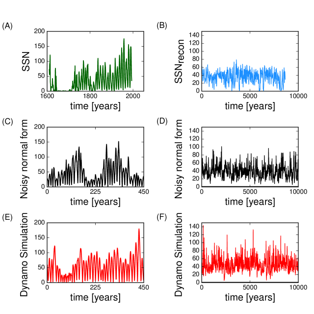
Apart from its 11-year (quasi)periodicity, the most striking property of the solar activity record is the marked variability of the cycle amplitudes (cf. top panels of Fig. 1), including extended intervals of very low or particularly high activity (grand minima and maxima, see Usoskin, 2017). Understanding the nature of the variability is a prerequisite for sensible attempts to predict future activity levels. Therefore, we need to clarify to what extent randomness, intrinsic periodicities apart from the 11-year cycle, and nonlinearities of the underlying dynamo process generating the solar magnetic field contribute to the observed long-term variability of solar activity.
There exists a rich literature describing attempts to understand the variability in the framework of hydromagnetic dynamo theory, a full review of which is beyond the scope of this paper (see, e.g., Tobias, 2002; Charbonneau, 2010, 2014). Such studies can be roughly divided into two approaches: (1) nonlinear dynamics and deterministic chaos, and (2) random fluctuations of dynamo excitation. The nonlinear dynamics approach typically considers the bifurcation structure of low-order dynamical systems (see reviews by Weiss, 1990; Tobias et al., 1995; Lopes et al., 2014), but models based on nonlinear PDEs have also been investigated frequently (e.g., Schmitt & Schuessler, 1989; Tobias, 1997; Bushby, 2006). Studies assuming random fluctuations reach from the minimalistic ‘model’ of Barnes et al. (1980) to detailed considerations of the mode structure of stochastically excited dynamos (Hoyng, 1993; Hoyng & van Geffen, 1993; Ossendrijver & Hoyng, 1996). Most of these studies adopt an -type dynamo approach with random fluctuations of the -effect thought to result from the non-stationary nature of solar convection (e.g. Choudhuri, 1992; Moss et al., 1992; Ossendrijver et al., 1996). There are also studies combining nonlinear dynamo models with random fluctuations, either in the framework of low-order dynamical systems (e.g. Mininni et al., 2001; Passos & Lopes, 2011) or assuming detailed dynamo models (e.g. Charbonneau & Dikpati, 2000; Mininni & Gómez, 2002; Moss et al., 2008; Lemerle & Charbonneau, 2017). Grand minima can also result from of ‘on-off intermittency’ due to the interaction of two spatially separated dynamos (Platt et al., 1993; Schmitt et al., 1996; Passos et al., 2014). Recently, Olemskoy et al. (2013) have estimated the fluctuating source term of a Babcock-Leighton-type dynamo considering the observed scatter of the tilt angles of sunspot groups. Assuming weakly supercritical dynamo excitation, the simulated long-term evolution of solar activity exhibits grand minima whose statistics are consistent with the actual solar record (see also Kitchatinov & Olemskoy, 2016). Global 3D-MHD simulations of convection and magnetic field in a rotating spherical shell typically show strong variability of dynamo-generated magnetic field and may also provide cyclic fields (e.g. Augustson et al., 2015; Passos & Charbonneau, 2014; Käpylä et al., 2016; Hotta et al., 2016; Fan & Fang, 2016). However such simulations remain far from the Sun in terms of various parameters, and so the variability seen in the simulations is not yet directly relatable to that of the Sun.
Although no definite quantitative model of the global dynamo exists so far, the basic ingredients are uncontroversial. The systematic properties of sunspot groups (Hale et al., 1919) indicate that they originate from a reservoir of organized East-West orientated (toroidal) field in the solar convection zone. This field is generated by winding up a poloidal field (such as a dipole field aligned with the rotation axis) by the differential rotation of the Sun, so that its axisymmetric component dominates. The poloidal field is (re)generated against the effect of Ohmic decay by the collective effect of loops formed from the toroidal field by convective flows and/or magnetic buoyancy. The loops become twisted owing to the Coriolis force and thus acquire a systematic meridional component (Parker, 1955; Babcock, 1961; Steenbeck & Krause, 1966). This interplay of toroidal and poloidal magnetic field leads to a 22-year magnetic cycle and an 11-year cycle of sunspot activity.
Here we consider these basic ingredients of solar dynamo theory together with solar and stellar observations to elucidate the nature of the variability of the solar cycle. We argue that the dynamo works near its excitation threshold (marginal state), so that a normal-form model representing the essence of the underlying dynamo process can be used. This model is generic in the sense that it is valid for any weakly nonlinear system in the vicinity of a supercritical Hopf bifurcation, independent of the nature of the nonlinearity. The very setup of the model and its parameters are all constrained by observations.
2 Generic normal-form model
Irrespective of the details of most models for the solar dynamo proposed so far, the corresponding systems of equations for the magnetic field components show qualitatively similar behaviour near the onset of dynamo action, which is governed by a control parameter (often called ‘dynamo number’) involving differential rotation, Coriolis effect, and magnetic diffusion. As long as the control parameter remains below a critical value, the stationary solution has zero magnetic field and the dynamo is not excited. When the critical value of the control parameter is exceeded, the system exhibits a periodic solution. This behaviour is generic for almost all models of the global solar dynamo (technically named dynamos). In the language of dynamical systems, the periodic solution emerges from a (supercritical) Hopf bifurcation: a fixed point becomes unstable and spawns a limit cycle (Guckenheimer & Holmes, 1983; Tobias et al., 1995).
The study of solar-like stars has revealed that the level of magnetic activity systematically declines with decreasing stellar rotation rate (e.g., Reiners, 2012; Reiners et al., 2014). In particular, the relatively slow rotation rate of the Sun appears to put it near to the threshold for which global dynamo action ceases (van Saders et al., 2016; Metcalfe et al., 2016). This allows us, irrespective of the nature of the nonlinearity that limits the amplitude of the cycle, to describe the solar dynamo generically by the normal form of a weakly nonlinear system near a Hopf bifurcation, which is independent of the nature of the nonlinearity (Arnol’d, 1972; Guckenheimer & Holmes, 1983), viz.
| (1) |
where is a complex variable. Its real and imaginary components are related to the toroidal and poloidal components of the magnetic field in a manner that depends on the kind of nonlinearity considered (e.g., back reaction on the differential rotation or quenching of the regeneration term for the poloidal field). We may therefore consider the real or the imaginary part of to represent the cyclically varying field magnitude. For simplicity, we take the activity level as quantified by the sunspot number, SSN, to be proportional to the absolute value of the field and write , thus scaling in units of the sunspot number. This quantity represents the 11-year sunspot cycle, in contrast to the 22-year magnetic cycle reflected in and .
The quantity in Eq. (1) is the linear growth rate of the cycle amplitude (related to the dynamo excitation, i.e., supercriticality of the dynamo number) and is the (magnetic) cycle frequency in the limit of zero amplitude. The parameters and generically represent the nonlinearity of the system. They determine the cycle amplitude, , and the nonlinear cycle frequency, .
In order to study the variability of the cycle amplitude, we need to account for the randomness inherent to the dynamo process. There is strong evidence that the dynamo is of Babcock-Leighton type (Wang & Sheeley, 2009; Muñoz-Jaramillo et al., 2013). This means that magnetic flux connected to the polar fields (axial dipole) is the relevant poloidal field for the generation of the toroidal field by differential rotation in the convection zone (Cameron & Schüssler, 2015). The polar fields result from the emergence of bipolar magnetic regions (sunspot groups) with a systematic average tilt relative to the solar East-West direction together with the subsequent transport of their magnetic flux across the surface by differential rotation, supergranulation, and meridional flow (Mackay & Yeates, 2012; Wang, 2016). Consequently, any scatter in the properties of the bipolar regions (e.g., emergence latitude, tilt angle) or in the flux transport process introduces a corresponding scatter in the resulting poloidal dipole field and, therefore, in the amplitude the subsequent cycle (Charbonneau & Dikpati, 2000; Wang & Sheeley, 2009; Jiang et al., 2014). Since Babcock-Leighton dynamos can be put into the general mathematical framework of -dynamos (Stix, 1974), we can describe this effect by random scatter in the term generating the poloidal field, which enters the normal form model in the form of multiplicative noise. Eq. (1) thus transforms into a stochastic differential equation, viz.
| (2) |
where we take to represent a complex Wiener process (random walk with uncorrelated, Gaussian distributed increments) with a variance of unity after 11 years. The real parameter then corresponds to the standard deviation of the cycle amplitudes due to the noise in the generation process.
Values for all five parameters entering Eq. (2) are constrained by empirical results. The linear growth rate, , can be estimated from the time scale for the recovery from a grand minimum of very low activity. The duration of the Maunder minimum of about 70 years implies a recovery time of the order of decades, so that we take year-1 as a reference value. The activity cycle appears to have persisted at low amplitude and with unchanged period during the Maunder minimum (Beer et al., 1998; Vaquero et al., 2015), so that we take the (magnetic) cycle frequency to be unaffected by the weak nonlinearity, year-1, and thus . In order to fix the parameter , we need to determine the (average) cycle amplitude, , in terms of the sunspot number. For a cycle of sinusoidal shape, the amplitude is given by times its mean level. Using the average of the Group Sunspot Numbers (Hoyt & Schatten, 1998) since 1700, the end of the Maunder minimum, we obtain a cycle amplitude of 64 and thus year-1.
The remaining parameter to be fixed is the noise level, , which we relate to the scatter of the tilt angles of bipolar magnetic regions. Surface flux transport simulations show that the observed Gaussian scatter of the tilt angles leads to a fluctuation level of 30%–40% of the polar dipole field (Jiang et al., 2014; Muñoz-Jaramillo et al., 2013). This implies a degree of fluctuations of the cycle amplitudes owing to the linear correlation between the polar field at the end of a cycle and the amplitude of the next cycle (Wang & Sheeley, 2009). This level is consistent with the value of about 35% for the scatter of the cycle amplitudes determined from the sunspot numbers observed since 1700 amounts and also with the scatter shown by the 10-year sampled sunspot numbers reconstructed from the cosmogenic isotopes (Usoskin et al., 2016). Since the limit cycle is an attractor, we have a slight damping of the random perturbations during a cycle, so that we have to use a somewhat higher value, , in order to compensate for this effect and reproduce the observed cycle-to-cycle fluctuation of 35%. The effect on the results of varying the parameters and is discussed further below.
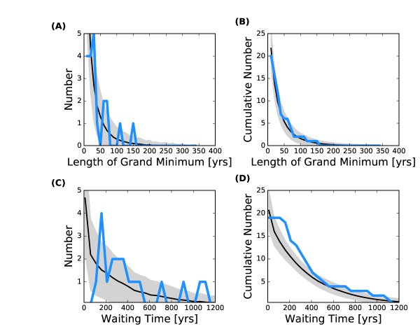
We used the Euler-Maruyama method (Kloeden & Platen, 1992) to perform Monte-Carlo simulations of Eq. (2) with the parameter values given above and a time step of one day. Random numbers were generated with the routine ‘random.normal’ from the Python package ‘numpy’ version 1.10.4. The convergence of the numerical result was checked against the analytic solution of the normal form without noise. Covering 10,000 years for each realization, we obtained the amplitude variability over a large range of time scales. Results for one such realization are illustrated in the middle panels of Fig. 1. Panel C covers a period of 450 years, exhibiting extended periods of very low activity (grand minima). Panel D shows the 10-year averages for the whole time interval of 10,000 years. The main features of the actual and the simulated time series are qualitatively similar: there is considerable variability of the cycle amplitudes with occasional grand minima (and maxima). For a more quantitative comparison, Fig. 2 gives the non-cumulative (left panels) and cumulative (right panels) distributions of the lengths of grand minima and of the waiting times between the end of one grand minimum and the start of the next from the simulations (black lines) in comparison to the empirical distributions (blue lines) derived from the cosmogenic isotope record (Usoskin et al., 2016). The model distributions are well approximated by exponentials, which would be expected for a Poisson process (see also Olemskoy et al., 2013). Overall, the distributions appear to be consistent with each other. Whether the empirical events in the tail of the waiting time distribution represent a significant deviation from an exponential distribution (cf. Moss et al., 2008) cannot be decided owing to the small number (20) of grand minima in the isotope record. Note that the normal-form model generically shows ongoing low-amplitude cycles during grand minima, such as indicated during the Maunder minimum (Beer et al., 1998; Vaquero et al., 2015).
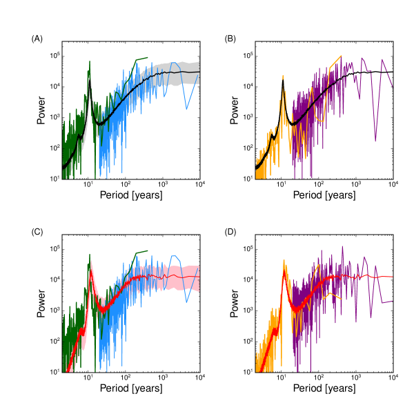
Further quantitative comparison between model and data is obtained by considering power spectra as shown in Fig. 3. Panel A corresponds to the historical sunspot record (yearly resolution, green line) and to the reconstruction based on cosmogenic isotopes (10-year resolution, blue line) in comparison to the median of 1000 realizations of 10,000 years each of the normal-form model (black line). The model results are consistent with the observed spectra, demonstrating that a weakly nonlinear limit cycle driven by random noise is sufficient to explain the observed variability of solar activity on a wide range of time scales. A single realization of the model is considered in panel B of Fig. 3, which shows spectra for 450 years with yearly resolution (orange line) and for 10,000 years with 10-year resolution (purple line). These spectra are qualitatively similar to the observed spectra shown in panel A, including some apparent (but spurious) long-term periodicities.
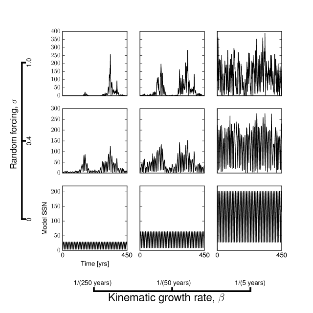
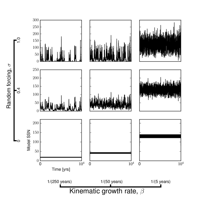
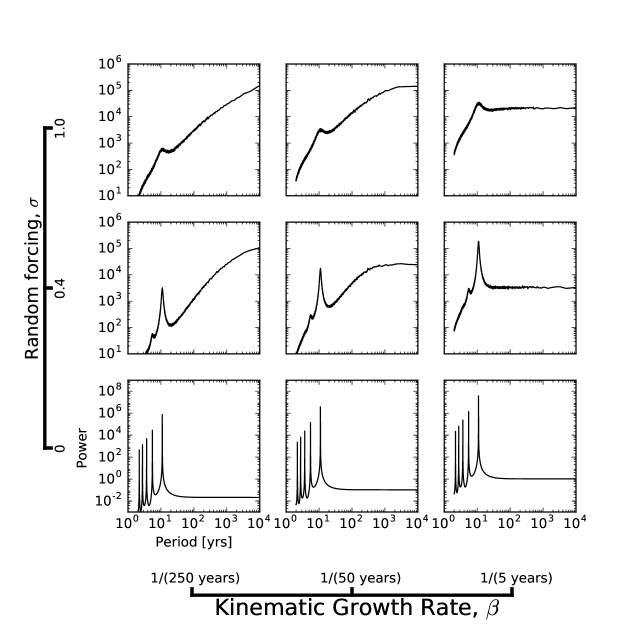
We also considered the effect of varying the parameters (linear growth rate, related to the supercriticality of the dynamo) and , the level of the random forcing. They represent two competing effects: the forcing tends to drive the solution away from the limit cycle while perturbations of the stable limit cycle decay with a timescale . Changing these parameters therefore varies the relative importance of the two effects. In addition to the reference value, year-1, suggested by the recovery of the Sun from the Maunder minimum, we considered values representing a much smaller growth rate, year-1, and a markedly higher growth rate, year-1. Likewise, we took values for the random forcing of (no perturbations) and (very strong perturbations), in addition to the reference value of indicated by the observed variability of the solar cycle maxima.
For the cases with year-1 and year-1 we performed 1000 simulations of 11,000 years length each. We excluded the first 1,000 years from each realization in order to stay clear of the transients related to the arbitrary initial conditions. For the very weakly excited cases with year-1, we run 1000 simulations of 21,000 years length each, excluding the first 11,000 years from the analysis. To illustrate the results, a stretch of 450 years of one arbitrarily chosen realization for each pair of parameters is shown in Fig. 4, while 10-year running averages covering 10,000 years are given in in Fig. 5. In the cases without random forcing (bottom rows of the figures), the solutions are rectified sine functions with amplitude . For the observationally well constrained reference value of the random forcing, , the cycles show variations in amplitude and phase (middle rows in Figs. 4 and 5). The value of determines the rate of occurrence and the lengths of grand minima: since the recovery time from perturbations is , low values of lead to long extended minima, while high values suppress their occurrence. In the case of very strong random forcing (top rows of Figs. 4 and 5), the perturbations lead to high cycle-to-cycle fluctuations and to very long grand minima for low . From these results, we would expect that very slowly rotating stars, which are even nearer to critical dynamo excitation, show very long quiescent phases, while stars with higher excitation (faster rotators) display very strong cycle-to-cycle fluctuations and, if at all, only rarely show short grand minima of activity.
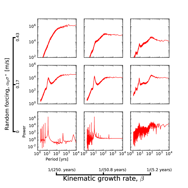
Fig. 3 shows median power spectra corresponding to 1000 realizations for each of the nine parameter combinations. The case without perturbations (bottom row) obviously shows the spectra of a rectified sine wave. For growing strength of the random forcing, the 11-year peak becomes less prominent and broader as the amplitude and phase fluctuations of the cycles grow stronger. For growing dynamo excitation (higher ), the long-period tail of the spectrum flattens as a result of the shortening and increasing suppression of the grand minima.
3 Babcock-Leighton-type dynamo model
To demonstrate that the normal-form approach actually fits in the context of a more detailed nonlinear dynamo model, we consider an updated version of the Babcock-Leighton dynamo (Babcock, 1961; Leighton, 1969; Wang et al., 1991), which reproduces key features of the solar cycle (Cameron & Schüssler, 2017). The model comprises the essential ingredients of a flux-transport dynamo (Charbonneau, 2010, 2014). It considers the axisymmetric part of the magnetic field and is based on the evolution equations for the azimuthal component of the vector potential (determining the poloidal field) at the solar surface,
| (3) |
and the radially integrated toroidal flux per radian,
| (4) |
both as functions of colatitude, , and time. Here, is the solar radius, the radial location of the bottom the solar convection zone. and are the radial and azimuthal components, respectively, of the magnetic field. Introducing fluctuations in the source term for the poloidal field, the evolution equations given in Cameron & Schüssler (2017) become stochastic differential equations, viz.
| (5) | |||||
and
| (6) | |||||
Here and are, respectively, the angular rotation rates at the solar surface and at the base of the near-surface shear layer, for which we take the same profiles as in Cameron & Schüssler (2017). kms-1 and are, respectively, the magnetic diffusivities at the solar surface and in the bulk of the convection zone. represents the poleward meridional flow at the surface, for which we use the profile given by Hathaway & Rightmire (2011, see their Eqs. 9–11). refers to the equatorward return flow affecting the toroidal field in the bulk of the convection zone; we take ms-1, which roughly corresponds to the speed of equatorward propagation of the activity belts. is the source of the poloidal field resulting from the emergence of bipolar magnetic regions, which we write as
| (7) |
where we have introduced a nonlinearity with parameter . The quantities , , and are the free parameters of the model.
The random forcing is considered as a two-dimensional Wiener process, , which depends on both latitude and time and has a variance of 1 radian-1 after 11 years. The strength of the forcing is determined by the parameter . Since the noise parameter, , in the normal-form model is independent of the growth rate (dynamo excitation), for consistency we take to represent a fixed noise level. In the computations, we used a second-order centered difference scheme for the spatial derivatives with 180 grid points in colatitude, and advanced the solution in time using the Euler-Maruyama method with a time step of 1 day. The numerical results for mildly supercritical, nonlinear dynamo action with this model ( kms-1, ms-1, Mx, and ms-1 where is the critical value of for the onset of dynamo action with the other parameters as stated), are shown in the bottom panels of Figs. 1 and 3. The measure of the activity shown here is the integrated subsurface toroidal field corresponding to the dipole mode of the dynamo , scaled to a similar level as the sunspot number. They are consistent with the results from observations and from the generic noisy normal-form model.
We also carried out a parameter study with this dynamo model. There is no simple relationship between the four free parameters of the Babcock-Leighton model (, , and ) and the four parameters of the normal-form model (, , and ). We have chosen parameters so that the solutions have a period of about 22 years (i.e. an 11-year activity cycle) and kinematic growth rates and levels of noise similar to those of the cases presented in the previous section for the normal-form model. This specifies three of the four degrees of freedom. The fourth constraint is equivalent to specifying the amplitude of the limit cycle. In this illustrative study we have kept Mx and expect solutions of this order of magnitude – the exact amplitude of the limit cycle will however also depend on the other parameters in a non-trivial way.
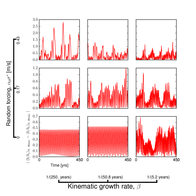
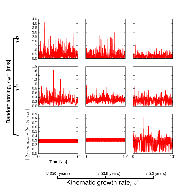
The results of the parameter study are illustrated in Figs.7–9, which show the corresponding quantities in the same format as in Figs. 4–6 for the normal-form model. For cases with a very low kinematic growth rate of 1/250 year-1 (left column of the figures) we took ms-1 and kms-1. For the cases with a growth rate of 1/50.8 year-1 (middle column) we chose ms-1 and kms-1. Finally, for the case with a high growth rate of 1/5.2 year-1 (right column) we used ms-1 and kms-1. For the purpose of a qualitative comparison, it is unnecessary to perform a tedious fine tuning of the parameters in order to exactly match the growth rates to those of the normal-form model. The cases without random forcing are shown in the bottom row of Figs. 7–9. The forcing for the cases given in the middle row reproduces the observed variability of the sunspot maxima since 1700 for the reference case (central panel of the figures). For the cases with very strong forcing (top row of the figures) we multiplied the reference value by the same factor 2.5 as in the case of the normal-form model. In all cases, we carried out 150 simulations covering a time of 11,000 years, omitting the first 1,000 years from the analysis in order to exclude initial transients.
Comparing the results for both models given in Figs. 4–6 (normal-form model) and Figs. 7–9 (dynamo model), respectively, we find that they are similar for the cases with low and medium growth rates, including the ”solar” reference models (central panels of the figures). Because we have varied the two of the model parameters for the dynamo cases with growth rates of 1/250 years, 1/50.8 years and 1/5.2 years the amplitudes changes between the different is difficult to interpret. While the individual realizations obviously differ in detail between the normal form and dynamo models, the average spectra are very similar. For the high growth rate, however, the models yield clearly different results. The corresponding growth time is shorter than the cycle period, which invalidates the normal-form approach. Furthermore, the Babcock-Leighton model has entered a strongly nonlinear and presumably chaotic regime. While this indicates the limits of that model, the similarity in the other cases demonstrates its validity for not too strong dynamo excitation. This is the realistic case for the Sun, but we expect more rapidly rotating and very active stars to be in a more strongly nonlinear or even chaotic regime (see, e.g., Tobias et al., 1995).
4 Conclusion
Our results suggest that the variability of the solar cycle amplitudes between decadal and millennial timescales can be understood in terms of a weakly nonlinear and noisy limit cycle. This approach is motivated by observational results and its parameters are constrained by observations as well. It represents the generic model for the fundamental mode of a weakly excited -dynamo, such as the observationally well supported Babcock-Leighton approach. Owing to its simplicity, the model does not cover the possible forcing of higher dynamo modes (such as the quadrupole mode leading to hemispheric asymmetry) and also does not account for the deviations of the solar cycle from a (rectified) sinusoidal shape. On the other hand, our results show that the long-term variability of solar activity is consistent with fluctuations due to a stochastic process, such as random scatter in the tilt angles of bipolar magnetic regions and sunspot groups. No intrinsic periodicities apart from the 11-year cycle are required to understand the variability, although the possible existence of such periodicities cannot be strictly excluded by our analysis.
References
- Arnol’d (1972) Arnol’d, V. I. 1972, Russian Mathematical Surveys, 27, 54
- Augustson et al. (2015) Augustson, K., Brun, A. S., Miesch, M., & Toomre, J. 2015, ApJ, 809, 149
- Babcock (1961) Babcock, H. W. 1961, ApJ, 133, 572
- Barnes et al. (1980) Barnes, J. A., Tryon, P. V., & Sargent, III, H. H. 1980, in The Ancient Sun: Fossil Record in the Earth, Moon and Meteorites, ed. R. O. Pepin, J. A. Eddy, & R. B. Merrill, 159–163
- Beer et al. (1998) Beer, J., Tobias, S., & Weiss, N. 1998, Sol. Phys., 181, 237
- Bushby (2006) Bushby, P. J. 2006, MNRAS, 371, 772
- Cameron & Schüssler (2015) Cameron, R. & Schüssler, M. 2015, Science, 347, 1333
- Cameron & Schüssler (2017) Cameron, R. H. & Schüssler, M. 2017, A&A, 599, A52
- Charbonneau (2010) Charbonneau, P. 2010, Living Reviews in Solar Physics, 7, 3, http://www.livingreviews.org/lrsp
- Charbonneau (2014) Charbonneau, P. 2014, ARA&A, 52, 251
- Charbonneau & Dikpati (2000) Charbonneau, P. & Dikpati, M. 2000, ApJ, 543, 1027
- Choudhuri (1992) Choudhuri, A. R. 1992, A&A, 253, 277
- Fan & Fang (2016) Fan, Y. & Fang, F. 2016, Adv. Space Res., 58, 1497
- Guckenheimer & Holmes (1983) Guckenheimer, J. & Holmes, P. 1983, Nonlinear oscillations, dynamical systems, and bifurcations of vector fields, Applied mathematical sciences (New York: Springer)
- Hale et al. (1919) Hale, G. E., Ellerman, F., Nicholson, S. B., & Joy, A. H. 1919, ApJ, 49, 153
- Hathaway & Rightmire (2011) Hathaway, D. H. & Rightmire, L. 2011, ApJ, 729, 80
- Hotta et al. (2016) Hotta, H., Rempel, M., & Yokoyama, T. 2016, Science, 351, 1427
- Hoyng (1993) Hoyng, P. 1993, A&A, 272, 321
- Hoyng & van Geffen (1993) Hoyng, P. & van Geffen, J. H. G. M. 1993, Geophys. Astrophys. Fluid Dyn., 68, 203
- Hoyt & Schatten (1998) Hoyt, D. V. & Schatten, K. H. 1998, Sol. Phys., 181, 491
- Jiang et al. (2014) Jiang, J., Cameron, R. H., & Schüssler, M. 2014, ApJ, 791, 5
- Käpylä et al. (2016) Käpylä, M. J., Käpylä, P. J., Olspert, N., Brandenburg, A., Warnecke, J., Karak, B. B., & Pelt, J. 2016, A&A, 589, A56
- Kitchatinov & Olemskoy (2016) Kitchatinov, L. L. & Olemskoy, S. V. 2016, MNRAS, 459, 4353
- Kloeden & Platen (1992) Kloeden, P. F. & Platen, E. 1992, Numerical Solution of Stochastic Differential Equations (Springer, Berlin/Heidelberg)
- Leighton (1969) Leighton, R. B. 1969, ApJ, 156, 1
- Lemerle & Charbonneau (2017) Lemerle, A. & Charbonneau, P. 2017, ApJ, 834, 133
- Lopes et al. (2014) Lopes, I., Passos, D., Nagy, M., & Petrovay, K. 2014, Space Sci. Rev., 186, 535
- Mackay & Yeates (2012) Mackay, D. & Yeates, A. 2012, Living Reviews in Solar Physics, 9, 6, http://www.livingreviews.org/lrsp
- Metcalfe et al. (2016) Metcalfe, T. S., Egeland, R., & van Saders, J. 2016, ApJ, 826, L2
- Mininni & Gómez (2002) Mininni, P. D. & Gómez, D. O. 2002, ApJ, 573, 454
- Mininni et al. (2001) Mininni, P. D., Gomez, D. O., & Mindlin, G. B. 2001, Sol. Phys., 201, 203
- Moss et al. (1992) Moss, D., Brandenburg, A., Tavakol, R., & Tuominen, I. 1992, A&A, 265, 843
- Moss et al. (2008) Moss, D., Sokoloff, D., Usoskin, I., & Tutubalin, V. 2008, Sol. Phys., 250, 221
- Muñoz-Jaramillo et al. (2013) Muñoz-Jaramillo, A., Dasi-Espuig, M., Balmaceda, L. A., & DeLuca, E. E. 2013, ApJ, 767, L25
- Olemskoy et al. (2013) Olemskoy, S. V., Choudhuri, A. R., & Kitchatinov, L. L. 2013, Astronomy Reports, 57, 458
- Ossendrijver & Hoyng (1996) Ossendrijver, A. J. H. & Hoyng, P. 1996, A&A, 313, 959
- Ossendrijver et al. (1996) Ossendrijver, A. J. H., Hoyng, P., & Schmitt, D. 1996, A&A, 313, 938
- Parker (1955) Parker, E. N. 1955, ApJ, 122, 293
- Passos & Charbonneau (2014) Passos, D. & Charbonneau, P. 2014, A&A, 568, A113
- Passos & Lopes (2011) Passos, D. & Lopes, I. 2011, J. Atm. Sol.-Terr. Phys., 73, 191
- Passos et al. (2014) Passos, D., Nandy, D., Hazra, S., & Lopes, I. 2014, A&A, 563, A18
- Platt et al. (1993) Platt, N., Spiegel, E. A., & Tresser, C. 1993, Geophysical and Astrophysical Fluid Dynamics, 73, 147
- Reiners (2012) Reiners, A. 2012, Living Reviews in Solar Physics, 9, 1
- Reiners et al. (2014) Reiners, A., Schüssler, M., & Passegger, V. M. 2014, ApJ, 794, 144
- Schmitt & Schuessler (1989) Schmitt, D. & Schuessler, M. 1989, A&A, 223, 343
- Schmitt et al. (1996) Schmitt, D., Schuessler, M., & Ferriz-Mas, A. 1996, A&A, 311, L1
- Steenbeck & Krause (1966) Steenbeck, M. & Krause, F. 1966, Zeitschrift Naturforschung Teil A, 21, 1285
- Stix (1974) Stix, M. 1974, A&A, 37, 121
- Tobias (1997) Tobias, S. M. 1997, A&A, 322, 1007
- Tobias (2002) —. 2002, Astron. Nachr./AN, 323, 417
- Tobias et al. (1995) Tobias, S. M., Weiss, N. O., & Kirk, V. 1995, MNRAS, 273, 1150
- Usoskin (2017) Usoskin, I. G. 2017, Living Reviews in Solar Physics, 17, 1, http://dx.doi.org/10.1007/s41116
- Usoskin et al. (2016) Usoskin, I. G., Gallet, Y., Lopes, F., Kovaltsov, G. A., & Hulot, G. 2016, A&A, 587, A150
- van Saders et al. (2016) van Saders, J. L., Ceillier, T., Metcalfe, T. S., Silva Aguirre, V., Pinsonneault, M. H., García, R. A., Mathur, S., & Davies, G. R. 2016, Nature, 529, 181
- Vaquero et al. (2015) Vaquero, J. M., Kovaltsov, G. A., Usoskin, I. G., Carrasco, V. M. S., & Gallego, M. C. 2015, A&A, 577, A71
- Wang (2016) Wang, Y.-M. 2016, Space Sci. Rev.
- Wang & Sheeley (2009) Wang, Y.-M. & Sheeley, N. R. 2009, ApJ, 694, L11
- Wang et al. (1991) Wang, Y.-M., Sheeley, Jr., N. R., & Nash, A. G. 1991, ApJ, 383, 431
- Weiss (1990) Weiss, N. O. 1990, Phil. Trans. Roy. Soc. London, Series A, 330, 617
