Recursive Jigsaw Reconstruction: HEP event analysis in the presence of kinematic and combinatoric ambiguities

Paul Jackson p.jackson@adelaide.edu.au University of Adelaide, Department of Physics, Adelaide, SA 5005, Australia ARC Centre of Excellence for Particle Physics at the Tera-scale, University of Adelaide    Christopher Rogan crogan@fas.harvard.edu Harvard University, Department of Physics, 17 Oxford Street, Cambridge, MA 02138
(March 7, 2024)
Abstract

We introduce Recursive Jigsaw Reconstruction, a technique for analyzing reconstructed particle interactions in the presence of kinematic and combinatoric unknowns associated with unmeasured and indistinguishable particles, respectively. By factorizing missing information according to decays and rest frames of intermediate particles, an interchangeable and configurable set of Jigsaw Rules, algorithms for resolving these unknowns, are applied to approximately reconstruct decays with arbitrarily many particles, in their entirety.

That the Recursive Jigsaw Reconstruction approach can be used to analyze any event topology of interest, with any number of ambiguities, is demonstrated through a twelve different simulated LHC physics examples. These include the production and decay of W𝑊W, Z𝑍Z, Higgs bosons, and supersymmetric particles including gluinos, stop quarks, charginos, and neutralinos.

pacs:
Pacs numbers

I Introduction

Using a growing dataset of high energy collisions, experimentalists have many choices in strategy for searching for evidence of phenomena beyond the Standard Model (SM) of particle physics. Motivated by a lack of explanation in the SM for anomalies like the masses of neutrinos, matter/anti-matter asymmetry, and the identity of Dark Matter, they are looking for signs of new sub-atomic particle states appearing in the debris of collisions, whose presence is inferred kinematically from the particles reconstructed in dedicated detectors.

Extensions to the SM, like supersymmetry (SUSY) Borschensky:2014cia ; Golfand:1971iw ; Neveu:1971rx ; Ramond:1971gb ; Volkov:1973ix ; Wess:1974tw ; Salam:1974ig ; Wess:1974jb ; Ferrara:1974pu ; Martin:1997ns , introduce many additional, undiscovered particles, including dark matter candidates like the lightest weak-scale SUSY particle. Massive dark matter particles are often prevented from decaying to lighter SM particles by a conserved symmetry, such as R𝑅R-parity in SUSY, which results in them being stable and having a low probability of interacting with particle detectors if they are produced in collisions.

The key to observing the production and decay of new particles in HEP experiments, and performing precision studies of existing ones to infer deviations from SM predictions, is being able to precisely resolve their presence in collision events through the identification and measurement of their decay products in particle detectors. If the four vectors of all the final state particles are measured accurately, they can be combined to estimate the properties of any intermediate particles appearing in these events. Unfortunately, there are complications in studying many processes of interest beyond how well these particles are measured. If there are neutrinos, or dark matter particles, produced in collisions, they will escape undetected, taking with them crucial information about not only their properties, but also those of any intermediate particles which appeared in their production. Similarly, many of the reconstructed final state particles appearing in detectors can be indistinguishable, with a loss of information as to how they should be correctly combined into the actual intermediate resonances that realized them.

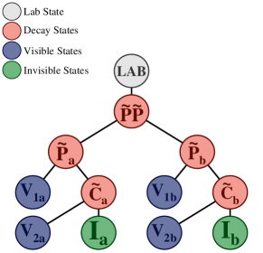
These challenges are examples of kinematic and combinatoric ambiguities appearing in the analysis of particle interactions. In this paper we introduce Recursive Jigsaw Reconstruction (RJR), a technique that can be applied to resolve such unknowns in any production or decay topology of interest, irrespective of their number. The RJR approach analyzes events by factorizing any unknowns according to the different decay steps of intermediate particles expected to appear in an event, making choices for the those associated with each particle decay using a combination of one or more Jigsaw Rules (JR’s), interchangeable and configurable algorithms for resolving individual decays. Each event is then analyzed recursively, iteratively moving from the laboratory frame, where particle four vectors are measured, through each expected intermediate decay frame.

An overview of the RJR approach is provided in Section II, where it is compared to existing HEP event reconstruction strategies. What sets apart the RJR technique is its general applicability achieved through its comprehensive library of JR’s, which includes algorithms for resolving any combination of unknowns that can be encountered. Each of these JR’s are motivated and described in this paper through a series of increasingly complex examples involving a collection of SM and new physics processes at a hadron collider. The notation used throughout this paper is defined in Section III, while the event generator used for simulating the physics processes discussed in each example is described in Section IV.

Twelve different physics examples are considered, organized according to the types of JR’s that are being studied. Section V introduces JR’s for final states with a single invisible particle, including examples with the production and decay of W𝑊W bosons, top quarks, and charged Higgs bosons, as may appear in some extensions of the SM. JR’s for decays with two invisible particles are described in Section VI, with their use demonstrated in examples involving Higgs bosons decaying to W𝑊W’s, and both stop quark and neutralino pair production in SUSY scenarios, with decays through top quarks, Higgs, and Z𝑍Z bosons. To demonstrate how the RJR approach can independently measure the masses of many particles in a single event, examples of resonant and non-resonant top pair production are described in Section VII, with final states containing b𝑏b-quarks, leptons and neutrinos with intermediate W𝑊W bosons. The SUSY analogue of this process, t~t~bχ~±(ν~)bχ~(ν~)~𝑡~𝑡𝑏superscript~𝜒plus-or-minus~𝜈𝑏superscript~𝜒minus-or-plus~𝜈\tilde{t}\tilde{t}\rightarrow b\tilde{\chi}^{\pm}(\ell\tilde{\nu})b\tilde{\chi}^{\mp}(\ell\tilde{\nu}), is also discussed.

JR’s for decays to an arbitrary number of invisible particles are described through the example of non-resonant N2W(ν)𝑁2𝑊𝜈N\geq 2\leavevmode\nobreak\ W(\ell\nu) production in Section VIII, followed by a demonstration of how many JR’s can be combined, recursively, to analyze events with both many kinematic and combinatoric unknowns through the examples Hhh4W(ν)𝐻4𝑊𝜈H\rightarrow hh\rightarrow 4W(\ell\nu) and g~g~bbχ~10bbχ~10~𝑔~𝑔𝑏𝑏subscriptsuperscript~𝜒01𝑏𝑏subscriptsuperscript~𝜒01\tilde{g}\tilde{g}\rightarrow bb\tilde{\chi}^{0}_{1}bb\tilde{\chi}^{0}_{1}.

II Recursive Jigsaw Reconstruction

The RJR approach constitutes both a methodology for analyzing reconstructed particle interactions, and a collection of techniques to resolve combinatorial and kinematic ambiguities, event-by-event, for a given sample.

As used in this paper, event refers to a collection of measurements corresponding to a particle collision, including the three momenta of reconstructed particles and, potentially, additional measurements associated with their masses, missing momentum in one or more directions, or the center-of-mass energy of the interaction. In the RJR approach, a “particle” view of the event is used - in the form of a decay tree diagram - where intermediate heavy states are introduced, decaying to the indivisible “visible” objects, whose four vectors follow from detector particle reconstruction and identification, and “invisible” objects, which correspond to weakly interacting particles hypothesized to have escaped detection.

Each decay tree not only describes how different intermediate states decay to the final state particles in an event, but also implicitly introduces a kinematic basis for analyzing the event; just as the collection of four vectors of all the individual final state particles fully describes an event, so too does the set of all of the masses and decay angles of the particles appearing in a decay tree. The latter is a natural kinematic basis for studying an event, in that the masses of intermediate particles of interest are included, along with decay angles sensitive to their spin and quantum numbers, while other uninformative degrees of freedom (ex. rotational symmetry of an entire event) are clearly isolated.

The number of degrees of freedom associated with a decay tree need not be restricted to just the number of kinematic measurements made in the reconstruction of each event. If there are invisible particles appearing in a decay tree, one or more elements of their kinematic description may be under-constrained. Similarly, some reconstructed particles may be indistinguishable, leading to combinatoric ambiguities related to where each should appear in a decay tree. The masses and decay angles of a decay tree can be thought of as functions of these unknowns, such that the choice of how to analyze an event amounts to specifying how to resolve these under-constrained degrees of freedom.

There have been many strategies proposed for how to resolve kinematic ambiguities on an event-by-event basis. For combinatoric ambiguities, one generally chooses a particular metric to minimize, considering all possible combinatoric assignments, such as intermediate masses, distance metrics like ΔRΔ𝑅\Delta R, and those used in jet clustering. The RJR algorithm uses many of the same concepts, with JR’s designed to make combinatoric assignments which can be combined recursively to treat any number of unknowns.

For kinematic ambiguities associated with invisible or undetected particles, there is a large literature of strategies for measuring the properties of event kinematics despite missing information  Lester:2007fq ; Ross:2007rm ; Cho:2007qv ; Cho:2007dh ; Gripaios:2007is ; Barr:2007hy ; Cheng:2008hk ; Cho:2008cu ; Tovey:2008ui ; Nojiri:2008vq ; Nojiri:2008hy ; Barr:2008ba ; Barr:2008hv ; Cho:2008tj ; Burns:2008va ; Konar:2008ei ; Kim:2009nq ; Barr:2009wu ; Alwall:2009zu ; Barr:2009jv ; Konar:2009wn ; Han:2009ss ; Cho:2009ve ; Barr:2010zj ; Han:2012nm ; Han:2012nr . In these cases, the momentum and masses of invisible particles are unmeasured, and the functional dependence of kinematic quantities of interest on these unknowns must be mitigated.

Some approaches advocate imposing mass constraints on events, solving the associated system of equations for any kinematic unknowns. While potentially useful, such approaches generally involve high-order polynomials, implying many solutions, sometimes with none guaranteed to be real Gripaios:2011jm . Aside from the practical difficulties involved in analyzing data when there is an ensemble of (potentially complex) solutions for each event, there is the additional complication of using such an approach in the context of searches for new particle states, where it can be difficult to guess the masses to include in constraints, or impracticle to include interpretations for many “test” constraints.

Alternatively, under-constrained degrees of freedom that are expected to be small can be ignored, constraining multiple unknowns simultaneously. The efficacy of observables obtained from such an approach depends on the accuracy of the approximation and, as for mass constraints, the existence of real solutions is not guaranteed Rogan:2010kb .

A collection of approaches involve expressing masses of interest as a function of kinematic unknowns, choosing them to minimize or maximize those masses, subject to desired constraints. Examples are MT2subscript𝑀𝑇2M_{T2} Lester:1999tx ; Barr:2003rg , MCTsubscript𝑀𝐶𝑇M_{CT} Nojiri:2007pq ; Polesello:2009rn , and a whole collection of similarly constructed “singularity variables” for estimating masses in final states with two invisible particles Kim:2009si . The key property of these observables is that, if the applied constraints hold, their distribution should bound the true mass from above or below (depending on the minimization or maximization being imposed). Many of the JR’s in the RJR approach use this same strategy, with the important distinction that only a subset of unknowns are considered in each minimization/maximization, with potentially more than one used in a self-consistent reconstruction of a single event.

The observation that motivates the RJR technique is that there is not necessarily only one quantity of interest in each event, but rather, potentially many observables which are useful in concert, and depend on many of the same under-constrained degrees of freedom. This means that in order to ensure that the resulting basis of observables are maximally uncorrelated, care must be taken with how multiple unknowns are parameterized and resolved. In the RJR approach, this is achieved by considering how under-constrained degrees of freedom effect our determination of the velocities relating the different reference frames corresponding to the rest frames of the intermediate states in a given decay tree. We exploit the fact that the measured quantities in an event correspond to a known reference frame, the laboratory frame, and identify the subset of unknowns necessary only for determining the velocity relating it to the next reference frame appearing in the decay tree of interest. Any additional unknowns related to the velocities of subsequent decay frames are considered separately, with the factorization of unknowns repeated recursively through the entirety of a decay tree.

In the RJR framework, an algorithm for resolving the unknowns in a single decay step is called a JR, or jigsaw. Each event is analyzed through the recursive application of a series of JR’s, moving through a decay tree from the lab frame to the rest frame of each intermediate particle appearing in the event. The factorized approach to their use means JR’s are also interchangeable; different JR’s can be chosen to resolve the same unknowns, resulting in different behavior of the derived observables. By considering a subset of unknowns at a time, each JR isolates their effects to only a few observables. The RJR algorithm can be summarized as the application of the following steps:

  1. 1.

    Choose a decay tree to impose on the event, including any intermediate particle states of interest, with measured and invisible particles appearing in the final decay steps.

  2. 2.

    Express the velocity relating the current reference frame to the next one(s) in the decay tree as a function of unknown and measured quantities and choose a JR to resolve these this missing information.

  3. 3.

    Proceed to the subsequent reference frame(s) in the decay tree and repeat (2) until the ends of the tree are reached.

The applied algorithm for analyzing an event is determined by the JR’s that are chosen. Each is based only on an abstraction of the event evaluated in a single reference frame, with at least one JR for each type of decay topology and set of unknowns that can be encountered. The recursive application of JR’s ensures that observables corresponding to different reference frames (masses and decay angles) are maximally uncorrelated from those associated with the frames that precede and follow in the tree.

The RJR framework is simply a library of JR’s which, like puzzle pieces, can be assembled to analyze events according to a chosen decay tree. Each JR resolves unknowns using different constraints and assumptions, with a customizable combination available for studying any process of interest.

III Notation

Throughout this paper, four vectors are denoted in bold, with subscripts indicating the object, or group of objects, to which the four vector corresponds, and superscripts the reference frame the four vector is being evaluated in, such that 𝐩absuperscriptsubscript𝐩ab\mathbf{p}_{\footnotesize\mathrm{{\color[rgb]{0.1,0.1,0.44}\definecolor[named]{pgfstrokecolor}{rgb}{0.1,0.1,0.44}\textbf{a}}}}^{\footnotesize\leavevmode\nobreak\ \mathrm{{\color[rgb]{0.45,0.0,0.09}\definecolor[named]{pgfstrokecolor}{rgb}{0.45,0.0,0.09}\textbf{b}}}} represents the four vector of object a, evaluated in reference frame b. The energy and momentum components of this four vector are denoted by 𝐩ab{Eab,pab}superscriptsubscript𝐩absuperscriptsubscript𝐸absuperscriptsubscript𝑝ab\mathbf{p}_{\footnotesize\mathrm{{\color[rgb]{0.1,0.1,0.44}\definecolor[named]{pgfstrokecolor}{rgb}{0.1,0.1,0.44}\textbf{a}}}}^{\footnotesize\leavevmode\nobreak\ \mathrm{{\color[rgb]{0.45,0.0,0.09}\definecolor[named]{pgfstrokecolor}{rgb}{0.45,0.0,0.09}\textbf{b}}}}\equiv\{E_{\footnotesize\mathrm{{\color[rgb]{0.1,0.1,0.44}\definecolor[named]{pgfstrokecolor}{rgb}{0.1,0.1,0.44}\textbf{a}}}}^{\footnotesize\leavevmode\nobreak\ \mathrm{{\color[rgb]{0.45,0.0,0.09}\definecolor[named]{pgfstrokecolor}{rgb}{0.45,0.0,0.09}\textbf{b}}}},\vec{p}_{\footnotesize\mathrm{{\color[rgb]{0.1,0.1,0.44}\definecolor[named]{pgfstrokecolor}{rgb}{0.1,0.1,0.44}\textbf{a}}}}^{\footnotesize\leavevmode\nobreak\ \mathrm{{\color[rgb]{0.45,0.0,0.09}\definecolor[named]{pgfstrokecolor}{rgb}{0.45,0.0,0.09}\textbf{b}}}}\}, with individual momentum components written pa,xbsuperscriptsubscript𝑝a𝑥bp_{\footnotesize\mathrm{{\color[rgb]{0.1,0.1,0.44}\definecolor[named]{pgfstrokecolor}{rgb}{0.1,0.1,0.44}\textbf{a}}},x}^{\footnotesize\leavevmode\nobreak\ \mathrm{{\color[rgb]{0.45,0.0,0.09}\definecolor[named]{pgfstrokecolor}{rgb}{0.45,0.0,0.09}\textbf{b}}}}.

For readers viewing this paper through a color-sensitive medium, the type of different objects, or collections of objects, is indicated in color: Blue, for objects like a, implies that they are “visible”, with measurements of their four vectors in the lab frame assumed to come from detector reconstruction. “Invisible” particles, corresponding to those that escape detection, are green, while intermediate particle states are shown in red. These labels may also indicate groups of particles. If a represents many individual particles (a{ai,,an}aaian\mathrm{{\color[rgb]{0.1,0.1,0.44}\definecolor[named]{pgfstrokecolor}{rgb}{0.1,0.1,0.44}\textbf{a}}}\equiv\{\mathrm{{\color[rgb]{0.1,0.1,0.44}\definecolor[named]{pgfstrokecolor}{rgb}{0.1,0.1,0.44}\textbf{a${}_{i}$}}},\cdots,\mathrm{{\color[rgb]{0.1,0.1,0.44}\definecolor[named]{pgfstrokecolor}{rgb}{0.1,0.1,0.44}\textbf{a${}_{n}$}}}\}) then it can be used interchangeably to indicate the set of elements in the group or their four vector sum, with 𝐩ab=ia𝐩aibsuperscriptsubscript𝐩absubscriptsuperscripta𝑖superscriptsubscript𝐩aib\mathbf{p}_{\footnotesize\mathrm{{\color[rgb]{0.1,0.1,0.44}\definecolor[named]{pgfstrokecolor}{rgb}{0.1,0.1,0.44}\textbf{a}}}}^{\footnotesize\leavevmode\nobreak\ \mathrm{{\color[rgb]{0.45,0.0,0.09}\definecolor[named]{pgfstrokecolor}{rgb}{0.45,0.0,0.09}\textbf{b}}}}=\sum^{\footnotesize\mathrm{{\color[rgb]{0.1,0.1,0.44}\definecolor[named]{pgfstrokecolor}{rgb}{0.1,0.1,0.44}\textbf{a}}}}_{i}\mathbf{p}_{\footnotesize\mathrm{{\color[rgb]{0.1,0.1,0.44}\definecolor[named]{pgfstrokecolor}{rgb}{0.1,0.1,0.44}\textbf{a${}_{i}$}}}}^{\footnotesize\leavevmode\nobreak\ \mathrm{{\color[rgb]{0.45,0.0,0.09}\definecolor[named]{pgfstrokecolor}{rgb}{0.45,0.0,0.09}\textbf{b}}}}. Similarly, the label of an intermediate particle state is used to represent both the set of invisible and visible particles which follow from the decay of this particle and its four vector. If an intermediate particle b decays to a visible particle a, and invisible particle c, “b” may be used like b{a,c}bac\mathrm{{\color[rgb]{0.45,0.0,0.09}\definecolor[named]{pgfstrokecolor}{rgb}{0.45,0.0,0.09}\textbf{b}}}\equiv\{\mathrm{{\color[rgb]{0.1,0.1,0.44}\definecolor[named]{pgfstrokecolor}{rgb}{0.1,0.1,0.44}\textbf{a}}},\mathrm{{\color[rgb]{0.12,0.3,0.17}\definecolor[named]{pgfstrokecolor}{rgb}{0.12,0.3,0.17}\textbf{c}}}\} or 𝐩bd=𝐩ad+𝐩cdsuperscriptsubscript𝐩bdsuperscriptsubscript𝐩adsuperscriptsubscript𝐩cd\mathbf{p}_{\footnotesize\mathrm{{\color[rgb]{0.45,0.0,0.09}\definecolor[named]{pgfstrokecolor}{rgb}{0.45,0.0,0.09}\textbf{b}}}}^{\footnotesize\leavevmode\nobreak\ \mathrm{{\color[rgb]{0.45,0.0,0.09}\definecolor[named]{pgfstrokecolor}{rgb}{0.45,0.0,0.09}\textbf{d}}}}=\mathbf{p}_{\footnotesize\mathrm{{\color[rgb]{0.1,0.1,0.44}\definecolor[named]{pgfstrokecolor}{rgb}{0.1,0.1,0.44}\textbf{a}}}}^{\footnotesize\leavevmode\nobreak\ \mathrm{{\color[rgb]{0.45,0.0,0.09}\definecolor[named]{pgfstrokecolor}{rgb}{0.45,0.0,0.09}\textbf{d}}}}+\mathbf{p}_{\footnotesize\mathrm{{\color[rgb]{0.12,0.3,0.17}\definecolor[named]{pgfstrokecolor}{rgb}{0.12,0.3,0.17}\textbf{c}}}}^{\footnotesize\leavevmode\nobreak\ \mathrm{{\color[rgb]{0.45,0.0,0.09}\definecolor[named]{pgfstrokecolor}{rgb}{0.45,0.0,0.09}\textbf{d}}}}. Additionally, b can also refer to the rest frame of the object b, with 𝐩bb={mb,0}superscriptsubscript𝐩bbsuperscriptsubscript𝑚babsent0\mathbf{p}_{\footnotesize\mathrm{{\color[rgb]{0.45,0.0,0.09}\definecolor[named]{pgfstrokecolor}{rgb}{0.45,0.0,0.09}\textbf{b}}}}^{\footnotesize\leavevmode\nobreak\ \mathrm{{\color[rgb]{0.45,0.0,0.09}\definecolor[named]{pgfstrokecolor}{rgb}{0.45,0.0,0.09}\textbf{b}}}}=\{m_{\footnotesize\mathrm{{\color[rgb]{0.45,0.0,0.09}\definecolor[named]{pgfstrokecolor}{rgb}{0.45,0.0,0.09}\textbf{b}}}}^{\footnotesize\leavevmode\nobreak\ },\vec{0}\}.

Velocities representing the relative motion of different references frames are expressed as βdbsuperscriptsubscript𝛽db\vec{\beta}_{\footnotesize\mathrm{{\color[rgb]{0.45,0.0,0.09}\definecolor[named]{pgfstrokecolor}{rgb}{0.45,0.0,0.09}\textbf{d}}}}^{\footnotesize\leavevmode\nobreak\ \mathrm{{\color[rgb]{0.45,0.0,0.09}\definecolor[named]{pgfstrokecolor}{rgb}{0.45,0.0,0.09}\textbf{b}}}}, indicating the velocity, in units c𝑐c, of reference frame b in the rest frame of d. βdb=|βdb|superscriptsubscript𝛽dbsuperscriptsubscript𝛽db\beta_{\footnotesize\mathrm{{\color[rgb]{0.45,0.0,0.09}\definecolor[named]{pgfstrokecolor}{rgb}{0.45,0.0,0.09}\textbf{d}}}}^{\footnotesize\leavevmode\nobreak\ \mathrm{{\color[rgb]{0.45,0.0,0.09}\definecolor[named]{pgfstrokecolor}{rgb}{0.45,0.0,0.09}\textbf{b}}}}=|\vec{\beta}_{\footnotesize\mathrm{{\color[rgb]{0.45,0.0,0.09}\definecolor[named]{pgfstrokecolor}{rgb}{0.45,0.0,0.09}\textbf{d}}}}^{\footnotesize\leavevmode\nobreak\ \mathrm{{\color[rgb]{0.45,0.0,0.09}\definecolor[named]{pgfstrokecolor}{rgb}{0.45,0.0,0.09}\textbf{b}}}}| and γdb=[1(βdb)2]1/2superscriptsubscript𝛾dbsuperscriptdelimited-[]1superscriptsuperscriptsubscript𝛽db212\gamma_{\footnotesize\mathrm{{\color[rgb]{0.45,0.0,0.09}\definecolor[named]{pgfstrokecolor}{rgb}{0.45,0.0,0.09}\textbf{d}}}}^{\footnotesize\leavevmode\nobreak\ \mathrm{{\color[rgb]{0.45,0.0,0.09}\definecolor[named]{pgfstrokecolor}{rgb}{0.45,0.0,0.09}\textbf{b}}}}=[1-(\beta_{\footnotesize\mathrm{{\color[rgb]{0.45,0.0,0.09}\definecolor[named]{pgfstrokecolor}{rgb}{0.45,0.0,0.09}\textbf{d}}}}^{\footnotesize\leavevmode\nobreak\ \mathrm{{\color[rgb]{0.45,0.0,0.09}\definecolor[named]{pgfstrokecolor}{rgb}{0.45,0.0,0.09}\textbf{b}}}})^{2}]^{-1/2}. The associated Lorentz transformation is ΛdbsuperscriptsubscriptΛdb\Lambda_{\footnotesize\mathrm{{\color[rgb]{0.45,0.0,0.09}\definecolor[named]{pgfstrokecolor}{rgb}{0.45,0.0,0.09}\textbf{d}}}}^{\footnotesize\leavevmode\nobreak\ \mathrm{{\color[rgb]{0.45,0.0,0.09}\definecolor[named]{pgfstrokecolor}{rgb}{0.45,0.0,0.09}\textbf{b}}}} or ΛβdbsuperscriptsubscriptΛsuperscriptsubscript𝛽dbabsent\Lambda_{\footnotesize\vec{\beta}_{\footnotesize\mathrm{{\color[rgb]{0.45,0.0,0.09}\definecolor[named]{pgfstrokecolor}{rgb}{0.45,0.0,0.09}\textbf{d}}}}^{\footnotesize\leavevmode\nobreak\ \mathrm{{\color[rgb]{0.45,0.0,0.09}\definecolor[named]{pgfstrokecolor}{rgb}{0.45,0.0,0.09}\textbf{b}}}}}^{\footnotesize\leavevmode\nobreak\ }, with Λdb𝐩ad=𝐩absuperscriptsubscriptΛdbsuperscriptsubscript𝐩adsuperscriptsubscript𝐩ab\Lambda_{\footnotesize\mathrm{{\color[rgb]{0.45,0.0,0.09}\definecolor[named]{pgfstrokecolor}{rgb}{0.45,0.0,0.09}\textbf{d}}}}^{\footnotesize\leavevmode\nobreak\ \mathrm{{\color[rgb]{0.45,0.0,0.09}\definecolor[named]{pgfstrokecolor}{rgb}{0.45,0.0,0.09}\textbf{b}}}}\mathbf{p}_{\footnotesize\mathrm{{\color[rgb]{0.1,0.1,0.44}\definecolor[named]{pgfstrokecolor}{rgb}{0.1,0.1,0.44}\textbf{a}}}}^{\footnotesize\leavevmode\nobreak\ \mathrm{{\color[rgb]{0.45,0.0,0.09}\definecolor[named]{pgfstrokecolor}{rgb}{0.45,0.0,0.09}\textbf{d}}}}=\mathbf{p}_{\footnotesize\mathrm{{\color[rgb]{0.1,0.1,0.44}\definecolor[named]{pgfstrokecolor}{rgb}{0.1,0.1,0.44}\textbf{a}}}}^{\footnotesize\leavevmode\nobreak\ \mathrm{{\color[rgb]{0.45,0.0,0.09}\definecolor[named]{pgfstrokecolor}{rgb}{0.45,0.0,0.09}\textbf{b}}}}.

Kinematic observables corresponding to physical quantities, like particle masses or decay angles, always refer to those calculated in the RJR approximate event reconstruction, unless otherwise noted. The “true” values of particles’ masses, on an event-by-event basis (not pole masses), are written in lower case (masuperscriptsubscript𝑚aabsentm_{\footnotesize\mathrm{{\color[rgb]{0.1,0.1,0.44}\definecolor[named]{pgfstrokecolor}{rgb}{0.1,0.1,0.44}\textbf{a}}}}^{\footnotesize\leavevmode\nobreak\ }), while masses calculated to approximate these correct masses are expressed in capital letters (Masuperscriptsubscript𝑀aabsentM_{\footnotesize\mathrm{{\color[rgb]{0.1,0.1,0.44}\definecolor[named]{pgfstrokecolor}{rgb}{0.1,0.1,0.44}\textbf{a}}}}^{\footnotesize\leavevmode\nobreak\ }). Until the relevant JR’s are defined, some observables may depend on unknown quantities which have yet to be specified. These dependencies may be shown explicitly, like Mb(pc,zlab)superscriptsubscript𝑀babsentsuperscriptsubscript𝑝c𝑧labM_{\footnotesize\mathrm{{\color[rgb]{0.45,0.0,0.09}\definecolor[named]{pgfstrokecolor}{rgb}{0.45,0.0,0.09}\textbf{b}}}}^{\footnotesize\leavevmode\nobreak\ }(p_{\footnotesize\mathrm{{\color[rgb]{0.12,0.3,0.17}\definecolor[named]{pgfstrokecolor}{rgb}{0.12,0.3,0.17}\textbf{c}}},z}^{\footnotesize\leavevmode\nobreak\ \mathrm{\textbf{lab}}}), or omitted and discussed in the text. Once JR’s have been chosen and applied, and all unknowns associated with a decay tree have been resolved, these observables represent those calculated with these choices.

Throughout, particle notation is often simplified by referring to particles and anti-particles using the same symbol, or by omitting the charge of particles.

IV Event Generation

Each of the examples described in Sections V-VIII corresponds to a specific production and decay tree, and the RestFrames RestFrames code package is used to generate and analyze Monte Carlo events for each process. Specific code for reproducing each of the examples described in this paper, including all of the figures, is included in the software distribution.

The RestFrames package provides the ability to define fully-configurable decay trees to both generate and analyze reconstructed particle interactions. The event generator includes flat (isotropic) decay kinematics, with options for including phase-space effects from parton distribution functions and particle propagators. This is accomplished through a Markov Chain Monte Carlo (MCMC) scheme, with interchangeable modules available for different types of decays in the tree. No effects from hadronization or imperfect detector resolution are considered; in general, these shortcomings have small effects on the distributions of kinematic observables, as their resolution in correspondence to “true” quantities most strongly depends on the effects of kinematic unknowns. Of greater importance are realistic acceptance requirements on the final state particles assumed to have come from detector reconstruction, which can have large effects on kinematic distributions. These are included in the event generation. The examples in this paper are simulated assuming a qq¯𝑞¯𝑞q\bar{q} initial state at the 13 TeV LHC, using numerical parameterizations of parton distribution functions Martin:2009iq .

Analysis of these events is done using the implementation of the RJR algorithm and JR’s within RestFrames. A configurable decay tree is defined for each view of the event, with corresponding JR’s chosen to resolve any unknowns. RestFrames automates the process of determining whether a decay tree is valid, whether a sufficient number and type of JR’s are specified to resolve all the included unknowns, and the order in which each of the JR’s should be applied to the event. Each particle appearing at any stage in a decay tree is associated with a RestFrames object which, after an event has been analyzed, can be queried about the value of its mass, decay angles, and momentum, evaluated in any reference frame in the reconstructed event.

V Jigsaws for an invisible particle

Whenever a weakly interacting particle is produced in a collider event and escapes undetected, it carries with it irrecoverable kinematic information. In collider experiments, the masses of escaping particles are not directly measured, and their momenta can only be inferred in dimensions where the total momentum is constrained. In this section, we introduce the RJR algorithm through simple examples of event topologies containing a single invisible particle in the final state. The application of JR’s to resolve missing information associated with this particle allows for the accurate extraction of a number of other useful pieces of information from these events.

V.1 Wν𝑊𝜈W\rightarrow\ell\nu at a hadron collider

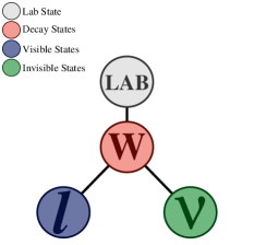
A simple case involving a single invisible particle is the production of a W𝑊W boson with decay Wν𝑊𝜈W\rightarrow\ell\nu, with the decay tree for this process shown in Fig. 1.
Refer to caption
Figure 1: A decay tree diagram for single W𝑊W production and decay. The W𝑊W boson is moving in the lab frame and decays to a lepton and neutrino.

We assume that the lepton is identified and reconstructed by a detector, and that its four vector, 𝐩labsuperscriptsubscript𝐩lab\mathbf{p}_{\footnotesize\mathrm{{\color[rgb]{0.1,0.1,0.44}\definecolor[named]{pgfstrokecolor}{rgb}{0.1,0.1,0.44}\textbf{$\ell$}}}}^{\footnotesize\leavevmode\nobreak\ \mathrm{\textbf{lab}}}, is measured in the lab frame. The neutrino escapes undetected, preventing a direct measurement of its energy and momentum. Exploiting conservation of momentum in the plane transverse to the beam axis, we interpret the measurement of the event missing transverse momentum, ETmisssuperscriptsubscript𝐸𝑇miss\vec{E}_{T}^{\rm miss}, as the transverse momentum of the neutrino, with pν,Tlabsuperscriptsubscript𝑝𝜈𝑇lab\vec{p}_{\footnotesize\mathrm{{\color[rgb]{0.12,0.3,0.17}\definecolor[named]{pgfstrokecolor}{rgb}{0.12,0.3,0.17}\textbf{$\nu$}}},T}^{\footnotesize\leavevmode\nobreak\ \mathrm{\textbf{lab}}} = ETmisssuperscriptsubscript𝐸𝑇miss\vec{E}_{T}^{\rm miss}.

The decay tree shown in Fig. 1 not only describes the event, but also implicitly defines a kinematic basis of useful observables based on this view of the event: the mass, decay angles and lab frame momentum of the W𝑊W boson. Unfortunately, we are unable to calculate any of these quantities from our measurements 𝐩labsuperscriptsubscript𝐩lab\mathbf{p}_{\footnotesize\mathrm{{\color[rgb]{0.1,0.1,0.44}\definecolor[named]{pgfstrokecolor}{rgb}{0.1,0.1,0.44}\textbf{$\ell$}}}}^{\footnotesize\leavevmode\nobreak\ \mathrm{\textbf{lab}}} and pν,Tlabsuperscriptsubscript𝑝𝜈𝑇lab\vec{p}_{\footnotesize\mathrm{{\color[rgb]{0.12,0.3,0.17}\definecolor[named]{pgfstrokecolor}{rgb}{0.12,0.3,0.17}\textbf{$\nu$}}},T}^{\footnotesize\leavevmode\nobreak\ \mathrm{\textbf{lab}}}, as they all also require knowledge of the momentum of the neutrino along the beam axis, pν,zlabsuperscriptsubscript𝑝𝜈𝑧labp_{\footnotesize\mathrm{{\color[rgb]{0.12,0.3,0.17}\definecolor[named]{pgfstrokecolor}{rgb}{0.12,0.3,0.17}\textbf{$\nu$}}},z}^{\footnotesize\leavevmode\nobreak\ \mathrm{\textbf{lab}}}, and its mass, mνsuperscriptsubscript𝑚𝜈absentm_{\footnotesize\mathrm{{\color[rgb]{0.12,0.3,0.17}\definecolor[named]{pgfstrokecolor}{rgb}{0.12,0.3,0.17}\textbf{$\nu$}}}}^{\footnotesize\leavevmode\nobreak\ }, information which is carried with the exiting neutrino.

The shortcomings in our knowledge of the neutrino’s kinematics leave two options: we can either abandon our desired observable basis and restrict our analysis to the quantities we have measured or attempt to resolve, or guess, these unknown quantities using additional constraints. One could, for example, assume that there was an on-shell W𝑊W boson in the event, and require that the invariant mass of the lepton and neutrino be equal to its pole mass. Assuming the neutrino mass is zero, this approach will always result in two solutions for pν,zlabsuperscriptsubscript𝑝𝜈𝑧labp_{\footnotesize\mathrm{{\color[rgb]{0.12,0.3,0.17}\definecolor[named]{pgfstrokecolor}{rgb}{0.12,0.3,0.17}\textbf{$\nu$}}},z}^{\footnotesize\leavevmode\nobreak\ \mathrm{\textbf{lab}}}, with both potentially complex. Apart from the inconvenience of dealing with multiple and complex solutions, such an approach effectively trades any information about the mass of the W𝑊W boson for its momentum and decay kinematics, and is certainly only appropriate as far as its assumptions are valid. The RJR approach also resolves these same unknowns, but does so without any prior assumptions about the masses or decay kinematics of the event, instead using the decay tree to decompose each event into a basis of observables closely approximating those we are interested in.

This is accomplished by considering the under-constrained energy/momentum components of the neutrino instead as unknown components of the velocity relating the lab frame to the W𝑊W rest frame, βWlabsuperscriptsubscript𝛽𝑊lab\vec{\beta}_{\footnotesize\mathrm{{\color[rgb]{0.45,0.0,0.09}\definecolor[named]{pgfstrokecolor}{rgb}{0.45,0.0,0.09}\textbf{$W$}}}}^{\footnotesize\leavevmode\nobreak\ \mathrm{\textbf{lab}}}. Specifying this three vector is equivalent to choosing values pν,zlabsuperscriptsubscript𝑝𝜈𝑧labp_{\footnotesize\mathrm{{\color[rgb]{0.12,0.3,0.17}\definecolor[named]{pgfstrokecolor}{rgb}{0.12,0.3,0.17}\textbf{$\nu$}}},z}^{\footnotesize\leavevmode\nobreak\ \mathrm{\textbf{lab}}} and mνsuperscriptsubscript𝑚𝜈absentm_{\footnotesize\mathrm{{\color[rgb]{0.12,0.3,0.17}\definecolor[named]{pgfstrokecolor}{rgb}{0.12,0.3,0.17}\textbf{$\nu$}}}}^{\footnotesize\leavevmode\nobreak\ }, and sufficient for calculating an approximation of any quantity of interest in the event: It can be used to boost the measured lepton to the W𝑊W frame, and to calculate the W𝑊W decay angle (cosθW=β^Wlabp^W)cossubscript𝜃Wsuperscriptsubscript^𝛽Wlabsuperscriptsubscript^𝑝W(\mathrm{cos}\leavevmode\nobreak\ \theta_{\mathrm{{\color[rgb]{0.45,0.0,0.09}\definecolor[named]{pgfstrokecolor}{rgb}{0.45,0.0,0.09}\textbf{\it W}}}}=\hat{\beta}_{\footnotesize\mathrm{{\color[rgb]{0.45,0.0,0.09}\definecolor[named]{pgfstrokecolor}{rgb}{0.45,0.0,0.09}\textbf{\it W}}}}^{\footnotesize\leavevmode\nobreak\ \mathrm{\textbf{lab}}}\cdot\hat{p}_{\footnotesize\mathrm{{\color[rgb]{0.1,0.1,0.44}\definecolor[named]{pgfstrokecolor}{rgb}{0.1,0.1,0.44}\textbf{$\ell$}}}}^{\footnotesize\leavevmode\nobreak\ \mathrm{{\color[rgb]{0.45,0.0,0.09}\definecolor[named]{pgfstrokecolor}{rgb}{0.45,0.0,0.09}\textbf{\it W}}}}), compare the azimuthal orientation of the W𝑊W decay plane to the W𝑊W momentum and beam axis plane (ΔϕW=p^W×β^Wlabn^z×β^WlabΔsubscriptitalic-ϕWsuperscriptsubscript^𝑝Wsuperscriptsubscript^𝛽Wlabsubscript^𝑛zsuperscriptsubscript^𝛽Wlab\Delta\phi_{\mathrm{{\color[rgb]{0.45,0.0,0.09}\definecolor[named]{pgfstrokecolor}{rgb}{0.45,0.0,0.09}\textbf{\it W}}}}=\hat{p}_{\footnotesize\mathrm{{\color[rgb]{0.1,0.1,0.44}\definecolor[named]{pgfstrokecolor}{rgb}{0.1,0.1,0.44}\textbf{$\ell$}}}}^{\footnotesize\leavevmode\nobreak\ \mathrm{{\color[rgb]{0.45,0.0,0.09}\definecolor[named]{pgfstrokecolor}{rgb}{0.45,0.0,0.09}\textbf{\it W}}}}\times\hat{\beta}_{\footnotesize\mathrm{{\color[rgb]{0.45,0.0,0.09}\definecolor[named]{pgfstrokecolor}{rgb}{0.45,0.0,0.09}\textbf{\it W}}}}^{\footnotesize\leavevmode\nobreak\ \mathrm{\textbf{lab}}}\leavevmode\nobreak\ \angle\leavevmode\nobreak\ \hat{n}_{\mathrm{z}}\times\hat{\beta}_{\footnotesize\mathrm{{\color[rgb]{0.45,0.0,0.09}\definecolor[named]{pgfstrokecolor}{rgb}{0.45,0.0,0.09}\textbf{\it W}}}}^{\footnotesize\leavevmode\nobreak\ \mathrm{\textbf{lab}}}), and measure the W𝑊W mass (EW=MW 2mν 2+m 22MW)superscriptsubscript𝐸Wsuperscriptsubscript𝑀W2superscriptsubscript𝑚𝜈2superscriptsubscript𝑚22superscriptsubscript𝑀Wabsent(E_{\footnotesize\mathrm{{\color[rgb]{0.1,0.1,0.44}\definecolor[named]{pgfstrokecolor}{rgb}{0.1,0.1,0.44}\textbf{$\ell$}}}}^{\footnotesize\leavevmode\nobreak\ \mathrm{{\color[rgb]{0.45,0.0,0.09}\definecolor[named]{pgfstrokecolor}{rgb}{0.45,0.0,0.09}\textbf{\it W}}}}=\frac{M_{\footnotesize\mathrm{{\color[rgb]{0.45,0.0,0.09}\definecolor[named]{pgfstrokecolor}{rgb}{0.45,0.0,0.09}\textbf{\it W}}}}^{\footnotesize\leavevmode\nobreak\ 2}-m_{\footnotesize\mathrm{{\color[rgb]{0.12,0.3,0.17}\definecolor[named]{pgfstrokecolor}{rgb}{0.12,0.3,0.17}\textbf{$\nu$}}}}^{\footnotesize\leavevmode\nobreak\ 2}+m_{\footnotesize\mathrm{{\color[rgb]{0.1,0.1,0.44}\definecolor[named]{pgfstrokecolor}{rgb}{0.1,0.1,0.44}\textbf{$\ell$}}}}^{\footnotesize\leavevmode\nobreak\ 2}}{2M_{\footnotesize\mathrm{{\color[rgb]{0.45,0.0,0.09}\definecolor[named]{pgfstrokecolor}{rgb}{0.45,0.0,0.09}\textbf{\it W}}}}^{\footnotesize\leavevmode\nobreak\ }}). This is true in general, where the measured four vectors of visible particles and the velocities relating adjacent reference frames fully specify the kinematics of a decay tree.

When choosing the unknown components of βWlabsuperscriptsubscript𝛽𝑊lab\vec{\beta}_{\footnotesize\mathrm{{\color[rgb]{0.45,0.0,0.09}\definecolor[named]{pgfstrokecolor}{rgb}{0.45,0.0,0.09}\textbf{$W$}}}}^{\footnotesize\leavevmode\nobreak\ \mathrm{\textbf{lab}}} we decompose this velocity into two pieces: βW,zlabsuperscriptsubscript𝛽𝑊𝑧lab\beta_{\footnotesize\mathrm{{\color[rgb]{0.45,0.0,0.09}\definecolor[named]{pgfstrokecolor}{rgb}{0.45,0.0,0.09}\textbf{$W$}}},z}^{\footnotesize\leavevmode\nobreak\ \mathrm{\textbf{lab}}}, the longitudinal boost to a reference frame, lab,zlab𝑧\mathrm{\textbf{lab}},z, where pW,zlab,z=0superscriptsubscript𝑝𝑊𝑧lab𝑧0p_{\footnotesize\mathrm{{\color[rgb]{0.45,0.0,0.09}\definecolor[named]{pgfstrokecolor}{rgb}{0.45,0.0,0.09}\textbf{$W$}}},z}^{\footnotesize\leavevmode\nobreak\ \mathrm{\textbf{lab}},z}=0, and βW,Tlab,zsuperscriptsubscript𝛽𝑊𝑇lab𝑧\vec{\beta}_{\footnotesize\mathrm{{\color[rgb]{0.45,0.0,0.09}\definecolor[named]{pgfstrokecolor}{rgb}{0.45,0.0,0.09}\textbf{$W$}}},T}^{\footnotesize\leavevmode\nobreak\ \mathrm{\textbf{lab}},z}, the transverse velocity relating that intermediate frame to the W𝑊W rest frame. For the first of these velocities, rather than trying to make the most accurate guess (by, for example, using likelihoods sensitive to parton distribution functions) we choose a value that ensures that any quantities we calculate using our guess are independent of the true value. This is ensured by choosing βW,zlabsuperscriptsubscript𝛽𝑊𝑧lab\beta_{\footnotesize\mathrm{{\color[rgb]{0.45,0.0,0.09}\definecolor[named]{pgfstrokecolor}{rgb}{0.45,0.0,0.09}\textbf{$W$}}},z}^{\footnotesize\leavevmode\nobreak\ \mathrm{\textbf{lab}}} to satisfy

Elab,z(βW,zlab)βW,zlab=0,superscriptsubscript𝐸lab𝑧superscriptsubscript𝛽𝑊𝑧labsuperscriptsubscript𝛽𝑊𝑧lab0\frac{\partial E_{\footnotesize\mathrm{{\color[rgb]{0.1,0.1,0.44}\definecolor[named]{pgfstrokecolor}{rgb}{0.1,0.1,0.44}\textbf{$\ell$}}}}^{\footnotesize\leavevmode\nobreak\ \mathrm{\textbf{lab}},z}(\beta_{\footnotesize\mathrm{{\color[rgb]{0.45,0.0,0.09}\definecolor[named]{pgfstrokecolor}{rgb}{0.45,0.0,0.09}\textbf{$W$}}},z}^{\footnotesize\leavevmode\nobreak\ \mathrm{\textbf{lab}}})}{\partial\beta_{\footnotesize\mathrm{{\color[rgb]{0.45,0.0,0.09}\definecolor[named]{pgfstrokecolor}{rgb}{0.45,0.0,0.09}\textbf{$W$}}},z}^{\footnotesize\leavevmode\nobreak\ \mathrm{\textbf{lab}}}}=0\leavevmode\nobreak\ , (1)

such that βW,zlab=p,zlab/Elabsuperscriptsubscript𝛽W𝑧labsuperscriptsubscript𝑝𝑧labsuperscriptsubscript𝐸lab\beta_{\footnotesize\mathrm{{\color[rgb]{0.45,0.0,0.09}\definecolor[named]{pgfstrokecolor}{rgb}{0.45,0.0,0.09}\textbf{\it W}}},z}^{\footnotesize\leavevmode\nobreak\ \mathrm{\textbf{lab}}}=p_{\footnotesize\mathrm{{\color[rgb]{0.1,0.1,0.44}\definecolor[named]{pgfstrokecolor}{rgb}{0.1,0.1,0.44}\textbf{$\ell$}}},z}^{\footnotesize\leavevmode\nobreak\ \mathrm{\textbf{lab}}}/E_{\footnotesize\mathrm{{\color[rgb]{0.1,0.1,0.44}\definecolor[named]{pgfstrokecolor}{rgb}{0.1,0.1,0.44}\textbf{$\ell$}}}}^{\footnotesize\leavevmode\nobreak\ \mathrm{\textbf{lab}}}. This choice also sets pν,zlabsuperscriptsubscript𝑝𝜈𝑧labp_{\footnotesize\mathrm{{\color[rgb]{0.12,0.3,0.17}\definecolor[named]{pgfstrokecolor}{rgb}{0.12,0.3,0.17}\textbf{$\nu$}}},z}^{\footnotesize\leavevmode\nobreak\ \mathrm{\textbf{lab}}}, with pν,zlab,z=p,zlab,z=pW,zlab,z=0superscriptsubscript𝑝𝜈𝑧lab𝑧superscriptsubscript𝑝𝑧lab𝑧superscriptsubscript𝑝𝑊𝑧lab𝑧0p_{\footnotesize\mathrm{{\color[rgb]{0.12,0.3,0.17}\definecolor[named]{pgfstrokecolor}{rgb}{0.12,0.3,0.17}\textbf{$\nu$}}},z}^{\footnotesize\leavevmode\nobreak\ \mathrm{\textbf{lab}},z}=p_{\footnotesize\mathrm{{\color[rgb]{0.1,0.1,0.44}\definecolor[named]{pgfstrokecolor}{rgb}{0.1,0.1,0.44}\textbf{$\ell$}}},z}^{\footnotesize\leavevmode\nobreak\ \mathrm{\textbf{lab}},z}=p_{\footnotesize\mathrm{{\color[rgb]{0.45,0.0,0.09}\definecolor[named]{pgfstrokecolor}{rgb}{0.45,0.0,0.09}\textbf{$W$}}},z}^{\footnotesize\leavevmode\nobreak\ \mathrm{\textbf{lab}},z}=0, and is equivalent to setting the rapidity of the neutrino equal to that of the lepton. This algorithmic determination of βW,zlabsuperscriptsubscript𝛽W𝑧lab\beta_{\footnotesize\mathrm{{\color[rgb]{0.45,0.0,0.09}\definecolor[named]{pgfstrokecolor}{rgb}{0.45,0.0,0.09}\textbf{\it W}}},z}^{\footnotesize\leavevmode\nobreak\ \mathrm{\textbf{lab}}} is an example of a JR, where a guess for an unknown quantity is made based on the four momenta of visible particles, evaluated in a particular reference frame:

Jigsaw Rule V.1 (Invisible Rapidity)

If the momentum of an invisible particle, I, in a reference frame, F, is unknown along an axis n^subscript^𝑛parallel-to\hat{n}_{\parallel}, it can be chosen such that the rapidity of I along n^subscript^𝑛parallel-to\hat{n}_{\parallel} is set equal to that of a visible system of particles V according to:

pI,F=pV,F|pI,F|2+mI 2|pV,F|2+mV 2,p_{\footnotesize\mathrm{{\color[rgb]{0.12,0.3,0.17}\definecolor[named]{pgfstrokecolor}{rgb}{0.12,0.3,0.17}\textbf{I}}},\parallel}^{\footnotesize\leavevmode\nobreak\ \mathrm{{\color[rgb]{0.45,0.0,0.09}\definecolor[named]{pgfstrokecolor}{rgb}{0.45,0.0,0.09}\textbf{F}}}}=p_{\footnotesize\mathrm{{\color[rgb]{0.1,0.1,0.44}\definecolor[named]{pgfstrokecolor}{rgb}{0.1,0.1,0.44}\textbf{V}}},\parallel}^{\footnotesize\leavevmode\nobreak\ \mathrm{{\color[rgb]{0.45,0.0,0.09}\definecolor[named]{pgfstrokecolor}{rgb}{0.45,0.0,0.09}\textbf{F}}}}\frac{\sqrt{|\vec{p}_{\footnotesize\mathrm{{\color[rgb]{0.12,0.3,0.17}\definecolor[named]{pgfstrokecolor}{rgb}{0.12,0.3,0.17}\textbf{I}}},\perp}^{\footnotesize\leavevmode\nobreak\ \mathrm{{\color[rgb]{0.45,0.0,0.09}\definecolor[named]{pgfstrokecolor}{rgb}{0.45,0.0,0.09}\textbf{F}}}}|^{2}+m_{\footnotesize\mathrm{{\color[rgb]{0.12,0.3,0.17}\definecolor[named]{pgfstrokecolor}{rgb}{0.12,0.3,0.17}\textbf{I}}}}^{\footnotesize\leavevmode\nobreak\ 2}}}{\sqrt{|\vec{p}_{\footnotesize\mathrm{{\color[rgb]{0.1,0.1,0.44}\definecolor[named]{pgfstrokecolor}{rgb}{0.1,0.1,0.44}\textbf{V}}},\perp}^{\footnotesize\leavevmode\nobreak\ \mathrm{{\color[rgb]{0.45,0.0,0.09}\definecolor[named]{pgfstrokecolor}{rgb}{0.45,0.0,0.09}\textbf{F}}}}|^{2}+m_{\footnotesize\mathrm{{\color[rgb]{0.1,0.1,0.44}\definecolor[named]{pgfstrokecolor}{rgb}{0.1,0.1,0.44}\textbf{V}}}}^{\footnotesize\leavevmode\nobreak\ 2}}}\leavevmode\nobreak\ , (2)

where “perpendicular-to\perp” indicates the plane normal to n^subscript^𝑛parallel-to\hat{n}_{\parallel}. This choice is equivalent to minimizing MVIsuperscriptsubscript𝑀VIabsentM_{\footnotesize\mathrm{{\color[rgb]{0.1,0.1,0.44}\definecolor[named]{pgfstrokecolor}{rgb}{0.1,0.1,0.44}\textbf{V}}}\mathrm{{\color[rgb]{0.12,0.3,0.17}\definecolor[named]{pgfstrokecolor}{rgb}{0.12,0.3,0.17}\textbf{I}}}}^{\footnotesize\leavevmode\nobreak\ } w.r.t. pI,Fp_{\footnotesize\mathrm{{\color[rgb]{0.12,0.3,0.17}\definecolor[named]{pgfstrokecolor}{rgb}{0.12,0.3,0.17}\textbf{I}}},\parallel}^{\footnotesize\leavevmode\nobreak\ \mathrm{{\color[rgb]{0.45,0.0,0.09}\definecolor[named]{pgfstrokecolor}{rgb}{0.45,0.0,0.09}\textbf{F}}}}.

That the application of JR V.1 ensures that all observables depending on βW,zlabsuperscriptsubscript𝛽W𝑧lab\beta_{\footnotesize\mathrm{{\color[rgb]{0.45,0.0,0.09}\definecolor[named]{pgfstrokecolor}{rgb}{0.45,0.0,0.09}\textbf{\it W}}},z}^{\footnotesize\leavevmode\nobreak\ \mathrm{\textbf{lab}}} are independent of its true value (or, alternatively, that they are invariant under longitudinal boosts in the lab frame) can be understood intuitively by noting that our definition of the lab,z reference frame is itself longitudinally boost invariant, in that we will always arrive at the same lab,zlab𝑧\mathrm{\textbf{lab}},z irrespective of the W𝑊W boson’s velocity along the beam axis. As all subsequent estimators (and choices for other unknowns) follow from the choices made in this frame, in a sense observables associated with reference frames appearing below lab,zlab𝑧\mathrm{\textbf{lab}},z in the decay tree inherit this invariance property.

With βW,zlabsuperscriptsubscript𝛽W𝑧lab\beta_{\footnotesize\mathrm{{\color[rgb]{0.45,0.0,0.09}\definecolor[named]{pgfstrokecolor}{rgb}{0.45,0.0,0.09}\textbf{\it W}}},z}^{\footnotesize\leavevmode\nobreak\ \mathrm{\textbf{lab}}} specified, we need to guess the remaining velocity βW,Tlab,zsuperscriptsubscript𝛽𝑊𝑇lab𝑧\vec{\beta}_{\footnotesize\mathrm{{\color[rgb]{0.45,0.0,0.09}\definecolor[named]{pgfstrokecolor}{rgb}{0.45,0.0,0.09}\textbf{$W$}}},T}^{\footnotesize\leavevmode\nobreak\ \mathrm{\textbf{lab}},z}, whose magnitude depends on mνsuperscriptsubscript𝑚𝜈absentm_{\footnotesize\mathrm{{\color[rgb]{0.12,0.3,0.17}\definecolor[named]{pgfstrokecolor}{rgb}{0.12,0.3,0.17}\textbf{$\nu$}}}}^{\footnotesize\leavevmode\nobreak\ }. We could attempt to specify this unknown using a similar approach to βW,zlabsuperscriptsubscript𝛽W𝑧lab\beta_{\footnotesize\mathrm{{\color[rgb]{0.45,0.0,0.09}\definecolor[named]{pgfstrokecolor}{rgb}{0.45,0.0,0.09}\textbf{\it W}}},z}^{\footnotesize\leavevmode\nobreak\ \mathrm{\textbf{lab}}}, for example choosing βW,Tlab,zsuperscriptsubscript𝛽𝑊𝑇lab𝑧\beta_{\footnotesize\mathrm{{\color[rgb]{0.45,0.0,0.09}\definecolor[named]{pgfstrokecolor}{rgb}{0.45,0.0,0.09}\textbf{$W$}}},T}^{\footnotesize\leavevmode\nobreak\ \mathrm{\textbf{lab}},z} to minimize MWsuperscriptsubscript𝑀𝑊absentM_{\footnotesize\mathrm{{\color[rgb]{0.45,0.0,0.09}\definecolor[named]{pgfstrokecolor}{rgb}{0.45,0.0,0.09}\textbf{$W$}}}}^{\footnotesize\leavevmode\nobreak\ }. Unfortunately, this can result in unphysical values of Mνsuperscriptsubscript𝑀𝜈absentM_{\footnotesize\mathrm{{\color[rgb]{0.12,0.3,0.17}\definecolor[named]{pgfstrokecolor}{rgb}{0.12,0.3,0.17}\textbf{$\nu$}}}}^{\footnotesize\leavevmode\nobreak\ }, with a tachyonic reconstructed neutrino. This is true in general for the individual masses of invisible particles, in that partial derivatives of derived quantities w.r.t. these masses are never guaranteed to be physically viable. In this case, we set Mν=0superscriptsubscript𝑀𝜈absent0M_{\footnotesize\mathrm{{\color[rgb]{0.12,0.3,0.17}\definecolor[named]{pgfstrokecolor}{rgb}{0.12,0.3,0.17}\textbf{$\nu$}}}}^{\footnotesize\leavevmode\nobreak\ }=0 both because the neutrino mass is negligible on the scale of this event and because it is the smallest Lorentz invariant choice which guarantees a viable interpretation of the event. The importance of this latter distinction will become clear in later examples with multiple invisible particles in the final state.

Once values for the unknowns associated with the neutrino have been specified, we can calculate any observable of interest in our approximate view of the event. Our estimator for the W𝑊W mass can be expressed in terms of measurable quantities in the lab frame:

MW 2superscriptsubscript𝑀W2\displaystyle M_{\footnotesize\mathrm{{\color[rgb]{0.45,0.0,0.09}\definecolor[named]{pgfstrokecolor}{rgb}{0.45,0.0,0.09}\textbf{\it W}}}}^{\footnotesize\leavevmode\nobreak\ 2} =\displaystyle=
m 2superscriptsubscript𝑚2\displaystyle m_{\footnotesize\mathrm{{\color[rgb]{0.1,0.1,0.44}\definecolor[named]{pgfstrokecolor}{rgb}{0.1,0.1,0.44}\textbf{$\ell$}}}}^{\footnotesize\leavevmode\nobreak\ 2} +\displaystyle+ 2(|pν,Tlab|m 2+|p,Tlab|2p,Tlabpν,Tlab),2superscriptsubscript𝑝𝜈𝑇labsuperscriptsubscript𝑚2superscriptsuperscriptsubscript𝑝𝑇lab2superscriptsubscript𝑝𝑇labsuperscriptsubscript𝑝𝜈𝑇lab\displaystyle 2\left(|\vec{p}_{\footnotesize\mathrm{{\color[rgb]{0.12,0.3,0.17}\definecolor[named]{pgfstrokecolor}{rgb}{0.12,0.3,0.17}\textbf{$\nu$}}},T}^{\footnotesize\leavevmode\nobreak\ \mathrm{\textbf{lab}}}|\sqrt{m_{\footnotesize\mathrm{{\color[rgb]{0.1,0.1,0.44}\definecolor[named]{pgfstrokecolor}{rgb}{0.1,0.1,0.44}\textbf{$\ell$}}}}^{\footnotesize\leavevmode\nobreak\ 2}+|\vec{p}_{\footnotesize\mathrm{{\color[rgb]{0.1,0.1,0.44}\definecolor[named]{pgfstrokecolor}{rgb}{0.1,0.1,0.44}\textbf{$\ell$}}},T}^{\footnotesize\leavevmode\nobreak\ \mathrm{\textbf{lab}}}|^{2}}-\vec{p}_{\footnotesize\mathrm{{\color[rgb]{0.1,0.1,0.44}\definecolor[named]{pgfstrokecolor}{rgb}{0.1,0.1,0.44}\textbf{$\ell$}}},T}^{\footnotesize\leavevmode\nobreak\ \mathrm{\textbf{lab}}}\cdot\vec{p}_{\footnotesize\mathrm{{\color[rgb]{0.12,0.3,0.17}\definecolor[named]{pgfstrokecolor}{rgb}{0.12,0.3,0.17}\textbf{$\nu$}}},T}^{\footnotesize\leavevmode\nobreak\ \mathrm{\textbf{lab}}}\right)\leavevmode\nobreak\ , (3)

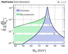
where we note that we have re-derived the transverse mass. The distribution of MWsuperscriptsubscript𝑀WabsentM_{\footnotesize\mathrm{{\color[rgb]{0.45,0.0,0.09}\definecolor[named]{pgfstrokecolor}{rgb}{0.45,0.0,0.09}\textbf{\it W}}}}^{\footnotesize\leavevmode\nobreak\ } is shown in Fig. 2(a), where we observe MWmWsuperscriptsubscript𝑀Wabsentsuperscriptsubscript𝑚WabsentM_{\footnotesize\mathrm{{\color[rgb]{0.45,0.0,0.09}\definecolor[named]{pgfstrokecolor}{rgb}{0.45,0.0,0.09}\textbf{\it W}}}}^{\footnotesize\leavevmode\nobreak\ }\leq m_{\footnotesize\mathrm{{\color[rgb]{0.45,0.0,0.09}\definecolor[named]{pgfstrokecolor}{rgb}{0.45,0.0,0.09}\textbf{\it W}}}}^{\footnotesize\leavevmode\nobreak\ }, due to our implicit minimization in our choice of pν,zlabsuperscriptsubscript𝑝𝜈𝑧labp_{\footnotesize\mathrm{{\color[rgb]{0.12,0.3,0.17}\definecolor[named]{pgfstrokecolor}{rgb}{0.12,0.3,0.17}\textbf{$\nu$}}},z}^{\footnotesize\leavevmode\nobreak\ \mathrm{\textbf{lab}}}.

Refer to caption
Refer to caption
Refer to caption
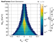
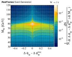
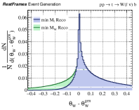
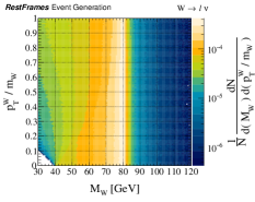
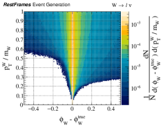
Figure 2: (a) Distribution of MWsuperscriptsubscript𝑀WabsentM_{\footnotesize\mathrm{{\color[rgb]{0.45,0.0,0.09}\definecolor[named]{pgfstrokecolor}{rgb}{0.45,0.0,0.09}\textbf{\it W}}}}^{\footnotesize\leavevmode\nobreak\ } for simulated Wν𝑊𝜈W\rightarrow\ell\nu events at both generator level and after reconstruction. Each distribution is normalized to unit area. Distributions of (b) azimuthal component of the W𝑊W decay angle, ϕWsubscriptitalic-ϕW\phi_{\mathrm{{\color[rgb]{0.45,0.0,0.09}\definecolor[named]{pgfstrokecolor}{rgb}{0.45,0.0,0.09}\textbf{\it W}}}}, and (c) ΔϕWΔsubscriptitalic-ϕW\Delta\phi_{\mathrm{{\color[rgb]{0.45,0.0,0.09}\definecolor[named]{pgfstrokecolor}{rgb}{0.45,0.0,0.09}\textbf{\it W}}}}, relative to their true values, compared with the reconstructed W𝑊W mass. Angles are shown in units radian.

In addition to MWsuperscriptsubscript𝑀WabsentM_{\footnotesize\mathrm{{\color[rgb]{0.45,0.0,0.09}\definecolor[named]{pgfstrokecolor}{rgb}{0.45,0.0,0.09}\textbf{\it W}}}}^{\footnotesize\leavevmode\nobreak\ }, we can also calculate estimators of other quantities of interest in the event. Distributions for the azimuthal component of the W𝑊W decay angle, ϕWsubscriptitalic-ϕ𝑊\phi_{\mathrm{{\color[rgb]{0.45,0.0,0.09}\definecolor[named]{pgfstrokecolor}{rgb}{0.45,0.0,0.09}\textbf{$W$}}}}, and ΔϕWΔsubscriptitalic-ϕW\Delta\phi_{\mathrm{{\color[rgb]{0.45,0.0,0.09}\definecolor[named]{pgfstrokecolor}{rgb}{0.45,0.0,0.09}\textbf{\it W}}}} are shown in Fig. 2(b,c), where the differences between the reconstructed and true quantities for these observables are examined as a function of MWsuperscriptsubscript𝑀WabsentM_{\footnotesize\mathrm{{\color[rgb]{0.45,0.0,0.09}\definecolor[named]{pgfstrokecolor}{rgb}{0.45,0.0,0.09}\textbf{\it W}}}}^{\footnotesize\leavevmode\nobreak\ }. We observe that both ϕWsubscriptitalic-ϕ𝑊\phi_{\mathrm{{\color[rgb]{0.45,0.0,0.09}\definecolor[named]{pgfstrokecolor}{rgb}{0.45,0.0,0.09}\textbf{$W$}}}} and ΔϕWΔsubscriptitalic-ϕW\Delta\phi_{\mathrm{{\color[rgb]{0.45,0.0,0.09}\definecolor[named]{pgfstrokecolor}{rgb}{0.45,0.0,0.09}\textbf{\it W}}}} can be reconstructed with excellent resolution, and largely independently of MWsuperscriptsubscript𝑀WabsentM_{\footnotesize\mathrm{{\color[rgb]{0.45,0.0,0.09}\definecolor[named]{pgfstrokecolor}{rgb}{0.45,0.0,0.09}\textbf{\it W}}}}^{\footnotesize\leavevmode\nobreak\ }, despite the missing information associated with the neutrino.

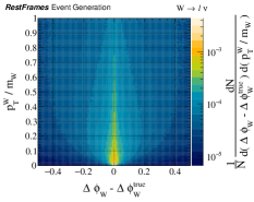
Not only are these estimators nearly entirely independent from each other, but they are almost entirely insensitive to the true momentum of the W𝑊W boson in the lab frame. In addition to being manifestly invariant under longitudinal boosts, the reconstructed quantities MWsuperscriptsubscript𝑀WabsentM_{\footnotesize\mathrm{{\color[rgb]{0.45,0.0,0.09}\definecolor[named]{pgfstrokecolor}{rgb}{0.45,0.0,0.09}\textbf{\it W}}}}^{\footnotesize\leavevmode\nobreak\ }, ϕWsubscriptitalic-ϕ𝑊\phi_{\mathrm{{\color[rgb]{0.45,0.0,0.09}\definecolor[named]{pgfstrokecolor}{rgb}{0.45,0.0,0.09}\textbf{$W$}}}}, and ΔϕWΔsubscriptitalic-ϕW\Delta\phi_{\mathrm{{\color[rgb]{0.45,0.0,0.09}\definecolor[named]{pgfstrokecolor}{rgb}{0.45,0.0,0.09}\textbf{\it W}}}} have almost no dependence on the W𝑊W transverse momentum, as demonstrated in Fig. 3. The RJR analysis prescription for these events results in a basis of observables, each with a strong correspondence to the true value of the quantity it is estimating, and little correlation between them introduced by the reconstruction algorithm.
Refer to caption
Refer to caption
Refer to caption
Figure 3: Distributions of (a) the reconstructed W𝑊W mass, MWsuperscriptsubscript𝑀WabsentM_{\footnotesize\mathrm{{\color[rgb]{0.45,0.0,0.09}\definecolor[named]{pgfstrokecolor}{rgb}{0.45,0.0,0.09}\textbf{\it W}}}}^{\footnotesize\leavevmode\nobreak\ }, (b) the azimuthal component of the W𝑊W decay angle, ϕWsubscriptitalic-ϕW\phi_{\mathrm{{\color[rgb]{0.45,0.0,0.09}\definecolor[named]{pgfstrokecolor}{rgb}{0.45,0.0,0.09}\textbf{\it W}}}}, and (c) ΔϕWΔsubscriptitalic-ϕW\Delta\phi_{\mathrm{{\color[rgb]{0.45,0.0,0.09}\definecolor[named]{pgfstrokecolor}{rgb}{0.45,0.0,0.09}\textbf{\it W}}}}, shown as a function of pW,Tlab/mWsuperscriptsubscript𝑝W𝑇labsuperscriptsubscript𝑚Wabsentp_{\footnotesize\mathrm{{\color[rgb]{0.45,0.0,0.09}\definecolor[named]{pgfstrokecolor}{rgb}{0.45,0.0,0.09}\textbf{\it W}}},T}^{\footnotesize\leavevmode\nobreak\ \mathrm{\textbf{lab}}}/m_{\footnotesize\mathrm{{\color[rgb]{0.45,0.0,0.09}\definecolor[named]{pgfstrokecolor}{rgb}{0.45,0.0,0.09}\textbf{\it W}}}}^{\footnotesize\leavevmode\nobreak\ }, for simulated Wν𝑊𝜈W\rightarrow\ell\nu events. Angles are shown in units radian.

V.2 Single-top production with tbW(ν)𝑡𝑏𝑊𝜈t\rightarrow bW(\ell\nu)

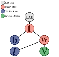
We expand on the previous example by considering the case of single-top production at a hadron collider, with subsequent decay to a b𝑏b-quark, lepton, and neutrino, via an intermediate W𝑊W boson. The decay tree for analysis of this final state is shown in Fig. 4. As in Section V.1, we assume that the lepton four vector, 𝐩labsuperscriptsubscript𝐩lab\mathbf{p}_{\footnotesize\mathrm{{\color[rgb]{0.1,0.1,0.44}\definecolor[named]{pgfstrokecolor}{rgb}{0.1,0.1,0.44}\textbf{$\ell$}}}}^{\footnotesize\leavevmode\nobreak\ \mathrm{\textbf{lab}}}, and transverse momentum of the neutrino, pν,Tlabsuperscriptsubscript𝑝𝜈𝑇lab\vec{p}_{\footnotesize\mathrm{{\color[rgb]{0.12,0.3,0.17}\definecolor[named]{pgfstrokecolor}{rgb}{0.12,0.3,0.17}\textbf{$\nu$}}},T}^{\footnotesize\leavevmode\nobreak\ \mathrm{\textbf{lab}}}, are measured in the lab frame, with an additional b𝑏b-tagged jet associated with the final state b𝑏b-quark also reconstructed, with four vector 𝐩blabsuperscriptsubscript𝐩𝑏lab\mathbf{p}_{\footnotesize\mathrm{{\color[rgb]{0.1,0.1,0.44}\definecolor[named]{pgfstrokecolor}{rgb}{0.1,0.1,0.44}\textbf{$b$}}}}^{\footnotesize\leavevmode\nobreak\ \mathrm{\textbf{lab}}}.

Refer to caption
Figure 4: A decay tree diagram for a single top quark decaying to a b𝑏b-quark, lepton, and neutrino, through an intermediate W𝑊W boson.
Refer to caption
Refer to caption
Refer to caption
Refer to caption
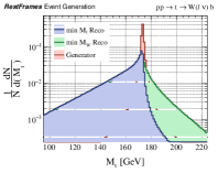
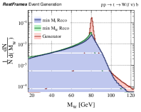
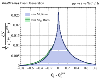
Figure 5: Distributions of reconstructed (a) top quark mass, Mtsuperscriptsubscript𝑀𝑡absentM_{\footnotesize\mathrm{{\color[rgb]{0.45,0.0,0.09}\definecolor[named]{pgfstrokecolor}{rgb}{0.45,0.0,0.09}\textbf{$t$}}}}^{\footnotesize\leavevmode\nobreak\ }, (b) W𝑊W boson mass, MWsuperscriptsubscript𝑀𝑊absentM_{\footnotesize\mathrm{{\color[rgb]{0.45,0.0,0.09}\definecolor[named]{pgfstrokecolor}{rgb}{0.45,0.0,0.09}\textbf{$W$}}}}^{\footnotesize\leavevmode\nobreak\ }, (c) top quark decay angle, θtsubscript𝜃𝑡\theta_{\mathrm{{\color[rgb]{0.45,0.0,0.09}\definecolor[named]{pgfstrokecolor}{rgb}{0.45,0.0,0.09}\textbf{$t$}}}}, and (d) W𝑊W boson decay angle, θWsubscript𝜃𝑊\theta_{\mathrm{{\color[rgb]{0.45,0.0,0.09}\definecolor[named]{pgfstrokecolor}{rgb}{0.45,0.0,0.09}\textbf{$W$}}}}, for simulated tbW(ν)𝑡𝑏𝑊𝜈t\rightarrow bW(\ell\nu) events. Each mass is reconstructed in both the min MWsubscript𝑀𝑊M_{W} and min Mtsubscript𝑀𝑡M_{t} schemes and compared with the true, generated values of these masses. Decay angles are shown relative to their true values in units radian.

We are unable to calculate the masses and decay angles of the intermediate particles in the event due to missing information associated with the neutrino. With Mν=0superscriptsubscript𝑀𝜈absent0M_{\footnotesize\mathrm{{\color[rgb]{0.12,0.3,0.17}\definecolor[named]{pgfstrokecolor}{rgb}{0.12,0.3,0.17}\textbf{$\nu$}}}}^{\footnotesize\leavevmode\nobreak\ }=0, we can set the neutrino’s longitudinal momentum through an application of the invisible rapidity JR V.1 except now, with two visible particles in the final state, we have a choice as to which combination to use in the JR. Setting the neutrino’s rapidity equal to the lepton’s implicitly chooses pν,zlabsuperscriptsubscript𝑝𝜈𝑧labp_{\footnotesize\mathrm{{\color[rgb]{0.12,0.3,0.17}\definecolor[named]{pgfstrokecolor}{rgb}{0.12,0.3,0.17}\textbf{$\nu$}}},z}^{\footnotesize\leavevmode\nobreak\ \mathrm{\textbf{lab}}} to minimize MWsuperscriptsubscript𝑀𝑊absentM_{\footnotesize\mathrm{{\color[rgb]{0.45,0.0,0.09}\definecolor[named]{pgfstrokecolor}{rgb}{0.45,0.0,0.09}\textbf{$W$}}}}^{\footnotesize\leavevmode\nobreak\ }, an approach which we will denote “min MWsubscript𝑀𝑊M_{W} reconstruction”. Alternatively, the set of both visible objects, V={,b}V𝑏\mathrm{{\color[rgb]{0.1,0.1,0.44}\definecolor[named]{pgfstrokecolor}{rgb}{0.1,0.1,0.44}\textbf{V}}}=\{\mathrm{{\color[rgb]{0.1,0.1,0.44}\definecolor[named]{pgfstrokecolor}{rgb}{0.1,0.1,0.44}\textbf{$\ell$}}},\mathrm{{\color[rgb]{0.1,0.1,0.44}\definecolor[named]{pgfstrokecolor}{rgb}{0.1,0.1,0.44}\textbf{$b$}}}\}, can be used in the JR, effectively minimizing Mtsuperscriptsubscript𝑀𝑡absentM_{\footnotesize\mathrm{{\color[rgb]{0.45,0.0,0.09}\definecolor[named]{pgfstrokecolor}{rgb}{0.45,0.0,0.09}\textbf{$t$}}}}^{\footnotesize\leavevmode\nobreak\ } according to “min Mtsubscript𝑀𝑡M_{t} reconstruction”. The distributions of the top and W𝑊W mass estimators, Mtsuperscriptsubscript𝑀𝑡absentM_{\footnotesize\mathrm{{\color[rgb]{0.45,0.0,0.09}\definecolor[named]{pgfstrokecolor}{rgb}{0.45,0.0,0.09}\textbf{$t$}}}}^{\footnotesize\leavevmode\nobreak\ } and MWsuperscriptsubscript𝑀𝑊absentM_{\footnotesize\mathrm{{\color[rgb]{0.45,0.0,0.09}\definecolor[named]{pgfstrokecolor}{rgb}{0.45,0.0,0.09}\textbf{$W$}}}}^{\footnotesize\leavevmode\nobreak\ }, respectively, are shown in Fig. 5(a,b) for these two reconstruction schemes.
Refer to caption
Refer to caption
Refer to caption
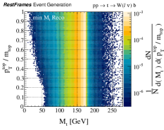
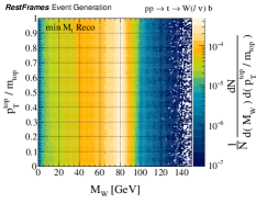
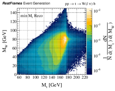
Figure 6: Distributions of (a) the W𝑊W boson mass estimator, MWsuperscriptsubscript𝑀WabsentM_{\footnotesize\mathrm{{\color[rgb]{0.45,0.0,0.09}\definecolor[named]{pgfstrokecolor}{rgb}{0.45,0.0,0.09}\textbf{\it W}}}}^{\footnotesize\leavevmode\nobreak\ }, as a function of the top mass estimator, Mtsuperscriptsubscript𝑀tabsentM_{\footnotesize\mathrm{{\color[rgb]{0.45,0.0,0.09}\definecolor[named]{pgfstrokecolor}{rgb}{0.45,0.0,0.09}\textbf{\it t}}}}^{\footnotesize\leavevmode\nobreak\ }, (b) Mtsuperscriptsubscript𝑀tabsentM_{\footnotesize\mathrm{{\color[rgb]{0.45,0.0,0.09}\definecolor[named]{pgfstrokecolor}{rgb}{0.45,0.0,0.09}\textbf{\it t}}}}^{\footnotesize\leavevmode\nobreak\ }, and (c) MWsuperscriptsubscript𝑀WabsentM_{\footnotesize\mathrm{{\color[rgb]{0.45,0.0,0.09}\definecolor[named]{pgfstrokecolor}{rgb}{0.45,0.0,0.09}\textbf{\it W}}}}^{\footnotesize\leavevmode\nobreak\ } as a function of pt,Tlab/mtsuperscriptsubscript𝑝t𝑇labsuperscriptsubscript𝑚tabsentp_{\footnotesize\mathrm{{\color[rgb]{0.45,0.0,0.09}\definecolor[named]{pgfstrokecolor}{rgb}{0.45,0.0,0.09}\textbf{\it t}}},T}^{\footnotesize\leavevmode\nobreak\ \mathrm{\textbf{lab}}}/m_{\footnotesize\mathrm{{\color[rgb]{0.45,0.0,0.09}\definecolor[named]{pgfstrokecolor}{rgb}{0.45,0.0,0.09}\textbf{\it t}}}}^{\footnotesize\leavevmode\nobreak\ }, for simulated tbW(ν)𝑡𝑏𝑊𝜈t\rightarrow bW(\ell\nu) events. The min Mtsubscript𝑀𝑡M_{t} reconstruction scheme is used for all observables.

In both reconstruction approaches, the mass estimator which is effectively minimized through the application of the invisible rapidity jigsaw corresponds to a transverse mass, with the characteristic Jacobian edges appearing at the true masses in the distributions of Fig. 5(a,b). The distribution of the observable Mtsuperscriptsubscript𝑀𝑡absentM_{\footnotesize\mathrm{{\color[rgb]{0.45,0.0,0.09}\definecolor[named]{pgfstrokecolor}{rgb}{0.45,0.0,0.09}\textbf{$t$}}}}^{\footnotesize\leavevmode\nobreak\ }, when calculated in the min MWsubscript𝑀𝑊M_{W} scheme, exhibits a more pronounced tail at high values, an undesirable feature in the context of searches looking for new particles, with potentially larger masses than their SM counterparts, and similar decays. Other observables calculated using each approach exhibit noticeable differences in behavior, such as the top and W𝑊W boson decay angles, as seen in Fig. 5(c,d). While the resolution of the reconstructed θtsubscript𝜃𝑡\theta_{\mathrm{{\color[rgb]{0.45,0.0,0.09}\definecolor[named]{pgfstrokecolor}{rgb}{0.45,0.0,0.09}\textbf{$t$}}}} is similar between the two schemes, the θtsubscript𝜃𝑡\theta_{\mathrm{{\color[rgb]{0.45,0.0,0.09}\definecolor[named]{pgfstrokecolor}{rgb}{0.45,0.0,0.09}\textbf{$t$}}}} resolution is better for the min Mtsubscript𝑀𝑡M_{t} approach, albeit with a larger bias. The improved resolution indicates that using both visible particles yields a generally more accurate estimation of pν,zlabsuperscriptsubscript𝑝𝜈𝑧labp_{\footnotesize\mathrm{{\color[rgb]{0.12,0.3,0.17}\definecolor[named]{pgfstrokecolor}{rgb}{0.12,0.3,0.17}\textbf{$\nu$}}},z}^{\footnotesize\leavevmode\nobreak\ \mathrm{\textbf{lab}}}.

When using the min Mtsubscript𝑀𝑡M_{t} strategy, the resulting Mtsuperscriptsubscript𝑀𝑡absentM_{\footnotesize\mathrm{{\color[rgb]{0.45,0.0,0.09}\definecolor[named]{pgfstrokecolor}{rgb}{0.45,0.0,0.09}\textbf{$t$}}}}^{\footnotesize\leavevmode\nobreak\ } estimator takes the form of the transverse mass of the neutrino and visible particles:

Mt 2superscriptsubscript𝑀𝑡2\displaystyle M_{\footnotesize\mathrm{{\color[rgb]{0.45,0.0,0.09}\definecolor[named]{pgfstrokecolor}{rgb}{0.45,0.0,0.09}\textbf{$t$}}}}^{\footnotesize\leavevmode\nobreak\ 2} =\displaystyle= (4)
mV 2superscriptsubscript𝑚V2\displaystyle m_{\footnotesize\mathrm{{\color[rgb]{0.1,0.1,0.44}\definecolor[named]{pgfstrokecolor}{rgb}{0.1,0.1,0.44}\textbf{V}}}}^{\footnotesize\leavevmode\nobreak\ 2} +\displaystyle+ 2(mV 2+|pV,Tlab|2|pν,Tlab|pV,Tlabpν,Tlab).2superscriptsubscript𝑚V2superscriptsuperscriptsubscript𝑝V𝑇lab2superscriptsubscript𝑝𝜈𝑇labsuperscriptsubscript𝑝V𝑇labsuperscriptsubscript𝑝𝜈𝑇lab\displaystyle 2\left(\sqrt{m_{\footnotesize\mathrm{{\color[rgb]{0.1,0.1,0.44}\definecolor[named]{pgfstrokecolor}{rgb}{0.1,0.1,0.44}\textbf{V}}}}^{\footnotesize\leavevmode\nobreak\ 2}+|\vec{p}_{\footnotesize\mathrm{{\color[rgb]{0.1,0.1,0.44}\definecolor[named]{pgfstrokecolor}{rgb}{0.1,0.1,0.44}\textbf{V}}},T}^{\footnotesize\leavevmode\nobreak\ \mathrm{\textbf{lab}}}|^{2}}|\vec{p}_{\footnotesize\mathrm{{\color[rgb]{0.12,0.3,0.17}\definecolor[named]{pgfstrokecolor}{rgb}{0.12,0.3,0.17}\textbf{$\nu$}}},T}^{\footnotesize\leavevmode\nobreak\ \mathrm{\textbf{lab}}}|-\vec{p}_{\footnotesize\mathrm{{\color[rgb]{0.1,0.1,0.44}\definecolor[named]{pgfstrokecolor}{rgb}{0.1,0.1,0.44}\textbf{V}}},T}^{\footnotesize\leavevmode\nobreak\ \mathrm{\textbf{lab}}}\cdot\vec{p}_{\footnotesize\mathrm{{\color[rgb]{0.12,0.3,0.17}\definecolor[named]{pgfstrokecolor}{rgb}{0.12,0.3,0.17}\textbf{$\nu$}}},T}^{\footnotesize\leavevmode\nobreak\ \mathrm{\textbf{lab}}}\right)\leavevmode\nobreak\ .

Since we have not chosen to minimize MWsuperscriptsubscript𝑀WabsentM_{\footnotesize\mathrm{{\color[rgb]{0.45,0.0,0.09}\definecolor[named]{pgfstrokecolor}{rgb}{0.45,0.0,0.09}\textbf{\it W}}}}^{\footnotesize\leavevmode\nobreak\ } w.r.t pν,zlabsuperscriptsubscript𝑝𝜈𝑧labp_{\footnotesize\mathrm{{\color[rgb]{0.12,0.3,0.17}\definecolor[named]{pgfstrokecolor}{rgb}{0.12,0.3,0.17}\textbf{$\nu$}}},z}^{\footnotesize\leavevmode\nobreak\ \mathrm{\textbf{lab}}}, the expression for its estimator takes a different form:

MW 2superscriptsubscript𝑀W2\displaystyle M_{\footnotesize\mathrm{{\color[rgb]{0.45,0.0,0.09}\definecolor[named]{pgfstrokecolor}{rgb}{0.45,0.0,0.09}\textbf{\it W}}}}^{\footnotesize\leavevmode\nobreak\ 2} =\displaystyle= 2(ElabEVlabp,zlabpV,zlab)|pν,Tlab|mV 2+|pV,Tlab|22superscriptsubscript𝐸labsuperscriptsubscript𝐸Vlabsuperscriptsubscript𝑝𝑧labsuperscriptsubscript𝑝V𝑧labsuperscriptsubscript𝑝𝜈𝑇labsuperscriptsubscript𝑚V2superscriptsuperscriptsubscript𝑝V𝑇lab2\displaystyle 2\left(E_{\footnotesize\mathrm{{\color[rgb]{0.1,0.1,0.44}\definecolor[named]{pgfstrokecolor}{rgb}{0.1,0.1,0.44}\textbf{$\ell$}}}}^{\footnotesize\leavevmode\nobreak\ \mathrm{\textbf{lab}}}E_{\footnotesize\mathrm{{\color[rgb]{0.1,0.1,0.44}\definecolor[named]{pgfstrokecolor}{rgb}{0.1,0.1,0.44}\textbf{V}}}}^{\footnotesize\leavevmode\nobreak\ \mathrm{\textbf{lab}}}-p_{\footnotesize\mathrm{{\color[rgb]{0.1,0.1,0.44}\definecolor[named]{pgfstrokecolor}{rgb}{0.1,0.1,0.44}\textbf{$\ell$}}},z}^{\footnotesize\leavevmode\nobreak\ \mathrm{\textbf{lab}}}p_{\footnotesize\mathrm{{\color[rgb]{0.1,0.1,0.44}\definecolor[named]{pgfstrokecolor}{rgb}{0.1,0.1,0.44}\textbf{V}}},z}^{\footnotesize\leavevmode\nobreak\ \mathrm{\textbf{lab}}}\right)\frac{|\vec{p}_{\footnotesize\mathrm{{\color[rgb]{0.12,0.3,0.17}\definecolor[named]{pgfstrokecolor}{rgb}{0.12,0.3,0.17}\textbf{$\nu$}}},T}^{\footnotesize\leavevmode\nobreak\ \mathrm{\textbf{lab}}}|}{\sqrt{m_{\footnotesize\mathrm{{\color[rgb]{0.1,0.1,0.44}\definecolor[named]{pgfstrokecolor}{rgb}{0.1,0.1,0.44}\textbf{V}}}}^{\footnotesize\leavevmode\nobreak\ 2}+|\vec{p}_{\footnotesize\mathrm{{\color[rgb]{0.1,0.1,0.44}\definecolor[named]{pgfstrokecolor}{rgb}{0.1,0.1,0.44}\textbf{V}}},T}^{\footnotesize\leavevmode\nobreak\ \mathrm{\textbf{lab}}}|^{2}}} (5)
+\displaystyle+ m 22p,Tlabpν,Tlab.superscriptsubscript𝑚22superscriptsubscript𝑝𝑇labsuperscriptsubscript𝑝𝜈𝑇lab\displaystyle m_{\footnotesize\mathrm{{\color[rgb]{0.1,0.1,0.44}\definecolor[named]{pgfstrokecolor}{rgb}{0.1,0.1,0.44}\textbf{$\ell$}}}}^{\footnotesize\leavevmode\nobreak\ 2}-2\vec{p}_{\footnotesize\mathrm{{\color[rgb]{0.1,0.1,0.44}\definecolor[named]{pgfstrokecolor}{rgb}{0.1,0.1,0.44}\textbf{$\ell$}}},T}^{\footnotesize\leavevmode\nobreak\ \mathrm{\textbf{lab}}}\cdot\vec{p}_{\footnotesize\mathrm{{\color[rgb]{0.12,0.3,0.17}\definecolor[named]{pgfstrokecolor}{rgb}{0.12,0.3,0.17}\textbf{$\nu$}}},T}^{\footnotesize\leavevmode\nobreak\ \mathrm{\textbf{lab}}}\leavevmode\nobreak\ .

This expression is longitudinally boost invariant despite using information about the lepton and b𝑏b-jet’s longitudinal momentum in the lab frame. The advantage to using a single choice for pν,zlabsuperscriptsubscript𝑝𝜈𝑧labp_{\footnotesize\mathrm{{\color[rgb]{0.12,0.3,0.17}\definecolor[named]{pgfstrokecolor}{rgb}{0.12,0.3,0.17}\textbf{$\nu$}}},z}^{\footnotesize\leavevmode\nobreak\ \mathrm{\textbf{lab}}} when calculating Mtsuperscriptsubscript𝑀tabsentM_{\footnotesize\mathrm{{\color[rgb]{0.45,0.0,0.09}\definecolor[named]{pgfstrokecolor}{rgb}{0.45,0.0,0.09}\textbf{\it t}}}}^{\footnotesize\leavevmode\nobreak\ } and MWsuperscriptsubscript𝑀WabsentM_{\footnotesize\mathrm{{\color[rgb]{0.45,0.0,0.09}\definecolor[named]{pgfstrokecolor}{rgb}{0.45,0.0,0.09}\textbf{\it W}}}}^{\footnotesize\leavevmode\nobreak\ }, rather than simply using the MWsuperscriptsubscript𝑀WabsentM_{\footnotesize\mathrm{{\color[rgb]{0.45,0.0,0.09}\definecolor[named]{pgfstrokecolor}{rgb}{0.45,0.0,0.09}\textbf{\it W}}}}^{\footnotesize\leavevmode\nobreak\ } transverse mass estimator of Eq. V.1, is that we can estimate the two masses with only small correlation, as demonstrated in Fig. 6(a). This is despite their common dependence on pν,zlabsuperscriptsubscript𝑝𝜈𝑧labp_{\footnotesize\mathrm{{\color[rgb]{0.12,0.3,0.17}\definecolor[named]{pgfstrokecolor}{rgb}{0.12,0.3,0.17}\textbf{$\nu$}}},z}^{\footnotesize\leavevmode\nobreak\ \mathrm{\textbf{lab}}}, the source of residual correlation between the observables.

While the invariance to longitudinal boosts of the Mtsuperscriptsubscript𝑀tabsentM_{\footnotesize\mathrm{{\color[rgb]{0.45,0.0,0.09}\definecolor[named]{pgfstrokecolor}{rgb}{0.45,0.0,0.09}\textbf{\it t}}}}^{\footnotesize\leavevmode\nobreak\ } and MWsuperscriptsubscript𝑀WabsentM_{\footnotesize\mathrm{{\color[rgb]{0.45,0.0,0.09}\definecolor[named]{pgfstrokecolor}{rgb}{0.45,0.0,0.09}\textbf{\it W}}}}^{\footnotesize\leavevmode\nobreak\ } observables is exact, they also exhibit little sensitivity to transverse boosts, as can be seen in Fig. 6(b,c). This behavior is indicative of the fact that observables calculated in reference frames below the lab frame in the decay tree (intermediate particle masses, decay angles) are almost entirely insensitive to the top’s velocity in the lab frame. Furthermore, the observables calculated in a particular frame are largely independent of those calculated in all other reference frames. This property makes the variables calculated in the RJR approach an excellent basis for studying processes, as it not only allows for relatively accurate estimations of many quantities of interest, but also independently.

V.3 Heavy Charged Higgs production with H+W+(ν)h0(γγ)superscript𝐻superscript𝑊𝜈superscript0𝛾𝛾\boldmath{H^{+}\rightarrow W^{+}(\ell\nu)h^{0}(\gamma\gamma)}

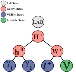
Finally, we conclude our discussion of events with a single invisible particle by adding a small embellishment to the previous example. In this case, we consider the production of a heavy, charged Higgs boson (H+superscript𝐻H^{+}) at a hadron collider, with the charged Higgs decaying to a neutral, SM-like Higgs (h0superscript0h^{0}) and a W𝑊W boson. The neutral Higgs decays to two photons, whose four vectors 𝐩γ1labsuperscriptsubscript𝐩subscript𝛾1lab\mathbf{p}_{\footnotesize\mathrm{{\color[rgb]{0.1,0.1,0.44}\definecolor[named]{pgfstrokecolor}{rgb}{0.1,0.1,0.44}\textbf{$\gamma_{1}$}}}}^{\footnotesize\leavevmode\nobreak\ \mathrm{\textbf{lab}}} and 𝐩γ2labsuperscriptsubscript𝐩subscript𝛾2lab\mathbf{p}_{\footnotesize\mathrm{{\color[rgb]{0.1,0.1,0.44}\definecolor[named]{pgfstrokecolor}{rgb}{0.1,0.1,0.44}\textbf{$\gamma_{2}$}}}}^{\footnotesize\leavevmode\nobreak\ \mathrm{\textbf{lab}}} are assumed to have been measured in the detector, while the W𝑊W decays to a lepton, with four vector 𝐩labsuperscriptsubscript𝐩lab\mathbf{p}_{\footnotesize\mathrm{{\color[rgb]{0.1,0.1,0.44}\definecolor[named]{pgfstrokecolor}{rgb}{0.1,0.1,0.44}\textbf{$\ell$}}}}^{\footnotesize\leavevmode\nobreak\ \mathrm{\textbf{lab}}}, and a neutrino, whose transverse momentum is estimated from the ETmisssuperscriptsubscript𝐸𝑇miss\vec{E}_{T}^{\rm miss}. The decay tree for interpreting this final state is shown in Fig. 7.
Refer to caption
Figure 7: A decay tree diagram of a heavy charged Higgs boson, H+superscript𝐻H^{+}, decaying to a neutral, SM-like Higgs boson, h0superscript0h^{0}, and a W𝑊W boson. The neutral Higgs decays to two photons while the W𝑊W decays to a lepton and neutrino.

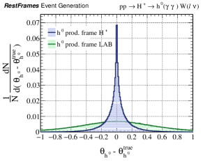
As the missing information associated with the neutrino is identical to the previous two examples, we can resolve it by choosing the neutrino mass, Mν=0superscriptsubscript𝑀𝜈absent0M_{\footnotesize\mathrm{{\color[rgb]{0.12,0.3,0.17}\definecolor[named]{pgfstrokecolor}{rgb}{0.12,0.3,0.17}\textbf{$\nu$}}}}^{\footnotesize\leavevmode\nobreak\ }=0, and applying the invisible rapidity JR V.1 using the collection of all the visible particles, V={,γ1,γ2}Vsubscript𝛾1subscript𝛾2\mathrm{{\color[rgb]{0.1,0.1,0.44}\definecolor[named]{pgfstrokecolor}{rgb}{0.1,0.1,0.44}\textbf{V}}}=\{\mathrm{{\color[rgb]{0.1,0.1,0.44}\definecolor[named]{pgfstrokecolor}{rgb}{0.1,0.1,0.44}\textbf{$\ell$}}},\mathrm{{\color[rgb]{0.1,0.1,0.44}\definecolor[named]{pgfstrokecolor}{rgb}{0.1,0.1,0.44}\textbf{$\gamma_{1}$}}},\mathrm{{\color[rgb]{0.1,0.1,0.44}\definecolor[named]{pgfstrokecolor}{rgb}{0.1,0.1,0.44}\textbf{$\gamma_{2}$}}}\}. With these choices, we are able to calculate estimators of each of the intermediate particle masses in each event, along with their decay angles. While the reconstructed neutral Higgs mass has no dependence on the neutrino kinematics, its decay angle does, as its calculation requires knowledge of the H+superscript𝐻H^{+} rest frame. The RJR approach not only allows for accurate estimation of quantities related to invisible particles, but also angles like this. Fig. 8 demonstrates the resolution that can be achieved in the estimation of this angle for simulated events, comparing the RJR observable with a calculation of cosθh0subscript𝜃superscript0\leavevmode\nobreak\ \theta_{\mathrm{{\color[rgb]{0.45,0.0,0.09}\definecolor[named]{pgfstrokecolor}{rgb}{0.45,0.0,0.09}\textbf{$h^{0}$}}}} using the lab frame as an approximation to the h0superscript0h^{0} production frame. The improvement in resolution when using the RJR approximations is dramatic.
Refer to caption
Figure 8: The decay angle of the neutral Higgs, cosθh0subscript𝜃superscript0\leavevmode\nobreak\ \theta_{\mathrm{{\color[rgb]{0.45,0.0,0.09}\definecolor[named]{pgfstrokecolor}{rgb}{0.45,0.0,0.09}\textbf{$h^{0}$}}}}, in simulated H+W+(ν)h0(γγ)superscript𝐻superscript𝑊𝜈superscript0𝛾𝛾\boldmath{H^{+}\rightarrow W^{+}(\ell\nu)h^{0}(\gamma\gamma)} events. Two different approaches to reconstructing cosθh0subscript𝜃superscript0\leavevmode\nobreak\ \theta_{\mathrm{{\color[rgb]{0.45,0.0,0.09}\definecolor[named]{pgfstrokecolor}{rgb}{0.45,0.0,0.09}\textbf{$h^{0}$}}}} are used, with one using the RJR approximation of the h0superscript0h^{0} production frame and the other treating the lab frame as that frame. Angles are shown in units radian and the mass of the charged Higgs is chosen mH+=750superscriptsubscript𝑚superscript𝐻absent750m_{\footnotesize\mathrm{{\color[rgb]{0.45,0.0,0.09}\definecolor[named]{pgfstrokecolor}{rgb}{0.45,0.0,0.09}\textbf{$H^{+}$}}}}^{\footnotesize\leavevmode\nobreak\ }=750 GeV.

VI Jigsaws for two invisible particles

To this point, we have only considered cases with a single invisible particle in the final state, and only two relevant missing pieces of information associated with its momentum and mass. When there are two invisible particles, the amount of information lost with their escape from the detector increases, as we must now guess how momentum is shared between these particles in order to approximately reconstruct events. As for Section V, we introduce new JR’s for these cases through three examples, each with increasing complexity.

VI.1 H0W+(ν)W(ν)superscript𝐻0superscript𝑊𝜈superscript𝑊𝜈H^{0}\rightarrow W^{+}(\ell\nu)W^{-}(\ell\nu) at a hadron collider

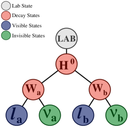
We consider an example with production of a single, neutral Higgs boson (H0superscript𝐻0H^{0}) at a hadron collider, with decays to two W𝑊W bosons which, in-turn, each decay to a lepton and neutrino. The decay tree imposed on this final state is shown in Figure 9. The two lepton four vectors, 𝐩alabsuperscriptsubscript𝐩subscript𝑎lab\mathbf{p}_{\footnotesize\mathrm{{\color[rgb]{0.1,0.1,0.44}\definecolor[named]{pgfstrokecolor}{rgb}{0.1,0.1,0.44}\textbf{$\ell_{a}$}}}}^{\footnotesize\leavevmode\nobreak\ \mathrm{\textbf{lab}}} and 𝐩blabsuperscriptsubscript𝐩subscript𝑏lab\mathbf{p}_{\footnotesize\mathrm{{\color[rgb]{0.1,0.1,0.44}\definecolor[named]{pgfstrokecolor}{rgb}{0.1,0.1,0.44}\textbf{$\ell_{b}$}}}}^{\footnotesize\leavevmode\nobreak\ \mathrm{\textbf{lab}}}, are assumed to have been measured and, working at a hadron collider, the measured ETmisssuperscriptsubscript𝐸𝑇miss\vec{E}_{T}^{\rm miss}  is interpreted as the sum transverse momentum of the two neutrinos, such that

pI,Tlab=pνa,Tlab+pνb,Tlab=ETmiss,superscriptsubscript𝑝I𝑇labsuperscriptsubscript𝑝subscript𝜈𝑎𝑇labsuperscriptsubscript𝑝subscript𝜈𝑏𝑇labsuperscriptsubscript𝐸𝑇miss\vec{p}_{\footnotesize\mathrm{{\color[rgb]{0.12,0.3,0.17}\definecolor[named]{pgfstrokecolor}{rgb}{0.12,0.3,0.17}\textbf{I}}},T}^{\footnotesize\leavevmode\nobreak\ \mathrm{\textbf{lab}}}=\vec{p}_{\footnotesize\mathrm{{\color[rgb]{0.12,0.3,0.17}\definecolor[named]{pgfstrokecolor}{rgb}{0.12,0.3,0.17}\textbf{$\nu_{a}$}}},T}^{\footnotesize\leavevmode\nobreak\ \mathrm{\textbf{lab}}}+\vec{p}_{\footnotesize\mathrm{{\color[rgb]{0.12,0.3,0.17}\definecolor[named]{pgfstrokecolor}{rgb}{0.12,0.3,0.17}\textbf{$\nu_{b}$}}},T}^{\footnotesize\leavevmode\nobreak\ \mathrm{\textbf{lab}}}=\vec{E}_{T}^{\rm miss}\leavevmode\nobreak\ , (6)

where I={νa,νb}Isubscript𝜈𝑎subscript𝜈𝑏\mathrm{{\color[rgb]{0.12,0.3,0.17}\definecolor[named]{pgfstrokecolor}{rgb}{0.12,0.3,0.17}\textbf{I}}}=\{\nu_{a},\nu_{b}\} is the set of all invisible particles in the event.
Refer to caption
Figure 9: The decay tree for analyzing H0W+(ν)W(ν)superscript𝐻0superscript𝑊𝜈superscript𝑊𝜈H^{0}\rightarrow W^{+}(\ell\nu)W^{-}(\ell\nu) events. The two sides of the event are labelled “a” and “b”, each including a lepton and neutrino from their respective W𝑊W decay.

In the previous examples with only one invisible particle in the final state we were only missing two associated pieces of information: its momentum along the beam axis and its mass. Now, with two missing particles there are only two measured constraints on the eight degrees of freedom associated with the two neutrinos’ four vectors. The total longitudinal momentum of the di-neutrino system, pI,zlabsuperscriptsubscript𝑝I𝑧labp_{\footnotesize\mathrm{{\color[rgb]{0.12,0.3,0.17}\definecolor[named]{pgfstrokecolor}{rgb}{0.12,0.3,0.17}\textbf{I}}},z}^{\footnotesize\leavevmode\nobreak\ \mathrm{\textbf{lab}}}, can be chosen using the invisible rapidity JR V.1 with the set of visible particles in the event, V={a,b}Vsubscript𝑎subscript𝑏\mathrm{{\color[rgb]{0.1,0.1,0.44}\definecolor[named]{pgfstrokecolor}{rgb}{0.1,0.1,0.44}\textbf{V}}}=\{\mathrm{{\color[rgb]{0.1,0.1,0.44}\definecolor[named]{pgfstrokecolor}{rgb}{0.1,0.1,0.44}\textbf{$\ell_{a}$}}},\mathrm{{\color[rgb]{0.1,0.1,0.44}\definecolor[named]{pgfstrokecolor}{rgb}{0.1,0.1,0.44}\textbf{$\ell_{b}$}}}\}, leaving only the mass of the neutrino system and how it is shared between the momentum of the two neutrinos to specify. We would like the JR which resolves these quantities to result in observables which, as much as possible, are independent of those we can already calculate related to the Higgs momentum in the lab frame. This is achieved by basing the determination of these additional neutrino unknowns on the four vectors of the visible leptons evaluated in the hypothetical, and yet-to-be determined, H𝐻H rest frame.

Working in this reference frame, the momentum of the I system must be equal and opposite to that of the V system, as it is the center-of-mass frame of all the final state objects. Similarly, the momentum of the W𝑊W bosons must also be equal and opposite. With only these constraints, there are many different ways to choose the unknown individual momenta of the two neutrinos. The RJR approach is to consider these unknowns as the components of the velocities relating the two W𝑊W rest frames to this H𝐻H frame, βWaHsuperscriptsubscript𝛽subscript𝑊𝑎𝐻\vec{\beta}_{\footnotesize\mathrm{{\color[rgb]{0.45,0.0,0.09}\definecolor[named]{pgfstrokecolor}{rgb}{0.45,0.0,0.09}\textbf{$W_{a}$}}}}^{\footnotesize\leavevmode\nobreak\ \mathrm{{\color[rgb]{0.45,0.0,0.09}\definecolor[named]{pgfstrokecolor}{rgb}{0.45,0.0,0.09}\textbf{$H$}}}} and βWbHsuperscriptsubscript𝛽subscript𝑊𝑏𝐻\vec{\beta}_{\footnotesize\mathrm{{\color[rgb]{0.45,0.0,0.09}\definecolor[named]{pgfstrokecolor}{rgb}{0.45,0.0,0.09}\textbf{$W_{b}$}}}}^{\footnotesize\leavevmode\nobreak\ \mathrm{{\color[rgb]{0.45,0.0,0.09}\definecolor[named]{pgfstrokecolor}{rgb}{0.45,0.0,0.09}\textbf{$H$}}}}. Ideally, we would like our derived estimators to be independent of the true values of these velocities, in a manner similar to longitudinal boost invariance through the invisible rapidity JR V.1. To achieve this, we introduce the additional constraint that the two W𝑊W bosons have the same mass. While this assumption may not be unreasonable in this particular case (although not when mH<2mWsuperscriptsubscript𝑚𝐻absent2superscriptsubscript𝑚𝑊absentm_{\footnotesize\mathrm{{\color[rgb]{0.45,0.0,0.09}\definecolor[named]{pgfstrokecolor}{rgb}{0.45,0.0,0.09}\textbf{$H$}}}}^{\footnotesize\leavevmode\nobreak\ }<2m_{\footnotesize\mathrm{{\color[rgb]{0.45,0.0,0.09}\definecolor[named]{pgfstrokecolor}{rgb}{0.45,0.0,0.09}\textbf{$W$}}}}^{\footnotesize\leavevmode\nobreak\ }, and one of the W𝑊W’s will likely be forced off-shell) this choice is primarily motivated by it allowing the two W𝑊W’s velocities to be written in terms of a single vector:

βc=βWaH=βWbH.subscript𝛽𝑐superscriptsubscript𝛽subscript𝑊𝑎𝐻superscriptsubscript𝛽subscript𝑊𝑏𝐻\vec{\beta}_{c}=\vec{\beta}_{\footnotesize\mathrm{{\color[rgb]{0.45,0.0,0.09}\definecolor[named]{pgfstrokecolor}{rgb}{0.45,0.0,0.09}\textbf{$W_{a}$}}}}^{\footnotesize\leavevmode\nobreak\ \mathrm{{\color[rgb]{0.45,0.0,0.09}\definecolor[named]{pgfstrokecolor}{rgb}{0.45,0.0,0.09}\textbf{$H$}}}}=-\vec{\beta}_{\footnotesize\mathrm{{\color[rgb]{0.45,0.0,0.09}\definecolor[named]{pgfstrokecolor}{rgb}{0.45,0.0,0.09}\textbf{$W_{b}$}}}}^{\footnotesize\leavevmode\nobreak\ \mathrm{{\color[rgb]{0.45,0.0,0.09}\definecolor[named]{pgfstrokecolor}{rgb}{0.45,0.0,0.09}\textbf{$H$}}}}\leavevmode\nobreak\ . (7)

In order to ensure that our common W𝑊W mass estimator, MWsuperscriptsubscript𝑀𝑊absentM_{\footnotesize\mathrm{{\color[rgb]{0.45,0.0,0.09}\definecolor[named]{pgfstrokecolor}{rgb}{0.45,0.0,0.09}\textbf{$W$}}}}^{\footnotesize\leavevmode\nobreak\ }, is independent of βcsubscript𝛽𝑐\vec{\beta}_{c}, we minimize it w.r.t. this unknown quantity. Neglecting the mass of the leptons and neutrinos, the dependence of MWsuperscriptsubscript𝑀𝑊absentM_{\footnotesize\mathrm{{\color[rgb]{0.45,0.0,0.09}\definecolor[named]{pgfstrokecolor}{rgb}{0.45,0.0,0.09}\textbf{$W$}}}}^{\footnotesize\leavevmode\nobreak\ } on βcsubscript𝛽𝑐\vec{\beta}_{c} can be expressed through the relation

MWsuperscriptsubscript𝑀𝑊absent\displaystyle M_{\footnotesize\mathrm{{\color[rgb]{0.45,0.0,0.09}\definecolor[named]{pgfstrokecolor}{rgb}{0.45,0.0,0.09}\textbf{$W$}}}}^{\footnotesize\leavevmode\nobreak\ } =\displaystyle= EaWa+EbWbsuperscriptsubscript𝐸subscript𝑎subscript𝑊𝑎superscriptsubscript𝐸subscript𝑏subscript𝑊𝑏\displaystyle E_{\footnotesize\mathrm{{\color[rgb]{0.1,0.1,0.44}\definecolor[named]{pgfstrokecolor}{rgb}{0.1,0.1,0.44}\textbf{$\ell_{a}$}}}}^{\footnotesize\leavevmode\nobreak\ \mathrm{{\color[rgb]{0.45,0.0,0.09}\definecolor[named]{pgfstrokecolor}{rgb}{0.45,0.0,0.09}\textbf{$W_{a}$}}}}+E_{\footnotesize\mathrm{{\color[rgb]{0.1,0.1,0.44}\definecolor[named]{pgfstrokecolor}{rgb}{0.1,0.1,0.44}\textbf{$\ell_{b}$}}}}^{\footnotesize\leavevmode\nobreak\ \mathrm{{\color[rgb]{0.45,0.0,0.09}\definecolor[named]{pgfstrokecolor}{rgb}{0.45,0.0,0.09}\textbf{$W_{b}$}}}} (8)
=\displaystyle= γc(EaH+EbHβc(paHpbH)).subscript𝛾𝑐superscriptsubscript𝐸subscript𝑎𝐻superscriptsubscript𝐸subscript𝑏𝐻subscript𝛽𝑐superscriptsubscript𝑝subscript𝑎𝐻superscriptsubscript𝑝subscript𝑏𝐻\displaystyle\gamma_{c}\left(E_{\footnotesize\mathrm{{\color[rgb]{0.1,0.1,0.44}\definecolor[named]{pgfstrokecolor}{rgb}{0.1,0.1,0.44}\textbf{$\ell_{a}$}}}}^{\footnotesize\leavevmode\nobreak\ \mathrm{{\color[rgb]{0.45,0.0,0.09}\definecolor[named]{pgfstrokecolor}{rgb}{0.45,0.0,0.09}\textbf{$H$}}}}+E_{\footnotesize\mathrm{{\color[rgb]{0.1,0.1,0.44}\definecolor[named]{pgfstrokecolor}{rgb}{0.1,0.1,0.44}\textbf{$\ell_{b}$}}}}^{\footnotesize\leavevmode\nobreak\ \mathrm{{\color[rgb]{0.45,0.0,0.09}\definecolor[named]{pgfstrokecolor}{rgb}{0.45,0.0,0.09}\textbf{$H$}}}}-\vec{\beta}_{c}\cdot(\vec{p}_{\footnotesize\mathrm{{\color[rgb]{0.1,0.1,0.44}\definecolor[named]{pgfstrokecolor}{rgb}{0.1,0.1,0.44}\textbf{$\ell_{a}$}}}}^{\footnotesize\leavevmode\nobreak\ \mathrm{{\color[rgb]{0.45,0.0,0.09}\definecolor[named]{pgfstrokecolor}{rgb}{0.45,0.0,0.09}\textbf{$H$}}}}-\vec{p}_{\footnotesize\mathrm{{\color[rgb]{0.1,0.1,0.44}\definecolor[named]{pgfstrokecolor}{rgb}{0.1,0.1,0.44}\textbf{$\ell_{b}$}}}}^{\footnotesize\leavevmode\nobreak\ \mathrm{{\color[rgb]{0.45,0.0,0.09}\definecolor[named]{pgfstrokecolor}{rgb}{0.45,0.0,0.09}\textbf{$H$}}}})\right)\leavevmode\nobreak\ .

We choose βcsubscript𝛽𝑐\vec{\beta}_{c} to satisfy

(EaWa+EbWb)βc=0,superscriptsubscript𝐸subscript𝑎subscript𝑊𝑎superscriptsubscript𝐸subscript𝑏subscript𝑊𝑏subscript𝛽𝑐0\frac{\partial\left(E_{\footnotesize\mathrm{{\color[rgb]{0.1,0.1,0.44}\definecolor[named]{pgfstrokecolor}{rgb}{0.1,0.1,0.44}\textbf{$\ell_{a}$}}}}^{\footnotesize\leavevmode\nobreak\ \mathrm{{\color[rgb]{0.45,0.0,0.09}\definecolor[named]{pgfstrokecolor}{rgb}{0.45,0.0,0.09}\textbf{$W_{a}$}}}}+E_{\footnotesize\mathrm{{\color[rgb]{0.1,0.1,0.44}\definecolor[named]{pgfstrokecolor}{rgb}{0.1,0.1,0.44}\textbf{$\ell_{b}$}}}}^{\footnotesize\leavevmode\nobreak\ \mathrm{{\color[rgb]{0.45,0.0,0.09}\definecolor[named]{pgfstrokecolor}{rgb}{0.45,0.0,0.09}\textbf{$W_{b}$}}}}\right)}{\partial\vec{\beta}_{c}}=0\leavevmode\nobreak\ , (9)

which results in

βc=paHpbHEaHEbH.subscript𝛽𝑐superscriptsubscript𝑝subscript𝑎𝐻superscriptsubscript𝑝subscript𝑏𝐻superscriptsubscript𝐸subscript𝑎𝐻superscriptsubscript𝐸subscript𝑏𝐻\vec{\beta}_{c}=\frac{\vec{p}_{\footnotesize\mathrm{{\color[rgb]{0.1,0.1,0.44}\definecolor[named]{pgfstrokecolor}{rgb}{0.1,0.1,0.44}\textbf{$\ell_{a}$}}}}^{\footnotesize\leavevmode\nobreak\ \mathrm{{\color[rgb]{0.45,0.0,0.09}\definecolor[named]{pgfstrokecolor}{rgb}{0.45,0.0,0.09}\textbf{$H$}}}}-\vec{p}_{\footnotesize\mathrm{{\color[rgb]{0.1,0.1,0.44}\definecolor[named]{pgfstrokecolor}{rgb}{0.1,0.1,0.44}\textbf{$\ell_{b}$}}}}^{\footnotesize\leavevmode\nobreak\ \mathrm{{\color[rgb]{0.45,0.0,0.09}\definecolor[named]{pgfstrokecolor}{rgb}{0.45,0.0,0.09}\textbf{$H$}}}}}{E_{\footnotesize\mathrm{{\color[rgb]{0.1,0.1,0.44}\definecolor[named]{pgfstrokecolor}{rgb}{0.1,0.1,0.44}\textbf{$\ell_{a}$}}}}^{\footnotesize\leavevmode\nobreak\ \mathrm{{\color[rgb]{0.45,0.0,0.09}\definecolor[named]{pgfstrokecolor}{rgb}{0.45,0.0,0.09}\textbf{$H$}}}}-E_{\footnotesize\mathrm{{\color[rgb]{0.1,0.1,0.44}\definecolor[named]{pgfstrokecolor}{rgb}{0.1,0.1,0.44}\textbf{$\ell_{b}$}}}}^{\footnotesize\leavevmode\nobreak\ \mathrm{{\color[rgb]{0.45,0.0,0.09}\definecolor[named]{pgfstrokecolor}{rgb}{0.45,0.0,0.09}\textbf{$H$}}}}}\leavevmode\nobreak\ . (10)

With this choice, a quantity that appears in expressions for derived estimators is the contra-boost invariant, or Euclidean mass:

Mc2(𝐩aH,𝐩bH)=2(EaHEbH+paHpbH).superscriptsubscript𝑀𝑐2superscriptsubscript𝐩subscript𝑎𝐻superscriptsubscript𝐩subscript𝑏𝐻2superscriptsubscript𝐸subscript𝑎𝐻superscriptsubscript𝐸subscript𝑏𝐻superscriptsubscript𝑝subscript𝑎𝐻superscriptsubscript𝑝subscript𝑏𝐻M_{c}^{2}(\mathbf{p}_{\footnotesize\mathrm{{\color[rgb]{0.1,0.1,0.44}\definecolor[named]{pgfstrokecolor}{rgb}{0.1,0.1,0.44}\textbf{$\ell_{a}$}}}}^{\footnotesize\leavevmode\nobreak\ \mathrm{{\color[rgb]{0.45,0.0,0.09}\definecolor[named]{pgfstrokecolor}{rgb}{0.45,0.0,0.09}\textbf{$H$}}}},\mathbf{p}_{\footnotesize\mathrm{{\color[rgb]{0.1,0.1,0.44}\definecolor[named]{pgfstrokecolor}{rgb}{0.1,0.1,0.44}\textbf{$\ell_{b}$}}}}^{\footnotesize\leavevmode\nobreak\ \mathrm{{\color[rgb]{0.45,0.0,0.09}\definecolor[named]{pgfstrokecolor}{rgb}{0.45,0.0,0.09}\textbf{$H$}}}})=2\left(E_{\footnotesize\mathrm{{\color[rgb]{0.1,0.1,0.44}\definecolor[named]{pgfstrokecolor}{rgb}{0.1,0.1,0.44}\textbf{$\ell_{a}$}}}}^{\footnotesize\leavevmode\nobreak\ \mathrm{{\color[rgb]{0.45,0.0,0.09}\definecolor[named]{pgfstrokecolor}{rgb}{0.45,0.0,0.09}\textbf{$H$}}}}E_{\footnotesize\mathrm{{\color[rgb]{0.1,0.1,0.44}\definecolor[named]{pgfstrokecolor}{rgb}{0.1,0.1,0.44}\textbf{$\ell_{b}$}}}}^{\footnotesize\leavevmode\nobreak\ \mathrm{{\color[rgb]{0.45,0.0,0.09}\definecolor[named]{pgfstrokecolor}{rgb}{0.45,0.0,0.09}\textbf{$H$}}}}+\vec{p}_{\footnotesize\mathrm{{\color[rgb]{0.1,0.1,0.44}\definecolor[named]{pgfstrokecolor}{rgb}{0.1,0.1,0.44}\textbf{$\ell_{a}$}}}}^{\footnotesize\leavevmode\nobreak\ \mathrm{{\color[rgb]{0.45,0.0,0.09}\definecolor[named]{pgfstrokecolor}{rgb}{0.45,0.0,0.09}\textbf{$H$}}}}\cdot\vec{p}_{\footnotesize\mathrm{{\color[rgb]{0.1,0.1,0.44}\definecolor[named]{pgfstrokecolor}{rgb}{0.1,0.1,0.44}\textbf{$\ell_{b}$}}}}^{\footnotesize\leavevmode\nobreak\ \mathrm{{\color[rgb]{0.45,0.0,0.09}\definecolor[named]{pgfstrokecolor}{rgb}{0.45,0.0,0.09}\textbf{$H$}}}}\right)\leavevmode\nobreak\ . (11)

Mc2superscriptsubscript𝑀𝑐2M_{c}^{2}, the inner product of two four vectors with a Euclidean metric, is unchanged under the application of any contra-boost βcsubscript𝛽𝑐\vec{\beta}_{c} such that Mc2(𝐩a,𝐩b)=Mc2(Λβc𝐩a,Λβc𝐩b)superscriptsubscript𝑀𝑐2superscriptsubscript𝐩𝑎absentsuperscriptsubscript𝐩𝑏absentsuperscriptsubscript𝑀𝑐2superscriptsubscriptΛsubscript𝛽𝑐absentsuperscriptsubscript𝐩𝑎absentsuperscriptsubscriptΛsubscript𝛽𝑐absentsuperscriptsubscript𝐩𝑏absentM_{c}^{2}(\mathbf{p}_{\footnotesize a}^{\footnotesize\leavevmode\nobreak\ },\mathbf{p}_{\footnotesize b}^{\footnotesize\leavevmode\nobreak\ })=M_{c}^{2}(\Lambda_{\footnotesize\vec{\beta}_{c}}^{\footnotesize\leavevmode\nobreak\ }\mathbf{p}_{\footnotesize a}^{\footnotesize\leavevmode\nobreak\ },\Lambda_{\footnotesize-\vec{\beta}_{c}}^{\footnotesize\leavevmode\nobreak\ }\mathbf{p}_{\footnotesize b}^{\footnotesize\leavevmode\nobreak\ }) for any two four vectors. The energy of each of the leptons, evaluated in their respective W𝑊W production frames, can be expressed as:

EiWi=mi 2+12Mc2(𝐩aH,𝐩bH)ma 2+mb 2+Mc2(𝐩aH,𝐩bH),superscriptsubscript𝐸subscript𝑖subscript𝑊𝑖superscriptsubscript𝑚subscript𝑖212superscriptsubscript𝑀𝑐2superscriptsubscript𝐩subscript𝑎𝐻superscriptsubscript𝐩subscript𝑏𝐻superscriptsubscript𝑚subscript𝑎2superscriptsubscript𝑚subscript𝑏2superscriptsubscript𝑀𝑐2superscriptsubscript𝐩subscript𝑎𝐻superscriptsubscript𝐩subscript𝑏𝐻E_{\footnotesize\mathrm{{\color[rgb]{0.1,0.1,0.44}\definecolor[named]{pgfstrokecolor}{rgb}{0.1,0.1,0.44}\textbf{$\ell_{i}$}}}}^{\footnotesize\leavevmode\nobreak\ \mathrm{{\color[rgb]{0.45,0.0,0.09}\definecolor[named]{pgfstrokecolor}{rgb}{0.45,0.0,0.09}\textbf{$W_{i}$}}}}=\frac{m_{\footnotesize\mathrm{{\color[rgb]{0.1,0.1,0.44}\definecolor[named]{pgfstrokecolor}{rgb}{0.1,0.1,0.44}\textbf{$\ell_{i}$}}}}^{\footnotesize\leavevmode\nobreak\ 2}+\frac{1}{2}M_{c}^{2}(\mathbf{p}_{\footnotesize\mathrm{{\color[rgb]{0.1,0.1,0.44}\definecolor[named]{pgfstrokecolor}{rgb}{0.1,0.1,0.44}\textbf{$\ell_{a}$}}}}^{\footnotesize\leavevmode\nobreak\ \mathrm{{\color[rgb]{0.45,0.0,0.09}\definecolor[named]{pgfstrokecolor}{rgb}{0.45,0.0,0.09}\textbf{$H$}}}},\mathbf{p}_{\footnotesize\mathrm{{\color[rgb]{0.1,0.1,0.44}\definecolor[named]{pgfstrokecolor}{rgb}{0.1,0.1,0.44}\textbf{$\ell_{b}$}}}}^{\footnotesize\leavevmode\nobreak\ \mathrm{{\color[rgb]{0.45,0.0,0.09}\definecolor[named]{pgfstrokecolor}{rgb}{0.45,0.0,0.09}\textbf{$H$}}}})}{\sqrt{m_{\footnotesize\mathrm{{\color[rgb]{0.1,0.1,0.44}\definecolor[named]{pgfstrokecolor}{rgb}{0.1,0.1,0.44}\textbf{$\ell_{a}$}}}}^{\footnotesize\leavevmode\nobreak\ 2}+m_{\footnotesize\mathrm{{\color[rgb]{0.1,0.1,0.44}\definecolor[named]{pgfstrokecolor}{rgb}{0.1,0.1,0.44}\textbf{$\ell_{b}$}}}}^{\footnotesize\leavevmode\nobreak\ 2}+M_{c}^{2}(\mathbf{p}_{\footnotesize\mathrm{{\color[rgb]{0.1,0.1,0.44}\definecolor[named]{pgfstrokecolor}{rgb}{0.1,0.1,0.44}\textbf{$\ell_{a}$}}}}^{\footnotesize\leavevmode\nobreak\ \mathrm{{\color[rgb]{0.45,0.0,0.09}\definecolor[named]{pgfstrokecolor}{rgb}{0.45,0.0,0.09}\textbf{$H$}}}},\mathbf{p}_{\footnotesize\mathrm{{\color[rgb]{0.1,0.1,0.44}\definecolor[named]{pgfstrokecolor}{rgb}{0.1,0.1,0.44}\textbf{$\ell_{b}$}}}}^{\footnotesize\leavevmode\nobreak\ \mathrm{{\color[rgb]{0.45,0.0,0.09}\definecolor[named]{pgfstrokecolor}{rgb}{0.45,0.0,0.09}\textbf{$H$}}}})}}\leavevmode\nobreak\ , (12)

which is manifestly contra-boost invariant, as desired.

After choosing βcsubscript𝛽𝑐\vec{\beta}_{c}, there is still one unspecified degree of freedom associated with the individual neutrino, and di-neutrino, masses. Expressing this remaining parameter as c𝑐c, we can write

Mνa 2superscriptsubscript𝑀subscript𝜈𝑎2\displaystyle M_{\footnotesize\mathrm{{\color[rgb]{0.12,0.3,0.17}\definecolor[named]{pgfstrokecolor}{rgb}{0.12,0.3,0.17}\textbf{$\nu_{a}$}}}}^{\footnotesize\leavevmode\nobreak\ 2} =\displaystyle= (c1)2ma 2+c2mb 2+(c1)cMc2(𝐩aH,𝐩bH)superscript𝑐12superscriptsubscript𝑚subscript𝑎2superscript𝑐2superscriptsubscript𝑚subscript𝑏2𝑐1𝑐superscriptsubscript𝑀𝑐2superscriptsubscript𝐩subscript𝑎𝐻superscriptsubscript𝐩subscript𝑏𝐻\displaystyle(c-1)^{2}m_{\footnotesize\mathrm{{\color[rgb]{0.1,0.1,0.44}\definecolor[named]{pgfstrokecolor}{rgb}{0.1,0.1,0.44}\textbf{$\ell_{a}$}}}}^{\footnotesize\leavevmode\nobreak\ 2}+c^{2}m_{\footnotesize\mathrm{{\color[rgb]{0.1,0.1,0.44}\definecolor[named]{pgfstrokecolor}{rgb}{0.1,0.1,0.44}\textbf{$\ell_{b}$}}}}^{\footnotesize\leavevmode\nobreak\ 2}+(c-1)cM_{c}^{2}(\mathbf{p}_{\footnotesize\mathrm{{\color[rgb]{0.1,0.1,0.44}\definecolor[named]{pgfstrokecolor}{rgb}{0.1,0.1,0.44}\textbf{$\ell_{a}$}}}}^{\footnotesize\leavevmode\nobreak\ \mathrm{{\color[rgb]{0.45,0.0,0.09}\definecolor[named]{pgfstrokecolor}{rgb}{0.45,0.0,0.09}\textbf{$H$}}}},\mathbf{p}_{\footnotesize\mathrm{{\color[rgb]{0.1,0.1,0.44}\definecolor[named]{pgfstrokecolor}{rgb}{0.1,0.1,0.44}\textbf{$\ell_{b}$}}}}^{\footnotesize\leavevmode\nobreak\ \mathrm{{\color[rgb]{0.45,0.0,0.09}\definecolor[named]{pgfstrokecolor}{rgb}{0.45,0.0,0.09}\textbf{$H$}}}})
Mνb 2superscriptsubscript𝑀subscript𝜈𝑏2\displaystyle M_{\footnotesize\mathrm{{\color[rgb]{0.12,0.3,0.17}\definecolor[named]{pgfstrokecolor}{rgb}{0.12,0.3,0.17}\textbf{$\nu_{b}$}}}}^{\footnotesize\leavevmode\nobreak\ 2} =\displaystyle= (c1)2mb 2+c2ma 2+(c1)cMc2(𝐩aH,𝐩bH)superscript𝑐12superscriptsubscript𝑚subscript𝑏2superscript𝑐2superscriptsubscript𝑚subscript𝑎2𝑐1𝑐superscriptsubscript𝑀𝑐2superscriptsubscript𝐩subscript𝑎𝐻superscriptsubscript𝐩subscript𝑏𝐻\displaystyle(c-1)^{2}m_{\footnotesize\mathrm{{\color[rgb]{0.1,0.1,0.44}\definecolor[named]{pgfstrokecolor}{rgb}{0.1,0.1,0.44}\textbf{$\ell_{b}$}}}}^{\footnotesize\leavevmode\nobreak\ 2}+c^{2}m_{\footnotesize\mathrm{{\color[rgb]{0.1,0.1,0.44}\definecolor[named]{pgfstrokecolor}{rgb}{0.1,0.1,0.44}\textbf{$\ell_{a}$}}}}^{\footnotesize\leavevmode\nobreak\ 2}+(c-1)cM_{c}^{2}(\mathbf{p}_{\footnotesize\mathrm{{\color[rgb]{0.1,0.1,0.44}\definecolor[named]{pgfstrokecolor}{rgb}{0.1,0.1,0.44}\textbf{$\ell_{a}$}}}}^{\footnotesize\leavevmode\nobreak\ \mathrm{{\color[rgb]{0.45,0.0,0.09}\definecolor[named]{pgfstrokecolor}{rgb}{0.45,0.0,0.09}\textbf{$H$}}}},\mathbf{p}_{\footnotesize\mathrm{{\color[rgb]{0.1,0.1,0.44}\definecolor[named]{pgfstrokecolor}{rgb}{0.1,0.1,0.44}\textbf{$\ell_{b}$}}}}^{\footnotesize\leavevmode\nobreak\ \mathrm{{\color[rgb]{0.45,0.0,0.09}\definecolor[named]{pgfstrokecolor}{rgb}{0.45,0.0,0.09}\textbf{$H$}}}})
MI 2superscriptsubscript𝑀I2\displaystyle M_{\footnotesize\mathrm{{\color[rgb]{0.12,0.3,0.17}\definecolor[named]{pgfstrokecolor}{rgb}{0.12,0.3,0.17}\textbf{I}}}}^{\footnotesize\leavevmode\nobreak\ 2} =\displaystyle= (2c1)2(EVH)2|pVH|2.superscript2𝑐12superscriptsuperscriptsubscript𝐸V𝐻2superscriptsuperscriptsubscript𝑝V𝐻2\displaystyle(2c-1)^{2}(E_{\footnotesize\mathrm{{\color[rgb]{0.1,0.1,0.44}\definecolor[named]{pgfstrokecolor}{rgb}{0.1,0.1,0.44}\textbf{V}}}}^{\footnotesize\leavevmode\nobreak\ \mathrm{{\color[rgb]{0.45,0.0,0.09}\definecolor[named]{pgfstrokecolor}{rgb}{0.45,0.0,0.09}\textbf{$H$}}}})^{2}-|\vec{p}_{\footnotesize\mathrm{{\color[rgb]{0.1,0.1,0.44}\definecolor[named]{pgfstrokecolor}{rgb}{0.1,0.1,0.44}\textbf{V}}}}^{\footnotesize\leavevmode\nobreak\ \mathrm{{\color[rgb]{0.45,0.0,0.09}\definecolor[named]{pgfstrokecolor}{rgb}{0.45,0.0,0.09}\textbf{$H$}}}}|^{2}\leavevmode\nobreak\ . (13)

where different values of c𝑐c are seen to increase and decrease each of the neutrino-related masses coherently. Neglecting the individual lepton masses, a choice of c=1𝑐1c=1 sets the neutrino masses to zero, and also implies MI=mVsuperscriptsubscript𝑀Iabsentsuperscriptsubscript𝑚VabsentM_{\footnotesize\mathrm{{\color[rgb]{0.12,0.3,0.17}\definecolor[named]{pgfstrokecolor}{rgb}{0.12,0.3,0.17}\textbf{I}}}}^{\footnotesize\leavevmode\nobreak\ }=m_{\footnotesize\mathrm{{\color[rgb]{0.1,0.1,0.44}\definecolor[named]{pgfstrokecolor}{rgb}{0.1,0.1,0.44}\textbf{V}}}}^{\footnotesize\leavevmode\nobreak\ }. From Eq. VI.1 we also observe that a smaller choice for c𝑐c (or, alternatively, smaller choice for MIsuperscriptsubscript𝑀IabsentM_{\footnotesize\mathrm{{\color[rgb]{0.12,0.3,0.17}\definecolor[named]{pgfstrokecolor}{rgb}{0.12,0.3,0.17}\textbf{I}}}}^{\footnotesize\leavevmode\nobreak\ }) could lead to tachyonic individual neutrinos. This means that while a choice of MIsuperscriptsubscript𝑀IabsentM_{\footnotesize\mathrm{{\color[rgb]{0.12,0.3,0.17}\definecolor[named]{pgfstrokecolor}{rgb}{0.12,0.3,0.17}\textbf{I}}}}^{\footnotesize\leavevmode\nobreak\ } larger than mVsuperscriptsubscript𝑚Vabsentm_{\footnotesize\mathrm{{\color[rgb]{0.1,0.1,0.44}\definecolor[named]{pgfstrokecolor}{rgb}{0.1,0.1,0.44}\textbf{V}}}}^{\footnotesize\leavevmode\nobreak\ } would be consistent with the above prescription, smaller choices are not sufficiently large to use this approach. As the calculation of the velocity relating the lab frame to the H𝐻H rest frame depends on MIsuperscriptsubscript𝑀IabsentM_{\footnotesize\mathrm{{\color[rgb]{0.12,0.3,0.17}\definecolor[named]{pgfstrokecolor}{rgb}{0.12,0.3,0.17}\textbf{I}}}}^{\footnotesize\leavevmode\nobreak\ }, in the RJR scheme this choice must be made appealing only to the four vectors of visible particles in the lab frame. Fortunately, the minimum value necessary to ensure our ultimate neutrino approximations are physically viable, mVsuperscriptsubscript𝑚Vabsentm_{\footnotesize\mathrm{{\color[rgb]{0.1,0.1,0.44}\definecolor[named]{pgfstrokecolor}{rgb}{0.1,0.1,0.44}\textbf{V}}}}^{\footnotesize\leavevmode\nobreak\ }, is a Lorentz-invariant function of these four vectors, meaning we can make this assignment only knowing our prescription for analyzing the event in the H𝐻H rest frame, but not necessarily having enough information to evaluate any visible four vectors there. This choice corresponds to a JR:

Jigsaw Rule VI.1 (Invisible Mass)

If the mass of an invisible particle, I, is unknown it can be chosen to be the smallest Lorentz invariant function of visible four vectors that is sufficiently large to accommodate any other applied JR’s which correspond to dividing I into other invisible particles.

Similarly, the above prescription for choosing βcsubscript𝛽𝑐\vec{\beta}_{c} can be generalized as another JR:

Jigsaw Rule VI.2 (Contra-boost Invariant)

If the internal degrees of freedom specifying how an invisible particle, I={Ia,Ib}IIaIb\mathrm{{\color[rgb]{0.12,0.3,0.17}\definecolor[named]{pgfstrokecolor}{rgb}{0.12,0.3,0.17}\textbf{I}}}=\{\mathrm{{\color[rgb]{0.12,0.3,0.17}\definecolor[named]{pgfstrokecolor}{rgb}{0.12,0.3,0.17}\textbf{I${}_{a}$}}},\mathrm{{\color[rgb]{0.12,0.3,0.17}\definecolor[named]{pgfstrokecolor}{rgb}{0.12,0.3,0.17}\textbf{I${}_{b}$}}}\}, should split into two particles are unknown, they can be specified by choosing a corresponding pair of visible particles, V={Va,Vb}VVaVb\mathrm{{\color[rgb]{0.1,0.1,0.44}\definecolor[named]{pgfstrokecolor}{rgb}{0.1,0.1,0.44}\textbf{V}}}=\{\mathrm{{\color[rgb]{0.1,0.1,0.44}\definecolor[named]{pgfstrokecolor}{rgb}{0.1,0.1,0.44}\textbf{V${}_{a}$}}},\mathrm{{\color[rgb]{0.1,0.1,0.44}\definecolor[named]{pgfstrokecolor}{rgb}{0.1,0.1,0.44}\textbf{V${}_{b}$}}}\}, and applying the constraint MVaIa=MVbIbsuperscriptsubscript𝑀VaIaabsentsuperscriptsubscript𝑀VbIbabsentM_{\footnotesize\mathrm{{\color[rgb]{0.1,0.1,0.44}\definecolor[named]{pgfstrokecolor}{rgb}{0.1,0.1,0.44}\textbf{V${}_{a}$}}}\mathrm{{\color[rgb]{0.12,0.3,0.17}\definecolor[named]{pgfstrokecolor}{rgb}{0.12,0.3,0.17}\textbf{I${}_{a}$}}}}^{\footnotesize\leavevmode\nobreak\ }=M_{\footnotesize\mathrm{{\color[rgb]{0.1,0.1,0.44}\definecolor[named]{pgfstrokecolor}{rgb}{0.1,0.1,0.44}\textbf{V${}_{b}$}}}\mathrm{{\color[rgb]{0.12,0.3,0.17}\definecolor[named]{pgfstrokecolor}{rgb}{0.12,0.3,0.17}\textbf{I${}_{b}$}}}}^{\footnotesize\leavevmode\nobreak\ }. It is assumed that the four vectors of the visible particles are known in the center-of-mass frame, F={V,I}FVI\mathrm{{\color[rgb]{0.45,0.0,0.09}\definecolor[named]{pgfstrokecolor}{rgb}{0.45,0.0,0.09}\textbf{F}}}=\{\mathrm{{\color[rgb]{0.1,0.1,0.44}\definecolor[named]{pgfstrokecolor}{rgb}{0.1,0.1,0.44}\textbf{V}}},\mathrm{{\color[rgb]{0.12,0.3,0.17}\definecolor[named]{pgfstrokecolor}{rgb}{0.12,0.3,0.17}\textbf{I}}}\leavevmode\nobreak\ \}, as is the four vector of the total I system, 𝐩IFsuperscriptsubscript𝐩IF\mathbf{p}_{\footnotesize\mathrm{{\color[rgb]{0.12,0.3,0.17}\definecolor[named]{pgfstrokecolor}{rgb}{0.12,0.3,0.17}\textbf{I}}}}^{\footnotesize\leavevmode\nobreak\ \mathrm{{\color[rgb]{0.45,0.0,0.09}\definecolor[named]{pgfstrokecolor}{rgb}{0.45,0.0,0.09}\textbf{F}}}}. The four vectors of the invisible particles can be chosen in the F frame as:

pIaFsuperscriptsubscript𝑝IaF\displaystyle\vec{p}_{\footnotesize\mathrm{{\color[rgb]{0.12,0.3,0.17}\definecolor[named]{pgfstrokecolor}{rgb}{0.12,0.3,0.17}\textbf{I${}_{a}$}}}}^{\footnotesize\leavevmode\nobreak\ \mathrm{{\color[rgb]{0.45,0.0,0.09}\definecolor[named]{pgfstrokecolor}{rgb}{0.45,0.0,0.09}\textbf{F}}}} =\displaystyle= (c1)pVaFcpVbF𝑐1superscriptsubscript𝑝VaF𝑐superscriptsubscript𝑝VbF\displaystyle(c-1)\vec{p}_{\footnotesize\mathrm{{\color[rgb]{0.1,0.1,0.44}\definecolor[named]{pgfstrokecolor}{rgb}{0.1,0.1,0.44}\textbf{V${}_{a}$}}}}^{\footnotesize\leavevmode\nobreak\ \mathrm{{\color[rgb]{0.45,0.0,0.09}\definecolor[named]{pgfstrokecolor}{rgb}{0.45,0.0,0.09}\textbf{F}}}}-c\vec{p}_{\footnotesize\mathrm{{\color[rgb]{0.1,0.1,0.44}\definecolor[named]{pgfstrokecolor}{rgb}{0.1,0.1,0.44}\textbf{V${}_{b}$}}}}^{\footnotesize\leavevmode\nobreak\ \mathrm{{\color[rgb]{0.45,0.0,0.09}\definecolor[named]{pgfstrokecolor}{rgb}{0.45,0.0,0.09}\textbf{F}}}}
pIbFsuperscriptsubscript𝑝IbF\displaystyle\vec{p}_{\footnotesize\mathrm{{\color[rgb]{0.12,0.3,0.17}\definecolor[named]{pgfstrokecolor}{rgb}{0.12,0.3,0.17}\textbf{I${}_{b}$}}}}^{\footnotesize\leavevmode\nobreak\ \mathrm{{\color[rgb]{0.45,0.0,0.09}\definecolor[named]{pgfstrokecolor}{rgb}{0.45,0.0,0.09}\textbf{F}}}} =\displaystyle= (c1)pVbFcpVaF𝑐1superscriptsubscript𝑝VbF𝑐superscriptsubscript𝑝VaF\displaystyle(c-1)\vec{p}_{\footnotesize\mathrm{{\color[rgb]{0.1,0.1,0.44}\definecolor[named]{pgfstrokecolor}{rgb}{0.1,0.1,0.44}\textbf{V${}_{b}$}}}}^{\footnotesize\leavevmode\nobreak\ \mathrm{{\color[rgb]{0.45,0.0,0.09}\definecolor[named]{pgfstrokecolor}{rgb}{0.45,0.0,0.09}\textbf{F}}}}-c\vec{p}_{\footnotesize\mathrm{{\color[rgb]{0.1,0.1,0.44}\definecolor[named]{pgfstrokecolor}{rgb}{0.1,0.1,0.44}\textbf{V${}_{a}$}}}}^{\footnotesize\leavevmode\nobreak\ \mathrm{{\color[rgb]{0.45,0.0,0.09}\definecolor[named]{pgfstrokecolor}{rgb}{0.45,0.0,0.09}\textbf{F}}}} (14)
EIaFsuperscriptsubscript𝐸IaF\displaystyle E_{\footnotesize\mathrm{{\color[rgb]{0.12,0.3,0.17}\definecolor[named]{pgfstrokecolor}{rgb}{0.12,0.3,0.17}\textbf{I${}_{a}$}}}}^{\footnotesize\leavevmode\nobreak\ \mathrm{{\color[rgb]{0.45,0.0,0.09}\definecolor[named]{pgfstrokecolor}{rgb}{0.45,0.0,0.09}\textbf{F}}}} =\displaystyle= (c1)EVaF+cEVbF𝑐1superscriptsubscript𝐸VaF𝑐superscriptsubscript𝐸VbF\displaystyle(c-1)E_{\footnotesize\mathrm{{\color[rgb]{0.1,0.1,0.44}\definecolor[named]{pgfstrokecolor}{rgb}{0.1,0.1,0.44}\textbf{V${}_{a}$}}}}^{\footnotesize\leavevmode\nobreak\ \mathrm{{\color[rgb]{0.45,0.0,0.09}\definecolor[named]{pgfstrokecolor}{rgb}{0.45,0.0,0.09}\textbf{F}}}}+cE_{\footnotesize\mathrm{{\color[rgb]{0.1,0.1,0.44}\definecolor[named]{pgfstrokecolor}{rgb}{0.1,0.1,0.44}\textbf{V${}_{b}$}}}}^{\footnotesize\leavevmode\nobreak\ \mathrm{{\color[rgb]{0.45,0.0,0.09}\definecolor[named]{pgfstrokecolor}{rgb}{0.45,0.0,0.09}\textbf{F}}}}
EIbFsuperscriptsubscript𝐸IbF\displaystyle E_{\footnotesize\mathrm{{\color[rgb]{0.12,0.3,0.17}\definecolor[named]{pgfstrokecolor}{rgb}{0.12,0.3,0.17}\textbf{I${}_{b}$}}}}^{\footnotesize\leavevmode\nobreak\ \mathrm{{\color[rgb]{0.45,0.0,0.09}\definecolor[named]{pgfstrokecolor}{rgb}{0.45,0.0,0.09}\textbf{F}}}} =\displaystyle= (c1)EVbF+cEVaF,𝑐1superscriptsubscript𝐸VbF𝑐superscriptsubscript𝐸VaF\displaystyle(c-1)E_{\footnotesize\mathrm{{\color[rgb]{0.1,0.1,0.44}\definecolor[named]{pgfstrokecolor}{rgb}{0.1,0.1,0.44}\textbf{V${}_{b}$}}}}^{\footnotesize\leavevmode\nobreak\ \mathrm{{\color[rgb]{0.45,0.0,0.09}\definecolor[named]{pgfstrokecolor}{rgb}{0.45,0.0,0.09}\textbf{F}}}}+cE_{\footnotesize\mathrm{{\color[rgb]{0.1,0.1,0.44}\definecolor[named]{pgfstrokecolor}{rgb}{0.1,0.1,0.44}\textbf{V${}_{a}$}}}}^{\footnotesize\leavevmode\nobreak\ \mathrm{{\color[rgb]{0.45,0.0,0.09}\definecolor[named]{pgfstrokecolor}{rgb}{0.45,0.0,0.09}\textbf{F}}}}\leavevmode\nobreak\ ,

where

c=12[1+(EVF)2mV 2+MI 2EVF].𝑐12delimited-[]1superscriptsuperscriptsubscript𝐸VF2superscriptsubscript𝑚V2superscriptsubscript𝑀I2superscriptsubscript𝐸VF\displaystyle c=\frac{1}{2}\left[1+\frac{\sqrt{(E_{\footnotesize\mathrm{{\color[rgb]{0.1,0.1,0.44}\definecolor[named]{pgfstrokecolor}{rgb}{0.1,0.1,0.44}\textbf{V}}}}^{\footnotesize\leavevmode\nobreak\ \mathrm{{\color[rgb]{0.45,0.0,0.09}\definecolor[named]{pgfstrokecolor}{rgb}{0.45,0.0,0.09}\textbf{F}}}})^{2}-m_{\footnotesize\mathrm{{\color[rgb]{0.1,0.1,0.44}\definecolor[named]{pgfstrokecolor}{rgb}{0.1,0.1,0.44}\textbf{V}}}}^{\footnotesize\leavevmode\nobreak\ 2}+M_{\footnotesize\mathrm{{\color[rgb]{0.12,0.3,0.17}\definecolor[named]{pgfstrokecolor}{rgb}{0.12,0.3,0.17}\textbf{I}}}}^{\footnotesize\leavevmode\nobreak\ 2}}}{E_{\footnotesize\mathrm{{\color[rgb]{0.1,0.1,0.44}\definecolor[named]{pgfstrokecolor}{rgb}{0.1,0.1,0.44}\textbf{V}}}}^{\footnotesize\leavevmode\nobreak\ \mathrm{{\color[rgb]{0.45,0.0,0.09}\definecolor[named]{pgfstrokecolor}{rgb}{0.45,0.0,0.09}\textbf{F}}}}}\right]\leavevmode\nobreak\ . (15)

If the visible particles Va and Vb are massless, the minimum value of MIsuperscriptsubscript𝑀IabsentM_{\footnotesize\mathrm{{\color[rgb]{0.12,0.3,0.17}\definecolor[named]{pgfstrokecolor}{rgb}{0.12,0.3,0.17}\textbf{I}}}}^{\footnotesize\leavevmode\nobreak\ } required to guarantee that the individual invisible particles will not be tachyonic is mVsuperscriptsubscript𝑚Vabsentm_{\footnotesize\mathrm{{\color[rgb]{0.1,0.1,0.44}\definecolor[named]{pgfstrokecolor}{rgb}{0.1,0.1,0.44}\textbf{V}}}}^{\footnotesize\leavevmode\nobreak\ }.

With these JR’s defined, we can summarize the RJR approach for analyzing H0W+(+ν)W(ν)superscript𝐻0superscript𝑊superscript𝜈superscript𝑊superscript𝜈H^{0}\rightarrow W^{+}(\ell^{+}\nu)W^{-}(\ell^{-}\nu) events:

  1. 1.

    Apply the invisible mass JR VI.1,
    choosing MI=mVsuperscriptsubscript𝑀Iabsentsuperscriptsubscript𝑚VabsentM_{\footnotesize\mathrm{{\color[rgb]{0.12,0.3,0.17}\definecolor[named]{pgfstrokecolor}{rgb}{0.12,0.3,0.17}\textbf{I}}}}^{\footnotesize\leavevmode\nobreak\ }=m_{\footnotesize\mathrm{{\color[rgb]{0.1,0.1,0.44}\definecolor[named]{pgfstrokecolor}{rgb}{0.1,0.1,0.44}\textbf{V}}}}^{\footnotesize\leavevmode\nobreak\ }

  2. 2.

    Apply the invisible rapidity JR V.1,
    choosing pI,zlabsuperscriptsubscript𝑝I𝑧labp_{\footnotesize\mathrm{{\color[rgb]{0.12,0.3,0.17}\definecolor[named]{pgfstrokecolor}{rgb}{0.12,0.3,0.17}\textbf{I}}},z}^{\footnotesize\leavevmode\nobreak\ \mathrm{\textbf{lab}}} using the leptons V

  3. 3.

    Apply the contra-boost invariant JR VI.2,
    specifying the neutrino four vectors
    using the constraint MWa=MWbsuperscriptsubscript𝑀subscript𝑊𝑎absentsuperscriptsubscript𝑀subscript𝑊𝑏absentM_{\footnotesize\mathrm{{\color[rgb]{0.45,0.0,0.09}\definecolor[named]{pgfstrokecolor}{rgb}{0.45,0.0,0.09}\textbf{$W_{a}$}}}}^{\footnotesize\leavevmode\nobreak\ }=M_{\footnotesize\mathrm{{\color[rgb]{0.45,0.0,0.09}\definecolor[named]{pgfstrokecolor}{rgb}{0.45,0.0,0.09}\textbf{$W_{b}$}}}}^{\footnotesize\leavevmode\nobreak\ }

After the application of these JR’s, values for all of the unknowns in the event are specified and any kinematic quantity of interest can be estimated.

One natural quantity of interest is the mass of the heavy, neutral Higgs, shown in Fig. 10 for different values of mHsuperscriptsubscript𝑚𝐻absentm_{\footnotesize\mathrm{{\color[rgb]{0.45,0.0,0.09}\definecolor[named]{pgfstrokecolor}{rgb}{0.45,0.0,0.09}\textbf{$H$}}}}^{\footnotesize\leavevmode\nobreak\ }. The relative resolution of the Higgs mass estimator, MHsuperscriptsubscript𝑀𝐻absentM_{\footnotesize\mathrm{{\color[rgb]{0.45,0.0,0.09}\definecolor[named]{pgfstrokecolor}{rgb}{0.45,0.0,0.09}\textbf{$H$}}}}^{\footnotesize\leavevmode\nobreak\ }, is approximately the same for mH>2mWsuperscriptsubscript𝑚𝐻absent2subscript𝑚𝑊m_{\footnotesize\mathrm{{\color[rgb]{0.45,0.0,0.09}\definecolor[named]{pgfstrokecolor}{rgb}{0.45,0.0,0.09}\textbf{$H$}}}}^{\footnotesize\leavevmode\nobreak\ }>2m_{W}, with the peak of each distribution scaling with the true value, and a slight underestimation visible due to the implicit minimization in the invisible rapidity JR.
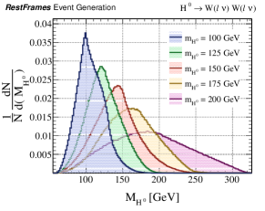
Refer to caption
Figure 10: Distribution of MHsuperscriptsubscript𝑀𝐻absentM_{\footnotesize\mathrm{{\color[rgb]{0.45,0.0,0.09}\definecolor[named]{pgfstrokecolor}{rgb}{0.45,0.0,0.09}\textbf{$H$}}}}^{\footnotesize\leavevmode\nobreak\ } for simulated H0W+(ν)W(ν)superscript𝐻0superscript𝑊𝜈superscript𝑊𝜈H^{0}\rightarrow W^{+}(\ell\nu)W^{-}(\ell\nu) events with various values for mHsuperscriptsubscript𝑚𝐻absentm_{\footnotesize\mathrm{{\color[rgb]{0.45,0.0,0.09}\definecolor[named]{pgfstrokecolor}{rgb}{0.45,0.0,0.09}\textbf{$H$}}}}^{\footnotesize\leavevmode\nobreak\ }.

Like MHsuperscriptsubscript𝑀𝐻absentM_{\footnotesize\mathrm{{\color[rgb]{0.45,0.0,0.09}\definecolor[named]{pgfstrokecolor}{rgb}{0.45,0.0,0.09}\textbf{$H$}}}}^{\footnotesize\leavevmode\nobreak\ }, the W𝑊W mass estimator, MWsuperscriptsubscript𝑀𝑊absentM_{\footnotesize\mathrm{{\color[rgb]{0.45,0.0,0.09}\definecolor[named]{pgfstrokecolor}{rgb}{0.45,0.0,0.09}\textbf{$W$}}}}^{\footnotesize\leavevmode\nobreak\ }, also provides sensitivity to the true value, exhibiting a kinematic edge as can be observed in Fig. 11. The shape of the MWsuperscriptsubscript𝑀𝑊absentM_{\footnotesize\mathrm{{\color[rgb]{0.45,0.0,0.09}\definecolor[named]{pgfstrokecolor}{rgb}{0.45,0.0,0.09}\textbf{$W$}}}}^{\footnotesize\leavevmode\nobreak\ } distribution is largely independent of the value of mHsuperscriptsubscript𝑚𝐻absentm_{\footnotesize\mathrm{{\color[rgb]{0.45,0.0,0.09}\definecolor[named]{pgfstrokecolor}{rgb}{0.45,0.0,0.09}\textbf{$H$}}}}^{\footnotesize\leavevmode\nobreak\ }, and event-by-event it is estimated largely independently of MHsuperscriptsubscript𝑀𝐻absentM_{\footnotesize\mathrm{{\color[rgb]{0.45,0.0,0.09}\definecolor[named]{pgfstrokecolor}{rgb}{0.45,0.0,0.09}\textbf{$H$}}}}^{\footnotesize\leavevmode\nobreak\ }, with the resolution of MHsuperscriptsubscript𝑀𝐻absentM_{\footnotesize\mathrm{{\color[rgb]{0.45,0.0,0.09}\definecolor[named]{pgfstrokecolor}{rgb}{0.45,0.0,0.09}\textbf{$H$}}}}^{\footnotesize\leavevmode\nobreak\ } correlated with how close MWsuperscriptsubscript𝑀𝑊absentM_{\footnotesize\mathrm{{\color[rgb]{0.45,0.0,0.09}\definecolor[named]{pgfstrokecolor}{rgb}{0.45,0.0,0.09}\textbf{$W$}}}}^{\footnotesize\leavevmode\nobreak\ } is to its approximate kinematic boundary. This lack of correlation is a result of the JR rules applied. The contra-boost invariant JR ensures that MWsuperscriptsubscript𝑀𝑊absentM_{\footnotesize\mathrm{{\color[rgb]{0.45,0.0,0.09}\definecolor[named]{pgfstrokecolor}{rgb}{0.45,0.0,0.09}\textbf{$W$}}}}^{\footnotesize\leavevmode\nobreak\ } is largely insensitive to the W𝑊W boson velocity in its production frame, which is roughly proportional to the mass of H𝐻H.

Refer to caption
Figure 11: Distribution of MWsuperscriptsubscript𝑀𝑊absentM_{\footnotesize\mathrm{{\color[rgb]{0.45,0.0,0.09}\definecolor[named]{pgfstrokecolor}{rgb}{0.45,0.0,0.09}\textbf{$W$}}}}^{\footnotesize\leavevmode\nobreak\ }, as a function of MHsuperscriptsubscript𝑀𝐻absentM_{\footnotesize\mathrm{{\color[rgb]{0.45,0.0,0.09}\definecolor[named]{pgfstrokecolor}{rgb}{0.45,0.0,0.09}\textbf{$H$}}}}^{\footnotesize\leavevmode\nobreak\ }, for simulated H0W+(ν)W(ν)superscript𝐻0superscript𝑊𝜈superscript𝑊𝜈H^{0}\rightarrow W^{+}(\ell\nu)W^{-}(\ell\nu) events with mH=500superscriptsubscript𝑚𝐻absent500m_{\footnotesize\mathrm{{\color[rgb]{0.45,0.0,0.09}\definecolor[named]{pgfstrokecolor}{rgb}{0.45,0.0,0.09}\textbf{$H$}}}}^{\footnotesize\leavevmode\nobreak\ }=500 GeV. Each mass estimator is normalized by the true value.

Other observables can be estimated with some accuracy, like the Higgs and W𝑊W decay angles, shown in Fig. 12. The resolution of θHsubscript𝜃𝐻\theta_{\mathrm{{\color[rgb]{0.45,0.0,0.09}\definecolor[named]{pgfstrokecolor}{rgb}{0.45,0.0,0.09}\textbf{$H$}}}} improves with increasing mHsuperscriptsubscript𝑚𝐻absentm_{\footnotesize\mathrm{{\color[rgb]{0.45,0.0,0.09}\definecolor[named]{pgfstrokecolor}{rgb}{0.45,0.0,0.09}\textbf{$H$}}}}^{\footnotesize\leavevmode\nobreak\ }, as it is easier to resolve the Higgs decay axis as pWH/mWsuperscriptsubscript𝑝𝑊𝐻superscriptsubscript𝑚𝑊absentp_{\footnotesize\mathrm{{\color[rgb]{0.45,0.0,0.09}\definecolor[named]{pgfstrokecolor}{rgb}{0.45,0.0,0.09}\textbf{$W$}}}}^{\footnotesize\leavevmode\nobreak\ \mathrm{{\color[rgb]{0.45,0.0,0.09}\definecolor[named]{pgfstrokecolor}{rgb}{0.45,0.0,0.09}\textbf{$H$}}}}/m_{\footnotesize\mathrm{{\color[rgb]{0.45,0.0,0.09}\definecolor[named]{pgfstrokecolor}{rgb}{0.45,0.0,0.09}\textbf{$W$}}}}^{\footnotesize\leavevmode\nobreak\ } grows larger, while the resolution of θHsubscript𝜃𝐻\theta_{\mathrm{{\color[rgb]{0.45,0.0,0.09}\definecolor[named]{pgfstrokecolor}{rgb}{0.45,0.0,0.09}\textbf{$H$}}}} is insensitive to the Higgs mass. The poorer accuracy of the θWsubscript𝜃𝑊\theta_{\mathrm{{\color[rgb]{0.45,0.0,0.09}\definecolor[named]{pgfstrokecolor}{rgb}{0.45,0.0,0.09}\textbf{$W$}}}} estimator is to be expected; with the constraints from the applied JR’s the W𝑊W decay angle estimators are set equal and opposite (cosθWa=subscript𝜃subscript𝑊𝑎\leavevmode\nobreak\ \theta_{\mathrm{{\color[rgb]{0.45,0.0,0.09}\definecolor[named]{pgfstrokecolor}{rgb}{0.45,0.0,0.09}\textbf{$W_{a}$}}}}=-cosθWbsubscript𝜃subscript𝑊𝑏\leavevmode\nobreak\ \theta_{\mathrm{{\color[rgb]{0.45,0.0,0.09}\definecolor[named]{pgfstrokecolor}{rgb}{0.45,0.0,0.09}\textbf{$W_{b}$}}}}), so the single estimator corresponds to a combination of the two. Regardless, it is still sensitive to these quantities and the information about spin correlations they represent.

In addition to being estimated accurately, it is noteworthy that these observables are measured largely independently of each other, as demonstrated in Fig. 12(c,d) when comparing the reconstructed decay angles with their corresponding mass estimators. While the resolution of the decay angles can vary with estimated mass, no significant biases are observed.
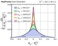
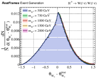
Refer to caption
Refer to caption
Refer to caption
Refer to caption
Figure 12: Distributions of (a) Higgs decay angle, θHsubscript𝜃𝐻\theta_{\mathrm{{\color[rgb]{0.45,0.0,0.09}\definecolor[named]{pgfstrokecolor}{rgb}{0.45,0.0,0.09}\textbf{$H$}}}} and (b) W𝑊W decay angle, θWsubscript𝜃𝑊\theta_{\mathrm{{\color[rgb]{0.45,0.0,0.09}\definecolor[named]{pgfstrokecolor}{rgb}{0.45,0.0,0.09}\textbf{$W$}}}}, estimated using the RJR scheme for simulated H0W+(ν)W(ν)superscript𝐻0superscript𝑊𝜈superscript𝑊𝜈H^{0}\rightarrow W^{+}(\ell\nu)W^{-}(\ell\nu) events and various values for mHsuperscriptsubscript𝑚𝐻absentm_{\footnotesize\mathrm{{\color[rgb]{0.45,0.0,0.09}\definecolor[named]{pgfstrokecolor}{rgb}{0.45,0.0,0.09}\textbf{$H$}}}}^{\footnotesize\leavevmode\nobreak\ }. Figures (c,d) show these estimators as a function of their corresponding mass estimators, MHsuperscriptsubscript𝑀𝐻absentM_{\footnotesize\mathrm{{\color[rgb]{0.45,0.0,0.09}\definecolor[named]{pgfstrokecolor}{rgb}{0.45,0.0,0.09}\textbf{$H$}}}}^{\footnotesize\leavevmode\nobreak\ } and MWsuperscriptsubscript𝑀𝑊absentM_{\footnotesize\mathrm{{\color[rgb]{0.45,0.0,0.09}\definecolor[named]{pgfstrokecolor}{rgb}{0.45,0.0,0.09}\textbf{$W$}}}}^{\footnotesize\leavevmode\nobreak\ }, respectively. Each observable is normalized appropriately by the true value of the quantity it is estimating, with angles in units radian.

The kinematic observables resulting from the RJR approximate reconstruction of these events are also known as super-razor variables, with a thorough discussion of their phenomenology in the corresponding reference Buckley:2013kua .

VI.2 t~t~(tχ10)(tχ10)~𝑡~𝑡𝑡superscriptsubscript𝜒10𝑡superscriptsubscript𝜒10\tilde{t}\tilde{t}\rightarrow(t\chi_{1}^{0})(t\chi_{1}^{0}) at a hadron collider

To further generalize the JR’s for final states with two invisible particles, we consider the example process of stop quark pair production at a hadron collider, with each stop decaying to a top quark and undetected neutralino. We assume that the top quarks decay hadronically, and that each is identified and reconstructed in the detector, with measured four vectors 𝐩talabsuperscriptsubscript𝐩subscript𝑡𝑎lab\mathbf{p}_{\footnotesize\mathrm{{\color[rgb]{0.1,0.1,0.44}\definecolor[named]{pgfstrokecolor}{rgb}{0.1,0.1,0.44}\textbf{$t_{a}$}}}}^{\footnotesize\leavevmode\nobreak\ \mathrm{\textbf{lab}}} and 𝐩tblabsuperscriptsubscript𝐩subscript𝑡𝑏lab\mathbf{p}_{\footnotesize\mathrm{{\color[rgb]{0.1,0.1,0.44}\definecolor[named]{pgfstrokecolor}{rgb}{0.1,0.1,0.44}\textbf{$t_{b}$}}}}^{\footnotesize\leavevmode\nobreak\ \mathrm{\textbf{lab}}}. In a real experiment, there can be significant kinematic dependencies on the efficiency for reconstructing and identifying hadronically decaying top quarks, along with imperfect resolution in estimating the top’s momentum and mass. We neglect these effects in this example, focusing only on shortcomings in event reconstruction due to missing information associated with the escaping neutralinos. Similarly, we assume that the ETmisssuperscriptsubscript𝐸𝑇miss\vec{E}_{T}^{\rm miss}  provides a reliable estimate of the transverse mass of the di-neutralino system, I={χ~a,χ~b}Isubscript~𝜒𝑎subscript~𝜒𝑏\mathrm{{\color[rgb]{0.12,0.3,0.17}\definecolor[named]{pgfstrokecolor}{rgb}{0.12,0.3,0.17}\textbf{I}}}=\{\mathrm{{\color[rgb]{0.12,0.3,0.17}\definecolor[named]{pgfstrokecolor}{rgb}{0.12,0.3,0.17}\textbf{$\tilde{\chi}_{a}$}}},\mathrm{{\color[rgb]{0.12,0.3,0.17}\definecolor[named]{pgfstrokecolor}{rgb}{0.12,0.3,0.17}\textbf{$\tilde{\chi}_{b}$}}}\}, with pI,Tlab=ETmisssuperscriptsubscript𝑝I𝑇labsuperscriptsubscript𝐸𝑇miss\vec{p}_{\footnotesize\mathrm{{\color[rgb]{0.12,0.3,0.17}\definecolor[named]{pgfstrokecolor}{rgb}{0.12,0.3,0.17}\textbf{I}}},T}^{\footnotesize\leavevmode\nobreak\ \mathrm{\textbf{lab}}}=\vec{E}_{T}^{\rm miss}. The decay tree used in analyzing this final state is shown in Fig. 13.
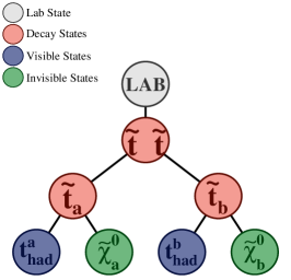
Refer to caption
Figure 13: The decay tree for analyzing t~t~(tχ10)(tχ10)~𝑡~𝑡𝑡superscriptsubscript𝜒10𝑡superscriptsubscript𝜒10\tilde{t}\tilde{t}\rightarrow(t\chi_{1}^{0})(t\chi_{1}^{0}) events. The two sides of the event are labelled “a” and “b”, each including a hadronic top and neutralino from their respective stop decays.

This decay topology is nearly identical to the H0W+(ν)W(ν)superscript𝐻0superscript𝑊𝜈superscript𝑊𝜈H^{0}\rightarrow W^{+}(\ell\nu)W^{-}(\ell\nu) process studied in Section VI.1, with the two intermediate stop quarks playing the role of the W𝑊W bosons. and the di-stop system the neutral Higgs boson. One important difference is that the stop quarks are produced non-resonantly, with mt~t~superscriptsubscript𝑚~𝑡~𝑡absentm_{\footnotesize\mathrm{{\color[rgb]{0.45,0.0,0.09}\definecolor[named]{pgfstrokecolor}{rgb}{0.45,0.0,0.09}\textbf{$\tilde{t}\tilde{t}$}}}}^{\footnotesize\leavevmode\nobreak\ } having a much larger variance than mHsuperscriptsubscript𝑚𝐻absentm_{\footnotesize\mathrm{{\color[rgb]{0.45,0.0,0.09}\definecolor[named]{pgfstrokecolor}{rgb}{0.45,0.0,0.09}\textbf{$H$}}}}^{\footnotesize\leavevmode\nobreak\ }. But this distinction does nothing to prohibit the use of the same event analysis approach described in the previous example. The more pernicious complications follow from the masses of the individual visible tops and neutralinos, which now can have non-negligible values relative to the scale of the process.

These masses have notable implications for the application of a contra-boost invariant JR, like that described in Section VI.1. Taking the same approach, we constrain Mt~a=Mt~bsuperscriptsubscript𝑀subscript~𝑡𝑎absentsuperscriptsubscript𝑀subscript~𝑡𝑏absentM_{\footnotesize\mathrm{{\color[rgb]{0.45,0.0,0.09}\definecolor[named]{pgfstrokecolor}{rgb}{0.45,0.0,0.09}\textbf{$\tilde{t}_{a}$}}}}^{\footnotesize\leavevmode\nobreak\ }=M_{\footnotesize\mathrm{{\color[rgb]{0.45,0.0,0.09}\definecolor[named]{pgfstrokecolor}{rgb}{0.45,0.0,0.09}\textbf{$\tilde{t}_{b}$}}}}^{\footnotesize\leavevmode\nobreak\ }, and use the visible particle four vectors, evaluated in the putative di-stop rest frame, to make guesses for the momentum and energy of the two neutralinos. In the application of the contra-boost invariant JR VI.2 we estimate the velocities relating the di-stop rest frame to the two stop rest frames as

βt~at~t~=βt~bt~t~=ptat~t~ptbt~t~Etat~t~+Etbt~t~.superscriptsubscript𝛽subscript~𝑡𝑎~𝑡~𝑡superscriptsubscript𝛽subscript~𝑡𝑏~𝑡~𝑡superscriptsubscript𝑝subscript𝑡𝑎~𝑡~𝑡superscriptsubscript𝑝subscript𝑡𝑏~𝑡~𝑡superscriptsubscript𝐸subscript𝑡𝑎~𝑡~𝑡superscriptsubscript𝐸subscript𝑡𝑏~𝑡~𝑡\displaystyle\vec{\beta}_{\footnotesize\mathrm{{\color[rgb]{0.45,0.0,0.09}\definecolor[named]{pgfstrokecolor}{rgb}{0.45,0.0,0.09}\textbf{$\tilde{t}_{a}$}}}}^{\footnotesize\leavevmode\nobreak\ \mathrm{{\color[rgb]{0.45,0.0,0.09}\definecolor[named]{pgfstrokecolor}{rgb}{0.45,0.0,0.09}\textbf{$\tilde{t}\tilde{t}$}}}}=-\vec{\beta}_{\footnotesize\mathrm{{\color[rgb]{0.45,0.0,0.09}\definecolor[named]{pgfstrokecolor}{rgb}{0.45,0.0,0.09}\textbf{$\tilde{t}_{b}$}}}}^{\footnotesize\leavevmode\nobreak\ \mathrm{{\color[rgb]{0.45,0.0,0.09}\definecolor[named]{pgfstrokecolor}{rgb}{0.45,0.0,0.09}\textbf{$\tilde{t}\tilde{t}$}}}}=\frac{\vec{p}_{\footnotesize\mathrm{{\color[rgb]{0.1,0.1,0.44}\definecolor[named]{pgfstrokecolor}{rgb}{0.1,0.1,0.44}\textbf{$t_{a}$}}}}^{\footnotesize\leavevmode\nobreak\ \mathrm{{\color[rgb]{0.45,0.0,0.09}\definecolor[named]{pgfstrokecolor}{rgb}{0.45,0.0,0.09}\textbf{$\tilde{t}\tilde{t}$}}}}-\vec{p}_{\footnotesize\mathrm{{\color[rgb]{0.1,0.1,0.44}\definecolor[named]{pgfstrokecolor}{rgb}{0.1,0.1,0.44}\textbf{$t_{b}$}}}}^{\footnotesize\leavevmode\nobreak\ \mathrm{{\color[rgb]{0.45,0.0,0.09}\definecolor[named]{pgfstrokecolor}{rgb}{0.45,0.0,0.09}\textbf{$\tilde{t}\tilde{t}$}}}}}{E_{\footnotesize\mathrm{{\color[rgb]{0.1,0.1,0.44}\definecolor[named]{pgfstrokecolor}{rgb}{0.1,0.1,0.44}\textbf{$t_{a}$}}}}^{\footnotesize\leavevmode\nobreak\ \mathrm{{\color[rgb]{0.45,0.0,0.09}\definecolor[named]{pgfstrokecolor}{rgb}{0.45,0.0,0.09}\textbf{$\tilde{t}\tilde{t}$}}}}+E_{\footnotesize\mathrm{{\color[rgb]{0.1,0.1,0.44}\definecolor[named]{pgfstrokecolor}{rgb}{0.1,0.1,0.44}\textbf{$t_{b}$}}}}^{\footnotesize\leavevmode\nobreak\ \mathrm{{\color[rgb]{0.45,0.0,0.09}\definecolor[named]{pgfstrokecolor}{rgb}{0.45,0.0,0.09}\textbf{$\tilde{t}\tilde{t}$}}}}}\leavevmode\nobreak\ . (16)

This choice constrains the estimators for the neutralino and di-neutralino masses, which can be expressed by an additional free parameter, c𝑐c, in equations analogous to Eq. VI.1:

Mχ~a 2superscriptsubscript𝑀subscript~𝜒𝑎2\displaystyle M_{\footnotesize\mathrm{{\color[rgb]{0.12,0.3,0.17}\definecolor[named]{pgfstrokecolor}{rgb}{0.12,0.3,0.17}\textbf{$\tilde{\chi}_{a}$}}}}^{\footnotesize\leavevmode\nobreak\ 2} =\displaystyle= (c1)2mta 2+c2mtb 2+(c1)cMc2(𝐩tat~t~,𝐩tbt~t~)superscript𝑐12superscriptsubscript𝑚subscript𝑡𝑎2superscript𝑐2superscriptsubscript𝑚subscript𝑡𝑏2𝑐1𝑐superscriptsubscript𝑀𝑐2superscriptsubscript𝐩subscript𝑡𝑎~𝑡~𝑡superscriptsubscript𝐩subscript𝑡𝑏~𝑡~𝑡\displaystyle(c-1)^{2}m_{\footnotesize\mathrm{{\color[rgb]{0.1,0.1,0.44}\definecolor[named]{pgfstrokecolor}{rgb}{0.1,0.1,0.44}\textbf{$t_{a}$}}}}^{\footnotesize\leavevmode\nobreak\ 2}+c^{2}m_{\footnotesize\mathrm{{\color[rgb]{0.1,0.1,0.44}\definecolor[named]{pgfstrokecolor}{rgb}{0.1,0.1,0.44}\textbf{$t_{b}$}}}}^{\footnotesize\leavevmode\nobreak\ 2}+(c-1)cM_{c}^{2}(\mathbf{p}_{\footnotesize\mathrm{{\color[rgb]{0.1,0.1,0.44}\definecolor[named]{pgfstrokecolor}{rgb}{0.1,0.1,0.44}\textbf{$t_{a}$}}}}^{\footnotesize\leavevmode\nobreak\ \mathrm{{\color[rgb]{0.45,0.0,0.09}\definecolor[named]{pgfstrokecolor}{rgb}{0.45,0.0,0.09}\textbf{$\tilde{t}\tilde{t}$}}}},\mathbf{p}_{\footnotesize\mathrm{{\color[rgb]{0.1,0.1,0.44}\definecolor[named]{pgfstrokecolor}{rgb}{0.1,0.1,0.44}\textbf{$t_{b}$}}}}^{\footnotesize\leavevmode\nobreak\ \mathrm{{\color[rgb]{0.45,0.0,0.09}\definecolor[named]{pgfstrokecolor}{rgb}{0.45,0.0,0.09}\textbf{$\tilde{t}\tilde{t}$}}}})
Mχ~b 2superscriptsubscript𝑀subscript~𝜒𝑏2\displaystyle M_{\footnotesize\mathrm{{\color[rgb]{0.12,0.3,0.17}\definecolor[named]{pgfstrokecolor}{rgb}{0.12,0.3,0.17}\textbf{$\tilde{\chi}_{b}$}}}}^{\footnotesize\leavevmode\nobreak\ 2} =\displaystyle= (c1)2mtb 2+c2mta 2+(c1)cMc2(𝐩tat~t~,𝐩tbt~t~)superscript𝑐12superscriptsubscript𝑚subscript𝑡𝑏2superscript𝑐2superscriptsubscript𝑚subscript𝑡𝑎2𝑐1𝑐superscriptsubscript𝑀𝑐2superscriptsubscript𝐩subscript𝑡𝑎~𝑡~𝑡superscriptsubscript𝐩subscript𝑡𝑏~𝑡~𝑡\displaystyle(c-1)^{2}m_{\footnotesize\mathrm{{\color[rgb]{0.1,0.1,0.44}\definecolor[named]{pgfstrokecolor}{rgb}{0.1,0.1,0.44}\textbf{$t_{b}$}}}}^{\footnotesize\leavevmode\nobreak\ 2}+c^{2}m_{\footnotesize\mathrm{{\color[rgb]{0.1,0.1,0.44}\definecolor[named]{pgfstrokecolor}{rgb}{0.1,0.1,0.44}\textbf{$t_{a}$}}}}^{\footnotesize\leavevmode\nobreak\ 2}+(c-1)cM_{c}^{2}(\mathbf{p}_{\footnotesize\mathrm{{\color[rgb]{0.1,0.1,0.44}\definecolor[named]{pgfstrokecolor}{rgb}{0.1,0.1,0.44}\textbf{$t_{a}$}}}}^{\footnotesize\leavevmode\nobreak\ \mathrm{{\color[rgb]{0.45,0.0,0.09}\definecolor[named]{pgfstrokecolor}{rgb}{0.45,0.0,0.09}\textbf{$\tilde{t}\tilde{t}$}}}},\mathbf{p}_{\footnotesize\mathrm{{\color[rgb]{0.1,0.1,0.44}\definecolor[named]{pgfstrokecolor}{rgb}{0.1,0.1,0.44}\textbf{$t_{b}$}}}}^{\footnotesize\leavevmode\nobreak\ \mathrm{{\color[rgb]{0.45,0.0,0.09}\definecolor[named]{pgfstrokecolor}{rgb}{0.45,0.0,0.09}\textbf{$\tilde{t}\tilde{t}$}}}})
MI 2superscriptsubscript𝑀I2\displaystyle M_{\footnotesize\mathrm{{\color[rgb]{0.12,0.3,0.17}\definecolor[named]{pgfstrokecolor}{rgb}{0.12,0.3,0.17}\textbf{I}}}}^{\footnotesize\leavevmode\nobreak\ 2} =\displaystyle= (2c1)2(EVt~t~)2|pVt~t~|2,superscript2𝑐12superscriptsuperscriptsubscript𝐸V~𝑡~𝑡2superscriptsuperscriptsubscript𝑝V~𝑡~𝑡2\displaystyle(2c-1)^{2}(E_{\footnotesize\mathrm{{\color[rgb]{0.1,0.1,0.44}\definecolor[named]{pgfstrokecolor}{rgb}{0.1,0.1,0.44}\textbf{V}}}}^{\footnotesize\leavevmode\nobreak\ \mathrm{{\color[rgb]{0.45,0.0,0.09}\definecolor[named]{pgfstrokecolor}{rgb}{0.45,0.0,0.09}\textbf{$\tilde{t}\tilde{t}$}}}})^{2}-|\vec{p}_{\footnotesize\mathrm{{\color[rgb]{0.1,0.1,0.44}\definecolor[named]{pgfstrokecolor}{rgb}{0.1,0.1,0.44}\textbf{V}}}}^{\footnotesize\leavevmode\nobreak\ \mathrm{{\color[rgb]{0.45,0.0,0.09}\definecolor[named]{pgfstrokecolor}{rgb}{0.45,0.0,0.09}\textbf{$\tilde{t}\tilde{t}$}}}}|^{2}\leavevmode\nobreak\ , (17)

where V={ta,tb}Vsubscript𝑡𝑎subscript𝑡𝑏\mathrm{{\color[rgb]{0.1,0.1,0.44}\definecolor[named]{pgfstrokecolor}{rgb}{0.1,0.1,0.44}\textbf{V}}}=\{\mathrm{{\color[rgb]{0.1,0.1,0.44}\definecolor[named]{pgfstrokecolor}{rgb}{0.1,0.1,0.44}\textbf{$t_{a}$}}},\mathrm{{\color[rgb]{0.1,0.1,0.44}\definecolor[named]{pgfstrokecolor}{rgb}{0.1,0.1,0.44}\textbf{$t_{b}$}}}\} is the collection of all visible particles resulting from the interaction of interest. While appropriate in the previous example, the simple choice MI=mVsuperscriptsubscript𝑀Iabsentsuperscriptsubscript𝑚VabsentM_{\footnotesize\mathrm{{\color[rgb]{0.12,0.3,0.17}\definecolor[named]{pgfstrokecolor}{rgb}{0.12,0.3,0.17}\textbf{I}}}}^{\footnotesize\leavevmode\nobreak\ }=m_{\footnotesize\mathrm{{\color[rgb]{0.1,0.1,0.44}\definecolor[named]{pgfstrokecolor}{rgb}{0.1,0.1,0.44}\textbf{V}}}}^{\footnotesize\leavevmode\nobreak\ } would result in each of the neutralinos taking nonzero masses, with Mχ~a/b=mtb/asuperscriptsubscript𝑀subscript~𝜒𝑎𝑏absentsuperscriptsubscript𝑚subscript𝑡𝑏𝑎absentM_{\footnotesize\mathrm{{\color[rgb]{0.12,0.3,0.17}\definecolor[named]{pgfstrokecolor}{rgb}{0.12,0.3,0.17}\textbf{$\tilde{\chi}_{a/b}$}}}}^{\footnotesize\leavevmode\nobreak\ }=m_{\footnotesize\mathrm{{\color[rgb]{0.1,0.1,0.44}\definecolor[named]{pgfstrokecolor}{rgb}{0.1,0.1,0.44}\textbf{$t_{b/a}$}}}}^{\footnotesize\leavevmode\nobreak\ }. For the moment, we assume that mta=mtb=mtsuperscriptsubscript𝑚subscript𝑡𝑎absentsuperscriptsubscript𝑚subscript𝑡𝑏absentsuperscriptsubscript𝑚𝑡absentm_{\footnotesize\mathrm{{\color[rgb]{0.1,0.1,0.44}\definecolor[named]{pgfstrokecolor}{rgb}{0.1,0.1,0.44}\textbf{$t_{a}$}}}}^{\footnotesize\leavevmode\nobreak\ }=m_{\footnotesize\mathrm{{\color[rgb]{0.1,0.1,0.44}\definecolor[named]{pgfstrokecolor}{rgb}{0.1,0.1,0.44}\textbf{$t_{b}$}}}}^{\footnotesize\leavevmode\nobreak\ }=m_{\footnotesize\mathrm{{\color[rgb]{0.1,0.1,0.44}\definecolor[named]{pgfstrokecolor}{rgb}{0.1,0.1,0.44}\textbf{$t$}}}}^{\footnotesize\leavevmode\nobreak\ } to simplify the discussion, generalizing later. If we instead attempt to constrain this final degree of freedom by requiring Mχ~a=Mχ~b=0superscriptsubscript𝑀subscript~𝜒𝑎absentsuperscriptsubscript𝑀subscript~𝜒𝑏absent0M_{\footnotesize\mathrm{{\color[rgb]{0.12,0.3,0.17}\definecolor[named]{pgfstrokecolor}{rgb}{0.12,0.3,0.17}\textbf{$\tilde{\chi}_{a}$}}}}^{\footnotesize\leavevmode\nobreak\ }=M_{\footnotesize\mathrm{{\color[rgb]{0.12,0.3,0.17}\definecolor[named]{pgfstrokecolor}{rgb}{0.12,0.3,0.17}\textbf{$\tilde{\chi}_{b}$}}}}^{\footnotesize\leavevmode\nobreak\ }=0, for lack of a better choice, this implies an expression for MIsuperscriptsubscript𝑀IabsentM_{\footnotesize\mathrm{{\color[rgb]{0.12,0.3,0.17}\definecolor[named]{pgfstrokecolor}{rgb}{0.12,0.3,0.17}\textbf{I}}}}^{\footnotesize\leavevmode\nobreak\ } of

MI 2|Mχ~=0=4(|ptat~t~|2|ptbt~t~|2(ptat~t~ptbt~t~)2)2mt 2+Mc2(𝐩tat~t~,𝐩tbt~t~).evaluated-atsuperscriptsubscript𝑀I2superscriptsubscript𝑀~𝜒absent04superscriptsuperscriptsubscript𝑝subscript𝑡𝑎~𝑡~𝑡2superscriptsuperscriptsubscript𝑝subscript𝑡𝑏~𝑡~𝑡2superscriptsuperscriptsubscript𝑝subscript𝑡𝑎~𝑡~𝑡superscriptsubscript𝑝subscript𝑡𝑏~𝑡~𝑡22superscriptsubscript𝑚𝑡2superscriptsubscript𝑀𝑐2superscriptsubscript𝐩subscript𝑡𝑎~𝑡~𝑡superscriptsubscript𝐩subscript𝑡𝑏~𝑡~𝑡\displaystyle M_{\footnotesize\mathrm{{\color[rgb]{0.12,0.3,0.17}\definecolor[named]{pgfstrokecolor}{rgb}{0.12,0.3,0.17}\textbf{I}}}}^{\footnotesize\leavevmode\nobreak\ 2}|_{M_{\footnotesize\mathrm{{\color[rgb]{0.12,0.3,0.17}\definecolor[named]{pgfstrokecolor}{rgb}{0.12,0.3,0.17}\textbf{$\tilde{\chi}$}}}}^{\footnotesize\leavevmode\nobreak\ }=0}=\frac{4\left(|\vec{p}_{\footnotesize\mathrm{{\color[rgb]{0.1,0.1,0.44}\definecolor[named]{pgfstrokecolor}{rgb}{0.1,0.1,0.44}\textbf{$t_{a}$}}}}^{\footnotesize\leavevmode\nobreak\ \mathrm{{\color[rgb]{0.45,0.0,0.09}\definecolor[named]{pgfstrokecolor}{rgb}{0.45,0.0,0.09}\textbf{$\tilde{t}\tilde{t}$}}}}|^{2}|\vec{p}_{\footnotesize\mathrm{{\color[rgb]{0.1,0.1,0.44}\definecolor[named]{pgfstrokecolor}{rgb}{0.1,0.1,0.44}\textbf{$t_{b}$}}}}^{\footnotesize\leavevmode\nobreak\ \mathrm{{\color[rgb]{0.45,0.0,0.09}\definecolor[named]{pgfstrokecolor}{rgb}{0.45,0.0,0.09}\textbf{$\tilde{t}\tilde{t}$}}}}|^{2}-(\vec{p}_{\footnotesize\mathrm{{\color[rgb]{0.1,0.1,0.44}\definecolor[named]{pgfstrokecolor}{rgb}{0.1,0.1,0.44}\textbf{$t_{a}$}}}}^{\footnotesize\leavevmode\nobreak\ \mathrm{{\color[rgb]{0.45,0.0,0.09}\definecolor[named]{pgfstrokecolor}{rgb}{0.45,0.0,0.09}\textbf{$\tilde{t}\tilde{t}$}}}}\cdot\vec{p}_{\footnotesize\mathrm{{\color[rgb]{0.1,0.1,0.44}\definecolor[named]{pgfstrokecolor}{rgb}{0.1,0.1,0.44}\textbf{$t_{b}$}}}}^{\footnotesize\leavevmode\nobreak\ \mathrm{{\color[rgb]{0.45,0.0,0.09}\definecolor[named]{pgfstrokecolor}{rgb}{0.45,0.0,0.09}\textbf{$\tilde{t}\tilde{t}$}}}})^{2}\right)}{2m_{\footnotesize\mathrm{{\color[rgb]{0.1,0.1,0.44}\definecolor[named]{pgfstrokecolor}{rgb}{0.1,0.1,0.44}\textbf{$t$}}}}^{\footnotesize\leavevmode\nobreak\ 2}+M_{c}^{2}(\mathbf{p}_{\footnotesize\mathrm{{\color[rgb]{0.1,0.1,0.44}\definecolor[named]{pgfstrokecolor}{rgb}{0.1,0.1,0.44}\textbf{$t_{a}$}}}}^{\footnotesize\leavevmode\nobreak\ \mathrm{{\color[rgb]{0.45,0.0,0.09}\definecolor[named]{pgfstrokecolor}{rgb}{0.45,0.0,0.09}\textbf{$\tilde{t}\tilde{t}$}}}},\mathbf{p}_{\footnotesize\mathrm{{\color[rgb]{0.1,0.1,0.44}\definecolor[named]{pgfstrokecolor}{rgb}{0.1,0.1,0.44}\textbf{$t_{b}$}}}}^{\footnotesize\leavevmode\nobreak\ \mathrm{{\color[rgb]{0.45,0.0,0.09}\definecolor[named]{pgfstrokecolor}{rgb}{0.45,0.0,0.09}\textbf{$\tilde{t}\tilde{t}$}}}})}\leavevmode\nobreak\ . (18)

Unfortunately, this is not a viable choice for MIsuperscriptsubscript𝑀IabsentM_{\footnotesize\mathrm{{\color[rgb]{0.12,0.3,0.17}\definecolor[named]{pgfstrokecolor}{rgb}{0.12,0.3,0.17}\textbf{I}}}}^{\footnotesize\leavevmode\nobreak\ }, as its expression in Eq. 18 is not a Lorentz invariant function of the visible four vectors, which violates one of the requirements of the invisible mass JR VI.1 we must apply in order to calculate the velocity relating the lab frame to the di-stop rest frame, βt~t~labsuperscriptsubscript𝛽~𝑡~𝑡lab\vec{\beta}_{\footnotesize\mathrm{{\color[rgb]{0.45,0.0,0.09}\definecolor[named]{pgfstrokecolor}{rgb}{0.45,0.0,0.09}\textbf{$\tilde{t}\tilde{t}$}}}}^{\footnotesize\leavevmode\nobreak\ \mathrm{\textbf{lab}}}. One could imagine trying to remedy this situation through a brute-force approach, writing Eq. 18 as a function of this unknown velocity by boosting the top four vectors from the lab frame to the di-stop rest frame, and further constraining MIsuperscriptsubscript𝑀IabsentM_{\footnotesize\mathrm{{\color[rgb]{0.12,0.3,0.17}\definecolor[named]{pgfstrokecolor}{rgb}{0.12,0.3,0.17}\textbf{I}}}}^{\footnotesize\leavevmode\nobreak\ } and βt~t~labsuperscriptsubscript𝛽~𝑡~𝑡lab\vec{\beta}_{\footnotesize\mathrm{{\color[rgb]{0.45,0.0,0.09}\definecolor[named]{pgfstrokecolor}{rgb}{0.45,0.0,0.09}\textbf{$\tilde{t}\tilde{t}$}}}}^{\footnotesize\leavevmode\nobreak\ \mathrm{\textbf{lab}}} through the relation

βt~t~lab=pt~t~labEVlab+|pIlab|2+MI 2(βt~t~lab).superscriptsubscript𝛽~𝑡~𝑡labsuperscriptsubscript𝑝~𝑡~𝑡labsuperscriptsubscript𝐸Vlabsuperscriptsuperscriptsubscript𝑝Ilab2superscriptsubscript𝑀I2superscriptsubscript𝛽~𝑡~𝑡lab\displaystyle\vec{\beta}_{\footnotesize\mathrm{{\color[rgb]{0.45,0.0,0.09}\definecolor[named]{pgfstrokecolor}{rgb}{0.45,0.0,0.09}\textbf{$\tilde{t}\tilde{t}$}}}}^{\footnotesize\leavevmode\nobreak\ \mathrm{\textbf{lab}}}=\frac{\vec{p}_{\footnotesize\mathrm{{\color[rgb]{0.45,0.0,0.09}\definecolor[named]{pgfstrokecolor}{rgb}{0.45,0.0,0.09}\textbf{$\tilde{t}\tilde{t}$}}}}^{\footnotesize\leavevmode\nobreak\ \mathrm{\textbf{lab}}}}{E_{\footnotesize\mathrm{{\color[rgb]{0.1,0.1,0.44}\definecolor[named]{pgfstrokecolor}{rgb}{0.1,0.1,0.44}\textbf{V}}}}^{\footnotesize\leavevmode\nobreak\ \mathrm{\textbf{lab}}}+\sqrt{|\vec{p}_{\footnotesize\mathrm{{\color[rgb]{0.12,0.3,0.17}\definecolor[named]{pgfstrokecolor}{rgb}{0.12,0.3,0.17}\textbf{I}}}}^{\footnotesize\leavevmode\nobreak\ \mathrm{\textbf{lab}}}|^{2}+M_{\footnotesize\mathrm{{\color[rgb]{0.12,0.3,0.17}\definecolor[named]{pgfstrokecolor}{rgb}{0.12,0.3,0.17}\textbf{I}}}}^{\footnotesize\leavevmode\nobreak\ 2}(\vec{\beta}_{\footnotesize\mathrm{{\color[rgb]{0.45,0.0,0.09}\definecolor[named]{pgfstrokecolor}{rgb}{0.45,0.0,0.09}\textbf{$\tilde{t}\tilde{t}$}}}}^{\footnotesize\leavevmode\nobreak\ \mathrm{\textbf{lab}}})}}\leavevmode\nobreak\ . (19)

Although numerically viable, solving Eq. 19 for βt~t~labsuperscriptsubscript𝛽~𝑡~𝑡lab\vec{\beta}_{\footnotesize\mathrm{{\color[rgb]{0.45,0.0,0.09}\definecolor[named]{pgfstrokecolor}{rgb}{0.45,0.0,0.09}\textbf{$\tilde{t}\tilde{t}$}}}}^{\footnotesize\leavevmode\nobreak\ \mathrm{\textbf{lab}}}, a high order polynomial equation, will lead to multiple solutions, none of which are guaranteed to be real.

We choose to take a different approach, effectively factorizing the JR’s applied at different stages in the decay tree by choosing MIsuperscriptsubscript𝑀IabsentM_{\footnotesize\mathrm{{\color[rgb]{0.12,0.3,0.17}\definecolor[named]{pgfstrokecolor}{rgb}{0.12,0.3,0.17}\textbf{I}}}}^{\footnotesize\leavevmode\nobreak\ } as the smallest Lorentz invariant expression that is strictly greater or equal to that in Eq. 18:

MI 2=mV 24mt 2MI 2|Mχ~=0.superscriptsubscript𝑀I2superscriptsubscript𝑚V24superscriptsubscript𝑚𝑡2evaluated-atsuperscriptsubscript𝑀I2superscriptsubscript𝑀~𝜒absent0\displaystyle M_{\footnotesize\mathrm{{\color[rgb]{0.12,0.3,0.17}\definecolor[named]{pgfstrokecolor}{rgb}{0.12,0.3,0.17}\textbf{I}}}}^{\footnotesize\leavevmode\nobreak\ 2}=m_{\footnotesize\mathrm{{\color[rgb]{0.1,0.1,0.44}\definecolor[named]{pgfstrokecolor}{rgb}{0.1,0.1,0.44}\textbf{V}}}}^{\footnotesize\leavevmode\nobreak\ 2}-4m_{\footnotesize\mathrm{{\color[rgb]{0.1,0.1,0.44}\definecolor[named]{pgfstrokecolor}{rgb}{0.1,0.1,0.44}\textbf{$t$}}}}^{\footnotesize\leavevmode\nobreak\ 2}\geq M_{\footnotesize\mathrm{{\color[rgb]{0.12,0.3,0.17}\definecolor[named]{pgfstrokecolor}{rgb}{0.12,0.3,0.17}\textbf{I}}}}^{\footnotesize\leavevmode\nobreak\ 2}|_{M_{\footnotesize\mathrm{{\color[rgb]{0.12,0.3,0.17}\definecolor[named]{pgfstrokecolor}{rgb}{0.12,0.3,0.17}\textbf{$\tilde{\chi}$}}}}^{\footnotesize\leavevmode\nobreak\ }=0}\leavevmode\nobreak\ . (20)

That this expression is Lorentz invariant means it can be evaluated using only the four vectors of visible particles measured in the lab frame, and doesn’t require knowledge of any approximate reference frames in the event. But this choice also requires a concession, in that our estimators for the neutrinalino masses, Mχ~asuperscriptsubscript𝑀subscript~𝜒𝑎absentM_{\footnotesize\mathrm{{\color[rgb]{0.12,0.3,0.17}\definecolor[named]{pgfstrokecolor}{rgb}{0.12,0.3,0.17}\textbf{$\tilde{\chi}_{a}$}}}}^{\footnotesize\leavevmode\nobreak\ } and Mχ~bsuperscriptsubscript𝑀subscript~𝜒𝑏absentM_{\footnotesize\mathrm{{\color[rgb]{0.12,0.3,0.17}\definecolor[named]{pgfstrokecolor}{rgb}{0.12,0.3,0.17}\textbf{$\tilde{\chi}_{b}$}}}}^{\footnotesize\leavevmode\nobreak\ }, which we previously tried to constrain to zero, will now take non-zero values, with

Mχ~a/b=mt|ptat~t~ptbt~t~|Etat~t~+Etbt~t~.superscriptsubscript𝑀subscript~𝜒𝑎𝑏absentsuperscriptsubscript𝑚𝑡absentsuperscriptsubscript𝑝subscript𝑡𝑎~𝑡~𝑡superscriptsubscript𝑝subscript𝑡𝑏~𝑡~𝑡superscriptsubscript𝐸subscript𝑡𝑎~𝑡~𝑡superscriptsubscript𝐸subscript𝑡𝑏~𝑡~𝑡\displaystyle M_{\footnotesize\mathrm{{\color[rgb]{0.12,0.3,0.17}\definecolor[named]{pgfstrokecolor}{rgb}{0.12,0.3,0.17}\textbf{$\tilde{\chi}_{a/b}$}}}}^{\footnotesize\leavevmode\nobreak\ }=m_{\footnotesize\mathrm{{\color[rgb]{0.1,0.1,0.44}\definecolor[named]{pgfstrokecolor}{rgb}{0.1,0.1,0.44}\textbf{$t$}}}}^{\footnotesize\leavevmode\nobreak\ }\frac{|\vec{p}_{\footnotesize\mathrm{{\color[rgb]{0.1,0.1,0.44}\definecolor[named]{pgfstrokecolor}{rgb}{0.1,0.1,0.44}\textbf{$t_{a}$}}}}^{\footnotesize\leavevmode\nobreak\ \mathrm{{\color[rgb]{0.45,0.0,0.09}\definecolor[named]{pgfstrokecolor}{rgb}{0.45,0.0,0.09}\textbf{$\tilde{t}\tilde{t}$}}}}-\vec{p}_{\footnotesize\mathrm{{\color[rgb]{0.1,0.1,0.44}\definecolor[named]{pgfstrokecolor}{rgb}{0.1,0.1,0.44}\textbf{$t_{b}$}}}}^{\footnotesize\leavevmode\nobreak\ \mathrm{{\color[rgb]{0.45,0.0,0.09}\definecolor[named]{pgfstrokecolor}{rgb}{0.45,0.0,0.09}\textbf{$\tilde{t}\tilde{t}$}}}}|}{E_{\footnotesize\mathrm{{\color[rgb]{0.1,0.1,0.44}\definecolor[named]{pgfstrokecolor}{rgb}{0.1,0.1,0.44}\textbf{$t_{a}$}}}}^{\footnotesize\leavevmode\nobreak\ \mathrm{{\color[rgb]{0.45,0.0,0.09}\definecolor[named]{pgfstrokecolor}{rgb}{0.45,0.0,0.09}\textbf{$\tilde{t}\tilde{t}$}}}}+E_{\footnotesize\mathrm{{\color[rgb]{0.1,0.1,0.44}\definecolor[named]{pgfstrokecolor}{rgb}{0.1,0.1,0.44}\textbf{$t_{b}$}}}}^{\footnotesize\leavevmode\nobreak\ \mathrm{{\color[rgb]{0.45,0.0,0.09}\definecolor[named]{pgfstrokecolor}{rgb}{0.45,0.0,0.09}\textbf{$\tilde{t}\tilde{t}$}}}}}\leavevmode\nobreak\ . (21)

A portion of the “extra” mass we assigned to MIsuperscriptsubscript𝑀IabsentM_{\footnotesize\mathrm{{\color[rgb]{0.12,0.3,0.17}\definecolor[named]{pgfstrokecolor}{rgb}{0.12,0.3,0.17}\textbf{I}}}}^{\footnotesize\leavevmode\nobreak\ } in Eq. 20 in order to make it Lorentz invariant has been absorbed by Mχ~a/bsuperscriptsubscript𝑀subscript~𝜒𝑎𝑏absentM_{\footnotesize\mathrm{{\color[rgb]{0.12,0.3,0.17}\definecolor[named]{pgfstrokecolor}{rgb}{0.12,0.3,0.17}\textbf{$\tilde{\chi}_{a/b}$}}}}^{\footnotesize\leavevmode\nobreak\ }. The expression does not contain new information, in the sense that it is a combination of mtsuperscriptsubscript𝑚𝑡absentm_{\footnotesize\mathrm{{\color[rgb]{0.1,0.1,0.44}\definecolor[named]{pgfstrokecolor}{rgb}{0.1,0.1,0.44}\textbf{$t$}}}}^{\footnotesize\leavevmode\nobreak\ } and the estimator for βt~a/bt~t~superscriptsubscript𝛽subscript~𝑡𝑎𝑏~𝑡~𝑡\vec{\beta}_{\footnotesize\mathrm{{\color[rgb]{0.45,0.0,0.09}\definecolor[named]{pgfstrokecolor}{rgb}{0.45,0.0,0.09}\textbf{$\tilde{t}_{a/b}$}}}}^{\footnotesize\leavevmode\nobreak\ \mathrm{{\color[rgb]{0.45,0.0,0.09}\definecolor[named]{pgfstrokecolor}{rgb}{0.45,0.0,0.09}\textbf{$\tilde{t}\tilde{t}$}}}} from Eq. 16, and is not sensitive to the true values mχ~a/bsuperscriptsubscript𝑚subscript~𝜒𝑎𝑏absentm_{\footnotesize\mathrm{{\color[rgb]{0.12,0.3,0.17}\definecolor[named]{pgfstrokecolor}{rgb}{0.12,0.3,0.17}\textbf{$\tilde{\chi}_{a/b}$}}}}^{\footnotesize\leavevmode\nobreak\ }. We also note that our estimators for the top energies in their respective production frames, Etat~asuperscriptsubscript𝐸subscript𝑡𝑎subscript~𝑡𝑎E_{\footnotesize\mathrm{{\color[rgb]{0.1,0.1,0.44}\definecolor[named]{pgfstrokecolor}{rgb}{0.1,0.1,0.44}\textbf{$t_{a}$}}}}^{\footnotesize\leavevmode\nobreak\ \mathrm{{\color[rgb]{0.45,0.0,0.09}\definecolor[named]{pgfstrokecolor}{rgb}{0.45,0.0,0.09}\textbf{$\tilde{t}_{a}$}}}} and Etbt~bsuperscriptsubscript𝐸subscript𝑡𝑏subscript~𝑡𝑏E_{\footnotesize\mathrm{{\color[rgb]{0.1,0.1,0.44}\definecolor[named]{pgfstrokecolor}{rgb}{0.1,0.1,0.44}\textbf{$t_{b}$}}}}^{\footnotesize\leavevmode\nobreak\ \mathrm{{\color[rgb]{0.45,0.0,0.09}\definecolor[named]{pgfstrokecolor}{rgb}{0.45,0.0,0.09}\textbf{$\tilde{t}_{b}$}}}}, do not depend on this choice of MIsuperscriptsubscript𝑀IabsentM_{\footnotesize\mathrm{{\color[rgb]{0.12,0.3,0.17}\definecolor[named]{pgfstrokecolor}{rgb}{0.12,0.3,0.17}\textbf{I}}}}^{\footnotesize\leavevmode\nobreak\ }, with

Eta/bt~a/b=2mt 2+Mc2(𝐩tat~t~,𝐩tbt~t~)2.superscriptsubscript𝐸subscript𝑡𝑎𝑏subscript~𝑡𝑎𝑏2superscriptsubscript𝑚𝑡2superscriptsubscript𝑀𝑐2superscriptsubscript𝐩subscript𝑡𝑎~𝑡~𝑡superscriptsubscript𝐩subscript𝑡𝑏~𝑡~𝑡2\displaystyle E_{\footnotesize\mathrm{{\color[rgb]{0.1,0.1,0.44}\definecolor[named]{pgfstrokecolor}{rgb}{0.1,0.1,0.44}\textbf{$t_{a/b}$}}}}^{\footnotesize\leavevmode\nobreak\ \mathrm{{\color[rgb]{0.45,0.0,0.09}\definecolor[named]{pgfstrokecolor}{rgb}{0.45,0.0,0.09}\textbf{$\tilde{t}_{a/b}$}}}}=\frac{\sqrt{2m_{\footnotesize\mathrm{{\color[rgb]{0.1,0.1,0.44}\definecolor[named]{pgfstrokecolor}{rgb}{0.1,0.1,0.44}\textbf{$t$}}}}^{\footnotesize\leavevmode\nobreak\ 2}+M_{c}^{2}(\mathbf{p}_{\footnotesize\mathrm{{\color[rgb]{0.1,0.1,0.44}\definecolor[named]{pgfstrokecolor}{rgb}{0.1,0.1,0.44}\textbf{$t_{a}$}}}}^{\footnotesize\leavevmode\nobreak\ \mathrm{{\color[rgb]{0.45,0.0,0.09}\definecolor[named]{pgfstrokecolor}{rgb}{0.45,0.0,0.09}\textbf{$\tilde{t}\tilde{t}$}}}},\mathbf{p}_{\footnotesize\mathrm{{\color[rgb]{0.1,0.1,0.44}\definecolor[named]{pgfstrokecolor}{rgb}{0.1,0.1,0.44}\textbf{$t_{b}$}}}}^{\footnotesize\leavevmode\nobreak\ \mathrm{{\color[rgb]{0.45,0.0,0.09}\definecolor[named]{pgfstrokecolor}{rgb}{0.45,0.0,0.09}\textbf{$\tilde{t}\tilde{t}$}}}})}}{2}\leavevmode\nobreak\ . (22)

Recalling that Eta/bt~a/b=(mt~a/b 2mχ~a/b 2+mta/b 2)/2mt~a/bsuperscriptsubscript𝐸subscript𝑡𝑎𝑏subscript~𝑡𝑎𝑏superscriptsubscript𝑚subscript~𝑡𝑎𝑏2superscriptsubscript𝑚subscript~𝜒𝑎𝑏2superscriptsubscript𝑚subscript𝑡𝑎𝑏22superscriptsubscript𝑚subscript~𝑡𝑎𝑏absentE_{\footnotesize\mathrm{{\color[rgb]{0.1,0.1,0.44}\definecolor[named]{pgfstrokecolor}{rgb}{0.1,0.1,0.44}\textbf{$t_{a/b}$}}}}^{\footnotesize\leavevmode\nobreak\ \mathrm{{\color[rgb]{0.45,0.0,0.09}\definecolor[named]{pgfstrokecolor}{rgb}{0.45,0.0,0.09}\textbf{$\tilde{t}_{a/b}$}}}}=(m_{\footnotesize\mathrm{{\color[rgb]{0.45,0.0,0.09}\definecolor[named]{pgfstrokecolor}{rgb}{0.45,0.0,0.09}\textbf{$\tilde{t}_{a/b}$}}}}^{\footnotesize\leavevmode\nobreak\ 2}-m_{\footnotesize\mathrm{{\color[rgb]{0.12,0.3,0.17}\definecolor[named]{pgfstrokecolor}{rgb}{0.12,0.3,0.17}\textbf{$\tilde{\chi}_{a/b}$}}}}^{\footnotesize\leavevmode\nobreak\ 2}+m_{\footnotesize\mathrm{{\color[rgb]{0.1,0.1,0.44}\definecolor[named]{pgfstrokecolor}{rgb}{0.1,0.1,0.44}\textbf{$t_{a/b}$}}}}^{\footnotesize\leavevmode\nobreak\ 2})/2m_{\footnotesize\mathrm{{\color[rgb]{0.45,0.0,0.09}\definecolor[named]{pgfstrokecolor}{rgb}{0.45,0.0,0.09}\textbf{$\tilde{t}_{a/b}$}}}}^{\footnotesize\leavevmode\nobreak\ }, we are reminded that we are only sensitive to the mass difference between stops and neutralinos in these events, and our estimator of this quantity, Eta/bt~a/bsuperscriptsubscript𝐸subscript𝑡𝑎𝑏subscript~𝑡𝑎𝑏E_{\footnotesize\mathrm{{\color[rgb]{0.1,0.1,0.44}\definecolor[named]{pgfstrokecolor}{rgb}{0.1,0.1,0.44}\textbf{$t_{a/b}$}}}}^{\footnotesize\leavevmode\nobreak\ \mathrm{{\color[rgb]{0.45,0.0,0.09}\definecolor[named]{pgfstrokecolor}{rgb}{0.45,0.0,0.09}\textbf{$\tilde{t}_{a/b}$}}}}, can be extracted with contra-boost invariance independent of our choices for the individual neutralino masses. In practice, allowing our estimators Mχ~a/bsuperscriptsubscript𝑀subscript~𝜒𝑎𝑏absentM_{\footnotesize\mathrm{{\color[rgb]{0.12,0.3,0.17}\definecolor[named]{pgfstrokecolor}{rgb}{0.12,0.3,0.17}\textbf{$\tilde{\chi}_{a/b}$}}}}^{\footnotesize\leavevmode\nobreak\ } to acquire mass in our approximate view of each event is a book-keeping device to account for the lack of commutation between the boosts (βt~t~labsuperscriptsubscript𝛽~𝑡~𝑡lab\vec{\beta}_{\footnotesize\mathrm{{\color[rgb]{0.45,0.0,0.09}\definecolor[named]{pgfstrokecolor}{rgb}{0.45,0.0,0.09}\textbf{$\tilde{t}\tilde{t}$}}}}^{\footnotesize\leavevmode\nobreak\ \mathrm{\textbf{lab}}}) and contra-boosts (βt~a/bt~t~superscriptsubscript𝛽subscript~𝑡𝑎𝑏~𝑡~𝑡\vec{\beta}_{\footnotesize\mathrm{{\color[rgb]{0.45,0.0,0.09}\definecolor[named]{pgfstrokecolor}{rgb}{0.45,0.0,0.09}\textbf{$\tilde{t}_{a/b}$}}}}^{\footnotesize\leavevmode\nobreak\ \mathrm{{\color[rgb]{0.45,0.0,0.09}\definecolor[named]{pgfstrokecolor}{rgb}{0.45,0.0,0.09}\textbf{$\tilde{t}\tilde{t}$}}}}) which describe the visible tops’ path from their production frames to the lab frame. While providing no information about the true mass values of the invisible particles, this approach minimizes the effect this lack of knowledge has on our ability to extract other information from the event, like the mass splittings of sparticles. It also allows for the JR’s applied in analyzing the event to be factorized and, as we will see in later examples, inter-changed, further decoupling the observables measured in each approximate reference frame.

In service of this last consideration, we imagine a case where one may want to ensure that the estimators Mχ~a/bsuperscriptsubscript𝑀subscript~𝜒𝑎𝑏absentM_{\footnotesize\mathrm{{\color[rgb]{0.12,0.3,0.17}\definecolor[named]{pgfstrokecolor}{rgb}{0.12,0.3,0.17}\textbf{$\tilde{\chi}_{a/b}$}}}}^{\footnotesize\leavevmode\nobreak\ }, and the corresponding quantities in our reconstructed view of each event, are greater than or equal to some non-trivial value, with Mχ~a/bμsuperscriptsubscript𝑀subscript~𝜒𝑎𝑏absent𝜇M_{\footnotesize\mathrm{{\color[rgb]{0.12,0.3,0.17}\definecolor[named]{pgfstrokecolor}{rgb}{0.12,0.3,0.17}\textbf{$\tilde{\chi}_{a/b}$}}}}^{\footnotesize\leavevmode\nobreak\ }\geq\mu. This need may occur if there is prior knowledge, outside of quantities measured in the event, about these masses, or if one wants to examine the dependence of observables in different test masses Mminsubscript𝑀minM_{\rm min}. Allowing for a minimum mass also permits this contra-boost invariant JR to accommodate future invisible JR’s appearing later in the decay tree, where χ~asubscript~𝜒𝑎\tilde{\chi}_{a} and χ~bsubscript~𝜒𝑏\tilde{\chi}_{b} may be sub-divided into more invisible particles.

Returning to Eq. VI.2, requiring Mχ~a/b=μsuperscriptsubscript𝑀subscript~𝜒𝑎𝑏absent𝜇M_{\footnotesize\mathrm{{\color[rgb]{0.12,0.3,0.17}\definecolor[named]{pgfstrokecolor}{rgb}{0.12,0.3,0.17}\textbf{$\tilde{\chi}_{a/b}$}}}}^{\footnotesize\leavevmode\nobreak\ }=\mu implies that MIsuperscriptsubscript𝑀IabsentM_{\footnotesize\mathrm{{\color[rgb]{0.12,0.3,0.17}\definecolor[named]{pgfstrokecolor}{rgb}{0.12,0.3,0.17}\textbf{I}}}}^{\footnotesize\leavevmode\nobreak\ } can be expressed as

MI 2|Mχ~=μevaluated-atsuperscriptsubscript𝑀I2superscriptsubscript𝑀~𝜒absent𝜇\displaystyle M_{\footnotesize\mathrm{{\color[rgb]{0.12,0.3,0.17}\definecolor[named]{pgfstrokecolor}{rgb}{0.12,0.3,0.17}\textbf{I}}}}^{\footnotesize\leavevmode\nobreak\ 2}|_{M_{\footnotesize\mathrm{{\color[rgb]{0.12,0.3,0.17}\definecolor[named]{pgfstrokecolor}{rgb}{0.12,0.3,0.17}\textbf{$\tilde{\chi}$}}}}^{\footnotesize\leavevmode\nobreak\ }=\mu} =\displaystyle=
mV 2superscriptsubscript𝑚V2\displaystyle m_{\footnotesize\mathrm{{\color[rgb]{0.1,0.1,0.44}\definecolor[named]{pgfstrokecolor}{rgb}{0.1,0.1,0.44}\textbf{V}}}}^{\footnotesize\leavevmode\nobreak\ 2} +\displaystyle+ 4(μ2mt 2)2mt 2+Mc2(𝐩tat~t~,𝐩tbt~t~)(EVt~t~)2.4superscript𝜇2superscriptsubscript𝑚𝑡22superscriptsubscript𝑚𝑡2superscriptsubscript𝑀𝑐2superscriptsubscript𝐩subscript𝑡𝑎~𝑡~𝑡superscriptsubscript𝐩subscript𝑡𝑏~𝑡~𝑡superscriptsuperscriptsubscript𝐸V~𝑡~𝑡2\displaystyle\frac{4(\mu^{2}-m_{\footnotesize\mathrm{{\color[rgb]{0.1,0.1,0.44}\definecolor[named]{pgfstrokecolor}{rgb}{0.1,0.1,0.44}\textbf{$t$}}}}^{\footnotesize\leavevmode\nobreak\ 2})}{2m_{\footnotesize\mathrm{{\color[rgb]{0.1,0.1,0.44}\definecolor[named]{pgfstrokecolor}{rgb}{0.1,0.1,0.44}\textbf{$t$}}}}^{\footnotesize\leavevmode\nobreak\ 2}+M_{c}^{2}(\mathbf{p}_{\footnotesize\mathrm{{\color[rgb]{0.1,0.1,0.44}\definecolor[named]{pgfstrokecolor}{rgb}{0.1,0.1,0.44}\textbf{$t_{a}$}}}}^{\footnotesize\leavevmode\nobreak\ \mathrm{{\color[rgb]{0.45,0.0,0.09}\definecolor[named]{pgfstrokecolor}{rgb}{0.45,0.0,0.09}\textbf{$\tilde{t}\tilde{t}$}}}},\mathbf{p}_{\footnotesize\mathrm{{\color[rgb]{0.1,0.1,0.44}\definecolor[named]{pgfstrokecolor}{rgb}{0.1,0.1,0.44}\textbf{$t_{b}$}}}}^{\footnotesize\leavevmode\nobreak\ \mathrm{{\color[rgb]{0.45,0.0,0.09}\definecolor[named]{pgfstrokecolor}{rgb}{0.45,0.0,0.09}\textbf{$\tilde{t}\tilde{t}$}}}})}(E_{\footnotesize\mathrm{{\color[rgb]{0.1,0.1,0.44}\definecolor[named]{pgfstrokecolor}{rgb}{0.1,0.1,0.44}\textbf{V}}}}^{\footnotesize\leavevmode\nobreak\ \mathrm{{\color[rgb]{0.45,0.0,0.09}\definecolor[named]{pgfstrokecolor}{rgb}{0.45,0.0,0.09}\textbf{$\tilde{t}\tilde{t}$}}}})^{2}\leavevmode\nobreak\ . (23)

As was the case for the expression for MI|Mχ~=0evaluated-atsuperscriptsubscript𝑀Iabsentsuperscriptsubscript𝑀~𝜒absent0M_{\footnotesize\mathrm{{\color[rgb]{0.12,0.3,0.17}\definecolor[named]{pgfstrokecolor}{rgb}{0.12,0.3,0.17}\textbf{I}}}}^{\footnotesize\leavevmode\nobreak\ }|_{M_{\footnotesize\mathrm{{\color[rgb]{0.12,0.3,0.17}\definecolor[named]{pgfstrokecolor}{rgb}{0.12,0.3,0.17}\textbf{$\tilde{\chi}$}}}}^{\footnotesize\leavevmode\nobreak\ }=0} from Eq. 18, MI|Mχ~=μevaluated-atsuperscriptsubscript𝑀Iabsentsuperscriptsubscript𝑀~𝜒absent𝜇M_{\footnotesize\mathrm{{\color[rgb]{0.12,0.3,0.17}\definecolor[named]{pgfstrokecolor}{rgb}{0.12,0.3,0.17}\textbf{I}}}}^{\footnotesize\leavevmode\nobreak\ }|_{M_{\footnotesize\mathrm{{\color[rgb]{0.12,0.3,0.17}\definecolor[named]{pgfstrokecolor}{rgb}{0.12,0.3,0.17}\textbf{$\tilde{\chi}$}}}}^{\footnotesize\leavevmode\nobreak\ }=\mu} is not a Lorentz invariant function, so we instead choose MIsuperscriptsubscript𝑀IabsentM_{\footnotesize\mathrm{{\color[rgb]{0.12,0.3,0.17}\definecolor[named]{pgfstrokecolor}{rgb}{0.12,0.3,0.17}\textbf{I}}}}^{\footnotesize\leavevmode\nobreak\ } to correspond to the smallest Lorentz invariant expression that is guaranteed to be greater than or equal to MI|Mχ~=μevaluated-atsuperscriptsubscript𝑀Iabsentsuperscriptsubscript𝑀~𝜒absent𝜇M_{\footnotesize\mathrm{{\color[rgb]{0.12,0.3,0.17}\definecolor[named]{pgfstrokecolor}{rgb}{0.12,0.3,0.17}\textbf{I}}}}^{\footnotesize\leavevmode\nobreak\ }|_{M_{\footnotesize\mathrm{{\color[rgb]{0.12,0.3,0.17}\definecolor[named]{pgfstrokecolor}{rgb}{0.12,0.3,0.17}\textbf{$\tilde{\chi}$}}}}^{\footnotesize\leavevmode\nobreak\ }=\mu}:

MI 2={mV 2+4(μ2mt 2)μmtμ2mt 2mV 2μ>mt.superscriptsubscript𝑀I2casessuperscriptsubscript𝑚V24superscript𝜇2superscriptsubscript𝑚𝑡2𝜇superscriptsubscript𝑚𝑡absentsuperscript𝜇2superscriptsubscript𝑚𝑡2superscriptsubscript𝑚V2𝜇superscriptsubscript𝑚𝑡absent\displaystyle M_{\footnotesize\mathrm{{\color[rgb]{0.12,0.3,0.17}\definecolor[named]{pgfstrokecolor}{rgb}{0.12,0.3,0.17}\textbf{I}}}}^{\footnotesize\leavevmode\nobreak\ 2}=\begin{cases}m_{\footnotesize\mathrm{{\color[rgb]{0.1,0.1,0.44}\definecolor[named]{pgfstrokecolor}{rgb}{0.1,0.1,0.44}\textbf{V}}}}^{\footnotesize\leavevmode\nobreak\ 2}+4(\mu^{2}-m_{\footnotesize\mathrm{{\color[rgb]{0.1,0.1,0.44}\definecolor[named]{pgfstrokecolor}{rgb}{0.1,0.1,0.44}\textbf{$t$}}}}^{\footnotesize\leavevmode\nobreak\ 2})&\quad\mu\leq m_{\footnotesize\mathrm{{\color[rgb]{0.1,0.1,0.44}\definecolor[named]{pgfstrokecolor}{rgb}{0.1,0.1,0.44}\textbf{$t$}}}}^{\footnotesize\leavevmode\nobreak\ }\\ \ \frac{\mu^{2}}{m_{\footnotesize\mathrm{{\color[rgb]{0.1,0.1,0.44}\definecolor[named]{pgfstrokecolor}{rgb}{0.1,0.1,0.44}\textbf{$t$}}}}^{\footnotesize\leavevmode\nobreak\ 2}}m_{\footnotesize\mathrm{{\color[rgb]{0.1,0.1,0.44}\definecolor[named]{pgfstrokecolor}{rgb}{0.1,0.1,0.44}\textbf{V}}}}^{\footnotesize\leavevmode\nobreak\ 2}&\quad\mu>m_{\footnotesize\mathrm{{\color[rgb]{0.1,0.1,0.44}\definecolor[named]{pgfstrokecolor}{rgb}{0.1,0.1,0.44}\textbf{$t$}}}}^{\footnotesize\leavevmode\nobreak\ }\leavevmode\nobreak\ .\\ \end{cases} (24)

These choices result in the mass estimators Mχ~a/bsuperscriptsubscript𝑀subscript~𝜒𝑎𝑏absentM_{\footnotesize\mathrm{{\color[rgb]{0.12,0.3,0.17}\definecolor[named]{pgfstrokecolor}{rgb}{0.12,0.3,0.17}\textbf{$\tilde{\chi}_{a/b}$}}}}^{\footnotesize\leavevmode\nobreak\ } taking values larger than μ𝜇\mu, with

Mχ~a/b 2={μ2+(mt 2μ2)|ptat~t~ptbt~t~|2(Etat~t~+Etbt~t~)2μmtμ2+(μ2mt 2)mt 2|ptat~t~×ptbt~t~|2(Etat~t~+Etbt~t~)2μ>mt.superscriptsubscript𝑀subscript~𝜒𝑎𝑏2casessuperscript𝜇2superscriptsubscript𝑚𝑡2superscript𝜇2superscriptsuperscriptsubscript𝑝subscript𝑡𝑎~𝑡~𝑡superscriptsubscript𝑝subscript𝑡𝑏~𝑡~𝑡2superscriptsuperscriptsubscript𝐸subscript𝑡𝑎~𝑡~𝑡superscriptsubscript𝐸subscript𝑡𝑏~𝑡~𝑡2𝜇superscriptsubscript𝑚𝑡absentsuperscript𝜇2superscript𝜇2superscriptsubscript𝑚𝑡2superscriptsubscript𝑚𝑡2superscriptsuperscriptsubscript𝑝subscript𝑡𝑎~𝑡~𝑡superscriptsubscript𝑝subscript𝑡𝑏~𝑡~𝑡2superscriptsuperscriptsubscript𝐸subscript𝑡𝑎~𝑡~𝑡superscriptsubscript𝐸subscript𝑡𝑏~𝑡~𝑡2𝜇superscriptsubscript𝑚𝑡absent\displaystyle M_{\footnotesize\mathrm{{\color[rgb]{0.12,0.3,0.17}\definecolor[named]{pgfstrokecolor}{rgb}{0.12,0.3,0.17}\textbf{$\tilde{\chi}_{a/b}$}}}}^{\footnotesize\leavevmode\nobreak\ 2}=\begin{cases}\mu^{2}+(m_{\footnotesize\mathrm{{\color[rgb]{0.1,0.1,0.44}\definecolor[named]{pgfstrokecolor}{rgb}{0.1,0.1,0.44}\textbf{$t$}}}}^{\footnotesize\leavevmode\nobreak\ 2}-\mu^{2})\frac{|\vec{p}_{\footnotesize\mathrm{{\color[rgb]{0.1,0.1,0.44}\definecolor[named]{pgfstrokecolor}{rgb}{0.1,0.1,0.44}\textbf{$t_{a}$}}}}^{\footnotesize\leavevmode\nobreak\ \mathrm{{\color[rgb]{0.45,0.0,0.09}\definecolor[named]{pgfstrokecolor}{rgb}{0.45,0.0,0.09}\textbf{$\tilde{t}\tilde{t}$}}}}-\vec{p}_{\footnotesize\mathrm{{\color[rgb]{0.1,0.1,0.44}\definecolor[named]{pgfstrokecolor}{rgb}{0.1,0.1,0.44}\textbf{$t_{b}$}}}}^{\footnotesize\leavevmode\nobreak\ \mathrm{{\color[rgb]{0.45,0.0,0.09}\definecolor[named]{pgfstrokecolor}{rgb}{0.45,0.0,0.09}\textbf{$\tilde{t}\tilde{t}$}}}}|^{2}}{(E_{\footnotesize\mathrm{{\color[rgb]{0.1,0.1,0.44}\definecolor[named]{pgfstrokecolor}{rgb}{0.1,0.1,0.44}\textbf{$t_{a}$}}}}^{\footnotesize\leavevmode\nobreak\ \mathrm{{\color[rgb]{0.45,0.0,0.09}\definecolor[named]{pgfstrokecolor}{rgb}{0.45,0.0,0.09}\textbf{$\tilde{t}\tilde{t}$}}}}+E_{\footnotesize\mathrm{{\color[rgb]{0.1,0.1,0.44}\definecolor[named]{pgfstrokecolor}{rgb}{0.1,0.1,0.44}\textbf{$t_{b}$}}}}^{\footnotesize\leavevmode\nobreak\ \mathrm{{\color[rgb]{0.45,0.0,0.09}\definecolor[named]{pgfstrokecolor}{rgb}{0.45,0.0,0.09}\textbf{$\tilde{t}\tilde{t}$}}}})^{2}}&\mu\leq m_{\footnotesize\mathrm{{\color[rgb]{0.1,0.1,0.44}\definecolor[named]{pgfstrokecolor}{rgb}{0.1,0.1,0.44}\textbf{$t$}}}}^{\footnotesize\leavevmode\nobreak\ }\\ \ \mu^{2}+\frac{(\mu^{2}-m_{\footnotesize\mathrm{{\color[rgb]{0.1,0.1,0.44}\definecolor[named]{pgfstrokecolor}{rgb}{0.1,0.1,0.44}\textbf{$t$}}}}^{\footnotesize\leavevmode\nobreak\ 2})}{m_{\footnotesize\mathrm{{\color[rgb]{0.1,0.1,0.44}\definecolor[named]{pgfstrokecolor}{rgb}{0.1,0.1,0.44}\textbf{$t$}}}}^{\footnotesize\leavevmode\nobreak\ 2}}\frac{|\vec{p}_{\footnotesize\mathrm{{\color[rgb]{0.1,0.1,0.44}\definecolor[named]{pgfstrokecolor}{rgb}{0.1,0.1,0.44}\textbf{$t_{a}$}}}}^{\footnotesize\leavevmode\nobreak\ \mathrm{{\color[rgb]{0.45,0.0,0.09}\definecolor[named]{pgfstrokecolor}{rgb}{0.45,0.0,0.09}\textbf{$\tilde{t}\tilde{t}$}}}}\times\vec{p}_{\footnotesize\mathrm{{\color[rgb]{0.1,0.1,0.44}\definecolor[named]{pgfstrokecolor}{rgb}{0.1,0.1,0.44}\textbf{$t_{b}$}}}}^{\footnotesize\leavevmode\nobreak\ \mathrm{{\color[rgb]{0.45,0.0,0.09}\definecolor[named]{pgfstrokecolor}{rgb}{0.45,0.0,0.09}\textbf{$\tilde{t}\tilde{t}$}}}}|^{2}}{(E_{\footnotesize\mathrm{{\color[rgb]{0.1,0.1,0.44}\definecolor[named]{pgfstrokecolor}{rgb}{0.1,0.1,0.44}\textbf{$t_{a}$}}}}^{\footnotesize\leavevmode\nobreak\ \mathrm{{\color[rgb]{0.45,0.0,0.09}\definecolor[named]{pgfstrokecolor}{rgb}{0.45,0.0,0.09}\textbf{$\tilde{t}\tilde{t}$}}}}+E_{\footnotesize\mathrm{{\color[rgb]{0.1,0.1,0.44}\definecolor[named]{pgfstrokecolor}{rgb}{0.1,0.1,0.44}\textbf{$t_{b}$}}}}^{\footnotesize\leavevmode\nobreak\ \mathrm{{\color[rgb]{0.45,0.0,0.09}\definecolor[named]{pgfstrokecolor}{rgb}{0.45,0.0,0.09}\textbf{$\tilde{t}\tilde{t}$}}}})^{2}}&\mu>m_{\footnotesize\mathrm{{\color[rgb]{0.1,0.1,0.44}\definecolor[named]{pgfstrokecolor}{rgb}{0.1,0.1,0.44}\textbf{$t$}}}}^{\footnotesize\leavevmode\nobreak\ }\leavevmode\nobreak\ .\\ \end{cases} (25)

An important feature of the mass expressions in Eq. 24 and Eq. 25 is that they are divergent for mt0superscriptsubscript𝑚𝑡absent0m_{\footnotesize\mathrm{{\color[rgb]{0.1,0.1,0.44}\definecolor[named]{pgfstrokecolor}{rgb}{0.1,0.1,0.44}\textbf{$t$}}}}^{\footnotesize\leavevmode\nobreak\ }\rightarrow 0 when μ>0𝜇0\mu>0. When either of two visible particles used in a contra-boost invariant JR are massless, there is no finite, Lorentz invariant expression for the total invisible system mass that can guarantee the masses of the individual neutralinos will remain larger than any non-zero value. In these cases, alternative JR’s can be used, as described in later examples.

Returning to the more general case where mtamtbsuperscriptsubscript𝑚subscript𝑡𝑎absentsuperscriptsubscript𝑚subscript𝑡𝑏absentm_{\footnotesize\mathrm{{\color[rgb]{0.1,0.1,0.44}\definecolor[named]{pgfstrokecolor}{rgb}{0.1,0.1,0.44}\textbf{$t_{a}$}}}}^{\footnotesize\leavevmode\nobreak\ }\neq m_{\footnotesize\mathrm{{\color[rgb]{0.1,0.1,0.44}\definecolor[named]{pgfstrokecolor}{rgb}{0.1,0.1,0.44}\textbf{$t_{b}$}}}}^{\footnotesize\leavevmode\nobreak\ }, we can generalize the contra-boost invariant JR VI.2 to cases with non-trivial visible and invisible particle masses:

Jigsaw Rule VI.3 (Contra-boost Invariant)

If the internal degrees of freedom specifying how an invisible particle, I={Ia,Ib}IIaIb\mathrm{{\color[rgb]{0.12,0.3,0.17}\definecolor[named]{pgfstrokecolor}{rgb}{0.12,0.3,0.17}\textbf{I}}}=\{\mathrm{{\color[rgb]{0.12,0.3,0.17}\definecolor[named]{pgfstrokecolor}{rgb}{0.12,0.3,0.17}\textbf{I${}_{a}$}}},\mathrm{{\color[rgb]{0.12,0.3,0.17}\definecolor[named]{pgfstrokecolor}{rgb}{0.12,0.3,0.17}\textbf{I${}_{b}$}}}\}, should split into two particles are unknown, they can be specified by choosing a corresponding pair of visible particles, V={Va,Vb}VVaVb\mathrm{{\color[rgb]{0.1,0.1,0.44}\definecolor[named]{pgfstrokecolor}{rgb}{0.1,0.1,0.44}\textbf{V}}}=\{\mathrm{{\color[rgb]{0.1,0.1,0.44}\definecolor[named]{pgfstrokecolor}{rgb}{0.1,0.1,0.44}\textbf{V${}_{a}$}}},\mathrm{{\color[rgb]{0.1,0.1,0.44}\definecolor[named]{pgfstrokecolor}{rgb}{0.1,0.1,0.44}\textbf{V${}_{b}$}}}\}, and applying the constraint MVaIa=MVbIbsuperscriptsubscript𝑀VaIaabsentsuperscriptsubscript𝑀VbIbabsentM_{\footnotesize\mathrm{{\color[rgb]{0.1,0.1,0.44}\definecolor[named]{pgfstrokecolor}{rgb}{0.1,0.1,0.44}\textbf{V${}_{a}$}}}\mathrm{{\color[rgb]{0.12,0.3,0.17}\definecolor[named]{pgfstrokecolor}{rgb}{0.12,0.3,0.17}\textbf{I${}_{a}$}}}}^{\footnotesize\leavevmode\nobreak\ }=M_{\footnotesize\mathrm{{\color[rgb]{0.1,0.1,0.44}\definecolor[named]{pgfstrokecolor}{rgb}{0.1,0.1,0.44}\textbf{V${}_{b}$}}}\mathrm{{\color[rgb]{0.12,0.3,0.17}\definecolor[named]{pgfstrokecolor}{rgb}{0.12,0.3,0.17}\textbf{I${}_{b}$}}}}^{\footnotesize\leavevmode\nobreak\ }. It is assumed that the four vectors of the visible particles are known in the center-of-mass frame, F={V,I}FVI\mathrm{{\color[rgb]{0.45,0.0,0.09}\definecolor[named]{pgfstrokecolor}{rgb}{0.45,0.0,0.09}\textbf{F}}}=\{\mathrm{{\color[rgb]{0.1,0.1,0.44}\definecolor[named]{pgfstrokecolor}{rgb}{0.1,0.1,0.44}\textbf{V}}},\mathrm{{\color[rgb]{0.12,0.3,0.17}\definecolor[named]{pgfstrokecolor}{rgb}{0.12,0.3,0.17}\textbf{I}}}\leavevmode\nobreak\ \}, as is the four vector of the total I system, 𝐩IFsuperscriptsubscript𝐩IF\mathbf{p}_{\footnotesize\mathrm{{\color[rgb]{0.12,0.3,0.17}\definecolor[named]{pgfstrokecolor}{rgb}{0.12,0.3,0.17}\textbf{I}}}}^{\footnotesize\leavevmode\nobreak\ \mathrm{{\color[rgb]{0.45,0.0,0.09}\definecolor[named]{pgfstrokecolor}{rgb}{0.45,0.0,0.09}\textbf{F}}}}. The four vectors of the invisible particles can be chosen in the F frame as:

pIaFsuperscriptsubscript𝑝IaF\displaystyle\vec{p}_{\footnotesize\mathrm{{\color[rgb]{0.12,0.3,0.17}\definecolor[named]{pgfstrokecolor}{rgb}{0.12,0.3,0.17}\textbf{I${}_{a}$}}}}^{\footnotesize\leavevmode\nobreak\ \mathrm{{\color[rgb]{0.45,0.0,0.09}\definecolor[named]{pgfstrokecolor}{rgb}{0.45,0.0,0.09}\textbf{F}}}} =\displaystyle= (c1)pVaFcpVbF𝑐1superscriptsubscript𝑝VaF𝑐superscriptsubscript𝑝VbF\displaystyle(c-1)\vec{p}_{\footnotesize\mathrm{{\color[rgb]{0.1,0.1,0.44}\definecolor[named]{pgfstrokecolor}{rgb}{0.1,0.1,0.44}\textbf{V${}_{a}$}}}}^{\footnotesize\leavevmode\nobreak\ \mathrm{{\color[rgb]{0.45,0.0,0.09}\definecolor[named]{pgfstrokecolor}{rgb}{0.45,0.0,0.09}\textbf{F}}}}-c\vec{p}_{\footnotesize\mathrm{{\color[rgb]{0.1,0.1,0.44}\definecolor[named]{pgfstrokecolor}{rgb}{0.1,0.1,0.44}\textbf{V${}_{b}$}}}}^{\footnotesize\leavevmode\nobreak\ \mathrm{{\color[rgb]{0.45,0.0,0.09}\definecolor[named]{pgfstrokecolor}{rgb}{0.45,0.0,0.09}\textbf{F}}}}
pIbFsuperscriptsubscript𝑝IbF\displaystyle\vec{p}_{\footnotesize\mathrm{{\color[rgb]{0.12,0.3,0.17}\definecolor[named]{pgfstrokecolor}{rgb}{0.12,0.3,0.17}\textbf{I${}_{b}$}}}}^{\footnotesize\leavevmode\nobreak\ \mathrm{{\color[rgb]{0.45,0.0,0.09}\definecolor[named]{pgfstrokecolor}{rgb}{0.45,0.0,0.09}\textbf{F}}}} =\displaystyle= (c1)pVbFcpVaF𝑐1superscriptsubscript𝑝VbF𝑐superscriptsubscript𝑝VaF\displaystyle(c-1)\vec{p}_{\footnotesize\mathrm{{\color[rgb]{0.1,0.1,0.44}\definecolor[named]{pgfstrokecolor}{rgb}{0.1,0.1,0.44}\textbf{V${}_{b}$}}}}^{\footnotesize\leavevmode\nobreak\ \mathrm{{\color[rgb]{0.45,0.0,0.09}\definecolor[named]{pgfstrokecolor}{rgb}{0.45,0.0,0.09}\textbf{F}}}}-c\vec{p}_{\footnotesize\mathrm{{\color[rgb]{0.1,0.1,0.44}\definecolor[named]{pgfstrokecolor}{rgb}{0.1,0.1,0.44}\textbf{V${}_{a}$}}}}^{\footnotesize\leavevmode\nobreak\ \mathrm{{\color[rgb]{0.45,0.0,0.09}\definecolor[named]{pgfstrokecolor}{rgb}{0.45,0.0,0.09}\textbf{F}}}} (26)
EIaFsuperscriptsubscript𝐸IaF\displaystyle E_{\footnotesize\mathrm{{\color[rgb]{0.12,0.3,0.17}\definecolor[named]{pgfstrokecolor}{rgb}{0.12,0.3,0.17}\textbf{I${}_{a}$}}}}^{\footnotesize\leavevmode\nobreak\ \mathrm{{\color[rgb]{0.45,0.0,0.09}\definecolor[named]{pgfstrokecolor}{rgb}{0.45,0.0,0.09}\textbf{F}}}} =\displaystyle= (c1)EVaF+cEVbF𝑐1superscriptsubscript𝐸VaF𝑐superscriptsubscript𝐸VbF\displaystyle(c-1)E_{\footnotesize\mathrm{{\color[rgb]{0.1,0.1,0.44}\definecolor[named]{pgfstrokecolor}{rgb}{0.1,0.1,0.44}\textbf{V${}_{a}$}}}}^{\footnotesize\leavevmode\nobreak\ \mathrm{{\color[rgb]{0.45,0.0,0.09}\definecolor[named]{pgfstrokecolor}{rgb}{0.45,0.0,0.09}\textbf{F}}}}+cE_{\footnotesize\mathrm{{\color[rgb]{0.1,0.1,0.44}\definecolor[named]{pgfstrokecolor}{rgb}{0.1,0.1,0.44}\textbf{V${}_{b}$}}}}^{\footnotesize\leavevmode\nobreak\ \mathrm{{\color[rgb]{0.45,0.0,0.09}\definecolor[named]{pgfstrokecolor}{rgb}{0.45,0.0,0.09}\textbf{F}}}}
EIbFsuperscriptsubscript𝐸IbF\displaystyle E_{\footnotesize\mathrm{{\color[rgb]{0.12,0.3,0.17}\definecolor[named]{pgfstrokecolor}{rgb}{0.12,0.3,0.17}\textbf{I${}_{b}$}}}}^{\footnotesize\leavevmode\nobreak\ \mathrm{{\color[rgb]{0.45,0.0,0.09}\definecolor[named]{pgfstrokecolor}{rgb}{0.45,0.0,0.09}\textbf{F}}}} =\displaystyle= (c1)EVbF+cEVaF,𝑐1superscriptsubscript𝐸VbF𝑐superscriptsubscript𝐸VaF\displaystyle(c-1)E_{\footnotesize\mathrm{{\color[rgb]{0.1,0.1,0.44}\definecolor[named]{pgfstrokecolor}{rgb}{0.1,0.1,0.44}\textbf{V${}_{b}$}}}}^{\footnotesize\leavevmode\nobreak\ \mathrm{{\color[rgb]{0.45,0.0,0.09}\definecolor[named]{pgfstrokecolor}{rgb}{0.45,0.0,0.09}\textbf{F}}}}+cE_{\footnotesize\mathrm{{\color[rgb]{0.1,0.1,0.44}\definecolor[named]{pgfstrokecolor}{rgb}{0.1,0.1,0.44}\textbf{V${}_{a}$}}}}^{\footnotesize\leavevmode\nobreak\ \mathrm{{\color[rgb]{0.45,0.0,0.09}\definecolor[named]{pgfstrokecolor}{rgb}{0.45,0.0,0.09}\textbf{F}}}}\leavevmode\nobreak\ ,

where

c=12[1+(EVF)2mV 2+MI 2EVF.].\displaystyle c=\frac{1}{2}\left[1+\frac{\sqrt{(E_{\footnotesize\mathrm{{\color[rgb]{0.1,0.1,0.44}\definecolor[named]{pgfstrokecolor}{rgb}{0.1,0.1,0.44}\textbf{V}}}}^{\footnotesize\leavevmode\nobreak\ \mathrm{{\color[rgb]{0.45,0.0,0.09}\definecolor[named]{pgfstrokecolor}{rgb}{0.45,0.0,0.09}\textbf{F}}}})^{2}-m_{\footnotesize\mathrm{{\color[rgb]{0.1,0.1,0.44}\definecolor[named]{pgfstrokecolor}{rgb}{0.1,0.1,0.44}\textbf{V}}}}^{\footnotesize\leavevmode\nobreak\ 2}+M_{\footnotesize\mathrm{{\color[rgb]{0.12,0.3,0.17}\definecolor[named]{pgfstrokecolor}{rgb}{0.12,0.3,0.17}\textbf{I}}}}^{\footnotesize\leavevmode\nobreak\ 2}}}{E_{\footnotesize\mathrm{{\color[rgb]{0.1,0.1,0.44}\definecolor[named]{pgfstrokecolor}{rgb}{0.1,0.1,0.44}\textbf{V}}}}^{\footnotesize\leavevmode\nobreak\ \mathrm{{\color[rgb]{0.45,0.0,0.09}\definecolor[named]{pgfstrokecolor}{rgb}{0.45,0.0,0.09}\textbf{F}}}}}.\right]\leavevmode\nobreak\ . (27)

Assuming mVamVbsuperscriptsubscript𝑚Vaabsentsuperscriptsubscript𝑚Vbabsentm_{\footnotesize\mathrm{{\color[rgb]{0.1,0.1,0.44}\definecolor[named]{pgfstrokecolor}{rgb}{0.1,0.1,0.44}\textbf{V${}_{a}$}}}}^{\footnotesize\leavevmode\nobreak\ }\geq m_{\footnotesize\mathrm{{\color[rgb]{0.1,0.1,0.44}\definecolor[named]{pgfstrokecolor}{rgb}{0.1,0.1,0.44}\textbf{V${}_{b}$}}}}^{\footnotesize\leavevmode\nobreak\ }, in order for the individual invisible particle masses to be guaranteed to be greater than some known value, MIa/bμ0superscriptsubscript𝑀Ia/babsent𝜇0M_{\footnotesize\mathrm{{\color[rgb]{0.12,0.3,0.17}\definecolor[named]{pgfstrokecolor}{rgb}{0.12,0.3,0.17}\textbf{I${}_{a/b}$}}}}^{\footnotesize\leavevmode\nobreak\ }\geq\mu\geq 0, the mass estimator MIsuperscriptsubscript𝑀IabsentM_{\footnotesize\mathrm{{\color[rgb]{0.12,0.3,0.17}\definecolor[named]{pgfstrokecolor}{rgb}{0.12,0.3,0.17}\textbf{I}}}}^{\footnotesize\leavevmode\nobreak\ } must be chosen to be at least as large as

MI 2{mV 2+4(μ2mVb 2)μmVbμ2mVb 2mV 2μ>mVb.superscriptsubscript𝑀I2casessuperscriptsubscript𝑚V24superscript𝜇2superscriptsubscript𝑚Vb2𝜇superscriptsubscript𝑚Vbabsentsuperscript𝜇2superscriptsubscript𝑚Vb2superscriptsubscript𝑚V2𝜇superscriptsubscript𝑚Vbabsent\displaystyle M_{\footnotesize\mathrm{{\color[rgb]{0.12,0.3,0.17}\definecolor[named]{pgfstrokecolor}{rgb}{0.12,0.3,0.17}\textbf{I}}}}^{\footnotesize\leavevmode\nobreak\ 2}\geq\begin{cases}m_{\footnotesize\mathrm{{\color[rgb]{0.1,0.1,0.44}\definecolor[named]{pgfstrokecolor}{rgb}{0.1,0.1,0.44}\textbf{V}}}}^{\footnotesize\leavevmode\nobreak\ 2}+4(\mu^{2}-m_{\footnotesize\mathrm{{\color[rgb]{0.1,0.1,0.44}\definecolor[named]{pgfstrokecolor}{rgb}{0.1,0.1,0.44}\textbf{V${}_{b}$}}}}^{\footnotesize\leavevmode\nobreak\ 2})&\quad\mu\leq m_{\footnotesize\mathrm{{\color[rgb]{0.1,0.1,0.44}\definecolor[named]{pgfstrokecolor}{rgb}{0.1,0.1,0.44}\textbf{V${}_{b}$}}}}^{\footnotesize\leavevmode\nobreak\ }\\ \ \frac{\mu^{2}}{m_{\footnotesize\mathrm{{\color[rgb]{0.1,0.1,0.44}\definecolor[named]{pgfstrokecolor}{rgb}{0.1,0.1,0.44}\textbf{V${}_{b}$}}}}^{\footnotesize\leavevmode\nobreak\ 2}}m_{\footnotesize\mathrm{{\color[rgb]{0.1,0.1,0.44}\definecolor[named]{pgfstrokecolor}{rgb}{0.1,0.1,0.44}\textbf{V}}}}^{\footnotesize\leavevmode\nobreak\ 2}&\quad\mu>m_{\footnotesize\mathrm{{\color[rgb]{0.1,0.1,0.44}\definecolor[named]{pgfstrokecolor}{rgb}{0.1,0.1,0.44}\textbf{V${}_{b}$}}}}^{\footnotesize\leavevmode\nobreak\ }\leavevmode\nobreak\ .\\ \end{cases} (28)

The RJR approach to analyzing t~t~(tχ10)(tχ10)~𝑡~𝑡𝑡superscriptsubscript𝜒10𝑡superscriptsubscript𝜒10\tilde{t}\tilde{t}\rightarrow(t\chi_{1}^{0})(t\chi_{1}^{0}) events at a hadron collider can be summarized as:
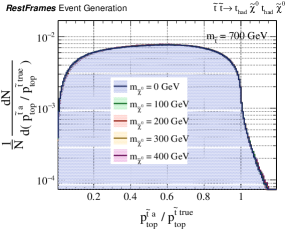
  1. 1.

    Apply the invisible mass JR VI.1, choosing MIsuperscriptsubscript𝑀IabsentM_{\footnotesize\mathrm{{\color[rgb]{0.12,0.3,0.17}\definecolor[named]{pgfstrokecolor}{rgb}{0.12,0.3,0.17}\textbf{I}}}}^{\footnotesize\leavevmode\nobreak\ } as the smallest possible quantity consistent with JR VI.3 and non-tachyonic neutralinos.

  2. 2.

    Apply the invisible rapidity JR V.1,
    choosing pI,zlabsuperscriptsubscript𝑝I𝑧labp_{\footnotesize\mathrm{{\color[rgb]{0.12,0.3,0.17}\definecolor[named]{pgfstrokecolor}{rgb}{0.12,0.3,0.17}\textbf{I}}},z}^{\footnotesize\leavevmode\nobreak\ \mathrm{\textbf{lab}}} using the tops V.

  3. 3.

    Apply the contra-boost invariant JR VI.3,
    specifying the neutralino four vectors
    using the constraint Mta=Mtbsuperscriptsubscript𝑀subscript𝑡𝑎absentsuperscriptsubscript𝑀subscript𝑡𝑏absentM_{\footnotesize\mathrm{{\color[rgb]{0.45,0.0,0.09}\definecolor[named]{pgfstrokecolor}{rgb}{0.45,0.0,0.09}\textbf{$t_{a}$}}}}^{\footnotesize\leavevmode\nobreak\ }=M_{\footnotesize\mathrm{{\color[rgb]{0.45,0.0,0.09}\definecolor[named]{pgfstrokecolor}{rgb}{0.45,0.0,0.09}\textbf{$t_{b}$}}}}^{\footnotesize\leavevmode\nobreak\ }.

Refer to caption
Figure 14: The distribution of the reconstructed top momentum in the approximation of its production frame, normalized by the true value, in simulated t~t~(tχ10)(tχ10)~𝑡~𝑡𝑡superscriptsubscript𝜒10𝑡superscriptsubscript𝜒10\tilde{t}\tilde{t}\rightarrow(t\chi_{1}^{0})(t\chi_{1}^{0}) events with varying choices of mχ~0superscriptsubscript𝑚superscript~𝜒0absentm_{\footnotesize\mathrm{{\color[rgb]{0.12,0.3,0.17}\definecolor[named]{pgfstrokecolor}{rgb}{0.12,0.3,0.17}\textbf{$\tilde{\chi}^{0}$}}}}^{\footnotesize\leavevmode\nobreak\ }.

With these choices for resolving the neutralino-related unknowns in the event, the phenomenology of the resulting estimators is studied in simulated t~t~(tχ10)(tχ10)~𝑡~𝑡𝑡superscriptsubscript𝜒10𝑡superscriptsubscript𝜒10\tilde{t}\tilde{t}\rightarrow(t\chi_{1}^{0})(t\chi_{1}^{0}) events, for various values of mχ~0superscriptsubscript𝑚superscript~𝜒0absentm_{\footnotesize\mathrm{{\color[rgb]{0.12,0.3,0.17}\definecolor[named]{pgfstrokecolor}{rgb}{0.12,0.3,0.17}\textbf{$\tilde{\chi}^{0}$}}}}^{\footnotesize\leavevmode\nobreak\ }. The distribution of the reconstructed top’s momentum in the approximation of its production frame, ptat~asuperscriptsubscript𝑝subscript𝑡𝑎subscript~𝑡𝑎p_{\footnotesize\mathrm{{\color[rgb]{0.1,0.1,0.44}\definecolor[named]{pgfstrokecolor}{rgb}{0.1,0.1,0.44}\textbf{$t_{a}$}}}}^{\footnotesize\leavevmode\nobreak\ \mathrm{{\color[rgb]{0.45,0.0,0.09}\definecolor[named]{pgfstrokecolor}{rgb}{0.45,0.0,0.09}\textbf{$\tilde{t}_{a}$}}}}, is shown in Fig. 14 for simulated events. The estimator for ptat~asuperscriptsubscript𝑝subscript𝑡𝑎subscript~𝑡𝑎p_{\footnotesize\mathrm{{\color[rgb]{0.1,0.1,0.44}\definecolor[named]{pgfstrokecolor}{rgb}{0.1,0.1,0.44}\textbf{$t_{a}$}}}}^{\footnotesize\leavevmode\nobreak\ \mathrm{{\color[rgb]{0.45,0.0,0.09}\definecolor[named]{pgfstrokecolor}{rgb}{0.45,0.0,0.09}\textbf{$\tilde{t}_{a}$}}}} exhibits no visible dependence on mχ~0superscriptsubscript𝑚superscript~𝜒0absentm_{\footnotesize\mathrm{{\color[rgb]{0.12,0.3,0.17}\definecolor[named]{pgfstrokecolor}{rgb}{0.12,0.3,0.17}\textbf{$\tilde{\chi}^{0}$}}}}^{\footnotesize\leavevmode\nobreak\ }, reliably providing sensitivity to the true value with a kinematic edge. While the estimators for the individual neutralino masses may take non-zero values, it has a negligible effect on the determination of the velocities relating the reconstructed reference frames.
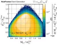
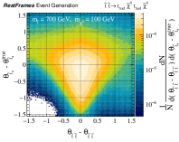
Refer to caption
Refer to caption
Figure 15: (a) Distribution of the reconstructed top momentum in the approximation of its production frame as a function of the estimated di-stop invariant mass. (b) Distribution of the di-stop decay angle, θt~t~subscript𝜃~𝑡~𝑡\theta_{\mathrm{{\color[rgb]{0.45,0.0,0.09}\definecolor[named]{pgfstrokecolor}{rgb}{0.45,0.0,0.09}\textbf{$\tilde{t}\tilde{t}$}}}}, as a function of the stop decay angle, θt~asubscript𝜃subscript~𝑡𝑎\theta_{\mathrm{{\color[rgb]{0.45,0.0,0.09}\definecolor[named]{pgfstrokecolor}{rgb}{0.45,0.0,0.09}\textbf{$\tilde{t}_{a}$}}}}. All observables are normalized appropriately by the true values of the quantities they are estimating, with angles in units radian.

As was the case for the W𝑊W mass estimator in the previous example, ptat~asuperscriptsubscript𝑝subscript𝑡𝑎subscript~𝑡𝑎p_{\footnotesize\mathrm{{\color[rgb]{0.1,0.1,0.44}\definecolor[named]{pgfstrokecolor}{rgb}{0.1,0.1,0.44}\textbf{$t_{a}$}}}}^{\footnotesize\leavevmode\nobreak\ \mathrm{{\color[rgb]{0.45,0.0,0.09}\definecolor[named]{pgfstrokecolor}{rgb}{0.45,0.0,0.09}\textbf{$\tilde{t}_{a}$}}}} (which is effectively an estimator of the stop/neutralino mass difference) can be estimated independently of Mt~t~superscriptsubscript𝑀~𝑡~𝑡absentM_{\footnotesize\mathrm{{\color[rgb]{0.45,0.0,0.09}\definecolor[named]{pgfstrokecolor}{rgb}{0.45,0.0,0.09}\textbf{$\tilde{t}\tilde{t}$}}}}^{\footnotesize\leavevmode\nobreak\ }, as demonstrated in Fig. 15(a). Similarly, the decay angles of the intermediate particle states can be measured, with their distributions for reconstructed events shown in Fig. 15(b). In particular, the decay angle of the di-stop system can be measured with excellent resolution.

VI.3 χ~20χ~20Z()χ~10h(γγ)χ~10subscriptsuperscript~𝜒02subscriptsuperscript~𝜒02𝑍subscriptsuperscript~𝜒01𝛾𝛾subscriptsuperscript~𝜒01\tilde{\chi}^{0}_{2}\tilde{\chi}^{0}_{2}\rightarrow Z(\ell\ell)\tilde{\chi}^{0}_{1}h(\gamma\gamma)\tilde{\chi}^{0}_{1} at a hadron collider

We conclude our discussion of decay topologies with two visible and two invisible particles in the final state by considering the example of neutralino, χ~20subscriptsuperscript~𝜒02\tilde{\chi}^{0}_{2}, pair production at a hadron collider, where the second neutralino mass eigenstates each decay to a lighter neutralino, χ~10subscriptsuperscript~𝜒01\tilde{\chi}^{0}_{1}, and a boson, either a Z𝑍Z or Higgs (with mh125similar-tosubscript𝑚125m_{h}\sim 125 GeV). The two final state bosons each decay to a pair of visible particles which we assume have been identified and reconstructed in the detector, with Z+𝑍superscriptsuperscriptZ\rightarrow\ell^{+}\ell^{-} and hγγ𝛾𝛾h\rightarrow\gamma\gamma. The decay tree for analyzing this final state is shown in Fig. 16.
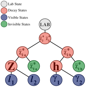
Refer to caption
Figure 16: The decay tree for analyzing χ~20χ~20Z(+)χ~10h(γγ)χ~10\tilde{\chi}_{2}^{0}\tilde{\chi}_{2}^{0}\rightarrow Z(\ell^{+}\ell^{-})\tilde{\chi}_{1}^{0}h(\rightarrow\gamma\gamma)\tilde{\chi}_{1}^{0} events. The two χ~20superscriptsubscript~𝜒20\tilde{\chi}_{2}^{0}’s are expected to be produced non-resonantly and each proceeds through two intermediate resonances of differing mass with different decay products. The two final state χ~10superscriptsubscript~𝜒10\tilde{\chi}_{1}^{0} particles are potentially massive.

The similarity of this decay topology to the previous two examples (Fig. 9 and 13) is clear; a pair of massive particles, produced resonantly or non-resonantly, each decay to a visible system of particles and an invisible system. The fact that our two visible particles, the Higgs and Z𝑍Z bosons, themselves decay to a pair of measured particles is immaterial to the strategy for choosing missing information associated with the invisible particles in the event, as we can analyze the event as a function of the measured four vectors, 𝐩Zlab=𝐩1lab+𝐩2labsuperscriptsubscript𝐩𝑍labsuperscriptsubscript𝐩subscript1labsuperscriptsubscript𝐩subscript2lab\mathbf{p}_{\footnotesize\mathrm{{\color[rgb]{0.1,0.1,0.44}\definecolor[named]{pgfstrokecolor}{rgb}{0.1,0.1,0.44}\textbf{$Z$}}}}^{\footnotesize\leavevmode\nobreak\ \mathrm{\textbf{lab}}}=\mathbf{p}_{\footnotesize\mathrm{{\color[rgb]{0.1,0.1,0.44}\definecolor[named]{pgfstrokecolor}{rgb}{0.1,0.1,0.44}\textbf{$\ell_{1}$}}}}^{\footnotesize\leavevmode\nobreak\ \mathrm{\textbf{lab}}}+\mathbf{p}_{\footnotesize\mathrm{{\color[rgb]{0.1,0.1,0.44}\definecolor[named]{pgfstrokecolor}{rgb}{0.1,0.1,0.44}\textbf{$\ell_{2}$}}}}^{\footnotesize\leavevmode\nobreak\ \mathrm{\textbf{lab}}} and 𝐩hlab=𝐩γ1lab+𝐩γ2labsuperscriptsubscript𝐩labsuperscriptsubscript𝐩subscript𝛾1labsuperscriptsubscript𝐩subscript𝛾2lab\mathbf{p}_{\footnotesize\mathrm{{\color[rgb]{0.1,0.1,0.44}\definecolor[named]{pgfstrokecolor}{rgb}{0.1,0.1,0.44}\textbf{$h$}}}}^{\footnotesize\leavevmode\nobreak\ \mathrm{\textbf{lab}}}=\mathbf{p}_{\footnotesize\mathrm{{\color[rgb]{0.1,0.1,0.44}\definecolor[named]{pgfstrokecolor}{rgb}{0.1,0.1,0.44}\textbf{$\gamma_{1}$}}}}^{\footnotesize\leavevmode\nobreak\ \mathrm{\textbf{lab}}}+\mathbf{p}_{\footnotesize\mathrm{{\color[rgb]{0.1,0.1,0.44}\definecolor[named]{pgfstrokecolor}{rgb}{0.1,0.1,0.44}\textbf{$\gamma_{2}$}}}}^{\footnotesize\leavevmode\nobreak\ \mathrm{\textbf{lab}}}, using the same JR’s as in the previous example from Section VI.2.

The important distinction in this example is that not only are our visible states, Z𝑍Z and hh, massive, but their masses are distinctly different by a non-negligible amount, adding an asymmetry to the kinematics of the event. Defining I={χ~1a,χ~1b}Isubscript~𝜒1𝑎subscript~𝜒1𝑏\mathrm{{\color[rgb]{0.12,0.3,0.17}\definecolor[named]{pgfstrokecolor}{rgb}{0.12,0.3,0.17}\textbf{I}}}=\{\mathrm{{\color[rgb]{0.12,0.3,0.17}\definecolor[named]{pgfstrokecolor}{rgb}{0.12,0.3,0.17}\textbf{$\tilde{\chi}_{1a}$}}},\mathrm{{\color[rgb]{0.12,0.3,0.17}\definecolor[named]{pgfstrokecolor}{rgb}{0.12,0.3,0.17}\textbf{$\tilde{\chi}_{1b}$}}}\} to be the collection of the invisible final state particles in the event, we interpret the measured ETmisssuperscriptsubscript𝐸𝑇miss\vec{E}_{T}^{\rm miss}  as the transverse momentum of the I system, and further define V={1,2,γ1,γ2}Vsubscript1subscript2subscript𝛾1subscript𝛾2\mathrm{{\color[rgb]{0.1,0.1,0.44}\definecolor[named]{pgfstrokecolor}{rgb}{0.1,0.1,0.44}\textbf{V}}}=\{\mathrm{{\color[rgb]{0.1,0.1,0.44}\definecolor[named]{pgfstrokecolor}{rgb}{0.1,0.1,0.44}\textbf{$\ell_{1}$}}},\mathrm{{\color[rgb]{0.1,0.1,0.44}\definecolor[named]{pgfstrokecolor}{rgb}{0.1,0.1,0.44}\textbf{$\ell_{2}$}}},\mathrm{{\color[rgb]{0.1,0.1,0.44}\definecolor[named]{pgfstrokecolor}{rgb}{0.1,0.1,0.44}\textbf{$\gamma_{1}$}}},\mathrm{{\color[rgb]{0.1,0.1,0.44}\definecolor[named]{pgfstrokecolor}{rgb}{0.1,0.1,0.44}\textbf{$\gamma_{2}$}}}\} to be the collection of all the visible particles in the final state. Choosing the unknown degrees of freedom describing how the total I system momentum is shared between the two neutralinos using the contra-boost invariant JR VI.3, we find that our estimators for Mχ~1a/bsuperscriptsubscript𝑀subscript~𝜒1𝑎𝑏absentM_{\footnotesize\mathrm{{\color[rgb]{0.12,0.3,0.17}\definecolor[named]{pgfstrokecolor}{rgb}{0.12,0.3,0.17}\textbf{$\tilde{\chi}_{1a/b}$}}}}^{\footnotesize\leavevmode\nobreak\ } are non-zero, even if we prefer they are always zero. If we choose the parameters of the JR to make these masses as small as possible, while ensuring they remain non-negative, we find that

Mχ~1a 2superscriptsubscript𝑀subscript~𝜒1𝑎2\displaystyle M_{\footnotesize\mathrm{{\color[rgb]{0.12,0.3,0.17}\definecolor[named]{pgfstrokecolor}{rgb}{0.12,0.3,0.17}\textbf{$\tilde{\chi}_{1a}$}}}}^{\footnotesize\leavevmode\nobreak\ 2} =\displaystyle= Mχ~1b 2+(mh 2mZ 2)14mZ 2(EVcm)2superscriptsubscript𝑀subscript~𝜒1𝑏2superscriptsubscript𝑚2superscriptsubscript𝑚𝑍214superscriptsubscript𝑚𝑍2superscriptsuperscriptsubscript𝐸Vcm2\displaystyle M_{\footnotesize\mathrm{{\color[rgb]{0.12,0.3,0.17}\definecolor[named]{pgfstrokecolor}{rgb}{0.12,0.3,0.17}\textbf{$\tilde{\chi}_{1b}$}}}}^{\footnotesize\leavevmode\nobreak\ 2}+(m_{\footnotesize\mathrm{{\color[rgb]{0.1,0.1,0.44}\definecolor[named]{pgfstrokecolor}{rgb}{0.1,0.1,0.44}\textbf{$h$}}}}^{\footnotesize\leavevmode\nobreak\ 2}-m_{\footnotesize\mathrm{{\color[rgb]{0.1,0.1,0.44}\definecolor[named]{pgfstrokecolor}{rgb}{0.1,0.1,0.44}\textbf{$Z$}}}}^{\footnotesize\leavevmode\nobreak\ 2})\sqrt{1-\frac{4m_{\footnotesize\mathrm{{\color[rgb]{0.1,0.1,0.44}\definecolor[named]{pgfstrokecolor}{rgb}{0.1,0.1,0.44}\textbf{$Z$}}}}^{\footnotesize\leavevmode\nobreak\ 2}}{(E_{\footnotesize\mathrm{{\color[rgb]{0.1,0.1,0.44}\definecolor[named]{pgfstrokecolor}{rgb}{0.1,0.1,0.44}\textbf{V}}}}^{\footnotesize\leavevmode\nobreak\ \mathrm{{\color[rgb]{0.45,0.0,0.09}\definecolor[named]{pgfstrokecolor}{rgb}{0.45,0.0,0.09}\textbf{cm}}}})^{2}}}
Mχ~1b 2superscriptsubscript𝑀subscript~𝜒1𝑏2\displaystyle M_{\footnotesize\mathrm{{\color[rgb]{0.12,0.3,0.17}\definecolor[named]{pgfstrokecolor}{rgb}{0.12,0.3,0.17}\textbf{$\tilde{\chi}_{1b}$}}}}^{\footnotesize\leavevmode\nobreak\ 2} =\displaystyle= mZ 2|pZcmphcm|2(EZcm+Ehcm)2superscriptsubscript𝑚𝑍2superscriptsuperscriptsubscript𝑝𝑍cmsuperscriptsubscript𝑝cm2superscriptsuperscriptsubscript𝐸𝑍cmsuperscriptsubscript𝐸cm2\displaystyle m_{\footnotesize\mathrm{{\color[rgb]{0.1,0.1,0.44}\definecolor[named]{pgfstrokecolor}{rgb}{0.1,0.1,0.44}\textbf{$Z$}}}}^{\footnotesize\leavevmode\nobreak\ 2}\frac{|\vec{p}_{\footnotesize\mathrm{{\color[rgb]{0.1,0.1,0.44}\definecolor[named]{pgfstrokecolor}{rgb}{0.1,0.1,0.44}\textbf{$Z$}}}}^{\footnotesize\leavevmode\nobreak\ \mathrm{{\color[rgb]{0.45,0.0,0.09}\definecolor[named]{pgfstrokecolor}{rgb}{0.45,0.0,0.09}\textbf{cm}}}}-\vec{p}_{\footnotesize\mathrm{{\color[rgb]{0.1,0.1,0.44}\definecolor[named]{pgfstrokecolor}{rgb}{0.1,0.1,0.44}\textbf{$h$}}}}^{\footnotesize\leavevmode\nobreak\ \mathrm{{\color[rgb]{0.45,0.0,0.09}\definecolor[named]{pgfstrokecolor}{rgb}{0.45,0.0,0.09}\textbf{cm}}}}|^{2}}{(E_{\footnotesize\mathrm{{\color[rgb]{0.1,0.1,0.44}\definecolor[named]{pgfstrokecolor}{rgb}{0.1,0.1,0.44}\textbf{$Z$}}}}^{\footnotesize\leavevmode\nobreak\ \mathrm{{\color[rgb]{0.45,0.0,0.09}\definecolor[named]{pgfstrokecolor}{rgb}{0.45,0.0,0.09}\textbf{cm}}}}+E_{\footnotesize\mathrm{{\color[rgb]{0.1,0.1,0.44}\definecolor[named]{pgfstrokecolor}{rgb}{0.1,0.1,0.44}\textbf{$h$}}}}^{\footnotesize\leavevmode\nobreak\ \mathrm{{\color[rgb]{0.45,0.0,0.09}\definecolor[named]{pgfstrokecolor}{rgb}{0.45,0.0,0.09}\textbf{cm}}}})^{2}}
+\displaystyle+ 12(mh 2mZ 2)[114mZ 2(EVcm)2],12superscriptsubscript𝑚2superscriptsubscript𝑚𝑍2delimited-[]114superscriptsubscript𝑚𝑍2superscriptsuperscriptsubscript𝐸Vcm2\displaystyle\frac{1}{2}(m_{\footnotesize\mathrm{{\color[rgb]{0.1,0.1,0.44}\definecolor[named]{pgfstrokecolor}{rgb}{0.1,0.1,0.44}\textbf{$h$}}}}^{\footnotesize\leavevmode\nobreak\ 2}-m_{\footnotesize\mathrm{{\color[rgb]{0.1,0.1,0.44}\definecolor[named]{pgfstrokecolor}{rgb}{0.1,0.1,0.44}\textbf{$Z$}}}}^{\footnotesize\leavevmode\nobreak\ 2})\left[1-\sqrt{1-\frac{4m_{\footnotesize\mathrm{{\color[rgb]{0.1,0.1,0.44}\definecolor[named]{pgfstrokecolor}{rgb}{0.1,0.1,0.44}\textbf{$Z$}}}}^{\footnotesize\leavevmode\nobreak\ 2}}{(E_{\footnotesize\mathrm{{\color[rgb]{0.1,0.1,0.44}\definecolor[named]{pgfstrokecolor}{rgb}{0.1,0.1,0.44}\textbf{V}}}}^{\footnotesize\leavevmode\nobreak\ \mathrm{{\color[rgb]{0.45,0.0,0.09}\definecolor[named]{pgfstrokecolor}{rgb}{0.45,0.0,0.09}\textbf{cm}}}})^{2}}}\right]\leavevmode\nobreak\ ,

where cm={V,I}cmVI\mathrm{{\color[rgb]{0.45,0.0,0.09}\definecolor[named]{pgfstrokecolor}{rgb}{0.45,0.0,0.09}\textbf{cm}}}=\{\mathrm{{\color[rgb]{0.1,0.1,0.44}\definecolor[named]{pgfstrokecolor}{rgb}{0.1,0.1,0.44}\textbf{V}}},\mathrm{{\color[rgb]{0.12,0.3,0.17}\definecolor[named]{pgfstrokecolor}{rgb}{0.12,0.3,0.17}\textbf{I}}}\leavevmode\nobreak\ \} denotes the center-of-mass frame of the interaction and we have assumed mhmZsuperscriptsubscript𝑚absentsuperscriptsubscript𝑚𝑍absentm_{\footnotesize\mathrm{{\color[rgb]{0.1,0.1,0.44}\definecolor[named]{pgfstrokecolor}{rgb}{0.1,0.1,0.44}\textbf{$h$}}}}^{\footnotesize\leavevmode\nobreak\ }\geq m_{\footnotesize\mathrm{{\color[rgb]{0.1,0.1,0.44}\definecolor[named]{pgfstrokecolor}{rgb}{0.1,0.1,0.44}\textbf{$Z$}}}}^{\footnotesize\leavevmode\nobreak\ }. Compared to Eq. 25 in the previous example, the expression for Mχ~1bsuperscriptsubscript𝑀subscript~𝜒1𝑏absentM_{\footnotesize\mathrm{{\color[rgb]{0.12,0.3,0.17}\definecolor[named]{pgfstrokecolor}{rgb}{0.12,0.3,0.17}\textbf{$\tilde{\chi}_{1b}$}}}}^{\footnotesize\leavevmode\nobreak\ } in Eq. VI.3 has an additional term proportional to mh 2mZ 2superscriptsubscript𝑚2superscriptsubscript𝑚𝑍2m_{\footnotesize\mathrm{{\color[rgb]{0.1,0.1,0.44}\definecolor[named]{pgfstrokecolor}{rgb}{0.1,0.1,0.44}\textbf{$h$}}}}^{\footnotesize\leavevmode\nobreak\ 2}-m_{\footnotesize\mathrm{{\color[rgb]{0.1,0.1,0.44}\definecolor[named]{pgfstrokecolor}{rgb}{0.1,0.1,0.44}\textbf{$Z$}}}}^{\footnotesize\leavevmode\nobreak\ 2}, implying that differences in the visible particle masses are additionally absorbed into the invisible particle masses. More concerning is that Mχ~1asuperscriptsubscript𝑀subscript~𝜒1𝑎absentM_{\footnotesize\mathrm{{\color[rgb]{0.12,0.3,0.17}\definecolor[named]{pgfstrokecolor}{rgb}{0.12,0.3,0.17}\textbf{$\tilde{\chi}_{1a}$}}}}^{\footnotesize\leavevmode\nobreak\ } is systematically larger than Mχ~1bsuperscriptsubscript𝑀subscript~𝜒1𝑏absentM_{\footnotesize\mathrm{{\color[rgb]{0.12,0.3,0.17}\definecolor[named]{pgfstrokecolor}{rgb}{0.12,0.3,0.17}\textbf{$\tilde{\chi}_{1b}$}}}}^{\footnotesize\leavevmode\nobreak\ }, where Eq. VI.3 implies

Mχ~1a 2Mχ~1b 2(mhmZ)32(mh+3mZ)12.superscriptsubscript𝑀subscript~𝜒1𝑎2superscriptsubscript𝑀subscript~𝜒1𝑏2superscriptsuperscriptsubscript𝑚absentsuperscriptsubscript𝑚𝑍absent32superscriptsuperscriptsubscript𝑚absent3superscriptsubscript𝑚𝑍absent12\displaystyle M_{\footnotesize\mathrm{{\color[rgb]{0.12,0.3,0.17}\definecolor[named]{pgfstrokecolor}{rgb}{0.12,0.3,0.17}\textbf{$\tilde{\chi}_{1a}$}}}}^{\footnotesize\leavevmode\nobreak\ 2}-M_{\footnotesize\mathrm{{\color[rgb]{0.12,0.3,0.17}\definecolor[named]{pgfstrokecolor}{rgb}{0.12,0.3,0.17}\textbf{$\tilde{\chi}_{1b}$}}}}^{\footnotesize\leavevmode\nobreak\ 2}\geq(m_{\footnotesize\mathrm{{\color[rgb]{0.1,0.1,0.44}\definecolor[named]{pgfstrokecolor}{rgb}{0.1,0.1,0.44}\textbf{$h$}}}}^{\footnotesize\leavevmode\nobreak\ }-m_{\footnotesize\mathrm{{\color[rgb]{0.1,0.1,0.44}\definecolor[named]{pgfstrokecolor}{rgb}{0.1,0.1,0.44}\textbf{$Z$}}}}^{\footnotesize\leavevmode\nobreak\ })^{\frac{3}{2}}(m_{\footnotesize\mathrm{{\color[rgb]{0.1,0.1,0.44}\definecolor[named]{pgfstrokecolor}{rgb}{0.1,0.1,0.44}\textbf{$h$}}}}^{\footnotesize\leavevmode\nobreak\ }+3m_{\footnotesize\mathrm{{\color[rgb]{0.1,0.1,0.44}\definecolor[named]{pgfstrokecolor}{rgb}{0.1,0.1,0.44}\textbf{$Z$}}}}^{\footnotesize\leavevmode\nobreak\ })^{\frac{1}{2}}\leavevmode\nobreak\ . (30)

The constraint Mχ~2a=Mχ~2bsuperscriptsubscript𝑀subscript~𝜒2𝑎absentsuperscriptsubscript𝑀subscript~𝜒2𝑏absentM_{\footnotesize\mathrm{{\color[rgb]{0.45,0.0,0.09}\definecolor[named]{pgfstrokecolor}{rgb}{0.45,0.0,0.09}\textbf{$\tilde{\chi}_{2a}$}}}}^{\footnotesize\leavevmode\nobreak\ }=M_{\footnotesize\mathrm{{\color[rgb]{0.45,0.0,0.09}\definecolor[named]{pgfstrokecolor}{rgb}{0.45,0.0,0.09}\textbf{$\tilde{\chi}_{2b}$}}}}^{\footnotesize\leavevmode\nobreak\ } associated with the contra-boost invariant JR has caused our Mχ~1a/bsuperscriptsubscript𝑀subscript~𝜒1𝑎𝑏absentM_{\footnotesize\mathrm{{\color[rgb]{0.12,0.3,0.17}\definecolor[named]{pgfstrokecolor}{rgb}{0.12,0.3,0.17}\textbf{$\tilde{\chi}_{1a/b}$}}}}^{\footnotesize\leavevmode\nobreak\ } estimators to develop a large systematic difference, a kinematic feature that is not present in the process we are hoping to study. In our case, the two lightest neutralinos have the same mass, meaning that the one associated with the Z𝑍Z decay should systematically receive more momentum from its parent’s decay rather than increase in mass itself. More generally, for lack of a better choice, a practical application would desire that both the mass estimators Mχ~1a/bsuperscriptsubscript𝑀subscript~𝜒1𝑎𝑏absentM_{\footnotesize\mathrm{{\color[rgb]{0.12,0.3,0.17}\definecolor[named]{pgfstrokecolor}{rgb}{0.12,0.3,0.17}\textbf{$\tilde{\chi}_{1a/b}$}}}}^{\footnotesize\leavevmode\nobreak\ } take values as close to zero as possible. To achieve this behavior, we reconsider how the contra-boost invariant JR we apply is constructed.

With the assumption Mχ~2a=Mχ~2bsuperscriptsubscript𝑀subscript~𝜒2𝑎absentsuperscriptsubscript𝑀subscript~𝜒2𝑏absentM_{\footnotesize\mathrm{{\color[rgb]{0.45,0.0,0.09}\definecolor[named]{pgfstrokecolor}{rgb}{0.45,0.0,0.09}\textbf{$\tilde{\chi}_{2a}$}}}}^{\footnotesize\leavevmode\nobreak\ }=M_{\footnotesize\mathrm{{\color[rgb]{0.45,0.0,0.09}\definecolor[named]{pgfstrokecolor}{rgb}{0.45,0.0,0.09}\textbf{$\tilde{\chi}_{2b}$}}}}^{\footnotesize\leavevmode\nobreak\ }, we can again relate the velocities of these two particles in their mutual center-of-mass frame by a single contra-boost, βcsubscript𝛽𝑐\vec{\beta}_{c}, and choose its value to constrain the momentum of the invisible neutralinos. Instead of setting βcsubscript𝛽𝑐\vec{\beta}_{c} according to an explicit minimization as we did in previous examples, we consider an ad-hoc generalization that maintains the contra-boost invariance of the choice:

βc=βχ~2acm=βχ~2bcm=capZcmcbphcmcaEZcm+cbEhcm,subscript𝛽𝑐superscriptsubscript𝛽subscript~𝜒2𝑎cmsuperscriptsubscript𝛽subscript~𝜒2𝑏cmsubscript𝑐𝑎superscriptsubscript𝑝𝑍cmsubscript𝑐𝑏superscriptsubscript𝑝cmsubscript𝑐𝑎superscriptsubscript𝐸𝑍cmsubscript𝑐𝑏superscriptsubscript𝐸cm\displaystyle\vec{\beta}_{c}=\vec{\beta}_{\footnotesize\mathrm{{\color[rgb]{0.45,0.0,0.09}\definecolor[named]{pgfstrokecolor}{rgb}{0.45,0.0,0.09}\textbf{$\tilde{\chi}_{2a}$}}}}^{\footnotesize\leavevmode\nobreak\ \mathrm{{\color[rgb]{0.45,0.0,0.09}\definecolor[named]{pgfstrokecolor}{rgb}{0.45,0.0,0.09}\textbf{cm}}}}=-\vec{\beta}_{\footnotesize\mathrm{{\color[rgb]{0.45,0.0,0.09}\definecolor[named]{pgfstrokecolor}{rgb}{0.45,0.0,0.09}\textbf{$\tilde{\chi}_{2b}$}}}}^{\footnotesize\leavevmode\nobreak\ \mathrm{{\color[rgb]{0.45,0.0,0.09}\definecolor[named]{pgfstrokecolor}{rgb}{0.45,0.0,0.09}\textbf{cm}}}}=\frac{c_{a}\vec{p}_{\footnotesize\mathrm{{\color[rgb]{0.1,0.1,0.44}\definecolor[named]{pgfstrokecolor}{rgb}{0.1,0.1,0.44}\textbf{$Z$}}}}^{\footnotesize\leavevmode\nobreak\ \mathrm{{\color[rgb]{0.45,0.0,0.09}\definecolor[named]{pgfstrokecolor}{rgb}{0.45,0.0,0.09}\textbf{cm}}}}-c_{b}\vec{p}_{\footnotesize\mathrm{{\color[rgb]{0.1,0.1,0.44}\definecolor[named]{pgfstrokecolor}{rgb}{0.1,0.1,0.44}\textbf{$h$}}}}^{\footnotesize\leavevmode\nobreak\ \mathrm{{\color[rgb]{0.45,0.0,0.09}\definecolor[named]{pgfstrokecolor}{rgb}{0.45,0.0,0.09}\textbf{cm}}}}}{c_{a}E_{\footnotesize\mathrm{{\color[rgb]{0.1,0.1,0.44}\definecolor[named]{pgfstrokecolor}{rgb}{0.1,0.1,0.44}\textbf{$Z$}}}}^{\footnotesize\leavevmode\nobreak\ \mathrm{{\color[rgb]{0.45,0.0,0.09}\definecolor[named]{pgfstrokecolor}{rgb}{0.45,0.0,0.09}\textbf{cm}}}}+c_{b}E_{\footnotesize\mathrm{{\color[rgb]{0.1,0.1,0.44}\definecolor[named]{pgfstrokecolor}{rgb}{0.1,0.1,0.44}\textbf{$h$}}}}^{\footnotesize\leavevmode\nobreak\ \mathrm{{\color[rgb]{0.45,0.0,0.09}\definecolor[named]{pgfstrokecolor}{rgb}{0.45,0.0,0.09}\textbf{cm}}}}}\leavevmode\nobreak\ , (31)

where casubscript𝑐𝑎c_{a} and cbsubscript𝑐𝑏c_{b} are unspecified functions of the visible four vectors in the interaction center-of-mass frame, cm. With this choice, the reconstructed energies of the visible particles in their respective production frames can be expressed as

EZχ~2asuperscriptsubscript𝐸𝑍subscript~𝜒2𝑎\displaystyle E_{\footnotesize\mathrm{{\color[rgb]{0.1,0.1,0.44}\definecolor[named]{pgfstrokecolor}{rgb}{0.1,0.1,0.44}\textbf{$Z$}}}}^{\footnotesize\leavevmode\nobreak\ \mathrm{{\color[rgb]{0.45,0.0,0.09}\definecolor[named]{pgfstrokecolor}{rgb}{0.45,0.0,0.09}\textbf{$\tilde{\chi}_{2a}$}}}} =\displaystyle= camZ 2+(cb/2)Mc2(𝐩Zcm,𝐩hcm)ca2mZ 2+cb2mh 2+cacbMc2(𝐩Zcm,𝐩hcm)subscript𝑐𝑎superscriptsubscript𝑚𝑍2subscript𝑐𝑏2superscriptsubscript𝑀𝑐2superscriptsubscript𝐩𝑍cmsuperscriptsubscript𝐩cmsuperscriptsubscript𝑐𝑎2superscriptsubscript𝑚𝑍2superscriptsubscript𝑐𝑏2superscriptsubscript𝑚2subscript𝑐𝑎subscript𝑐𝑏superscriptsubscript𝑀𝑐2superscriptsubscript𝐩𝑍cmsuperscriptsubscript𝐩cm\displaystyle\frac{c_{a}m_{\footnotesize\mathrm{{\color[rgb]{0.1,0.1,0.44}\definecolor[named]{pgfstrokecolor}{rgb}{0.1,0.1,0.44}\textbf{$Z$}}}}^{\footnotesize\leavevmode\nobreak\ 2}+(c_{b}/2)M_{c}^{2}(\mathbf{p}_{\footnotesize\mathrm{{\color[rgb]{0.1,0.1,0.44}\definecolor[named]{pgfstrokecolor}{rgb}{0.1,0.1,0.44}\textbf{$Z$}}}}^{\footnotesize\leavevmode\nobreak\ \mathrm{{\color[rgb]{0.45,0.0,0.09}\definecolor[named]{pgfstrokecolor}{rgb}{0.45,0.0,0.09}\textbf{cm}}}},\mathbf{p}_{\footnotesize\mathrm{{\color[rgb]{0.1,0.1,0.44}\definecolor[named]{pgfstrokecolor}{rgb}{0.1,0.1,0.44}\textbf{$h$}}}}^{\footnotesize\leavevmode\nobreak\ \mathrm{{\color[rgb]{0.45,0.0,0.09}\definecolor[named]{pgfstrokecolor}{rgb}{0.45,0.0,0.09}\textbf{cm}}}})}{\sqrt{c_{a}^{2}m_{\footnotesize\mathrm{{\color[rgb]{0.1,0.1,0.44}\definecolor[named]{pgfstrokecolor}{rgb}{0.1,0.1,0.44}\textbf{$Z$}}}}^{\footnotesize\leavevmode\nobreak\ 2}+c_{b}^{2}m_{\footnotesize\mathrm{{\color[rgb]{0.1,0.1,0.44}\definecolor[named]{pgfstrokecolor}{rgb}{0.1,0.1,0.44}\textbf{$h$}}}}^{\footnotesize\leavevmode\nobreak\ 2}+c_{a}c_{b}M_{c}^{2}(\mathbf{p}_{\footnotesize\mathrm{{\color[rgb]{0.1,0.1,0.44}\definecolor[named]{pgfstrokecolor}{rgb}{0.1,0.1,0.44}\textbf{$Z$}}}}^{\footnotesize\leavevmode\nobreak\ \mathrm{{\color[rgb]{0.45,0.0,0.09}\definecolor[named]{pgfstrokecolor}{rgb}{0.45,0.0,0.09}\textbf{cm}}}},\mathbf{p}_{\footnotesize\mathrm{{\color[rgb]{0.1,0.1,0.44}\definecolor[named]{pgfstrokecolor}{rgb}{0.1,0.1,0.44}\textbf{$h$}}}}^{\footnotesize\leavevmode\nobreak\ \mathrm{{\color[rgb]{0.45,0.0,0.09}\definecolor[named]{pgfstrokecolor}{rgb}{0.45,0.0,0.09}\textbf{cm}}}})}} (32)
Ehχ~2bsuperscriptsubscript𝐸subscript~𝜒2𝑏\displaystyle E_{\footnotesize\mathrm{{\color[rgb]{0.1,0.1,0.44}\definecolor[named]{pgfstrokecolor}{rgb}{0.1,0.1,0.44}\textbf{$h$}}}}^{\footnotesize\leavevmode\nobreak\ \mathrm{{\color[rgb]{0.45,0.0,0.09}\definecolor[named]{pgfstrokecolor}{rgb}{0.45,0.0,0.09}\textbf{$\tilde{\chi}_{2b}$}}}} =\displaystyle= cbmh 2+(ca/2)Mc2(𝐩Zcm,𝐩hcm)ca2mZ 2+cb2mh 2+cacbMc2(𝐩Zcm,𝐩hcm).subscript𝑐𝑏superscriptsubscript𝑚2subscript𝑐𝑎2superscriptsubscript𝑀𝑐2superscriptsubscript𝐩𝑍cmsuperscriptsubscript𝐩cmsuperscriptsubscript𝑐𝑎2superscriptsubscript𝑚𝑍2superscriptsubscript𝑐𝑏2superscriptsubscript𝑚2subscript𝑐𝑎subscript𝑐𝑏superscriptsubscript𝑀𝑐2superscriptsubscript𝐩𝑍cmsuperscriptsubscript𝐩cm\displaystyle\frac{c_{b}m_{\footnotesize\mathrm{{\color[rgb]{0.1,0.1,0.44}\definecolor[named]{pgfstrokecolor}{rgb}{0.1,0.1,0.44}\textbf{$h$}}}}^{\footnotesize\leavevmode\nobreak\ 2}+(c_{a}/2)M_{c}^{2}(\mathbf{p}_{\footnotesize\mathrm{{\color[rgb]{0.1,0.1,0.44}\definecolor[named]{pgfstrokecolor}{rgb}{0.1,0.1,0.44}\textbf{$Z$}}}}^{\footnotesize\leavevmode\nobreak\ \mathrm{{\color[rgb]{0.45,0.0,0.09}\definecolor[named]{pgfstrokecolor}{rgb}{0.45,0.0,0.09}\textbf{cm}}}},\mathbf{p}_{\footnotesize\mathrm{{\color[rgb]{0.1,0.1,0.44}\definecolor[named]{pgfstrokecolor}{rgb}{0.1,0.1,0.44}\textbf{$h$}}}}^{\footnotesize\leavevmode\nobreak\ \mathrm{{\color[rgb]{0.45,0.0,0.09}\definecolor[named]{pgfstrokecolor}{rgb}{0.45,0.0,0.09}\textbf{cm}}}})}{\sqrt{c_{a}^{2}m_{\footnotesize\mathrm{{\color[rgb]{0.1,0.1,0.44}\definecolor[named]{pgfstrokecolor}{rgb}{0.1,0.1,0.44}\textbf{$Z$}}}}^{\footnotesize\leavevmode\nobreak\ 2}+c_{b}^{2}m_{\footnotesize\mathrm{{\color[rgb]{0.1,0.1,0.44}\definecolor[named]{pgfstrokecolor}{rgb}{0.1,0.1,0.44}\textbf{$h$}}}}^{\footnotesize\leavevmode\nobreak\ 2}+c_{a}c_{b}M_{c}^{2}(\mathbf{p}_{\footnotesize\mathrm{{\color[rgb]{0.1,0.1,0.44}\definecolor[named]{pgfstrokecolor}{rgb}{0.1,0.1,0.44}\textbf{$Z$}}}}^{\footnotesize\leavevmode\nobreak\ \mathrm{{\color[rgb]{0.45,0.0,0.09}\definecolor[named]{pgfstrokecolor}{rgb}{0.45,0.0,0.09}\textbf{cm}}}},\mathbf{p}_{\footnotesize\mathrm{{\color[rgb]{0.1,0.1,0.44}\definecolor[named]{pgfstrokecolor}{rgb}{0.1,0.1,0.44}\textbf{$h$}}}}^{\footnotesize\leavevmode\nobreak\ \mathrm{{\color[rgb]{0.45,0.0,0.09}\definecolor[named]{pgfstrokecolor}{rgb}{0.45,0.0,0.09}\textbf{cm}}}})}}\leavevmode\nobreak\ .

As there are only contra-boost invariant quantities appearing in Eq. 32 this means that, as long as there are also only contra-boost invariant quantities appearing in casubscript𝑐𝑎c_{a} and cbsubscript𝑐𝑏c_{b}, our estimators EZχ~2asuperscriptsubscript𝐸𝑍subscript~𝜒2𝑎E_{\footnotesize\mathrm{{\color[rgb]{0.1,0.1,0.44}\definecolor[named]{pgfstrokecolor}{rgb}{0.1,0.1,0.44}\textbf{$Z$}}}}^{\footnotesize\leavevmode\nobreak\ \mathrm{{\color[rgb]{0.45,0.0,0.09}\definecolor[named]{pgfstrokecolor}{rgb}{0.45,0.0,0.09}\textbf{$\tilde{\chi}_{2a}$}}}} and Ehχ~2bsuperscriptsubscript𝐸subscript~𝜒2𝑏E_{\footnotesize\mathrm{{\color[rgb]{0.1,0.1,0.44}\definecolor[named]{pgfstrokecolor}{rgb}{0.1,0.1,0.44}\textbf{$h$}}}}^{\footnotesize\leavevmode\nobreak\ \mathrm{{\color[rgb]{0.45,0.0,0.09}\definecolor[named]{pgfstrokecolor}{rgb}{0.45,0.0,0.09}\textbf{$\tilde{\chi}_{2b}$}}}} will exhibit this property.

Hence, there is a family of contra-boost invariant choices for βcsubscript𝛽𝑐\beta_{c}, defined by the different contra-boost invariant choices for the factors casubscript𝑐𝑎c_{a} and cbsubscript𝑐𝑏c_{b}, which can be constructed from factors like mZ 2superscriptsubscript𝑚𝑍2m_{\footnotesize\mathrm{{\color[rgb]{0.1,0.1,0.44}\definecolor[named]{pgfstrokecolor}{rgb}{0.1,0.1,0.44}\textbf{$Z$}}}}^{\footnotesize\leavevmode\nobreak\ 2}, mh 2superscriptsubscript𝑚2m_{\footnotesize\mathrm{{\color[rgb]{0.1,0.1,0.44}\definecolor[named]{pgfstrokecolor}{rgb}{0.1,0.1,0.44}\textbf{$h$}}}}^{\footnotesize\leavevmode\nobreak\ 2}, and Mc2(𝐩Zcm,𝐩hcm)superscriptsubscript𝑀𝑐2superscriptsubscript𝐩𝑍cmsuperscriptsubscript𝐩cmM_{c}^{2}(\mathbf{p}_{\footnotesize\mathrm{{\color[rgb]{0.1,0.1,0.44}\definecolor[named]{pgfstrokecolor}{rgb}{0.1,0.1,0.44}\textbf{$Z$}}}}^{\footnotesize\leavevmode\nobreak\ \mathrm{{\color[rgb]{0.45,0.0,0.09}\definecolor[named]{pgfstrokecolor}{rgb}{0.45,0.0,0.09}\textbf{cm}}}},\mathbf{p}_{\footnotesize\mathrm{{\color[rgb]{0.1,0.1,0.44}\definecolor[named]{pgfstrokecolor}{rgb}{0.1,0.1,0.44}\textbf{$h$}}}}^{\footnotesize\leavevmode\nobreak\ \mathrm{{\color[rgb]{0.45,0.0,0.09}\definecolor[named]{pgfstrokecolor}{rgb}{0.45,0.0,0.09}\textbf{cm}}}}) which have this invariance property. We would like to use the additional degree of freedom associated with this choice to mitigate the large values of the estimators of invisible particle masses seen in Eq. VI.3.

Defining

casubscript𝑐𝑎\displaystyle c_{a} =\displaystyle= 12(1+k^ka)121^𝑘subscript𝑘𝑎\displaystyle\frac{1}{2}\left(1+\hat{k}k_{a}\right) (33)
cbsubscript𝑐𝑏\displaystyle c_{b} =\displaystyle= 12(1+k^kb),121^𝑘subscript𝑘𝑏\displaystyle\frac{1}{2}\left(1+\hat{k}k_{b}\right)\leavevmode\nobreak\ ,

the mass-squared difference of our estimators Mχ~1a/bsuperscriptsubscript𝑀subscript~𝜒1𝑎𝑏absentM_{\footnotesize\mathrm{{\color[rgb]{0.12,0.3,0.17}\definecolor[named]{pgfstrokecolor}{rgb}{0.12,0.3,0.17}\textbf{$\tilde{\chi}_{1a/b}$}}}}^{\footnotesize\leavevmode\nobreak\ }, using the more general contra-boost of Eq. 31, can be expressed as

ΔMχ~1 2Mχ~1a 2Mχ~1b 2=Δsuperscriptsubscript𝑀subscript~𝜒12superscriptsubscript𝑀subscript~𝜒1𝑎2superscriptsubscript𝑀subscript~𝜒1𝑏2absent\displaystyle\Delta M_{\footnotesize\mathrm{{\color[rgb]{0.12,0.3,0.17}\definecolor[named]{pgfstrokecolor}{rgb}{0.12,0.3,0.17}\textbf{$\tilde{\chi}_{1}$}}}}^{\footnotesize\leavevmode\nobreak\ 2}\equiv M_{\footnotesize\mathrm{{\color[rgb]{0.12,0.3,0.17}\definecolor[named]{pgfstrokecolor}{rgb}{0.12,0.3,0.17}\textbf{$\tilde{\chi}_{1a}$}}}}^{\footnotesize\leavevmode\nobreak\ 2}-M_{\footnotesize\mathrm{{\color[rgb]{0.12,0.3,0.17}\definecolor[named]{pgfstrokecolor}{rgb}{0.12,0.3,0.17}\textbf{$\tilde{\chi}_{1b}$}}}}^{\footnotesize\leavevmode\nobreak\ 2}= (34)
k^[(kakb)Mc2(𝐩Zcm,𝐩hcm)/2(kamZ 2kbmh 2)].^𝑘delimited-[]subscript𝑘𝑎subscript𝑘𝑏superscriptsubscript𝑀𝑐2superscriptsubscript𝐩𝑍cmsuperscriptsubscript𝐩cm2subscript𝑘𝑎superscriptsubscript𝑚𝑍2subscript𝑘𝑏superscriptsubscript𝑚2\displaystyle\hat{k}\left[(k_{a}-k_{b})M_{c}^{2}(\mathbf{p}_{\footnotesize\mathrm{{\color[rgb]{0.1,0.1,0.44}\definecolor[named]{pgfstrokecolor}{rgb}{0.1,0.1,0.44}\textbf{$Z$}}}}^{\footnotesize\leavevmode\nobreak\ \mathrm{{\color[rgb]{0.45,0.0,0.09}\definecolor[named]{pgfstrokecolor}{rgb}{0.45,0.0,0.09}\textbf{cm}}}},\mathbf{p}_{\footnotesize\mathrm{{\color[rgb]{0.1,0.1,0.44}\definecolor[named]{pgfstrokecolor}{rgb}{0.1,0.1,0.44}\textbf{$h$}}}}^{\footnotesize\leavevmode\nobreak\ \mathrm{{\color[rgb]{0.45,0.0,0.09}\definecolor[named]{pgfstrokecolor}{rgb}{0.45,0.0,0.09}\textbf{cm}}}})/2-(k_{a}m_{\footnotesize\mathrm{{\color[rgb]{0.1,0.1,0.44}\definecolor[named]{pgfstrokecolor}{rgb}{0.1,0.1,0.44}\textbf{$Z$}}}}^{\footnotesize\leavevmode\nobreak\ 2}-k_{b}m_{\footnotesize\mathrm{{\color[rgb]{0.1,0.1,0.44}\definecolor[named]{pgfstrokecolor}{rgb}{0.1,0.1,0.44}\textbf{$h$}}}}^{\footnotesize\leavevmode\nobreak\ 2})\right]\leavevmode\nobreak\ .

We use our choice for the factors kasubscript𝑘𝑎k_{a} and kbsubscript𝑘𝑏k_{b} to minimize ΔMχ~1 2Δsuperscriptsubscript𝑀subscript~𝜒12\Delta M_{\footnotesize\mathrm{{\color[rgb]{0.12,0.3,0.17}\definecolor[named]{pgfstrokecolor}{rgb}{0.12,0.3,0.17}\textbf{$\tilde{\chi}_{1}$}}}}^{\footnotesize\leavevmode\nobreak\ 2}, in particular ensuring that limMc2ΔMχ~1 2=0subscriptsuperscriptsubscript𝑀𝑐2Δsuperscriptsubscript𝑀subscript~𝜒120\lim_{M_{c}^{2}\rightarrow\infty}\Delta M_{\footnotesize\mathrm{{\color[rgb]{0.12,0.3,0.17}\definecolor[named]{pgfstrokecolor}{rgb}{0.12,0.3,0.17}\textbf{$\tilde{\chi}_{1}$}}}}^{\footnotesize\leavevmode\nobreak\ 2}=0, with

kasubscript𝑘𝑎\displaystyle k_{a} =\displaystyle= mZ 2mh 2+Mc2(𝐩Zcm,𝐩hcm)2mZ 2mh 2superscriptsubscript𝑚𝑍2superscriptsubscript𝑚2superscriptsubscript𝑀𝑐2superscriptsubscript𝐩𝑍cmsuperscriptsubscript𝐩cm2superscriptsubscript𝑚𝑍2superscriptsubscript𝑚2\displaystyle m_{\footnotesize\mathrm{{\color[rgb]{0.1,0.1,0.44}\definecolor[named]{pgfstrokecolor}{rgb}{0.1,0.1,0.44}\textbf{$Z$}}}}^{\footnotesize\leavevmode\nobreak\ 2}-m_{\footnotesize\mathrm{{\color[rgb]{0.1,0.1,0.44}\definecolor[named]{pgfstrokecolor}{rgb}{0.1,0.1,0.44}\textbf{$h$}}}}^{\footnotesize\leavevmode\nobreak\ 2}+M_{c}^{2}(\mathbf{p}_{\footnotesize\mathrm{{\color[rgb]{0.1,0.1,0.44}\definecolor[named]{pgfstrokecolor}{rgb}{0.1,0.1,0.44}\textbf{$Z$}}}}^{\footnotesize\leavevmode\nobreak\ \mathrm{{\color[rgb]{0.45,0.0,0.09}\definecolor[named]{pgfstrokecolor}{rgb}{0.45,0.0,0.09}\textbf{cm}}}},\mathbf{p}_{\footnotesize\mathrm{{\color[rgb]{0.1,0.1,0.44}\definecolor[named]{pgfstrokecolor}{rgb}{0.1,0.1,0.44}\textbf{$h$}}}}^{\footnotesize\leavevmode\nobreak\ \mathrm{{\color[rgb]{0.45,0.0,0.09}\definecolor[named]{pgfstrokecolor}{rgb}{0.45,0.0,0.09}\textbf{cm}}}})-2m_{\footnotesize\mathrm{{\color[rgb]{0.1,0.1,0.44}\definecolor[named]{pgfstrokecolor}{rgb}{0.1,0.1,0.44}\textbf{$Z$}}}}^{\footnotesize\leavevmode\nobreak\ 2}m_{\footnotesize\mathrm{{\color[rgb]{0.1,0.1,0.44}\definecolor[named]{pgfstrokecolor}{rgb}{0.1,0.1,0.44}\textbf{$h$}}}}^{\footnotesize\leavevmode\nobreak\ 2} (35)
kbsubscript𝑘𝑏\displaystyle k_{b} =\displaystyle= mh 2mZ 2+Mc2(𝐩Zcm,𝐩hcm)2mZ 2mh 2,superscriptsubscript𝑚2superscriptsubscript𝑚𝑍2superscriptsubscript𝑀𝑐2superscriptsubscript𝐩𝑍cmsuperscriptsubscript𝐩cm2superscriptsubscript𝑚𝑍2superscriptsubscript𝑚2\displaystyle m_{\footnotesize\mathrm{{\color[rgb]{0.1,0.1,0.44}\definecolor[named]{pgfstrokecolor}{rgb}{0.1,0.1,0.44}\textbf{$h$}}}}^{\footnotesize\leavevmode\nobreak\ 2}-m_{\footnotesize\mathrm{{\color[rgb]{0.1,0.1,0.44}\definecolor[named]{pgfstrokecolor}{rgb}{0.1,0.1,0.44}\textbf{$Z$}}}}^{\footnotesize\leavevmode\nobreak\ 2}+M_{c}^{2}(\mathbf{p}_{\footnotesize\mathrm{{\color[rgb]{0.1,0.1,0.44}\definecolor[named]{pgfstrokecolor}{rgb}{0.1,0.1,0.44}\textbf{$Z$}}}}^{\footnotesize\leavevmode\nobreak\ \mathrm{{\color[rgb]{0.45,0.0,0.09}\definecolor[named]{pgfstrokecolor}{rgb}{0.45,0.0,0.09}\textbf{cm}}}},\mathbf{p}_{\footnotesize\mathrm{{\color[rgb]{0.1,0.1,0.44}\definecolor[named]{pgfstrokecolor}{rgb}{0.1,0.1,0.44}\textbf{$h$}}}}^{\footnotesize\leavevmode\nobreak\ \mathrm{{\color[rgb]{0.45,0.0,0.09}\definecolor[named]{pgfstrokecolor}{rgb}{0.45,0.0,0.09}\textbf{cm}}}})-2m_{\footnotesize\mathrm{{\color[rgb]{0.1,0.1,0.44}\definecolor[named]{pgfstrokecolor}{rgb}{0.1,0.1,0.44}\textbf{$Z$}}}}^{\footnotesize\leavevmode\nobreak\ 2}m_{\footnotesize\mathrm{{\color[rgb]{0.1,0.1,0.44}\definecolor[named]{pgfstrokecolor}{rgb}{0.1,0.1,0.44}\textbf{$h$}}}}^{\footnotesize\leavevmode\nobreak\ 2}\leavevmode\nobreak\ ,

which results in

ΔMχ~1 2=k^(mh+mZ)(mhmZ)3.Δsuperscriptsubscript𝑀subscript~𝜒12^𝑘superscriptsubscript𝑚absentsuperscriptsubscript𝑚𝑍absentsuperscriptsuperscriptsubscript𝑚absentsuperscriptsubscript𝑚𝑍absent3\displaystyle\Delta M_{\footnotesize\mathrm{{\color[rgb]{0.12,0.3,0.17}\definecolor[named]{pgfstrokecolor}{rgb}{0.12,0.3,0.17}\textbf{$\tilde{\chi}_{1}$}}}}^{\footnotesize\leavevmode\nobreak\ 2}=\hat{k}(m_{\footnotesize\mathrm{{\color[rgb]{0.1,0.1,0.44}\definecolor[named]{pgfstrokecolor}{rgb}{0.1,0.1,0.44}\textbf{$h$}}}}^{\footnotesize\leavevmode\nobreak\ }+m_{\footnotesize\mathrm{{\color[rgb]{0.1,0.1,0.44}\definecolor[named]{pgfstrokecolor}{rgb}{0.1,0.1,0.44}\textbf{$Z$}}}}^{\footnotesize\leavevmode\nobreak\ })(m_{\footnotesize\mathrm{{\color[rgb]{0.1,0.1,0.44}\definecolor[named]{pgfstrokecolor}{rgb}{0.1,0.1,0.44}\textbf{$h$}}}}^{\footnotesize\leavevmode\nobreak\ }-m_{\footnotesize\mathrm{{\color[rgb]{0.1,0.1,0.44}\definecolor[named]{pgfstrokecolor}{rgb}{0.1,0.1,0.44}\textbf{$Z$}}}}^{\footnotesize\leavevmode\nobreak\ })^{3}\leavevmode\nobreak\ . (36)

The factor k^^𝑘\hat{k} effectively normalizes kasubscript𝑘𝑎k_{a} and kbsubscript𝑘𝑏k_{b} to be dimensionless, and with limMc2k^1=Mc2(𝐩Zcm,𝐩hcm)subscriptsuperscriptsubscript𝑀𝑐2superscript^𝑘1superscriptsubscript𝑀𝑐2superscriptsubscript𝐩𝑍cmsuperscriptsubscript𝐩cm\lim_{M_{c}^{2}\rightarrow\infty}\hat{k}^{-1}=M_{c}^{2}(\mathbf{p}_{\footnotesize\mathrm{{\color[rgb]{0.1,0.1,0.44}\definecolor[named]{pgfstrokecolor}{rgb}{0.1,0.1,0.44}\textbf{$Z$}}}}^{\footnotesize\leavevmode\nobreak\ \mathrm{{\color[rgb]{0.45,0.0,0.09}\definecolor[named]{pgfstrokecolor}{rgb}{0.45,0.0,0.09}\textbf{cm}}}},\mathbf{p}_{\footnotesize\mathrm{{\color[rgb]{0.1,0.1,0.44}\definecolor[named]{pgfstrokecolor}{rgb}{0.1,0.1,0.44}\textbf{$h$}}}}^{\footnotesize\leavevmode\nobreak\ \mathrm{{\color[rgb]{0.45,0.0,0.09}\definecolor[named]{pgfstrokecolor}{rgb}{0.45,0.0,0.09}\textbf{cm}}}}) the invisible particle mass difference will approach zero when the mass splitting between parent χ~20superscriptsubscript~𝜒20\tilde{\chi}_{2}^{0} and invisible χ~10superscriptsubscript~𝜒10\tilde{\chi}_{1}^{0} is large, relative to the Z𝑍Z and Higgs boson masses.

To see that our ultimate choice for k^^𝑘\hat{k} has the expected asymptotic behavior, we choose it’s value by setting Mχ~1b=0superscriptsubscript𝑀subscript~𝜒1𝑏absent0M_{\footnotesize\mathrm{{\color[rgb]{0.12,0.3,0.17}\definecolor[named]{pgfstrokecolor}{rgb}{0.12,0.3,0.17}\textbf{$\tilde{\chi}_{1b}$}}}}^{\footnotesize\leavevmode\nobreak\ }=0 and solving for k^^𝑘\hat{k}:

k^=^𝑘absent\displaystyle\hat{k}= (37)
kbmh 2kamZ 2+kakb2Mc2+ka+kb2Mc44mZ 2mh 2ka2mZ 2+kb2mh 2+kakbMc2,subscript𝑘𝑏superscriptsubscript𝑚2subscript𝑘𝑎superscriptsubscript𝑚𝑍2subscript𝑘𝑎subscript𝑘𝑏2superscriptsubscript𝑀𝑐2subscript𝑘𝑎subscript𝑘𝑏2superscriptsubscript𝑀𝑐44superscriptsubscript𝑚𝑍2superscriptsubscript𝑚2superscriptsubscript𝑘𝑎2superscriptsubscript𝑚𝑍2superscriptsubscript𝑘𝑏2superscriptsubscript𝑚2subscript𝑘𝑎subscript𝑘𝑏superscriptsubscript𝑀𝑐2\displaystyle\frac{k_{b}m_{\footnotesize\mathrm{{\color[rgb]{0.1,0.1,0.44}\definecolor[named]{pgfstrokecolor}{rgb}{0.1,0.1,0.44}\textbf{$h$}}}}^{\footnotesize\leavevmode\nobreak\ 2}-k_{a}m_{\footnotesize\mathrm{{\color[rgb]{0.1,0.1,0.44}\definecolor[named]{pgfstrokecolor}{rgb}{0.1,0.1,0.44}\textbf{$Z$}}}}^{\footnotesize\leavevmode\nobreak\ 2}+\frac{k_{a}-k_{b}}{2}M_{c}^{2}+\frac{k_{a}+k_{b}}{2}\sqrt{M_{c}^{4}-4m_{\footnotesize\mathrm{{\color[rgb]{0.1,0.1,0.44}\definecolor[named]{pgfstrokecolor}{rgb}{0.1,0.1,0.44}\textbf{$Z$}}}}^{\footnotesize\leavevmode\nobreak\ 2}m_{\footnotesize\mathrm{{\color[rgb]{0.1,0.1,0.44}\definecolor[named]{pgfstrokecolor}{rgb}{0.1,0.1,0.44}\textbf{$h$}}}}^{\footnotesize\leavevmode\nobreak\ 2}}}{k_{a}^{2}m_{\footnotesize\mathrm{{\color[rgb]{0.1,0.1,0.44}\definecolor[named]{pgfstrokecolor}{rgb}{0.1,0.1,0.44}\textbf{$Z$}}}}^{\footnotesize\leavevmode\nobreak\ 2}+k_{b}^{2}m_{\footnotesize\mathrm{{\color[rgb]{0.1,0.1,0.44}\definecolor[named]{pgfstrokecolor}{rgb}{0.1,0.1,0.44}\textbf{$h$}}}}^{\footnotesize\leavevmode\nobreak\ 2}+k_{a}k_{b}M_{c}^{2}}\leavevmode\nobreak\ ,

where Mc2Mc2(𝐩Zcm,𝐩hcm)superscriptsubscript𝑀𝑐2superscriptsubscript𝑀𝑐2superscriptsubscript𝐩𝑍cmsuperscriptsubscript𝐩cmM_{c}^{2}\equiv M_{c}^{2}(\mathbf{p}_{\footnotesize\mathrm{{\color[rgb]{0.1,0.1,0.44}\definecolor[named]{pgfstrokecolor}{rgb}{0.1,0.1,0.44}\textbf{$Z$}}}}^{\footnotesize\leavevmode\nobreak\ \mathrm{{\color[rgb]{0.45,0.0,0.09}\definecolor[named]{pgfstrokecolor}{rgb}{0.45,0.0,0.09}\textbf{cm}}}},\mathbf{p}_{\footnotesize\mathrm{{\color[rgb]{0.1,0.1,0.44}\definecolor[named]{pgfstrokecolor}{rgb}{0.1,0.1,0.44}\textbf{$h$}}}}^{\footnotesize\leavevmode\nobreak\ \mathrm{{\color[rgb]{0.45,0.0,0.09}\definecolor[named]{pgfstrokecolor}{rgb}{0.45,0.0,0.09}\textbf{cm}}}}). As limMc2ka=limMc2ka=Mc2subscriptsuperscriptsubscript𝑀𝑐2subscript𝑘𝑎subscriptsuperscriptsubscript𝑀𝑐2subscript𝑘𝑎superscriptsubscript𝑀𝑐2\lim_{M_{c}^{2}\rightarrow\infty}k_{a}=\lim_{M_{c}^{2}\rightarrow\infty}k_{a}=M_{c}^{2}, our choices for kasubscript𝑘𝑎k_{a}, kbsubscript𝑘𝑏k_{b}, and k^^𝑘\hat{k} ensure that ΔMχ~1 2Δsuperscriptsubscript𝑀subscript~𝜒12\Delta M_{\footnotesize\mathrm{{\color[rgb]{0.12,0.3,0.17}\definecolor[named]{pgfstrokecolor}{rgb}{0.12,0.3,0.17}\textbf{$\tilde{\chi}_{1}$}}}}^{\footnotesize\leavevmode\nobreak\ 2}, and the individual neutralino masses, are reconstructed to be as small as possible.

As was the case in the previous example, our expression for MIsuperscriptsubscript𝑀IabsentM_{\footnotesize\mathrm{{\color[rgb]{0.12,0.3,0.17}\definecolor[named]{pgfstrokecolor}{rgb}{0.12,0.3,0.17}\textbf{I}}}}^{\footnotesize\leavevmode\nobreak\ } with these choices is not Lorentz invariant, which means we must identify the smallest Lorentz invariant function of the visible particles’ four vectors which is at least as large as this current estimator, which ensures that the invisible particle mass estimators remain non-negative. In this case, we find

MI 2=MV 24mZmhMI 2|Mχ~1b=0,superscriptsubscript𝑀I2superscriptsubscript𝑀V24superscriptsubscript𝑚𝑍absentsuperscriptsubscript𝑚absentevaluated-atsuperscriptsubscript𝑀I2superscriptsubscript𝑀subscript~𝜒1𝑏absent0\displaystyle M_{\footnotesize\mathrm{{\color[rgb]{0.12,0.3,0.17}\definecolor[named]{pgfstrokecolor}{rgb}{0.12,0.3,0.17}\textbf{I}}}}^{\footnotesize\leavevmode\nobreak\ 2}=M_{\footnotesize\mathrm{{\color[rgb]{0.1,0.1,0.44}\definecolor[named]{pgfstrokecolor}{rgb}{0.1,0.1,0.44}\textbf{V}}}}^{\footnotesize\leavevmode\nobreak\ 2}-4m_{\footnotesize\mathrm{{\color[rgb]{0.1,0.1,0.44}\definecolor[named]{pgfstrokecolor}{rgb}{0.1,0.1,0.44}\textbf{$Z$}}}}^{\footnotesize\leavevmode\nobreak\ }m_{\footnotesize\mathrm{{\color[rgb]{0.1,0.1,0.44}\definecolor[named]{pgfstrokecolor}{rgb}{0.1,0.1,0.44}\textbf{$h$}}}}^{\footnotesize\leavevmode\nobreak\ }\geq M_{\footnotesize\mathrm{{\color[rgb]{0.12,0.3,0.17}\definecolor[named]{pgfstrokecolor}{rgb}{0.12,0.3,0.17}\textbf{I}}}}^{\footnotesize\leavevmode\nobreak\ 2}|_{M_{\footnotesize\mathrm{{\color[rgb]{0.12,0.3,0.17}\definecolor[named]{pgfstrokecolor}{rgb}{0.12,0.3,0.17}\textbf{$\tilde{\chi}_{1b}$}}}}^{\footnotesize\leavevmode\nobreak\ }=0}\leavevmode\nobreak\ , (38)

which is smaller than the value MV 24mZ 2superscriptsubscript𝑀V24superscriptsubscript𝑚𝑍2M_{\footnotesize\mathrm{{\color[rgb]{0.1,0.1,0.44}\definecolor[named]{pgfstrokecolor}{rgb}{0.1,0.1,0.44}\textbf{V}}}}^{\footnotesize\leavevmode\nobreak\ 2}-4m_{\footnotesize\mathrm{{\color[rgb]{0.1,0.1,0.44}\definecolor[named]{pgfstrokecolor}{rgb}{0.1,0.1,0.44}\textbf{$Z$}}}}^{\footnotesize\leavevmode\nobreak\ 2} which would be required when using the previous contra-boost JR VI.3.

The details of how the invisible neutralino four vectors are chosen with this approach can be summarized as a more general contra-boost JR:

Jigsaw Rule VI.4 (Contra-boost Invariant)

If the internal degrees of freedom specifying how an invisible particle, I={Ia,Ib}IIaIb\mathrm{{\color[rgb]{0.12,0.3,0.17}\definecolor[named]{pgfstrokecolor}{rgb}{0.12,0.3,0.17}\textbf{I}}}=\{\mathrm{{\color[rgb]{0.12,0.3,0.17}\definecolor[named]{pgfstrokecolor}{rgb}{0.12,0.3,0.17}\textbf{I${}_{a}$}}},\mathrm{{\color[rgb]{0.12,0.3,0.17}\definecolor[named]{pgfstrokecolor}{rgb}{0.12,0.3,0.17}\textbf{I${}_{b}$}}}\}, should split into two particles are unknown, they can be specified by choosing a corresponding pair of visible particles, V={Va,Vb}VVaVb\mathrm{{\color[rgb]{0.1,0.1,0.44}\definecolor[named]{pgfstrokecolor}{rgb}{0.1,0.1,0.44}\textbf{V}}}=\{\mathrm{{\color[rgb]{0.1,0.1,0.44}\definecolor[named]{pgfstrokecolor}{rgb}{0.1,0.1,0.44}\textbf{V${}_{a}$}}},\mathrm{{\color[rgb]{0.1,0.1,0.44}\definecolor[named]{pgfstrokecolor}{rgb}{0.1,0.1,0.44}\textbf{V${}_{b}$}}}\}, and applying the constraint MVaIa=MVbIbsuperscriptsubscript𝑀VaIaabsentsuperscriptsubscript𝑀VbIbabsentM_{\footnotesize\mathrm{{\color[rgb]{0.1,0.1,0.44}\definecolor[named]{pgfstrokecolor}{rgb}{0.1,0.1,0.44}\textbf{V${}_{a}$}}}\mathrm{{\color[rgb]{0.12,0.3,0.17}\definecolor[named]{pgfstrokecolor}{rgb}{0.12,0.3,0.17}\textbf{I${}_{a}$}}}}^{\footnotesize\leavevmode\nobreak\ }=M_{\footnotesize\mathrm{{\color[rgb]{0.1,0.1,0.44}\definecolor[named]{pgfstrokecolor}{rgb}{0.1,0.1,0.44}\textbf{V${}_{b}$}}}\mathrm{{\color[rgb]{0.12,0.3,0.17}\definecolor[named]{pgfstrokecolor}{rgb}{0.12,0.3,0.17}\textbf{I${}_{b}$}}}}^{\footnotesize\leavevmode\nobreak\ }. It is assumed that the four vectors of the visible particles are known in the center-of-mass frame, F={V,I}FVI\mathrm{{\color[rgb]{0.45,0.0,0.09}\definecolor[named]{pgfstrokecolor}{rgb}{0.45,0.0,0.09}\textbf{F}}}=\{\mathrm{{\color[rgb]{0.1,0.1,0.44}\definecolor[named]{pgfstrokecolor}{rgb}{0.1,0.1,0.44}\textbf{V}}},\mathrm{{\color[rgb]{0.12,0.3,0.17}\definecolor[named]{pgfstrokecolor}{rgb}{0.12,0.3,0.17}\textbf{I}}}\leavevmode\nobreak\ \}, as is the four vector of the total I system, 𝐩IFsuperscriptsubscript𝐩IF\mathbf{p}_{\footnotesize\mathrm{{\color[rgb]{0.12,0.3,0.17}\definecolor[named]{pgfstrokecolor}{rgb}{0.12,0.3,0.17}\textbf{I}}}}^{\footnotesize\leavevmode\nobreak\ \mathrm{{\color[rgb]{0.45,0.0,0.09}\definecolor[named]{pgfstrokecolor}{rgb}{0.45,0.0,0.09}\textbf{F}}}}. The four vectors of the invisible particles can be chosen in the F frame as:

pIaFsuperscriptsubscript𝑝IaF\displaystyle\vec{p}_{\footnotesize\mathrm{{\color[rgb]{0.12,0.3,0.17}\definecolor[named]{pgfstrokecolor}{rgb}{0.12,0.3,0.17}\textbf{I${}_{a}$}}}}^{\footnotesize\leavevmode\nobreak\ \mathrm{{\color[rgb]{0.45,0.0,0.09}\definecolor[named]{pgfstrokecolor}{rgb}{0.45,0.0,0.09}\textbf{F}}}} =\displaystyle= (c^ca1)pVaFc^cbpVbF^𝑐subscript𝑐𝑎1superscriptsubscript𝑝VaF^𝑐subscript𝑐𝑏superscriptsubscript𝑝VbF\displaystyle(\hat{c}c_{a}-1)\vec{p}_{\footnotesize\mathrm{{\color[rgb]{0.1,0.1,0.44}\definecolor[named]{pgfstrokecolor}{rgb}{0.1,0.1,0.44}\textbf{V${}_{a}$}}}}^{\footnotesize\leavevmode\nobreak\ \mathrm{{\color[rgb]{0.45,0.0,0.09}\definecolor[named]{pgfstrokecolor}{rgb}{0.45,0.0,0.09}\textbf{F}}}}-\hat{c}c_{b}\vec{p}_{\footnotesize\mathrm{{\color[rgb]{0.1,0.1,0.44}\definecolor[named]{pgfstrokecolor}{rgb}{0.1,0.1,0.44}\textbf{V${}_{b}$}}}}^{\footnotesize\leavevmode\nobreak\ \mathrm{{\color[rgb]{0.45,0.0,0.09}\definecolor[named]{pgfstrokecolor}{rgb}{0.45,0.0,0.09}\textbf{F}}}}
pIbFsuperscriptsubscript𝑝IbF\displaystyle\vec{p}_{\footnotesize\mathrm{{\color[rgb]{0.12,0.3,0.17}\definecolor[named]{pgfstrokecolor}{rgb}{0.12,0.3,0.17}\textbf{I${}_{b}$}}}}^{\footnotesize\leavevmode\nobreak\ \mathrm{{\color[rgb]{0.45,0.0,0.09}\definecolor[named]{pgfstrokecolor}{rgb}{0.45,0.0,0.09}\textbf{F}}}} =\displaystyle= (c^cb1)pVbFc^capVaF^𝑐subscript𝑐𝑏1superscriptsubscript𝑝VbF^𝑐subscript𝑐𝑎superscriptsubscript𝑝VaF\displaystyle(\hat{c}c_{b}-1)\vec{p}_{\footnotesize\mathrm{{\color[rgb]{0.1,0.1,0.44}\definecolor[named]{pgfstrokecolor}{rgb}{0.1,0.1,0.44}\textbf{V${}_{b}$}}}}^{\footnotesize\leavevmode\nobreak\ \mathrm{{\color[rgb]{0.45,0.0,0.09}\definecolor[named]{pgfstrokecolor}{rgb}{0.45,0.0,0.09}\textbf{F}}}}-\hat{c}c_{a}\vec{p}_{\footnotesize\mathrm{{\color[rgb]{0.1,0.1,0.44}\definecolor[named]{pgfstrokecolor}{rgb}{0.1,0.1,0.44}\textbf{V${}_{a}$}}}}^{\footnotesize\leavevmode\nobreak\ \mathrm{{\color[rgb]{0.45,0.0,0.09}\definecolor[named]{pgfstrokecolor}{rgb}{0.45,0.0,0.09}\textbf{F}}}} (39)
EIaFsuperscriptsubscript𝐸IaF\displaystyle E_{\footnotesize\mathrm{{\color[rgb]{0.12,0.3,0.17}\definecolor[named]{pgfstrokecolor}{rgb}{0.12,0.3,0.17}\textbf{I${}_{a}$}}}}^{\footnotesize\leavevmode\nobreak\ \mathrm{{\color[rgb]{0.45,0.0,0.09}\definecolor[named]{pgfstrokecolor}{rgb}{0.45,0.0,0.09}\textbf{F}}}} =\displaystyle= (c^ca1)EVaF+c^cbEVbF^𝑐subscript𝑐𝑎1superscriptsubscript𝐸VaF^𝑐subscript𝑐𝑏superscriptsubscript𝐸VbF\displaystyle(\hat{c}c_{a}-1)E_{\footnotesize\mathrm{{\color[rgb]{0.1,0.1,0.44}\definecolor[named]{pgfstrokecolor}{rgb}{0.1,0.1,0.44}\textbf{V${}_{a}$}}}}^{\footnotesize\leavevmode\nobreak\ \mathrm{{\color[rgb]{0.45,0.0,0.09}\definecolor[named]{pgfstrokecolor}{rgb}{0.45,0.0,0.09}\textbf{F}}}}+\hat{c}c_{b}E_{\footnotesize\mathrm{{\color[rgb]{0.1,0.1,0.44}\definecolor[named]{pgfstrokecolor}{rgb}{0.1,0.1,0.44}\textbf{V${}_{b}$}}}}^{\footnotesize\leavevmode\nobreak\ \mathrm{{\color[rgb]{0.45,0.0,0.09}\definecolor[named]{pgfstrokecolor}{rgb}{0.45,0.0,0.09}\textbf{F}}}}
EIbFsuperscriptsubscript𝐸IbF\displaystyle E_{\footnotesize\mathrm{{\color[rgb]{0.12,0.3,0.17}\definecolor[named]{pgfstrokecolor}{rgb}{0.12,0.3,0.17}\textbf{I${}_{b}$}}}}^{\footnotesize\leavevmode\nobreak\ \mathrm{{\color[rgb]{0.45,0.0,0.09}\definecolor[named]{pgfstrokecolor}{rgb}{0.45,0.0,0.09}\textbf{F}}}} =\displaystyle= (c^cb1)EVbF+c^caEVaF,^𝑐subscript𝑐𝑏1superscriptsubscript𝐸VbF^𝑐subscript𝑐𝑎superscriptsubscript𝐸VaF\displaystyle(\hat{c}c_{b}-1)E_{\footnotesize\mathrm{{\color[rgb]{0.1,0.1,0.44}\definecolor[named]{pgfstrokecolor}{rgb}{0.1,0.1,0.44}\textbf{V${}_{b}$}}}}^{\footnotesize\leavevmode\nobreak\ \mathrm{{\color[rgb]{0.45,0.0,0.09}\definecolor[named]{pgfstrokecolor}{rgb}{0.45,0.0,0.09}\textbf{F}}}}+\hat{c}c_{a}E_{\footnotesize\mathrm{{\color[rgb]{0.1,0.1,0.44}\definecolor[named]{pgfstrokecolor}{rgb}{0.1,0.1,0.44}\textbf{V${}_{a}$}}}}^{\footnotesize\leavevmode\nobreak\ \mathrm{{\color[rgb]{0.45,0.0,0.09}\definecolor[named]{pgfstrokecolor}{rgb}{0.45,0.0,0.09}\textbf{F}}}}\leavevmode\nobreak\ ,

where c^^𝑐\hat{c}, casubscript𝑐𝑎c_{a}, and cbsubscript𝑐𝑏c_{b} are factors whose functional forms depend on the masses of the individual visible and invisible particles. We assume, without loss of generality, that mVamVbsuperscriptsubscript𝑚Vaabsentsuperscriptsubscript𝑚Vbabsentm_{\footnotesize\mathrm{{\color[rgb]{0.1,0.1,0.44}\definecolor[named]{pgfstrokecolor}{rgb}{0.1,0.1,0.44}\textbf{V${}_{a}$}}}}^{\footnotesize\leavevmode\nobreak\ }\geq m_{\footnotesize\mathrm{{\color[rgb]{0.1,0.1,0.44}\definecolor[named]{pgfstrokecolor}{rgb}{0.1,0.1,0.44}\textbf{V${}_{b}$}}}}^{\footnotesize\leavevmode\nobreak\ } and that the masses of the individual invisible particles are required to satisfy MIaμasuperscriptsubscript𝑀Iaabsentsubscript𝜇𝑎M_{\footnotesize\mathrm{{\color[rgb]{0.12,0.3,0.17}\definecolor[named]{pgfstrokecolor}{rgb}{0.12,0.3,0.17}\textbf{I${}_{a}$}}}}^{\footnotesize\leavevmode\nobreak\ }\geq\mu_{a} and MIbμbsuperscriptsubscript𝑀Ibabsentsubscript𝜇𝑏M_{\footnotesize\mathrm{{\color[rgb]{0.12,0.3,0.17}\definecolor[named]{pgfstrokecolor}{rgb}{0.12,0.3,0.17}\textbf{I${}_{b}$}}}}^{\footnotesize\leavevmode\nobreak\ }\geq\mu_{b}, with μ=max(μa,μb)𝜇subscript𝜇𝑎subscript𝜇𝑏\mu=\max(\mu_{a},\mu_{b}).

JR case VI.4.1 (μmVb𝜇superscriptsubscript𝑚Vbabsent\mu\leq m_{\footnotesize\mathrm{{\color[rgb]{0.1,0.1,0.44}\definecolor[named]{pgfstrokecolor}{rgb}{0.1,0.1,0.44}\textbf{V${}_{b}$}}}}^{\footnotesize\leavevmode\nobreak\ })

The factors casubscript𝑐𝑎c_{a} and cbsubscript𝑐𝑏c_{b} are defined in terms of parameters k^^𝑘\hat{k}, kasubscript𝑘𝑎k_{a}, and kbsubscript𝑘𝑏k_{b}, with

ca=12(1+k^ka),cb=12(1+k^kb),formulae-sequencesubscript𝑐𝑎121^𝑘subscript𝑘𝑎subscript𝑐𝑏121^𝑘subscript𝑘𝑏\displaystyle c_{a}=\frac{1}{2}\left(1+\hat{k}k_{a}\right)\leavevmode\nobreak\ ,\leavevmode\nobreak\ c_{b}=\frac{1}{2}\left(1+\hat{k}k_{b}\right)\leavevmode\nobreak\ , (40)

with k^^𝑘\hat{k}, kasubscript𝑘𝑎k_{a}, and kbsubscript𝑘𝑏k_{b} chosen as

kasubscript𝑘𝑎\displaystyle k_{a} =\displaystyle= mVa 2mVb 2+Mc22mVa 2mVb 2superscriptsubscript𝑚Va2superscriptsubscript𝑚Vb2superscriptsubscript𝑀𝑐22superscriptsubscript𝑚Va2superscriptsubscript𝑚Vb2\displaystyle m_{\footnotesize\mathrm{{\color[rgb]{0.1,0.1,0.44}\definecolor[named]{pgfstrokecolor}{rgb}{0.1,0.1,0.44}\textbf{V${}_{a}$}}}}^{\footnotesize\leavevmode\nobreak\ 2}-m_{\footnotesize\mathrm{{\color[rgb]{0.1,0.1,0.44}\definecolor[named]{pgfstrokecolor}{rgb}{0.1,0.1,0.44}\textbf{V${}_{b}$}}}}^{\footnotesize\leavevmode\nobreak\ 2}+M_{c}^{2}-2m_{\footnotesize\mathrm{{\color[rgb]{0.1,0.1,0.44}\definecolor[named]{pgfstrokecolor}{rgb}{0.1,0.1,0.44}\textbf{V${}_{a}$}}}}^{\footnotesize\leavevmode\nobreak\ 2}m_{\footnotesize\mathrm{{\color[rgb]{0.1,0.1,0.44}\definecolor[named]{pgfstrokecolor}{rgb}{0.1,0.1,0.44}\textbf{V${}_{b}$}}}}^{\footnotesize\leavevmode\nobreak\ 2}
kbsubscript𝑘𝑏\displaystyle k_{b} =\displaystyle= (mVa 2mVb 2)(2μmVb1)+Mc22mVa 2mVb 2superscriptsubscript𝑚Va2superscriptsubscript𝑚Vb22𝜇superscriptsubscript𝑚Vbabsent1superscriptsubscript𝑀𝑐22superscriptsubscript𝑚Va2superscriptsubscript𝑚Vb2\displaystyle(m_{\footnotesize\mathrm{{\color[rgb]{0.1,0.1,0.44}\definecolor[named]{pgfstrokecolor}{rgb}{0.1,0.1,0.44}\textbf{V${}_{a}$}}}}^{\footnotesize\leavevmode\nobreak\ 2}-m_{\footnotesize\mathrm{{\color[rgb]{0.1,0.1,0.44}\definecolor[named]{pgfstrokecolor}{rgb}{0.1,0.1,0.44}\textbf{V${}_{b}$}}}}^{\footnotesize\leavevmode\nobreak\ 2})(\frac{2\mu}{m_{\footnotesize\mathrm{{\color[rgb]{0.1,0.1,0.44}\definecolor[named]{pgfstrokecolor}{rgb}{0.1,0.1,0.44}\textbf{V${}_{b}$}}}}^{\footnotesize\leavevmode\nobreak\ }}-1)+M_{c}^{2}-2m_{\footnotesize\mathrm{{\color[rgb]{0.1,0.1,0.44}\definecolor[named]{pgfstrokecolor}{rgb}{0.1,0.1,0.44}\textbf{V${}_{a}$}}}}^{\footnotesize\leavevmode\nobreak\ 2}m_{\footnotesize\mathrm{{\color[rgb]{0.1,0.1,0.44}\definecolor[named]{pgfstrokecolor}{rgb}{0.1,0.1,0.44}\textbf{V${}_{b}$}}}}^{\footnotesize\leavevmode\nobreak\ 2}
k^^𝑘\displaystyle\hat{k} =\displaystyle= k^nk^d2,with,subscript^𝑘𝑛superscriptsubscript^𝑘𝑑2𝑤𝑖𝑡\displaystyle\frac{\hat{k}_{n}}{\hat{k}_{d}^{2}}\leavevmode\nobreak\ ,\leavevmode\nobreak\ with, (41)
k^d2superscriptsubscript^𝑘𝑑2\displaystyle\hat{k}_{d}^{2} =\displaystyle= ka2mVa 2+kb2mVb 2+kakbMc2superscriptsubscript𝑘𝑎2superscriptsubscript𝑚Va2superscriptsubscript𝑘𝑏2superscriptsubscript𝑚Vb2subscript𝑘𝑎subscript𝑘𝑏superscriptsubscript𝑀𝑐2\displaystyle k_{a}^{2}m_{\footnotesize\mathrm{{\color[rgb]{0.1,0.1,0.44}\definecolor[named]{pgfstrokecolor}{rgb}{0.1,0.1,0.44}\textbf{V${}_{a}$}}}}^{\footnotesize\leavevmode\nobreak\ 2}+k_{b}^{2}m_{\footnotesize\mathrm{{\color[rgb]{0.1,0.1,0.44}\definecolor[named]{pgfstrokecolor}{rgb}{0.1,0.1,0.44}\textbf{V${}_{b}$}}}}^{\footnotesize\leavevmode\nobreak\ 2}+k_{a}k_{b}M_{c}^{2}
k^nsubscript^𝑘𝑛\displaystyle\hat{k}_{n} =\displaystyle= kamVa 2kbmVb 2+kbka2Mc2subscript𝑘𝑎superscriptsubscript𝑚Va2subscript𝑘𝑏superscriptsubscript𝑚Vb2subscript𝑘𝑏subscript𝑘𝑎2superscriptsubscript𝑀𝑐2\displaystyle k_{a}m_{\footnotesize\mathrm{{\color[rgb]{0.1,0.1,0.44}\definecolor[named]{pgfstrokecolor}{rgb}{0.1,0.1,0.44}\textbf{V${}_{a}$}}}}^{\footnotesize\leavevmode\nobreak\ 2}-k_{b}m_{\footnotesize\mathrm{{\color[rgb]{0.1,0.1,0.44}\definecolor[named]{pgfstrokecolor}{rgb}{0.1,0.1,0.44}\textbf{V${}_{b}$}}}}^{\footnotesize\leavevmode\nobreak\ 2}+\frac{k_{b}-k_{a}}{2}M_{c}^{2}
+\displaystyle+ 12(ka+kb)2(Mc44mVa 2mVb 2)+16μ2k^d212superscriptsubscript𝑘𝑎subscript𝑘𝑏2superscriptsubscript𝑀𝑐44superscriptsubscript𝑚Va2superscriptsubscript𝑚Vb216superscript𝜇2superscriptsubscript^𝑘𝑑2\displaystyle\frac{1}{2}\sqrt{(k_{a}+k_{b})^{2}(M_{c}^{4}-4m_{\footnotesize\mathrm{{\color[rgb]{0.1,0.1,0.44}\definecolor[named]{pgfstrokecolor}{rgb}{0.1,0.1,0.44}\textbf{V${}_{a}$}}}}^{\footnotesize\leavevmode\nobreak\ 2}m_{\footnotesize\mathrm{{\color[rgb]{0.1,0.1,0.44}\definecolor[named]{pgfstrokecolor}{rgb}{0.1,0.1,0.44}\textbf{V${}_{b}$}}}}^{\footnotesize\leavevmode\nobreak\ 2})+16\mu^{2}\hat{k}_{d}^{2}}

where Mc2Mc2(𝐩VaF,𝐩VbF)superscriptsubscript𝑀𝑐2superscriptsubscript𝑀𝑐2superscriptsubscript𝐩VaFsuperscriptsubscript𝐩VbFM_{c}^{2}\equiv M_{c}^{2}(\mathbf{p}_{\footnotesize\mathrm{{\color[rgb]{0.1,0.1,0.44}\definecolor[named]{pgfstrokecolor}{rgb}{0.1,0.1,0.44}\textbf{V${}_{a}$}}}}^{\footnotesize\leavevmode\nobreak\ \mathrm{{\color[rgb]{0.45,0.0,0.09}\definecolor[named]{pgfstrokecolor}{rgb}{0.45,0.0,0.09}\textbf{F}}}},\mathbf{p}_{\footnotesize\mathrm{{\color[rgb]{0.1,0.1,0.44}\definecolor[named]{pgfstrokecolor}{rgb}{0.1,0.1,0.44}\textbf{V${}_{b}$}}}}^{\footnotesize\leavevmode\nobreak\ \mathrm{{\color[rgb]{0.45,0.0,0.09}\definecolor[named]{pgfstrokecolor}{rgb}{0.45,0.0,0.09}\textbf{F}}}}). c^^𝑐\hat{c} is given by

c^=12[EVF+(EVF)2+MI 2mV 2caEVaF+cbEVbF].^𝑐12delimited-[]superscriptsubscript𝐸VFsuperscriptsuperscriptsubscript𝐸VF2superscriptsubscript𝑀I2superscriptsubscript𝑚V2subscript𝑐𝑎superscriptsubscript𝐸VaFsubscript𝑐𝑏superscriptsubscript𝐸VbF\displaystyle\hat{c}=\frac{1}{2}\left[\frac{E_{\footnotesize\mathrm{{\color[rgb]{0.1,0.1,0.44}\definecolor[named]{pgfstrokecolor}{rgb}{0.1,0.1,0.44}\textbf{V}}}}^{\footnotesize\leavevmode\nobreak\ \mathrm{{\color[rgb]{0.45,0.0,0.09}\definecolor[named]{pgfstrokecolor}{rgb}{0.45,0.0,0.09}\textbf{F}}}}+\sqrt{(E_{\footnotesize\mathrm{{\color[rgb]{0.1,0.1,0.44}\definecolor[named]{pgfstrokecolor}{rgb}{0.1,0.1,0.44}\textbf{V}}}}^{\footnotesize\leavevmode\nobreak\ \mathrm{{\color[rgb]{0.45,0.0,0.09}\definecolor[named]{pgfstrokecolor}{rgb}{0.45,0.0,0.09}\textbf{F}}}})^{2}+M_{\footnotesize\mathrm{{\color[rgb]{0.12,0.3,0.17}\definecolor[named]{pgfstrokecolor}{rgb}{0.12,0.3,0.17}\textbf{I}}}}^{\footnotesize\leavevmode\nobreak\ 2}-m_{\footnotesize\mathrm{{\color[rgb]{0.1,0.1,0.44}\definecolor[named]{pgfstrokecolor}{rgb}{0.1,0.1,0.44}\textbf{V}}}}^{\footnotesize\leavevmode\nobreak\ 2}}}{c_{a}E_{\footnotesize\mathrm{{\color[rgb]{0.1,0.1,0.44}\definecolor[named]{pgfstrokecolor}{rgb}{0.1,0.1,0.44}\textbf{V${}_{a}$}}}}^{\footnotesize\leavevmode\nobreak\ \mathrm{{\color[rgb]{0.45,0.0,0.09}\definecolor[named]{pgfstrokecolor}{rgb}{0.45,0.0,0.09}\textbf{F}}}}+c_{b}E_{\footnotesize\mathrm{{\color[rgb]{0.1,0.1,0.44}\definecolor[named]{pgfstrokecolor}{rgb}{0.1,0.1,0.44}\textbf{V${}_{b}$}}}}^{\footnotesize\leavevmode\nobreak\ \mathrm{{\color[rgb]{0.45,0.0,0.09}\definecolor[named]{pgfstrokecolor}{rgb}{0.45,0.0,0.09}\textbf{F}}}}}\right]\leavevmode\nobreak\ . (42)

In order to guarantee that MIbMIaμsuperscriptsubscript𝑀Ibabsentsuperscriptsubscript𝑀Iaabsent𝜇M_{\footnotesize\mathrm{{\color[rgb]{0.12,0.3,0.17}\definecolor[named]{pgfstrokecolor}{rgb}{0.12,0.3,0.17}\textbf{I${}_{b}$}}}}^{\footnotesize\leavevmode\nobreak\ }\geq M_{\footnotesize\mathrm{{\color[rgb]{0.12,0.3,0.17}\definecolor[named]{pgfstrokecolor}{rgb}{0.12,0.3,0.17}\textbf{I${}_{a}$}}}}^{\footnotesize\leavevmode\nobreak\ }\geq\mu, MIsuperscriptsubscript𝑀IabsentM_{\footnotesize\mathrm{{\color[rgb]{0.12,0.3,0.17}\definecolor[named]{pgfstrokecolor}{rgb}{0.12,0.3,0.17}\textbf{I}}}}^{\footnotesize\leavevmode\nobreak\ } must be chosen to be at least as large as

MI 2mV 2+4(μ+mVa)(μmVb).superscriptsubscript𝑀I2superscriptsubscript𝑚V24𝜇superscriptsubscript𝑚Vaabsent𝜇superscriptsubscript𝑚Vbabsent\displaystyle M_{\footnotesize\mathrm{{\color[rgb]{0.12,0.3,0.17}\definecolor[named]{pgfstrokecolor}{rgb}{0.12,0.3,0.17}\textbf{I}}}}^{\footnotesize\leavevmode\nobreak\ 2}\geq m_{\footnotesize\mathrm{{\color[rgb]{0.1,0.1,0.44}\definecolor[named]{pgfstrokecolor}{rgb}{0.1,0.1,0.44}\textbf{V}}}}^{\footnotesize\leavevmode\nobreak\ 2}+4(\mu+m_{\footnotesize\mathrm{{\color[rgb]{0.1,0.1,0.44}\definecolor[named]{pgfstrokecolor}{rgb}{0.1,0.1,0.44}\textbf{V${}_{a}$}}}}^{\footnotesize\leavevmode\nobreak\ })(\mu-m_{\footnotesize\mathrm{{\color[rgb]{0.1,0.1,0.44}\definecolor[named]{pgfstrokecolor}{rgb}{0.1,0.1,0.44}\textbf{V${}_{b}$}}}}^{\footnotesize\leavevmode\nobreak\ })\leavevmode\nobreak\ . (43)
JR case VI.4.2 (μ>mVb𝜇superscriptsubscript𝑚Vbabsent\mu>m_{\footnotesize\mathrm{{\color[rgb]{0.1,0.1,0.44}\definecolor[named]{pgfstrokecolor}{rgb}{0.1,0.1,0.44}\textbf{V${}_{b}$}}}}^{\footnotesize\leavevmode\nobreak\ })

The factors c^^𝑐\hat{c}, casubscript𝑐𝑎c_{a} and cbsubscript𝑐𝑏c_{b} are defined as

casubscript𝑐𝑎\displaystyle c_{a} =\displaystyle= cb=1subscript𝑐𝑏1\displaystyle c_{b}=1 (44)
c^^𝑐\displaystyle\hat{c} =\displaystyle= 12[1+(EVF)2+MI 2mV 2EVF].12delimited-[]1superscriptsuperscriptsubscript𝐸VF2superscriptsubscript𝑀I2superscriptsubscript𝑚V2superscriptsubscript𝐸VF\displaystyle\frac{1}{2}\left[1+\frac{\sqrt{(E_{\footnotesize\mathrm{{\color[rgb]{0.1,0.1,0.44}\definecolor[named]{pgfstrokecolor}{rgb}{0.1,0.1,0.44}\textbf{V}}}}^{\footnotesize\leavevmode\nobreak\ \mathrm{{\color[rgb]{0.45,0.0,0.09}\definecolor[named]{pgfstrokecolor}{rgb}{0.45,0.0,0.09}\textbf{F}}}})^{2}+M_{\footnotesize\mathrm{{\color[rgb]{0.12,0.3,0.17}\definecolor[named]{pgfstrokecolor}{rgb}{0.12,0.3,0.17}\textbf{I}}}}^{\footnotesize\leavevmode\nobreak\ 2}-m_{\footnotesize\mathrm{{\color[rgb]{0.1,0.1,0.44}\definecolor[named]{pgfstrokecolor}{rgb}{0.1,0.1,0.44}\textbf{V}}}}^{\footnotesize\leavevmode\nobreak\ 2}}}{E_{\footnotesize\mathrm{{\color[rgb]{0.1,0.1,0.44}\definecolor[named]{pgfstrokecolor}{rgb}{0.1,0.1,0.44}\textbf{V}}}}^{\footnotesize\leavevmode\nobreak\ \mathrm{{\color[rgb]{0.45,0.0,0.09}\definecolor[named]{pgfstrokecolor}{rgb}{0.45,0.0,0.09}\textbf{F}}}}}\right]\leavevmode\nobreak\ .

In order to guarantee that MIaμasuperscriptsubscript𝑀Iaabsentsubscript𝜇𝑎M_{\footnotesize\mathrm{{\color[rgb]{0.12,0.3,0.17}\definecolor[named]{pgfstrokecolor}{rgb}{0.12,0.3,0.17}\textbf{I${}_{a}$}}}}^{\footnotesize\leavevmode\nobreak\ }\geq\mu_{a} and MIbμbsuperscriptsubscript𝑀Ibabsentsubscript𝜇𝑏M_{\footnotesize\mathrm{{\color[rgb]{0.12,0.3,0.17}\definecolor[named]{pgfstrokecolor}{rgb}{0.12,0.3,0.17}\textbf{I${}_{b}$}}}}^{\footnotesize\leavevmode\nobreak\ }\geq\mu_{b}, MIsuperscriptsubscript𝑀IabsentM_{\footnotesize\mathrm{{\color[rgb]{0.12,0.3,0.17}\definecolor[named]{pgfstrokecolor}{rgb}{0.12,0.3,0.17}\textbf{I}}}}^{\footnotesize\leavevmode\nobreak\ } must be chosen to be at least as large as

MI 2max(μa2mVa 2,μb2mVb 2)mVb 2mV 2.superscriptsubscript𝑀I2superscriptsubscript𝜇𝑎2superscriptsubscript𝑚Va2superscriptsubscript𝜇𝑏2superscriptsubscript𝑚Vb2superscriptsubscript𝑚Vb2superscriptsubscript𝑚V2\displaystyle M_{\footnotesize\mathrm{{\color[rgb]{0.12,0.3,0.17}\definecolor[named]{pgfstrokecolor}{rgb}{0.12,0.3,0.17}\textbf{I}}}}^{\footnotesize\leavevmode\nobreak\ 2}\geq\frac{\max(\mu_{a}^{2}-m_{\footnotesize\mathrm{{\color[rgb]{0.1,0.1,0.44}\definecolor[named]{pgfstrokecolor}{rgb}{0.1,0.1,0.44}\textbf{V${}_{a}$}}}}^{\footnotesize\leavevmode\nobreak\ 2},\mu_{b}^{2}-m_{\footnotesize\mathrm{{\color[rgb]{0.1,0.1,0.44}\definecolor[named]{pgfstrokecolor}{rgb}{0.1,0.1,0.44}\textbf{V${}_{b}$}}}}^{\footnotesize\leavevmode\nobreak\ 2})}{m_{\footnotesize\mathrm{{\color[rgb]{0.1,0.1,0.44}\definecolor[named]{pgfstrokecolor}{rgb}{0.1,0.1,0.44}\textbf{V${}_{b}$}}}}^{\footnotesize\leavevmode\nobreak\ 2}}m_{\footnotesize\mathrm{{\color[rgb]{0.1,0.1,0.44}\definecolor[named]{pgfstrokecolor}{rgb}{0.1,0.1,0.44}\textbf{V}}}}^{\footnotesize\leavevmode\nobreak\ 2}\leavevmode\nobreak\ . (45)

The RJR steps to analyzing χ~20χ~20Z()χ~10h(γγ)χ~10subscriptsuperscript~𝜒02subscriptsuperscript~𝜒02𝑍subscriptsuperscript~𝜒01𝛾𝛾subscriptsuperscript~𝜒01\tilde{\chi}^{0}_{2}\tilde{\chi}^{0}_{2}\rightarrow Z(\ell\ell)\tilde{\chi}^{0}_{1}h(\gamma\gamma)\tilde{\chi}^{0}_{1} events at a hadron collider can be summarized as:
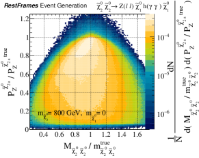
  1. 1.

    Apply the invisible mass JR VI.1, choosing MIsuperscriptsubscript𝑀IabsentM_{\footnotesize\mathrm{{\color[rgb]{0.12,0.3,0.17}\definecolor[named]{pgfstrokecolor}{rgb}{0.12,0.3,0.17}\textbf{I}}}}^{\footnotesize\leavevmode\nobreak\ } as the smallest possible quantity consistent with JR VI.4.1 and non-tachyonic neutralinos.

  2. 2.

    Apply the invisible rapidity JR V.1,
    choosing pI,zlabsuperscriptsubscript𝑝I𝑧labp_{\footnotesize\mathrm{{\color[rgb]{0.12,0.3,0.17}\definecolor[named]{pgfstrokecolor}{rgb}{0.12,0.3,0.17}\textbf{I}}},z}^{\footnotesize\leavevmode\nobreak\ \mathrm{\textbf{lab}}} using all the visible particles V.

  3. 3.

    Apply the contra-boost invariant JR VI.4.1,
    specifying the neutralino four vectors
    using the constraint Mχ~2a=Mχ~2bsuperscriptsubscript𝑀subscript~𝜒2𝑎absentsuperscriptsubscript𝑀subscript~𝜒2𝑏absentM_{\footnotesize\mathrm{{\color[rgb]{0.45,0.0,0.09}\definecolor[named]{pgfstrokecolor}{rgb}{0.45,0.0,0.09}\textbf{$\tilde{\chi}_{2a}$}}}}^{\footnotesize\leavevmode\nobreak\ }=M_{\footnotesize\mathrm{{\color[rgb]{0.45,0.0,0.09}\definecolor[named]{pgfstrokecolor}{rgb}{0.45,0.0,0.09}\textbf{$\tilde{\chi}_{2b}$}}}}^{\footnotesize\leavevmode\nobreak\ }.

Refer to caption
Figure 17: The distribution of the reconstructed Z𝑍Z boson momentum in the approximation of its production frame, as a function of the estimator Mcmsuperscriptsubscript𝑀cmabsentM_{\footnotesize\mathrm{{\color[rgb]{0.45,0.0,0.09}\definecolor[named]{pgfstrokecolor}{rgb}{0.45,0.0,0.09}\textbf{cm}}}}^{\footnotesize\leavevmode\nobreak\ }, for simulated χ~20χ~20Z(+)χ~10h(γγ)χ~10superscriptsubscript~𝜒20superscriptsubscript~𝜒20𝑍superscriptsuperscriptsuperscriptsubscript~𝜒10𝛾𝛾superscriptsubscript~𝜒10\tilde{\chi}_{2}^{0}\tilde{\chi}_{2}^{0}\rightarrow Z(\ell^{+}\ell^{-})\tilde{\chi}_{1}^{0}h(\gamma\gamma)\tilde{\chi}_{1}^{0} events. Each of the estimated quantities is normalized by the true value event-by-event.

Despite the complications involved with the non-trivial Z𝑍Z and Higgs masses, the contra-boost invariant jigsaw allows the kinematics of these visible systems in their production frames to be estimated with little bias. The reconstructed Z𝑍Z boson momentum in the approximation of its production frame, pZχ~2asuperscriptsubscript𝑝𝑍subscript~𝜒2𝑎p_{\footnotesize\mathrm{{\color[rgb]{0.1,0.1,0.44}\definecolor[named]{pgfstrokecolor}{rgb}{0.1,0.1,0.44}\textbf{$Z$}}}}^{\footnotesize\leavevmode\nobreak\ \mathrm{{\color[rgb]{0.45,0.0,0.09}\definecolor[named]{pgfstrokecolor}{rgb}{0.45,0.0,0.09}\textbf{$\tilde{\chi}_{2a}$}}}}, is shown in Fig. 17, where the similarities to Fig. 11 and 15 showing analogous observables from previous examples is striking. pZχ~2asuperscriptsubscript𝑝𝑍subscript~𝜒2𝑎p_{\footnotesize\mathrm{{\color[rgb]{0.1,0.1,0.44}\definecolor[named]{pgfstrokecolor}{rgb}{0.1,0.1,0.44}\textbf{$Z$}}}}^{\footnotesize\leavevmode\nobreak\ \mathrm{{\color[rgb]{0.45,0.0,0.09}\definecolor[named]{pgfstrokecolor}{rgb}{0.45,0.0,0.09}\textbf{$\tilde{\chi}_{2a}$}}}}, which is sensitive to the mass splitting between the two neutralino states, is estimated nearly independently of the total di-χ~20superscriptsubscript~𝜒20\tilde{\chi}_{2}^{0} mass, Mcmsuperscriptsubscript𝑀cmabsentM_{\footnotesize\mathrm{{\color[rgb]{0.45,0.0,0.09}\definecolor[named]{pgfstrokecolor}{rgb}{0.45,0.0,0.09}\textbf{cm}}}}^{\footnotesize\leavevmode\nobreak\ }, with a kinematic endpoint reliably falling at the true value. Relative to the previous examples, no additional distortion in the pZχ~2asuperscriptsubscript𝑝𝑍subscript~𝜒2𝑎p_{\footnotesize\mathrm{{\color[rgb]{0.1,0.1,0.44}\definecolor[named]{pgfstrokecolor}{rgb}{0.1,0.1,0.44}\textbf{$Z$}}}}^{\footnotesize\leavevmode\nobreak\ \mathrm{{\color[rgb]{0.45,0.0,0.09}\definecolor[named]{pgfstrokecolor}{rgb}{0.45,0.0,0.09}\textbf{$\tilde{\chi}_{2a}$}}}} distribution due to the Z𝑍Z and Higgs masses is visible.

Refer to caption
Figure 18: The distribution of the reconstructed Z𝑍Z decay angle, θZsubscript𝜃𝑍\theta_{\mathrm{{\color[rgb]{0.1,0.1,0.44}\definecolor[named]{pgfstrokecolor}{rgb}{0.1,0.1,0.44}\textbf{$Z$}}}}, as a function of the Higgs decay angle, θhsubscript𝜃\theta_{\mathrm{{\color[rgb]{0.1,0.1,0.44}\definecolor[named]{pgfstrokecolor}{rgb}{0.1,0.1,0.44}\textbf{$h$}}}}, for simulated χ~20χ~20Z(+)χ~10h(γγ)χ~10superscriptsubscript~𝜒20superscriptsubscript~𝜒20𝑍superscriptsuperscriptsuperscriptsubscript~𝜒10𝛾𝛾superscriptsubscript~𝜒10\tilde{\chi}_{2}^{0}\tilde{\chi}_{2}^{0}\rightarrow Z(\ell^{+}\ell^{-})\tilde{\chi}_{1}^{0}h(\gamma\gamma)\tilde{\chi}_{1}^{0} events. Both observables are shown relative to the true decay angles they are estimating, with angles in units radian.

That the approximations of the neutralino rest frames, χ~2asubscript~𝜒2𝑎\tilde{\chi}_{2a} and χ~2bsubscript~𝜒2𝑏\tilde{\chi}_{2b}, have a strong correspondence to the true ones can be seen by considering the reconstructed decay angles of the Z𝑍Z and Higgs bosons, which require knowledge of these reference frames as they are where the bosons are produced. The estimators θZsubscript𝜃𝑍\theta_{\mathrm{{\color[rgb]{0.1,0.1,0.44}\definecolor[named]{pgfstrokecolor}{rgb}{0.1,0.1,0.44}\textbf{$Z$}}}} and θhsubscript𝜃\theta_{\mathrm{{\color[rgb]{0.1,0.1,0.44}\definecolor[named]{pgfstrokecolor}{rgb}{0.1,0.1,0.44}\textbf{$h$}}}} can resolve the true quantities quite well, as demonstrated in Fig. 18, and are insensitive to the momentum of the center-of-mass system in the lab frame and the masses of the sparticles in the event. This is possible because the approximate χ~2asubscript~𝜒2𝑎\tilde{\chi}_{2a} and χ~2bsubscript~𝜒2𝑏\tilde{\chi}_{2b} rest frames have effectively inherited the invariance properties of the reference frames that proceed them in the decay tree, with longitudinal and contra-boost invariant definitions. As was the case for the hγγ𝛾𝛾h\rightarrow\gamma\gamma decays in Section V.3, the approximate reconstruction of the intermediate decay frames in the event allows the decay angles of these visible systems to be estimated with excellent precision.

VII More Jigsaws for Two Invisible Particles

In this section, we expand the library of JR’s designed to study final states with two invisible particles by considering a series of examples motivated by top pair production. In fully-leptonic tt¯𝑡¯𝑡t\bar{t} events, two top quarks each decay to a b𝑏b-quark and a leptonically decaying W𝑊W boson, resulting in a final state with four visible, reconstructable particles, and two neutrinos. The additional two visible particles relative to the examples of Section VI provide both new challenges and opportunities. While a combinatoric ambiguity must be resolved as to which b𝑏b-tagged jet to associate with each lepton, more visible particles allow for better resolution of the under-constrained neutrino kinematics.

We consider three examples with this same final state, including non-resonant top pair-production (Section VII.1), resonant tt¯𝑡¯𝑡t\bar{t} production through a heavy Higgs boson (Section VII.2), and stop quark pair-production with decays through charginos and sneutrinos (Section VII.3). Additional JR’s for studying this final state are described in Section VII.1 with several approaches compared throughout the examples.

VII.1 tt¯bW(ν)bW(ν)𝑡¯𝑡𝑏𝑊𝜈𝑏𝑊𝜈t\bar{t}\rightarrow bW(\ell\nu)bW(\ell\nu) at a hadron collider

The first case we consider with four visible and two invisible particles in the final state is top pair production at a hadron collider, with subsequent decays to b𝑏b-quarks, leptons, and neutrinos via intermediate W𝑊W bosons. We assume in these events that two b𝑏b-tagged jets are identified and reconstructed in the detector, with measured four vectors 𝐩balabsuperscriptsubscript𝐩subscript𝑏𝑎lab\mathbf{p}_{\footnotesize\mathrm{{\color[rgb]{0.1,0.1,0.44}\definecolor[named]{pgfstrokecolor}{rgb}{0.1,0.1,0.44}\textbf{$b_{a}$}}}}^{\footnotesize\leavevmode\nobreak\ \mathrm{\textbf{lab}}} and 𝐩bblabsuperscriptsubscript𝐩subscript𝑏𝑏lab\mathbf{p}_{\footnotesize\mathrm{{\color[rgb]{0.1,0.1,0.44}\definecolor[named]{pgfstrokecolor}{rgb}{0.1,0.1,0.44}\textbf{$b_{b}$}}}}^{\footnotesize\leavevmode\nobreak\ \mathrm{\textbf{lab}}}, along with two leptons, with four vectors 𝐩alabsuperscriptsubscript𝐩subscript𝑎lab\mathbf{p}_{\footnotesize\mathrm{{\color[rgb]{0.1,0.1,0.44}\definecolor[named]{pgfstrokecolor}{rgb}{0.1,0.1,0.44}\textbf{$\ell_{a}$}}}}^{\footnotesize\leavevmode\nobreak\ \mathrm{\textbf{lab}}} and 𝐩blabsuperscriptsubscript𝐩subscript𝑏lab\mathbf{p}_{\footnotesize\mathrm{{\color[rgb]{0.1,0.1,0.44}\definecolor[named]{pgfstrokecolor}{rgb}{0.1,0.1,0.44}\textbf{$\ell_{b}$}}}}^{\footnotesize\leavevmode\nobreak\ \mathrm{\textbf{lab}}}. The measured ETmisssuperscriptsubscript𝐸𝑇miss\vec{E}_{T}^{\rm miss}  is interpreted as the transverse momentum of the di-neutrino system, pI,Tlabsuperscriptsubscript𝑝I𝑇lab\vec{p}_{\footnotesize\mathrm{{\color[rgb]{0.12,0.3,0.17}\definecolor[named]{pgfstrokecolor}{rgb}{0.12,0.3,0.17}\textbf{I}}},T}^{\footnotesize\leavevmode\nobreak\ \mathrm{\textbf{lab}}}, with I={νa,νb}Isubscript𝜈𝑎subscript𝜈𝑏\mathrm{{\color[rgb]{0.12,0.3,0.17}\definecolor[named]{pgfstrokecolor}{rgb}{0.12,0.3,0.17}\textbf{I}}}=\{\mathrm{{\color[rgb]{0.12,0.3,0.17}\definecolor[named]{pgfstrokecolor}{rgb}{0.12,0.3,0.17}\textbf{$\nu_{a}$}}},\mathrm{{\color[rgb]{0.12,0.3,0.17}\definecolor[named]{pgfstrokecolor}{rgb}{0.12,0.3,0.17}\textbf{$\nu_{b}$}}}\}. The decay tree used for analyzing this final state is shown in Fig. 19.
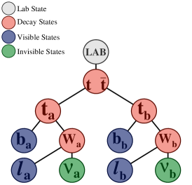
Refer to caption
Figure 19: The decay tree for analyzing tt¯bW(ν)bW(ν)𝑡¯𝑡𝑏𝑊𝜈𝑏𝑊𝜈t\bar{t}\rightarrow bW(\ell\nu)bW(\ell\nu) events. Four visible particles are reconstructed in the final state, along with two invisible particles which are constrained by the measured ETmisssuperscriptsubscript𝐸𝑇miss\vec{E}_{T}^{\rm miss}. There are several masses of interest in the event, with two intermediate top quarks and two W𝑊W bosons appearing in the decays.

In addition to unknowns associated with invisible particles in the event, there is a combinatoric ambiguity in deciding which reconstructed b𝑏b-tagged jet should be associated with each lepton. We assume that we are unable to reliably distinguish between b𝑏b-tagged jets initiated by b𝑏b-quarks and those from anti-particles, so we make this choice solely relying on the kinematics of each event. Defining Va={ba,a}Vasubscript𝑏𝑎subscript𝑎\mathrm{{\color[rgb]{0.1,0.1,0.44}\definecolor[named]{pgfstrokecolor}{rgb}{0.1,0.1,0.44}\textbf{V${}_{a}$}}}=\{\mathrm{{\color[rgb]{0.1,0.1,0.44}\definecolor[named]{pgfstrokecolor}{rgb}{0.1,0.1,0.44}\textbf{$b_{a}$}}},\mathrm{{\color[rgb]{0.1,0.1,0.44}\definecolor[named]{pgfstrokecolor}{rgb}{0.1,0.1,0.44}\textbf{$\ell_{a}$}}}\} and Vb={bb,b}Vbsubscript𝑏𝑏subscript𝑏\mathrm{{\color[rgb]{0.1,0.1,0.44}\definecolor[named]{pgfstrokecolor}{rgb}{0.1,0.1,0.44}\textbf{V${}_{b}$}}}=\{\mathrm{{\color[rgb]{0.1,0.1,0.44}\definecolor[named]{pgfstrokecolor}{rgb}{0.1,0.1,0.44}\textbf{$b_{b}$}}},\mathrm{{\color[rgb]{0.1,0.1,0.44}\definecolor[named]{pgfstrokecolor}{rgb}{0.1,0.1,0.44}\textbf{$\ell_{b}$}}}\} as the two sets of visible particles associated with each top decay, we define a JR to choose the b/𝑏\mathrm{{\color[rgb]{0.1,0.1,0.44}\definecolor[named]{pgfstrokecolor}{rgb}{0.1,0.1,0.44}\textbf{$b$}}}/\mathrm{{\color[rgb]{0.1,0.1,0.44}\definecolor[named]{pgfstrokecolor}{rgb}{0.1,0.1,0.44}\textbf{$\ell$}}} pairing which minimizes the function MVa 2+MVb 2superscriptsubscript𝑀Va2superscriptsubscript𝑀Vb2M_{\footnotesize\mathrm{{\color[rgb]{0.1,0.1,0.44}\definecolor[named]{pgfstrokecolor}{rgb}{0.1,0.1,0.44}\textbf{V${}_{a}$}}}}^{\footnotesize\leavevmode\nobreak\ 2}+M_{\footnotesize\mathrm{{\color[rgb]{0.1,0.1,0.44}\definecolor[named]{pgfstrokecolor}{rgb}{0.1,0.1,0.44}\textbf{V${}_{b}$}}}}^{\footnotesize\leavevmode\nobreak\ 2}. This is a simple, and generally correct, prescription as it chooses combinations where the sum of four vector inner products is smallest, effectively pairing particles flying closest together as expected from a common decay source. More generally, we can define this combinatoric JR as follows:

Jigsaw Rule VII.1 (Combinatoric Minimization)

If there is a set of n𝑛n visible particles, V={V1,,Vn}VV1Vn\mathrm{{\color[rgb]{0.1,0.1,0.44}\definecolor[named]{pgfstrokecolor}{rgb}{0.1,0.1,0.44}\textbf{V}}}=\{\mathrm{{\color[rgb]{0.1,0.1,0.44}\definecolor[named]{pgfstrokecolor}{rgb}{0.1,0.1,0.44}\textbf{V${}_{1}$}}},\cdots,\mathrm{{\color[rgb]{0.1,0.1,0.44}\definecolor[named]{pgfstrokecolor}{rgb}{0.1,0.1,0.44}\textbf{V${}_{n}$}}}\}, we can choose a partition of V into mn𝑚𝑛m\leq n subsets, PV={SV1,,SVm}subscript𝑃Vsubscript𝑆V1subscript𝑆VmP_{\mathrm{{\color[rgb]{0.1,0.1,0.44}\definecolor[named]{pgfstrokecolor}{rgb}{0.1,0.1,0.44}\textbf{V}}}}=\{S_{\mathrm{{\color[rgb]{0.1,0.1,0.44}\definecolor[named]{pgfstrokecolor}{rgb}{0.1,0.1,0.44}\textbf{V$1$}}}},\cdots,S_{\mathrm{{\color[rgb]{0.1,0.1,0.44}\definecolor[named]{pgfstrokecolor}{rgb}{0.1,0.1,0.44}\textbf{V$m$}}}}\}, by minimizing a chosen metric over the space of all valid partitions, PVVsubscript𝑃VsubscriptVP_{\mathrm{{\color[rgb]{0.1,0.1,0.44}\definecolor[named]{pgfstrokecolor}{rgb}{0.1,0.1,0.44}\textbf{V}}}}\in\mathbb{P}_{\mathrm{{\color[rgb]{0.1,0.1,0.44}\definecolor[named]{pgfstrokecolor}{rgb}{0.1,0.1,0.44}\textbf{V}}}}.

A partition, PVsubscript𝑃VP_{\mathrm{{\color[rgb]{0.1,0.1,0.44}\definecolor[named]{pgfstrokecolor}{rgb}{0.1,0.1,0.44}\textbf{V}}}}, is valid if it satisfies the conditions

(a)𝑎\displaystyle(a) SVPVSV=Vsubscriptsubscript𝑆Vsubscript𝑃Vsubscript𝑆VV\displaystyle\leavevmode\nobreak\ \bigcup_{S_{\mathrm{{\color[rgb]{0.1,0.1,0.44}\definecolor[named]{pgfstrokecolor}{rgb}{0.1,0.1,0.44}\textbf{V}}}}\in P_{\mathrm{{\color[rgb]{0.1,0.1,0.44}\definecolor[named]{pgfstrokecolor}{rgb}{0.1,0.1,0.44}\textbf{V}}}}}S_{\mathrm{{\color[rgb]{0.1,0.1,0.44}\definecolor[named]{pgfstrokecolor}{rgb}{0.1,0.1,0.44}\textbf{V}}}}=\mathrm{{\color[rgb]{0.1,0.1,0.44}\definecolor[named]{pgfstrokecolor}{rgb}{0.1,0.1,0.44}\textbf{V}}}
(b)𝑏\displaystyle(b) SVa,SVbPV,for-allsubscript𝑆Vasubscript𝑆Vbsubscript𝑃V\displaystyle\leavevmode\nobreak\ \forall S_{\mathrm{{\color[rgb]{0.1,0.1,0.44}\definecolor[named]{pgfstrokecolor}{rgb}{0.1,0.1,0.44}\textbf{V$a$}}}},S_{\mathrm{{\color[rgb]{0.1,0.1,0.44}\definecolor[named]{pgfstrokecolor}{rgb}{0.1,0.1,0.44}\textbf{V$b$}}}}\in P_{\mathrm{{\color[rgb]{0.1,0.1,0.44}\definecolor[named]{pgfstrokecolor}{rgb}{0.1,0.1,0.44}\textbf{V}}}}\leavevmode\nobreak\ ,
SVaSVbSVaSVb=subscript𝑆Vasubscript𝑆Vbsubscript𝑆Vasubscript𝑆Vb\displaystyle\leavevmode\nobreak\ S_{\mathrm{{\color[rgb]{0.1,0.1,0.44}\definecolor[named]{pgfstrokecolor}{rgb}{0.1,0.1,0.44}\textbf{V$a$}}}}\neq S_{\mathrm{{\color[rgb]{0.1,0.1,0.44}\definecolor[named]{pgfstrokecolor}{rgb}{0.1,0.1,0.44}\textbf{V$b$}}}}\implies S_{\mathrm{{\color[rgb]{0.1,0.1,0.44}\definecolor[named]{pgfstrokecolor}{rgb}{0.1,0.1,0.44}\textbf{V$a$}}}}\cap S_{\mathrm{{\color[rgb]{0.1,0.1,0.44}\definecolor[named]{pgfstrokecolor}{rgb}{0.1,0.1,0.44}\textbf{V$b$}}}}=\emptyset
(c)𝑐\displaystyle(c) |SVi|or=ni1foranyrequirementsni,subscript𝑆Vi𝑜𝑟subscript𝑛𝑖1𝑓𝑜𝑟𝑎𝑛𝑦𝑟𝑒𝑞𝑢𝑖𝑟𝑒𝑚𝑒𝑛𝑡𝑠subscript𝑛𝑖\displaystyle\leavevmode\nobreak\ |S_{\mathrm{{\color[rgb]{0.1,0.1,0.44}\definecolor[named]{pgfstrokecolor}{rgb}{0.1,0.1,0.44}\textbf{V$i$}}}}|\geq or=n_{i}\geq 1\leavevmode\nobreak\ for\leavevmode\nobreak\ any\leavevmode\nobreak\ requirements\leavevmode\nobreak\ n_{i},
(d)𝑑\displaystyle(d) Q(SVi)=qiforanychargerequirementsqi.𝑄subscript𝑆Visubscript𝑞𝑖𝑓𝑜𝑟𝑎𝑛𝑦𝑐𝑎𝑟𝑔𝑒𝑟𝑒𝑞𝑢𝑖𝑟𝑒𝑚𝑒𝑛𝑡𝑠subscript𝑞𝑖\displaystyle\leavevmode\nobreak\ Q(S_{\mathrm{{\color[rgb]{0.1,0.1,0.44}\definecolor[named]{pgfstrokecolor}{rgb}{0.1,0.1,0.44}\textbf{V$i$}}}})=q_{i}\leavevmode\nobreak\ for\leavevmode\nobreak\ any\leavevmode\nobreak\ charge\leavevmode\nobreak\ requirements\leavevmode\nobreak\ q_{i}\leavevmode\nobreak\ .

We assume there is at least one valid partition in each event, |V|1containsabsentsubscriptV1\ni|\mathbb{P}_{\mathrm{{\color[rgb]{0.1,0.1,0.44}\definecolor[named]{pgfstrokecolor}{rgb}{0.1,0.1,0.44}\textbf{V}}}}|\geq 1, and choose a partition, P^Vsubscript^𝑃V\hat{P}_{\mathrm{{\color[rgb]{0.1,0.1,0.44}\definecolor[named]{pgfstrokecolor}{rgb}{0.1,0.1,0.44}\textbf{V}}}}, from this set by minimizing a function of the event’s kinematics, f(PV)𝑓subscript𝑃Vf(P_{\mathrm{{\color[rgb]{0.1,0.1,0.44}\definecolor[named]{pgfstrokecolor}{rgb}{0.1,0.1,0.44}\textbf{V}}}}), that is sensitive to this choice, with

f(P^V)=minPVVf(PV).𝑓subscript^𝑃Vsubscriptsubscript𝑃VsubscriptV𝑓subscript𝑃V\displaystyle f(\hat{P}_{\mathrm{{\color[rgb]{0.1,0.1,0.44}\definecolor[named]{pgfstrokecolor}{rgb}{0.1,0.1,0.44}\textbf{V}}}})=\min_{P_{\mathrm{{\color[rgb]{0.1,0.1,0.44}\definecolor[named]{pgfstrokecolor}{rgb}{0.1,0.1,0.44}\textbf{V}}}}\in\mathbb{P}_{\mathrm{{\color[rgb]{0.1,0.1,0.44}\definecolor[named]{pgfstrokecolor}{rgb}{0.1,0.1,0.44}\textbf{V}}}}}f(P_{\mathrm{{\color[rgb]{0.1,0.1,0.44}\definecolor[named]{pgfstrokecolor}{rgb}{0.1,0.1,0.44}\textbf{V}}}})\leavevmode\nobreak\ . (47)

If the function f(PV)𝑓subscript𝑃Vf(P_{\mathrm{{\color[rgb]{0.1,0.1,0.44}\definecolor[named]{pgfstrokecolor}{rgb}{0.1,0.1,0.44}\textbf{V}}}}) depends on other unknown kinematic or combinatoric information that depends on the application of other JR’s which, in-turn, depend on the choice P^Vsubscript^𝑃V\hat{P}_{\mathrm{{\color[rgb]{0.1,0.1,0.44}\definecolor[named]{pgfstrokecolor}{rgb}{0.1,0.1,0.44}\textbf{V}}}}, then these JR’s are evaluated independently for each value PVsubscript𝑃VP_{\mathrm{{\color[rgb]{0.1,0.1,0.44}\definecolor[named]{pgfstrokecolor}{rgb}{0.1,0.1,0.44}\textbf{V}}}} in Eq. 47.

JR case VII.1.1 (Minimize Masses Squared)

A convenient choice for f(PV)𝑓subscript𝑃Vf(P_{\mathrm{{\color[rgb]{0.1,0.1,0.44}\definecolor[named]{pgfstrokecolor}{rgb}{0.1,0.1,0.44}\textbf{V}}}}) is the sum of four vector inner products of the elements of the m𝑚m sets in a partition, potentially including other particles in the event. With O={O1,,Om}OO1Om\mathrm{{\color[rgb]{0.1,0.1,0.44}\definecolor[named]{pgfstrokecolor}{rgb}{0.1,0.1,0.44}\textbf{O}}}=\{\mathrm{{\color[rgb]{0.1,0.1,0.44}\definecolor[named]{pgfstrokecolor}{rgb}{0.1,0.1,0.44}\textbf{O${}_{1}$}}},\cdots,\mathrm{{\color[rgb]{0.1,0.1,0.44}\definecolor[named]{pgfstrokecolor}{rgb}{0.1,0.1,0.44}\textbf{O${}_{m}$}}}\} the set of other particles associated with each combinatoric subset in a partition PVsubscript𝑃VP_{\mathrm{{\color[rgb]{0.1,0.1,0.44}\definecolor[named]{pgfstrokecolor}{rgb}{0.1,0.1,0.44}\textbf{V}}}}, we can define f(PV)𝑓subscript𝑃Vf(P_{\mathrm{{\color[rgb]{0.1,0.1,0.44}\definecolor[named]{pgfstrokecolor}{rgb}{0.1,0.1,0.44}\textbf{V}}}}) as

f(PV)𝑓subscript𝑃V\displaystyle f(P_{\mathrm{{\color[rgb]{0.1,0.1,0.44}\definecolor[named]{pgfstrokecolor}{rgb}{0.1,0.1,0.44}\textbf{V}}}}) =\displaystyle= i=1mMSViOi 2=i=1m(𝐩SVi+𝐩Oi)2.superscriptsubscript𝑖1𝑚superscriptsubscript𝑀subscript𝑆ViOi2superscriptsubscript𝑖1𝑚superscriptsuperscriptsubscript𝐩subscript𝑆Viabsentsuperscriptsubscript𝐩Oiabsent2\displaystyle\sum_{i=1}^{m}M_{\footnotesize S_{\mathrm{{\color[rgb]{0.1,0.1,0.44}\definecolor[named]{pgfstrokecolor}{rgb}{0.1,0.1,0.44}\textbf{V$i$}}}}\mathrm{{\color[rgb]{0.1,0.1,0.44}\definecolor[named]{pgfstrokecolor}{rgb}{0.1,0.1,0.44}\textbf{O${}_{i}$}}}}^{\footnotesize\leavevmode\nobreak\ 2}=\sum_{i=1}^{m}(\mathbf{p}_{\footnotesize S_{\mathrm{{\color[rgb]{0.1,0.1,0.44}\definecolor[named]{pgfstrokecolor}{rgb}{0.1,0.1,0.44}\textbf{V$i$}}}}}^{\footnotesize\leavevmode\nobreak\ }+\mathbf{p}_{\footnotesize\mathrm{{\color[rgb]{0.1,0.1,0.44}\definecolor[named]{pgfstrokecolor}{rgb}{0.1,0.1,0.44}\textbf{O${}_{i}$}}}}^{\footnotesize\leavevmode\nobreak\ })^{2}\leavevmode\nobreak\ . (48)

The appeal of this functional form is that it can be linearly factorized, in the sense that if PV={SV1,,SVm}superscriptsubscript𝑃Vsuperscriptsubscript𝑆V1superscriptsubscript𝑆superscriptVmP_{\mathrm{{\color[rgb]{0.1,0.1,0.44}\definecolor[named]{pgfstrokecolor}{rgb}{0.1,0.1,0.44}\textbf{V}}}}^{{}^{\prime}}=\{S_{\mathrm{{\color[rgb]{0.1,0.1,0.44}\definecolor[named]{pgfstrokecolor}{rgb}{0.1,0.1,0.44}\textbf{V$1$}}}}^{{}^{\prime}},\cdots,S_{\mathrm{{\color[rgb]{0.1,0.1,0.44}\definecolor[named]{pgfstrokecolor}{rgb}{0.1,0.1,0.44}\textbf{V$m$}}}^{{}^{\prime}}}^{{}^{\prime}}\} is a partition of V where PVsubscript𝑃VP_{\mathrm{{\color[rgb]{0.1,0.1,0.44}\definecolor[named]{pgfstrokecolor}{rgb}{0.1,0.1,0.44}\textbf{V}}}} is its refinement, such that |PV||PV|subscript𝑃Vsuperscriptsubscript𝑃V|P_{\mathrm{{\color[rgb]{0.1,0.1,0.44}\definecolor[named]{pgfstrokecolor}{rgb}{0.1,0.1,0.44}\textbf{V}}}}|\leq|P_{\mathrm{{\color[rgb]{0.1,0.1,0.44}\definecolor[named]{pgfstrokecolor}{rgb}{0.1,0.1,0.44}\textbf{V}}}}^{{}^{\prime}}| and SVPV,SVPVwithSVSVformulae-sequencefor-allsubscript𝑆Vsubscript𝑃Vsuperscriptsubscript𝑆Vsuperscriptsubscript𝑃V𝑤𝑖𝑡subscript𝑆Vsuperscriptsubscript𝑆V\forall S_{\mathrm{{\color[rgb]{0.1,0.1,0.44}\definecolor[named]{pgfstrokecolor}{rgb}{0.1,0.1,0.44}\textbf{V}}}}\in P_{\mathrm{{\color[rgb]{0.1,0.1,0.44}\definecolor[named]{pgfstrokecolor}{rgb}{0.1,0.1,0.44}\textbf{V}}}},\leavevmode\nobreak\ \exists\leavevmode\nobreak\ S_{\mathrm{{\color[rgb]{0.1,0.1,0.44}\definecolor[named]{pgfstrokecolor}{rgb}{0.1,0.1,0.44}\textbf{V}}}}^{{}^{\prime}}\in P_{\mathrm{{\color[rgb]{0.1,0.1,0.44}\definecolor[named]{pgfstrokecolor}{rgb}{0.1,0.1,0.44}\textbf{V}}}}^{{}^{\prime}}\leavevmode\nobreak\ with\leavevmode\nobreak\ S_{\mathrm{{\color[rgb]{0.1,0.1,0.44}\definecolor[named]{pgfstrokecolor}{rgb}{0.1,0.1,0.44}\textbf{V}}}}\subseteq S_{\mathrm{{\color[rgb]{0.1,0.1,0.44}\definecolor[named]{pgfstrokecolor}{rgb}{0.1,0.1,0.44}\textbf{V}}}}^{{}^{\prime}}, then f(PV)𝑓subscript𝑃Vf(P_{\mathrm{{\color[rgb]{0.1,0.1,0.44}\definecolor[named]{pgfstrokecolor}{rgb}{0.1,0.1,0.44}\textbf{V}}}}) can be expressed as

f(PV)=SVPVf(SV)=SVPVSVSVf(SV).𝑓subscript𝑃Vsubscriptsuperscriptsubscript𝑆Vsuperscriptsubscript𝑃V𝑓superscriptsubscript𝑆Vsubscriptsuperscriptsubscript𝑆Vsuperscriptsubscript𝑃Vsubscriptsubscript𝑆Vsuperscriptsubscript𝑆V𝑓subscript𝑆V\displaystyle f(P_{\mathrm{{\color[rgb]{0.1,0.1,0.44}\definecolor[named]{pgfstrokecolor}{rgb}{0.1,0.1,0.44}\textbf{V}}}})=\sum_{S_{\mathrm{{\color[rgb]{0.1,0.1,0.44}\definecolor[named]{pgfstrokecolor}{rgb}{0.1,0.1,0.44}\textbf{V}}}}^{{}^{\prime}}\in P_{\mathrm{{\color[rgb]{0.1,0.1,0.44}\definecolor[named]{pgfstrokecolor}{rgb}{0.1,0.1,0.44}\textbf{V}}}}^{{}^{\prime}}}f(S_{\mathrm{{\color[rgb]{0.1,0.1,0.44}\definecolor[named]{pgfstrokecolor}{rgb}{0.1,0.1,0.44}\textbf{V}}}}^{{}^{\prime}})=\sum_{S_{\mathrm{{\color[rgb]{0.1,0.1,0.44}\definecolor[named]{pgfstrokecolor}{rgb}{0.1,0.1,0.44}\textbf{V}}}}^{{}^{\prime}}\in P_{\mathrm{{\color[rgb]{0.1,0.1,0.44}\definecolor[named]{pgfstrokecolor}{rgb}{0.1,0.1,0.44}\textbf{V}}}}^{{}^{\prime}}}\sum_{S_{\mathrm{{\color[rgb]{0.1,0.1,0.44}\definecolor[named]{pgfstrokecolor}{rgb}{0.1,0.1,0.44}\textbf{V}}}}\in S_{\mathrm{{\color[rgb]{0.1,0.1,0.44}\definecolor[named]{pgfstrokecolor}{rgb}{0.1,0.1,0.44}\textbf{V}}}}^{{}^{\prime}}}f(S_{\mathrm{{\color[rgb]{0.1,0.1,0.44}\definecolor[named]{pgfstrokecolor}{rgb}{0.1,0.1,0.44}\textbf{V}}}})\leavevmode\nobreak\ . (49)

This implies one can use recursive applications of this JR corresponding to a sequence of progressively fine partitions of V, effectively minimizing the same function as a single application, but in factorized steps, potentially improving the resolution of intermediate particle structure in an event if chosen correspondingly.

With this choice for the b/𝑏\mathrm{{\color[rgb]{0.1,0.1,0.44}\definecolor[named]{pgfstrokecolor}{rgb}{0.1,0.1,0.44}\textbf{$b$}}}/\mathrm{{\color[rgb]{0.1,0.1,0.44}\definecolor[named]{pgfstrokecolor}{rgb}{0.1,0.1,0.44}\textbf{$\ell$}}} pairing in each event, the remaining unknowns associated with the neutrinos are the same as in each of the examples of Section VI, and can be represented as the mass of the total invisible system, MIsuperscriptsubscript𝑀IabsentM_{\footnotesize\mathrm{{\color[rgb]{0.12,0.3,0.17}\definecolor[named]{pgfstrokecolor}{rgb}{0.12,0.3,0.17}\textbf{I}}}}^{\footnotesize\leavevmode\nobreak\ }, its momentum along the beam axis, the orientation of the “decay” of I into two neutrinos, and the two individual neutrino masses. The increased number of visible particles means that there are choices in strategy when applying the contra-boost invariant JR VI.4 to resolve these unknowns. For example, the two leptons could be paired with the two neutrinos, and a contra-boost invariant JR imposing MWa=MWbsuperscriptsubscript𝑀subscript𝑊𝑎absentsuperscriptsubscript𝑀subscript𝑊𝑏absentM_{\footnotesize\mathrm{{\color[rgb]{0.45,0.0,0.09}\definecolor[named]{pgfstrokecolor}{rgb}{0.45,0.0,0.09}\textbf{$W_{a}$}}}}^{\footnotesize\leavevmode\nobreak\ }=M_{\footnotesize\mathrm{{\color[rgb]{0.45,0.0,0.09}\definecolor[named]{pgfstrokecolor}{rgb}{0.45,0.0,0.09}\textbf{$W_{b}$}}}}^{\footnotesize\leavevmode\nobreak\ } applied. Alternatively, the two b/𝑏\mathrm{{\color[rgb]{0.1,0.1,0.44}\definecolor[named]{pgfstrokecolor}{rgb}{0.1,0.1,0.44}\textbf{$b$}}}/\mathrm{{\color[rgb]{0.1,0.1,0.44}\definecolor[named]{pgfstrokecolor}{rgb}{0.1,0.1,0.44}\textbf{$\ell$}}} pairs, Va and Vb, can be used, imposing the constraint Mta=Mtbsuperscriptsubscript𝑀subscript𝑡𝑎absentsuperscriptsubscript𝑀subscript𝑡𝑏absentM_{\footnotesize\mathrm{{\color[rgb]{0.45,0.0,0.09}\definecolor[named]{pgfstrokecolor}{rgb}{0.45,0.0,0.09}\textbf{$t_{a}$}}}}^{\footnotesize\leavevmode\nobreak\ }=M_{\footnotesize\mathrm{{\color[rgb]{0.45,0.0,0.09}\definecolor[named]{pgfstrokecolor}{rgb}{0.45,0.0,0.09}\textbf{$t_{b}$}}}}^{\footnotesize\leavevmode\nobreak\ }. While both approaches are perfectly applicable to this final state, there are cases where these mass equality constraints may not be appropriate. Furthermore, there may be cases where insisting on contra-boost invariance at the cost of the estimators of invisible particle masses acquiring additional mass (as described thoroughly in Section VI) may not be desirable. To address these cases, we introduce additional JR’s for choosing the degrees of freedom associated with splitting apart a di-invisible system.

We take the same approach as Section VI, imagining that we are able to evaluate each of the visible four vectors in the event in the total center-of-mass frame, cm=tt¯={V,I}cm𝑡¯𝑡VI\mathrm{{\color[rgb]{0.45,0.0,0.09}\definecolor[named]{pgfstrokecolor}{rgb}{0.45,0.0,0.09}\textbf{cm}}}=\mathrm{{\color[rgb]{0.45,0.0,0.09}\definecolor[named]{pgfstrokecolor}{rgb}{0.45,0.0,0.09}\textbf{$t\bar{t}$}}}=\{\mathrm{{\color[rgb]{0.1,0.1,0.44}\definecolor[named]{pgfstrokecolor}{rgb}{0.1,0.1,0.44}\textbf{V}}},\mathrm{{\color[rgb]{0.12,0.3,0.17}\definecolor[named]{pgfstrokecolor}{rgb}{0.12,0.3,0.17}\textbf{I}}}\}, and the four vector associated with the total invisible system, 𝐩Icmsuperscriptsubscript𝐩Icm\mathbf{p}_{\footnotesize\mathrm{{\color[rgb]{0.12,0.3,0.17}\definecolor[named]{pgfstrokecolor}{rgb}{0.12,0.3,0.17}\textbf{I}}}}^{\footnotesize\leavevmode\nobreak\ \mathrm{{\color[rgb]{0.45,0.0,0.09}\definecolor[named]{pgfstrokecolor}{rgb}{0.45,0.0,0.09}\textbf{cm}}}}. Additionally, we now impose exact constraints on the individual neutrino masses, with Mνa=Mνb=0superscriptsubscript𝑀subscript𝜈𝑎absentsuperscriptsubscript𝑀subscript𝜈𝑏absent0M_{\footnotesize\mathrm{{\color[rgb]{0.12,0.3,0.17}\definecolor[named]{pgfstrokecolor}{rgb}{0.12,0.3,0.17}\textbf{$\nu_{a}$}}}}^{\footnotesize\leavevmode\nobreak\ }=M_{\footnotesize\mathrm{{\color[rgb]{0.12,0.3,0.17}\definecolor[named]{pgfstrokecolor}{rgb}{0.12,0.3,0.17}\textbf{$\nu_{b}$}}}}^{\footnotesize\leavevmode\nobreak\ }=0. The remaining unknowns are associated with how the momentum of these two individual neutrinos are chosen in this reference frame, subject to the constraints

pνacm+pνbcm+pVcm=0superscriptsubscript𝑝subscript𝜈𝑎cmsuperscriptsubscript𝑝subscript𝜈𝑏cmsuperscriptsubscript𝑝Vcm0\displaystyle\vec{p}_{\footnotesize\mathrm{{\color[rgb]{0.12,0.3,0.17}\definecolor[named]{pgfstrokecolor}{rgb}{0.12,0.3,0.17}\textbf{$\nu_{a}$}}}}^{\footnotesize\leavevmode\nobreak\ \mathrm{{\color[rgb]{0.45,0.0,0.09}\definecolor[named]{pgfstrokecolor}{rgb}{0.45,0.0,0.09}\textbf{cm}}}}+\vec{p}_{\footnotesize\mathrm{{\color[rgb]{0.12,0.3,0.17}\definecolor[named]{pgfstrokecolor}{rgb}{0.12,0.3,0.17}\textbf{$\nu_{b}$}}}}^{\footnotesize\leavevmode\nobreak\ \mathrm{{\color[rgb]{0.45,0.0,0.09}\definecolor[named]{pgfstrokecolor}{rgb}{0.45,0.0,0.09}\textbf{cm}}}}+\vec{p}_{\footnotesize\mathrm{{\color[rgb]{0.1,0.1,0.44}\definecolor[named]{pgfstrokecolor}{rgb}{0.1,0.1,0.44}\textbf{V}}}}^{\footnotesize\leavevmode\nobreak\ \mathrm{{\color[rgb]{0.45,0.0,0.09}\definecolor[named]{pgfstrokecolor}{rgb}{0.45,0.0,0.09}\textbf{cm}}}}=0 (50)
(𝐩νacm+𝐩νbcm)2=MI 2,superscriptsuperscriptsubscript𝐩subscript𝜈𝑎cmsuperscriptsubscript𝐩subscript𝜈𝑏cm2superscriptsubscript𝑀I2\displaystyle(\mathbf{p}_{\footnotesize\mathrm{{\color[rgb]{0.12,0.3,0.17}\definecolor[named]{pgfstrokecolor}{rgb}{0.12,0.3,0.17}\textbf{$\nu_{a}$}}}}^{\footnotesize\leavevmode\nobreak\ \mathrm{{\color[rgb]{0.45,0.0,0.09}\definecolor[named]{pgfstrokecolor}{rgb}{0.45,0.0,0.09}\textbf{cm}}}}+\mathbf{p}_{\footnotesize\mathrm{{\color[rgb]{0.12,0.3,0.17}\definecolor[named]{pgfstrokecolor}{rgb}{0.12,0.3,0.17}\textbf{$\nu_{b}$}}}}^{\footnotesize\leavevmode\nobreak\ \mathrm{{\color[rgb]{0.45,0.0,0.09}\definecolor[named]{pgfstrokecolor}{rgb}{0.45,0.0,0.09}\textbf{cm}}}})^{2}=M_{\footnotesize\mathrm{{\color[rgb]{0.12,0.3,0.17}\definecolor[named]{pgfstrokecolor}{rgb}{0.12,0.3,0.17}\textbf{I}}}}^{\footnotesize\leavevmode\nobreak\ 2}\leavevmode\nobreak\ ,

corresponding to two under-constrained degrees of freedom.

As the individual neutrino masses are fixed, and the masses mVasuperscriptsubscript𝑚Vaabsentm_{\footnotesize\mathrm{{\color[rgb]{0.1,0.1,0.44}\definecolor[named]{pgfstrokecolor}{rgb}{0.1,0.1,0.44}\textbf{V${}_{a}$}}}}^{\footnotesize\leavevmode\nobreak\ } and mVbsuperscriptsubscript𝑚Vbabsentm_{\footnotesize\mathrm{{\color[rgb]{0.1,0.1,0.44}\definecolor[named]{pgfstrokecolor}{rgb}{0.1,0.1,0.44}\textbf{V${}_{b}$}}}}^{\footnotesize\leavevmode\nobreak\ } will assume unequal, non-trivial values in these events, we are unable set our approximations of the two top masses exactly equal, as such a constraint could lead to tachyonic approximations of the neutrino four vectors. If we want to effectively minimize these masses w.r.t. our choices for the neutrino momentum, we must choose a new mass-sensitive metric.

A suitable choice for this metric can be seen more clearly if we instead work in the rest frame of the di-neutrino system, I. With our assumed knowledge of 𝐩Icmsuperscriptsubscript𝐩Icm\mathbf{p}_{\footnotesize\mathrm{{\color[rgb]{0.12,0.3,0.17}\definecolor[named]{pgfstrokecolor}{rgb}{0.12,0.3,0.17}\textbf{I}}}}^{\footnotesize\leavevmode\nobreak\ \mathrm{{\color[rgb]{0.45,0.0,0.09}\definecolor[named]{pgfstrokecolor}{rgb}{0.45,0.0,0.09}\textbf{cm}}}}, we can calculate the velocity relating cm to I as

βIcm=pIcmEIcm,superscriptsubscript𝛽Icmsuperscriptsubscript𝑝Icmsuperscriptsubscript𝐸Icm\displaystyle\vec{\beta}_{\footnotesize\mathrm{{\color[rgb]{0.12,0.3,0.17}\definecolor[named]{pgfstrokecolor}{rgb}{0.12,0.3,0.17}\textbf{I}}}}^{\footnotesize\leavevmode\nobreak\ \mathrm{{\color[rgb]{0.45,0.0,0.09}\definecolor[named]{pgfstrokecolor}{rgb}{0.45,0.0,0.09}\textbf{cm}}}}=\frac{\vec{p}_{\footnotesize\mathrm{{\color[rgb]{0.12,0.3,0.17}\definecolor[named]{pgfstrokecolor}{rgb}{0.12,0.3,0.17}\textbf{I}}}}^{\footnotesize\leavevmode\nobreak\ \mathrm{{\color[rgb]{0.45,0.0,0.09}\definecolor[named]{pgfstrokecolor}{rgb}{0.45,0.0,0.09}\textbf{cm}}}}}{E_{\footnotesize\mathrm{{\color[rgb]{0.12,0.3,0.17}\definecolor[named]{pgfstrokecolor}{rgb}{0.12,0.3,0.17}\textbf{I}}}}^{\footnotesize\leavevmode\nobreak\ \mathrm{{\color[rgb]{0.45,0.0,0.09}\definecolor[named]{pgfstrokecolor}{rgb}{0.45,0.0,0.09}\textbf{cm}}}}}\leavevmode\nobreak\ , (51)

and, as we are in the di-neutrino rest frame, the two neutrinos must have equal and opposite momentum, with magnitude determined by MIsuperscriptsubscript𝑀IabsentM_{\footnotesize\mathrm{{\color[rgb]{0.12,0.3,0.17}\definecolor[named]{pgfstrokecolor}{rgb}{0.12,0.3,0.17}\textbf{I}}}}^{\footnotesize\leavevmode\nobreak\ }:

pνaI=pνbI=MI2p^νaI.superscriptsubscript𝑝subscript𝜈𝑎Isuperscriptsubscript𝑝subscript𝜈𝑏Isuperscriptsubscript𝑀Iabsent2superscriptsubscript^𝑝subscript𝜈𝑎I\displaystyle\vec{p}_{\footnotesize\mathrm{{\color[rgb]{0.12,0.3,0.17}\definecolor[named]{pgfstrokecolor}{rgb}{0.12,0.3,0.17}\textbf{$\nu_{a}$}}}}^{\footnotesize\leavevmode\nobreak\ \mathrm{{\color[rgb]{0.45,0.0,0.09}\definecolor[named]{pgfstrokecolor}{rgb}{0.45,0.0,0.09}\textbf{I}}}}=-\vec{p}_{\footnotesize\mathrm{{\color[rgb]{0.12,0.3,0.17}\definecolor[named]{pgfstrokecolor}{rgb}{0.12,0.3,0.17}\textbf{$\nu_{b}$}}}}^{\footnotesize\leavevmode\nobreak\ \mathrm{{\color[rgb]{0.45,0.0,0.09}\definecolor[named]{pgfstrokecolor}{rgb}{0.45,0.0,0.09}\textbf{I}}}}=\frac{M_{\footnotesize\mathrm{{\color[rgb]{0.12,0.3,0.17}\definecolor[named]{pgfstrokecolor}{rgb}{0.12,0.3,0.17}\textbf{I}}}}^{\footnotesize\leavevmode\nobreak\ }}{2}\hat{p}_{\footnotesize\mathrm{{\color[rgb]{0.12,0.3,0.17}\definecolor[named]{pgfstrokecolor}{rgb}{0.12,0.3,0.17}\textbf{$\nu_{a}$}}}}^{\footnotesize\leavevmode\nobreak\ \mathrm{{\color[rgb]{0.45,0.0,0.09}\definecolor[named]{pgfstrokecolor}{rgb}{0.45,0.0,0.09}\textbf{I}}}}\leavevmode\nobreak\ . (52)

We see that choosing the remaining degrees of freedom associated with the neutrinos amounts to choosing p^νaIsuperscriptsubscript^𝑝subscript𝜈𝑎I\hat{p}_{\footnotesize\mathrm{{\color[rgb]{0.12,0.3,0.17}\definecolor[named]{pgfstrokecolor}{rgb}{0.12,0.3,0.17}\textbf{$\nu_{a}$}}}}^{\footnotesize\leavevmode\nobreak\ \mathrm{{\color[rgb]{0.45,0.0,0.09}\definecolor[named]{pgfstrokecolor}{rgb}{0.45,0.0,0.09}\textbf{I}}}}. The momentum of the two visible systems of particles in this reference frame, pVaIsuperscriptsubscript𝑝VaI\vec{p}_{\footnotesize\mathrm{{\color[rgb]{0.1,0.1,0.44}\definecolor[named]{pgfstrokecolor}{rgb}{0.1,0.1,0.44}\textbf{V${}_{a}$}}}}^{\footnotesize\leavevmode\nobreak\ \mathrm{{\color[rgb]{0.45,0.0,0.09}\definecolor[named]{pgfstrokecolor}{rgb}{0.45,0.0,0.09}\textbf{I}}}} and pVbIsuperscriptsubscript𝑝VbI\vec{p}_{\footnotesize\mathrm{{\color[rgb]{0.1,0.1,0.44}\definecolor[named]{pgfstrokecolor}{rgb}{0.1,0.1,0.44}\textbf{V${}_{b}$}}}}^{\footnotesize\leavevmode\nobreak\ \mathrm{{\color[rgb]{0.45,0.0,0.09}\definecolor[named]{pgfstrokecolor}{rgb}{0.45,0.0,0.09}\textbf{I}}}}, define a plane, with normal vector n^VpVaI×pVbIproportional-tosubscript^𝑛Vsuperscriptsubscript𝑝VaIsuperscriptsubscript𝑝VbI\hat{n}_{\mathrm{{\color[rgb]{0.1,0.1,0.44}\definecolor[named]{pgfstrokecolor}{rgb}{0.1,0.1,0.44}\textbf{V}}}}\propto\vec{p}_{\footnotesize\mathrm{{\color[rgb]{0.1,0.1,0.44}\definecolor[named]{pgfstrokecolor}{rgb}{0.1,0.1,0.44}\textbf{V${}_{a}$}}}}^{\footnotesize\leavevmode\nobreak\ \mathrm{{\color[rgb]{0.45,0.0,0.09}\definecolor[named]{pgfstrokecolor}{rgb}{0.45,0.0,0.09}\textbf{I}}}}\times\vec{p}_{\footnotesize\mathrm{{\color[rgb]{0.1,0.1,0.44}\definecolor[named]{pgfstrokecolor}{rgb}{0.1,0.1,0.44}\textbf{V${}_{b}$}}}}^{\footnotesize\leavevmode\nobreak\ \mathrm{{\color[rgb]{0.45,0.0,0.09}\definecolor[named]{pgfstrokecolor}{rgb}{0.45,0.0,0.09}\textbf{I}}}}. As there is no visible momentum along the n^Vsubscript^𝑛V\hat{n}_{\mathrm{{\color[rgb]{0.1,0.1,0.44}\definecolor[named]{pgfstrokecolor}{rgb}{0.1,0.1,0.44}\textbf{V}}}} direction, there is little information for choosing p^νaIn^Vsuperscriptsubscript^𝑝subscript𝜈𝑎Isubscript^𝑛V\hat{p}_{\footnotesize\mathrm{{\color[rgb]{0.12,0.3,0.17}\definecolor[named]{pgfstrokecolor}{rgb}{0.12,0.3,0.17}\textbf{$\nu_{a}$}}}}^{\footnotesize\leavevmode\nobreak\ \mathrm{{\color[rgb]{0.45,0.0,0.09}\definecolor[named]{pgfstrokecolor}{rgb}{0.45,0.0,0.09}\textbf{I}}}}\cdot\hat{n}_{\mathrm{{\color[rgb]{0.1,0.1,0.44}\definecolor[named]{pgfstrokecolor}{rgb}{0.1,0.1,0.44}\textbf{V}}}}. In fact, any mass estimators that depend only on these visible four vectors (without resolving the individual b𝑏b-tagged jets and leptons) are completely insensitive to the sign of this inner product, indicating that a minimization of any of these masses will yield p^νaIn^V=0superscriptsubscript^𝑝subscript𝜈𝑎Isubscript^𝑛V0\hat{p}_{\footnotesize\mathrm{{\color[rgb]{0.12,0.3,0.17}\definecolor[named]{pgfstrokecolor}{rgb}{0.12,0.3,0.17}\textbf{$\nu_{a}$}}}}^{\footnotesize\leavevmode\nobreak\ \mathrm{{\color[rgb]{0.45,0.0,0.09}\definecolor[named]{pgfstrokecolor}{rgb}{0.45,0.0,0.09}\textbf{I}}}}\cdot\hat{n}_{\mathrm{{\color[rgb]{0.1,0.1,0.44}\definecolor[named]{pgfstrokecolor}{rgb}{0.1,0.1,0.44}\textbf{V}}}}=0. We adopt this choice, leaving only one angle, describing the direction of p^νaIsuperscriptsubscript^𝑝subscript𝜈𝑎I\hat{p}_{\footnotesize\mathrm{{\color[rgb]{0.12,0.3,0.17}\definecolor[named]{pgfstrokecolor}{rgb}{0.12,0.3,0.17}\textbf{$\nu_{a}$}}}}^{\footnotesize\leavevmode\nobreak\ \mathrm{{\color[rgb]{0.45,0.0,0.09}\definecolor[named]{pgfstrokecolor}{rgb}{0.45,0.0,0.09}\textbf{I}}}} in the plane defined by n^Vsubscript^𝑛V\hat{n}_{\mathrm{{\color[rgb]{0.1,0.1,0.44}\definecolor[named]{pgfstrokecolor}{rgb}{0.1,0.1,0.44}\textbf{V}}}}, to choose.

There are many ways to determine this final angle. We consider two different approaches, corresponding to two different JR’s, each resulting in observables with distinctively different behavior. The first follows by considering the sum of top mass estimators squared, evaluated in the I frame:

f1(p^νaI)subscript𝑓1superscriptsubscript^𝑝subscript𝜈𝑎I\displaystyle f_{1}(\hat{p}_{\footnotesize\mathrm{{\color[rgb]{0.12,0.3,0.17}\definecolor[named]{pgfstrokecolor}{rgb}{0.12,0.3,0.17}\textbf{$\nu_{a}$}}}}^{\footnotesize\leavevmode\nobreak\ \mathrm{{\color[rgb]{0.45,0.0,0.09}\definecolor[named]{pgfstrokecolor}{rgb}{0.45,0.0,0.09}\textbf{I}}}}) =\displaystyle= Mta 2+Mtb 2=superscriptsubscript𝑀subscript𝑡𝑎2superscriptsubscript𝑀subscript𝑡𝑏2absent\displaystyle M_{\footnotesize\mathrm{{\color[rgb]{0.45,0.0,0.09}\definecolor[named]{pgfstrokecolor}{rgb}{0.45,0.0,0.09}\textbf{$t_{a}$}}}}^{\footnotesize\leavevmode\nobreak\ 2}+M_{\footnotesize\mathrm{{\color[rgb]{0.45,0.0,0.09}\definecolor[named]{pgfstrokecolor}{rgb}{0.45,0.0,0.09}\textbf{$t_{b}$}}}}^{\footnotesize\leavevmode\nobreak\ 2}=
=\displaystyle= mVa 2+mVb 2+2EVaIEνaI+2EVbIEνbIsuperscriptsubscript𝑚Va2superscriptsubscript𝑚Vb22superscriptsubscript𝐸VaIsuperscriptsubscript𝐸subscript𝜈𝑎I2superscriptsubscript𝐸VbIsuperscriptsubscript𝐸subscript𝜈𝑏I\displaystyle m_{\footnotesize\mathrm{{\color[rgb]{0.1,0.1,0.44}\definecolor[named]{pgfstrokecolor}{rgb}{0.1,0.1,0.44}\textbf{V${}_{a}$}}}}^{\footnotesize\leavevmode\nobreak\ 2}+m_{\footnotesize\mathrm{{\color[rgb]{0.1,0.1,0.44}\definecolor[named]{pgfstrokecolor}{rgb}{0.1,0.1,0.44}\textbf{V${}_{b}$}}}}^{\footnotesize\leavevmode\nobreak\ 2}+2E_{\footnotesize\mathrm{{\color[rgb]{0.1,0.1,0.44}\definecolor[named]{pgfstrokecolor}{rgb}{0.1,0.1,0.44}\textbf{V${}_{a}$}}}}^{\footnotesize\leavevmode\nobreak\ \mathrm{{\color[rgb]{0.45,0.0,0.09}\definecolor[named]{pgfstrokecolor}{rgb}{0.45,0.0,0.09}\textbf{I}}}}E_{\footnotesize\mathrm{{\color[rgb]{0.12,0.3,0.17}\definecolor[named]{pgfstrokecolor}{rgb}{0.12,0.3,0.17}\textbf{$\nu_{a}$}}}}^{\footnotesize\leavevmode\nobreak\ \mathrm{{\color[rgb]{0.45,0.0,0.09}\definecolor[named]{pgfstrokecolor}{rgb}{0.45,0.0,0.09}\textbf{I}}}}+2E_{\footnotesize\mathrm{{\color[rgb]{0.1,0.1,0.44}\definecolor[named]{pgfstrokecolor}{rgb}{0.1,0.1,0.44}\textbf{V${}_{b}$}}}}^{\footnotesize\leavevmode\nobreak\ \mathrm{{\color[rgb]{0.45,0.0,0.09}\definecolor[named]{pgfstrokecolor}{rgb}{0.45,0.0,0.09}\textbf{I}}}}E_{\footnotesize\mathrm{{\color[rgb]{0.12,0.3,0.17}\definecolor[named]{pgfstrokecolor}{rgb}{0.12,0.3,0.17}\textbf{$\nu_{b}$}}}}^{\footnotesize\leavevmode\nobreak\ \mathrm{{\color[rgb]{0.45,0.0,0.09}\definecolor[named]{pgfstrokecolor}{rgb}{0.45,0.0,0.09}\textbf{I}}}}
2pνaIpVaI2pνbIpVbI2superscriptsubscript𝑝subscript𝜈𝑎Isuperscriptsubscript𝑝VaI2superscriptsubscript𝑝subscript𝜈𝑏Isuperscriptsubscript𝑝VbI\displaystyle-2\vec{p}_{\footnotesize\mathrm{{\color[rgb]{0.12,0.3,0.17}\definecolor[named]{pgfstrokecolor}{rgb}{0.12,0.3,0.17}\textbf{$\nu_{a}$}}}}^{\footnotesize\leavevmode\nobreak\ \mathrm{{\color[rgb]{0.45,0.0,0.09}\definecolor[named]{pgfstrokecolor}{rgb}{0.45,0.0,0.09}\textbf{I}}}}\cdot\vec{p}_{\footnotesize\mathrm{{\color[rgb]{0.1,0.1,0.44}\definecolor[named]{pgfstrokecolor}{rgb}{0.1,0.1,0.44}\textbf{V${}_{a}$}}}}^{\footnotesize\leavevmode\nobreak\ \mathrm{{\color[rgb]{0.45,0.0,0.09}\definecolor[named]{pgfstrokecolor}{rgb}{0.45,0.0,0.09}\textbf{I}}}}-2\vec{p}_{\footnotesize\mathrm{{\color[rgb]{0.12,0.3,0.17}\definecolor[named]{pgfstrokecolor}{rgb}{0.12,0.3,0.17}\textbf{$\nu_{b}$}}}}^{\footnotesize\leavevmode\nobreak\ \mathrm{{\color[rgb]{0.45,0.0,0.09}\definecolor[named]{pgfstrokecolor}{rgb}{0.45,0.0,0.09}\textbf{I}}}}\cdot\vec{p}_{\footnotesize\mathrm{{\color[rgb]{0.1,0.1,0.44}\definecolor[named]{pgfstrokecolor}{rgb}{0.1,0.1,0.44}\textbf{V${}_{b}$}}}}^{\footnotesize\leavevmode\nobreak\ \mathrm{{\color[rgb]{0.45,0.0,0.09}\definecolor[named]{pgfstrokecolor}{rgb}{0.45,0.0,0.09}\textbf{I}}}}
=\displaystyle= mVa 2+mVb 2+MI(EVaI+EVbI)superscriptsubscript𝑚Va2superscriptsubscript𝑚Vb2superscriptsubscript𝑀Iabsentsuperscriptsubscript𝐸VaIsuperscriptsubscript𝐸VbI\displaystyle m_{\footnotesize\mathrm{{\color[rgb]{0.1,0.1,0.44}\definecolor[named]{pgfstrokecolor}{rgb}{0.1,0.1,0.44}\textbf{V${}_{a}$}}}}^{\footnotesize\leavevmode\nobreak\ 2}+m_{\footnotesize\mathrm{{\color[rgb]{0.1,0.1,0.44}\definecolor[named]{pgfstrokecolor}{rgb}{0.1,0.1,0.44}\textbf{V${}_{b}$}}}}^{\footnotesize\leavevmode\nobreak\ 2}+M_{\footnotesize\mathrm{{\color[rgb]{0.12,0.3,0.17}\definecolor[named]{pgfstrokecolor}{rgb}{0.12,0.3,0.17}\textbf{I}}}}^{\footnotesize\leavevmode\nobreak\ }(E_{\footnotesize\mathrm{{\color[rgb]{0.1,0.1,0.44}\definecolor[named]{pgfstrokecolor}{rgb}{0.1,0.1,0.44}\textbf{V${}_{a}$}}}}^{\footnotesize\leavevmode\nobreak\ \mathrm{{\color[rgb]{0.45,0.0,0.09}\definecolor[named]{pgfstrokecolor}{rgb}{0.45,0.0,0.09}\textbf{I}}}}+E_{\footnotesize\mathrm{{\color[rgb]{0.1,0.1,0.44}\definecolor[named]{pgfstrokecolor}{rgb}{0.1,0.1,0.44}\textbf{V${}_{b}$}}}}^{\footnotesize\leavevmode\nobreak\ \mathrm{{\color[rgb]{0.45,0.0,0.09}\definecolor[named]{pgfstrokecolor}{rgb}{0.45,0.0,0.09}\textbf{I}}}})
MIp^νaI(pVaIpVbI),superscriptsubscript𝑀Iabsentsuperscriptsubscript^𝑝subscript𝜈𝑎Isuperscriptsubscript𝑝VaIsuperscriptsubscript𝑝VbI\displaystyle-M_{\footnotesize\mathrm{{\color[rgb]{0.12,0.3,0.17}\definecolor[named]{pgfstrokecolor}{rgb}{0.12,0.3,0.17}\textbf{I}}}}^{\footnotesize\leavevmode\nobreak\ }\hat{p}_{\footnotesize\mathrm{{\color[rgb]{0.12,0.3,0.17}\definecolor[named]{pgfstrokecolor}{rgb}{0.12,0.3,0.17}\textbf{$\nu_{a}$}}}}^{\footnotesize\leavevmode\nobreak\ \mathrm{{\color[rgb]{0.45,0.0,0.09}\definecolor[named]{pgfstrokecolor}{rgb}{0.45,0.0,0.09}\textbf{I}}}}\cdot(\vec{p}_{\footnotesize\mathrm{{\color[rgb]{0.1,0.1,0.44}\definecolor[named]{pgfstrokecolor}{rgb}{0.1,0.1,0.44}\textbf{V${}_{a}$}}}}^{\footnotesize\leavevmode\nobreak\ \mathrm{{\color[rgb]{0.45,0.0,0.09}\definecolor[named]{pgfstrokecolor}{rgb}{0.45,0.0,0.09}\textbf{I}}}}-\vec{p}_{\footnotesize\mathrm{{\color[rgb]{0.1,0.1,0.44}\definecolor[named]{pgfstrokecolor}{rgb}{0.1,0.1,0.44}\textbf{V${}_{b}$}}}}^{\footnotesize\leavevmode\nobreak\ \mathrm{{\color[rgb]{0.45,0.0,0.09}\definecolor[named]{pgfstrokecolor}{rgb}{0.45,0.0,0.09}\textbf{I}}}})\leavevmode\nobreak\ ,

where only the final term, MIp^νaI(pVaIpVbI)superscriptsubscript𝑀Iabsentsuperscriptsubscript^𝑝subscript𝜈𝑎Isuperscriptsubscript𝑝VaIsuperscriptsubscript𝑝VbI-M_{\footnotesize\mathrm{{\color[rgb]{0.12,0.3,0.17}\definecolor[named]{pgfstrokecolor}{rgb}{0.12,0.3,0.17}\textbf{I}}}}^{\footnotesize\leavevmode\nobreak\ }\hat{p}_{\footnotesize\mathrm{{\color[rgb]{0.12,0.3,0.17}\definecolor[named]{pgfstrokecolor}{rgb}{0.12,0.3,0.17}\textbf{$\nu_{a}$}}}}^{\footnotesize\leavevmode\nobreak\ \mathrm{{\color[rgb]{0.45,0.0,0.09}\definecolor[named]{pgfstrokecolor}{rgb}{0.45,0.0,0.09}\textbf{I}}}}\cdot(\vec{p}_{\footnotesize\mathrm{{\color[rgb]{0.1,0.1,0.44}\definecolor[named]{pgfstrokecolor}{rgb}{0.1,0.1,0.44}\textbf{V${}_{a}$}}}}^{\footnotesize\leavevmode\nobreak\ \mathrm{{\color[rgb]{0.45,0.0,0.09}\definecolor[named]{pgfstrokecolor}{rgb}{0.45,0.0,0.09}\textbf{I}}}}-\vec{p}_{\footnotesize\mathrm{{\color[rgb]{0.1,0.1,0.44}\definecolor[named]{pgfstrokecolor}{rgb}{0.1,0.1,0.44}\textbf{V${}_{b}$}}}}^{\footnotesize\leavevmode\nobreak\ \mathrm{{\color[rgb]{0.45,0.0,0.09}\definecolor[named]{pgfstrokecolor}{rgb}{0.45,0.0,0.09}\textbf{I}}}}), depends on the unknown p^νaIsuperscriptsubscript^𝑝subscript𝜈𝑎I\hat{p}_{\footnotesize\mathrm{{\color[rgb]{0.12,0.3,0.17}\definecolor[named]{pgfstrokecolor}{rgb}{0.12,0.3,0.17}\textbf{$\nu_{a}$}}}}^{\footnotesize\leavevmode\nobreak\ \mathrm{{\color[rgb]{0.45,0.0,0.09}\definecolor[named]{pgfstrokecolor}{rgb}{0.45,0.0,0.09}\textbf{I}}}}. Choosing p^νaIsuperscriptsubscript^𝑝subscript𝜈𝑎I\hat{p}_{\footnotesize\mathrm{{\color[rgb]{0.12,0.3,0.17}\definecolor[named]{pgfstrokecolor}{rgb}{0.12,0.3,0.17}\textbf{$\nu_{a}$}}}}^{\footnotesize\leavevmode\nobreak\ \mathrm{{\color[rgb]{0.45,0.0,0.09}\definecolor[named]{pgfstrokecolor}{rgb}{0.45,0.0,0.09}\textbf{I}}}} to minimize f1(p^νaI)subscript𝑓1superscriptsubscript^𝑝subscript𝜈𝑎If_{1}(\hat{p}_{\footnotesize\mathrm{{\color[rgb]{0.12,0.3,0.17}\definecolor[named]{pgfstrokecolor}{rgb}{0.12,0.3,0.17}\textbf{$\nu_{a}$}}}}^{\footnotesize\leavevmode\nobreak\ \mathrm{{\color[rgb]{0.45,0.0,0.09}\definecolor[named]{pgfstrokecolor}{rgb}{0.45,0.0,0.09}\textbf{I}}}}) from Eq. VII.1, we find

p^νaIpVaIpVbI.proportional-tosuperscriptsubscript^𝑝subscript𝜈𝑎Isuperscriptsubscript𝑝VaIsuperscriptsubscript𝑝VbI\displaystyle\hat{p}_{\footnotesize\mathrm{{\color[rgb]{0.12,0.3,0.17}\definecolor[named]{pgfstrokecolor}{rgb}{0.12,0.3,0.17}\textbf{$\nu_{a}$}}}}^{\footnotesize\leavevmode\nobreak\ \mathrm{{\color[rgb]{0.45,0.0,0.09}\definecolor[named]{pgfstrokecolor}{rgb}{0.45,0.0,0.09}\textbf{I}}}}\propto\vec{p}_{\footnotesize\mathrm{{\color[rgb]{0.1,0.1,0.44}\definecolor[named]{pgfstrokecolor}{rgb}{0.1,0.1,0.44}\textbf{V${}_{a}$}}}}^{\footnotesize\leavevmode\nobreak\ \mathrm{{\color[rgb]{0.45,0.0,0.09}\definecolor[named]{pgfstrokecolor}{rgb}{0.45,0.0,0.09}\textbf{I}}}}-\vec{p}_{\footnotesize\mathrm{{\color[rgb]{0.1,0.1,0.44}\definecolor[named]{pgfstrokecolor}{rgb}{0.1,0.1,0.44}\textbf{V${}_{b}$}}}}^{\footnotesize\leavevmode\nobreak\ \mathrm{{\color[rgb]{0.45,0.0,0.09}\definecolor[named]{pgfstrokecolor}{rgb}{0.45,0.0,0.09}\textbf{I}}}}\leavevmode\nobreak\ . (54)

This choice effectively minimizes the two top mass estimators simultaneously, even if they have different values.

Alternatively, we can make a different choice for p^νaIsuperscriptsubscript^𝑝subscript𝜈𝑎I\hat{p}_{\footnotesize\mathrm{{\color[rgb]{0.12,0.3,0.17}\definecolor[named]{pgfstrokecolor}{rgb}{0.12,0.3,0.17}\textbf{$\nu_{a}$}}}}^{\footnotesize\leavevmode\nobreak\ \mathrm{{\color[rgb]{0.45,0.0,0.09}\definecolor[named]{pgfstrokecolor}{rgb}{0.45,0.0,0.09}\textbf{I}}}} by considering another metric to minimize. Even though the two top mass estimators cannot be guaranteed to be equal, we can attempt to make them as similar as possible using this degree of freedom, by defining

f2(p^νaI)=|MtaMtb|,subscript𝑓2superscriptsubscript^𝑝subscript𝜈𝑎Isuperscriptsubscript𝑀subscript𝑡𝑎absentsuperscriptsubscript𝑀subscript𝑡𝑏absent\displaystyle f_{2}(\hat{p}_{\footnotesize\mathrm{{\color[rgb]{0.12,0.3,0.17}\definecolor[named]{pgfstrokecolor}{rgb}{0.12,0.3,0.17}\textbf{$\nu_{a}$}}}}^{\footnotesize\leavevmode\nobreak\ \mathrm{{\color[rgb]{0.45,0.0,0.09}\definecolor[named]{pgfstrokecolor}{rgb}{0.45,0.0,0.09}\textbf{I}}}})=|M_{\footnotesize\mathrm{{\color[rgb]{0.45,0.0,0.09}\definecolor[named]{pgfstrokecolor}{rgb}{0.45,0.0,0.09}\textbf{$t_{a}$}}}}^{\footnotesize\leavevmode\nobreak\ }-M_{\footnotesize\mathrm{{\color[rgb]{0.45,0.0,0.09}\definecolor[named]{pgfstrokecolor}{rgb}{0.45,0.0,0.09}\textbf{$t_{b}$}}}}^{\footnotesize\leavevmode\nobreak\ }|\leavevmode\nobreak\ , (55)

and choosing p^νaIsuperscriptsubscript^𝑝subscript𝜈𝑎I\hat{p}_{\footnotesize\mathrm{{\color[rgb]{0.12,0.3,0.17}\definecolor[named]{pgfstrokecolor}{rgb}{0.12,0.3,0.17}\textbf{$\nu_{a}$}}}}^{\footnotesize\leavevmode\nobreak\ \mathrm{{\color[rgb]{0.45,0.0,0.09}\definecolor[named]{pgfstrokecolor}{rgb}{0.45,0.0,0.09}\textbf{I}}}} to minimize f2(p^νaI)subscript𝑓2superscriptsubscript^𝑝subscript𝜈𝑎If_{2}(\hat{p}_{\footnotesize\mathrm{{\color[rgb]{0.12,0.3,0.17}\definecolor[named]{pgfstrokecolor}{rgb}{0.12,0.3,0.17}\textbf{$\nu_{a}$}}}}^{\footnotesize\leavevmode\nobreak\ \mathrm{{\color[rgb]{0.45,0.0,0.09}\definecolor[named]{pgfstrokecolor}{rgb}{0.45,0.0,0.09}\textbf{I}}}}). As this function has units mass, this approach minimizes the two top masses while also minimizing their difference. Unlike the other JR prescriptions described to this point, this minimization does not have an analytic solution and is performed numerically.

We can define these JR’s more generally as follows:

Jigsaw Rule VII.2 (Invisible Minimize Masses2)

If the internal degrees of freedom specifying how an invisible particle, I={Ia,Ib}IIaIb\mathrm{{\color[rgb]{0.12,0.3,0.17}\definecolor[named]{pgfstrokecolor}{rgb}{0.12,0.3,0.17}\textbf{I}}}=\{\mathrm{{\color[rgb]{0.12,0.3,0.17}\definecolor[named]{pgfstrokecolor}{rgb}{0.12,0.3,0.17}\textbf{I${}_{a}$}}},\mathrm{{\color[rgb]{0.12,0.3,0.17}\definecolor[named]{pgfstrokecolor}{rgb}{0.12,0.3,0.17}\textbf{I${}_{b}$}}}\}, should split into two particles are unknown, they can be specified by choosing a corresponding pair of visible particles, V={Va,Vb}VVaVb\mathrm{{\color[rgb]{0.1,0.1,0.44}\definecolor[named]{pgfstrokecolor}{rgb}{0.1,0.1,0.44}\textbf{V}}}=\{\mathrm{{\color[rgb]{0.1,0.1,0.44}\definecolor[named]{pgfstrokecolor}{rgb}{0.1,0.1,0.44}\textbf{V${}_{a}$}}},\mathrm{{\color[rgb]{0.1,0.1,0.44}\definecolor[named]{pgfstrokecolor}{rgb}{0.1,0.1,0.44}\textbf{V${}_{b}$}}}\}, and minimizing the quantity MVaIa 2+MVbIb 2superscriptsubscript𝑀VaIa2superscriptsubscript𝑀VbIb2M_{\footnotesize\mathrm{{\color[rgb]{0.1,0.1,0.44}\definecolor[named]{pgfstrokecolor}{rgb}{0.1,0.1,0.44}\textbf{V${}_{a}$}}}\mathrm{{\color[rgb]{0.12,0.3,0.17}\definecolor[named]{pgfstrokecolor}{rgb}{0.12,0.3,0.17}\textbf{I${}_{a}$}}}}^{\footnotesize\leavevmode\nobreak\ 2}+M_{\footnotesize\mathrm{{\color[rgb]{0.1,0.1,0.44}\definecolor[named]{pgfstrokecolor}{rgb}{0.1,0.1,0.44}\textbf{V${}_{b}$}}}\mathrm{{\color[rgb]{0.12,0.3,0.17}\definecolor[named]{pgfstrokecolor}{rgb}{0.12,0.3,0.17}\textbf{I${}_{b}$}}}}^{\footnotesize\leavevmode\nobreak\ 2}. It is assumed that the four vectors of the visible particles are known in the center-of-mass frame F={V,I}FVI\mathrm{{\color[rgb]{0.45,0.0,0.09}\definecolor[named]{pgfstrokecolor}{rgb}{0.45,0.0,0.09}\textbf{F}}}=\{\mathrm{{\color[rgb]{0.1,0.1,0.44}\definecolor[named]{pgfstrokecolor}{rgb}{0.1,0.1,0.44}\textbf{V}}},\mathrm{{\color[rgb]{0.12,0.3,0.17}\definecolor[named]{pgfstrokecolor}{rgb}{0.12,0.3,0.17}\textbf{I}}}\}, as is the four vector of the total I system, 𝐩IFsuperscriptsubscript𝐩IF\mathbf{p}_{\footnotesize\mathrm{{\color[rgb]{0.12,0.3,0.17}\definecolor[named]{pgfstrokecolor}{rgb}{0.12,0.3,0.17}\textbf{I}}}}^{\footnotesize\leavevmode\nobreak\ \mathrm{{\color[rgb]{0.45,0.0,0.09}\definecolor[named]{pgfstrokecolor}{rgb}{0.45,0.0,0.09}\textbf{F}}}}. Furthermore, we assume that the individual invisible particle masses, MIasuperscriptsubscript𝑀IaabsentM_{\footnotesize\mathrm{{\color[rgb]{0.12,0.3,0.17}\definecolor[named]{pgfstrokecolor}{rgb}{0.12,0.3,0.17}\textbf{I${}_{a}$}}}}^{\footnotesize\leavevmode\nobreak\ } and MIbsuperscriptsubscript𝑀IbabsentM_{\footnotesize\mathrm{{\color[rgb]{0.12,0.3,0.17}\definecolor[named]{pgfstrokecolor}{rgb}{0.12,0.3,0.17}\textbf{I${}_{b}$}}}}^{\footnotesize\leavevmode\nobreak\ }, are specified. The four vectors of the invisible particles can be chosen in the di-invisible rest frame, I, as:

pIaIsuperscriptsubscript𝑝IaI\displaystyle\vec{p}_{\footnotesize\mathrm{{\color[rgb]{0.12,0.3,0.17}\definecolor[named]{pgfstrokecolor}{rgb}{0.12,0.3,0.17}\textbf{I${}_{a}$}}}}^{\footnotesize\leavevmode\nobreak\ \mathrm{{\color[rgb]{0.45,0.0,0.09}\definecolor[named]{pgfstrokecolor}{rgb}{0.45,0.0,0.09}\textbf{I}}}} =\displaystyle= pIaIpVaIpVbI|pVaIpVbI|superscriptsubscript𝑝IaIsuperscriptsubscript𝑝VaIsuperscriptsubscript𝑝VbIsuperscriptsubscript𝑝VaIsuperscriptsubscript𝑝VbI\displaystyle p_{\footnotesize\mathrm{{\color[rgb]{0.12,0.3,0.17}\definecolor[named]{pgfstrokecolor}{rgb}{0.12,0.3,0.17}\textbf{I${}_{a}$}}}}^{\footnotesize\leavevmode\nobreak\ \mathrm{{\color[rgb]{0.45,0.0,0.09}\definecolor[named]{pgfstrokecolor}{rgb}{0.45,0.0,0.09}\textbf{I}}}}\frac{\vec{p}_{\footnotesize\mathrm{{\color[rgb]{0.1,0.1,0.44}\definecolor[named]{pgfstrokecolor}{rgb}{0.1,0.1,0.44}\textbf{V${}_{a}$}}}}^{\footnotesize\leavevmode\nobreak\ \mathrm{{\color[rgb]{0.45,0.0,0.09}\definecolor[named]{pgfstrokecolor}{rgb}{0.45,0.0,0.09}\textbf{I}}}}-\vec{p}_{\footnotesize\mathrm{{\color[rgb]{0.1,0.1,0.44}\definecolor[named]{pgfstrokecolor}{rgb}{0.1,0.1,0.44}\textbf{V${}_{b}$}}}}^{\footnotesize\leavevmode\nobreak\ \mathrm{{\color[rgb]{0.45,0.0,0.09}\definecolor[named]{pgfstrokecolor}{rgb}{0.45,0.0,0.09}\textbf{I}}}}}{|\vec{p}_{\footnotesize\mathrm{{\color[rgb]{0.1,0.1,0.44}\definecolor[named]{pgfstrokecolor}{rgb}{0.1,0.1,0.44}\textbf{V${}_{a}$}}}}^{\footnotesize\leavevmode\nobreak\ \mathrm{{\color[rgb]{0.45,0.0,0.09}\definecolor[named]{pgfstrokecolor}{rgb}{0.45,0.0,0.09}\textbf{I}}}}-\vec{p}_{\footnotesize\mathrm{{\color[rgb]{0.1,0.1,0.44}\definecolor[named]{pgfstrokecolor}{rgb}{0.1,0.1,0.44}\textbf{V${}_{b}$}}}}^{\footnotesize\leavevmode\nobreak\ \mathrm{{\color[rgb]{0.45,0.0,0.09}\definecolor[named]{pgfstrokecolor}{rgb}{0.45,0.0,0.09}\textbf{I}}}}|} (56)
pIbIsuperscriptsubscript𝑝IbI\displaystyle\vec{p}_{\footnotesize\mathrm{{\color[rgb]{0.12,0.3,0.17}\definecolor[named]{pgfstrokecolor}{rgb}{0.12,0.3,0.17}\textbf{I${}_{b}$}}}}^{\footnotesize\leavevmode\nobreak\ \mathrm{{\color[rgb]{0.45,0.0,0.09}\definecolor[named]{pgfstrokecolor}{rgb}{0.45,0.0,0.09}\textbf{I}}}} =\displaystyle= pIbIpVbIpVaI|pVaIpVbI|,superscriptsubscript𝑝IbIsuperscriptsubscript𝑝VbIsuperscriptsubscript𝑝VaIsuperscriptsubscript𝑝VaIsuperscriptsubscript𝑝VbI\displaystyle p_{\footnotesize\mathrm{{\color[rgb]{0.12,0.3,0.17}\definecolor[named]{pgfstrokecolor}{rgb}{0.12,0.3,0.17}\textbf{I${}_{b}$}}}}^{\footnotesize\leavevmode\nobreak\ \mathrm{{\color[rgb]{0.45,0.0,0.09}\definecolor[named]{pgfstrokecolor}{rgb}{0.45,0.0,0.09}\textbf{I}}}}\frac{\vec{p}_{\footnotesize\mathrm{{\color[rgb]{0.1,0.1,0.44}\definecolor[named]{pgfstrokecolor}{rgb}{0.1,0.1,0.44}\textbf{V${}_{b}$}}}}^{\footnotesize\leavevmode\nobreak\ \mathrm{{\color[rgb]{0.45,0.0,0.09}\definecolor[named]{pgfstrokecolor}{rgb}{0.45,0.0,0.09}\textbf{I}}}}-\vec{p}_{\footnotesize\mathrm{{\color[rgb]{0.1,0.1,0.44}\definecolor[named]{pgfstrokecolor}{rgb}{0.1,0.1,0.44}\textbf{V${}_{a}$}}}}^{\footnotesize\leavevmode\nobreak\ \mathrm{{\color[rgb]{0.45,0.0,0.09}\definecolor[named]{pgfstrokecolor}{rgb}{0.45,0.0,0.09}\textbf{I}}}}}{|\vec{p}_{\footnotesize\mathrm{{\color[rgb]{0.1,0.1,0.44}\definecolor[named]{pgfstrokecolor}{rgb}{0.1,0.1,0.44}\textbf{V${}_{a}$}}}}^{\footnotesize\leavevmode\nobreak\ \mathrm{{\color[rgb]{0.45,0.0,0.09}\definecolor[named]{pgfstrokecolor}{rgb}{0.45,0.0,0.09}\textbf{I}}}}-\vec{p}_{\footnotesize\mathrm{{\color[rgb]{0.1,0.1,0.44}\definecolor[named]{pgfstrokecolor}{rgb}{0.1,0.1,0.44}\textbf{V${}_{b}$}}}}^{\footnotesize\leavevmode\nobreak\ \mathrm{{\color[rgb]{0.45,0.0,0.09}\definecolor[named]{pgfstrokecolor}{rgb}{0.45,0.0,0.09}\textbf{I}}}}|}\leavevmode\nobreak\ ,

with

pIaIsuperscriptsubscript𝑝IaI\displaystyle p_{\footnotesize\mathrm{{\color[rgb]{0.12,0.3,0.17}\definecolor[named]{pgfstrokecolor}{rgb}{0.12,0.3,0.17}\textbf{I${}_{a}$}}}}^{\footnotesize\leavevmode\nobreak\ \mathrm{{\color[rgb]{0.45,0.0,0.09}\definecolor[named]{pgfstrokecolor}{rgb}{0.45,0.0,0.09}\textbf{I}}}} =\displaystyle= pIbIsuperscriptsubscript𝑝IbI\displaystyle p_{\footnotesize\mathrm{{\color[rgb]{0.12,0.3,0.17}\definecolor[named]{pgfstrokecolor}{rgb}{0.12,0.3,0.17}\textbf{I${}_{b}$}}}}^{\footnotesize\leavevmode\nobreak\ \mathrm{{\color[rgb]{0.45,0.0,0.09}\definecolor[named]{pgfstrokecolor}{rgb}{0.45,0.0,0.09}\textbf{I}}}}
=\displaystyle= (MI 2(MIa+MIb)2)(MI 2(MIaMIb)2)2MIsuperscriptsubscript𝑀I2superscriptsuperscriptsubscript𝑀Iaabsentsuperscriptsubscript𝑀Ibabsent2superscriptsubscript𝑀I2superscriptsuperscriptsubscript𝑀Iaabsentsuperscriptsubscript𝑀Ibabsent22superscriptsubscript𝑀Iabsent\displaystyle\frac{\sqrt{\left(M_{\footnotesize\mathrm{{\color[rgb]{0.12,0.3,0.17}\definecolor[named]{pgfstrokecolor}{rgb}{0.12,0.3,0.17}\textbf{I}}}}^{\footnotesize\leavevmode\nobreak\ 2}-(M_{\footnotesize\mathrm{{\color[rgb]{0.12,0.3,0.17}\definecolor[named]{pgfstrokecolor}{rgb}{0.12,0.3,0.17}\textbf{I${}_{a}$}}}}^{\footnotesize\leavevmode\nobreak\ }+M_{\footnotesize\mathrm{{\color[rgb]{0.12,0.3,0.17}\definecolor[named]{pgfstrokecolor}{rgb}{0.12,0.3,0.17}\textbf{I${}_{b}$}}}}^{\footnotesize\leavevmode\nobreak\ })^{2}\right)\left(M_{\footnotesize\mathrm{{\color[rgb]{0.12,0.3,0.17}\definecolor[named]{pgfstrokecolor}{rgb}{0.12,0.3,0.17}\textbf{I}}}}^{\footnotesize\leavevmode\nobreak\ 2}-(M_{\footnotesize\mathrm{{\color[rgb]{0.12,0.3,0.17}\definecolor[named]{pgfstrokecolor}{rgb}{0.12,0.3,0.17}\textbf{I${}_{a}$}}}}^{\footnotesize\leavevmode\nobreak\ }-M_{\footnotesize\mathrm{{\color[rgb]{0.12,0.3,0.17}\definecolor[named]{pgfstrokecolor}{rgb}{0.12,0.3,0.17}\textbf{I${}_{b}$}}}}^{\footnotesize\leavevmode\nobreak\ })^{2}\right)}}{2M_{\footnotesize\mathrm{{\color[rgb]{0.12,0.3,0.17}\definecolor[named]{pgfstrokecolor}{rgb}{0.12,0.3,0.17}\textbf{I}}}}^{\footnotesize\leavevmode\nobreak\ }}
EIaIsuperscriptsubscript𝐸IaI\displaystyle E_{\footnotesize\mathrm{{\color[rgb]{0.12,0.3,0.17}\definecolor[named]{pgfstrokecolor}{rgb}{0.12,0.3,0.17}\textbf{I${}_{a}$}}}}^{\footnotesize\leavevmode\nobreak\ \mathrm{{\color[rgb]{0.45,0.0,0.09}\definecolor[named]{pgfstrokecolor}{rgb}{0.45,0.0,0.09}\textbf{I}}}} =\displaystyle= MIa 2+(pIaI)2superscriptsubscript𝑀Ia2superscriptsuperscriptsubscript𝑝IaI2\displaystyle\sqrt{M_{\footnotesize\mathrm{{\color[rgb]{0.12,0.3,0.17}\definecolor[named]{pgfstrokecolor}{rgb}{0.12,0.3,0.17}\textbf{I${}_{a}$}}}}^{\footnotesize\leavevmode\nobreak\ 2}+(p_{\footnotesize\mathrm{{\color[rgb]{0.12,0.3,0.17}\definecolor[named]{pgfstrokecolor}{rgb}{0.12,0.3,0.17}\textbf{I${}_{a}$}}}}^{\footnotesize\leavevmode\nobreak\ \mathrm{{\color[rgb]{0.45,0.0,0.09}\definecolor[named]{pgfstrokecolor}{rgb}{0.45,0.0,0.09}\textbf{I}}}})^{2}} (57)
EIbIsuperscriptsubscript𝐸IbI\displaystyle E_{\footnotesize\mathrm{{\color[rgb]{0.12,0.3,0.17}\definecolor[named]{pgfstrokecolor}{rgb}{0.12,0.3,0.17}\textbf{I${}_{b}$}}}}^{\footnotesize\leavevmode\nobreak\ \mathrm{{\color[rgb]{0.45,0.0,0.09}\definecolor[named]{pgfstrokecolor}{rgb}{0.45,0.0,0.09}\textbf{I}}}} =\displaystyle= MIb 2+(pIbI)2.superscriptsubscript𝑀Ib2superscriptsuperscriptsubscript𝑝IbI2\displaystyle\sqrt{M_{\footnotesize\mathrm{{\color[rgb]{0.12,0.3,0.17}\definecolor[named]{pgfstrokecolor}{rgb}{0.12,0.3,0.17}\textbf{I${}_{b}$}}}}^{\footnotesize\leavevmode\nobreak\ 2}+(p_{\footnotesize\mathrm{{\color[rgb]{0.12,0.3,0.17}\definecolor[named]{pgfstrokecolor}{rgb}{0.12,0.3,0.17}\textbf{I${}_{b}$}}}}^{\footnotesize\leavevmode\nobreak\ \mathrm{{\color[rgb]{0.45,0.0,0.09}\definecolor[named]{pgfstrokecolor}{rgb}{0.45,0.0,0.09}\textbf{I}}}})^{2}}\leavevmode\nobreak\ .

The mass MIsuperscriptsubscript𝑀IabsentM_{\footnotesize\mathrm{{\color[rgb]{0.12,0.3,0.17}\definecolor[named]{pgfstrokecolor}{rgb}{0.12,0.3,0.17}\textbf{I}}}}^{\footnotesize\leavevmode\nobreak\ } must be chosen to be at least as large as the sum of individual particle masses.

Jigsaw Rule VII.3 (Invisible Minimize ΔΔ\DeltaMasses)

If the internal degrees of freedom specifying how an invisible particle, I={Ia,Ib}IIaIb\mathrm{{\color[rgb]{0.12,0.3,0.17}\definecolor[named]{pgfstrokecolor}{rgb}{0.12,0.3,0.17}\textbf{I}}}=\{\mathrm{{\color[rgb]{0.12,0.3,0.17}\definecolor[named]{pgfstrokecolor}{rgb}{0.12,0.3,0.17}\textbf{I${}_{a}$}}},\mathrm{{\color[rgb]{0.12,0.3,0.17}\definecolor[named]{pgfstrokecolor}{rgb}{0.12,0.3,0.17}\textbf{I${}_{b}$}}}\}, should split into two particles are unknown, they can be specified by choosing a corresponding pair of visible particles, V={Va,Vb}VVaVb\mathrm{{\color[rgb]{0.1,0.1,0.44}\definecolor[named]{pgfstrokecolor}{rgb}{0.1,0.1,0.44}\textbf{V}}}=\{\mathrm{{\color[rgb]{0.1,0.1,0.44}\definecolor[named]{pgfstrokecolor}{rgb}{0.1,0.1,0.44}\textbf{V${}_{a}$}}},\mathrm{{\color[rgb]{0.1,0.1,0.44}\definecolor[named]{pgfstrokecolor}{rgb}{0.1,0.1,0.44}\textbf{V${}_{b}$}}}\}, and minimizing the quantity |MVaIaMVbIb|superscriptsubscript𝑀VaIaabsentsuperscriptsubscript𝑀VbIbabsent|M_{\footnotesize\mathrm{{\color[rgb]{0.1,0.1,0.44}\definecolor[named]{pgfstrokecolor}{rgb}{0.1,0.1,0.44}\textbf{V${}_{a}$}}}\mathrm{{\color[rgb]{0.12,0.3,0.17}\definecolor[named]{pgfstrokecolor}{rgb}{0.12,0.3,0.17}\textbf{I${}_{a}$}}}}^{\footnotesize\leavevmode\nobreak\ }-M_{\footnotesize\mathrm{{\color[rgb]{0.1,0.1,0.44}\definecolor[named]{pgfstrokecolor}{rgb}{0.1,0.1,0.44}\textbf{V${}_{b}$}}}\mathrm{{\color[rgb]{0.12,0.3,0.17}\definecolor[named]{pgfstrokecolor}{rgb}{0.12,0.3,0.17}\textbf{I${}_{b}$}}}}^{\footnotesize\leavevmode\nobreak\ }|, subject to constraints. It is assumed that the four vectors of the visible particles are known in the center-of-mass frame, F={V,I}FVI\mathrm{{\color[rgb]{0.45,0.0,0.09}\definecolor[named]{pgfstrokecolor}{rgb}{0.45,0.0,0.09}\textbf{F}}}=\{\mathrm{{\color[rgb]{0.1,0.1,0.44}\definecolor[named]{pgfstrokecolor}{rgb}{0.1,0.1,0.44}\textbf{V}}},\mathrm{{\color[rgb]{0.12,0.3,0.17}\definecolor[named]{pgfstrokecolor}{rgb}{0.12,0.3,0.17}\textbf{I}}}\leavevmode\nobreak\ \}, as is the four vector of the total I system, 𝐩IFsuperscriptsubscript𝐩IF\mathbf{p}_{\footnotesize\mathrm{{\color[rgb]{0.12,0.3,0.17}\definecolor[named]{pgfstrokecolor}{rgb}{0.12,0.3,0.17}\textbf{I}}}}^{\footnotesize\leavevmode\nobreak\ \mathrm{{\color[rgb]{0.45,0.0,0.09}\definecolor[named]{pgfstrokecolor}{rgb}{0.45,0.0,0.09}\textbf{F}}}}. Furthermore, we assume that the individual invisible particle masses, MIasuperscriptsubscript𝑀IaabsentM_{\footnotesize\mathrm{{\color[rgb]{0.12,0.3,0.17}\definecolor[named]{pgfstrokecolor}{rgb}{0.12,0.3,0.17}\textbf{I${}_{a}$}}}}^{\footnotesize\leavevmode\nobreak\ } and MIbsuperscriptsubscript𝑀IbabsentM_{\footnotesize\mathrm{{\color[rgb]{0.12,0.3,0.17}\definecolor[named]{pgfstrokecolor}{rgb}{0.12,0.3,0.17}\textbf{I${}_{b}$}}}}^{\footnotesize\leavevmode\nobreak\ }, are specified. The four vectors of the invisible particles can be chosen in the di-invisible rest frame, I, as:

pIaIsuperscriptsubscript𝑝IaI\displaystyle\vec{p}_{\footnotesize\mathrm{{\color[rgb]{0.12,0.3,0.17}\definecolor[named]{pgfstrokecolor}{rgb}{0.12,0.3,0.17}\textbf{I${}_{a}$}}}}^{\footnotesize\leavevmode\nobreak\ \mathrm{{\color[rgb]{0.45,0.0,0.09}\definecolor[named]{pgfstrokecolor}{rgb}{0.45,0.0,0.09}\textbf{I}}}} =\displaystyle= pIaIn^superscriptsubscript𝑝IaI^𝑛\displaystyle p_{\footnotesize\mathrm{{\color[rgb]{0.12,0.3,0.17}\definecolor[named]{pgfstrokecolor}{rgb}{0.12,0.3,0.17}\textbf{I${}_{a}$}}}}^{\footnotesize\leavevmode\nobreak\ \mathrm{{\color[rgb]{0.45,0.0,0.09}\definecolor[named]{pgfstrokecolor}{rgb}{0.45,0.0,0.09}\textbf{I}}}}\hat{n} (58)
pIbIsuperscriptsubscript𝑝IbI\displaystyle\vec{p}_{\footnotesize\mathrm{{\color[rgb]{0.12,0.3,0.17}\definecolor[named]{pgfstrokecolor}{rgb}{0.12,0.3,0.17}\textbf{I${}_{b}$}}}}^{\footnotesize\leavevmode\nobreak\ \mathrm{{\color[rgb]{0.45,0.0,0.09}\definecolor[named]{pgfstrokecolor}{rgb}{0.45,0.0,0.09}\textbf{I}}}} =\displaystyle= pIbIn^,superscriptsubscript𝑝IbI^𝑛\displaystyle-p_{\footnotesize\mathrm{{\color[rgb]{0.12,0.3,0.17}\definecolor[named]{pgfstrokecolor}{rgb}{0.12,0.3,0.17}\textbf{I${}_{b}$}}}}^{\footnotesize\leavevmode\nobreak\ \mathrm{{\color[rgb]{0.45,0.0,0.09}\definecolor[named]{pgfstrokecolor}{rgb}{0.45,0.0,0.09}\textbf{I}}}}\hat{n}\leavevmode\nobreak\ ,

with

pIaIsuperscriptsubscript𝑝IaI\displaystyle p_{\footnotesize\mathrm{{\color[rgb]{0.12,0.3,0.17}\definecolor[named]{pgfstrokecolor}{rgb}{0.12,0.3,0.17}\textbf{I${}_{a}$}}}}^{\footnotesize\leavevmode\nobreak\ \mathrm{{\color[rgb]{0.45,0.0,0.09}\definecolor[named]{pgfstrokecolor}{rgb}{0.45,0.0,0.09}\textbf{I}}}} =\displaystyle= pIbIsuperscriptsubscript𝑝IbI\displaystyle p_{\footnotesize\mathrm{{\color[rgb]{0.12,0.3,0.17}\definecolor[named]{pgfstrokecolor}{rgb}{0.12,0.3,0.17}\textbf{I${}_{b}$}}}}^{\footnotesize\leavevmode\nobreak\ \mathrm{{\color[rgb]{0.45,0.0,0.09}\definecolor[named]{pgfstrokecolor}{rgb}{0.45,0.0,0.09}\textbf{I}}}}
=\displaystyle= (MI 2(MIa+MIb)2)(MI 2(MIaMIb)2)2MIsuperscriptsubscript𝑀I2superscriptsuperscriptsubscript𝑀Iaabsentsuperscriptsubscript𝑀Ibabsent2superscriptsubscript𝑀I2superscriptsuperscriptsubscript𝑀Iaabsentsuperscriptsubscript𝑀Ibabsent22superscriptsubscript𝑀Iabsent\displaystyle\frac{\sqrt{\left(M_{\footnotesize\mathrm{{\color[rgb]{0.12,0.3,0.17}\definecolor[named]{pgfstrokecolor}{rgb}{0.12,0.3,0.17}\textbf{I}}}}^{\footnotesize\leavevmode\nobreak\ 2}-(M_{\footnotesize\mathrm{{\color[rgb]{0.12,0.3,0.17}\definecolor[named]{pgfstrokecolor}{rgb}{0.12,0.3,0.17}\textbf{I${}_{a}$}}}}^{\footnotesize\leavevmode\nobreak\ }+M_{\footnotesize\mathrm{{\color[rgb]{0.12,0.3,0.17}\definecolor[named]{pgfstrokecolor}{rgb}{0.12,0.3,0.17}\textbf{I${}_{b}$}}}}^{\footnotesize\leavevmode\nobreak\ })^{2}\right)\left(M_{\footnotesize\mathrm{{\color[rgb]{0.12,0.3,0.17}\definecolor[named]{pgfstrokecolor}{rgb}{0.12,0.3,0.17}\textbf{I}}}}^{\footnotesize\leavevmode\nobreak\ 2}-(M_{\footnotesize\mathrm{{\color[rgb]{0.12,0.3,0.17}\definecolor[named]{pgfstrokecolor}{rgb}{0.12,0.3,0.17}\textbf{I${}_{a}$}}}}^{\footnotesize\leavevmode\nobreak\ }-M_{\footnotesize\mathrm{{\color[rgb]{0.12,0.3,0.17}\definecolor[named]{pgfstrokecolor}{rgb}{0.12,0.3,0.17}\textbf{I${}_{b}$}}}}^{\footnotesize\leavevmode\nobreak\ })^{2}\right)}}{2M_{\footnotesize\mathrm{{\color[rgb]{0.12,0.3,0.17}\definecolor[named]{pgfstrokecolor}{rgb}{0.12,0.3,0.17}\textbf{I}}}}^{\footnotesize\leavevmode\nobreak\ }}
EIaIsuperscriptsubscript𝐸IaI\displaystyle E_{\footnotesize\mathrm{{\color[rgb]{0.12,0.3,0.17}\definecolor[named]{pgfstrokecolor}{rgb}{0.12,0.3,0.17}\textbf{I${}_{a}$}}}}^{\footnotesize\leavevmode\nobreak\ \mathrm{{\color[rgb]{0.45,0.0,0.09}\definecolor[named]{pgfstrokecolor}{rgb}{0.45,0.0,0.09}\textbf{I}}}} =\displaystyle= MIa 2+(pIaI)2superscriptsubscript𝑀Ia2superscriptsuperscriptsubscript𝑝IaI2\displaystyle\sqrt{M_{\footnotesize\mathrm{{\color[rgb]{0.12,0.3,0.17}\definecolor[named]{pgfstrokecolor}{rgb}{0.12,0.3,0.17}\textbf{I${}_{a}$}}}}^{\footnotesize\leavevmode\nobreak\ 2}+(p_{\footnotesize\mathrm{{\color[rgb]{0.12,0.3,0.17}\definecolor[named]{pgfstrokecolor}{rgb}{0.12,0.3,0.17}\textbf{I${}_{a}$}}}}^{\footnotesize\leavevmode\nobreak\ \mathrm{{\color[rgb]{0.45,0.0,0.09}\definecolor[named]{pgfstrokecolor}{rgb}{0.45,0.0,0.09}\textbf{I}}}})^{2}} (59)
EIbIsuperscriptsubscript𝐸IbI\displaystyle E_{\footnotesize\mathrm{{\color[rgb]{0.12,0.3,0.17}\definecolor[named]{pgfstrokecolor}{rgb}{0.12,0.3,0.17}\textbf{I${}_{b}$}}}}^{\footnotesize\leavevmode\nobreak\ \mathrm{{\color[rgb]{0.45,0.0,0.09}\definecolor[named]{pgfstrokecolor}{rgb}{0.45,0.0,0.09}\textbf{I}}}} =\displaystyle= MIb 2+(pIbI)2.superscriptsubscript𝑀Ib2superscriptsuperscriptsubscript𝑝IbI2\displaystyle\sqrt{M_{\footnotesize\mathrm{{\color[rgb]{0.12,0.3,0.17}\definecolor[named]{pgfstrokecolor}{rgb}{0.12,0.3,0.17}\textbf{I${}_{b}$}}}}^{\footnotesize\leavevmode\nobreak\ 2}+(p_{\footnotesize\mathrm{{\color[rgb]{0.12,0.3,0.17}\definecolor[named]{pgfstrokecolor}{rgb}{0.12,0.3,0.17}\textbf{I${}_{b}$}}}}^{\footnotesize\leavevmode\nobreak\ \mathrm{{\color[rgb]{0.45,0.0,0.09}\definecolor[named]{pgfstrokecolor}{rgb}{0.45,0.0,0.09}\textbf{I}}}})^{2}}\leavevmode\nobreak\ .

and n^^𝑛\hat{n} chosen to correspond to the minimum

minn^,n^(pVaI×pVbI)=0|MVaIaMVbIb|.subscript^𝑛^𝑛superscriptsubscript𝑝VaIsuperscriptsubscript𝑝VbI0superscriptsubscript𝑀VaIaabsentsuperscriptsubscript𝑀VbIbabsent\displaystyle\min_{\hat{n},\leavevmode\nobreak\ \hat{n}\cdot(\vec{p}_{\footnotesize\mathrm{{\color[rgb]{0.1,0.1,0.44}\definecolor[named]{pgfstrokecolor}{rgb}{0.1,0.1,0.44}\textbf{V${}_{a}$}}}}^{\footnotesize\leavevmode\nobreak\ \mathrm{{\color[rgb]{0.45,0.0,0.09}\definecolor[named]{pgfstrokecolor}{rgb}{0.45,0.0,0.09}\textbf{I}}}}\times\vec{p}_{\footnotesize\mathrm{{\color[rgb]{0.1,0.1,0.44}\definecolor[named]{pgfstrokecolor}{rgb}{0.1,0.1,0.44}\textbf{V${}_{b}$}}}}^{\footnotesize\leavevmode\nobreak\ \mathrm{{\color[rgb]{0.45,0.0,0.09}\definecolor[named]{pgfstrokecolor}{rgb}{0.45,0.0,0.09}\textbf{I}}}})=0}|M_{\footnotesize\mathrm{{\color[rgb]{0.1,0.1,0.44}\definecolor[named]{pgfstrokecolor}{rgb}{0.1,0.1,0.44}\textbf{V${}_{a}$}}}\mathrm{{\color[rgb]{0.12,0.3,0.17}\definecolor[named]{pgfstrokecolor}{rgb}{0.12,0.3,0.17}\textbf{I${}_{a}$}}}}^{\footnotesize\leavevmode\nobreak\ }-M_{\footnotesize\mathrm{{\color[rgb]{0.1,0.1,0.44}\definecolor[named]{pgfstrokecolor}{rgb}{0.1,0.1,0.44}\textbf{V${}_{b}$}}}\mathrm{{\color[rgb]{0.12,0.3,0.17}\definecolor[named]{pgfstrokecolor}{rgb}{0.12,0.3,0.17}\textbf{I${}_{b}$}}}}^{\footnotesize\leavevmode\nobreak\ }|\leavevmode\nobreak\ . (60)

The mass MIsuperscriptsubscript𝑀IabsentM_{\footnotesize\mathrm{{\color[rgb]{0.12,0.3,0.17}\definecolor[named]{pgfstrokecolor}{rgb}{0.12,0.3,0.17}\textbf{I}}}}^{\footnotesize\leavevmode\nobreak\ } must be chosen to be at least as large as the sum of individual particle masses.

With these additional JR’s, we now have several choices in how to analyze events in the tt¯bW(ν)bW(ν)𝑡¯𝑡𝑏𝑊𝜈𝑏𝑊𝜈t\bar{t}\rightarrow bW(\ell\nu)bW(\ell\nu) final state at a hadron collider. We consider four different strategies, described below, in order to compare the relative merits of the approaches:

  1. 1.

    Mtopa=Mtopbsuperscriptsubscript𝑀top𝑎superscriptsubscript𝑀top𝑏M_{\rm top}^{a}=M_{\rm top}^{b} reconstruction”

    1. (a)

      Apply the combinatoric JR VII.1.1, choosing
      the b𝑏b/\ell pairing which minimizes mVa 2+mVb 2superscriptsubscript𝑚Va2superscriptsubscript𝑚Vb2m_{\footnotesize\mathrm{{\color[rgb]{0.1,0.1,0.44}\definecolor[named]{pgfstrokecolor}{rgb}{0.1,0.1,0.44}\textbf{V${}_{a}$}}}}^{\footnotesize\leavevmode\nobreak\ 2}+m_{\footnotesize\mathrm{{\color[rgb]{0.1,0.1,0.44}\definecolor[named]{pgfstrokecolor}{rgb}{0.1,0.1,0.44}\textbf{V${}_{b}$}}}}^{\footnotesize\leavevmode\nobreak\ 2}.

    2. (b)

      Apply the invisible mass JR VI.1, choosing
      MI 2=mV 24mVamVbsuperscriptsubscript𝑀I2superscriptsubscript𝑚V24superscriptsubscript𝑚Vaabsentsuperscriptsubscript𝑚VbabsentM_{\footnotesize\mathrm{{\color[rgb]{0.12,0.3,0.17}\definecolor[named]{pgfstrokecolor}{rgb}{0.12,0.3,0.17}\textbf{I}}}}^{\footnotesize\leavevmode\nobreak\ 2}=m_{\footnotesize\mathrm{{\color[rgb]{0.1,0.1,0.44}\definecolor[named]{pgfstrokecolor}{rgb}{0.1,0.1,0.44}\textbf{V}}}}^{\footnotesize\leavevmode\nobreak\ 2}-4m_{\footnotesize\mathrm{{\color[rgb]{0.1,0.1,0.44}\definecolor[named]{pgfstrokecolor}{rgb}{0.1,0.1,0.44}\textbf{V${}_{a}$}}}}^{\footnotesize\leavevmode\nobreak\ }m_{\footnotesize\mathrm{{\color[rgb]{0.1,0.1,0.44}\definecolor[named]{pgfstrokecolor}{rgb}{0.1,0.1,0.44}\textbf{V${}_{b}$}}}}^{\footnotesize\leavevmode\nobreak\ }.

    3. (c)

      Apply the invisible rapidity JR V.1, choosing
      pI,zlabsuperscriptsubscript𝑝I𝑧labp_{\footnotesize\mathrm{{\color[rgb]{0.12,0.3,0.17}\definecolor[named]{pgfstrokecolor}{rgb}{0.12,0.3,0.17}\textbf{I}}},z}^{\footnotesize\leavevmode\nobreak\ \mathrm{\textbf{lab}}} using all the visible particles V.

    4. (d)

      Apply the contra-boost invariant JR VI.4,
      specifying the neutrino four vectors using
      the constraint Mta=Mtbsuperscriptsubscript𝑀subscript𝑡𝑎absentsuperscriptsubscript𝑀subscript𝑡𝑏absentM_{\footnotesize\mathrm{{\color[rgb]{0.45,0.0,0.09}\definecolor[named]{pgfstrokecolor}{rgb}{0.45,0.0,0.09}\textbf{$t_{a}$}}}}^{\footnotesize\leavevmode\nobreak\ }=M_{\footnotesize\mathrm{{\color[rgb]{0.45,0.0,0.09}\definecolor[named]{pgfstrokecolor}{rgb}{0.45,0.0,0.09}\textbf{$t_{b}$}}}}^{\footnotesize\leavevmode\nobreak\ }.

  2. 2.

    MWa=MWbsuperscriptsubscript𝑀𝑊𝑎superscriptsubscript𝑀𝑊𝑏M_{W}^{a}=M_{W}^{b} reconstruction”

    1. (a)

      Apply the combinatoric JR VII.1.1, choosing
      the b𝑏b/\ell pairing which minimizes mVa 2+mVb 2superscriptsubscript𝑚Va2superscriptsubscript𝑚Vb2m_{\footnotesize\mathrm{{\color[rgb]{0.1,0.1,0.44}\definecolor[named]{pgfstrokecolor}{rgb}{0.1,0.1,0.44}\textbf{V${}_{a}$}}}}^{\footnotesize\leavevmode\nobreak\ 2}+m_{\footnotesize\mathrm{{\color[rgb]{0.1,0.1,0.44}\definecolor[named]{pgfstrokecolor}{rgb}{0.1,0.1,0.44}\textbf{V${}_{b}$}}}}^{\footnotesize\leavevmode\nobreak\ 2}.

    2. (b)

      Apply the invisible mass JR VI.1, choosing
      MI 2=mab 24mambsuperscriptsubscript𝑀I2superscriptsubscript𝑚ab24superscriptsubscript𝑚subscript𝑎absentsuperscriptsubscript𝑚subscript𝑏absentM_{\footnotesize\mathrm{{\color[rgb]{0.12,0.3,0.17}\definecolor[named]{pgfstrokecolor}{rgb}{0.12,0.3,0.17}\textbf{I}}}}^{\footnotesize\leavevmode\nobreak\ 2}=m_{\footnotesize\mathrm{{\color[rgb]{0.1,0.1,0.44}\definecolor[named]{pgfstrokecolor}{rgb}{0.1,0.1,0.44}\textbf{$\ell_{a}$}}}\mathrm{{\color[rgb]{0.1,0.1,0.44}\definecolor[named]{pgfstrokecolor}{rgb}{0.1,0.1,0.44}\textbf{$\ell_{b}$}}}}^{\footnotesize\leavevmode\nobreak\ 2}-4m_{\footnotesize\mathrm{{\color[rgb]{0.1,0.1,0.44}\definecolor[named]{pgfstrokecolor}{rgb}{0.1,0.1,0.44}\textbf{$\ell_{a}$}}}}^{\footnotesize\leavevmode\nobreak\ }m_{\footnotesize\mathrm{{\color[rgb]{0.1,0.1,0.44}\definecolor[named]{pgfstrokecolor}{rgb}{0.1,0.1,0.44}\textbf{$\ell_{b}$}}}}^{\footnotesize\leavevmode\nobreak\ }.

    3. (c)

      Apply the invisible rapidity JR V.1, choosing
      pI,zlabsuperscriptsubscript𝑝I𝑧labp_{\footnotesize\mathrm{{\color[rgb]{0.12,0.3,0.17}\definecolor[named]{pgfstrokecolor}{rgb}{0.12,0.3,0.17}\textbf{I}}},z}^{\footnotesize\leavevmode\nobreak\ \mathrm{\textbf{lab}}} using all the visible particles V.

    4. (d)

      Apply the contra-boost invariant JR VI.4,
      specifying the neutrino four vectors using
      the constraint MWa=MWbsuperscriptsubscript𝑀subscript𝑊𝑎absentsuperscriptsubscript𝑀subscript𝑊𝑏absentM_{\footnotesize\mathrm{{\color[rgb]{0.45,0.0,0.09}\definecolor[named]{pgfstrokecolor}{rgb}{0.45,0.0,0.09}\textbf{$W_{a}$}}}}^{\footnotesize\leavevmode\nobreak\ }=M_{\footnotesize\mathrm{{\color[rgb]{0.45,0.0,0.09}\definecolor[named]{pgfstrokecolor}{rgb}{0.45,0.0,0.09}\textbf{$W_{b}$}}}}^{\footnotesize\leavevmode\nobreak\ }.

  3. 3.

    “min ΣMtop2Σsuperscriptsubscript𝑀top2\Sigma M_{\rm top}^{2} reconstruction”

    1. (a)

      Apply the combinatoric JR VII.1.1, choosing
      the b𝑏b/\ell pairing which minimizes mVa 2+mVb 2superscriptsubscript𝑚Va2superscriptsubscript𝑚Vb2m_{\footnotesize\mathrm{{\color[rgb]{0.1,0.1,0.44}\definecolor[named]{pgfstrokecolor}{rgb}{0.1,0.1,0.44}\textbf{V${}_{a}$}}}}^{\footnotesize\leavevmode\nobreak\ 2}+m_{\footnotesize\mathrm{{\color[rgb]{0.1,0.1,0.44}\definecolor[named]{pgfstrokecolor}{rgb}{0.1,0.1,0.44}\textbf{V${}_{b}$}}}}^{\footnotesize\leavevmode\nobreak\ 2}.

    2. (b)

      Apply the invisible mass JR VI.1, choosing
      MI=2|pa/b|superscriptsubscript𝑀Iabsent2superscriptsubscript𝑝subscript𝑎𝑏M_{\footnotesize\mathrm{{\color[rgb]{0.12,0.3,0.17}\definecolor[named]{pgfstrokecolor}{rgb}{0.12,0.3,0.17}\textbf{I}}}}^{\footnotesize\leavevmode\nobreak\ }=2|\vec{p}_{\footnotesize\mathrm{{\color[rgb]{0.1,0.1,0.44}\definecolor[named]{pgfstrokecolor}{rgb}{0.1,0.1,0.44}\textbf{$\ell_{a/b}$}}}}^{\footnotesize\leavevmode\nobreak\ \mathrm{{\color[rgb]{0.1,0.1,0.44}\definecolor[named]{pgfstrokecolor}{rgb}{0.1,0.1,0.44}\textbf{$\ell\ell$}}}}|, Mνa/b=0superscriptsubscript𝑀subscript𝜈𝑎𝑏absent0M_{\footnotesize\mathrm{{\color[rgb]{0.12,0.3,0.17}\definecolor[named]{pgfstrokecolor}{rgb}{0.12,0.3,0.17}\textbf{$\nu_{a/b}$}}}}^{\footnotesize\leavevmode\nobreak\ }=0.

    3. (c)

      Apply the invisible rapidity JR V.1, choosing
      pI,zlabsuperscriptsubscript𝑝I𝑧labp_{\footnotesize\mathrm{{\color[rgb]{0.12,0.3,0.17}\definecolor[named]{pgfstrokecolor}{rgb}{0.12,0.3,0.17}\textbf{I}}},z}^{\footnotesize\leavevmode\nobreak\ \mathrm{\textbf{lab}}} using all the visible particles V.

    4. (d)

      Apply the JR VII.2, specifying the neutrino
      four vectors by minimizing iMti 2subscript𝑖superscriptsubscript𝑀subscript𝑡𝑖2\sum_{i}M_{\footnotesize\mathrm{{\color[rgb]{0.45,0.0,0.09}\definecolor[named]{pgfstrokecolor}{rgb}{0.45,0.0,0.09}\textbf{$t_{i}$}}}}^{\footnotesize\leavevmode\nobreak\ 2}.

  4. 4.

    “min ΔMtop2Δsuperscriptsubscript𝑀top2\Delta M_{\rm top}^{2} reconstruction”

    1. (a)

      Apply the combinatoric JR VII.1.1, choosing
      the b𝑏b/\ell pairing which minimizes mVa 2+mVb 2superscriptsubscript𝑚Va2superscriptsubscript𝑚Vb2m_{\footnotesize\mathrm{{\color[rgb]{0.1,0.1,0.44}\definecolor[named]{pgfstrokecolor}{rgb}{0.1,0.1,0.44}\textbf{V${}_{a}$}}}}^{\footnotesize\leavevmode\nobreak\ 2}+m_{\footnotesize\mathrm{{\color[rgb]{0.1,0.1,0.44}\definecolor[named]{pgfstrokecolor}{rgb}{0.1,0.1,0.44}\textbf{V${}_{b}$}}}}^{\footnotesize\leavevmode\nobreak\ 2}.

    2. (b)

      Apply the invisible mass JR VI.1, choosing
      MI=2|pa/b|superscriptsubscript𝑀Iabsent2superscriptsubscript𝑝subscript𝑎𝑏M_{\footnotesize\mathrm{{\color[rgb]{0.12,0.3,0.17}\definecolor[named]{pgfstrokecolor}{rgb}{0.12,0.3,0.17}\textbf{I}}}}^{\footnotesize\leavevmode\nobreak\ }=2|\vec{p}_{\footnotesize\mathrm{{\color[rgb]{0.1,0.1,0.44}\definecolor[named]{pgfstrokecolor}{rgb}{0.1,0.1,0.44}\textbf{$\ell_{a/b}$}}}}^{\footnotesize\leavevmode\nobreak\ \mathrm{{\color[rgb]{0.1,0.1,0.44}\definecolor[named]{pgfstrokecolor}{rgb}{0.1,0.1,0.44}\textbf{$\ell\ell$}}}}|, Mνa/b=0superscriptsubscript𝑀subscript𝜈𝑎𝑏absent0M_{\footnotesize\mathrm{{\color[rgb]{0.12,0.3,0.17}\definecolor[named]{pgfstrokecolor}{rgb}{0.12,0.3,0.17}\textbf{$\nu_{a/b}$}}}}^{\footnotesize\leavevmode\nobreak\ }=0.

    3. (c)

      Apply the invisible rapidity JR V.1, choosing
      pI,zlabsuperscriptsubscript𝑝I𝑧labp_{\footnotesize\mathrm{{\color[rgb]{0.12,0.3,0.17}\definecolor[named]{pgfstrokecolor}{rgb}{0.12,0.3,0.17}\textbf{I}}},z}^{\footnotesize\leavevmode\nobreak\ \mathrm{\textbf{lab}}} using all the visible particles V.

    4. (d)

      Apply the JR VII.3, specifying the neutrino
      four vectors by minimizing ΔMti 2Δsuperscriptsubscript𝑀subscript𝑡𝑖2\Delta M_{\footnotesize\mathrm{{\color[rgb]{0.45,0.0,0.09}\definecolor[named]{pgfstrokecolor}{rgb}{0.45,0.0,0.09}\textbf{$t_{i}$}}}}^{\footnotesize\leavevmode\nobreak\ 2}.

The factorization and interchangeability of the different JR’s appearing in the four different approaches is clear in their descriptions, and extends to the resulting estimators each produces. The invisible rapidity JR V.1 ensures that all of the observables in each approach are invariant under longitudinal boosts, while they are approximately independent of the lab frame momentum of the center-of-mass di-top system.

As the Mtopa=Mtopbsuperscriptsubscript𝑀top𝑎superscriptsubscript𝑀top𝑏M_{\rm top}^{a}=M_{\rm top}^{b}\leavevmode\nobreak\ approach will result in non-trivial neutrino mass estimators, biasing any quantity that directly depends on them, we consider the energies of the different visible particles in their respective production frames, quantities sensitive to the mass splittings of the intermediate particle states. The estimators Ebatasuperscriptsubscript𝐸subscript𝑏𝑎subscript𝑡𝑎E_{\footnotesize\mathrm{{\color[rgb]{0.1,0.1,0.44}\definecolor[named]{pgfstrokecolor}{rgb}{0.1,0.1,0.44}\textbf{$b_{a}$}}}}^{\footnotesize\leavevmode\nobreak\ \mathrm{{\color[rgb]{0.45,0.0,0.09}\definecolor[named]{pgfstrokecolor}{rgb}{0.45,0.0,0.09}\textbf{$t_{a}$}}}} and EaWasuperscriptsubscript𝐸subscript𝑎subscript𝑊𝑎E_{\footnotesize\mathrm{{\color[rgb]{0.1,0.1,0.44}\definecolor[named]{pgfstrokecolor}{rgb}{0.1,0.1,0.44}\textbf{$\ell_{a}$}}}}^{\footnotesize\leavevmode\nobreak\ \mathrm{{\color[rgb]{0.45,0.0,0.09}\definecolor[named]{pgfstrokecolor}{rgb}{0.45,0.0,0.09}\textbf{$W_{a}$}}}} are shown in Fig. 20 for simulated events reconstructed in each of the four different ways. The Mtopa=Mtopbsuperscriptsubscript𝑀top𝑎superscriptsubscript𝑀top𝑏M_{\rm top}^{a}=M_{\rm top}^{b}\leavevmode\nobreak\ and min ΔMtopΔsubscript𝑀top\Delta M_{\rm top}\leavevmode\nobreak\ approaches yield the most accurate estimates for Ebatasuperscriptsubscript𝐸subscript𝑏𝑎subscript𝑡𝑎E_{\footnotesize\mathrm{{\color[rgb]{0.1,0.1,0.44}\definecolor[named]{pgfstrokecolor}{rgb}{0.1,0.1,0.44}\textbf{$b_{a}$}}}}^{\footnotesize\leavevmode\nobreak\ \mathrm{{\color[rgb]{0.45,0.0,0.09}\definecolor[named]{pgfstrokecolor}{rgb}{0.45,0.0,0.09}\textbf{$t_{a}$}}}}, with small biases relative to the true value due to the minimizations in their application. While the MWa=MWbsuperscriptsubscript𝑀𝑊𝑎superscriptsubscript𝑀𝑊𝑏M_{W}^{a}=M_{W}^{b}\leavevmode\nobreak\ approach introduces a smaller bias in Ebatasuperscriptsubscript𝐸subscript𝑏𝑎subscript𝑡𝑎E_{\footnotesize\mathrm{{\color[rgb]{0.1,0.1,0.44}\definecolor[named]{pgfstrokecolor}{rgb}{0.1,0.1,0.44}\textbf{$b_{a}$}}}}^{\footnotesize\leavevmode\nobreak\ \mathrm{{\color[rgb]{0.45,0.0,0.09}\definecolor[named]{pgfstrokecolor}{rgb}{0.45,0.0,0.09}\textbf{$t_{a}$}}}}, it exhibits much worse resolution, similar to min ΣMtop2Σsuperscriptsubscript𝑀top2\Sigma M_{\rm top}^{2}\leavevmode\nobreak\ .

Refer to caption
Refer to caption
Figure 20: Distributions of (a) the energy of a reconstructed b𝑏b-tagged jet in its approximate production frame, Ebatasuperscriptsubscript𝐸subscript𝑏𝑎subscript𝑡𝑎E_{\footnotesize\mathrm{{\color[rgb]{0.1,0.1,0.44}\definecolor[named]{pgfstrokecolor}{rgb}{0.1,0.1,0.44}\textbf{$b_{a}$}}}}^{\footnotesize\leavevmode\nobreak\ \mathrm{{\color[rgb]{0.45,0.0,0.09}\definecolor[named]{pgfstrokecolor}{rgb}{0.45,0.0,0.09}\textbf{$t_{a}$}}}}, and (b) EaWasuperscriptsubscript𝐸subscript𝑎subscript𝑊𝑎E_{\footnotesize\mathrm{{\color[rgb]{0.1,0.1,0.44}\definecolor[named]{pgfstrokecolor}{rgb}{0.1,0.1,0.44}\textbf{$\ell_{a}$}}}}^{\footnotesize\leavevmode\nobreak\ \mathrm{{\color[rgb]{0.45,0.0,0.09}\definecolor[named]{pgfstrokecolor}{rgb}{0.45,0.0,0.09}\textbf{$W_{a}$}}}} in simulated tt¯bW(ν)bW(ν)𝑡¯𝑡𝑏𝑊𝜈𝑏𝑊𝜈t\bar{t}\rightarrow bW(\ell\nu)bW(\ell\nu) events at a hadron collider. These estimators are compared in four different reconstruction schemes. Each observable is normalized by the true value of the quantity it is estimating.

In Fig. 20(b), the different EaWasuperscriptsubscript𝐸subscript𝑎subscript𝑊𝑎E_{\footnotesize\mathrm{{\color[rgb]{0.1,0.1,0.44}\definecolor[named]{pgfstrokecolor}{rgb}{0.1,0.1,0.44}\textbf{$\ell_{a}$}}}}^{\footnotesize\leavevmode\nobreak\ \mathrm{{\color[rgb]{0.45,0.0,0.09}\definecolor[named]{pgfstrokecolor}{rgb}{0.45,0.0,0.09}\textbf{$W_{a}$}}}} observables exhibit quite different behavior, with the Mtopa=Mtopbsuperscriptsubscript𝑀top𝑎superscriptsubscript𝑀top𝑏M_{\rm top}^{a}=M_{\rm top}^{b}\leavevmode\nobreak\ approach providing the most accurate, unbiased, estimate. Using min ΔMtopΔsubscript𝑀top\Delta M_{\rm top}\leavevmode\nobreak\ results in similar behavior, with a slightly larger bias. The EaWasuperscriptsubscript𝐸subscript𝑎subscript𝑊𝑎E_{\footnotesize\mathrm{{\color[rgb]{0.1,0.1,0.44}\definecolor[named]{pgfstrokecolor}{rgb}{0.1,0.1,0.44}\textbf{$\ell_{a}$}}}}^{\footnotesize\leavevmode\nobreak\ \mathrm{{\color[rgb]{0.45,0.0,0.09}\definecolor[named]{pgfstrokecolor}{rgb}{0.45,0.0,0.09}\textbf{$W_{a}$}}}} distribution exhibits a kinematic edge at the true value in the MWa=MWbsuperscriptsubscript𝑀𝑊𝑎superscriptsubscript𝑀𝑊𝑏M_{W}^{a}=M_{W}^{b}\leavevmode\nobreak\ approach, as was the case for two W(ν)𝑊𝜈W(\ell\nu) final states in Section VI.1. The worst estimate is provided by min ΣMtop2Σsuperscriptsubscript𝑀top2\Sigma M_{\rm top}^{2}\leavevmode\nobreak\ reconstruction, where the minimization of a sum of masses squared allows for longer tails in individual estimators’ distributions.

Other observables of interest include the decay angles of the top and W𝑊W bosons, with their estimators in the different reconstruction schemes shown in in Fig. 21. Similarly to the Ebatasuperscriptsubscript𝐸subscript𝑏𝑎subscript𝑡𝑎E_{\footnotesize\mathrm{{\color[rgb]{0.1,0.1,0.44}\definecolor[named]{pgfstrokecolor}{rgb}{0.1,0.1,0.44}\textbf{$b_{a}$}}}}^{\footnotesize\leavevmode\nobreak\ \mathrm{{\color[rgb]{0.45,0.0,0.09}\definecolor[named]{pgfstrokecolor}{rgb}{0.45,0.0,0.09}\textbf{$t_{a}$}}}} observable, the Mtopa=Mtopbsuperscriptsubscript𝑀top𝑎superscriptsubscript𝑀top𝑏M_{\rm top}^{a}=M_{\rm top}^{b}\leavevmode\nobreak\ approach yields the best estimate of θtasubscript𝜃subscript𝑡𝑎\theta_{\mathrm{{\color[rgb]{0.45,0.0,0.09}\definecolor[named]{pgfstrokecolor}{rgb}{0.45,0.0,0.09}\textbf{$t_{a}$}}}}, with min ΔMtopΔsubscript𝑀top\Delta M_{\rm top}\leavevmode\nobreak\ resulting in the next best. For θWasubscript𝜃subscript𝑊𝑎\theta_{\mathrm{{\color[rgb]{0.45,0.0,0.09}\definecolor[named]{pgfstrokecolor}{rgb}{0.45,0.0,0.09}\textbf{$W_{a}$}}}}, the relative accuracy of the approaches is quite different, with Mtopa=Mtopbsuperscriptsubscript𝑀top𝑎superscriptsubscript𝑀top𝑏M_{\rm top}^{a}=M_{\rm top}^{b}\leavevmode\nobreak\ resulting in a systematic bias. The approach results in the most accurate θWasubscript𝜃subscript𝑊𝑎\theta_{\mathrm{{\color[rgb]{0.45,0.0,0.09}\definecolor[named]{pgfstrokecolor}{rgb}{0.45,0.0,0.09}\textbf{$W_{a}$}}}}, with quite impressive resolution, similar to that of θtasubscript𝜃subscript𝑡𝑎\theta_{\mathrm{{\color[rgb]{0.45,0.0,0.09}\definecolor[named]{pgfstrokecolor}{rgb}{0.45,0.0,0.09}\textbf{$t_{a}$}}}} in the scheme.

Refer to caption
Refer to caption
Figure 21: Distributions of (a) reconstructed top decay angle, θtasubscript𝜃subscript𝑡𝑎\theta_{\mathrm{{\color[rgb]{0.45,0.0,0.09}\definecolor[named]{pgfstrokecolor}{rgb}{0.45,0.0,0.09}\textbf{$t_{a}$}}}}, and (b) θWasubscript𝜃subscript𝑊𝑎\theta_{\mathrm{{\color[rgb]{0.45,0.0,0.09}\definecolor[named]{pgfstrokecolor}{rgb}{0.45,0.0,0.09}\textbf{$W_{a}$}}}} in simulated tt¯bW(ν)bW(ν)𝑡¯𝑡𝑏𝑊𝜈𝑏𝑊𝜈t\bar{t}\rightarrow bW(\ell\nu)bW(\ell\nu) events at a hadron collider. These estimators are compared in four different reconstruction schemes. The decay angles are normalized by their their true values and shown in units radian.

We see that, in general, the Mtopa=Mtopbsuperscriptsubscript𝑀top𝑎superscriptsubscript𝑀top𝑏M_{\rm top}^{a}=M_{\rm top}^{b}\leavevmode\nobreak\ approach yields the best mass-sensitive estimators, with the exception of the total di-top invariant mass, which is biased by non-zero neutrino masses. The min ΔMtopΔsubscript𝑀top\Delta M_{\rm top}\leavevmode\nobreak\ scheme provides a compromise between accuracy in these observables, and significant improvements in resolving decay angles and other quantities. As we will see in the following example, the ability to fix the neutrino masses at zero in the min ΔMtopΔsubscript𝑀top\Delta M_{\rm top}\leavevmode\nobreak\ approach allows for an unbiased estimate of mtt¯superscriptsubscript𝑚𝑡¯𝑡absentm_{\footnotesize\mathrm{{\color[rgb]{0.45,0.0,0.09}\definecolor[named]{pgfstrokecolor}{rgb}{0.45,0.0,0.09}\textbf{$t\bar{t}$}}}}^{\footnotesize\leavevmode\nobreak\ }.

Another advantage to using the energies of visible particles evaluated in approximate reference frames, rather than explicit mass estimators, is that these quantities exhibit significantly smaller correlations between the two top quarks, even if the event was reconstructed with explicit constraints relating their masses. An event-by-event comparison of the Ebatasuperscriptsubscript𝐸subscript𝑏𝑎subscript𝑡𝑎E_{\footnotesize\mathrm{{\color[rgb]{0.1,0.1,0.44}\definecolor[named]{pgfstrokecolor}{rgb}{0.1,0.1,0.44}\textbf{$b_{a}$}}}}^{\footnotesize\leavevmode\nobreak\ \mathrm{{\color[rgb]{0.45,0.0,0.09}\definecolor[named]{pgfstrokecolor}{rgb}{0.45,0.0,0.09}\textbf{$t_{a}$}}}} and Ebbtbsuperscriptsubscript𝐸subscript𝑏𝑏subscript𝑡𝑏E_{\footnotesize\mathrm{{\color[rgb]{0.1,0.1,0.44}\definecolor[named]{pgfstrokecolor}{rgb}{0.1,0.1,0.44}\textbf{$b_{b}$}}}}^{\footnotesize\leavevmode\nobreak\ \mathrm{{\color[rgb]{0.45,0.0,0.09}\definecolor[named]{pgfstrokecolor}{rgb}{0.45,0.0,0.09}\textbf{$t_{b}$}}}} estimators using the min ΔMtopΔsubscript𝑀top\Delta M_{\rm top}\leavevmode\nobreak\ scheme, as seen in Fig. 22(a), indicates only modest correlation between the two quantities, with EaWasuperscriptsubscript𝐸subscript𝑎subscript𝑊𝑎E_{\footnotesize\mathrm{{\color[rgb]{0.1,0.1,0.44}\definecolor[named]{pgfstrokecolor}{rgb}{0.1,0.1,0.44}\textbf{$\ell_{a}$}}}}^{\footnotesize\leavevmode\nobreak\ \mathrm{{\color[rgb]{0.45,0.0,0.09}\definecolor[named]{pgfstrokecolor}{rgb}{0.45,0.0,0.09}\textbf{$W_{a}$}}}} and EbWbsuperscriptsubscript𝐸subscript𝑏subscript𝑊𝑏E_{\footnotesize\mathrm{{\color[rgb]{0.1,0.1,0.44}\definecolor[named]{pgfstrokecolor}{rgb}{0.1,0.1,0.44}\textbf{$\ell_{b}$}}}}^{\footnotesize\leavevmode\nobreak\ \mathrm{{\color[rgb]{0.45,0.0,0.09}\definecolor[named]{pgfstrokecolor}{rgb}{0.45,0.0,0.09}\textbf{$W_{b}$}}}}, shown in Fig. 22(b) exhibiting similar behavior. It is seen in Fig. 22(c) that Eba/bta/bsuperscriptsubscript𝐸subscript𝑏𝑎𝑏subscript𝑡𝑎𝑏E_{\footnotesize\mathrm{{\color[rgb]{0.1,0.1,0.44}\definecolor[named]{pgfstrokecolor}{rgb}{0.1,0.1,0.44}\textbf{$b_{a/b}$}}}}^{\footnotesize\leavevmode\nobreak\ \mathrm{{\color[rgb]{0.45,0.0,0.09}\definecolor[named]{pgfstrokecolor}{rgb}{0.45,0.0,0.09}\textbf{$t_{a/b}$}}}} and Ea/bWa/bsuperscriptsubscript𝐸subscript𝑎𝑏subscript𝑊𝑎𝑏E_{\footnotesize\mathrm{{\color[rgb]{0.1,0.1,0.44}\definecolor[named]{pgfstrokecolor}{rgb}{0.1,0.1,0.44}\textbf{$\ell_{a/b}$}}}}^{\footnotesize\leavevmode\nobreak\ \mathrm{{\color[rgb]{0.45,0.0,0.09}\definecolor[named]{pgfstrokecolor}{rgb}{0.45,0.0,0.09}\textbf{$W_{a/b}$}}}} can also be estimated largely independently, indicating that not only are the observables in each hemisphere largely decoupled, but so are those appearing at different stages of the decay chain. This is a consequence of the factorization of unknowns into different JR’s, each describing how to choose only the information necessary to determine the kinematics in a particular reference frame.
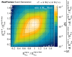
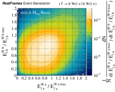
Refer to caption
Refer to caption
Refer to caption
Refer to caption
Refer to caption
Refer to caption
Figure 22: Distributions of (a) Ebatasuperscriptsubscript𝐸subscript𝑏𝑎subscript𝑡𝑎E_{\footnotesize\mathrm{{\color[rgb]{0.1,0.1,0.44}\definecolor[named]{pgfstrokecolor}{rgb}{0.1,0.1,0.44}\textbf{$b_{a}$}}}}^{\footnotesize\leavevmode\nobreak\ \mathrm{{\color[rgb]{0.45,0.0,0.09}\definecolor[named]{pgfstrokecolor}{rgb}{0.45,0.0,0.09}\textbf{$t_{a}$}}}} vs. Ebbtbsuperscriptsubscript𝐸subscript𝑏𝑏subscript𝑡𝑏E_{\footnotesize\mathrm{{\color[rgb]{0.1,0.1,0.44}\definecolor[named]{pgfstrokecolor}{rgb}{0.1,0.1,0.44}\textbf{$b_{b}$}}}}^{\footnotesize\leavevmode\nobreak\ \mathrm{{\color[rgb]{0.45,0.0,0.09}\definecolor[named]{pgfstrokecolor}{rgb}{0.45,0.0,0.09}\textbf{$t_{b}$}}}}, (b) EaWasuperscriptsubscript𝐸subscript𝑎subscript𝑊𝑎E_{\footnotesize\mathrm{{\color[rgb]{0.1,0.1,0.44}\definecolor[named]{pgfstrokecolor}{rgb}{0.1,0.1,0.44}\textbf{$\ell_{a}$}}}}^{\footnotesize\leavevmode\nobreak\ \mathrm{{\color[rgb]{0.45,0.0,0.09}\definecolor[named]{pgfstrokecolor}{rgb}{0.45,0.0,0.09}\textbf{$W_{a}$}}}} vs. EbWbsuperscriptsubscript𝐸subscript𝑏subscript𝑊𝑏E_{\footnotesize\mathrm{{\color[rgb]{0.1,0.1,0.44}\definecolor[named]{pgfstrokecolor}{rgb}{0.1,0.1,0.44}\textbf{$\ell_{b}$}}}}^{\footnotesize\leavevmode\nobreak\ \mathrm{{\color[rgb]{0.45,0.0,0.09}\definecolor[named]{pgfstrokecolor}{rgb}{0.45,0.0,0.09}\textbf{$W_{b}$}}}}, (c) Ebatasuperscriptsubscript𝐸subscript𝑏𝑎subscript𝑡𝑎E_{\footnotesize\mathrm{{\color[rgb]{0.1,0.1,0.44}\definecolor[named]{pgfstrokecolor}{rgb}{0.1,0.1,0.44}\textbf{$b_{a}$}}}}^{\footnotesize\leavevmode\nobreak\ \mathrm{{\color[rgb]{0.45,0.0,0.09}\definecolor[named]{pgfstrokecolor}{rgb}{0.45,0.0,0.09}\textbf{$t_{a}$}}}} vs. EaWasuperscriptsubscript𝐸subscript𝑎subscript𝑊𝑎E_{\footnotesize\mathrm{{\color[rgb]{0.1,0.1,0.44}\definecolor[named]{pgfstrokecolor}{rgb}{0.1,0.1,0.44}\textbf{$\ell_{a}$}}}}^{\footnotesize\leavevmode\nobreak\ \mathrm{{\color[rgb]{0.45,0.0,0.09}\definecolor[named]{pgfstrokecolor}{rgb}{0.45,0.0,0.09}\textbf{$W_{a}$}}}}, (d) θtasubscript𝜃subscript𝑡𝑎\theta_{\mathrm{{\color[rgb]{0.45,0.0,0.09}\definecolor[named]{pgfstrokecolor}{rgb}{0.45,0.0,0.09}\textbf{$t_{a}$}}}} vs. θtbsubscript𝜃subscript𝑡𝑏\theta_{\mathrm{{\color[rgb]{0.45,0.0,0.09}\definecolor[named]{pgfstrokecolor}{rgb}{0.45,0.0,0.09}\textbf{$t_{b}$}}}}, (e) θWasubscript𝜃subscript𝑊𝑎\theta_{\mathrm{{\color[rgb]{0.45,0.0,0.09}\definecolor[named]{pgfstrokecolor}{rgb}{0.45,0.0,0.09}\textbf{$W_{a}$}}}} vs. θWbsubscript𝜃subscript𝑊𝑏\theta_{\mathrm{{\color[rgb]{0.45,0.0,0.09}\definecolor[named]{pgfstrokecolor}{rgb}{0.45,0.0,0.09}\textbf{$W_{b}$}}}}, and (f) θtasubscript𝜃subscript𝑡𝑎\theta_{\mathrm{{\color[rgb]{0.45,0.0,0.09}\definecolor[named]{pgfstrokecolor}{rgb}{0.45,0.0,0.09}\textbf{$t_{a}$}}}} vs. θWasubscript𝜃subscript𝑊𝑎\theta_{\mathrm{{\color[rgb]{0.45,0.0,0.09}\definecolor[named]{pgfstrokecolor}{rgb}{0.45,0.0,0.09}\textbf{$W_{a}$}}}} in simulated tt¯bW(ν)bW(ν)𝑡¯𝑡𝑏𝑊𝜈𝑏𝑊𝜈t\bar{t}\rightarrow bW(\ell\nu)bW(\ell\nu) events at a hadron collider, calculated using the min ΔMtopΔsubscript𝑀top\Delta M_{\rm top}\leavevmode\nobreak\ approach. Each observable is normalized appropriately by the true value of the quantity it is estimating, with angles shown in units radian.

Corresponding distributions of the correlations between the top and W𝑊W decay angles for each half of the event, shown in Fig. 22, confirm the near independence of the observables corresponding to different reference frames, with each estimating their respective true values accurately. In addition to the observables describing the mass and decay of the di-top system, which are studied in the following example, the total set of derived estimators in an RJR scheme like min ΔMtopΔsubscript𝑀top\Delta M_{\rm top}\leavevmode\nobreak\ constitute an excellent basis for studying these events, with only small correlations and uniformly good resolution of a collection of quantities, including masses and spin-sensitive decay angles.

VII.2 H0tt¯bW(ν)bW(ν)superscript𝐻0𝑡¯𝑡𝑏𝑊𝜈𝑏𝑊𝜈H^{0}\rightarrow{t}\bar{t}\rightarrow bW(\ell\nu)bW(\ell\nu)

We continue our discussion of di-leptonic tt¯𝑡¯𝑡t\bar{t} final states by considering resonant top pair production, through a heavy, neutral Higgs boson, H0superscript𝐻0H^{0}. The kinematics of the decay tree describing this final state, shown in Fig. 23, is identical to that of the previous example, with four visible particles accompanied by two neutrinos. We will adopt the notation of Section VII.1 throughout this example.
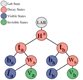
Refer to caption
Figure 23: A decay tree for a heavy, neutral Higgs boson decaying to a tt¯𝑡¯𝑡t\bar{t} pair, each of which decays to a b𝑏b-quark and W(ν)𝑊𝜈W(\ell\nu).

While for non-resonant top pair production we focused on the reconstruction of the top and W𝑊W rest frames, along with their associated estimators, here we are primarily interested in the approximation of the Higgs rest frame, its mass, and decay angles. In order to minimize any bias in the Higgs mass estimator, MH0superscriptsubscript𝑀superscript𝐻0absentM_{\footnotesize\mathrm{{\color[rgb]{0.45,0.0,0.09}\definecolor[named]{pgfstrokecolor}{rgb}{0.45,0.0,0.09}\textbf{$H^{0}$}}}}^{\footnotesize\leavevmode\nobreak\ }, we adopt the min ΔMtopΔsubscript𝑀top\Delta M_{\rm top}\leavevmode\nobreak\ scheme, described in Section VII.1, for analyzing events in this example, which allows us to fix the individual neutrino masses to zero. This approach applies the Lorentz invariant choice for the total mass of the di-neutrino system MI=2|pa/b|superscriptsubscript𝑀Iabsent2superscriptsubscript𝑝subscript𝑎𝑏M_{\footnotesize\mathrm{{\color[rgb]{0.12,0.3,0.17}\definecolor[named]{pgfstrokecolor}{rgb}{0.12,0.3,0.17}\textbf{I}}}}^{\footnotesize\leavevmode\nobreak\ }=2|\vec{p}_{\footnotesize\mathrm{{\color[rgb]{0.1,0.1,0.44}\definecolor[named]{pgfstrokecolor}{rgb}{0.1,0.1,0.44}\textbf{$\ell_{a/b}$}}}}^{\footnotesize\leavevmode\nobreak\ \mathrm{{\color[rgb]{0.1,0.1,0.44}\definecolor[named]{pgfstrokecolor}{rgb}{0.1,0.1,0.44}\textbf{$\ell\ell$}}}}|, exploiting the symmetry of the neutrinos and leptons in their production.

The distribution of MH0superscriptsubscript𝑀superscript𝐻0absentM_{\footnotesize\mathrm{{\color[rgb]{0.45,0.0,0.09}\definecolor[named]{pgfstrokecolor}{rgb}{0.45,0.0,0.09}\textbf{$H^{0}$}}}}^{\footnotesize\leavevmode\nobreak\ }, for varying Higgs boson mass, is shown for simulated H0tt¯bW(ν)bW(ν)superscript𝐻0𝑡¯𝑡𝑏𝑊𝜈𝑏𝑊𝜈H^{0}\rightarrow{t}\bar{t}\rightarrow bW(\ell\nu)bW(\ell\nu) events in Fig. 24, where the observable peaks at the true value of the mass it is estimating with roughly constant relative resolution. This is indicative that, on average, our guess for the neutrino system’s contribution to the Higgs mass is unbiased and not wholly inaccurate.
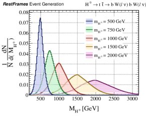
Refer to caption
Figure 24: Distribution of the Higgs boson mass estimator, MH0superscriptsubscript𝑀superscript𝐻0absentM_{\footnotesize\mathrm{{\color[rgb]{0.45,0.0,0.09}\definecolor[named]{pgfstrokecolor}{rgb}{0.45,0.0,0.09}\textbf{$H^{0}$}}}}^{\footnotesize\leavevmode\nobreak\ }, in simulated H0tt¯bW(ν)bW(ν)superscript𝐻0𝑡¯𝑡𝑏𝑊𝜈𝑏𝑊𝜈H^{0}\rightarrow{t}\bar{t}\rightarrow bW(\ell\nu)bW(\ell\nu) events with varying Higgs mass.

MH0superscriptsubscript𝑀superscript𝐻0absentM_{\footnotesize\mathrm{{\color[rgb]{0.45,0.0,0.09}\definecolor[named]{pgfstrokecolor}{rgb}{0.45,0.0,0.09}\textbf{$H^{0}$}}}}^{\footnotesize\leavevmode\nobreak\ } estimates the Higgs boson mass with 1720%similar-toabsent17percent20\sim 17-20\% resolution for those considered in this study, degrading with increasing mass, as demonstrated in Fig. 25(a). With this accuracy, the reconstructed MH0superscriptsubscript𝑀superscript𝐻0absentM_{\footnotesize\mathrm{{\color[rgb]{0.45,0.0,0.09}\definecolor[named]{pgfstrokecolor}{rgb}{0.45,0.0,0.09}\textbf{$H^{0}$}}}}^{\footnotesize\leavevmode\nobreak\ } has a width comparable to that in fully hadronic tt¯𝑡¯𝑡t\bar{t} final states, with contributions from jet momentum and mass uncertainty resulting in a similar value.
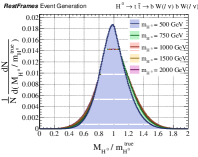
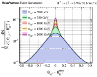
Refer to caption
Refer to caption
Figure 25: Distributions of (a) the Higgs boson mass estimator, MH0superscriptsubscript𝑀superscript𝐻0absentM_{\footnotesize\mathrm{{\color[rgb]{0.45,0.0,0.09}\definecolor[named]{pgfstrokecolor}{rgb}{0.45,0.0,0.09}\textbf{$H^{0}$}}}}^{\footnotesize\leavevmode\nobreak\ }, and (b) θH0subscript𝜃superscript𝐻0\theta_{\mathrm{{\color[rgb]{0.45,0.0,0.09}\definecolor[named]{pgfstrokecolor}{rgb}{0.45,0.0,0.09}\textbf{$H^{0}$}}}} in simulated H0tt¯bW(ν)bW(ν)superscript𝐻0𝑡¯𝑡𝑏𝑊𝜈𝑏𝑊𝜈H^{0}\rightarrow{t}\bar{t}\rightarrow bW(\ell\nu)bW(\ell\nu) events with varying Higgs mass. Each observable is appropriately normalized by the true value of the quantity it is estimating, with angles in units radian.

Conversely, the resolution of the Higgs decay angle estimator, θH0subscript𝜃superscript𝐻0\theta_{\mathrm{{\color[rgb]{0.45,0.0,0.09}\definecolor[named]{pgfstrokecolor}{rgb}{0.45,0.0,0.09}\textbf{$H^{0}$}}}}, improves with increasing Higgs mass, as can be seen in Fig. 25(b). This is indicative of the fact that as the velocity of the top quarks increases in the Higgs rest frame, the estimate of the magnitude of that velocity (related to MH0superscriptsubscript𝑀superscript𝐻0absentM_{\footnotesize\mathrm{{\color[rgb]{0.45,0.0,0.09}\definecolor[named]{pgfstrokecolor}{rgb}{0.45,0.0,0.09}\textbf{$H^{0}$}}}}^{\footnotesize\leavevmode\nobreak\ }) becomes more uncertain while it’s direction (related to θH0subscript𝜃superscript𝐻0\theta_{\mathrm{{\color[rgb]{0.45,0.0,0.09}\definecolor[named]{pgfstrokecolor}{rgb}{0.45,0.0,0.09}\textbf{$H^{0}$}}}}) is better resolved.

This mild dependency of the βtaH0superscriptsubscript𝛽subscript𝑡𝑎superscript𝐻0\vec{\beta}_{\footnotesize\mathrm{{\color[rgb]{0.45,0.0,0.09}\definecolor[named]{pgfstrokecolor}{rgb}{0.45,0.0,0.09}\textbf{$t_{a}$}}}}^{\footnotesize\leavevmode\nobreak\ \mathrm{{\color[rgb]{0.45,0.0,0.09}\definecolor[named]{pgfstrokecolor}{rgb}{0.45,0.0,0.09}\textbf{$H^{0}$}}}} estimate on the Higgs mass also has implications for the reconstruction of the top and W𝑊W rest frames. The distributions of the b𝑏b-tagged jet and lepton energies in the approximations of their respective production frames are shown in Fig. 26. As the velocity relating the Higgs rest frame to the tops’ respective rest frames becomes more uncertain, the resolution of these reference frames degrades, with corresponding effects on the observables associated with them. These higher order reconstruction effects, resulting from mis-measurements of the velocities relating different reference frames in a decay tree, introduce many of the small correlations observed between estimators in the RJR approach.
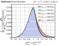
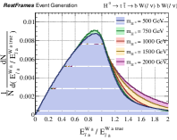
Refer to caption
Refer to caption
Figure 26: Distributions of (a) the reconstructed energy of a b𝑏b-tagged jet in the approximation of its production frame, Ebatasuperscriptsubscript𝐸subscript𝑏𝑎subscript𝑡𝑎E_{\footnotesize\mathrm{{\color[rgb]{0.1,0.1,0.44}\definecolor[named]{pgfstrokecolor}{rgb}{0.1,0.1,0.44}\textbf{$b_{a}$}}}}^{\footnotesize\leavevmode\nobreak\ \mathrm{{\color[rgb]{0.45,0.0,0.09}\definecolor[named]{pgfstrokecolor}{rgb}{0.45,0.0,0.09}\textbf{$t_{a}$}}}}, and (b) EaWasuperscriptsubscript𝐸subscript𝑎subscript𝑊𝑎E_{\footnotesize\mathrm{{\color[rgb]{0.1,0.1,0.44}\definecolor[named]{pgfstrokecolor}{rgb}{0.1,0.1,0.44}\textbf{$\ell_{a}$}}}}^{\footnotesize\leavevmode\nobreak\ \mathrm{{\color[rgb]{0.45,0.0,0.09}\definecolor[named]{pgfstrokecolor}{rgb}{0.45,0.0,0.09}\textbf{$W_{a}$}}}} in simulated H0tt¯bW(ν)bW(ν)superscript𝐻0𝑡¯𝑡𝑏𝑊𝜈𝑏𝑊𝜈H^{0}\rightarrow{t}\bar{t}\rightarrow bW(\ell\nu)bW(\ell\nu) events with varying Higgs mass. Each observable is appropriately normalized by the true value of the quantity it is estimating.

The magnitude of these residual correlations on the estimates of the visible particle energies in their production frames can be observed when considering their dependence on the reconstructed Higgs boson mass, as can be seen in Fig. 27(a,b) for simulated events with mH0=1superscriptsubscript𝑚superscript𝐻0absent1m_{\footnotesize\mathrm{{\color[rgb]{0.45,0.0,0.09}\definecolor[named]{pgfstrokecolor}{rgb}{0.45,0.0,0.09}\textbf{$H^{0}$}}}}^{\footnotesize\leavevmode\nobreak\ }=1 TeV. The observables have small correlations, comparable to those between the visible energy estimators themselves as seen previously in Section VII.1.
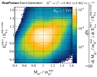
Refer to caption
Refer to caption
Refer to caption
Refer to caption
Figure 27: Distributions of (a) Ebatasuperscriptsubscript𝐸subscript𝑏𝑎subscript𝑡𝑎E_{\footnotesize\mathrm{{\color[rgb]{0.1,0.1,0.44}\definecolor[named]{pgfstrokecolor}{rgb}{0.1,0.1,0.44}\textbf{$b_{a}$}}}}^{\footnotesize\leavevmode\nobreak\ \mathrm{{\color[rgb]{0.45,0.0,0.09}\definecolor[named]{pgfstrokecolor}{rgb}{0.45,0.0,0.09}\textbf{$t_{a}$}}}}, and (b) EaWasuperscriptsubscript𝐸subscript𝑎subscript𝑊𝑎E_{\footnotesize\mathrm{{\color[rgb]{0.1,0.1,0.44}\definecolor[named]{pgfstrokecolor}{rgb}{0.1,0.1,0.44}\textbf{$\ell_{a}$}}}}^{\footnotesize\leavevmode\nobreak\ \mathrm{{\color[rgb]{0.45,0.0,0.09}\definecolor[named]{pgfstrokecolor}{rgb}{0.45,0.0,0.09}\textbf{$W_{a}$}}}}, as a function of MH0superscriptsubscript𝑀superscript𝐻0absentM_{\footnotesize\mathrm{{\color[rgb]{0.45,0.0,0.09}\definecolor[named]{pgfstrokecolor}{rgb}{0.45,0.0,0.09}\textbf{$H^{0}$}}}}^{\footnotesize\leavevmode\nobreak\ }, and (c) θtasubscript𝜃subscript𝑡𝑎\theta_{\mathrm{{\color[rgb]{0.45,0.0,0.09}\definecolor[named]{pgfstrokecolor}{rgb}{0.45,0.0,0.09}\textbf{$t_{a}$}}}}, and (d) θWasubscript𝜃subscript𝑊𝑎\theta_{\mathrm{{\color[rgb]{0.45,0.0,0.09}\definecolor[named]{pgfstrokecolor}{rgb}{0.45,0.0,0.09}\textbf{$W_{a}$}}}}, as a function of θHsubscript𝜃𝐻\theta_{\mathrm{{\color[rgb]{0.45,0.0,0.09}\definecolor[named]{pgfstrokecolor}{rgb}{0.45,0.0,0.09}\textbf{$H$}}}}, in simulated H0tt¯bW(ν)bW(ν)superscript𝐻0𝑡¯𝑡𝑏𝑊𝜈𝑏𝑊𝜈H^{0}\rightarrow{t}\bar{t}\rightarrow bW(\ell\nu)bW(\ell\nu) events. The true Higgs mass is set to mH0=1superscriptsubscript𝑚superscript𝐻0absent1m_{\footnotesize\mathrm{{\color[rgb]{0.45,0.0,0.09}\definecolor[named]{pgfstrokecolor}{rgb}{0.45,0.0,0.09}\textbf{$H^{0}$}}}}^{\footnotesize\leavevmode\nobreak\ }=1 TeV. Each observable is normalized by the true value, with angles in units radian.

A similar conclusion holds when considering the dependence of the top and W𝑊W decay angle estimators on the analogous quantity for the Higgs, as demonstrated in Fig. 27(c,d), where the observables exhibit negligible correlation. Taken with the conclusions from the previous example, it is clear that the estimators calculated in the RJR approach for this final state, in a particular reference frame, are almost entirely independent of those associated with different frames, with the accuracy of each of the estimators remaining stable - a crucial property of this basis of observables.

VII.3 t~t~bχ~1±(ν~)bχ~1(ν~)~𝑡~𝑡𝑏superscriptsubscript~𝜒1plus-or-minus~𝜈𝑏superscriptsubscript~𝜒1minus-or-plus~𝜈\tilde{t}\tilde{t}\rightarrow b\tilde{\chi}_{1}^{\pm}(\ell\tilde{\nu})b\tilde{\chi}_{1}^{\mp}(\ell\tilde{\nu}) at a hadron collider

The final permutation of final states with two leptons, two b𝑏b-tagged jets, and two invisible particles we consider is the case of stop quark pair production at a hadron collider, where each stop decays to a b𝑏b-quark and chargino which, in turn, decays to a lepton and a sneutrino. We assume that the sneutrino is either the lightest supersymmetric particle or that it decays via ν~νχ~10~𝜈𝜈subscriptsuperscript~𝜒01\tilde{\nu}\rightarrow\nu\tilde{\chi}^{0}_{1}, such that it behaves as an individual invisible particle. The decay tree diagram for this final state, shown in Fig. 28, is identical to that for fully-leptonic top pair production, with the intermediate particle states and invisible particles replaced by their supersymmetric counterparts.
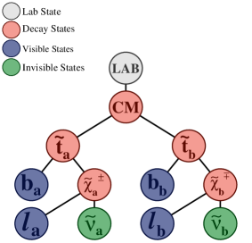
Refer to caption
Figure 28: Decay tree for stop pair production with decays to b𝑏b-quarks, leptons, and sneutrinos, via a chargino. While the stop quarks and sneutrinos are assumed to have the same mass in each half of the event, the charginos may correspond to different mass eigenstates.

The appeal of the RJR approach for studying events like these is that one can estimate the mass splittings of these particles and, in cases with many intermediate masses, do so largely independently of each other. The same strategy can be used whether the chargino appearing in these events has a mass degenerate with the stop, nearly as small as the sneutrino, or anywhere in between. In the context of a search for evidence of this phenomenon, this mass sensitivity is essential for distinguishing this process from a likely large tt¯𝑡¯𝑡t\bar{t} background, where one or more mass splittings may be similar their SM counterparts, and difficult to distinguish from them.

If one were attempting to study the spin correlations of these stop decays, unbiased estimations of the total di-stop invariant mass and decay angles would be valuable, such that the min ΔMtopΔsubscript𝑀top\Delta M_{\rm top}\leavevmode\nobreak\ analysis scheme described in Section VII.1 would be appropriate. In a discovery search, these observables are less relevant, with estimation of the intermediate particle mass splittings a higher priority. Recalling that the Mtopa=Mtopbsuperscriptsubscript𝑀top𝑎superscriptsubscript𝑀top𝑏M_{\rm top}^{a}=M_{\rm top}^{b}\leavevmode\nobreak\ approach of Section VII.1 provided the most accurate, and least biased, estimators of the relevant mass splittings, Eba/bt~a/bsuperscriptsubscript𝐸subscript𝑏𝑎𝑏subscript~𝑡𝑎𝑏E_{\footnotesize\mathrm{{\color[rgb]{0.1,0.1,0.44}\definecolor[named]{pgfstrokecolor}{rgb}{0.1,0.1,0.44}\textbf{$b_{a/b}$}}}}^{\footnotesize\leavevmode\nobreak\ \mathrm{{\color[rgb]{0.45,0.0,0.09}\definecolor[named]{pgfstrokecolor}{rgb}{0.45,0.0,0.09}\textbf{$\tilde{t}_{a/b}$}}}} and Ea/bχ~a/b±superscriptsubscript𝐸subscript𝑎𝑏subscriptsuperscript~𝜒plus-or-minus𝑎𝑏E_{\footnotesize\mathrm{{\color[rgb]{0.1,0.1,0.44}\definecolor[named]{pgfstrokecolor}{rgb}{0.1,0.1,0.44}\textbf{$\ell_{a/b}$}}}}^{\footnotesize\leavevmode\nobreak\ \mathrm{{\color[rgb]{0.45,0.0,0.09}\definecolor[named]{pgfstrokecolor}{rgb}{0.45,0.0,0.09}\textbf{$\tilde{\chi}^{\pm}_{a/b}$}}}}, we adopt that strategy for the analysis of t~t~bχ~1±(ν~)bχ~1(ν~)~𝑡~𝑡𝑏superscriptsubscript~𝜒1plus-or-minus~𝜈𝑏superscriptsubscript~𝜒1minus-or-plus~𝜈\tilde{t}\tilde{t}\rightarrow b\tilde{\chi}_{1}^{\pm}(\ell\tilde{\nu})b\tilde{\chi}_{1}^{\mp}(\ell\tilde{\nu}).

While the absolute values of the mass differences between the stop, chargino, and sneutrino may differ from their SM analogues, the behavior of the RJR observables, when compared with the true quantities we are attempting to estimate in these events, depends primarily on the ratio of the mass splittings in each decay step. We imagine in this example that each stop quark has mt~=800superscriptsubscript𝑚~𝑡absent800m_{\footnotesize\mathrm{{\color[rgb]{0.45,0.0,0.09}\definecolor[named]{pgfstrokecolor}{rgb}{0.45,0.0,0.09}\textbf{$\tilde{t}$}}}}^{\footnotesize\leavevmode\nobreak\ }=800 GeV, and each sneutrino mν~=100superscriptsubscript𝑚~𝜈absent100m_{\footnotesize\mathrm{{\color[rgb]{0.12,0.3,0.17}\definecolor[named]{pgfstrokecolor}{rgb}{0.12,0.3,0.17}\textbf{$\tilde{\nu}$}}}}^{\footnotesize\leavevmode\nobreak\ }=100 GeV. A range of intermediate chargino masses are considered, parameterized by the ratio of chargino/sneutrino and stop/sneutrino mass differences, Rmχ~±subscript𝑅superscriptsubscript𝑚superscript~𝜒plus-or-minusabsentR_{m_{\footnotesize\tilde{\chi}^{\pm}}^{\footnotesize\leavevmode\nobreak\ }}:

Rmχ~±=mχ~±mν~mt~mν~.subscript𝑅superscriptsubscript𝑚superscript~𝜒plus-or-minusabsentsuperscriptsubscript𝑚superscript~𝜒plus-or-minusabsentsuperscriptsubscript𝑚~𝜈absentsuperscriptsubscript𝑚~𝑡absentsuperscriptsubscript𝑚~𝜈absent\displaystyle R_{m_{\footnotesize\tilde{\chi}^{\pm}}^{\footnotesize\leavevmode\nobreak\ }}=\frac{m_{\footnotesize\mathrm{{\color[rgb]{0.45,0.0,0.09}\definecolor[named]{pgfstrokecolor}{rgb}{0.45,0.0,0.09}\textbf{$\tilde{\chi}^{\pm}$}}}}^{\footnotesize\leavevmode\nobreak\ }-m_{\footnotesize\mathrm{{\color[rgb]{0.12,0.3,0.17}\definecolor[named]{pgfstrokecolor}{rgb}{0.12,0.3,0.17}\textbf{$\tilde{\nu}$}}}}^{\footnotesize\leavevmode\nobreak\ }}{m_{\footnotesize\mathrm{{\color[rgb]{0.45,0.0,0.09}\definecolor[named]{pgfstrokecolor}{rgb}{0.45,0.0,0.09}\textbf{$\tilde{t}$}}}}^{\footnotesize\leavevmode\nobreak\ }-m_{\footnotesize\mathrm{{\color[rgb]{0.12,0.3,0.17}\definecolor[named]{pgfstrokecolor}{rgb}{0.12,0.3,0.17}\textbf{$\tilde{\nu}$}}}}^{\footnotesize\leavevmode\nobreak\ }}\leavevmode\nobreak\ . (61)

The distributions of the visible particle energy estimators, Ebat~superscriptsubscript𝐸subscript𝑏𝑎~𝑡E_{\footnotesize\mathrm{{\color[rgb]{0.1,0.1,0.44}\definecolor[named]{pgfstrokecolor}{rgb}{0.1,0.1,0.44}\textbf{$b_{a}$}}}}^{\footnotesize\leavevmode\nobreak\ \mathrm{{\color[rgb]{0.45,0.0,0.09}\definecolor[named]{pgfstrokecolor}{rgb}{0.45,0.0,0.09}\textbf{$\tilde{t}$}}}} and Eaχ~a±superscriptsubscript𝐸subscript𝑎subscriptsuperscript~𝜒plus-or-minus𝑎E_{\footnotesize\mathrm{{\color[rgb]{0.1,0.1,0.44}\definecolor[named]{pgfstrokecolor}{rgb}{0.1,0.1,0.44}\textbf{$\ell_{a}$}}}}^{\footnotesize\leavevmode\nobreak\ \mathrm{{\color[rgb]{0.45,0.0,0.09}\definecolor[named]{pgfstrokecolor}{rgb}{0.45,0.0,0.09}\textbf{$\tilde{\chi}^{\pm}_{a}$}}}}, and the reconstructed stop decay angle are shown, as a function of Rmχ~±subscript𝑅superscriptsubscript𝑚superscript~𝜒plus-or-minusabsentR_{m_{\footnotesize\tilde{\chi}^{\pm}}^{\footnotesize\leavevmode\nobreak\ }}, for simulated events in Fig. 29(a,b,c), where the true values of the chargino masses mχ~a±=mχ~b±superscriptsubscript𝑚subscriptsuperscript~𝜒plus-or-minus𝑎absentsuperscriptsubscript𝑚subscriptsuperscript~𝜒plus-or-minus𝑏absentm_{\footnotesize\mathrm{{\color[rgb]{0.45,0.0,0.09}\definecolor[named]{pgfstrokecolor}{rgb}{0.45,0.0,0.09}\textbf{$\tilde{\chi}^{\pm}_{a}$}}}}^{\footnotesize\leavevmode\nobreak\ }=m_{\footnotesize\mathrm{{\color[rgb]{0.45,0.0,0.09}\definecolor[named]{pgfstrokecolor}{rgb}{0.45,0.0,0.09}\textbf{$\tilde{\chi}^{\pm}_{b}$}}}}^{\footnotesize\leavevmode\nobreak\ } are varied between their kinematically allowed values. As Rmχ~±0subscript𝑅superscriptsubscript𝑚superscript~𝜒plus-or-minusabsent0R_{m_{\footnotesize\tilde{\chi}^{\pm}}^{\footnotesize\leavevmode\nobreak\ }}\rightarrow 0, the phase-space in the production of the lepton becomes negligible, meaning these events appear as if the stop quarks are decaying as t~t~bν~bν~~𝑡~𝑡𝑏~𝜈𝑏~𝜈\tilde{t}\tilde{t}\rightarrow b\tilde{\nu}b\tilde{\nu}. This results in the Ebat~superscriptsubscript𝐸subscript𝑏𝑎~𝑡E_{\footnotesize\mathrm{{\color[rgb]{0.1,0.1,0.44}\definecolor[named]{pgfstrokecolor}{rgb}{0.1,0.1,0.44}\textbf{$b_{a}$}}}}^{\footnotesize\leavevmode\nobreak\ \mathrm{{\color[rgb]{0.45,0.0,0.09}\definecolor[named]{pgfstrokecolor}{rgb}{0.45,0.0,0.09}\textbf{$\tilde{t}$}}}} distribution exhibiting a kinematic edge at the true value, similar to the analogous quantity shown in Fig. 15 for t~t~thadχ~10thadχ~10~𝑡~𝑡subscript𝑡hadsubscriptsuperscript~𝜒01subscript𝑡hadsubscriptsuperscript~𝜒01\tilde{t}\tilde{t}\rightarrow t_{\rm had}\tilde{\chi}^{0}_{1}t_{\rm had}\tilde{\chi}^{0}_{1} events. Conversely, as Rmχ~±1subscript𝑅superscriptsubscript𝑚superscript~𝜒plus-or-minusabsent1R_{m_{\footnotesize\tilde{\chi}^{\pm}}^{\footnotesize\leavevmode\nobreak\ }}\rightarrow 1 the events appear as if the stops are decaying t~t~ν~ν~~𝑡~𝑡~𝜈~𝜈\tilde{t}\tilde{t}\rightarrow\ell\tilde{\nu}\ell\tilde{\nu}, with the Eaχ~a±superscriptsubscript𝐸subscript𝑎subscriptsuperscript~𝜒plus-or-minus𝑎E_{\footnotesize\mathrm{{\color[rgb]{0.1,0.1,0.44}\definecolor[named]{pgfstrokecolor}{rgb}{0.1,0.1,0.44}\textbf{$\ell_{a}$}}}}^{\footnotesize\leavevmode\nobreak\ \mathrm{{\color[rgb]{0.45,0.0,0.09}\definecolor[named]{pgfstrokecolor}{rgb}{0.45,0.0,0.09}\textbf{$\tilde{\chi}^{\pm}_{a}$}}}} distribution in Fig. 29(b) taking a similar shape as for EaWasuperscriptsubscript𝐸subscript𝑎subscript𝑊𝑎E_{\footnotesize\mathrm{{\color[rgb]{0.1,0.1,0.44}\definecolor[named]{pgfstrokecolor}{rgb}{0.1,0.1,0.44}\textbf{$\ell_{a}$}}}}^{\footnotesize\leavevmode\nobreak\ \mathrm{{\color[rgb]{0.45,0.0,0.09}\definecolor[named]{pgfstrokecolor}{rgb}{0.45,0.0,0.09}\textbf{$W_{a}$}}}} in HW(ν)W(ν)𝐻𝑊𝜈𝑊𝜈H\rightarrow W(\ell\nu)W(\ell\nu) events from Fig. 11. As Rmχ~±subscript𝑅superscriptsubscript𝑚superscript~𝜒plus-or-minusabsentR_{m_{\footnotesize\tilde{\chi}^{\pm}}^{\footnotesize\leavevmode\nobreak\ }} approaches the opposite extremum for both energy estimators their distributions peak at the correct values, with increasingly degraded resolution as the associated decay phase-space shrinks. Similarly, the accuracy of the θt~asubscript𝜃subscript~𝑡𝑎\theta_{\mathrm{{\color[rgb]{0.45,0.0,0.09}\definecolor[named]{pgfstrokecolor}{rgb}{0.45,0.0,0.09}\textbf{$\tilde{t}_{a}$}}}} estimator becomes worse as the stop and chargino become degenerate in mass, developing a growing bias as this limit approaches, as can be seen in Fig. 29(c).
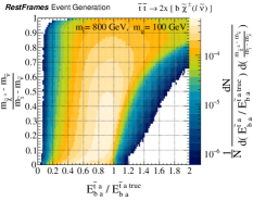
Refer to caption
Refer to caption
Refer to caption
Refer to caption
Refer to caption
Refer to caption
Figure 29: Distributions of (a,d) Ebat~asuperscriptsubscript𝐸subscript𝑏𝑎subscript~𝑡𝑎E_{\footnotesize\mathrm{{\color[rgb]{0.1,0.1,0.44}\definecolor[named]{pgfstrokecolor}{rgb}{0.1,0.1,0.44}\textbf{$b_{a}$}}}}^{\footnotesize\leavevmode\nobreak\ \mathrm{{\color[rgb]{0.45,0.0,0.09}\definecolor[named]{pgfstrokecolor}{rgb}{0.45,0.0,0.09}\textbf{$\tilde{t}_{a}$}}}}, (b,e) Eaχ~a±superscriptsubscript𝐸subscript𝑎subscriptsuperscript~𝜒plus-or-minus𝑎E_{\footnotesize\mathrm{{\color[rgb]{0.1,0.1,0.44}\definecolor[named]{pgfstrokecolor}{rgb}{0.1,0.1,0.44}\textbf{$\ell_{a}$}}}}^{\footnotesize\leavevmode\nobreak\ \mathrm{{\color[rgb]{0.45,0.0,0.09}\definecolor[named]{pgfstrokecolor}{rgb}{0.45,0.0,0.09}\textbf{$\tilde{\chi}^{\pm}_{a}$}}}}, and (c,f) θt~asubscript𝜃subscript~𝑡𝑎\theta_{\mathrm{{\color[rgb]{0.45,0.0,0.09}\definecolor[named]{pgfstrokecolor}{rgb}{0.45,0.0,0.09}\textbf{$\tilde{t}_{a}$}}}}, as a function of Rmχ~±subscript𝑅superscriptsubscript𝑚superscript~𝜒plus-or-minusabsentR_{m_{\footnotesize\tilde{\chi}^{\pm}}^{\footnotesize\leavevmode\nobreak\ }}, for simulated t~t~bχ~1±(ν~)bχ~1(ν~)~𝑡~𝑡𝑏superscriptsubscript~𝜒1plus-or-minus~𝜈𝑏superscriptsubscript~𝜒1minus-or-plus~𝜈\tilde{t}\tilde{t}\rightarrow b\tilde{\chi}_{1}^{\pm}(\ell\tilde{\nu})b\tilde{\chi}_{1}^{\mp}(\ell\tilde{\nu}) events. All observables are appropriately normalized by the true values they are estimating, with decay angles in units radian. The simulated stop and sneutrino masses are chosen as mt~=800superscriptsubscript𝑚~𝑡absent800m_{\footnotesize\mathrm{{\color[rgb]{0.45,0.0,0.09}\definecolor[named]{pgfstrokecolor}{rgb}{0.45,0.0,0.09}\textbf{$\tilde{t}$}}}}^{\footnotesize\leavevmode\nobreak\ }=800 GeV and mν~=100superscriptsubscript𝑚~𝜈absent100m_{\footnotesize\mathrm{{\color[rgb]{0.12,0.3,0.17}\definecolor[named]{pgfstrokecolor}{rgb}{0.12,0.3,0.17}\textbf{$\tilde{\nu}$}}}}^{\footnotesize\leavevmode\nobreak\ }=100 GeV, respectively. Figures (a,b,c) have mχ~a±=mχ~b±superscriptsubscript𝑚subscriptsuperscript~𝜒plus-or-minus𝑎absentsuperscriptsubscript𝑚subscriptsuperscript~𝜒plus-or-minus𝑏absentm_{\footnotesize\mathrm{{\color[rgb]{0.45,0.0,0.09}\definecolor[named]{pgfstrokecolor}{rgb}{0.45,0.0,0.09}\textbf{$\tilde{\chi}^{\pm}_{a}$}}}}^{\footnotesize\leavevmode\nobreak\ }=m_{\footnotesize\mathrm{{\color[rgb]{0.45,0.0,0.09}\definecolor[named]{pgfstrokecolor}{rgb}{0.45,0.0,0.09}\textbf{$\tilde{\chi}^{\pm}_{b}$}}}}^{\footnotesize\leavevmode\nobreak\ }, while figures (d,e,f) have one chargino mass fixed at mχ~b±=450superscriptsubscript𝑚subscriptsuperscript~𝜒plus-or-minus𝑏absent450m_{\footnotesize\mathrm{{\color[rgb]{0.45,0.0,0.09}\definecolor[named]{pgfstrokecolor}{rgb}{0.45,0.0,0.09}\textbf{$\tilde{\chi}^{\pm}_{b}$}}}}^{\footnotesize\leavevmode\nobreak\ }=450 GeV, and mχ~a±superscriptsubscript𝑚subscriptsuperscript~𝜒plus-or-minus𝑎absentm_{\footnotesize\mathrm{{\color[rgb]{0.45,0.0,0.09}\definecolor[named]{pgfstrokecolor}{rgb}{0.45,0.0,0.09}\textbf{$\tilde{\chi}^{\pm}_{a}$}}}}^{\footnotesize\leavevmode\nobreak\ } varying with Rmχ~±subscript𝑅superscriptsubscript𝑚superscript~𝜒plus-or-minusabsentR_{m_{\footnotesize\tilde{\chi}^{\pm}}^{\footnotesize\leavevmode\nobreak\ }}.

The RJR Mtopa=Mtopbsuperscriptsubscript𝑀top𝑎superscriptsubscript𝑀top𝑏M_{\rm top}^{a}=M_{\rm top}^{b}\leavevmode\nobreak\ approach is able to retain sensitivity to the true mass splittings between the sparticles in these events over a broad phase space of decays, even in the limit of degeneracy between masses. But the most remarkable property of the derived estimators is the level of independence observables sensitive to the different stop kinematics exhibit. If we imagine a case where there are two chargino mass eigenstates in between the stop and sneutrino masses, a single event could contain one of each of these charginos. To study what happens to the RJR estimators when these masses are different, we fix one chargino mass, with mχ~b±=450superscriptsubscript𝑚subscriptsuperscript~𝜒plus-or-minus𝑏absent450m_{\footnotesize\mathrm{{\color[rgb]{0.45,0.0,0.09}\definecolor[named]{pgfstrokecolor}{rgb}{0.45,0.0,0.09}\textbf{$\tilde{\chi}^{\pm}_{b}$}}}}^{\footnotesize\leavevmode\nobreak\ }=450 GeV, while varying the other over the allowable on-shell phase-space between the stop and sneutrino. The same estimators, Ebat~superscriptsubscript𝐸subscript𝑏𝑎~𝑡E_{\footnotesize\mathrm{{\color[rgb]{0.1,0.1,0.44}\definecolor[named]{pgfstrokecolor}{rgb}{0.1,0.1,0.44}\textbf{$b_{a}$}}}}^{\footnotesize\leavevmode\nobreak\ \mathrm{{\color[rgb]{0.45,0.0,0.09}\definecolor[named]{pgfstrokecolor}{rgb}{0.45,0.0,0.09}\textbf{$\tilde{t}$}}}}, Eaχ~a±superscriptsubscript𝐸subscript𝑎subscriptsuperscript~𝜒plus-or-minus𝑎E_{\footnotesize\mathrm{{\color[rgb]{0.1,0.1,0.44}\definecolor[named]{pgfstrokecolor}{rgb}{0.1,0.1,0.44}\textbf{$\ell_{a}$}}}}^{\footnotesize\leavevmode\nobreak\ \mathrm{{\color[rgb]{0.45,0.0,0.09}\definecolor[named]{pgfstrokecolor}{rgb}{0.45,0.0,0.09}\textbf{$\tilde{\chi}^{\pm}_{a}$}}}}, and θt~asubscript𝜃subscript~𝑡𝑎\theta_{\mathrm{{\color[rgb]{0.45,0.0,0.09}\definecolor[named]{pgfstrokecolor}{rgb}{0.45,0.0,0.09}\textbf{$\tilde{t}_{a}$}}}}, are shown as a function of Rmχ~±subscript𝑅superscriptsubscript𝑚superscript~𝜒plus-or-minusabsentR_{m_{\footnotesize\tilde{\chi}^{\pm}}^{\footnotesize\leavevmode\nobreak\ }} for this differing chargino mass scenario in Fig. 29(d,e,f). The similarities between the these distributions and those for mχ~a±=mχ~b±superscriptsubscript𝑚subscriptsuperscript~𝜒plus-or-minus𝑎absentsuperscriptsubscript𝑚subscriptsuperscript~𝜒plus-or-minus𝑏absentm_{\footnotesize\mathrm{{\color[rgb]{0.45,0.0,0.09}\definecolor[named]{pgfstrokecolor}{rgb}{0.45,0.0,0.09}\textbf{$\tilde{\chi}^{\pm}_{a}$}}}}^{\footnotesize\leavevmode\nobreak\ }=m_{\footnotesize\mathrm{{\color[rgb]{0.45,0.0,0.09}\definecolor[named]{pgfstrokecolor}{rgb}{0.45,0.0,0.09}\textbf{$\tilde{\chi}^{\pm}_{b}$}}}}^{\footnotesize\leavevmode\nobreak\ } in Fig. 29(a,b,c) are striking. With only small deformations, the estimators retain nearly identical dependence on Rmχ~±subscript𝑅superscriptsubscript𝑚superscript~𝜒plus-or-minusabsentR_{m_{\footnotesize\tilde{\chi}^{\pm}}^{\footnotesize\leavevmode\nobreak\ }} in the two cases, irrespective of the mass splittings of sparticles in the opposite half of the event. This independence between the two stops’ kinematics is a result of the application of the contra-boost invariant JR VI.4 when analyzing the event, making the observables associated with each stop insensitive to the true velocity relating its rest frame to its production frame and, hence, also the other stop. This means that one can effectively analyze each part of the event in approximate isolation, allowing for the recursive application of even more JR’s in events with additional kinematic structure, as is described in the following examples.

VIII Recursive Jigsaws For More Particles - Intermediate, Invisible, and Identical

The previous examples have introduced a large collection of configurable and interchangeable JR’s, which can be chosen to analyze a variety of events. As the decays we hope to study grow further in complexity, with additional invisible particles in the final state and higher degrees of combinatoric ambiguity, there are two treatments available. We can introduce further generalizations of existing JR’s to simultaneously choose more under-constrained degrees of freedom, an approach we discuss in Section VIII.1 for N2×W(ν)𝑁2𝑊𝜈N\geq 2\leavevmode\nobreak\ \times\leavevmode\nobreak\ W(\ell\nu) final states. Alternatively, we can combine existing JR’s, recursively, into logical trees, iteratively sub-dividing each event kinematically while choosing the appropriate degrees of freedom. The examples in Sections VIII.2 and VIII.3 demonstrate this latter approach, considering the processes Hhh4W(ν)𝐻4𝑊𝜈H\rightarrow hh\rightarrow 4W(\ell\nu) and g~g~bbχ~10bbχ~10~𝑔~𝑔𝑏𝑏subscriptsuperscript~𝜒01𝑏𝑏subscriptsuperscript~𝜒01\tilde{g}\tilde{g}\rightarrow bb\tilde{\chi}^{0}_{1}bb\tilde{\chi}^{0}_{1}. The additional JR’s defined in this section, combined with those described throughout this paper, constitute a sufficient collection for analyzing any final state, with an arbitrary degree of complexity and number unknowns.

VIII.1 ppN2×W(ν)pp𝑁2𝑊𝜈\mathrm{pp}\rightarrow N\geq 2\leavevmode\nobreak\ \times\leavevmode\nobreak\ W(\ell\nu)

As the number of invisible particles appearing in a final state increases, the number of unmeasured degrees of freedom grows quickly. If this increase is accompanied by additional mass constraints, for example between intermediate particles appearing in a decay, the additional unknowns can be mitigated with the recursive application of corresponding JR’s, exploiting the expected structure in each event to better resolve quantities of interest.

In some cases, additional complexity is not accompanied by more intermediate structure, with the number of unknowns growing much larger than the number of appropriate constraints. Such a case is the non-resonant production of N2𝑁2N\geq 2 W𝑊W bosons at a hadron collider, with each W𝑊W decaying to a lepton and a neutrino. The N=2𝑁2N=2 case corresponds to the example of HW(ν)W(ν)𝐻𝑊𝜈𝑊𝜈H\rightarrow W(\ell\nu)W(\ell\nu) production, described in Section VI.1. There, we used the constraint MWasuperscriptsubscript𝑀subscript𝑊𝑎absentM_{\footnotesize\mathrm{{\color[rgb]{0.45,0.0,0.09}\definecolor[named]{pgfstrokecolor}{rgb}{0.45,0.0,0.09}\textbf{$W_{a}$}}}}^{\footnotesize\leavevmode\nobreak\ } = MWbsuperscriptsubscript𝑀subscript𝑊𝑏absentM_{\footnotesize\mathrm{{\color[rgb]{0.45,0.0,0.09}\definecolor[named]{pgfstrokecolor}{rgb}{0.45,0.0,0.09}\textbf{$W_{b}$}}}}^{\footnotesize\leavevmode\nobreak\ } and the contra-boost invariant JR VI.4 to determine how to split the invisible system into two separate neutrinos, corresponding to the cm frame decay in the tree shown in Fig. 30(a). As we see for the N>2𝑁2N>2 decay trees in Fig. 30, the corresponding decay has an increasing number of legs, or velocities relating the cm frame to its daughter Wisubscript𝑊𝑖W_{i} systems’ rest frames, and hence a correspondingly larger number of unknowns, with additional neutrino four vectors to choose in the associated JR.
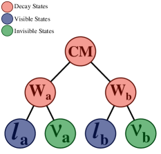
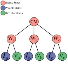
Refer to caption
Refer to caption
Refer to caption
Figure 30: Decay trees for ppN2×W(ν)pp𝑁2𝑊𝜈\mathrm{pp}\rightarrow N\geq 2\leavevmode\nobreak\ \times\leavevmode\nobreak\ W(\ell\nu) final states with (a) N=2𝑁2N=2, (b) N=3𝑁3N=3, and (c) N=4𝑁4N=4. The W𝑊W bosons are assumed to be produced non-resonantly, such that there is no phase-space structure beyond the flat N𝑁N-body phase space of the cm decay and subsequent W𝑊W decays. While they tend to have similar values in the RJR reconstruction of these events, the W𝑊W bosons are not explicitly constrained to have equal mass.

We assume that the N𝑁N leptons in the final state of each event are identified and reconstructed, with four vectors 𝐩ilabsuperscriptsubscript𝐩subscript𝑖lab\mathbf{p}_{\footnotesize\mathrm{{\color[rgb]{0.1,0.1,0.44}\definecolor[named]{pgfstrokecolor}{rgb}{0.1,0.1,0.44}\textbf{$\ell_{i}$}}}}^{\footnotesize\leavevmode\nobreak\ \mathrm{\textbf{lab}}}, and that the measurement of ETmisssuperscriptsubscript𝐸𝑇miss\vec{E}_{T}^{\rm miss}  in each event can be interpreted as the sum transverse momentum of the total invisible system of neutrinos, I={νi}Isubscript𝜈𝑖\mathrm{{\color[rgb]{0.12,0.3,0.17}\definecolor[named]{pgfstrokecolor}{rgb}{0.12,0.3,0.17}\textbf{I}}}=\{\mathrm{{\color[rgb]{0.12,0.3,0.17}\definecolor[named]{pgfstrokecolor}{rgb}{0.12,0.3,0.17}\textbf{$\nu_{i}$}}}\}, with pI,Tlab=ETmisssuperscriptsubscript𝑝I𝑇labsuperscriptsubscript𝐸𝑇miss\vec{p}_{\footnotesize\mathrm{{\color[rgb]{0.12,0.3,0.17}\definecolor[named]{pgfstrokecolor}{rgb}{0.12,0.3,0.17}\textbf{I}}},T}^{\footnotesize\leavevmode\nobreak\ \mathrm{\textbf{lab}}}=\vec{E}_{T}^{\rm miss}. With N𝑁N neutrino four vectors to resolve and only two constraints from the ETmisssuperscriptsubscript𝐸𝑇miss\vec{E}_{T}^{\rm miss}  measurement, there are 4N24𝑁24N-2 values left to choose.

As the W𝑊W bosons are expected to have different velocities in the cm frame when N3𝑁3N\geq 3, we are unable to introduce a generalization of contra-boost invariance for arbitrary N𝑁N. Applying direct mass constraints between the W𝑊W bosons can lead to multiple and/or complex solutions for kinematic quantities in events, and cannot be generalized to cases when the intermediate particle masses may be different. The shortcoming of simply choosing an inspired metric and minimizing it w.r.t. each of these unknowns simultaneously is that, with so many d.o.f., the minimization will be able to find small, trivial solutions. In order to resolve the fact that these events have intermediate structure in the form of massive W𝑊W bosons, we must either factorize the minimization of these unknowns (i.e. a binary decay tree) or perform the minimization with carefully constructed constraints to retain the structure. The algorithmic approach must also be tractable, in that the mass of the I system must be chosen as a Lorentz invariant function of the visible lepton four vectors, while the neutrinos’ masses must also obey any pre-determined constraints and remain non-tachyonic throughout the space of the minimization.

We adopt an ad-hoc approach inspired by the expected symmetry between the lepton and neutrino pairs’ four vectors due to their common provenance. In the derivation of JR VII.2, working in the rest frame of two invisible particles greatly simplified the problem, as their momentum was constrained to be equal and opposite, with a Lorentz invariant value, and only the orientation of this di-neutrino axis left to determine. Generalizing this concept, we choose the relative momentum of the neutrinos in the cm frame to correspond to that of the leptons in their respective V={i}Vsubscript𝑖\mathrm{{\color[rgb]{0.1,0.1,0.44}\definecolor[named]{pgfstrokecolor}{rgb}{0.1,0.1,0.44}\textbf{V}}}=\{\mathrm{{\color[rgb]{0.1,0.1,0.44}\definecolor[named]{pgfstrokecolor}{rgb}{0.1,0.1,0.44}\textbf{$\ell_{i}$}}}\} center-of-mass frame, such that

pνiI=𝐑(α,β,γ)piV,superscriptsubscript𝑝subscript𝜈𝑖I𝐑𝛼𝛽𝛾superscriptsubscript𝑝subscript𝑖V\displaystyle\vec{p}_{\footnotesize\mathrm{{\color[rgb]{0.12,0.3,0.17}\definecolor[named]{pgfstrokecolor}{rgb}{0.12,0.3,0.17}\textbf{$\nu_{i}$}}}}^{\footnotesize\leavevmode\nobreak\ \mathrm{{\color[rgb]{0.45,0.0,0.09}\definecolor[named]{pgfstrokecolor}{rgb}{0.45,0.0,0.09}\textbf{I}}}}=\mathbf{R}(\alpha,\beta,\gamma)\vec{p}_{\footnotesize\mathrm{{\color[rgb]{0.1,0.1,0.44}\definecolor[named]{pgfstrokecolor}{rgb}{0.1,0.1,0.44}\textbf{$\ell_{i}$}}}}^{\footnotesize\leavevmode\nobreak\ \mathrm{{\color[rgb]{0.45,0.0,0.09}\definecolor[named]{pgfstrokecolor}{rgb}{0.45,0.0,0.09}\textbf{V}}}}\leavevmode\nobreak\ , (62)

where 𝐑(α,β,γ)𝐑𝛼𝛽𝛾\mathbf{R}(\alpha,\beta,\gamma) is a 3×3333\times 3 dimensional rotation matrix described by the three Euler angles α𝛼\alpha, β𝛽\beta, and γ𝛾\gamma. With this constraint, we have reduced a potentially 3N33𝑁33N-3 d.o.f. minimization (assuming individual neutrino mass constraints) to 3, and are able to express our choice for MIsuperscriptsubscript𝑀IabsentM_{\footnotesize\mathrm{{\color[rgb]{0.12,0.3,0.17}\definecolor[named]{pgfstrokecolor}{rgb}{0.12,0.3,0.17}\textbf{I}}}}^{\footnotesize\leavevmode\nobreak\ } as a compatible Lorentz invariant expression:

MI=iN|piV|,superscriptsubscript𝑀Iabsentsuperscriptsubscript𝑖𝑁superscriptsubscript𝑝subscript𝑖V\displaystyle M_{\footnotesize\mathrm{{\color[rgb]{0.12,0.3,0.17}\definecolor[named]{pgfstrokecolor}{rgb}{0.12,0.3,0.17}\textbf{I}}}}^{\footnotesize\leavevmode\nobreak\ }=\sum_{i}^{N}|\vec{p}_{\footnotesize\mathrm{{\color[rgb]{0.1,0.1,0.44}\definecolor[named]{pgfstrokecolor}{rgb}{0.1,0.1,0.44}\textbf{$\ell_{i}$}}}}^{\footnotesize\leavevmode\nobreak\ \mathrm{{\color[rgb]{0.1,0.1,0.44}\definecolor[named]{pgfstrokecolor}{rgb}{0.1,0.1,0.44}\textbf{V}}}}|\leavevmode\nobreak\ , (63)

where we have constrained each Mνi=0superscriptsubscript𝑀subscript𝜈𝑖absent0M_{\footnotesize\mathrm{{\color[rgb]{0.12,0.3,0.17}\definecolor[named]{pgfstrokecolor}{rgb}{0.12,0.3,0.17}\textbf{$\nu_{i}$}}}}^{\footnotesize\leavevmode\nobreak\ }=0.

To determine the rotation 𝐑=𝐑(α,β,γ)𝐑𝐑𝛼𝛽𝛾\mathbf{R}=\mathbf{R}(\alpha,\beta,\gamma), we choose a metric with a linear dependence on the orientation of the neutrinos:

f(𝐑)𝑓𝐑\displaystyle f(\mathbf{R}) =\displaystyle= iNMWi 2superscriptsubscript𝑖𝑁superscriptsubscript𝑀subscript𝑊𝑖2\displaystyle\sum_{i}^{N}M_{\footnotesize\mathrm{{\color[rgb]{0.45,0.0,0.09}\definecolor[named]{pgfstrokecolor}{rgb}{0.45,0.0,0.09}\textbf{$W_{i}$}}}}^{\footnotesize\leavevmode\nobreak\ 2}
=\displaystyle= iN(mi 2+2(EiIEνiIpiIpνiI))superscriptsubscript𝑖𝑁superscriptsubscript𝑚subscript𝑖22superscriptsubscript𝐸subscript𝑖Isuperscriptsubscript𝐸subscript𝜈𝑖Isuperscriptsubscript𝑝subscript𝑖Isuperscriptsubscript𝑝subscript𝜈𝑖I\displaystyle\sum_{i}^{N}\left(m_{\footnotesize\mathrm{{\color[rgb]{0.1,0.1,0.44}\definecolor[named]{pgfstrokecolor}{rgb}{0.1,0.1,0.44}\textbf{$\ell_{i}$}}}}^{\footnotesize\leavevmode\nobreak\ 2}+2(E_{\footnotesize\mathrm{{\color[rgb]{0.1,0.1,0.44}\definecolor[named]{pgfstrokecolor}{rgb}{0.1,0.1,0.44}\textbf{$\ell_{i}$}}}}^{\footnotesize\leavevmode\nobreak\ \mathrm{{\color[rgb]{0.45,0.0,0.09}\definecolor[named]{pgfstrokecolor}{rgb}{0.45,0.0,0.09}\textbf{I}}}}E_{\footnotesize\mathrm{{\color[rgb]{0.12,0.3,0.17}\definecolor[named]{pgfstrokecolor}{rgb}{0.12,0.3,0.17}\textbf{$\nu_{i}$}}}}^{\footnotesize\leavevmode\nobreak\ \mathrm{{\color[rgb]{0.45,0.0,0.09}\definecolor[named]{pgfstrokecolor}{rgb}{0.45,0.0,0.09}\textbf{I}}}}-\vec{p}_{\footnotesize\mathrm{{\color[rgb]{0.1,0.1,0.44}\definecolor[named]{pgfstrokecolor}{rgb}{0.1,0.1,0.44}\textbf{$\ell_{i}$}}}}^{\footnotesize\leavevmode\nobreak\ \mathrm{{\color[rgb]{0.45,0.0,0.09}\definecolor[named]{pgfstrokecolor}{rgb}{0.45,0.0,0.09}\textbf{I}}}}\cdot\vec{p}_{\footnotesize\mathrm{{\color[rgb]{0.12,0.3,0.17}\definecolor[named]{pgfstrokecolor}{rgb}{0.12,0.3,0.17}\textbf{$\nu_{i}$}}}}^{\footnotesize\leavevmode\nobreak\ \mathrm{{\color[rgb]{0.45,0.0,0.09}\definecolor[named]{pgfstrokecolor}{rgb}{0.45,0.0,0.09}\textbf{I}}}})\right)
=\displaystyle= iN(mi 2+2EiI|piV|)2iNpiI𝐑piV,superscriptsubscript𝑖𝑁superscriptsubscript𝑚subscript𝑖22superscriptsubscript𝐸subscript𝑖Isuperscriptsubscript𝑝subscript𝑖V2superscriptsubscript𝑖𝑁superscriptsubscript𝑝subscript𝑖I𝐑superscriptsubscript𝑝subscript𝑖V\displaystyle\sum_{i}^{N}\left(m_{\footnotesize\mathrm{{\color[rgb]{0.1,0.1,0.44}\definecolor[named]{pgfstrokecolor}{rgb}{0.1,0.1,0.44}\textbf{$\ell_{i}$}}}}^{\footnotesize\leavevmode\nobreak\ 2}+2E_{\footnotesize\mathrm{{\color[rgb]{0.1,0.1,0.44}\definecolor[named]{pgfstrokecolor}{rgb}{0.1,0.1,0.44}\textbf{$\ell_{i}$}}}}^{\footnotesize\leavevmode\nobreak\ \mathrm{{\color[rgb]{0.45,0.0,0.09}\definecolor[named]{pgfstrokecolor}{rgb}{0.45,0.0,0.09}\textbf{I}}}}|\vec{p}_{\footnotesize\mathrm{{\color[rgb]{0.1,0.1,0.44}\definecolor[named]{pgfstrokecolor}{rgb}{0.1,0.1,0.44}\textbf{$\ell_{i}$}}}}^{\footnotesize\leavevmode\nobreak\ \mathrm{{\color[rgb]{0.1,0.1,0.44}\definecolor[named]{pgfstrokecolor}{rgb}{0.1,0.1,0.44}\textbf{V}}}}|\right)-2\sum_{i}^{N}\vec{p}_{\footnotesize\mathrm{{\color[rgb]{0.1,0.1,0.44}\definecolor[named]{pgfstrokecolor}{rgb}{0.1,0.1,0.44}\textbf{$\ell_{i}$}}}}^{\footnotesize\leavevmode\nobreak\ \mathrm{{\color[rgb]{0.45,0.0,0.09}\definecolor[named]{pgfstrokecolor}{rgb}{0.45,0.0,0.09}\textbf{I}}}}\cdot\mathbf{R}\leavevmode\nobreak\ \vec{p}_{\footnotesize\mathrm{{\color[rgb]{0.1,0.1,0.44}\definecolor[named]{pgfstrokecolor}{rgb}{0.1,0.1,0.44}\textbf{$\ell_{i}$}}}}^{\footnotesize\leavevmode\nobreak\ \mathrm{{\color[rgb]{0.1,0.1,0.44}\definecolor[named]{pgfstrokecolor}{rgb}{0.1,0.1,0.44}\textbf{V}}}}\leavevmode\nobreak\ ,

with only the last term depending on 𝐑𝐑\mathbf{R} and no additional unknowns. The problem of finding 𝐑𝐑\mathbf{R} which minimizes f(𝐑)𝑓𝐑f(\mathbf{R}) in Eq. VIII.1 is equivalent to the orthogonal Procrustes problem 111Procrustes was a bandit smith in Greek mythology that adjusted victims to fit his iron bed by stretching or cutting them, similar to the JR VIII.1. in linear algebra. We use the original approach proposed by Schönemann Schonemann1966 , to find 𝐑𝐑\mathbf{R} using a closed-formed solution based on the singular value decomposition of the matrix 𝐇=𝐔𝚲𝐕t𝐇𝐔𝚲superscript𝐕𝑡\mathbf{H}=\mathbf{U}\mathbf{\Lambda}\mathbf{V}^{t}, with 𝐇𝐇\mathbf{H} defined as:

𝐇=iNpiV(piI)t,𝐇superscriptsubscript𝑖𝑁superscriptsubscript𝑝subscript𝑖Vsuperscriptsuperscriptsubscript𝑝subscript𝑖I𝑡\displaystyle\mathbf{H}=\sum_{i}^{N}\vec{p}_{\footnotesize\mathrm{{\color[rgb]{0.1,0.1,0.44}\definecolor[named]{pgfstrokecolor}{rgb}{0.1,0.1,0.44}\textbf{$\ell_{i}$}}}}^{\footnotesize\leavevmode\nobreak\ \mathrm{{\color[rgb]{0.1,0.1,0.44}\definecolor[named]{pgfstrokecolor}{rgb}{0.1,0.1,0.44}\textbf{V}}}}(\vec{p}_{\footnotesize\mathrm{{\color[rgb]{0.1,0.1,0.44}\definecolor[named]{pgfstrokecolor}{rgb}{0.1,0.1,0.44}\textbf{$\ell_{i}$}}}}^{\footnotesize\leavevmode\nobreak\ \mathrm{{\color[rgb]{0.45,0.0,0.09}\definecolor[named]{pgfstrokecolor}{rgb}{0.45,0.0,0.09}\textbf{I}}}})^{t}\leavevmode\nobreak\ , (65)

where (piI)tsuperscriptsuperscriptsubscript𝑝subscript𝑖I𝑡(\vec{p}_{\footnotesize\mathrm{{\color[rgb]{0.1,0.1,0.44}\definecolor[named]{pgfstrokecolor}{rgb}{0.1,0.1,0.44}\textbf{$\ell_{i}$}}}}^{\footnotesize\leavevmode\nobreak\ \mathrm{{\color[rgb]{0.45,0.0,0.09}\definecolor[named]{pgfstrokecolor}{rgb}{0.45,0.0,0.09}\textbf{I}}}})^{t} is the transpose of the lepton’s column three vector. In the singular value decomposition of 𝐇𝐇\mathbf{H}, the matrices 𝐔𝐔\mathbf{U} and 𝐕𝐕\mathbf{V} are 3×3333\times 3 orthonormal matrices, while 𝚲𝚲\mathbf{\Lambda} is a 3×3333\times 3 diagonal matrix with non-negative elements. The matrix 𝐑𝐑\mathbf{R} which minimizes f(𝐑)𝑓𝐑f(\mathbf{R}) can be expressed as

𝐑=𝐕𝐔t.𝐑superscript𝐕𝐔𝑡\displaystyle\mathbf{R}=\mathbf{VU}^{t}\leavevmode\nobreak\ . (66)

These choices effectively minimize the sum of intermediate W𝑊W masses squared, subject to constraints inspired to minimize this same quantity, anticipating the form of Eq. VIII.1. The approach can be generalized as a JR:

Jigsaw Rule VIII.1 (Invisible Minimize Masses2)

If the internal degrees of freedom specifying how an invisible particle, I={Ii}IIi\mathrm{{\color[rgb]{0.12,0.3,0.17}\definecolor[named]{pgfstrokecolor}{rgb}{0.12,0.3,0.17}\textbf{I}}}=\{\mathrm{{\color[rgb]{0.12,0.3,0.17}\definecolor[named]{pgfstrokecolor}{rgb}{0.12,0.3,0.17}\textbf{I${}_{i}$}}}\}, should split into N𝑁N particles are unknown, they can be specified by choosing N𝑁N corresponding visible particles, V={Vi}VVi\mathrm{{\color[rgb]{0.1,0.1,0.44}\definecolor[named]{pgfstrokecolor}{rgb}{0.1,0.1,0.44}\textbf{V}}}=\{\mathrm{{\color[rgb]{0.1,0.1,0.44}\definecolor[named]{pgfstrokecolor}{rgb}{0.1,0.1,0.44}\textbf{V${}_{i}$}}}\}, and minimizing the quantity iMViIi 2subscript𝑖superscriptsubscript𝑀ViIi2\sum_{i}M_{\footnotesize\mathrm{{\color[rgb]{0.1,0.1,0.44}\definecolor[named]{pgfstrokecolor}{rgb}{0.1,0.1,0.44}\textbf{V${}_{i}$}}}\mathrm{{\color[rgb]{0.12,0.3,0.17}\definecolor[named]{pgfstrokecolor}{rgb}{0.12,0.3,0.17}\textbf{I${}_{i}$}}}}^{\footnotesize\leavevmode\nobreak\ 2}, subject to specific constraints. It is assumed that the four vectors of the visible particles are known in the center-of-mass frame, F={V,I}FVI\mathrm{{\color[rgb]{0.45,0.0,0.09}\definecolor[named]{pgfstrokecolor}{rgb}{0.45,0.0,0.09}\textbf{F}}}=\{\mathrm{{\color[rgb]{0.1,0.1,0.44}\definecolor[named]{pgfstrokecolor}{rgb}{0.1,0.1,0.44}\textbf{V}}},\mathrm{{\color[rgb]{0.12,0.3,0.17}\definecolor[named]{pgfstrokecolor}{rgb}{0.12,0.3,0.17}\textbf{I}}}\leavevmode\nobreak\ \}, as is the four vector of the total I system, 𝐩IFsuperscriptsubscript𝐩IF\mathbf{p}_{\footnotesize\mathrm{{\color[rgb]{0.12,0.3,0.17}\definecolor[named]{pgfstrokecolor}{rgb}{0.12,0.3,0.17}\textbf{I}}}}^{\footnotesize\leavevmode\nobreak\ \mathrm{{\color[rgb]{0.45,0.0,0.09}\definecolor[named]{pgfstrokecolor}{rgb}{0.45,0.0,0.09}\textbf{F}}}}. Furthermore, we assume that the individual invisible particle masses, MIisuperscriptsubscript𝑀IiabsentM_{\footnotesize\mathrm{{\color[rgb]{0.12,0.3,0.17}\definecolor[named]{pgfstrokecolor}{rgb}{0.12,0.3,0.17}\textbf{I${}_{i}$}}}}^{\footnotesize\leavevmode\nobreak\ } are specified. The momentum of the invisible particles can be chosen in the di-invisible rest frame, I, as:

pIiIsuperscriptsubscript𝑝IiI\displaystyle\vec{p}_{\footnotesize\mathrm{{\color[rgb]{0.12,0.3,0.17}\definecolor[named]{pgfstrokecolor}{rgb}{0.12,0.3,0.17}\textbf{I${}_{i}$}}}}^{\footnotesize\leavevmode\nobreak\ \mathrm{{\color[rgb]{0.45,0.0,0.09}\definecolor[named]{pgfstrokecolor}{rgb}{0.45,0.0,0.09}\textbf{I}}}} =\displaystyle= p^(𝐑pViV),^𝑝𝐑superscriptsubscript𝑝ViV\displaystyle\hat{p}\left(\mathbf{R}\leavevmode\nobreak\ \vec{p}_{\footnotesize\mathrm{{\color[rgb]{0.1,0.1,0.44}\definecolor[named]{pgfstrokecolor}{rgb}{0.1,0.1,0.44}\textbf{V${}_{i}$}}}}^{\footnotesize\leavevmode\nobreak\ \mathrm{{\color[rgb]{0.1,0.1,0.44}\definecolor[named]{pgfstrokecolor}{rgb}{0.1,0.1,0.44}\textbf{V}}}}\right)\leavevmode\nobreak\ , (67)

where p^0^𝑝0\hat{p}\geq 0 is a factor and 𝐑𝐑\mathbf{R} a rotation matrix, scaling and rotating, respectively, the momentum of the visible particles evaluated in the visible center-of-mass frame. The factor p^^𝑝\hat{p} is chosen by numerically solving the equation

MIiNp^ 2|pViV|2+MIi 2,superscriptsubscript𝑀Iabsentsuperscriptsubscript𝑖𝑁superscript^𝑝2superscriptsuperscriptsubscript𝑝ViV2superscriptsubscript𝑀Ii2\displaystyle M_{\footnotesize\mathrm{{\color[rgb]{0.12,0.3,0.17}\definecolor[named]{pgfstrokecolor}{rgb}{0.12,0.3,0.17}\textbf{I}}}}^{\footnotesize\leavevmode\nobreak\ }-\sum_{i}^{N}\sqrt{\hat{p}^{\leavevmode\nobreak\ 2}|\vec{p}_{\footnotesize\mathrm{{\color[rgb]{0.1,0.1,0.44}\definecolor[named]{pgfstrokecolor}{rgb}{0.1,0.1,0.44}\textbf{V${}_{i}$}}}}^{\footnotesize\leavevmode\nobreak\ \mathrm{{\color[rgb]{0.1,0.1,0.44}\definecolor[named]{pgfstrokecolor}{rgb}{0.1,0.1,0.44}\textbf{V}}}}|^{2}+M_{\footnotesize\mathrm{{\color[rgb]{0.12,0.3,0.17}\definecolor[named]{pgfstrokecolor}{rgb}{0.12,0.3,0.17}\textbf{I${}_{i}$}}}}^{\footnotesize\leavevmode\nobreak\ 2}}\leavevmode\nobreak\ , (69)

such that MIsuperscriptsubscript𝑀IabsentM_{\footnotesize\mathrm{{\color[rgb]{0.12,0.3,0.17}\definecolor[named]{pgfstrokecolor}{rgb}{0.12,0.3,0.17}\textbf{I}}}}^{\footnotesize\leavevmode\nobreak\ } must be chosen to satisfy

MIiNMIi,superscriptsubscript𝑀Iabsentsuperscriptsubscript𝑖𝑁superscriptsubscript𝑀Iiabsent\displaystyle M_{\footnotesize\mathrm{{\color[rgb]{0.12,0.3,0.17}\definecolor[named]{pgfstrokecolor}{rgb}{0.12,0.3,0.17}\textbf{I}}}}^{\footnotesize\leavevmode\nobreak\ }\geq\sum_{i}^{N}M_{\footnotesize\mathrm{{\color[rgb]{0.12,0.3,0.17}\definecolor[named]{pgfstrokecolor}{rgb}{0.12,0.3,0.17}\textbf{I${}_{i}$}}}}^{\footnotesize\leavevmode\nobreak\ }\leavevmode\nobreak\ , (70)

in order to ensure that the invisible particle momenta remain real. Defining the matrix 𝐇𝐇\mathbf{H} as

𝐇=iNpViV(pViI)t,𝐇superscriptsubscript𝑖𝑁superscriptsubscript𝑝ViVsuperscriptsuperscriptsubscript𝑝ViI𝑡\displaystyle\mathbf{H}=\sum_{i}^{N}\vec{p}_{\footnotesize\mathrm{{\color[rgb]{0.1,0.1,0.44}\definecolor[named]{pgfstrokecolor}{rgb}{0.1,0.1,0.44}\textbf{V${}_{i}$}}}}^{\footnotesize\leavevmode\nobreak\ \mathrm{{\color[rgb]{0.1,0.1,0.44}\definecolor[named]{pgfstrokecolor}{rgb}{0.1,0.1,0.44}\textbf{V}}}}(\vec{p}_{\footnotesize\mathrm{{\color[rgb]{0.1,0.1,0.44}\definecolor[named]{pgfstrokecolor}{rgb}{0.1,0.1,0.44}\textbf{V${}_{i}$}}}}^{\footnotesize\leavevmode\nobreak\ \mathrm{{\color[rgb]{0.45,0.0,0.09}\definecolor[named]{pgfstrokecolor}{rgb}{0.45,0.0,0.09}\textbf{I}}}})^{t}\leavevmode\nobreak\ , (71)

we calculate its singular value decomposition, 𝐇=𝐔𝚲𝐕t𝐇𝐔𝚲superscript𝐕𝑡\mathbf{H}=\mathbf{U}\mathbf{\Lambda}\mathbf{V}^{t}, and choose 𝐑𝐑\mathbf{R} as

𝐑=𝐕𝐔t.𝐑superscript𝐕𝐔𝑡\displaystyle\mathbf{R}=\mathbf{VU}^{t}\leavevmode\nobreak\ . (72)

We can summarize the analysis strategy for studying non-resonant N×W(ν)𝑁𝑊𝜈N\times W(\ell\nu) events as

  1. 1.

    Apply the invisible mass JR VI.1,
    choosing MI=i|pViV|superscriptsubscript𝑀Iabsentsubscript𝑖superscriptsubscript𝑝ViVM_{\footnotesize\mathrm{{\color[rgb]{0.12,0.3,0.17}\definecolor[named]{pgfstrokecolor}{rgb}{0.12,0.3,0.17}\textbf{I}}}}^{\footnotesize\leavevmode\nobreak\ }=\sum_{i}|\vec{p}_{\footnotesize\mathrm{{\color[rgb]{0.1,0.1,0.44}\definecolor[named]{pgfstrokecolor}{rgb}{0.1,0.1,0.44}\textbf{V${}_{i}$}}}}^{\footnotesize\leavevmode\nobreak\ \mathrm{{\color[rgb]{0.1,0.1,0.44}\definecolor[named]{pgfstrokecolor}{rgb}{0.1,0.1,0.44}\textbf{V}}}}|.

  2. 2.

    Apply the invisible rapidity JR V.1, choosing
    pI,zlabsuperscriptsubscript𝑝I𝑧labp_{\footnotesize\mathrm{{\color[rgb]{0.12,0.3,0.17}\definecolor[named]{pgfstrokecolor}{rgb}{0.12,0.3,0.17}\textbf{I}}},z}^{\footnotesize\leavevmode\nobreak\ \mathrm{\textbf{lab}}} using the collection of leptons, V.

  3. 3.

    Apply the JR VIII.1, specifying the neutrino four vectors in the invisible center-of-mass frame.

Despite the sparse amount of information available in each event, relative to the number of unknowns, the JR VIII.1 still allows information about the masses of the individual W𝑊W bosons, and total event invariant mass, to be inferred. The sum of W𝑊W mass estimators squared, which is the quantity we effectively minimized in our analysis of the event, is shown in Fig. 31, as a function of Mcmsuperscriptsubscript𝑀cmabsentM_{\footnotesize\mathrm{{\color[rgb]{0.45,0.0,0.09}\definecolor[named]{pgfstrokecolor}{rgb}{0.45,0.0,0.09}\textbf{cm}}}}^{\footnotesize\leavevmode\nobreak\ }, for N=2,3,4𝑁234N=2,3,4 W𝑊W boson events. Normalized by the true quantity, the distribution of this sum exhibits a kinematic edge at one, with resolution slightly degraded for increasing N𝑁N. The total invariant mass of all the W𝑊W bosons, Mcmsuperscriptsubscript𝑀cmabsentM_{\footnotesize\mathrm{{\color[rgb]{0.45,0.0,0.09}\definecolor[named]{pgfstrokecolor}{rgb}{0.45,0.0,0.09}\textbf{cm}}}}^{\footnotesize\leavevmode\nobreak\ }, is estimated with little bias and improving resolution for increasing N𝑁N. This is a result of the guess for MIsuperscriptsubscript𝑀IabsentM_{\footnotesize\mathrm{{\color[rgb]{0.12,0.3,0.17}\definecolor[named]{pgfstrokecolor}{rgb}{0.12,0.3,0.17}\textbf{I}}}}^{\footnotesize\leavevmode\nobreak\ } becoming increasingly accurate as the number of visible leptons grows.
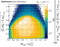
Refer to caption
Refer to caption
Refer to caption
Figure 31: Distributions of the sum of reconstructed W𝑊W mass estimators squared, (iMWi 2)/(imWi 2)subscript𝑖superscriptsubscript𝑀subscript𝑊𝑖2subscript𝑖superscriptsubscript𝑚subscript𝑊𝑖2\sqrt{(\sum_{i}M_{\footnotesize\mathrm{{\color[rgb]{0.45,0.0,0.09}\definecolor[named]{pgfstrokecolor}{rgb}{0.45,0.0,0.09}\textbf{$W_{i}$}}}}^{\footnotesize\leavevmode\nobreak\ 2})/(\sum_{i}m_{\footnotesize\mathrm{{\color[rgb]{0.45,0.0,0.09}\definecolor[named]{pgfstrokecolor}{rgb}{0.45,0.0,0.09}\textbf{$W_{i}$}}}}^{\footnotesize\leavevmode\nobreak\ 2})}, as a function of the estimated invariant mass of the total event, Mcmsuperscriptsubscript𝑀cmabsentM_{\footnotesize\mathrm{{\color[rgb]{0.45,0.0,0.09}\definecolor[named]{pgfstrokecolor}{rgb}{0.45,0.0,0.09}\textbf{cm}}}}^{\footnotesize\leavevmode\nobreak\ }, for simulated non-resonant N×W(ν)𝑁𝑊𝜈N\times W(\ell\nu) events. Both observables are normalized by the true values of the quantities they are estimating. Distributions are shown for (a) N=2𝑁2N=2, (b) N=3𝑁3N=3, and (c) N=4𝑁4N=4.

The lack of correlation between the W𝑊W boson mass and Mcmsuperscriptsubscript𝑀cmabsentM_{\footnotesize\mathrm{{\color[rgb]{0.45,0.0,0.09}\definecolor[named]{pgfstrokecolor}{rgb}{0.45,0.0,0.09}\textbf{cm}}}}^{\footnotesize\leavevmode\nobreak\ } estimators recalls Fig. 11 for HW+W𝐻superscript𝑊superscript𝑊H\rightarrow W^{+}W^{-} events, Fig. 15 for t~t~thadχ~10thadχ~10~𝑡~𝑡subscript𝑡hadsubscriptsuperscript~𝜒01subscript𝑡hadsubscriptsuperscript~𝜒01\tilde{t}\tilde{t}\rightarrow t_{\rm had}\tilde{\chi}^{0}_{1}t_{\rm had}\tilde{\chi}^{0}_{1}, and Fig. 17 for χ~20χ~20Z()χ~10h(γγ)χ~10superscriptsubscript~𝜒20superscriptsubscript~𝜒20𝑍subscriptsuperscript~𝜒01𝛾𝛾subscriptsuperscript~𝜒01\tilde{\chi}_{2}^{0}\tilde{\chi}_{2}^{0}\rightarrow Z(\ell\ell)\tilde{\chi}^{0}_{1}h(\gamma\gamma)\tilde{\chi}^{0}_{1}. The JR VIII.1 has recovers sensitivity to the mass of the W𝑊W’s, independently of Mcmsuperscriptsubscript𝑀cmabsentM_{\footnotesize\mathrm{{\color[rgb]{0.45,0.0,0.09}\definecolor[named]{pgfstrokecolor}{rgb}{0.45,0.0,0.09}\textbf{cm}}}}^{\footnotesize\leavevmode\nobreak\ }.

This JR is an important part of the RJR library, as it allows for the analysis of final states with an arbitrary number of invisible particles, with the quality of extracted information dependent on how well they can be paired with visible partners. While it is encouraging that useful information can still be measured in these highly non-resonant cases, additional structure in events can yield much more information, as we see in the following example.

VIII.2 HhhW(ν)W(ν)W(ν)W(ν)𝐻𝑊𝜈superscript𝑊𝜈𝑊𝜈superscript𝑊𝜈H\rightarrow hh\rightarrow W(\ell\nu)W^{*}(\ell\nu)W(\ell\nu)W^{*}(\ell\nu)

When analyzing events with many invisible particles in the final state, expected symmetries and relations between the intermediate particles possibly appearing in them can be used in the choice of JR’s. In this example, we consider the production of a heavy, neutral Higgs boson at a hadron collider, which decays to two, SM-like, Higgs bosons. Each of these lighter Higgs bosons then decays to two W𝑊W bosons which, in turn, decay to a lepton and neutrino. This leads to four leptons in the final state, V={a,a,a,b,b,a,b,b}Vsubscript𝑎𝑎subscript𝑎𝑏subscript𝑏𝑎subscript𝑏𝑏\mathrm{{\color[rgb]{0.1,0.1,0.44}\definecolor[named]{pgfstrokecolor}{rgb}{0.1,0.1,0.44}\textbf{V}}}=\{\mathrm{{\color[rgb]{0.1,0.1,0.44}\definecolor[named]{pgfstrokecolor}{rgb}{0.1,0.1,0.44}\textbf{$\ell_{a,a}$}}},\mathrm{{\color[rgb]{0.1,0.1,0.44}\definecolor[named]{pgfstrokecolor}{rgb}{0.1,0.1,0.44}\textbf{$\ell_{a,b}$}}},\mathrm{{\color[rgb]{0.1,0.1,0.44}\definecolor[named]{pgfstrokecolor}{rgb}{0.1,0.1,0.44}\textbf{$\ell_{b,a}$}}},\mathrm{{\color[rgb]{0.1,0.1,0.44}\definecolor[named]{pgfstrokecolor}{rgb}{0.1,0.1,0.44}\textbf{$\ell_{b,b}$}}}\}, and likely non-zero measured ETmisssuperscriptsubscript𝐸𝑇miss\vec{E}_{T}^{\rm miss}  associated with four escaping neutrinos, I={νa,a,νa,b,νb,a,νb,b}Isubscript𝜈𝑎𝑎subscript𝜈𝑎𝑏subscript𝜈𝑏𝑎subscript𝜈𝑏𝑏\mathrm{{\color[rgb]{0.12,0.3,0.17}\definecolor[named]{pgfstrokecolor}{rgb}{0.12,0.3,0.17}\textbf{I}}}=\{\mathrm{{\color[rgb]{0.12,0.3,0.17}\definecolor[named]{pgfstrokecolor}{rgb}{0.12,0.3,0.17}\textbf{$\nu_{a,a}$}}},\mathrm{{\color[rgb]{0.12,0.3,0.17}\definecolor[named]{pgfstrokecolor}{rgb}{0.12,0.3,0.17}\textbf{$\nu_{a,b}$}}},\mathrm{{\color[rgb]{0.12,0.3,0.17}\definecolor[named]{pgfstrokecolor}{rgb}{0.12,0.3,0.17}\textbf{$\nu_{b,a}$}}},\mathrm{{\color[rgb]{0.12,0.3,0.17}\definecolor[named]{pgfstrokecolor}{rgb}{0.12,0.3,0.17}\textbf{$\nu_{b,b}$}}}\}. The decay tree describing this final state is shown in Fig. 32.
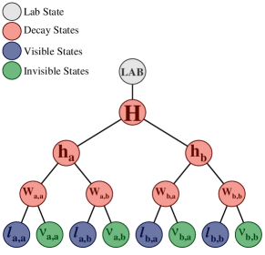
Refer to caption
Figure 32: A decay tree diagram for heavy, neutral Higgs production decaying to two lighter, neutral Higgs bosons. Each of the lighter Higgs’s is assumed to be SM-like and have a mass of mh=125superscriptsubscript𝑚absent125m_{\footnotesize\mathrm{{\color[rgb]{0.45,0.0,0.09}\definecolor[named]{pgfstrokecolor}{rgb}{0.45,0.0,0.09}\textbf{$h$}}}}^{\footnotesize\leavevmode\nobreak\ }=125 GeV, further decaying to W(ν)W(ν)𝑊𝜈superscript𝑊𝜈W(\ell\nu)W^{*}(\ell\nu). The heavy Higgs mass is chosen as mH=750superscriptsubscript𝑚𝐻absent750m_{\footnotesize\mathrm{{\color[rgb]{0.45,0.0,0.09}\definecolor[named]{pgfstrokecolor}{rgb}{0.45,0.0,0.09}\textbf{$H$}}}}^{\footnotesize\leavevmode\nobreak\ }=750 GeV. The final state has four visible leptons, with total charge zero.

As for the non-resonant 4W(ν)4𝑊𝜈4W(\ell\nu) example discussed in Section VIII.1, in order to reconstruct this event we must make choices for all the components of the neutrinos’ momentum that we are unable to measure directly. Applying the constraints pI,Tlab=ETmisssuperscriptsubscript𝑝I𝑇labsuperscriptsubscript𝐸𝑇miss\vec{p}_{\footnotesize\mathrm{{\color[rgb]{0.12,0.3,0.17}\definecolor[named]{pgfstrokecolor}{rgb}{0.12,0.3,0.17}\textbf{I}}},T}^{\footnotesize\leavevmode\nobreak\ \mathrm{\textbf{lab}}}=\vec{E}_{T}^{\rm miss} and Mνi=0superscriptsubscript𝑀subscript𝜈𝑖absent0M_{\footnotesize\mathrm{{\color[rgb]{0.12,0.3,0.17}\definecolor[named]{pgfstrokecolor}{rgb}{0.12,0.3,0.17}\textbf{$\nu_{i}$}}}}^{\footnotesize\leavevmode\nobreak\ }=0, there are still 10 under-constrained d.o.f. in each event. While the same JR VIII.1 can be used to resolve many of these unknowns simultaneously, in this case the expected symmetry between masses and decays of each lighter Higgs boson motivates a different strategy.

In the RJR approach we attempt to factorize the information we hope to extract about each decay step by considering it independently, choosing JR’s corresponding to its specific details, and desired constraints. For the decay of the heavy, neutral Higgs boson, H𝐻H, there are several pieces of information we must choose. Firstly, we assume that the total charge of the four leptons in the event is zero, such that there are two lepton/anti-lepton pairs, although not necessarily the same flavor. Defining the two opposite-sign pairs of leptons as Va={a,a,a,b}Vasubscript𝑎𝑎subscript𝑎𝑏\mathrm{{\color[rgb]{0.1,0.1,0.44}\definecolor[named]{pgfstrokecolor}{rgb}{0.1,0.1,0.44}\textbf{V${}_{a}$}}}=\{\mathrm{{\color[rgb]{0.1,0.1,0.44}\definecolor[named]{pgfstrokecolor}{rgb}{0.1,0.1,0.44}\textbf{$\ell_{a,a}$}}},\mathrm{{\color[rgb]{0.1,0.1,0.44}\definecolor[named]{pgfstrokecolor}{rgb}{0.1,0.1,0.44}\textbf{$\ell_{a,b}$}}}\} and Vb={b,a,b,b}Vbsubscript𝑏𝑎subscript𝑏𝑏\mathrm{{\color[rgb]{0.1,0.1,0.44}\definecolor[named]{pgfstrokecolor}{rgb}{0.1,0.1,0.44}\textbf{V${}_{b}$}}}=\{\mathrm{{\color[rgb]{0.1,0.1,0.44}\definecolor[named]{pgfstrokecolor}{rgb}{0.1,0.1,0.44}\textbf{$\ell_{b,a}$}}},\mathrm{{\color[rgb]{0.1,0.1,0.44}\definecolor[named]{pgfstrokecolor}{rgb}{0.1,0.1,0.44}\textbf{$\ell_{b,b}$}}}\}, we choose the assignment which minimizes the quantity mVa 2+mVb 2superscriptsubscript𝑚Va2superscriptsubscript𝑚Vb2m_{\footnotesize\mathrm{{\color[rgb]{0.1,0.1,0.44}\definecolor[named]{pgfstrokecolor}{rgb}{0.1,0.1,0.44}\textbf{V${}_{a}$}}}}^{\footnotesize\leavevmode\nobreak\ 2}+m_{\footnotesize\mathrm{{\color[rgb]{0.1,0.1,0.44}\definecolor[named]{pgfstrokecolor}{rgb}{0.1,0.1,0.44}\textbf{V${}_{b}$}}}}^{\footnotesize\leavevmode\nobreak\ 2}, according to JR VII.1.1.

When choosing the unknowns describing how the four neutrino system kinematically splits into two pairs in this decay, the expected similarity between the two SM-like Higgs masses can be exploited in the context of a contra-boost invariant JR VI.4, imposing the constraint Mha=Mhbsuperscriptsubscript𝑀subscript𝑎absentsuperscriptsubscript𝑀subscript𝑏absentM_{\footnotesize\mathrm{{\color[rgb]{0.45,0.0,0.09}\definecolor[named]{pgfstrokecolor}{rgb}{0.45,0.0,0.09}\textbf{$h_{a}$}}}}^{\footnotesize\leavevmode\nobreak\ }=M_{\footnotesize\mathrm{{\color[rgb]{0.45,0.0,0.09}\definecolor[named]{pgfstrokecolor}{rgb}{0.45,0.0,0.09}\textbf{$h_{b}$}}}}^{\footnotesize\leavevmode\nobreak\ }. The application of this JR only describes the momentum of the two neutrino pairs in the approximation of the H𝐻H rest frame, and uses only information about the total momentum of the pairs Va and Vb, without resolving that they are each made up of two separate particles. This is a crucial distinction, in that it ensures that the estimators describing each decay are maximally uncorrelated, as they are largely based on different information.

As explained in Section VI.3, the use of the contra-boost invariant JR VI.4 imposes specific constraints on the estimated masses of the individual invisible particles after the pair is split, in this case the two systems of neutrino pairs, Ia={νa,a,νa,b}Iasubscript𝜈𝑎𝑎subscript𝜈𝑎𝑏\mathrm{{\color[rgb]{0.12,0.3,0.17}\definecolor[named]{pgfstrokecolor}{rgb}{0.12,0.3,0.17}\textbf{I${}_{a}$}}}=\{\mathrm{{\color[rgb]{0.12,0.3,0.17}\definecolor[named]{pgfstrokecolor}{rgb}{0.12,0.3,0.17}\textbf{$\nu_{a,a}$}}},\mathrm{{\color[rgb]{0.12,0.3,0.17}\definecolor[named]{pgfstrokecolor}{rgb}{0.12,0.3,0.17}\textbf{$\nu_{a,b}$}}}\} and Ib={νb,a,νb,b}Ibsubscript𝜈𝑏𝑎subscript𝜈𝑏𝑏\mathrm{{\color[rgb]{0.12,0.3,0.17}\definecolor[named]{pgfstrokecolor}{rgb}{0.12,0.3,0.17}\textbf{I${}_{b}$}}}=\{\mathrm{{\color[rgb]{0.12,0.3,0.17}\definecolor[named]{pgfstrokecolor}{rgb}{0.12,0.3,0.17}\textbf{$\nu_{b,a}$}}},\mathrm{{\color[rgb]{0.12,0.3,0.17}\definecolor[named]{pgfstrokecolor}{rgb}{0.12,0.3,0.17}\textbf{$\nu_{b,b}$}}}\}. As the JR forces the two Higgs masses to be equal, any difference between the masses of the two lepton pairs will result in a difference between MIasuperscriptsubscript𝑀IaabsentM_{\footnotesize\mathrm{{\color[rgb]{0.12,0.3,0.17}\definecolor[named]{pgfstrokecolor}{rgb}{0.12,0.3,0.17}\textbf{I${}_{a}$}}}}^{\footnotesize\leavevmode\nobreak\ } and MIbsuperscriptsubscript𝑀IbabsentM_{\footnotesize\mathrm{{\color[rgb]{0.12,0.3,0.17}\definecolor[named]{pgfstrokecolor}{rgb}{0.12,0.3,0.17}\textbf{I${}_{b}$}}}}^{\footnotesize\leavevmode\nobreak\ }. Since the lepton pairs are coming from the same decays as the neutrinos, the lepton pair masses are good indicators of the corresponding neutrino masses. To prevent any biases in the kinematics of the neutrino system from being introduced by the JR, we choose MIa=2|pb,a/bVb|MVbsuperscriptsubscript𝑀Iaabsent2superscriptsubscript𝑝subscript𝑏𝑎𝑏Vbsuperscriptsubscript𝑀VbabsentM_{\footnotesize\mathrm{{\color[rgb]{0.12,0.3,0.17}\definecolor[named]{pgfstrokecolor}{rgb}{0.12,0.3,0.17}\textbf{I${}_{a}$}}}}^{\footnotesize\leavevmode\nobreak\ }=2|\vec{p}_{\footnotesize\mathrm{{\color[rgb]{0.1,0.1,0.44}\definecolor[named]{pgfstrokecolor}{rgb}{0.1,0.1,0.44}\textbf{$\ell_{b,a/b}$}}}}^{\footnotesize\leavevmode\nobreak\ \mathrm{{\color[rgb]{0.1,0.1,0.44}\definecolor[named]{pgfstrokecolor}{rgb}{0.1,0.1,0.44}\textbf{V${}_{b}$}}}}|\approx M_{\footnotesize\mathrm{{\color[rgb]{0.1,0.1,0.44}\definecolor[named]{pgfstrokecolor}{rgb}{0.1,0.1,0.44}\textbf{V${}_{b}$}}}}^{\footnotesize\leavevmode\nobreak\ } and MIb=2|pa,a/bVa|superscriptsubscript𝑀Ibabsent2superscriptsubscript𝑝subscript𝑎𝑎𝑏VaM_{\footnotesize\mathrm{{\color[rgb]{0.12,0.3,0.17}\definecolor[named]{pgfstrokecolor}{rgb}{0.12,0.3,0.17}\textbf{I${}_{b}$}}}}^{\footnotesize\leavevmode\nobreak\ }=2|\vec{p}_{\footnotesize\mathrm{{\color[rgb]{0.1,0.1,0.44}\definecolor[named]{pgfstrokecolor}{rgb}{0.1,0.1,0.44}\textbf{$\ell_{a,a/b}$}}}}^{\footnotesize\leavevmode\nobreak\ \mathrm{{\color[rgb]{0.1,0.1,0.44}\definecolor[named]{pgfstrokecolor}{rgb}{0.1,0.1,0.44}\textbf{V${}_{a}$}}}}|. This corresponds to a choice MI=mVsuperscriptsubscript𝑀Iabsentsuperscriptsubscript𝑚VabsentM_{\footnotesize\mathrm{{\color[rgb]{0.12,0.3,0.17}\definecolor[named]{pgfstrokecolor}{rgb}{0.12,0.3,0.17}\textbf{I}}}}^{\footnotesize\leavevmode\nobreak\ }=m_{\footnotesize\mathrm{{\color[rgb]{0.1,0.1,0.44}\definecolor[named]{pgfstrokecolor}{rgb}{0.1,0.1,0.44}\textbf{V}}}}^{\footnotesize\leavevmode\nobreak\ }.

In the subsequent decays of the Higgs bosons, hasubscript𝑎h_{a} and hbsubscript𝑏h_{b}, the same decay topology is encountered, with visible and invisible particle pairs splitting in two. As mh2mWsuperscriptsubscript𝑚absent2superscriptsubscript𝑚𝑊absentm_{\footnotesize\mathrm{{\color[rgb]{0.45,0.0,0.09}\definecolor[named]{pgfstrokecolor}{rgb}{0.45,0.0,0.09}\textbf{$h$}}}}^{\footnotesize\leavevmode\nobreak\ }\leq 2m_{\footnotesize\mathrm{{\color[rgb]{0.45,0.0,0.09}\definecolor[named]{pgfstrokecolor}{rgb}{0.45,0.0,0.09}\textbf{$W$}}}}^{\footnotesize\leavevmode\nobreak\ }, one of the W𝑊W bosons is generally produced off-shell in each decay, meaning that constraining the two W𝑊W masses in these decays to be equal would be inaccurate. Instead, a more generic jigsaw minimizing the sum of W𝑊W masses in each decay, JR VIII.1, is used, allowing the individual neutrino mass estimators to be fixed to zero.

With these choices of JR’s, the strategy for analyzing HhhW(ν)W(ν)W(ν)W(ν)𝐻𝑊𝜈superscript𝑊𝜈𝑊𝜈superscript𝑊𝜈H\rightarrow hh\rightarrow W(\ell\nu)W^{*}(\ell\nu)W(\ell\nu)W^{*}(\ell\nu) events at a hadron collider can be summarized as:

  1. 1.

    Apply the combinatoric JR VII.1.1, choosing the lepton pairing that minimizes mVa 2+mVb 2superscriptsubscript𝑚Va2superscriptsubscript𝑚Vb2m_{\footnotesize\mathrm{{\color[rgb]{0.1,0.1,0.44}\definecolor[named]{pgfstrokecolor}{rgb}{0.1,0.1,0.44}\textbf{V${}_{a}$}}}}^{\footnotesize\leavevmode\nobreak\ 2}+m_{\footnotesize\mathrm{{\color[rgb]{0.1,0.1,0.44}\definecolor[named]{pgfstrokecolor}{rgb}{0.1,0.1,0.44}\textbf{V${}_{b}$}}}}^{\footnotesize\leavevmode\nobreak\ 2}.

  2. 2.

    Apply the invisible mass JR VI.1,
    choosing MI=mVsuperscriptsubscript𝑀Iabsentsuperscriptsubscript𝑚VabsentM_{\footnotesize\mathrm{{\color[rgb]{0.12,0.3,0.17}\definecolor[named]{pgfstrokecolor}{rgb}{0.12,0.3,0.17}\textbf{I}}}}^{\footnotesize\leavevmode\nobreak\ }=m_{\footnotesize\mathrm{{\color[rgb]{0.1,0.1,0.44}\definecolor[named]{pgfstrokecolor}{rgb}{0.1,0.1,0.44}\textbf{V}}}}^{\footnotesize\leavevmode\nobreak\ }.

  3. 3.

    Apply the invisible rapidity JR V.1, choosing
    pI,zlabsuperscriptsubscript𝑝I𝑧labp_{\footnotesize\mathrm{{\color[rgb]{0.12,0.3,0.17}\definecolor[named]{pgfstrokecolor}{rgb}{0.12,0.3,0.17}\textbf{I}}},z}^{\footnotesize\leavevmode\nobreak\ \mathrm{\textbf{lab}}} using the collection of leptons, V.

  4. 4.

    Apply the contra-boost invariant JR VI.4, using
    the constraint Mha=Mhbsuperscriptsubscript𝑀subscript𝑎absentsuperscriptsubscript𝑀subscript𝑏absentM_{\footnotesize\mathrm{{\color[rgb]{0.45,0.0,0.09}\definecolor[named]{pgfstrokecolor}{rgb}{0.45,0.0,0.09}\textbf{$h_{a}$}}}}^{\footnotesize\leavevmode\nobreak\ }=M_{\footnotesize\mathrm{{\color[rgb]{0.45,0.0,0.09}\definecolor[named]{pgfstrokecolor}{rgb}{0.45,0.0,0.09}\textbf{$h_{b}$}}}}^{\footnotesize\leavevmode\nobreak\ }.

  5. 5.

    Apply the JR VIII.1 for each ha/bsubscript𝑎𝑏h_{a/b} decay,
    minimizing MWa/b,a 2+MWa/b,b 2superscriptsubscript𝑀subscript𝑊𝑎𝑏𝑎2superscriptsubscript𝑀subscript𝑊𝑎𝑏𝑏2M_{\footnotesize\mathrm{{\color[rgb]{0.45,0.0,0.09}\definecolor[named]{pgfstrokecolor}{rgb}{0.45,0.0,0.09}\textbf{$W_{a/b,a}$}}}}^{\footnotesize\leavevmode\nobreak\ 2}+M_{\footnotesize\mathrm{{\color[rgb]{0.45,0.0,0.09}\definecolor[named]{pgfstrokecolor}{rgb}{0.45,0.0,0.09}\textbf{$W_{a/b,b}$}}}}^{\footnotesize\leavevmode\nobreak\ 2}.

In the context of searching for evidence of this phenomenon, the masses and decay angles of the three Higgs bosons are of primary interest. Even though the two SM-like Higgs masses have been constrained to be the same by the contra-boost invariant JR, we can recover independent information about them by using alternative quantities as estimators. The Higgs mass equality required that we set the di-neutrino pair masses equal to that of the di-leptons of the opposite half of the event, a guess that was made for the convenience of the JR. To make the effective mass estimators more independent of this choice, we instead adopt the convention: Mha/b=2EVa/bha/bsubscript𝑀subscript𝑎𝑏2superscriptsubscript𝐸Va/bsubscript𝑎𝑏M_{h_{a/b}}=2E_{\footnotesize\mathrm{{\color[rgb]{0.1,0.1,0.44}\definecolor[named]{pgfstrokecolor}{rgb}{0.1,0.1,0.44}\textbf{V${}_{a/b}$}}}}^{\footnotesize\leavevmode\nobreak\ \mathrm{{\color[rgb]{0.45,0.0,0.09}\definecolor[named]{pgfstrokecolor}{rgb}{0.45,0.0,0.09}\textbf{$h_{a/b}$}}}}, where this equivalence is used only for purposes of data-analysis, and does not change the reconstruction of the event.

The distributions of the mass estimators and reconstructed decay angles of the three Higgs bosons are shown in Fig. 33 for simulated events with mH=750superscriptsubscript𝑚𝐻absent750m_{\footnotesize\mathrm{{\color[rgb]{0.45,0.0,0.09}\definecolor[named]{pgfstrokecolor}{rgb}{0.45,0.0,0.09}\textbf{$H$}}}}^{\footnotesize\leavevmode\nobreak\ }=750 GeV. The SM-like Higgs masses are almost completely uncorrelated, with both masses showing a slight downward bias relative to the true value and a resolution of 20%similar-toabsentpercent20\sim 20\%. Here, the choice of estimators is contradictory to the reconstructed interpretation of the event resulting from the application of JR’s, a strategy which is discussed in more detail in the following example.

The SM-like Higgs mass observables are also independent of the heavy Higgs mass, as seen in Fig. 33(b), demonstrating that all three masses can be extracted separately, with similar resolution. Similarly, each of the Higgs’ reconstructed decay angles can be estimated with excellent precision, independently of each other, with not even small correlations observed in their distributions, as seen in Fig. 33(d,e).

There is even more information contained in the approximations of the W𝑊W rest frames, including masses and decay angles, as can be seen in the distributions of these quantities for the on-shell W𝑊W in Fig. 33(c,f). As was the case for the SM-like Higgs decays, these estimators are almost completely uncorrelated with the previous ones, with the distribution of the W𝑊W mass estimator exhibiting a kinematic edge at the true value, almost identically to W(ν)𝑊𝜈W(\ell\nu) pair production in Fig. 31 from the previous example. The observables from each decay step behave as if that was the entire decay tree, with little sensitivity to the details of other decays in the event. As additional decays are added, the resolution of some observables degrade, but the accuracy of estimators further up the decay tree improve, as integrating over more degrees of freedom in the event further smooths the kinematics and the applied approximations become better.

While the ability to accurately measure these quantities is important for studying this type of process, it is equally useful when searching for evidence of it, as SM backgrounds in this final state would have to mimic the targeted process independently in many observable dimensions. The recursive application of JR’s at each step in the decay, effectively analyzing each reference frame independently of the others, can be used to derive an appropriate basis of observables for either purpose.
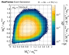
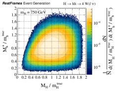
Refer to caption
Refer to caption
Refer to caption
Refer to caption
Refer to caption
Refer to caption
Figure 33: Distributions of (a) one SM Higgs mass estimator, as a function of the other, and (b) one SM Higgs mass estimator, as a function of the heavy Higgs mass, (c) the on-shell W𝑊W mass estimator, max(MWa,a,MWa,b)superscriptsubscript𝑀subscript𝑊𝑎𝑎absentsuperscriptsubscript𝑀subscript𝑊𝑎𝑏absent\max(M_{\footnotesize\mathrm{{\color[rgb]{0.45,0.0,0.09}\definecolor[named]{pgfstrokecolor}{rgb}{0.45,0.0,0.09}\textbf{$W_{a,a}$}}}}^{\footnotesize\leavevmode\nobreak\ },M_{\footnotesize\mathrm{{\color[rgb]{0.45,0.0,0.09}\definecolor[named]{pgfstrokecolor}{rgb}{0.45,0.0,0.09}\textbf{$W_{a,b}$}}}}^{\footnotesize\leavevmode\nobreak\ }), as a function of its associated Higgs mass, (d) the reconstructed decay angle of one SM Higgs boson, as a function of the other, and (e) one SM Higgs boson decay angle, as a function of the reconstructed heavy Higgs decay angle, and (f) the on-shell W𝑊W decay angle, as a function of the corresponding SM Higgs boson decay angle, for simulated Hhh4W(ν)𝐻4𝑊𝜈H\rightarrow hh\rightarrow 4W(\ell\nu) events. Each observable is normalized appropriately by the true value of the quantity it is estimating, with angles expressed in units radian.

VIII.3 g~g~bbχ~10bbχ~10~𝑔~𝑔𝑏𝑏subscriptsuperscript~𝜒01𝑏𝑏subscriptsuperscript~𝜒01\tilde{g}\tilde{g}\rightarrow bb\tilde{\chi}^{0}_{1}bb\tilde{\chi}^{0}_{1} at a hadron collider

All the previous examples have primarily focused on JR’s for resolving the kinematics of invisible particles, with a variety of choices for nearly every decay possibility. In order to be able to analyze every imaginable decay topology with the RJR approach, additional treatments for combinatoric ambiguities, resulting from indistinguishable reconstructed particles appearing in events, are introduced.

Like the invisible JR VIII.1 which minimizes the masses squared of potentially many composite particles simultaneously, the combinatoric analogue JR VII.1.1 can be generalized to an arbitrarily large number of particles and partitions. But simultaneously choosing many unknowns in a single decay step, rather than factorizing the unknowns into several steps, results in a degradation in resolution of kinematic estimators, as seen in the comparison of analysis strategies for 4W(ν)4𝑊𝜈4W(\ell\nu) final states between Sections VIII.1 and VIII.2. Just as for invisible particle JR’s, using combinatoric jigsaws in recursive steps can help resolve intermediate structure in decays.

To demonstrate this idea, we consider the example of gluino and sbottom quark production at a hadron collider, with decays to b𝑏b-quarks and neutralinos. While different b𝑏b-quarks may appear in different places in a decay tree, the reconstructed b𝑏b-tagged jets are indistinguishable, with no direct indication which one is which. We consider four different combinations of gluino and sbottom production and decay, with the processes summarized in Fig. 34. The sbottom quarks in these events each decay to a b𝑏b-quark and a neutralino, while two different gluino decays are considered. When the gluino is heavier than the sbottom, it can decay g~bb~~𝑔𝑏~𝑏\tilde{g}\rightarrow b\tilde{b}, resulting in two b𝑏b-quarks and a neutralino after the sbottom quarks decay. Alternatively, if the squarks are much heavier than the gluino, it can undergo a three-body decay through a virtual sbottom quark to the same final state. The production and decays illustrated in Fig. 34(d) contain two gluinos, each decaying in a different way. While kinematically disfavored, this process is included to demonstrate the independent sensitivity of the reconstruction scheme to the two separate decays.

All of the processes appearing in Fig. 34 can be analyzed with a single decay tree, shown in Fig. 35. The objects P~a/bsubscript~𝑃𝑎𝑏\tilde{P}_{a/b} represent the initially produced sparticles, either sbottom quarks or gluinos, while the C~a/bsubscript~𝐶𝑎𝑏\tilde{C}_{a/b} are any additional sparticles which might appear in the decays. Neutralinos are represented by the invisible states Ia/b, with the reconstructed b𝑏b-tagged jets corresponding to the visible states Vij. While the largest number of b𝑏b-tagged jets in the final state is four in the processes explicitly considered in this example, the reconstruction approach adopted here allows for an arbitrarily high number. If, instead, the sbottoms in this example were squarks associated with the light quarks, the visible jets in the final state would be initiated by quarks and gluons, and indistinguishable from any other jets from the underlying event or mis-identified pile-up interactions. To account for larger multiplicities of identical visible particles in the final state, each Vij is interpreted as a set of b𝑏b-tagged jets that can contain a variable number, subject to defined constraints. We require that each V2a/b contain at least one element in each event, while V1a/b are permitted to have none.
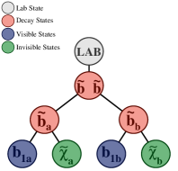
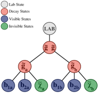
Refer to caption
Refer to caption
Refer to caption
Refer to caption
Figure 34: Decay tree diagrams for the pair production of strongly interacting sparticles decaying to final states with b𝑏b-quarks and neutralinos. (a) Two sbottom quarks are produced, each decaying to a b𝑏b-quark and neutralino. (b) Pair produced gluinos each undergo a three-body decay to two b𝑏b-quarks and a neutralino. (c) Two gluinos are produced, each decaying to a b𝑏b-quark and a sbottom quark which, in turn, decays to a b𝑏b-quark and a neutralino. (d) Pair produced gluinos each decay in a different way, one corresponding to the decays in (b), the other the decays in (c). In each of these four scenarios, the mass of the initially produced parent sparticles is 1 TeV, while mχ~10=100superscriptsubscript𝑚subscriptsuperscript~𝜒01absent100m_{\footnotesize\mathrm{{\color[rgb]{0.12,0.3,0.17}\definecolor[named]{pgfstrokecolor}{rgb}{0.12,0.3,0.17}\textbf{$\tilde{\chi}^{0}_{1}$}}}}^{\footnotesize\leavevmode\nobreak\ }=100 GeV. When appearing in the decays of gluinos, sbottoms are chosen to have a mass of mb~=900superscriptsubscript𝑚~𝑏absent900m_{\footnotesize\mathrm{{\color[rgb]{0.45,0.0,0.09}\definecolor[named]{pgfstrokecolor}{rgb}{0.45,0.0,0.09}\textbf{$\tilde{b}$}}}}^{\footnotesize\leavevmode\nobreak\ }=900 GeV in this example.
Refer to caption
Figure 35: Decay tree for analyzing strong sparticle pair production, with the decays described in Fig. 34. The intermediate decay states, P~isubscript~𝑃𝑖\tilde{P}_{i} and C~isubscript~𝐶𝑖\tilde{C}_{i}, represent the sparticles that may appear in the event, while the visible states, Vij, represent a set of b𝑏b-tagged jets.

Defining V={bi}Vsubscript𝑏𝑖\mathrm{{\color[rgb]{0.1,0.1,0.44}\definecolor[named]{pgfstrokecolor}{rgb}{0.1,0.1,0.44}\textbf{V}}}=\{\mathrm{{\color[rgb]{0.1,0.1,0.44}\definecolor[named]{pgfstrokecolor}{rgb}{0.1,0.1,0.44}\textbf{$b_{i}$}}}\} to be the set of all b𝑏b-tagged jets reconstructed in the event, the combinatoric unknowns are those associated with partitioning this set into these four subsets. Matching the decay tree in Fig. 35, the partitioning is done in two steps with separate JR’s, the first splitting V into two sets, Va={V1a,V2a}VaV1aV2a\mathrm{{\color[rgb]{0.1,0.1,0.44}\definecolor[named]{pgfstrokecolor}{rgb}{0.1,0.1,0.44}\textbf{V${}_{a}$}}}=\{\mathrm{{\color[rgb]{0.1,0.1,0.44}\definecolor[named]{pgfstrokecolor}{rgb}{0.1,0.1,0.44}\textbf{V${}_{1a}$}}},\mathrm{{\color[rgb]{0.1,0.1,0.44}\definecolor[named]{pgfstrokecolor}{rgb}{0.1,0.1,0.44}\textbf{V${}_{2a}$}}}\} and Vb={V1b,V2b}VbV1bV2b\mathrm{{\color[rgb]{0.1,0.1,0.44}\definecolor[named]{pgfstrokecolor}{rgb}{0.1,0.1,0.44}\textbf{V${}_{b}$}}}=\{\mathrm{{\color[rgb]{0.1,0.1,0.44}\definecolor[named]{pgfstrokecolor}{rgb}{0.1,0.1,0.44}\textbf{V${}_{1b}$}}},\mathrm{{\color[rgb]{0.1,0.1,0.44}\definecolor[named]{pgfstrokecolor}{rgb}{0.1,0.1,0.44}\textbf{V${}_{2b}$}}}\}. While the combinatoric JR VII.1.1, which chooses this partition by minimizing the combination mVa 2+mVb 2superscriptsubscript𝑚Va2superscriptsubscript𝑚Vb2m_{\footnotesize\mathrm{{\color[rgb]{0.1,0.1,0.44}\definecolor[named]{pgfstrokecolor}{rgb}{0.1,0.1,0.44}\textbf{V${}_{a}$}}}}^{\footnotesize\leavevmode\nobreak\ 2}+m_{\footnotesize\mathrm{{\color[rgb]{0.1,0.1,0.44}\definecolor[named]{pgfstrokecolor}{rgb}{0.1,0.1,0.44}\textbf{V${}_{b}$}}}}^{\footnotesize\leavevmode\nobreak\ 2}, can be used, there is a practical limitation in cases where nV=|V|subscript𝑛VVn_{\mathrm{{\color[rgb]{0.1,0.1,0.44}\definecolor[named]{pgfstrokecolor}{rgb}{0.1,0.1,0.44}\textbf{V}}}}=|\mathrm{{\color[rgb]{0.1,0.1,0.44}\definecolor[named]{pgfstrokecolor}{rgb}{0.1,0.1,0.44}\textbf{V}}}| is large. Asymptotically, this algorithm scales as 2nV1nVlognVsuperscript2subscript𝑛V1subscript𝑛Vsubscript𝑛V2^{n_{\mathrm{{\color[rgb]{0.1,0.1,0.44}\definecolor[named]{pgfstrokecolor}{rgb}{0.1,0.1,0.44}\textbf{V}}}}-1}n_{\mathrm{{\color[rgb]{0.1,0.1,0.44}\definecolor[named]{pgfstrokecolor}{rgb}{0.1,0.1,0.44}\textbf{V}}}}\log n_{\mathrm{{\color[rgb]{0.1,0.1,0.44}\definecolor[named]{pgfstrokecolor}{rgb}{0.1,0.1,0.44}\textbf{V}}}}, which is computationally taxing. When computational time is limited, it is potentially prohibitive. To overcome this shortcoming, we introduce an additional combinatoric JR for partitioning a set into two groups which scales as nV3superscriptsubscript𝑛V3n_{\mathrm{{\color[rgb]{0.1,0.1,0.44}\definecolor[named]{pgfstrokecolor}{rgb}{0.1,0.1,0.44}\textbf{V}}}}^{3}, with a natural choice of minimized metric. The JR can be defined as follows Jackson:2016mfb :

Jigsaw Rule VIII.2 (Combinatoric Minimization)

If there is a set of n2𝑛2n\geq 2 visible particles, V={V1,,Vn}VV1Vn\mathrm{{\color[rgb]{0.1,0.1,0.44}\definecolor[named]{pgfstrokecolor}{rgb}{0.1,0.1,0.44}\textbf{V}}}=\{\mathrm{{\color[rgb]{0.1,0.1,0.44}\definecolor[named]{pgfstrokecolor}{rgb}{0.1,0.1,0.44}\textbf{V${}_{1}$}}},\cdots,\mathrm{{\color[rgb]{0.1,0.1,0.44}\definecolor[named]{pgfstrokecolor}{rgb}{0.1,0.1,0.44}\textbf{V${}_{n}$}}}\}, we can choose a partition of V into two subsets, PV={SVa,SVb}subscript𝑃Vsubscript𝑆Vasubscript𝑆VbP_{\mathrm{{\color[rgb]{0.1,0.1,0.44}\definecolor[named]{pgfstrokecolor}{rgb}{0.1,0.1,0.44}\textbf{V}}}}=\{S_{\mathrm{{\color[rgb]{0.1,0.1,0.44}\definecolor[named]{pgfstrokecolor}{rgb}{0.1,0.1,0.44}\textbf{V$a$}}}},S_{\mathrm{{\color[rgb]{0.1,0.1,0.44}\definecolor[named]{pgfstrokecolor}{rgb}{0.1,0.1,0.44}\textbf{V$b$}}}}\} by effectively minimizing the masses of the two subsets over the space of all valid partitions PVVsubscript𝑃VsubscriptVP_{\mathrm{{\color[rgb]{0.1,0.1,0.44}\definecolor[named]{pgfstrokecolor}{rgb}{0.1,0.1,0.44}\textbf{V}}}}\in\mathbb{P}_{\mathrm{{\color[rgb]{0.1,0.1,0.44}\definecolor[named]{pgfstrokecolor}{rgb}{0.1,0.1,0.44}\textbf{V}}}}. This rule is applicable when the only requirement on SVasubscript𝑆VaS_{\mathrm{{\color[rgb]{0.1,0.1,0.44}\definecolor[named]{pgfstrokecolor}{rgb}{0.1,0.1,0.44}\textbf{V$a$}}}} and SVbsubscript𝑆VbS_{\mathrm{{\color[rgb]{0.1,0.1,0.44}\definecolor[named]{pgfstrokecolor}{rgb}{0.1,0.1,0.44}\textbf{V$b$}}}} is that they each contain at least one element.

The partition is chosen by evaluating the four vectors of the visible particles in their mutual center-of-mass frame, and noting that pSVaV=pSVbVsuperscriptsubscript𝑝subscript𝑆VaVsuperscriptsubscript𝑝subscript𝑆VbV\vec{p}_{\footnotesize S_{\mathrm{{\color[rgb]{0.1,0.1,0.44}\definecolor[named]{pgfstrokecolor}{rgb}{0.1,0.1,0.44}\textbf{V$a$}}}}}^{\footnotesize\leavevmode\nobreak\ \mathrm{{\color[rgb]{0.1,0.1,0.44}\definecolor[named]{pgfstrokecolor}{rgb}{0.1,0.1,0.44}\textbf{V}}}}=-\vec{p}_{\footnotesize S_{\mathrm{{\color[rgb]{0.1,0.1,0.44}\definecolor[named]{pgfstrokecolor}{rgb}{0.1,0.1,0.44}\textbf{V$b$}}}}}^{\footnotesize\leavevmode\nobreak\ \mathrm{{\color[rgb]{0.1,0.1,0.44}\definecolor[named]{pgfstrokecolor}{rgb}{0.1,0.1,0.44}\textbf{V}}}}, irrespective of chosen partition. As mVsuperscriptsubscript𝑚Vabsentm_{\footnotesize\mathrm{{\color[rgb]{0.1,0.1,0.44}\definecolor[named]{pgfstrokecolor}{rgb}{0.1,0.1,0.44}\textbf{V}}}}^{\footnotesize\leavevmode\nobreak\ } is also independent of PVsubscript𝑃VP_{\mathrm{{\color[rgb]{0.1,0.1,0.44}\definecolor[named]{pgfstrokecolor}{rgb}{0.1,0.1,0.44}\textbf{V}}}}, the relation

mV=|pSVa/bV|2+mVa 2+|pSVa/bV|2+mVb 2,superscriptsubscript𝑚Vabsentsuperscriptsuperscriptsubscript𝑝subscript𝑆Va/bV2superscriptsubscript𝑚Va2superscriptsuperscriptsubscript𝑝subscript𝑆Va/bV2superscriptsubscript𝑚Vb2\displaystyle m_{\footnotesize\mathrm{{\color[rgb]{0.1,0.1,0.44}\definecolor[named]{pgfstrokecolor}{rgb}{0.1,0.1,0.44}\textbf{V}}}}^{\footnotesize\leavevmode\nobreak\ }=\sqrt{|\vec{p}_{\footnotesize S_{\mathrm{{\color[rgb]{0.1,0.1,0.44}\definecolor[named]{pgfstrokecolor}{rgb}{0.1,0.1,0.44}\textbf{V$a/b$}}}}}^{\footnotesize\leavevmode\nobreak\ \mathrm{{\color[rgb]{0.1,0.1,0.44}\definecolor[named]{pgfstrokecolor}{rgb}{0.1,0.1,0.44}\textbf{V}}}}|^{2}+m_{\footnotesize\mathrm{{\color[rgb]{0.1,0.1,0.44}\definecolor[named]{pgfstrokecolor}{rgb}{0.1,0.1,0.44}\textbf{V${}_{a}$}}}}^{\footnotesize\leavevmode\nobreak\ 2}}+\sqrt{|\vec{p}_{\footnotesize S_{\mathrm{{\color[rgb]{0.1,0.1,0.44}\definecolor[named]{pgfstrokecolor}{rgb}{0.1,0.1,0.44}\textbf{V$a/b$}}}}}^{\footnotesize\leavevmode\nobreak\ \mathrm{{\color[rgb]{0.1,0.1,0.44}\definecolor[named]{pgfstrokecolor}{rgb}{0.1,0.1,0.44}\textbf{V}}}}|^{2}+m_{\footnotesize\mathrm{{\color[rgb]{0.1,0.1,0.44}\definecolor[named]{pgfstrokecolor}{rgb}{0.1,0.1,0.44}\textbf{V${}_{b}$}}}}^{\footnotesize\leavevmode\nobreak\ 2}}\leavevmode\nobreak\ , (73)

implies that maximizing the momentum |pSVa/bV|superscriptsubscript𝑝subscript𝑆Va/bV|\vec{p}_{\footnotesize S_{\mathrm{{\color[rgb]{0.1,0.1,0.44}\definecolor[named]{pgfstrokecolor}{rgb}{0.1,0.1,0.44}\textbf{V$a/b$}}}}}^{\footnotesize\leavevmode\nobreak\ \mathrm{{\color[rgb]{0.1,0.1,0.44}\definecolor[named]{pgfstrokecolor}{rgb}{0.1,0.1,0.44}\textbf{V}}}}| is equivalent to simultaneously minimizing mVasuperscriptsubscript𝑚Vaabsentm_{\footnotesize\mathrm{{\color[rgb]{0.1,0.1,0.44}\definecolor[named]{pgfstrokecolor}{rgb}{0.1,0.1,0.44}\textbf{V${}_{a}$}}}}^{\footnotesize\leavevmode\nobreak\ } and mVbsuperscriptsubscript𝑚Vbabsentm_{\footnotesize\mathrm{{\color[rgb]{0.1,0.1,0.44}\definecolor[named]{pgfstrokecolor}{rgb}{0.1,0.1,0.44}\textbf{V${}_{b}$}}}}^{\footnotesize\leavevmode\nobreak\ }. This is accomplished by choosing PVsubscript𝑃VP_{\mathrm{{\color[rgb]{0.1,0.1,0.44}\definecolor[named]{pgfstrokecolor}{rgb}{0.1,0.1,0.44}\textbf{V}}}} which maximizes the function:

f(PV)=|pSVaV|+|pSVbV|,𝑓subscript𝑃Vsuperscriptsubscript𝑝subscript𝑆VaVsuperscriptsubscript𝑝subscript𝑆VbV\displaystyle f(P_{\mathrm{{\color[rgb]{0.1,0.1,0.44}\definecolor[named]{pgfstrokecolor}{rgb}{0.1,0.1,0.44}\textbf{V}}}})=|\vec{p}_{\footnotesize S_{\mathrm{{\color[rgb]{0.1,0.1,0.44}\definecolor[named]{pgfstrokecolor}{rgb}{0.1,0.1,0.44}\textbf{V$a$}}}}}^{\footnotesize\leavevmode\nobreak\ \mathrm{{\color[rgb]{0.1,0.1,0.44}\definecolor[named]{pgfstrokecolor}{rgb}{0.1,0.1,0.44}\textbf{V}}}}|+|\vec{p}_{\footnotesize S_{\mathrm{{\color[rgb]{0.1,0.1,0.44}\definecolor[named]{pgfstrokecolor}{rgb}{0.1,0.1,0.44}\textbf{V$b$}}}}}^{\footnotesize\leavevmode\nobreak\ \mathrm{{\color[rgb]{0.1,0.1,0.44}\definecolor[named]{pgfstrokecolor}{rgb}{0.1,0.1,0.44}\textbf{V}}}}|\leavevmode\nobreak\ , (74)

which can be done through the determination of the thrust axis in this reference frame with order 4|V|34superscriptV34|\mathrm{{\color[rgb]{0.1,0.1,0.44}\definecolor[named]{pgfstrokecolor}{rgb}{0.1,0.1,0.44}\textbf{V}}}\leavevmode\nobreak\ |^{3} operations.

The JR VIII.2 is used to partition V into Va and Vb which, if they contain more than one element, are recursively partitioned into V1a/b and V2a/b using the same JR. In combination with the JR’s for resolving the kinematics of the invisible particles in these events, the complete strategy for analyzing these gluino and sbottom quark processes can be summarized as:

  1. 1.

    Apply the combinatoric JR VIII.2 to partition
    V in Va and Vb.

  2. 2.

    If either Va or Vb contain more than one element, further partition them into V1a/b and V2a/b
    using JR VIII.2.

  3. 3.

    Apply the invisible mass JR VI.1,
    choosing MI 2=mV 24mVamVbsuperscriptsubscript𝑀I2superscriptsubscript𝑚V24superscriptsubscript𝑚Vaabsentsuperscriptsubscript𝑚VbabsentM_{\footnotesize\mathrm{{\color[rgb]{0.12,0.3,0.17}\definecolor[named]{pgfstrokecolor}{rgb}{0.12,0.3,0.17}\textbf{I}}}}^{\footnotesize\leavevmode\nobreak\ 2}=m_{\footnotesize\mathrm{{\color[rgb]{0.1,0.1,0.44}\definecolor[named]{pgfstrokecolor}{rgb}{0.1,0.1,0.44}\textbf{V}}}}^{\footnotesize\leavevmode\nobreak\ 2}-4m_{\footnotesize\mathrm{{\color[rgb]{0.1,0.1,0.44}\definecolor[named]{pgfstrokecolor}{rgb}{0.1,0.1,0.44}\textbf{V${}_{a}$}}}}^{\footnotesize\leavevmode\nobreak\ }m_{\footnotesize\mathrm{{\color[rgb]{0.1,0.1,0.44}\definecolor[named]{pgfstrokecolor}{rgb}{0.1,0.1,0.44}\textbf{V${}_{b}$}}}}^{\footnotesize\leavevmode\nobreak\ }.

  4. 4.

    Apply the invisible rapidity JR V.1, choosing
    pI,zlabsuperscriptsubscript𝑝I𝑧labp_{\footnotesize\mathrm{{\color[rgb]{0.12,0.3,0.17}\definecolor[named]{pgfstrokecolor}{rgb}{0.12,0.3,0.17}\textbf{I}}},z}^{\footnotesize\leavevmode\nobreak\ \mathrm{\textbf{lab}}} using the collection of visible particles, V.

  5. 5.

    Apply the contra-boost invariant JR VI.4,
    using the constraint MP~a=MP~bsuperscriptsubscript𝑀subscript~𝑃𝑎absentsuperscriptsubscript𝑀subscript~𝑃𝑏absentM_{\footnotesize\mathrm{{\color[rgb]{0.45,0.0,0.09}\definecolor[named]{pgfstrokecolor}{rgb}{0.45,0.0,0.09}\textbf{$\tilde{P}_{a}$}}}}^{\footnotesize\leavevmode\nobreak\ }=M_{\footnotesize\mathrm{{\color[rgb]{0.45,0.0,0.09}\definecolor[named]{pgfstrokecolor}{rgb}{0.45,0.0,0.09}\textbf{$\tilde{P}_{b}$}}}}^{\footnotesize\leavevmode\nobreak\ }.

The recursive partitioning of visible particles into four subsets factorizes the combinatoric uncertainties according to the different decays of Fig. 35. As the JR’s for the invisible particles have done the same for their associated unknowns, the resulting kinematic estimators can be calculated in each decay frame almost independently. A source of residual correlation between the energies of the visible sets evaluated in each frame is their individual masses. In a sense, the mass of the partitions Va/b include information about the following decays, giving an indication of the number of elements in the sets. Similarly, the individual masses of the smallest sets Vij are sensitive to the composition and number of elements each contains, with very different behavior expected if a set contains one, or more than one, object.

While the factorization of many uncertainties is ensured by the application of the RJR method, to ensure minimal correlations between observables calculated in different frames we further introduce a family of heuristic variables, Hn,mFsuperscriptsubscript𝐻𝑛𝑚𝐹H_{\mathrm{{\color[rgb]{0.1,0.1,0.44}\definecolor[named]{pgfstrokecolor}{rgb}{0.1,0.1,0.44}\textbf{$n$}}},\mathrm{{\color[rgb]{0.12,0.3,0.17}\definecolor[named]{pgfstrokecolor}{rgb}{0.12,0.3,0.17}\textbf{$m$}}}}^{\footnotesize\leavevmode\nobreak\ \mathrm{{\color[rgb]{0.45,0.0,0.09}\definecolor[named]{pgfstrokecolor}{rgb}{0.45,0.0,0.09}\textbf{$F$}}}}, defined as

Hn,mF=SViPVn|pSViF|+SIiPIm|pSIiF|,superscriptsubscript𝐻𝑛𝑚𝐹superscriptsubscriptsubscript𝑆Visubscript𝑃V𝑛superscriptsubscript𝑝subscript𝑆Vi𝐹superscriptsubscriptsubscript𝑆Iisubscript𝑃I𝑚superscriptsubscript𝑝subscript𝑆Ii𝐹\displaystyle H_{\mathrm{{\color[rgb]{0.1,0.1,0.44}\definecolor[named]{pgfstrokecolor}{rgb}{0.1,0.1,0.44}\textbf{$n$}}},\mathrm{{\color[rgb]{0.12,0.3,0.17}\definecolor[named]{pgfstrokecolor}{rgb}{0.12,0.3,0.17}\textbf{$m$}}}}^{\footnotesize\leavevmode\nobreak\ \mathrm{{\color[rgb]{0.45,0.0,0.09}\definecolor[named]{pgfstrokecolor}{rgb}{0.45,0.0,0.09}\textbf{$F$}}}}=\sum_{S_{\mathrm{{\color[rgb]{0.1,0.1,0.44}\definecolor[named]{pgfstrokecolor}{rgb}{0.1,0.1,0.44}\textbf{V$i$}}}}\in P_{\mathrm{{\color[rgb]{0.1,0.1,0.44}\definecolor[named]{pgfstrokecolor}{rgb}{0.1,0.1,0.44}\textbf{V}}}}}^{\mathrm{{\color[rgb]{0.1,0.1,0.44}\definecolor[named]{pgfstrokecolor}{rgb}{0.1,0.1,0.44}\textbf{$n$}}}}|\vec{p}_{\footnotesize S_{\mathrm{{\color[rgb]{0.1,0.1,0.44}\definecolor[named]{pgfstrokecolor}{rgb}{0.1,0.1,0.44}\textbf{V$i$}}}}}^{\footnotesize\leavevmode\nobreak\ \mathrm{{\color[rgb]{0.45,0.0,0.09}\definecolor[named]{pgfstrokecolor}{rgb}{0.45,0.0,0.09}\textbf{$F$}}}}|+\sum_{S_{\mathrm{{\color[rgb]{0.12,0.3,0.17}\definecolor[named]{pgfstrokecolor}{rgb}{0.12,0.3,0.17}\textbf{I$i$}}}}\in P_{\mathrm{{\color[rgb]{0.12,0.3,0.17}\definecolor[named]{pgfstrokecolor}{rgb}{0.12,0.3,0.17}\textbf{I}}}}}^{\mathrm{{\color[rgb]{0.12,0.3,0.17}\definecolor[named]{pgfstrokecolor}{rgb}{0.12,0.3,0.17}\textbf{$m$}}}}|\vec{p}_{\footnotesize S_{\mathrm{{\color[rgb]{0.12,0.3,0.17}\definecolor[named]{pgfstrokecolor}{rgb}{0.12,0.3,0.17}\textbf{I$i$}}}}}^{\footnotesize\leavevmode\nobreak\ \mathrm{{\color[rgb]{0.45,0.0,0.09}\definecolor[named]{pgfstrokecolor}{rgb}{0.45,0.0,0.09}\textbf{$F$}}}}|\leavevmode\nobreak\ , (75)

where n𝑛n and m𝑚m are the number of sets in partitions of all the visible and invisible particles in the event, PV={SVi}subscript𝑃Vsubscript𝑆ViP_{\mathrm{{\color[rgb]{0.1,0.1,0.44}\definecolor[named]{pgfstrokecolor}{rgb}{0.1,0.1,0.44}\textbf{V}}}}=\{S_{\mathrm{{\color[rgb]{0.1,0.1,0.44}\definecolor[named]{pgfstrokecolor}{rgb}{0.1,0.1,0.44}\textbf{V$i$}}}}\} and PI={SIi}subscript𝑃Isubscript𝑆IiP_{\mathrm{{\color[rgb]{0.12,0.3,0.17}\definecolor[named]{pgfstrokecolor}{rgb}{0.12,0.3,0.17}\textbf{I}}}}=\{S_{\mathrm{{\color[rgb]{0.12,0.3,0.17}\definecolor[named]{pgfstrokecolor}{rgb}{0.12,0.3,0.17}\textbf{I$i$}}}}\}, respectively. The scalar sum of the momentum of these sets is evaluated in a particular reference frame, F𝐹F, making each Hn,mFsuperscriptsubscript𝐻𝑛𝑚𝐹H_{\mathrm{{\color[rgb]{0.1,0.1,0.44}\definecolor[named]{pgfstrokecolor}{rgb}{0.1,0.1,0.44}\textbf{$n$}}},\mathrm{{\color[rgb]{0.12,0.3,0.17}\definecolor[named]{pgfstrokecolor}{rgb}{0.12,0.3,0.17}\textbf{$m$}}}}^{\footnotesize\leavevmode\nobreak\ \mathrm{{\color[rgb]{0.45,0.0,0.09}\definecolor[named]{pgfstrokecolor}{rgb}{0.45,0.0,0.09}\textbf{$F$}}}} an estimate of the mass scale of that frame, at a level of resolution dictated by the sizes of the partitions, which purposefully obfuscate finer event structure.

For example, an estimator sensitive to the total invariant mass of each of these events, mP~P~superscriptsubscript𝑚~𝑃~𝑃absentm_{\footnotesize\mathrm{{\color[rgb]{0.45,0.0,0.09}\definecolor[named]{pgfstrokecolor}{rgb}{0.45,0.0,0.09}\textbf{$\tilde{P}\tilde{P}$}}}}^{\footnotesize\leavevmode\nobreak\ }, can be constructed as H4,2P~P~superscriptsubscript𝐻42~𝑃~𝑃H_{\mathrm{{\color[rgb]{0.1,0.1,0.44}\definecolor[named]{pgfstrokecolor}{rgb}{0.1,0.1,0.44}\textbf{4}}},\mathrm{{\color[rgb]{0.12,0.3,0.17}\definecolor[named]{pgfstrokecolor}{rgb}{0.12,0.3,0.17}\textbf{2}}}}^{\footnotesize\leavevmode\nobreak\ \mathrm{{\color[rgb]{0.45,0.0,0.09}\definecolor[named]{pgfstrokecolor}{rgb}{0.45,0.0,0.09}\textbf{$\tilde{P}\tilde{P}$}}}}, using the finest partitions of visible and invisible particles in these events considered. The distribution of H4,2P~P~superscriptsubscript𝐻42~𝑃~𝑃H_{\mathrm{{\color[rgb]{0.1,0.1,0.44}\definecolor[named]{pgfstrokecolor}{rgb}{0.1,0.1,0.44}\textbf{4}}},\mathrm{{\color[rgb]{0.12,0.3,0.17}\definecolor[named]{pgfstrokecolor}{rgb}{0.12,0.3,0.17}\textbf{2}}}}^{\footnotesize\leavevmode\nobreak\ \mathrm{{\color[rgb]{0.45,0.0,0.09}\definecolor[named]{pgfstrokecolor}{rgb}{0.45,0.0,0.09}\textbf{$\tilde{P}\tilde{P}$}}}} is shown in Fig. 36(a) for simulated events of the processes described in Fig. 34. For this example, we have chosen to set the masses of the initially produced sparticles, P~~𝑃\tilde{P}, to 1 TeV, and the masses of the neutralinos to 100 GeV. When they appear in decays of gluinos, the sbottom quark masses are set to 900 GeV. The H4,2P~P~superscriptsubscript𝐻42~𝑃~𝑃H_{\mathrm{{\color[rgb]{0.1,0.1,0.44}\definecolor[named]{pgfstrokecolor}{rgb}{0.1,0.1,0.44}\textbf{4}}},\mathrm{{\color[rgb]{0.12,0.3,0.17}\definecolor[named]{pgfstrokecolor}{rgb}{0.12,0.3,0.17}\textbf{2}}}}^{\footnotesize\leavevmode\nobreak\ \mathrm{{\color[rgb]{0.45,0.0,0.09}\definecolor[named]{pgfstrokecolor}{rgb}{0.45,0.0,0.09}\textbf{$\tilde{P}\tilde{P}$}}}} distribution for each of the processes including a sbottom quark scales closely to mP~P~superscriptsubscript𝑚~𝑃~𝑃absentm_{\footnotesize\mathrm{{\color[rgb]{0.45,0.0,0.09}\definecolor[named]{pgfstrokecolor}{rgb}{0.45,0.0,0.09}\textbf{$\tilde{P}\tilde{P}$}}}}^{\footnotesize\leavevmode\nobreak\ }, with a slight bias due to the missing masses of the neutralinos themselves, 200similar-toabsent200\sim 200 GeV. For symmetric three-body decays of the gluino, H4,2P~P~superscriptsubscript𝐻42~𝑃~𝑃H_{\mathrm{{\color[rgb]{0.1,0.1,0.44}\definecolor[named]{pgfstrokecolor}{rgb}{0.1,0.1,0.44}\textbf{4}}},\mathrm{{\color[rgb]{0.12,0.3,0.17}\definecolor[named]{pgfstrokecolor}{rgb}{0.12,0.3,0.17}\textbf{2}}}}^{\footnotesize\leavevmode\nobreak\ \mathrm{{\color[rgb]{0.45,0.0,0.09}\definecolor[named]{pgfstrokecolor}{rgb}{0.45,0.0,0.09}\textbf{$\tilde{P}\tilde{P}$}}}} is biased to larger values. This is a result of the three-body decay phase-space sometimes giving the neutralinos very little momentum, and the contra-boost invariant JR VI.4 overcompensating in its momentum assignments.
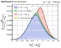
Refer to caption
Refer to caption
Figure 36: Distributions of (a) the estimator H4,2P~P~superscriptsubscript𝐻42~𝑃~𝑃H_{\mathrm{{\color[rgb]{0.1,0.1,0.44}\definecolor[named]{pgfstrokecolor}{rgb}{0.1,0.1,0.44}\textbf{4}}},\mathrm{{\color[rgb]{0.12,0.3,0.17}\definecolor[named]{pgfstrokecolor}{rgb}{0.12,0.3,0.17}\textbf{2}}}}^{\footnotesize\leavevmode\nobreak\ \mathrm{{\color[rgb]{0.45,0.0,0.09}\definecolor[named]{pgfstrokecolor}{rgb}{0.45,0.0,0.09}\textbf{$\tilde{P}\tilde{P}$}}}} and (b) H1,1P~P~superscriptsubscript𝐻11~𝑃~𝑃H_{\mathrm{{\color[rgb]{0.1,0.1,0.44}\definecolor[named]{pgfstrokecolor}{rgb}{0.1,0.1,0.44}\textbf{1}}},\mathrm{{\color[rgb]{0.12,0.3,0.17}\definecolor[named]{pgfstrokecolor}{rgb}{0.12,0.3,0.17}\textbf{1}}}}^{\footnotesize\leavevmode\nobreak\ \mathrm{{\color[rgb]{0.45,0.0,0.09}\definecolor[named]{pgfstrokecolor}{rgb}{0.45,0.0,0.09}\textbf{$\tilde{P}\tilde{P}$}}}} for simulated events corresponding to the processes described in Fig. 34. Each observable is appropriately normalized by true quantities.

The estimator H1,1P~P~superscriptsubscript𝐻11~𝑃~𝑃H_{\mathrm{{\color[rgb]{0.1,0.1,0.44}\definecolor[named]{pgfstrokecolor}{rgb}{0.1,0.1,0.44}\textbf{1}}},\mathrm{{\color[rgb]{0.12,0.3,0.17}\definecolor[named]{pgfstrokecolor}{rgb}{0.12,0.3,0.17}\textbf{1}}}}^{\footnotesize\leavevmode\nobreak\ \mathrm{{\color[rgb]{0.45,0.0,0.09}\definecolor[named]{pgfstrokecolor}{rgb}{0.45,0.0,0.09}\textbf{$\tilde{P}\tilde{P}$}}}} can be used to examine the same event at a coarser level of resolution, with distributions shown in Fig. 36(b). Using a subset of the information going into H4,2P~P~superscriptsubscript𝐻42~𝑃~𝑃H_{\mathrm{{\color[rgb]{0.1,0.1,0.44}\definecolor[named]{pgfstrokecolor}{rgb}{0.1,0.1,0.44}\textbf{4}}},\mathrm{{\color[rgb]{0.12,0.3,0.17}\definecolor[named]{pgfstrokecolor}{rgb}{0.12,0.3,0.17}\textbf{2}}}}^{\footnotesize\leavevmode\nobreak\ \mathrm{{\color[rgb]{0.45,0.0,0.09}\definecolor[named]{pgfstrokecolor}{rgb}{0.45,0.0,0.09}\textbf{$\tilde{P}\tilde{P}$}}}}, H1,1P~P~superscriptsubscript𝐻11~𝑃~𝑃H_{\mathrm{{\color[rgb]{0.1,0.1,0.44}\definecolor[named]{pgfstrokecolor}{rgb}{0.1,0.1,0.44}\textbf{1}}},\mathrm{{\color[rgb]{0.12,0.3,0.17}\definecolor[named]{pgfstrokecolor}{rgb}{0.12,0.3,0.17}\textbf{1}}}}^{\footnotesize\leavevmode\nobreak\ \mathrm{{\color[rgb]{0.45,0.0,0.09}\definecolor[named]{pgfstrokecolor}{rgb}{0.45,0.0,0.09}\textbf{$\tilde{P}\tilde{P}$}}}} is sensitive to the difference in invisible particle kinematics between the processes, reflecting the fraction of decay phase-space given to the neutralinos, with a kinematic limit at 2γMΔ2𝛾subscript𝑀Δ2\gamma M_{\Delta}, where γ=mP~P~/2mP~𝛾superscriptsubscript𝑚~𝑃~𝑃absent2superscriptsubscript𝑚~𝑃absent\gamma=m_{\footnotesize\mathrm{{\color[rgb]{0.45,0.0,0.09}\definecolor[named]{pgfstrokecolor}{rgb}{0.45,0.0,0.09}\textbf{$\tilde{P}\tilde{P}$}}}}^{\footnotesize\leavevmode\nobreak\ }/2m_{\footnotesize\mathrm{{\color[rgb]{0.45,0.0,0.09}\definecolor[named]{pgfstrokecolor}{rgb}{0.45,0.0,0.09}\textbf{$\tilde{P}$}}}}^{\footnotesize\leavevmode\nobreak\ } and MΔ=(mP~ 2mχ~0 2)/mP~subscript𝑀Δsuperscriptsubscript𝑚~𝑃2superscriptsubscript𝑚superscript~𝜒02superscriptsubscript𝑚~𝑃absentM_{\Delta}=(m_{\footnotesize\mathrm{{\color[rgb]{0.45,0.0,0.09}\definecolor[named]{pgfstrokecolor}{rgb}{0.45,0.0,0.09}\textbf{$\tilde{P}$}}}}^{\footnotesize\leavevmode\nobreak\ 2}-m_{\footnotesize\mathrm{{\color[rgb]{0.45,0.0,0.09}\definecolor[named]{pgfstrokecolor}{rgb}{0.45,0.0,0.09}\textbf{$\tilde{\chi}^{0}$}}}}^{\footnotesize\leavevmode\nobreak\ 2})/m_{\footnotesize\mathrm{{\color[rgb]{0.45,0.0,0.09}\definecolor[named]{pgfstrokecolor}{rgb}{0.45,0.0,0.09}\textbf{$\tilde{P}$}}}}^{\footnotesize\leavevmode\nobreak\ }. When the gluinos decay through an intermediate sbottom quark, the distribution of H1,1P~P~superscriptsubscript𝐻11~𝑃~𝑃H_{\mathrm{{\color[rgb]{0.1,0.1,0.44}\definecolor[named]{pgfstrokecolor}{rgb}{0.1,0.1,0.44}\textbf{1}}},\mathrm{{\color[rgb]{0.12,0.3,0.17}\definecolor[named]{pgfstrokecolor}{rgb}{0.12,0.3,0.17}\textbf{1}}}}^{\footnotesize\leavevmode\nobreak\ \mathrm{{\color[rgb]{0.45,0.0,0.09}\definecolor[named]{pgfstrokecolor}{rgb}{0.45,0.0,0.09}\textbf{$\tilde{P}\tilde{P}$}}}} becomes indistinguishable from direct sbottom production in the limit mb~mg~superscriptsubscript𝑚~𝑏absentsuperscriptsubscript𝑚~𝑔absentm_{\footnotesize\mathrm{{\color[rgb]{0.45,0.0,0.09}\definecolor[named]{pgfstrokecolor}{rgb}{0.45,0.0,0.09}\textbf{$\tilde{b}$}}}}^{\footnotesize\leavevmode\nobreak\ }\rightarrow m_{\footnotesize\mathrm{{\color[rgb]{0.45,0.0,0.09}\definecolor[named]{pgfstrokecolor}{rgb}{0.45,0.0,0.09}\textbf{$\tilde{g}$}}}}^{\footnotesize\leavevmode\nobreak\ }.

While the estimators H4,2P~P~superscriptsubscript𝐻42~𝑃~𝑃H_{\mathrm{{\color[rgb]{0.1,0.1,0.44}\definecolor[named]{pgfstrokecolor}{rgb}{0.1,0.1,0.44}\textbf{4}}},\mathrm{{\color[rgb]{0.12,0.3,0.17}\definecolor[named]{pgfstrokecolor}{rgb}{0.12,0.3,0.17}\textbf{2}}}}^{\footnotesize\leavevmode\nobreak\ \mathrm{{\color[rgb]{0.45,0.0,0.09}\definecolor[named]{pgfstrokecolor}{rgb}{0.45,0.0,0.09}\textbf{$\tilde{P}\tilde{P}$}}}} and H1,1P~P~superscriptsubscript𝐻11~𝑃~𝑃H_{\mathrm{{\color[rgb]{0.1,0.1,0.44}\definecolor[named]{pgfstrokecolor}{rgb}{0.1,0.1,0.44}\textbf{1}}},\mathrm{{\color[rgb]{0.12,0.3,0.17}\definecolor[named]{pgfstrokecolor}{rgb}{0.12,0.3,0.17}\textbf{1}}}}^{\footnotesize\leavevmode\nobreak\ \mathrm{{\color[rgb]{0.45,0.0,0.09}\definecolor[named]{pgfstrokecolor}{rgb}{0.45,0.0,0.09}\textbf{$\tilde{P}\tilde{P}$}}}} are constructed from momenta in the same reference frame, the information they contain is largely independent, as demonstrated in Fig. 37(a,b,c). The residual correlations between the observables are sensitive to the differences in gluino decays, with distinctive behavior for each.
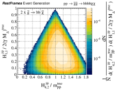
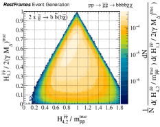
Refer to caption
Refer to caption
Refer to caption
Refer to caption
Refer to caption
Refer to caption
Figure 37: Distributions of the estimators (a,b,c) H1,1P~P~superscriptsubscript𝐻11~𝑃~𝑃H_{\mathrm{{\color[rgb]{0.1,0.1,0.44}\definecolor[named]{pgfstrokecolor}{rgb}{0.1,0.1,0.44}\textbf{1}}},\mathrm{{\color[rgb]{0.12,0.3,0.17}\definecolor[named]{pgfstrokecolor}{rgb}{0.12,0.3,0.17}\textbf{1}}}}^{\footnotesize\leavevmode\nobreak\ \mathrm{{\color[rgb]{0.45,0.0,0.09}\definecolor[named]{pgfstrokecolor}{rgb}{0.45,0.0,0.09}\textbf{$\tilde{P}\tilde{P}$}}}} and (d,e,f) H2,1P~a/H4,2P~P~superscriptsubscript𝐻21subscript~𝑃𝑎superscriptsubscript𝐻42~𝑃~𝑃H_{\mathrm{{\color[rgb]{0.1,0.1,0.44}\definecolor[named]{pgfstrokecolor}{rgb}{0.1,0.1,0.44}\textbf{2}}},\mathrm{{\color[rgb]{0.12,0.3,0.17}\definecolor[named]{pgfstrokecolor}{rgb}{0.12,0.3,0.17}\textbf{1}}}}^{\footnotesize\leavevmode\nobreak\ \mathrm{{\color[rgb]{0.45,0.0,0.09}\definecolor[named]{pgfstrokecolor}{rgb}{0.45,0.0,0.09}\textbf{$\tilde{P}_{a}$}}}}/H_{\mathrm{{\color[rgb]{0.1,0.1,0.44}\definecolor[named]{pgfstrokecolor}{rgb}{0.1,0.1,0.44}\textbf{4}}},\mathrm{{\color[rgb]{0.12,0.3,0.17}\definecolor[named]{pgfstrokecolor}{rgb}{0.12,0.3,0.17}\textbf{2}}}}^{\footnotesize\leavevmode\nobreak\ \mathrm{{\color[rgb]{0.45,0.0,0.09}\definecolor[named]{pgfstrokecolor}{rgb}{0.45,0.0,0.09}\textbf{$\tilde{P}\tilde{P}$}}}}, each as a function of H4,2P~P~/mP~P~superscriptsubscript𝐻42~𝑃~𝑃superscriptsubscript𝑚~𝑃~𝑃absentH_{\mathrm{{\color[rgb]{0.1,0.1,0.44}\definecolor[named]{pgfstrokecolor}{rgb}{0.1,0.1,0.44}\textbf{4}}},\mathrm{{\color[rgb]{0.12,0.3,0.17}\definecolor[named]{pgfstrokecolor}{rgb}{0.12,0.3,0.17}\textbf{2}}}}^{\footnotesize\leavevmode\nobreak\ \mathrm{{\color[rgb]{0.45,0.0,0.09}\definecolor[named]{pgfstrokecolor}{rgb}{0.45,0.0,0.09}\textbf{$\tilde{P}\tilde{P}$}}}}/m_{\footnotesize\mathrm{{\color[rgb]{0.45,0.0,0.09}\definecolor[named]{pgfstrokecolor}{rgb}{0.45,0.0,0.09}\textbf{$\tilde{P}\tilde{P}$}}}}^{\footnotesize\leavevmode\nobreak\ }, for simulated gluino pair production events corresponding to the decays described in Fig. 34. The figures correspond to (a,d) gluino three-body decays, (b,e) gluinos decaying through an intermediate, on-shell sbottom quark, and (c,f) mixed gluino decays. Each observable is normalized, when appropriate, by true quantities.

To better resolve the kinematics of the individual sparticles, the estimators H2,1P~asuperscriptsubscript𝐻21subscript~𝑃𝑎H_{\mathrm{{\color[rgb]{0.1,0.1,0.44}\definecolor[named]{pgfstrokecolor}{rgb}{0.1,0.1,0.44}\textbf{2}}},\mathrm{{\color[rgb]{0.12,0.3,0.17}\definecolor[named]{pgfstrokecolor}{rgb}{0.12,0.3,0.17}\textbf{1}}}}^{\footnotesize\leavevmode\nobreak\ \mathrm{{\color[rgb]{0.45,0.0,0.09}\definecolor[named]{pgfstrokecolor}{rgb}{0.45,0.0,0.09}\textbf{$\tilde{P}_{a}$}}}} and H2,1P~bsuperscriptsubscript𝐻21subscript~𝑃𝑏H_{\mathrm{{\color[rgb]{0.1,0.1,0.44}\definecolor[named]{pgfstrokecolor}{rgb}{0.1,0.1,0.44}\textbf{2}}},\mathrm{{\color[rgb]{0.12,0.3,0.17}\definecolor[named]{pgfstrokecolor}{rgb}{0.12,0.3,0.17}\textbf{1}}}}^{\footnotesize\leavevmode\nobreak\ \mathrm{{\color[rgb]{0.45,0.0,0.09}\definecolor[named]{pgfstrokecolor}{rgb}{0.45,0.0,0.09}\textbf{$\tilde{P}_{b}$}}}} can be used, which use partitions of only the visible and invisible particles associated with the hemispheres “a” and “b”, respectively. These observables are sensitive to the masses of these sparticles and, when compared to H4,2P~P~superscriptsubscript𝐻42~𝑃~𝑃H_{\mathrm{{\color[rgb]{0.1,0.1,0.44}\definecolor[named]{pgfstrokecolor}{rgb}{0.1,0.1,0.44}\textbf{4}}},\mathrm{{\color[rgb]{0.12,0.3,0.17}\definecolor[named]{pgfstrokecolor}{rgb}{0.12,0.3,0.17}\textbf{2}}}}^{\footnotesize\leavevmode\nobreak\ \mathrm{{\color[rgb]{0.45,0.0,0.09}\definecolor[named]{pgfstrokecolor}{rgb}{0.45,0.0,0.09}\textbf{$\tilde{P}\tilde{P}$}}}}, reveal the presence of the P~~𝑃\tilde{P} resonances, as can be seen in Fig. 37(d,e,f). When these Hn,mFsuperscriptsubscript𝐻𝑛𝑚FH_{\mathrm{{\color[rgb]{0.1,0.1,0.44}\definecolor[named]{pgfstrokecolor}{rgb}{0.1,0.1,0.44}\textbf{$n$}}},\mathrm{{\color[rgb]{0.12,0.3,0.17}\definecolor[named]{pgfstrokecolor}{rgb}{0.12,0.3,0.17}\textbf{$m$}}}}^{\footnotesize\leavevmode\nobreak\ \mathrm{{\color[rgb]{0.45,0.0,0.09}\definecolor[named]{pgfstrokecolor}{rgb}{0.45,0.0,0.09}\textbf{F}}}} variables are applied in ratio, like H2,1P~a/b/H4,2P~P~superscriptsubscript𝐻21subscript~𝑃𝑎𝑏superscriptsubscript𝐻42~𝑃~𝑃H_{\mathrm{{\color[rgb]{0.1,0.1,0.44}\definecolor[named]{pgfstrokecolor}{rgb}{0.1,0.1,0.44}\textbf{2}}},\mathrm{{\color[rgb]{0.12,0.3,0.17}\definecolor[named]{pgfstrokecolor}{rgb}{0.12,0.3,0.17}\textbf{1}}}}^{\footnotesize\leavevmode\nobreak\ \mathrm{{\color[rgb]{0.45,0.0,0.09}\definecolor[named]{pgfstrokecolor}{rgb}{0.45,0.0,0.09}\textbf{$\tilde{P}_{a/b}$}}}}/H_{\mathrm{{\color[rgb]{0.1,0.1,0.44}\definecolor[named]{pgfstrokecolor}{rgb}{0.1,0.1,0.44}\textbf{4}}},\mathrm{{\color[rgb]{0.12,0.3,0.17}\definecolor[named]{pgfstrokecolor}{rgb}{0.12,0.3,0.17}\textbf{2}}}}^{\footnotesize\leavevmode\nobreak\ \mathrm{{\color[rgb]{0.45,0.0,0.09}\definecolor[named]{pgfstrokecolor}{rgb}{0.45,0.0,0.09}\textbf{$\tilde{P}\tilde{P}$}}}}, they indicate whether there is a resonant structure between the two different pairs of partitions considered. In the case of the center-of-mass system, P~P~~𝑃~𝑃\tilde{P}\tilde{P}, “decaying” to the individual sparticles, this structure is clearly visible in Fig. 37, and is estimated with little correlation to the total mass scale, H4,2P~P~superscriptsubscript𝐻42~𝑃~𝑃H_{\mathrm{{\color[rgb]{0.1,0.1,0.44}\definecolor[named]{pgfstrokecolor}{rgb}{0.1,0.1,0.44}\textbf{4}}},\mathrm{{\color[rgb]{0.12,0.3,0.17}\definecolor[named]{pgfstrokecolor}{rgb}{0.12,0.3,0.17}\textbf{2}}}}^{\footnotesize\leavevmode\nobreak\ \mathrm{{\color[rgb]{0.45,0.0,0.09}\definecolor[named]{pgfstrokecolor}{rgb}{0.45,0.0,0.09}\textbf{$\tilde{P}\tilde{P}$}}}}. Only small differences in the distributions of these ratios are observed between the different gluino decays considered.

As multiple decays of the gluinos are being considered simultaneously, we take an agnostic approach to the parameterization of observables describing their decays, defining additional estimators H1,1P~asuperscriptsubscript𝐻11subscript~𝑃𝑎H_{\mathrm{{\color[rgb]{0.1,0.1,0.44}\definecolor[named]{pgfstrokecolor}{rgb}{0.1,0.1,0.44}\textbf{1}}},\mathrm{{\color[rgb]{0.12,0.3,0.17}\definecolor[named]{pgfstrokecolor}{rgb}{0.12,0.3,0.17}\textbf{1}}}}^{\footnotesize\leavevmode\nobreak\ \mathrm{{\color[rgb]{0.45,0.0,0.09}\definecolor[named]{pgfstrokecolor}{rgb}{0.45,0.0,0.09}\textbf{$\tilde{P}_{a}$}}}} and H1,1P~bsuperscriptsubscript𝐻11subscript~𝑃𝑏H_{\mathrm{{\color[rgb]{0.1,0.1,0.44}\definecolor[named]{pgfstrokecolor}{rgb}{0.1,0.1,0.44}\textbf{1}}},\mathrm{{\color[rgb]{0.12,0.3,0.17}\definecolor[named]{pgfstrokecolor}{rgb}{0.12,0.3,0.17}\textbf{1}}}}^{\footnotesize\leavevmode\nobreak\ \mathrm{{\color[rgb]{0.45,0.0,0.09}\definecolor[named]{pgfstrokecolor}{rgb}{0.45,0.0,0.09}\textbf{$\tilde{P}_{b}$}}}}. These correspond to partial abstractions of the gluino decays, where each visible system Va/b is treated as only one particle, such that, taken in ratio with their respective H2,1P~a/bsuperscriptsubscript𝐻21subscript~𝑃𝑎𝑏H_{\mathrm{{\color[rgb]{0.1,0.1,0.44}\definecolor[named]{pgfstrokecolor}{rgb}{0.1,0.1,0.44}\textbf{2}}},\mathrm{{\color[rgb]{0.12,0.3,0.17}\definecolor[named]{pgfstrokecolor}{rgb}{0.12,0.3,0.17}\textbf{1}}}}^{\footnotesize\leavevmode\nobreak\ \mathrm{{\color[rgb]{0.45,0.0,0.09}\definecolor[named]{pgfstrokecolor}{rgb}{0.45,0.0,0.09}\textbf{$\tilde{P}_{a/b}$}}}}, they are sensitive to the gluino decay structure. The distributions of these ratios are shown in Fig. 38 for each gluino decay, and for each reconstructed hemisphere of the event. We adopt the convention that the hemisphere assigned the highest transverse momentum jet coming from the true gluino “a” decay in reconstruction is also assigned the label “a” which, in the mixed decay case, corresponds to a decay through an on-shell sbottom quark. The distributions of the ratio H1,1P~a/b/H2,1P~a/bsuperscriptsubscript𝐻11subscript~𝑃𝑎𝑏superscriptsubscript𝐻21subscript~𝑃𝑎𝑏H_{\mathrm{{\color[rgb]{0.1,0.1,0.44}\definecolor[named]{pgfstrokecolor}{rgb}{0.1,0.1,0.44}\textbf{1}}},\mathrm{{\color[rgb]{0.12,0.3,0.17}\definecolor[named]{pgfstrokecolor}{rgb}{0.12,0.3,0.17}\textbf{1}}}}^{\footnotesize\leavevmode\nobreak\ \mathrm{{\color[rgb]{0.45,0.0,0.09}\definecolor[named]{pgfstrokecolor}{rgb}{0.45,0.0,0.09}\textbf{$\tilde{P}_{a/b}$}}}}/H_{\mathrm{{\color[rgb]{0.1,0.1,0.44}\definecolor[named]{pgfstrokecolor}{rgb}{0.1,0.1,0.44}\textbf{2}}},\mathrm{{\color[rgb]{0.12,0.3,0.17}\definecolor[named]{pgfstrokecolor}{rgb}{0.12,0.3,0.17}\textbf{1}}}}^{\footnotesize\leavevmode\nobreak\ \mathrm{{\color[rgb]{0.45,0.0,0.09}\definecolor[named]{pgfstrokecolor}{rgb}{0.45,0.0,0.09}\textbf{$\tilde{P}_{a/b}$}}}} have a distinct shape indicative of the type of decay, with the observables corresponding to the different gluino decays in the mixed case each adopting shapes closely resembling those of the symmetric cases.
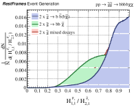
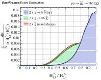
Refer to caption
Refer to caption
Figure 38: Distributions of (a) the estimator H1,1P~a/H2,1P~asuperscriptsubscript𝐻11subscript~𝑃𝑎superscriptsubscript𝐻21subscript~𝑃𝑎H_{\mathrm{{\color[rgb]{0.1,0.1,0.44}\definecolor[named]{pgfstrokecolor}{rgb}{0.1,0.1,0.44}\textbf{1}}},\mathrm{{\color[rgb]{0.12,0.3,0.17}\definecolor[named]{pgfstrokecolor}{rgb}{0.12,0.3,0.17}\textbf{1}}}}^{\footnotesize\leavevmode\nobreak\ \mathrm{{\color[rgb]{0.45,0.0,0.09}\definecolor[named]{pgfstrokecolor}{rgb}{0.45,0.0,0.09}\textbf{$\tilde{P}_{a}$}}}}/H_{\mathrm{{\color[rgb]{0.1,0.1,0.44}\definecolor[named]{pgfstrokecolor}{rgb}{0.1,0.1,0.44}\textbf{2}}},\mathrm{{\color[rgb]{0.12,0.3,0.17}\definecolor[named]{pgfstrokecolor}{rgb}{0.12,0.3,0.17}\textbf{1}}}}^{\footnotesize\leavevmode\nobreak\ \mathrm{{\color[rgb]{0.45,0.0,0.09}\definecolor[named]{pgfstrokecolor}{rgb}{0.45,0.0,0.09}\textbf{$\tilde{P}_{a}$}}}}, and (b) H1,1P~b/H2,1P~bsuperscriptsubscript𝐻11subscript~𝑃𝑏superscriptsubscript𝐻21subscript~𝑃𝑏H_{\mathrm{{\color[rgb]{0.1,0.1,0.44}\definecolor[named]{pgfstrokecolor}{rgb}{0.1,0.1,0.44}\textbf{1}}},\mathrm{{\color[rgb]{0.12,0.3,0.17}\definecolor[named]{pgfstrokecolor}{rgb}{0.12,0.3,0.17}\textbf{1}}}}^{\footnotesize\leavevmode\nobreak\ \mathrm{{\color[rgb]{0.45,0.0,0.09}\definecolor[named]{pgfstrokecolor}{rgb}{0.45,0.0,0.09}\textbf{$\tilde{P}_{b}$}}}}/H_{\mathrm{{\color[rgb]{0.1,0.1,0.44}\definecolor[named]{pgfstrokecolor}{rgb}{0.1,0.1,0.44}\textbf{2}}},\mathrm{{\color[rgb]{0.12,0.3,0.17}\definecolor[named]{pgfstrokecolor}{rgb}{0.12,0.3,0.17}\textbf{1}}}}^{\footnotesize\leavevmode\nobreak\ \mathrm{{\color[rgb]{0.45,0.0,0.09}\definecolor[named]{pgfstrokecolor}{rgb}{0.45,0.0,0.09}\textbf{$\tilde{P}_{b}$}}}}, for simulated gluino pair production events corresponding to the decays described in Fig. 34. In the case of events with mixed gluino decays, “a” is associated with the intermediate sbottom quark while “b” corresponds to the three-body decay.

The partitioning of information throughout the event reconstruction and observable definition allows for the ratios H1,1P~a/b/H2,1P~a/bsuperscriptsubscript𝐻11subscript~𝑃𝑎𝑏superscriptsubscript𝐻21subscript~𝑃𝑎𝑏H_{\mathrm{{\color[rgb]{0.1,0.1,0.44}\definecolor[named]{pgfstrokecolor}{rgb}{0.1,0.1,0.44}\textbf{1}}},\mathrm{{\color[rgb]{0.12,0.3,0.17}\definecolor[named]{pgfstrokecolor}{rgb}{0.12,0.3,0.17}\textbf{1}}}}^{\footnotesize\leavevmode\nobreak\ \mathrm{{\color[rgb]{0.45,0.0,0.09}\definecolor[named]{pgfstrokecolor}{rgb}{0.45,0.0,0.09}\textbf{$\tilde{P}_{a/b}$}}}}/H_{\mathrm{{\color[rgb]{0.1,0.1,0.44}\definecolor[named]{pgfstrokecolor}{rgb}{0.1,0.1,0.44}\textbf{2}}},\mathrm{{\color[rgb]{0.12,0.3,0.17}\definecolor[named]{pgfstrokecolor}{rgb}{0.12,0.3,0.17}\textbf{1}}}}^{\footnotesize\leavevmode\nobreak\ \mathrm{{\color[rgb]{0.45,0.0,0.09}\definecolor[named]{pgfstrokecolor}{rgb}{0.45,0.0,0.09}\textbf{$\tilde{P}_{a/b}$}}}} to be estimated independently for each half of the event, as shown in Fig. 39. The small asymmetries in these distributions for the symmetric decays is a result of the convention for assigning the labels “a” and “b” to the two halves of the event, and appears when the combinatoric assignment of the b𝑏b-tagged jets is incorrect in the reconstruction. Otherwise, the H1,1P~a/b/H2,1P~a/bsuperscriptsubscript𝐻11subscript~𝑃𝑎𝑏superscriptsubscript𝐻21subscript~𝑃𝑎𝑏H_{\mathrm{{\color[rgb]{0.1,0.1,0.44}\definecolor[named]{pgfstrokecolor}{rgb}{0.1,0.1,0.44}\textbf{1}}},\mathrm{{\color[rgb]{0.12,0.3,0.17}\definecolor[named]{pgfstrokecolor}{rgb}{0.12,0.3,0.17}\textbf{1}}}}^{\footnotesize\leavevmode\nobreak\ \mathrm{{\color[rgb]{0.45,0.0,0.09}\definecolor[named]{pgfstrokecolor}{rgb}{0.45,0.0,0.09}\textbf{$\tilde{P}_{a/b}$}}}}/H_{\mathrm{{\color[rgb]{0.1,0.1,0.44}\definecolor[named]{pgfstrokecolor}{rgb}{0.1,0.1,0.44}\textbf{2}}},\mathrm{{\color[rgb]{0.12,0.3,0.17}\definecolor[named]{pgfstrokecolor}{rgb}{0.12,0.3,0.17}\textbf{1}}}}^{\footnotesize\leavevmode\nobreak\ \mathrm{{\color[rgb]{0.45,0.0,0.09}\definecolor[named]{pgfstrokecolor}{rgb}{0.45,0.0,0.09}\textbf{$\tilde{P}_{a/b}$}}}} distribution for the g~bb~~𝑔𝑏~𝑏\tilde{g}\rightarrow b\tilde{b} decay in the mixed case resembles that of the symmetric decay case, as it independently does for the three-body decay in the opposite event hemisphere.
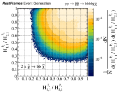
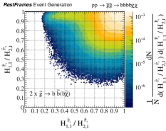
Refer to caption
Refer to caption
Refer to caption
Figure 39: Distributions of H1,1P~a/H2,1P~asuperscriptsubscript𝐻11subscript~𝑃𝑎superscriptsubscript𝐻21subscript~𝑃𝑎H_{\mathrm{{\color[rgb]{0.1,0.1,0.44}\definecolor[named]{pgfstrokecolor}{rgb}{0.1,0.1,0.44}\textbf{1}}},\mathrm{{\color[rgb]{0.12,0.3,0.17}\definecolor[named]{pgfstrokecolor}{rgb}{0.12,0.3,0.17}\textbf{1}}}}^{\footnotesize\leavevmode\nobreak\ \mathrm{{\color[rgb]{0.45,0.0,0.09}\definecolor[named]{pgfstrokecolor}{rgb}{0.45,0.0,0.09}\textbf{$\tilde{P}_{a}$}}}}/H_{\mathrm{{\color[rgb]{0.1,0.1,0.44}\definecolor[named]{pgfstrokecolor}{rgb}{0.1,0.1,0.44}\textbf{2}}},\mathrm{{\color[rgb]{0.12,0.3,0.17}\definecolor[named]{pgfstrokecolor}{rgb}{0.12,0.3,0.17}\textbf{1}}}}^{\footnotesize\leavevmode\nobreak\ \mathrm{{\color[rgb]{0.45,0.0,0.09}\definecolor[named]{pgfstrokecolor}{rgb}{0.45,0.0,0.09}\textbf{$\tilde{P}_{a}$}}}}, as a function of H1,1P~b/H2,1P~bsuperscriptsubscript𝐻11subscript~𝑃𝑏superscriptsubscript𝐻21subscript~𝑃𝑏H_{\mathrm{{\color[rgb]{0.1,0.1,0.44}\definecolor[named]{pgfstrokecolor}{rgb}{0.1,0.1,0.44}\textbf{1}}},\mathrm{{\color[rgb]{0.12,0.3,0.17}\definecolor[named]{pgfstrokecolor}{rgb}{0.12,0.3,0.17}\textbf{1}}}}^{\footnotesize\leavevmode\nobreak\ \mathrm{{\color[rgb]{0.45,0.0,0.09}\definecolor[named]{pgfstrokecolor}{rgb}{0.45,0.0,0.09}\textbf{$\tilde{P}_{b}$}}}}/H_{\mathrm{{\color[rgb]{0.1,0.1,0.44}\definecolor[named]{pgfstrokecolor}{rgb}{0.1,0.1,0.44}\textbf{2}}},\mathrm{{\color[rgb]{0.12,0.3,0.17}\definecolor[named]{pgfstrokecolor}{rgb}{0.12,0.3,0.17}\textbf{1}}}}^{\footnotesize\leavevmode\nobreak\ \mathrm{{\color[rgb]{0.45,0.0,0.09}\definecolor[named]{pgfstrokecolor}{rgb}{0.45,0.0,0.09}\textbf{$\tilde{P}_{b}$}}}}, for simulated gluino pair production events corresponding to the decays described in Fig. 34. The figures correspond to (a) gluino three-body decays, (b) gluinos decaying through an intermediate, on-shell sbottom quark, and (c) mixed gluino decays. In this case of events with mixed gluino decays, “a” is associated with the intermediate sbottom quark while “b” corresponds to the three-body decay. The small lack of symmetry between otherwise symmetric decays observed in the distributions (a,b) is a result of the convention that the true b2a is always associated with the reconstructed “a” hemisphere and incorrect combinatoric assignments.

The basis of observables produced when partitioning the information contained in each reconstructed event into approximately uncorrelated variables through the RJR approach is useful for not just studying these types of decay topologies, but searching for evidence of these phenomena in experimental data. By independently maintaining sensitivity to each decay in the event, background processes must simultaneously fake many different kinematic features in order to be confused with signal. This includes not only the total mass scale of the event, but how energy is shared between the products of each subsequent decay. That these observables are able to distinguish between the different decays of similar sparticles indicates that they are also sensitive to expected differences in SM backgrounds, where the absence of the same resonance structure in the events can be exploited.

IX Summary

As evidenced by the examples discussed in this paper, many of the final state topologies of interest at particle colliders contain both kinematic and combinatoric ambiguities, with missing information resulting from invisible or indistinguishable particles. Recursive Jigsaw Reconstruction is a systematic prescription for overcoming these unknowns, and approximately reconstructing each event in its entirety, resulting in a basis of kinematic estimators sensitive to the masses and decay angles of all the particles appearing in them.

This is accomplished by factorizing all of the unknowns appearing in an event according to which intermediate decays they are related to, and using the library of Jigsaw Rules, interchangeable and configurable algorithms for determining these unknowns, to resolve them while recursively moving through the decay tree describing the event. The JR’s for analyzing events with one invisible particle, like Wν𝑊𝜈W\rightarrow\ell\nu in Section V.1, tbW(ν)𝑡𝑏𝑊𝜈t\rightarrow bW(\ell\nu) in Section V.2, and H±h(γγ)W±(ν)superscript𝐻plus-or-minus𝛾𝛾superscript𝑊plus-or-minus𝜈H^{\pm}\rightarrow h(\gamma\gamma)W^{\pm}(\ell\nu) in Section V.3, can be combined with more complicated ones in events with multiple invisible particle.

In events with two invisible particles coming from symmetrically similar decays, an array of different contra-boost invariant JR’s can be used to analyze processes like HW(ν)W(ν)𝐻𝑊𝜈𝑊𝜈H\rightarrow W(\ell\nu)W(\ell\nu) in Section VI.1, t~t~tχ~10tχ~10~𝑡~𝑡𝑡subscriptsuperscript~𝜒01𝑡subscriptsuperscript~𝜒01\tilde{t}\tilde{t}\rightarrow t\tilde{\chi}^{0}_{1}t\tilde{\chi}^{0}_{1} in Section VI.2, and χ~20χ~20h(γγ)χ~10Z()χ~10subscriptsuperscript~𝜒02subscriptsuperscript~𝜒02𝛾𝛾subscriptsuperscript~𝜒01𝑍subscriptsuperscript~𝜒01\tilde{\chi}^{0}_{2}\tilde{\chi}^{0}_{2}\rightarrow h(\gamma\gamma)\tilde{\chi}^{0}_{1}Z(\ell\ell)\tilde{\chi}^{0}_{1} in Section VI.3. In these cases, both the mass of the total interaction and pair-produced massive particles can be independently determiend with the RJR approach. When there are even more intermediate particles appearing in the final state, like tt¯bW(ν)bW(ν)𝑡¯𝑡𝑏𝑊𝜈𝑏𝑊𝜈t\bar{t}\rightarrow bW(\ell\nu)bW(\ell\nu) in Sections VII.1 and VII.2, or t~t~bχ~±(ν~)bχ~(ν~)~𝑡~𝑡𝑏superscript~𝜒plus-or-minus~𝜈𝑏superscript~𝜒minus-or-plus~𝜈\tilde{t}\tilde{t}\rightarrow b\tilde{\chi}^{\pm}(\ell\tilde{\nu})b\tilde{\chi}^{\mp}(\ell\tilde{\nu}) in Section VII.3, estimators sensitive to the masses and decays of these additional particles are also determined.

There are JR’s for arbitrarily complex decays, like non-resonant N×W(ν)𝑁𝑊𝜈N\times W(\ell\nu) production in Section VIII.1. But the real strength of the RJR algorithm is that each of the JR’s is designed to only use the momentum of abstractions of the particles in each decay step, where multiple particles that are resolved in later decays are treated as indivisible single particles. This means that many JR’s can be combined, recursively, to analyze complicated events like Hhh4W(ν)𝐻4𝑊𝜈H\rightarrow hh\rightarrow 4W(\ell\nu) in Section VIII.2 with many invisible particles, or g~g~bbχ~10bbχ~10~𝑔~𝑔𝑏𝑏subscriptsuperscript~𝜒01𝑏𝑏subscriptsuperscript~𝜒01\tilde{g}\tilde{g}\rightarrow bb\tilde{\chi}^{0}_{1}bb\tilde{\chi}^{0}_{1} in Section VIII.3 with many indistinguishable particles.

The recursive, factorized, application of JR’s when analyzing events yields a complete basis of kinematic observables, each corresponding to quantities of interest in the event and largely independent of the others. With the library of JR’s described in this paper, the RJR algorithm can be used to provide such a basis for any decay topology imaginable, with the effective resolution of the corresponding estimators limited only by the measurements made in the detector and the imagination of analysts in choosing and assembling the JR pieces.

Acknowledgements.
The authors would like to thank the Harvard Club of Australia for the award of the “Australia-Harvard Fellowship” in 2014 and 2015 which made part of this work possible. PJ is supported by the Australian Research Council Future Fellowship FT130100018. CR wishes to thank the Harvard Society of Fellows and William F. Milton Fund for their generous support.

References

  • (1) Christoph Borschensky, Michael Kramer, Anna Kulesza, Michelangelo Mangano, Sanjay Padhi, Tilman Plehn, and Xavier Portell. Squark and gluino production cross sections in pp collisions at s𝑠\sqrt{s} = 13, 14, 33 and 100 TeV. Eur. Phys. J. C, 74:3174, 2014.
  • (2) Yu. A. Golfand and E. P. Likhtman. Extension of the Algebra of Poincare Group Generators and Violation of p Invariance. JETP Lett., 13:323–326, 1971. [Pisma Zh. Eksp. Teor. Fiz.13,452(1971)].
  • (3) A. Neveu and J. H. Schwarz. Factorizable dual model of pions. Nucl. Phys., B31:86–112, 1971.
  • (4) Pierre Ramond. Dual Theory for Free Fermions. Phys. Rev., D3:2415–2418, 1971.
  • (5) D. V. Volkov and V. P. Akulov. Is the Neutrino a Goldstone Particle? Phys. Lett. B, 46:109–110, 1973.
  • (6) J. Wess and B. Zumino. Supergauge Transformations in Four-Dimensions. Nucl. Phys. B, 70:39–50, 1974.
  • (7) Abdus Salam and J. A. Strathdee. Supersymmetry and Nonabelian Gauges. Phys. Lett. B, 51:353–355, 1974.
  • (8) J. Wess and B. Zumino. Supergauge Invariant Extension of Quantum Electrodynamics. Nucl. Phys. B, 78:1, 1974.
  • (9) S. Ferrara and B. Zumino. Supergauge Invariant Yang-Mills Theories. Nucl. Phys. B, 79:413, 1974.
  • (10) Stephen P. Martin. A Supersymmetry primer. Adv. Ser. Direct. High Energy Phys., 18,1, 1998.
  • (11) Christopher Lester and Alan Barr. MTGEN: Mass scale measurements in pair-production at colliders. JHEP, 12:102, 2007.
  • (12) Graham G. Ross and Mario Serna. Mass determination of new states at hadron colliders. Phys. Lett., B665:212–218, 2008.
  • (13) Won Sang Cho, Kiwoon Choi, Yeong Gyun Kim, and Chan Beom Park. Gluino Stransverse Mass. Phys. Rev. Lett., 100:171801, 2008.
  • (14) Won Sang Cho, Kiwoon Choi, Yeong Gyun Kim, and Chan Beom Park. Measuring superparticle masses at hadron collider using the transverse mass kink. JHEP, 02:035, 2008.
  • (15) Ben Gripaios. Transverse observables and mass determination at hadron colliders. JHEP, 02:053, 2008.
  • (16) Alan J. Barr, Ben Gripaios, and Christopher G. Lester. Weighing Wimps with Kinks at Colliders: Invisible Particle Mass Measurements from Endpoints. JHEP, 02:014, 2008.
  • (17) Hsin-Chia Cheng and Zhenyu Han. Minimal Kinematic Constraints and m(T2). JHEP, 12:063, 2008.
  • (18) Won Sang Cho, Kiwoon Choi, Yeong Gyun Kim, and Chan Beom Park. Measuring the top quark mass with m(T2) at the LHC. Phys. Rev., D78:034019, 2008.
  • (19) Daniel R. Tovey. On measuring the masses of pair-produced semi-invisibly decaying particles at hadron colliders. JHEP, 04:034, 2008.
  • (20) Mihoko M. Nojiri, Kazuki Sakurai, Yasuhiro Shimizu, and Michihisa Takeuchi. Handling jets + missing E(T) channel using inclusive m(T2). JHEP, 10:100, 2008.
  • (21) Mihoko M. Nojiri, Yasuhiro Shimizu, Shogo Okada, and Kiyotomo Kawagoe. Inclusive transverse mass analysis for squark and gluino mass determination. JHEP, 06:035, 2008.
  • (22) Alan J. Barr, Graham G. Ross, and Mario Serna. The Precision Determination of Invisible-Particle Masses at the LHC. Phys. Rev., D78:056006, 2008.
  • (23) Alan J. Barr, Alex Pinder, and Mario Serna. Precision Determination of Invisible-Particle Masses at the CERN LHC. II. Phys. Rev., D79:074005, 2009.
  • (24) Won Sang Cho, Kiwoon Choi, Yeong Gyun Kim, and Chan Beom Park. M(T2)-assisted on-shell reconstruction of missing momenta and its application to spin measurement at the LHC. Phys. Rev., D79:031701, 2009.
  • (25) Michael Burns, Kyoungchul Kong, Konstantin T. Matchev, and Myeonghun Park. Using Subsystem MT2 for Complete Mass Determinations in Decay Chains with Missing Energy at Hadron Colliders. JHEP, 03:143, 2009.
  • (26) Partha Konar, Kyoungchul Kong, and Konstantin T. Matchev. s^minsubscript^𝑠𝑚𝑖𝑛\sqrt{\hat{s}}_{min} : A Global inclusive variable for determining the mass scale of new physics in events with missing energy at hadron colliders. JHEP, 03:085, 2009.
  • (27) Sung-Gi Kim, Nobuhiro Maekawa, Keiko I. Nagao, Mihoko M. Nojiri, and Kazuki Sakurai. LHC signature of supersymmetric models with non-universal sfermion masses. JHEP, 10:005, 2009.
  • (28) Alan J. Barr and Claire Gwenlan. The Race for supersymmetry: Using m(T2) for discovery. Phys. Rev., D80:074007, 2009.
  • (29) Johan Alwall, Kenji Hiramatsu, Mihoko M. Nojiri, and Yasuhiro Shimizu. Novel reconstruction technique for New Physics processes with initial state radiation. Phys. Rev. Lett., 103:151802, 2009.
  • (30) Alan J. Barr, Ben Gripaios, and Christopher G. Lester. Transverse masses and kinematic constraints: from the boundary to the crease. JHEP, 11:096, 2009.
  • (31) Partha Konar, Kyoungchul Kong, Konstantin T. Matchev, and Myeonghun Park. Superpartner Mass Measurement Technique using 1D Orthogonal Decompositions of the Cambridge Transverse Mass Variable MT2subscript𝑀𝑇2M_{T2}. Phys. Rev. Lett., 105:051802, 2010.
  • (32) Tao Han, Ian-Woo Kim, and Jeonghyeon Song. Kinematic Cusps: Determining the Missing Particle Mass at Colliders. Phys. Lett., B693:575–579, 2010.
  • (33) Won Sang Cho, Jihn E. Kim, and Ji-Hun Kim. Amplification of endpoint structure for new particle mass measurement at the LHC. Phys. Rev., D81:095010, 2010.
  • (34) Alan J. Barr and Christopher G. Lester. A Review of the Mass Measurement Techniques proposed for the Large Hadron Collider. J. Phys., G37:123001, 2010.
  • (35) Tao Han, Ian-Woo Kim, and Jeonghyeon Song. Kinematic Cusps With Two Missing Particles I: Antler Decay Topology. Phys. Rev., D87(3):035003, 2013.
  • (36) Tao Han, Ian-Woo Kim, and Jeonghyeon Song. Kinematic Cusps with Two Missing Particles II: Cascade Decay Topology. Phys. Rev., D87(3):035004, 2013.
  • (37) Ben Gripaios, Kazuki Sakurai, and Bryan Webber. Polynomials, Riemann surfaces, and reconstructing missing-energy events. JHEP, 09:140, 2011.
  • (38) Christopher Rogan. Kinematical variables towards new dynamics at the LHC. arXiv:1006.2727, 2010.
  • (39) C. G. Lester and D. J. Summers. Measuring masses of semi-invisibly decaying particles pair produced at hadron colliders. Phys. Lett., B463:99–103, 1999.
  • (40) Alan Barr, Christopher Lester, and P. Stephens. m(T2): The Truth behind the glamour. J. Phys., G29:2343–2363, 2003.
  • (41) Mihoko M. Nojiri, Giacomo Polesello, and Daniel R. Tovey. A Hybrid method for determining SUSY particle masses at the LHC with fully identified cascade decays. JHEP, 05:014, 2008.
  • (42) Giacomo Polesello and Daniel R. Tovey. Supersymmetric particle mass measurement with the boost-corrected contransverse mass. JHEP, 03:030, 2010.
  • (43) Ian-Woo Kim. Algebraic Singularity Method for Mass Measurement with Missing Energy. Phys. Rev. Lett., 104:081601, 2010.
  • (44) Christopher Rogan. RestFrames software library for hep event analysis. http://www.RestFrames.com, 2016.
  • (45) A. D. Martin, W. J. Stirling, R. S. Thorne, and G. Watt. Parton distributions for the LHC. Eur. Phys. J., C63:189–285, 2009.
  • (46) Matthew R. Buckley, Joseph D. Lykken, Christopher Rogan, and Maria Spiropulu. Super-Razor and Searches for Sleptons and Charginos at the LHC. Phys. Rev., D89(5):055020, 2014.
  • (47) Peter H. Schönemann. A generalized solution of the orthogonal procrustes problem. Psychometrika, 31(1):1–10, 1966.
  • (48) Paul Jackson, Christopher Rogan, and Marco Santoni. Sparticles in motion: Analyzing compressed SUSY scenarios with a new method of event reconstruction. Phys. Rev., D95(3):035031, 2017.