Lagrangian perturbation theory for modified gravity

Alejandro Aviles avilescervantes@gmail.com Departamento de Física, Instituto Nacional de Investigaciones Nucleares, Apartado Postal 18-1027, Col. Escandón, Ciudad de México,11801, México. Consejo Nacional de Ciencia y Tecnología, Av. Insurgentes Sur 1582, Colonia Crédito Constructor, Del. Benito Jurez, 03940, Ciudad de México, México    Jorge L. Cervantes-Cota jorge.cervantes@inin.gob.mx Departamento de Física, Instituto Nacional de Investigaciones Nucleares, Apartado Postal 18-1027, Col. Escandón, Ciudad de México,11801, México.
Abstract

We present a formalism to compute Lagrangian displacement fields for a wide range of cosmologies in the context of perturbation theory up to third order. We emphasize the case of theories with scale dependent gravitational strengths, such as chameleons, but our formalism can be accommodated to other modified gravity theories. In the non-linear regime two qualitative features arise. One, as is well known, is that nonlinearities lead to a screening of the force mediated by the scalar field. The second is a consequence of the transformation of the Klein-Gordon equation from Eulerian to Lagrangian coordinates, producing frame-lagging terms that are important especially at large scales, and if not considered, the theory does not reduce to the ΛΛ\LambdaCDM model in that limit. We apply our formalism to compute the 1-loop power spectrum and the correlation function in f(R)𝑓𝑅f(R) gravity by using different resummation schemes. We further discuss the IR divergences of these formalisms.

pacs:
PACS

I Introduction

General Relativity (GR) is the most successful theory of gravity we have nowadays. Indeed, it has passed so far all experimental tests ranging from 1μ𝜇\mum to 1 AU 1011similar-toabsentsuperscript1011\sim 10^{11}m Will:2014kxa ; Berti:2015itd . Nevertheless, mainly since the discovery of the accelerated expansion of the universe Perlmutter:1998np ; Riess:1998cb , concerns about its validity at cosmological scales have arisen. In addition, with the recent and forthcoming advent of a lot of cosmological data, especially from modern surveys Beutler:2016ixs ; Garcia-Fernandez:2016oud ; Aghamousa:2016zmz ; Racca:2016qpi ; Abell:2009aa , there is an increasing interest to test gravity at cosmological scales.

The minimal modification to the Einstein-Hilbert action compatible with the principle of generalized covariance —and the only that introduces no additional degrees of freedom— is provided by the introduction of a cosmological constant; this leads to the standard model of Cosmology, the ΛΛ\LambdaCDM model, that can explain the cosmic background radiation anisotropies with exquisite precision Ade:2015xua , the late time background evolution probed by measurements of the baryon acoustic oscillations (BAO) and supernova distance-redshift relations Betoule:2014frx , among several other observations. But this success comes with a price, the ΛΛ\Lambda side of the theory suffers from the smallness and coincidence problems Weinberg:1988cp ; Martin:2012bt . One alternative to the cosmological constant is that of evolving dark energy, in which exotic matter fields endowed with a negative pressure counteract the gravitational attraction and generate the cosmic acceleration Ratra:1987rm ; Tsujikawa:2010sc . From the observational point of view, a practical inconvenience of evolving dark energy is that a background expansion of the Universe that is close to ΛΛ\LambdaCDM implies that collapse features are nearly indistinguishable as well, as long as the dark energy is stress-free, and as a consequence it would be difficult to call the correct theory Bertschinger:2006aw ; Bertschinger:2008zb . The case of Modified Gravity (MG) is different because the two scalar gravitational potentials of the metric are not necessarily equal even in the absence of stress sources, and therefore a theory that mimics a dark energy model at the background level can predict a very different structure formation history.

The construction of alternatives theories of gravity has been a difficult endeavor because they are restricted to reduce to GR in some limits, while still having an impact on cosmic scales in order to provide the cosmic acceleration. For this reason, cosmologists have concentrated in gravitational theories that poses a screening mechanism Khoury:2010xi . In theories with one additional degree of freedom this can be achieved by the non-linearities of its evolution equation —the Klein-Gordon equation in the case of a scalar field. The general idea is that in regions with high density or large gradients of it, the additional (the fifth) force becomes negligible, recovering GR. These effects can be achieved by the scalar field itself or by its spatial derivatives, leading to different types of screenings: as, for example, the chameleon Khoury:2003aq ; khoury:2003rn , kinetic Babichev:2009ee , or Vainshtein Vainshtein:1972sx mechanisms.

In this work we are interested in the formation of cosmological structures at large scales. In the standard scenario, this process is driven by gravitational collapse of cold dark matter (CDM). Once baryons decouple from the primordial plasma, they fall into potential wells already formed by the CDM, and ultimately forming the galaxies we observe today. N𝑁N-body simulations are the most trustable method to study this process, especially at small scales, and it is considered in some sense to lead to the correct solution to the problem. Full N𝑁N-body simulations have been provided for a few MG theories in Zhao:2010qy ; BLi2013 ; Puchwein:2013lza ; Llinares:2013jza ; Rizzo:2016mdr ; Winther:2015wla , while semi-analytical-N𝑁N-body codes that rely on screening for spherical configurations Winther:2014cia , and the COLA approach, introduced in Tassev:2013pn for ΛΛ\LambdaCDM, were implemented recently in Valogiannis:2016ane ; Winther:2017jof . The main disadvantage of simulations is that they are computationally very expensive; but furthermore, the understanding of how the process of structure formation takes place stay relatively hidden. For these reasons, analytical and semi-analytical methods have been developed during the last few decades; see Sahni:1995rm ; Ber02 ; Cooray:2002dia for reviews in standard cosmology, and Refs. Clifton:2011jh ; Koyama:2015vza ; Joyce:2016vqv for MG.

Of our particular interest in this work are perturbation theories of large scale structure formation, here the relevant fields are perturbed about their background cosmological values and evolution equations are provided by taking moments of the Boltzmann equation. Perturbation theory comes in different versions, each one having its advantages and disadvantages, mainly Lagrangian Perturbation Theory (LPT) Zel70 ; Buc89 ; Mou91 ; Catelan:1994ze ; BouColHivJus95 ; TayHam96 ; Mat08a ; Carlson:2012bu ; Sugiyama:2013mpa ; Vlah:2014nta ; Matsubara:2015ipa and Eulerian Standard Perturbation Theory (SPT) Juszkiewicz01121981 ; Vishniac01061983 ; Fry:1983cj ; Goroff:1986ep ; Jain:1993jh ; Carlson:2009it , but so many others have been tailored in order to improve its performance, for example see Refs. McDonald:2006hf ; Crocce:2005xy ; Taruya:2007xy ; Pietroni:2008jx . The main drawback of perturbation theory is that the expansion of fields become meaningless when higher orders become larger than lower orders, this occurring as soon as non-linearities become important, but at the weakly non-linear scales it leads to notable improvements over linear theory.

In MG, perturbation theory for large scale structure formation was developed first in 2009PhRvD..79l3512K based in the formalism of the closure theory of Ref. Taruya:2007xy . That work introduces a Fourier expansion for the screening in which each order carries its own screening, becoming evident the effect of the screening even at large scales. Other works in perturbation theory for MG, some of them including the systematic effects of redshift space distortions (RSD), were presented in Taruya:2013quf ; Brax:2013fna ; Taruya:2014faa ; 2014PhRvD..89d3509T ; Bellini:2015oua ; Taruya:2016jdt ; Bose:2016qun ; Fasiello:2017bot ; Bose:2017dtl . The formalisms developed so far are closer to SPT than to LPT. An advantage of LPT is that it is better in modeling the BAO features of the power spectrum, and it is highly successful in reproducing the correlation function around the acoustic peak Tassev:2013rta . Formally, the power spectrum derived from SPT cannot be Fourier transformed to obtain the correlation function, but even if a damping factor is introduced to make the integral convergent a double peaked structure is observed around the BAO scale. On the other hand, SPT follows better than LPT the broadband power spectrum trend line; in the latter it decays very quickly at small scales because dark matter particles follow their trajectories almost inertially and do not clump enough to form small structures leading to a deficit in the power spectrum Vlah:2014nta .

In this work we develop an LPT theory that can be applied to a wide range of MG theories, essentially to those that can be written as a scalar tensor gravity theory. When the Klein-Gordon equation for the scalar field is expressed in Lagrangian coordinates additional terms arise that can not be neglected, otherwise GR is not recovered at large scales, we treat in detail these contributions. Throughout this work we exemplify the formalism by applying it to the Hu-Sawicky f(R)𝑓𝑅f(R) model Hu:2007nk . Our method can also be applied straightforwardly to dark energy models in which we can neglect the dark energy perturbations; and, by adding a source to the Lagrangian displacement equations these perturbations can be incorporated if they remain linear. Though, we do not work out these ideas here.

Since we are interested in MG models that preserve the equivalence principle, at least at the large scales, matter and Lagrangian displacements statistics should be IR-safe as it is know from the works of Refs. 1996ApJ…456…43J ; Scoccimarro:1995if ; Peloso:2013zw ; Carrasco:2013sva ; Creminelli:2013mca . Therefore, we further discuss potentially undesirable divergences during this work.

Two different second order LPT theories (2LPT) for modified gravity has been recently presented in Valogiannis:2016ane ; Winther:2017jof in order to provide a framework for dealing with large scales in the COLA code. More recently, the 2LPT of Winther:2017jof was extended to include massive neutrinos in Wright:2017dkw . Nevertheless the formalisms of these works differ. We expect our results can clarify these discrepancies.

The rest of the paper is organized as follows: In Sect.II we give a brief introduction to MG theories; in Sect.III we present the general LPT theory; in Sect.IV we show the results for the second order 2LPT theory; Sect.V is devoted to the third order; in Sect. VI we study Lagrangian displacement statistics relevant to obtain the matter power spectrum, and discuss their IR and UV divergences; in Sect.VII we compute the power spectra and correlation function using different resummation schemes and further discuss their properties; and in Sect.VIII we present our conclusions. Some computations are delegated to two appendices.

II Theories of modified gravity

The schemes treated in this work are general modified gravity theories that i) have a screening mechanism to comply with local, gravitational constraints; ii) have a fifth force due to a scalar degree of freedom that acts at intermediate scales; and iii) at large, cosmological distances GR is recovered. General modified gravity scenarios and their cosmological consequences have been reviewed in recent years Clifton:2011jh ; Joyce:2016vqv ; Koyama:2015vza , from which we extract the models we are interested in.

We may consider general scalar-tensor theories Bergmann:1968ve ; 1970ApJ…161.1059N ; PhysRevD.1.3209 ,

ST=116πg[f(φ)Rg(φ)μφμφV(φ)]+m(Ψ,h(φ)gμν),subscript𝑆𝑇116𝜋𝑔delimited-[]𝑓𝜑𝑅𝑔𝜑subscript𝜇𝜑superscript𝜇𝜑𝑉𝜑subscript𝑚Ψ𝜑subscript𝑔𝜇𝜈{\cal L}_{ST}=\frac{1}{16\pi}\sqrt{-g}\left[f(\varphi)R-g(\varphi)\nabla_{\mu}\varphi\nabla^{\mu}\varphi-V(\varphi)\right]+{\cal L}_{m}(\Psi,h(\varphi)g_{\mu\nu}), (1)

where f,g,h,𝑓𝑔f,g,h, and V𝑉V are functions that can be different for various theoretical frameworks. A conformal transformation h(φ)gμνgμν𝜑subscript𝑔𝜇𝜈subscript𝑔𝜇𝜈h(\varphi)g_{\mu\nu}\rightarrow g_{\mu\nu} decouples matter from the scalar field, and therefore in this Jordan Frame point particles follow geodesics of the new metric. One can further redefine f,g,h,𝑓𝑔f,g,h, and V𝑉V to have a non-minimal coupling given by

=116πGg[φRωBD(φ)φμφμφV(φ)]+m(Ψ,gμν),116𝜋𝐺𝑔delimited-[]𝜑𝑅subscript𝜔BD𝜑𝜑subscript𝜇𝜑superscript𝜇𝜑𝑉𝜑subscript𝑚Ψsubscript𝑔𝜇𝜈\mathcal{L}=\frac{1}{16\pi G}\sqrt{-g}\left[\varphi R-\frac{\omega_{\text{BD}}(\varphi)}{\varphi}\nabla_{\mu}\varphi\nabla^{\mu}\varphi-V(\varphi)\right]+\mathcal{L}_{m}(\Psi,g_{\mu\nu}), (2)

which reproduces the Brans-Dicke theory when ωBDsubscript𝜔BD\omega_{\text{BD}} is a constant and V=0𝑉0V=0. It is known that the Lagrangian density of Eq. (2) can be transformed to the Einstein Frame (in which the Ricci scalar is not coupled to scalar fields) by means of yet another conformal transformation. In this way, it is common to study cosmological physics in the Einstein Frame.


Another common type of theory is the f(R)𝑓𝑅f(R) gravity 1970MNRAS.150….1B ; 1980PhLB…91…99S , in which one replaces the Einstein-Hilbert Lagrangian density by a generic function of the Ricci scalar, such that

R=g(R+f(R)).subscript𝑅𝑔𝑅𝑓𝑅\mathcal{L}_{R}=\sqrt{-g}(R+f(R)). (3)

This Lagrangian can also be transformed to different frames by using two different formalisms: a Legendre transformation relates Eq. (3) to a scalar tensor theory with null coupling parameter ωBDsubscript𝜔BD\omega_{\text{BD}} and with no couplings to possibly added matter fields in Eq. (3). The other way is to again apply a conformal transformation to obtain a scalar tensor theory in the Einstein frame BARROW1988515 ; PhysRevD.39.3159 .


The Lagrangian densities mentioned above are the most considered in the literature. Thus, when studying screening mechanisms for the scalar field, one can consider the Einstein frame and scalar field Lagrangian of the following general form Joyce:2014kja ; Koyama:2015vza ,

=12Zμν(φ,φ,2φ)μφνφV(φ)+β(φ)Tμμ,12superscript𝑍𝜇𝜈𝜑𝜑superscript2𝜑subscript𝜇𝜑subscript𝜈𝜑𝑉𝜑𝛽𝜑subscriptsuperscript𝑇𝜇𝜇{\cal L}=-\frac{1}{2}Z^{\mu\nu}(\varphi,\partial\varphi,\partial^{2}\varphi)\partial_{\mu}\varphi\partial_{\nu}\varphi-V(\varphi)+\beta(\varphi)T^{\mu}_{\;\mu}, (4)

where the function Zμνsuperscript𝑍𝜇𝜈Z^{\mu\nu} stands for possible derivative self-interactions of the scalar field, V(φ)𝑉𝜑V(\varphi) its a potential, and Tμμsubscriptsuperscript𝑇𝜇𝜇T^{\mu}_{\;\mu} is the trace of the matter stress-energy tensor. The coupling β𝛽\beta yields a scalar field solution that depends on the local density; for non-relativistic matter Tμμ=ρsubscriptsuperscript𝑇𝜇𝜇𝜌T^{\mu}_{\;\mu}=-\rho. Eq. (4) is then a generalization to Eq. (2) in which one introduces more general scalar field kinetic terms. Equation (4) encompasses the most used modified gravity theories —including Horndeski theories Horndeski:1974wa — satisfying known observational constraints but allowing smoking guns to be discriminated or confirmed by near-future cosmological data, e.g. Aghamousa:2016zmz .

The screening of the fifth force at local scales can be realized when considering fluctuations around background values with mass m(φ)𝑚𝜑m(\varphi) and due to the presence of the functions Zμνsuperscript𝑍𝜇𝜈Z^{\mu\nu} or β𝛽\beta. According to Ref. Joyce:2014kja , the screening can be classified as due to: i) Weak coupling, in which the function β𝛽\beta is small in regions of high density (local scales), thus the fifth force is suppressed. At large scales the density is small and the fifth forces acts. Examples of theories of this type are symmetron PhysRevLett.104.231301 ; PhysRevD.72.043535 ; PhysRevD.77.043524 and varying dilaton DAMOUR1994532 ; PhysRevD.83.104026 ; ii) Large mass, when mass of the fluctuation is large in regions of high density and the fifth force is suppressed, and at low densities the scalar field is small and can mediate a fifth force. Examples of this type are Chameleons Khoury:2003aq ; khoury:2003rn ; and iii) Large inertia, when the kinetic function Z𝑍Z depends on the environment, making it large in density regions, and then the coupling to matter is suppressed. One finds two cases, when the first derivatives of the scalar field are large or when the second derivatives are large. Examples of the former are k𝑘k-mouflage models Babichev:2009ee ; PhysRevD.84.061502 , and of the latter are Vainshtein models Vainshtein:1972sx .


Let us now focus on perturbations. When considering quasi-nonlinear scales, it is common to use the Jordan frame, as given by Eq. (2), following 2009PhRvD..79l3512K . Since our interest will be the study of kinematics well inside the cosmological horizon, it seems plausible to take the quasi-static limit, in which time derivatives of the scalar field are much less important than spatial derivatives. This approximation is non-trivial however, as it has been shown in the context of modified gravity models Brax:2013fna ; PhysRevD.92.084061 ; Noller:2013wca ; Bose:2014zba , but its correctness depends upon details of the modified gravity free parameters which vary from model to model. Therefore, it is improper to assume its correctness in general, and in fact its accuracy depends upon model parameters and wavenumbers studied. For the concrete models we will later treat in this work (Hu-Sawicky gravity) the validity of this approximation has been checked within the linear perturbation theory in Noller:2013wca and numerical simulations in Bose:2014zba , and in a general framework, introducing the effective sound speed (cssubscript𝑐𝑠c_{s}) of the f(R)𝑓𝑅f(R) gravity model in Brax:2013fna ; this later work concludes that the quasi-static approximation depends, not on the wavenumber in units of the cosmological horizon, k/aH𝑘𝑎𝐻k/aH, but on the combination csk/aHsubscript𝑐𝑠𝑘𝑎𝐻c_{s}k/aH, which must be greater than unity.111In realistic, observational applications this depends on the volume spanned by surveys, and the redshifts to be considered. The bigger and deeper the survey the closer to unity the sound speed must be. Assuming these considerations are taken into account, we consider perturbations in a standard way using the Newtonian gauge, one end up with the following set of MG equations 2009PhRvD..79l3512K :

1a22ψ1superscript𝑎2superscript2𝜓\displaystyle\frac{1}{a^{2}}\nabla^{2}\psi =4πGρ¯δ12a22φ,absent4𝜋𝐺¯𝜌𝛿12superscript𝑎2superscript2𝜑\displaystyle=4\pi G\bar{\rho}\delta-\frac{1}{2a^{2}}\nabla^{2}\varphi, (5)
(3+2ωBD)1a22φ32subscript𝜔BD1superscript𝑎2superscript2𝜑\displaystyle(3+2\omega_{\text{BD}})\frac{1}{a^{2}}\nabla^{2}\varphi =8πGρ¯δ+NL,absent8𝜋𝐺¯𝜌𝛿NL\displaystyle=-8\pi G\bar{\rho}\delta+{\rm NL}, (6)

where ρ¯¯𝜌\bar{\rho} is the background matter energy density, δ𝛿\delta its perturbation and ψ𝜓\psi the gravitational potential. NL stands for possible non-linearities that may appear in the Lagrangian. As usual, these equations are coupled to the standard continuity and Euler equations for the evolution of the matter fields.

When going to the Fourier space, the Klein-Gordon equation can be written as

(3+2ωBD)k2a2φ=8πGρδ(φ).32subscript𝜔BDsuperscript𝑘2superscript𝑎2𝜑8𝜋𝐺𝜌𝛿𝜑(3+2\omega_{\text{BD}})\frac{k^{2}}{a^{2}}\varphi=8\pi G\rho\delta-{\cal I}(\varphi). (7)

Here the self-interaction term {\cal I} may be expanded following 2009PhRvD..79l3512K as (φ)=M1(k)φ+δ(φ)𝜑subscript𝑀1𝑘𝜑𝛿𝜑{\cal I}(\varphi)=M_{1}(k)\varphi+\delta\mathcal{I}(\varphi) with

δ(φ)𝛿𝜑\displaystyle\delta\mathcal{I}(\varphi) =12d3k1d3k2(2π)3δD(kk12)M2(k1,k2)φ(k1)φ(k2)absent12superscript𝑑3subscript𝑘1superscript𝑑3subscript𝑘2superscript2𝜋3subscript𝛿𝐷ksubscriptk12subscript𝑀2subscriptk1subscriptk2𝜑subscriptk1𝜑subscriptk2\displaystyle=\frac{1}{2}\int\frac{d^{3}k_{1}d^{3}k_{2}}{(2\pi)^{3}}\delta_{D}({\text{\bf k}}-{\text{\bf k}}_{12})M_{2}({\text{\bf k}}_{1},{\text{\bf k}}_{2})\varphi({\text{\bf k}}_{1})\varphi({\text{\bf k}}_{2})
+16d3k1d3k2d3k3(2π)6δD(kk123)M3(k1,k2,k3)φ(k1)φ(k2)φ(k3)+,16superscript𝑑3subscript𝑘1superscript𝑑3subscript𝑘2superscript𝑑3subscript𝑘3superscript2𝜋6subscript𝛿𝐷ksubscriptk123subscript𝑀3subscriptk1subscriptk2subscriptk3𝜑subscriptk1𝜑subscriptk2𝜑subscriptk3\displaystyle\quad+\frac{1}{6}\int\frac{d^{3}k_{1}d^{3}k_{2}d^{3}k_{3}}{(2\pi)^{6}}\delta_{D}({\text{\bf k}}-{\text{\bf k}}_{123})M_{3}({\text{\bf k}}_{1},{\text{\bf k}}_{2},{\text{\bf k}}_{3})\varphi({\text{\bf k}}_{1})\varphi({\text{\bf k}}_{2})\varphi({\text{\bf k}}_{3})+\cdots, (8)

where the functions Misubscript𝑀𝑖M_{i} are in general scale and time dependent and are determined by the particular MG model. In the following sections we will keep this dependence explicitly, although we illustrate our results with f(R)𝑓𝑅f(R) theories for which the Misubscript𝑀𝑖M_{i} are only time dependent, as we see below.


Now we consider in more detail f(R)𝑓𝑅f(R) gravity, that was first used to explain the current cosmic acceleration in Capozziello:2002rd ; Carroll:2003wy . Variations with respect to the metric of the action constructed with the Lagrangian density of Eq. (3), lead to the field equations

Gμν+fRRμνμνfR(f2fR)gμν=8πGTμν,subscript𝐺𝜇𝜈subscript𝑓𝑅subscript𝑅𝜇𝜈subscript𝜇subscript𝜈subscript𝑓𝑅𝑓2subscript𝑓𝑅subscript𝑔𝜇𝜈8𝜋𝐺subscript𝑇𝜇𝜈G_{\mu\nu}+f_{R}R_{\mu\nu}-\nabla_{\mu}\nabla_{\nu}f_{R}-\left(\frac{f}{2}-\square f_{R}\right)g_{\mu\nu}=8\pi GT_{\mu\nu}, (9)

where fRdf(R)dRsubscript𝑓𝑅𝑑𝑓𝑅𝑑𝑅f_{R}\equiv\frac{df(R)}{dR}. By taking the trace to this equation we obtain

3fR=R(1fR)+2f8πGρ,3subscript𝑓𝑅𝑅1subscript𝑓𝑅2𝑓8𝜋𝐺𝜌3\square f_{R}=R(1-f_{R})+2f-8\pi G\rho, (10)

where we use a dust-like fluid with Tμμ=ρsubscriptsuperscript𝑇𝜇𝜇𝜌T^{\mu}_{\mu}=-\rho. In cosmological pertubative treatments one splits fR=fR¯+δfRsubscript𝑓𝑅¯subscript𝑓𝑅𝛿subscript𝑓𝑅f_{R}=\bar{f_{R}}+\delta f_{R} and R=R¯+δR𝑅¯𝑅𝛿𝑅R=\bar{R}+\delta R, where the bar indicates background quantities and R¯R(f¯R)¯𝑅𝑅subscript¯𝑓𝑅\bar{R}\equiv R(\bar{f}_{R}). Necessary conditions to get a background cosmology consistent with the ΛΛ\LambdaCDM model are |f¯/R¯|1much-less-than¯𝑓¯𝑅1|\bar{f}/\bar{R}|\ll 1 and |f¯R|1much-less-thansubscript¯𝑓𝑅1|\bar{f}_{R}|\ll 1 Hu:2007nk .

In the quasi-static limit, the trace equation can be written as

3a22δfR=8πGρ¯δ+δR,3superscript𝑎2superscript2𝛿subscript𝑓𝑅8𝜋𝐺¯𝜌𝛿𝛿𝑅\frac{3}{a^{2}}\nabla^{2}\delta f_{R}=-8\pi G\bar{\rho}\delta+\delta R, (11)

where we substracted the background terms in Eq.(10). We recognize Eq.(11) as the Klein Gordon equation for a scalar field with a potential δR𝛿𝑅\delta R and Brans-Dicke parameter ωBD=0subscript𝜔BD0\omega_{\text{BD}}=0. Since δR=R(fR)R(f¯R)𝛿𝑅𝑅subscript𝑓𝑅𝑅subscript¯𝑓𝑅\delta R=R(f_{R})-R(\bar{f}_{R}), we may expand the potential as

δR=i1n!Mn(δfR)n,MndnR(fR)dfRn|fR=f¯R,formulae-sequence𝛿𝑅subscript𝑖1𝑛subscript𝑀𝑛superscript𝛿subscript𝑓𝑅𝑛subscript𝑀𝑛evaluated-atsuperscript𝑑𝑛𝑅subscript𝑓𝑅𝑑superscriptsubscript𝑓𝑅𝑛subscript𝑓𝑅subscript¯𝑓𝑅\delta R=\sum_{i}\frac{1}{n!}M_{n}(\delta f_{R})^{n},\qquad M_{n}\equiv\frac{d^{n}R(f_{R})}{df_{R}^{n}}\Bigg{|}_{f_{R}=\bar{f}_{R}}, (12)

from which the mass associated to the perturbed field δfR𝛿subscript𝑓𝑅\delta f_{R} can be read as

m=M13.𝑚subscript𝑀13m=\sqrt{\frac{M_{1}}{3}}. (13)

In this work we focus our attention to the Hu-Sawicky model Hu:2007nk , defined by

f(R)=M2c1(R/M2)nc2(R/M2)n+1,𝑓𝑅superscript𝑀2subscript𝑐1superscript𝑅superscript𝑀2𝑛subscript𝑐2superscript𝑅superscript𝑀2𝑛1f(R)=-M^{2}\frac{c_{1}(R/M^{2})^{n}}{c_{2}(R/M^{2})^{n}+1}, (14)

where the energy scale is chosen to be M2=H02Ωm0superscript𝑀2superscriptsubscript𝐻02subscriptΩ𝑚0M^{2}=H_{0}^{2}\Omega_{m0}. In this parametrized model, at high curvature (RM2much-greater-than𝑅superscript𝑀2R\gg M^{2}) the function f(R)𝑓𝑅f(R) approaches a constant, recovering GR with cosmological constant, while at low curvature it goes to zero, recovering GR; the manner these two behaviors are interpolated is dictated by the free parameters. Given that fRR>0subscript𝑓𝑅𝑅0f_{RR}>0 for R>M2𝑅superscript𝑀2R>M^{2} the solutions are stable and the mapping to a scalar tensor gravity is allowed Magnano:1993bd . The latter also implies that this gravitational model introduces a single one extra degree of freedom. In order to mimic the background evolution of the ΛΛ\LambdaCDM model it is also necessary that c1/c2=6ΩΛ/Ωm0subscript𝑐1subscript𝑐26subscriptΩΛsubscriptΩ𝑚0c_{1}/c_{2}=6\Omega_{\Lambda}/\Omega_{m0} Hu:2007nk , thus leaving two parameters to fix the model. Noting that the background value is about R¯40M2M2greater-than-or-equivalent-to¯𝑅40superscript𝑀2much-greater-thansuperscript𝑀2\bar{R}\gtrsim 40M^{2}\gg M^{2}, Eq.(14) simplifies and leads to

fRfR0(R¯R)n+1,similar-to-or-equalssubscript𝑓𝑅subscript𝑓𝑅0superscript¯𝑅𝑅𝑛1f_{R}\simeq f_{R0}\left(\frac{\bar{R}}{R}\right)^{n+1}, (15)

with

R¯=6(H˙+2H2)=3H02(Ωm0a3+4ΩΛ).¯𝑅6˙𝐻2superscript𝐻23subscriptsuperscript𝐻20subscriptΩ𝑚0superscript𝑎34subscriptΩΛ\bar{R}=6(\dot{H}+2H^{2})=3H^{2}_{0}(\Omega_{m0}a^{-3}+4\Omega_{\Lambda}). (16)

We consider the case n=1𝑛1n=1. Using Eqs.(12) and (15) we find the functions M1subscript𝑀1M_{1}, M2subscript𝑀2M_{2} and M3subscript𝑀3M_{3}:

M1(a)=32H02|fR0|(Ωm0a3+4ΩΛ)3(Ωm0+4ΩΛ)2,subscript𝑀1𝑎32superscriptsubscript𝐻02subscript𝑓𝑅0superscriptsubscriptΩ𝑚0superscript𝑎34subscriptΩΛ3superscriptsubscriptΩ𝑚04subscriptΩΛ2\displaystyle M_{1}(a)=\frac{3}{2}\frac{H_{0}^{2}}{|f_{R0}|}\frac{(\Omega_{m0}a^{-3}+4\Omega_{\Lambda})^{3}}{(\Omega_{m0}+4\Omega_{\Lambda})^{2}}, (17)
M2(a)=94H02|fR0|2(Ωm0a3+4ΩΛ)5(Ωm0+4ΩΛ)4,subscript𝑀2𝑎94superscriptsubscript𝐻02superscriptsubscript𝑓𝑅02superscriptsubscriptΩ𝑚0superscript𝑎34subscriptΩΛ5superscriptsubscriptΩ𝑚04subscriptΩΛ4\displaystyle M_{2}(a)=\frac{9}{4}\frac{H_{0}^{2}}{|f_{R0}|^{2}}\frac{(\Omega_{m0}a^{-3}+4\Omega_{\Lambda})^{5}}{(\Omega_{m0}+4\Omega_{\Lambda})^{4}}, (18)
M3(a)=458H02|fR0|3(Ωm0a3+4ΩΛ)7(Ωm0+4ΩΛ)6.subscript𝑀3𝑎458superscriptsubscript𝐻02superscriptsubscript𝑓𝑅03superscriptsubscriptΩ𝑚0superscript𝑎34subscriptΩΛ7superscriptsubscriptΩ𝑚04subscriptΩΛ6\displaystyle M_{3}(a)=\frac{45}{8}\frac{H_{0}^{2}}{|f_{R0}|^{3}}\frac{(\Omega_{m0}a^{-3}+4\Omega_{\Lambda})^{7}}{(\Omega_{m0}+4\Omega_{\Lambda})^{6}}. (19)

These functions depend only on the background evolution since they are the coefficients of the expansion of a scalar field potential about its background value. In other theories, e.g. with non-canonical kinetic terms as Galilieons or DGP, the “potential” includes spatial derivatives, thus the Misubscript𝑀𝑖M_{i} functions may carry scale dependences; see, for example, 2009PhRvD..79l3512K for the Misubscript𝑀𝑖M_{i} functions in DGP gravity.

With n𝑛n fixed to unity, the only free parameter is fR0subscript𝑓𝑅0f_{R0}. The models constructed with it are named F4, F5, F6 and so on, corresponding to the choices fR0=104,105,106subscript𝑓𝑅0superscript104superscript105superscript106f_{R0}=-10^{-4},-10^{-5},-10^{-6} respectively. From these, F4 represents the largest deviation to GR, and though it is ruled out using linear theory, it is worthy to analyze its effects. These theories are indistinguishable from GR at the background, homogeneous and isotropic cosmic evolution Hu:2007nk as already was assumed in Eq. (16). Therefore throughout this work, we shall use these three models to exemplify the method with an expansion history given by a ΛΛ\LambdaCDM model with Ωm=0.281subscriptΩ𝑚0.281\Omega_{m}=0.281 and h=0.6970.697h=0.697.

In this work we specialize to f(R)𝑓𝑅f(R) theories. Even though, by dealing consistently with the scale dependence of the Misubscript𝑀𝑖M_{i} functions, our results cover a wide range of models, essentially the whole Horndeski sector. Indeed, in appendix B of Ref. Bose:2016qun it is shown how to relate the Misubscript𝑀𝑖M_{i} functions to the Horndeski free functions.222More precisely, in that work the authors use the so-called γ1subscript𝛾1\gamma_{1} and γ2subscript𝛾2\gamma_{2} kernels for screenings, these are obtained by expanding δI𝛿𝐼\delta I in terms of overdensities, instead of scalar fields as in Eq. (II). That is, the γisubscript𝛾𝑖\gamma_{i} functions are the kernels of the expansion of Eq. (III) below.

III Lagrangian perturbation theory in modified gravity

In a Lagrangian description we follow the trajectories of individual particles with initial position q and current position x. Lagrangian and Eulerian coordinates are related by the transformation rule

x(q,t)=q+𝒮(q,t),xq𝑡q𝒮q𝑡{\text{\bf x}}({\text{\bf q}},t)={\text{\bf q}}+\mathbf{\mathcal{S}}({\text{\bf q}},t), (20)

with the Lagrangian map 𝒮(q,t)𝒮q𝑡\mathbf{\mathcal{S}}({\text{\bf q}},t) vanishing at the initial time where Lagrangian coordinates are defined. In kinetic theory we define the Lagrangian displacement velocity Ψ˙(q,t)˙Ψq𝑡\dot{\Psi}({\text{\bf q}},t) as a momentum average of particles’ velocities over the ensemble. For CDM scenarios, which we posit here, we can safely neglect velocity dispersions and the identity 𝒮=𝚿𝒮𝚿\mathcal{S}=\mathbf{\Psi} follows Aviles:2015osc . Furthermore, mass conservation implies the relation between Lagrangian displacements and overdensities

δ(x,t)=1J(q,t)J(q,t),𝛿x𝑡1𝐽q𝑡𝐽q𝑡\delta({\text{\bf x}},t)=\frac{1-J({\text{\bf q}},t)}{J({\text{\bf q}},t)}, (21)

where the Jacobian of the transformation is

Jij:=xiqj=δij+Ψiqjassignsubscript𝐽𝑖𝑗superscript𝑥𝑖superscript𝑞𝑗subscript𝛿𝑖𝑗superscriptΨ𝑖superscript𝑞𝑗J_{ij}:=\frac{\partial x^{i}}{\partial q^{j}}=\delta_{ij}+\frac{\partial\Psi^{i}}{\partial q^{j}} (22)

and J𝐽J is its determinant. We make note that in writing Eq. (21) we identify the Lagrangian displacement field as a random field. We further assume this field to be Gaussian at first order in perturbation theory.

We consider the cases for which the MG theory can be written as a Brans-Dicke like model at linear level. For longitudinal modes we have to solve the system

x(Ψ¨(q,t)+2HΨ˙)=1a2x2ψ(x,t)subscriptx¨Ψq𝑡2𝐻˙Ψ1superscript𝑎2subscriptsuperscript2x𝜓x𝑡\nabla_{{\text{\bf x}}}\cdot(\ddot{\Psi}({\text{\bf q}},t)+2H\dot{\Psi})=-\frac{1}{a^{2}}\nabla^{2}_{\text{\bf x}}\psi({\text{\bf x}},t) (23)
1a2x2ψ=4πGρ¯δ(x,t)12a2x2φ.1superscript𝑎2subscriptsuperscript2x𝜓4𝜋𝐺¯𝜌𝛿x𝑡12superscript𝑎2subscriptsuperscript2x𝜑\frac{1}{a^{2}}\nabla^{2}_{\text{\bf x}}\psi=4\pi G\bar{\rho}\delta({\text{\bf x}},t)-\frac{1}{2a^{2}}\nabla^{2}_{\text{\bf x}}\varphi. (24)

In x𝑥x-Fourier space, and in the quasi-static limit, the Klein Gordon equation is

(3+2wBD)kx2a2φ(kx,t)=8πGρ¯δ(kx,t)M1(kx,t)φ(kx,t)δI(φ).32subscript𝑤BDsuperscriptsubscript𝑘𝑥2superscript𝑎2𝜑subscriptk𝑥𝑡8𝜋𝐺¯𝜌𝛿subscriptk𝑥𝑡subscript𝑀1subscriptk𝑥𝑡𝜑subscriptk𝑥𝑡𝛿𝐼𝜑(3+2w_{\text{BD}})\frac{k_{x}^{2}}{a^{2}}\varphi({\text{\bf k}}_{x},t)=8\pi G\bar{\rho}\delta({\text{\bf k}}_{x},t)-M_{1}({\text{\bf k}}_{x},t)\varphi({\text{\bf k}}_{x},t)-\delta I(\varphi). (25)

The notation kxsubscriptk𝑥{\text{\bf k}}_{x} emphasizes that the wavenumbers correspond to Eulerian coordinates, that are not the correct coordinates to be transformed to the Fourier space, since equations of motion will be given in the q𝑞q-space, therefore we shall work in q𝑞q-Fourier space, where wavenumbers correspond to Lagrangian coordinates. For the sake of brevity, in the following we will omit the time argument t𝑡t when this not lead to confusions. The term I(φ)=M1φ+δI(φ)𝐼𝜑subscript𝑀1𝜑𝛿𝐼𝜑I(\varphi)=M_{1}\varphi+\delta I(\varphi), introduced in 2009PhRvD..79l3512K , is the expansion of the scalar field potential about its background value φ𝜑\varphi, being M1φsubscript𝑀1𝜑M_{1}\varphi the linear piece and δI(φ)𝛿𝐼𝜑\delta I(\varphi) the non-linear which should give rise to the screening of the fifth force. If the latter is not present, the solutions lead to large violations of local experiments, unless the Brans-Dicke parameter ωBDsubscript𝜔BD\omega_{\text{BD}} is very large. On the other hand, theories which poses a screening mechanism shield the scalar field in nonlinear regions such that x2φ0subscriptsuperscript2x𝜑0\nabla^{2}_{\text{\bf x}}\varphi\approx 0, recovering GR. Following Matsubara:2015ipa , we define the operator

𝒯^=d2dt2+2Hddt,^𝒯superscript𝑑2𝑑superscript𝑡22𝐻𝑑𝑑𝑡\mathbf{\hat{\mathcal{T}}}=\frac{d^{2}\,}{dt^{2}}+2H\frac{d\,}{dt}, (26)

thus, Eqs. (23) and (24) can be written as

x𝒯^Ψ=4πGρ¯δ(x,t)+12a22φ+12a2(x2φ2φ),subscriptx^𝒯Ψ4𝜋𝐺¯𝜌𝛿x𝑡12superscript𝑎2superscript2𝜑12superscript𝑎2subscriptsuperscript2x𝜑superscript2𝜑\nabla_{{\text{\bf x}}}\cdot\mathbf{\hat{\mathcal{T}}}\Psi=-4\pi G\bar{\rho}\delta({\text{\bf x}},t)+\frac{1}{2a^{2}}\nabla^{2}\varphi+\frac{1}{2a^{2}}\big{(}\nabla^{2}_{\text{\bf x}}\varphi-\nabla^{2}\varphi\big{)}, (27)

where i=,i\nabla_{i}={}_{,i} is partial derivative with respect to qisuperscript𝑞𝑖q^{i}. With this splitting of the Laplacian we recognize the scalar field as a function of Lagrangian coordinates, the term x2φ2φsubscriptsuperscript2x𝜑superscript2𝜑\nabla^{2}_{\text{\bf x}}\varphi-\nabla^{2}\varphi has a geometrical nature that arises when transforming the Klein-Gordon equation from Eulerian to Lagrangian coordinates. We shall call it the frame-lagging term, and we show below that is non-negligible and it is necessary for recovering ΛΛ\LambdaCDM at sufficiently large scales, where the fifth force mediated by the scalar field is essentially zero.

To transform to Lagrangian coordinates we use the relations

J𝐽\displaystyle J =16ϵijkϵpqrJipJjqJkr,absent16subscriptitalic-ϵ𝑖𝑗𝑘subscriptitalic-ϵ𝑝𝑞𝑟subscript𝐽𝑖𝑝subscript𝐽𝑗𝑞subscript𝐽𝑘𝑟\displaystyle=\frac{1}{6}\epsilon_{ijk}\epsilon_{pqr}J_{ip}J_{jq}J_{kr}, (28)
(J1)ijsubscriptsuperscript𝐽1𝑖𝑗\displaystyle(J^{-1})_{ij} =12JϵjkpϵiqrJkqJpr,absent12𝐽subscriptitalic-ϵ𝑗𝑘𝑝subscriptitalic-ϵ𝑖𝑞𝑟subscript𝐽𝑘𝑞subscript𝐽𝑝𝑟\displaystyle=\frac{1}{2J}\epsilon_{jkp}\epsilon_{iqr}J_{kq}J_{pr}, (29)

with ϵijksubscriptitalic-ϵ𝑖𝑗𝑘\epsilon_{ijk} the fully antisymmetric Levi-Civita symbol. In perturbation theory the relevant fields are formally expanded as

ΨΨ\displaystyle\Psi =λΨ(1)+λ2Ψ(2)+λ3Ψ(3)+𝒪(λ4),absent𝜆superscriptΨ1superscript𝜆2superscriptΨ2superscript𝜆3superscriptΨ3𝒪superscript𝜆4\displaystyle=\lambda\Psi^{(1)}+\lambda^{2}\Psi^{(2)}+\lambda^{3}\Psi^{(3)}+\mathcal{O}(\lambda^{4}), (30)

and analogously for δ𝛿\delta and φ𝜑\varphi. From now on the control parameter λ𝜆\lambda is absorbed in the definitions of the perturbed fields. Since spatial derivatives in Lagrangian and Eulerian coordinates are related by xi=(J1)immsubscriptx𝑖subscriptsuperscript𝐽1𝑖𝑚subscript𝑚\nabla_{{\text{\bf x}}\,i}=(J^{-1})_{im}\nabla_{m}, the frame-lagging term of Eq. (27) can be written as

x2φ2φ=(J1)imm((J1)innφ)2φ𝒪(λ2),subscriptsuperscript2x𝜑superscript2𝜑subscriptsuperscript𝐽1𝑖𝑚subscript𝑚subscriptsuperscript𝐽1𝑖𝑛subscript𝑛𝜑superscript2𝜑similar-to𝒪superscript𝜆2\nabla^{2}_{{\text{\bf x}}}\varphi-\nabla^{2}\varphi=(J^{-1})_{im}\nabla_{m}((J^{-1})_{in}\nabla_{n}\varphi)-\nabla^{2}\varphi\sim\mathcal{O}(\lambda^{2}), (31)

implying it is a non-linear term. The Fourier transform of φ(q)𝜑q\varphi({\text{\bf q}}) leads to

k22a2φ(k)=(A(k)A0)δ~(k)+k2/a26Π(k)δI(k)(3+2ωBD)k2/a23Π(k)12a2[(x2φ2φ)](k),superscript𝑘22superscript𝑎2𝜑k𝐴𝑘subscript𝐴0~𝛿ksuperscript𝑘2superscript𝑎26Π𝑘𝛿𝐼k32subscript𝜔BDsuperscript𝑘2superscript𝑎23Π𝑘12superscript𝑎2delimited-[]subscriptsuperscript2x𝜑superscript2𝜑k-\frac{k^{2}}{2a^{2}}\varphi({\text{\bf k}})=-(A(k)-A_{0})\tilde{\delta}({\text{\bf k}})+\frac{k^{2}/a^{2}}{6\Pi(k)}\delta I({\text{\bf k}})-\frac{(3+2\omega_{\text{BD}})k^{2}/a^{2}}{3\Pi(k)}\frac{1}{2a^{2}}[(\nabla^{2}_{\text{\bf x}}\varphi-\nabla^{2}\varphi)]({\text{\bf k}}), (32)

where [()](k)delimited-[]k[\,(\,\cdots\,)\,]({\text{\bf k}}) means Fourier transform of ()(q)q(\,\cdots\,)({\text{\bf q}}) and we defined

A(k)𝐴𝑘\displaystyle A(k) =4πGρ¯(1+k2/a23Π(k)),absent4𝜋𝐺¯𝜌1superscript𝑘2superscript𝑎23Π𝑘\displaystyle=4\pi G\bar{\rho}\left(1+\frac{k^{2}/a^{2}}{3\Pi(k)}\right), (33)
Π(k)Π𝑘\displaystyle\Pi(k) =13a2((3+2ωBD)k2+M1a2),absent13superscript𝑎232subscript𝜔BDsuperscript𝑘2subscript𝑀1superscript𝑎2\displaystyle=\frac{1}{3a^{2}}\big{(}(3+2\omega_{\text{BD}})k^{2}+M_{1}a^{2}\big{)}, (34)
A0subscript𝐴0\displaystyle A_{0} =A(k=0,t)=4πGρ¯.absent𝐴𝑘0𝑡4𝜋𝐺¯𝜌\displaystyle=A(k=0,t)=4\pi G\bar{\rho}. (35)

A(k)𝐴𝑘A(k) is the gravitational strength in the MG cases, while A0subscript𝐴0A_{0} is for GR.


In general we do not write a tilde over Fourier space functions, since it does not lead to confusion, but we do write a tilde over the overdensity δ𝛿\delta to make clear that the Fourier transform of δ(x)𝛿x\delta({\text{\bf x}}) is taken with Lagrangian coordinates: it is neither the q𝑞q-Fourier transform of δ(q)𝛿q\delta({\text{\bf q}}) nor the x𝑥x-Fourier transform of δ(x)𝛿x\delta({\text{\bf x}}). It is given instead by δ~(k)=d3qeikqδ(x)~𝛿ksuperscript𝑑3𝑞superscript𝑒𝑖kq𝛿x\tilde{\delta}({\text{\bf k}})=\int d^{3}qe^{-i{\text{\bf k}}\cdot{\text{\bf q}}}\delta({\text{\bf x}}), or using Eq. (21) this is

δ~(k)=[1J(q)J(q)](k).~𝛿kdelimited-[]1𝐽q𝐽qk\tilde{\delta}({\text{\bf k}})=\left[\frac{1-J({\text{\bf q}})}{J({\text{\bf q}})}\right]({\text{\bf k}}). (36)

Only for the linear overdensities we have δ~(1)(k)=δ(1)(kx)=d3xeikxδ(1)(x)superscript~𝛿1ksuperscript𝛿1subscriptk𝑥superscript𝑑3𝑥superscript𝑒𝑖kxsuperscript𝛿1x\tilde{\delta}^{(1)}({\text{\bf k}})=\delta^{(1)}({\text{\bf k}}_{x})=\int d^{3}xe^{-i{\text{\bf k}}\cdot{\text{\bf x}}}\delta^{(1)}({\text{\bf x}}).

The function M1subscript𝑀1M_{1} is related to the mass of the scalar field by M1=(3+2ωBD)m2(a)subscript𝑀132subscript𝜔BDsuperscript𝑚2𝑎M_{1}=(3+2\omega_{\text{BD}})m^{2}(a), which gives the range of the interaction 1/m(a)1𝑚𝑎1/m(a), if it is finite we recover GR at large scales. At sufficiently small scales, such that M1k2/a2much-less-thansubscript𝑀1superscript𝑘2superscript𝑎2M_{1}\ll k^{2}/a^{2}, we note A(k)(4+2ωBD)/(3+2ωBD)A0𝐴𝑘42subscript𝜔BD32subscript𝜔BDsubscript𝐴0A(k)\rightarrow(4+2\omega_{\text{BD}})/(3+2\omega_{\text{BD}})A_{0}, for which solar system observations restrict ωBD>40000subscript𝜔BD40000\omega_{\text{BD}}>40000 Will:2014kxa , making the theory effectively indistinguishable from GR in the absence of non-linear terms. For example, in f(R)𝑓𝑅f(R) gravity the scalar field perturbation is identified with δfR𝛿subscript𝑓𝑅\delta f_{R} as it is discussed in Sec.III, obtaining ωBD=0subscript𝜔BD0\omega_{\text{BD}}=0 for the Brans-Dicke parameter as can be seen directly from Eq.(11). Therefore, in this situation A(k)43A0𝐴𝑘43subscript𝐴0A(k\rightarrow\infty)\rightarrow\frac{4}{3}A_{0} which would rule out the theory; nevertheless, the nonlinearities of the potential (encoded in δI𝛿𝐼\delta I in perturbation theory) are responsible to drive the theory to GR in that limit Hu:2007nk . On the other hand, the large scale behavior is dictated by the mass m𝑚m, related to M1subscript𝑀1M_{1} in Eq. (13), and if it is not zero, GR is recovered at large scales.

Now, using Eqs.(22), (27), and (32), we obtain the equation of motion

[(J1)ij𝒯^Ψi,j](k)=A(k)δ~(k)+k2/a23Π(k)δI(k)+M13Π(k)12a2[(x2φ2φ)](k),delimited-[]subscriptsuperscript𝐽1𝑖𝑗^𝒯subscriptΨ𝑖𝑗k𝐴𝑘~𝛿ksuperscript𝑘2superscript𝑎23Π𝑘𝛿𝐼ksubscript𝑀13Π𝑘12superscript𝑎2delimited-[]subscriptsuperscript2x𝜑superscript2𝜑k\big{[}(J^{-1})_{ij}\mathbf{\hat{\mathcal{T}}}\Psi_{i,j}\big{]}({\text{\bf k}})=-A(k)\tilde{\delta}({\text{\bf k}})+\frac{k^{2}/a^{2}}{3\Pi(k)}\delta I({\text{\bf k}})+\frac{M_{1}}{3\Pi(k)}\frac{1}{2a^{2}}[(\nabla^{2}_{\text{\bf x}}\varphi-\nabla^{2}\varphi)]({\text{\bf k}}), (37)

and up to third order the frame-lagging term is

[(x2φ2φ)](k)=[2Ψi,jφ,ijΨi,ijφ,j+3Ψi,jΨj,kφ,ki+2Ψi,jΨj,ikφ,k+Ψl,liΨi,jφ,j](k),[(\nabla^{2}_{\text{\bf x}}\varphi-\nabla^{2}\varphi)]({\text{\bf k}})=[-2\Psi_{i,j}\varphi_{,ij}-\Psi_{i,ij}\varphi_{,j}+3\Psi_{i,j}\Psi_{j,k}\varphi_{,ki}+2\Psi_{i,j}\Psi_{j,ik}\varphi_{,k}+\Psi_{l,li}\Psi_{i,j}\varphi_{,j}]({\text{\bf k}}), (38)

which is obtained from Eqs. (29) and (31). We see below that this term has a key role to understand the correct contributions to LPT. We write it as a Fourier expansion as follows333Throughout this paper we adopt the shorthand notations k12n=k=i=1nd3ki(2π)3(2π)3δD(kk12n).subscriptk12𝑛ksuperscriptsubscriptproduct𝑖1𝑛superscript𝑑3subscript𝑘𝑖superscript2𝜋3superscript2𝜋3subscript𝛿𝐷ksubscriptk12𝑛\underset{{\text{\bf k}}_{12\dots n}={\text{\bf k}}}{\int}=\int\prod_{i=1}^{n}\frac{d^{3}k_{i}}{(2\pi)^{3}}(2\pi)^{3}\delta_{D}({\text{\bf k}}-{\text{\bf k}}_{12\cdots n}). (39) and k12n=k1+k2+knsubscriptk12𝑛subscriptk1subscriptk2subscriptk𝑛{\text{\bf k}}_{12\dots n}={\text{\bf k}}_{1}+{\text{\bf k}}_{2}+\cdots{\text{\bf k}}_{n}.

12a2[(x2φ2φ)](k)12superscript𝑎2delimited-[]subscriptsuperscript2x𝜑superscript2𝜑k\displaystyle\frac{1}{2a^{2}}[(\nabla^{2}_{\text{\bf x}}\varphi-\nabla^{2}\varphi)]({\text{\bf k}}) =12k12=k𝒦FL(2)(k1,k2)δ(1)(k1,t)δ(1)(k2,t)absent12subscriptk12ksubscriptsuperscript𝒦2FLsubscriptk1subscriptk2superscript𝛿1subscriptk1𝑡superscript𝛿1subscriptk2𝑡\displaystyle=-\frac{1}{2}\underset{{\text{\bf k}}_{12}={\text{\bf k}}}{\int}\mathcal{K}^{(2)}_{\text{FL}}({\text{\bf k}}_{1},{\text{\bf k}}_{2})\delta^{(1)}({\text{\bf k}}_{1},t)\delta^{(1)}({\text{\bf k}}_{2},t)
16k123=k𝒦FL(3)(k1,k2,k3)δ(1)(k1,t)δ(1)(k2,t)δ(1)(k3,t).16subscriptk123ksubscriptsuperscript𝒦3FLsubscriptk1subscriptk2subscriptk3superscript𝛿1subscriptk1𝑡superscript𝛿1subscriptk2𝑡superscript𝛿1subscriptk3𝑡\displaystyle\,\,-\frac{1}{6}\underset{{\text{\bf k}}_{123}={\text{\bf k}}}{\int}\mathcal{K}^{(3)}_{\text{FL}}({\text{\bf k}}_{1},{\text{\bf k}}_{2},{\text{\bf k}}_{3})\delta^{(1)}({\text{\bf k}}_{1},t)\delta^{(1)}({\text{\bf k}}_{2},t)\delta^{(1)}({\text{\bf k}}_{3},t). (40)

Below we give expressions for kernels 𝒦FLsubscript𝒦FL\mathcal{K}_{\text{FL}}. By using Eq. (32) iteratively order by order we can write Eq.(II) as

δI(k)𝛿𝐼k\displaystyle\delta I({\text{\bf k}}) =12(2A03)2k12=kM2(k1,k2)δ~(k1)δ~(k2)Π(k1)Π(k2)+16(2A03)3k123=k(M3(k1,k2,k3)\displaystyle=\frac{1}{2}\left(\frac{2A_{0}}{3}\right)^{2}\underset{{\text{\bf k}}_{12}={\text{\bf k}}}{\int}M_{2}({\text{\bf k}}_{1},{\text{\bf k}}_{2})\frac{\tilde{\delta}({\text{\bf k}}_{1})\tilde{\delta}({\text{\bf k}}_{2})}{\Pi(k_{1})\Pi(k_{2})}\,+\,\frac{1}{6}\left(\frac{2A_{0}}{3}\right)^{3}\underset{{\text{\bf k}}_{123}={\text{\bf k}}}{\int}\Bigg{(}M_{3}({\text{\bf k}}_{1},{\text{\bf k}}_{2},{\text{\bf k}}_{3})
M2(k1,k23)(M2(k2,k3)+JFL(2)(k2,k3)(3+2wBD))Π(k23))δ~(k1)δ~(k2)δ~(k3)Π(k1)Π(k2)Π(k3)+.\displaystyle\qquad\qquad-\frac{M_{2}({\text{\bf k}}_{1},{\text{\bf k}}_{23})(M_{2}({\text{\bf k}}_{2},{\text{\bf k}}_{3})+J^{(2)}_{FL}({\text{\bf k}}_{2},{\text{\bf k}}_{3})(3+2w_{\text{BD}}))}{\Pi(k_{23})}\Bigg{)}\frac{\tilde{\delta}({\text{\bf k}}_{1})\tilde{\delta}({\text{\bf k}}_{2})\tilde{\delta}({\text{\bf k}}_{3})}{\Pi(k_{1})\Pi(k_{2})\Pi(k_{3})}+\cdots. (41)

For compactness we introduced the function

JFL(2)(k,p)=2(32A0)2𝒦FL(2)(k,p)Π(k)Π(p).superscriptsubscript𝐽𝐹𝐿2kp2superscript32subscript𝐴02subscriptsuperscript𝒦2FLkpΠ𝑘Π𝑝J_{FL}^{(2)}({\text{\bf k}},{\text{\bf p}})=2\left(\frac{3}{2A_{0}}\right)^{2}\mathcal{K}^{(2)}_{\text{FL}}({\text{\bf k}},{\text{\bf p}})\Pi(k)\Pi(p). (42)

In LPT it is usual to multiply the equation of motion (Eq. (27)) by the determinant J𝐽J before performing the Fourier transform, leading to a closed equation of motion cubic in 𝚿𝚿\mathbf{\Psi} Matsubara:2015ipa . Since in our case the gravitational strength is scale-dependent, that approach leads to further complications. We instead use Eq. (37) and expand quantities as

(J1)ij=δijΨi,j+Ψi,kΨk,j+𝒪(λ3),subscriptsuperscript𝐽1𝑖𝑗subscript𝛿𝑖𝑗subscriptΨ𝑖𝑗subscriptΨ𝑖𝑘subscriptΨ𝑘𝑗𝒪superscript𝜆3(J^{-1})_{ij}=\delta_{ij}-\Psi_{i,j}+\Psi_{i,k}\Psi_{k,j}+\mathcal{O}(\lambda^{3}), (43)
J=1+J1+J2+J3,J1J=J1+J2J12+J32J1J2+J13+𝒪(λ4),formulae-sequence𝐽1subscript𝐽1subscript𝐽2subscript𝐽3𝐽1𝐽subscript𝐽1subscript𝐽2superscriptsubscript𝐽12subscript𝐽32subscript𝐽1subscript𝐽2superscriptsubscript𝐽13𝒪superscript𝜆4\displaystyle J=1+J_{1}+J_{2}+J_{3},\quad\frac{J-1}{J}=J_{1}+J_{2}-J_{1}^{2}+J_{3}-2J_{1}J_{2}+J_{1}^{3}+\mathcal{O}(\lambda^{4}), (44)

where

J1=Ψi,i,J2=12((Ψi,i)2Ψi,jΨj,i),J3=16(Ψi,i)312Ψi,iΨj,kΨk,j+13Ψi,jΨj,kΨk,i.formulae-sequencesubscript𝐽1subscriptΨ𝑖𝑖formulae-sequencesubscript𝐽212superscriptsubscriptΨ𝑖𝑖2subscriptΨ𝑖𝑗subscriptΨ𝑗𝑖subscript𝐽316superscriptsubscriptΨ𝑖𝑖312subscriptΨ𝑖𝑖subscriptΨ𝑗𝑘subscriptΨ𝑘𝑗13subscriptΨ𝑖𝑗subscriptΨ𝑗𝑘subscriptΨ𝑘𝑖\displaystyle J_{1}=\Psi_{i,i},\quad J_{2}=\frac{1}{2}((\Psi_{i,i})^{2}-\Psi_{i,j}\Psi_{j,i}),\quad J_{3}=\frac{1}{6}(\Psi_{i,i})^{3}-\frac{1}{2}\Psi_{i,i}\Psi_{j,k}\Psi_{k,j}+\frac{1}{3}\Psi_{i,j}\Psi_{j,k}\Psi_{k,i}. (45)

We are interested in finding an equation valid up to third order because their solutions lead to the first corrections to the power spectrum (the 1-loop) and correlation function. The inverse of the Jacobian matrix was expanded up to second order because it is already multiplied by the Lagrangian displacement in Eq. (37). Now, using Eq. (21), the matter perturbation is

δ(x)𝛿x\displaystyle-\delta({\text{\bf x}}) =J(q)1J(q)=Ψi,i12((Ψi,i)2+Ψi,jΨj,i)+16(Ψi,i)3+13Ψi,jΨj,kΨk,i+12Ψi,iΨj,kΨk,j+𝒪(λ4).absent𝐽q1𝐽qsubscriptΨ𝑖𝑖12superscriptsubscriptΨ𝑖𝑖2subscriptΨ𝑖𝑗subscriptΨ𝑗𝑖16superscriptsubscriptΨ𝑖𝑖313subscriptΨ𝑖𝑗subscriptΨ𝑗𝑘subscriptΨ𝑘𝑖12subscriptΨ𝑖𝑖subscriptΨ𝑗𝑘subscriptΨ𝑘𝑗𝒪superscript𝜆4\displaystyle=\frac{J({\text{\bf q}})-1}{J({\text{\bf q}})}=\Psi_{i,i}-\frac{1}{2}((\Psi_{i,i})^{2}+\Psi_{i,j}\Psi_{j,i})+\frac{1}{6}(\Psi_{i,i})^{3}+\frac{1}{3}\Psi_{i,j}\Psi_{j,k}\Psi_{k,i}+\frac{1}{2}\Psi_{i,i}\Psi_{j,k}\Psi_{k,j}+\mathcal{O}(\lambda^{4}). (46)

Noting from Eq. (43) that (J1)ij𝒯^Ψi,j=𝒯^Ψi,iΨi,j𝒯^Ψi,j+Ψi,kΨk,j𝒯^Ψi,jsubscriptsuperscript𝐽1𝑖𝑗^𝒯subscriptΨ𝑖𝑗^𝒯subscriptΨ𝑖𝑖subscriptΨ𝑖𝑗^𝒯subscriptΨ𝑖𝑗subscriptΨ𝑖𝑘subscriptΨ𝑘𝑗^𝒯subscriptΨ𝑖𝑗(J^{-1})_{ij}\mathbf{\hat{\mathcal{T}}}\Psi_{i,j}=\mathbf{\hat{\mathcal{T}}}\Psi_{i,i}-\Psi_{i,j}\mathbf{\hat{\mathcal{T}}}\Psi_{i,j}+\Psi_{i,k}\Psi_{k,j}\mathbf{\hat{\mathcal{T}}}\Psi_{i,j}, and using Eqs. (37) and (46) we find the Lagrangian displacement equation in Fourier space for third order perturbation theory:

(𝒯^A(k))[Ψi,i](k)^𝒯𝐴𝑘delimited-[]subscriptΨ𝑖𝑖k\displaystyle(\mathbf{\hat{\mathcal{T}}}-A(k))[\Psi_{i,i}]({\text{\bf k}}) =[Ψi,j𝒯^Ψj,i](k)A(k)2[Ψi,jΨj,i](k)A(k)2[(Ψl,l)2](k)absentdelimited-[]subscriptΨ𝑖𝑗^𝒯subscriptΨ𝑗𝑖k𝐴𝑘2delimited-[]subscriptΨ𝑖𝑗subscriptΨ𝑗𝑖k𝐴𝑘2delimited-[]superscriptsubscriptΨ𝑙𝑙2k\displaystyle=[\Psi_{i,j}\mathbf{\hat{\mathcal{T}}}\Psi_{j,i}]({\text{\bf k}})-\frac{A(k)}{2}[\Psi_{i,j}\Psi_{j,i}]({\text{\bf k}})-\frac{A(k)}{2}[(\Psi_{l,l})^{2}]({\text{\bf k}})
[Ψi,kΨk,j𝒯^Ψj,i](k)+A(k)6[(Ψl,l)3](k)+A(k)2[Ψl,lΨi,jΨj,i](k)delimited-[]subscriptΨ𝑖𝑘subscriptΨ𝑘𝑗^𝒯subscriptΨ𝑗𝑖k𝐴𝑘6delimited-[]superscriptsubscriptΨ𝑙𝑙3k𝐴𝑘2delimited-[]subscriptΨ𝑙𝑙subscriptΨ𝑖𝑗subscriptΨ𝑗𝑖k\displaystyle-[\Psi_{i,k}\Psi_{k,j}\mathbf{\hat{\mathcal{T}}}\Psi_{j,i}]({\text{\bf k}})+\frac{A(k)}{6}[(\Psi_{l,l})^{3}]({\text{\bf k}})+\frac{A(k)}{2}[\Psi_{l,l}\Psi_{i,j}\Psi_{j,i}]({\text{\bf k}})
+A(k)3[Ψi,kΨk,jΨj,i](k)+k2/a26Π(k)δI(k)+M16Π(k)1a2[(x2φ2φ)](k).𝐴𝑘3delimited-[]subscriptΨ𝑖𝑘subscriptΨ𝑘𝑗subscriptΨ𝑗𝑖ksuperscript𝑘2superscript𝑎26Πk𝛿𝐼ksubscript𝑀16Π𝑘1superscript𝑎2delimited-[]subscriptsuperscript2x𝜑superscript2𝜑k\displaystyle+\frac{A(k)}{3}[\Psi_{i,k}\Psi_{k,j}\Psi_{j,i}]({\text{\bf k}})+\frac{k^{2}/a^{2}}{6\Pi({\text{\bf k}})}\delta I({\text{\bf k}})+\frac{M_{1}}{6\Pi(k)}\frac{1}{a^{2}}[(\nabla^{2}_{\text{\bf x}}\varphi-\nabla^{2}\varphi)]({\text{\bf k}}). (47)

At linear order the right hand side of Eq. (III) is set to zero, leading to the Zel’dovich solution

Ψi(k,t)=ikik2D+(k,t)δ(1)(k,t=t0),superscriptΨ𝑖k𝑡𝑖superscript𝑘𝑖superscript𝑘2subscript𝐷𝑘𝑡superscript𝛿1k𝑡subscript𝑡0\Psi^{i}({\text{\bf k}},t)=i\frac{k^{i}}{k^{2}}D_{+}(k,t)\delta^{(1)}({\text{\bf k}},t=t_{0}), (48)

where we choose t0subscript𝑡0t_{0} to be the present time and D+(k)subscript𝐷𝑘D_{+}(k) is the fastest growing solution to

(𝒯^A(k))D+(k)=0,^𝒯𝐴𝑘subscript𝐷𝑘0(\mathbf{\hat{\mathcal{T}}}-A(k))D_{+}(k)=0, (49)

we further normalize D+(k,t=t0)=1subscript𝐷𝑘𝑡subscript𝑡01D_{+}(k,t=t_{0})=1 at k=0𝑘0k=0. The linear growth function D+subscript𝐷D_{+} depends only on time and the magnitude of k because A(k)=A(k)𝐴k𝐴𝑘A({\text{\bf k}})=A(k), which is consistent with the rotational invariance of the underlying theory. This does not happen with higher order growth functions since they depend on the manner modes with different wavelengths interact.

The other solution to Eq. (49), in general decaying, is given by D(k,t)subscript𝐷𝑘𝑡D_{-}(k,t). It will be used in the Green function associated to the linear operator 𝒯^A(k)^𝒯𝐴𝑘\mathbf{\hat{\mathcal{T}}}-A(k):

(𝒯^A(k))1=tint𝑑tG(t,t;k)=tint𝑑tD+(k,t)D(k,t)D+(k,t)D(k,t)D˙+(k,t)D(k,t)D˙+(k,t)D(k,t).superscript^𝒯𝐴𝑘1superscriptsubscriptsubscript𝑡𝑖𝑛𝑡differential-dsuperscript𝑡𝐺𝑡superscript𝑡ksuperscriptsubscriptsubscript𝑡𝑖𝑛𝑡differential-dsuperscript𝑡subscript𝐷𝑘𝑡subscript𝐷𝑘superscript𝑡subscript𝐷𝑘superscript𝑡subscript𝐷𝑘𝑡subscript˙𝐷𝑘superscript𝑡subscript𝐷𝑘superscript𝑡subscript˙𝐷𝑘superscript𝑡subscript𝐷𝑘superscript𝑡(\mathbf{\hat{\mathcal{T}}}-A(k))^{-1}=\int_{t_{in}}^{t}dt^{\prime}G(t,t^{\prime};{\text{\bf k}})=\int_{t_{in}}^{t}dt^{\prime}\frac{D_{+}(k,t)D_{-}(k,t^{\prime})-D_{+}(k,t^{\prime})D_{-}(k,t)}{\dot{D}_{+}(k,t^{\prime})D_{-}(k,t^{\prime})-\dot{D}_{+}(k,t^{\prime})D_{-}(k,t^{\prime})}. (50)

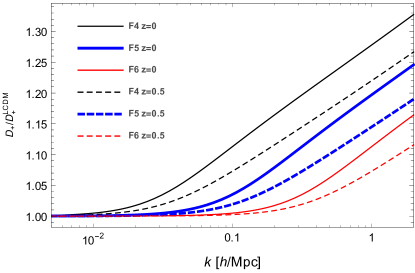
The initial time here is set to tinsubscript𝑡𝑖𝑛t_{in} and a dot means derivative with respect to the time argument. In using Eq. (50) a numerical error may arise if the function at which the operator is applied is not zero at tinsubscript𝑡𝑖𝑛t_{in}, but can be compensated if the solution is known at that time, which is the case of models with an early Einstein-de Sitter (EdS) phase, as the one we use below as an example, as well as many others found in the literature. The alternative is set tinsubscript𝑡𝑖𝑛t_{in} to be very small. For ΛΛ\LambdaCDM models there is no k𝑘k-dependence and the growth functions become DH(t)proportional-tosubscript𝐷𝐻𝑡D_{-}\propto H(t) and D+H3(t)ta3(t)H3(t)𝑑tproportional-tosubscript𝐷superscript𝐻3𝑡superscript𝑡superscript𝑎3superscript𝑡superscript𝐻3superscript𝑡differential-dsuperscript𝑡D_{+}\propto H^{3}(t)\int^{t}a^{-3}(t^{\prime})H^{-3}(t^{\prime})dt^{\prime} 1977MNRAS.179..351H ; while for the special case of EdS, D+a(t)proportional-tosubscript𝐷𝑎𝑡D_{+}\propto a(t) and Da3/2(t)proportional-tosubscript𝐷superscript𝑎32𝑡D_{-}\propto a^{-3/2}(t). In Fig. 1 we plot the ratio of MG to ΛΛ\LambdaCDM linear growth functions, this is done for the F4, F5 and F6 models, and for redshifts z=0𝑧0z=0 and z=0.5𝑧0.5z=0.5; the background cosmology is fixed with Ωm=0.281subscriptΩ𝑚0.281\Omega_{m}=0.281 and h=0.6970.697h=0.697, as given by WMAP Nine-year results 2013ApJS..208…19H .
Refer to caption
Figure 1: First order growth functions over ΛΛ\LambdaCDM growth function. We show the cases of the HS F4, F5 and F6 models and redshifts z=0𝑧0z=0 and z=0.5𝑧0.5z=0.5.

We end this section by writing the scalar field to first order,

φ(1)(k)=2A03Π(k)D+(k,t)δ0(1)(k).superscript𝜑1k2subscript𝐴03Π𝑘subscript𝐷𝑘𝑡subscriptsuperscript𝛿10k\varphi^{(1)}({\text{\bf k}})=\frac{2A_{0}}{3\Pi(k)}D_{+}(k,t)\delta^{(1)}_{0}({\text{\bf k}}). (51)

Since the factor 2A03Π(k)=2a2(A(k)A0)k22subscript𝐴03Π𝑘2superscript𝑎2𝐴𝑘subscript𝐴0superscript𝑘2\frac{2A_{0}}{3\Pi(k)}=2a^{2}\frac{(A(k)-A_{0})}{k^{2}} is smaller than unity for typical values of M1subscript𝑀1M_{1}, it follows that the scalar field perturbations evolve at a slower pace than overdensities.

IV Second order: 2LPT

In this section we compute second order quantities and develop the 2LPT theory. The frame-lagging term kernel is obtained from Eq. (38) and the first order fields given in Eqs. (48) and (51),

𝒦FL(2)(k1,k2)=2(k1k2)2k12k22(A(k1)+A(k2)2A0)+k1k2k12(A(k1)A0)+k1k2k22(A(k2)A0),subscriptsuperscript𝒦2FLsubscriptk1subscriptk22superscriptsubscriptk1subscriptk22superscriptsubscript𝑘12superscriptsubscript𝑘22𝐴subscript𝑘1𝐴subscript𝑘22subscript𝐴0subscriptk1subscriptk2superscriptsubscript𝑘12𝐴subscript𝑘1subscript𝐴0subscriptk1subscriptk2superscriptsubscript𝑘22𝐴subscript𝑘2subscript𝐴0\displaystyle\mathcal{K}^{(2)}_{\text{FL}}({\text{\bf k}}_{1},{\text{\bf k}}_{2})=2\frac{({\text{\bf k}}_{1}\cdot{\text{\bf k}}_{2})^{2}}{k_{1}^{2}k_{2}^{2}}(A(k_{1})+A(k_{2})-2A_{0})+\frac{{\text{\bf k}}_{1}\cdot{\text{\bf k}}_{2}}{k_{1}^{2}}(A(k_{1})-A_{0})+\frac{{\text{\bf k}}_{1}\cdot{\text{\bf k}}_{2}}{k_{2}^{2}}(A(k_{2})-A_{0}), (52)

while the self interacting term in Eq. (III) becomes

δI(2)(k)=12(2A03)2k12=kM2(k1,k2)D+(k1)D+(k2)Π(k1)Π(k2)δ1δ2.𝛿superscript𝐼2k12superscript2subscript𝐴032subscriptk12ksubscript𝑀2subscriptk1subscriptk2subscript𝐷subscript𝑘1subscript𝐷subscript𝑘2Πsubscript𝑘1Πsubscript𝑘2subscript𝛿1subscript𝛿2\delta I^{(2)}({\text{\bf k}})=\frac{1}{2}\left(\frac{2A_{0}}{3}\right)^{2}\underset{{\text{\bf k}}_{12}={\text{\bf k}}}{\int}M_{2}({\text{\bf k}}_{1},{\text{\bf k}}_{2})\frac{D_{+}(k_{1})D_{+}(k_{2})}{\Pi(k_{1})\Pi(k_{2})}\delta_{1}\delta_{2}. (53)

Hereafter δ1subscript𝛿1\delta_{1} and δ2subscript𝛿2\delta_{2} denote the linear density contrasts with wavenumbers k1subscriptk1{\text{\bf k}}_{1} and k2subscriptk2{\text{\bf k}}_{2} evaluated at present time.

A straightforward computation of Eq. (III), see Appendix B.1, gives the Lagrangian displacement to second order:

kiΨi(2)(k)=i2k12=k37(D¯a(2)(k1,k2)D¯b(2)(k1,k2)(k1k2)2k12k22D¯δI(2)(k1,k2)+D¯FL(2)(k1,k2))D+(k1)D+(k2)δ1δ2.subscriptk𝑖superscriptΨ𝑖2k𝑖2subscriptk12k37subscriptsuperscript¯𝐷2𝑎subscriptk1subscriptk2subscriptsuperscript¯𝐷2𝑏subscriptk1subscriptk2superscriptsubscriptk1subscriptk22superscriptsubscript𝑘12superscriptsubscript𝑘22subscriptsuperscript¯𝐷2𝛿𝐼subscriptk1subscriptk2subscriptsuperscript¯𝐷2FLsubscriptk1subscriptk2subscript𝐷subscript𝑘1subscript𝐷subscript𝑘2subscript𝛿1subscript𝛿2{\text{\bf k}}_{i}\Psi^{i(2)}({\text{\bf k}})=\frac{i}{2}\underset{{\text{\bf k}}_{12}={\text{\bf k}}}{\int}\frac{3}{7}\left(\bar{D}^{(2)}_{a}({\text{\bf k}}_{1},{\text{\bf k}}_{2})-\bar{D}^{(2)}_{b}({\text{\bf k}}_{1},{\text{\bf k}}_{2})\frac{({\text{\bf k}}_{1}\cdot{\text{\bf k}}_{2})^{2}}{k_{1}^{2}k_{2}^{2}}-\bar{D}^{(2)}_{\delta I}({\text{\bf k}}_{1},{\text{\bf k}}_{2})+\bar{D}^{(2)}_{\text{FL}}({\text{\bf k}}_{1},{\text{\bf k}}_{2})\right)D_{+}(k_{1})D_{+}(k_{2})\delta_{1}\delta_{2}. (54)

Momentum conservation implies k=k12k1+k2ksubscriptk12subscriptk1subscriptk2{\text{\bf k}}={\text{\bf k}}_{12}\equiv{\text{\bf k}}_{1}+{\text{\bf k}}_{2}, as it is explicit in the Dirac delta function. The growth functions are given by

Da(2)(k1,k2)subscriptsuperscript𝐷2𝑎subscriptk1subscriptk2\displaystyle D^{(2)}_{a}({\text{\bf k}}_{1},{\text{\bf k}}_{2}) =(𝒯^A(k))1(A(k)D+(k1)D+(k2))absentsuperscript^𝒯𝐴𝑘1𝐴𝑘subscript𝐷subscript𝑘1subscript𝐷subscript𝑘2\displaystyle=\big{(}\mathbf{\hat{\mathcal{T}}}-A(k)\big{)}^{-1}\big{(}A(k)D_{+}(k_{1})D_{+}(k_{2})\big{)} (55)
Db(2)(k1,k2)subscriptsuperscript𝐷2𝑏subscriptk1subscriptk2\displaystyle D^{(2)}_{b}({\text{\bf k}}_{1},{\text{\bf k}}_{2}) =(𝒯^A(k))1((A(k1)+A(k2)A(k))D+(k1)D+(k2)),absentsuperscript^𝒯𝐴𝑘1𝐴subscript𝑘1𝐴subscript𝑘2𝐴𝑘subscript𝐷subscript𝑘1subscript𝐷subscript𝑘2\displaystyle=\big{(}\mathbf{\hat{\mathcal{T}}}-A(k)\big{)}^{-1}\big{(}(A(k_{1})+A(k_{2})-A(k))D_{+}(k_{1})D_{+}(k_{2})\big{)}, (56)
DFL(2)(k1,k2)subscriptsuperscript𝐷2FLsubscriptk1subscriptk2\displaystyle D^{(2)}_{\text{FL}}({\text{\bf k}}_{1},{\text{\bf k}}_{2}) =(𝒯^A(k))1(M1(k)3Π(k)𝒦FL(2)(k1,k2)D+(k1)D+(k2)),absentsuperscript^𝒯𝐴𝑘1subscript𝑀1𝑘3Π𝑘subscriptsuperscript𝒦2FLsubscriptk1subscriptk2subscript𝐷subscript𝑘1subscript𝐷subscript𝑘2\displaystyle=\big{(}\mathbf{\hat{\mathcal{T}}}-A(k)\big{)}^{-1}\left(\frac{M_{1}(k)}{3\Pi(k)}\mathcal{K}^{(2)}_{\text{FL}}({\text{\bf k}}_{1},{\text{\bf k}}_{2})D_{+}(k_{1})D_{+}(k_{2})\right), (57)
DδI(2)(k1,k2)subscriptsuperscript𝐷2𝛿𝐼subscriptk1subscriptk2\displaystyle D^{(2)}_{\delta I}({\text{\bf k}}_{1},{\text{\bf k}}_{2}) =(𝒯^A(k))1((2A03)2k2a2M2(k1,k2)D+(k1)D+(k2)6Π(k)Π(k1)Π(k2)),absentsuperscript^𝒯𝐴𝑘1superscript2subscript𝐴032superscript𝑘2superscript𝑎2subscript𝑀2subscriptk1subscriptk2subscript𝐷subscript𝑘1subscript𝐷subscript𝑘26Π𝑘Πsubscript𝑘1Πsubscript𝑘2\displaystyle=\big{(}\mathbf{\hat{\mathcal{T}}}-A(k)\big{)}^{-1}\left(\left(\frac{2A_{0}}{3}\right)^{2}\frac{k^{2}}{a^{2}}\frac{M_{2}({\text{\bf k}}_{1},{\text{\bf k}}_{2})D_{+}(k_{1})D_{+}(k_{2})}{6\Pi(k)\Pi(k_{1})\Pi(k_{2})}\right), (58)

and the normalized growth functions are defined as

D¯a,b,δI,FL(2)(k1,k2,t)subscriptsuperscript¯𝐷2𝑎𝑏𝛿𝐼FLsubscriptk1subscriptk2𝑡\displaystyle\bar{D}^{(2)}_{a,b,\delta I,\text{FL}}({\text{\bf k}}_{1},{\text{\bf k}}_{2},t) =73Da,b,δI,FL(2)(k1,k2,t)D+(k1)D+(k2).absent73subscriptsuperscript𝐷2𝑎𝑏𝛿𝐼FLsubscriptk1subscriptk2𝑡subscript𝐷subscript𝑘1subscript𝐷subscript𝑘2\displaystyle=\frac{7}{3}\frac{D^{(2)}_{a,b,\delta I,\text{FL}}({\text{\bf k}}_{1},{\text{\bf k}}_{2},t)}{D_{+}(k_{1})D_{+}(k_{2})}. (59)

The growth functions depend only on three numbers, these can be chosen as k1subscript𝑘1k_{1}, k2subscript𝑘2k_{2} and k12subscript𝑘12k_{12}, such that alternatively we can write

D¯(2)(k1,k2)=D¯(2)(k12,k1,k2).superscript¯𝐷2subscriptk1subscriptk2superscript¯𝐷2subscript𝑘12subscript𝑘1subscript𝑘2\bar{D}^{(2)}({\text{\bf k}}_{1},{\text{\bf k}}_{2})=\bar{D}^{(2)}(k_{12},k_{1},k_{2}). (60)

Both notations will be used interchangeably.

The linear operator (𝒯^A(k))^𝒯𝐴𝑘(\mathbf{\hat{\mathcal{T}}}-A(k)) is not invertible over its whole domain, and (𝒯^A(k))1hsuperscript^𝒯𝐴𝑘1(\mathbf{\hat{\mathcal{T}}}-A(k))^{-1}h is only a particular solution to the differential equation (𝒯^A(k))f=h^𝒯𝐴𝑘𝑓(\mathbf{\hat{\mathcal{T}}}-A(k))f=h. The growth functions obtained from Eqs. (55)-(58) project out the linear order solution to Eq. (49), as it is required for being pure second order functions. On the other hand, numerical computations using differential equations instead, present no disadvantages if the initial conditions are carefully chosen.

For dark energy models in which we can neglect dark energy perturbations or MG scale independent models, we have I2(t)D¯a(2)(t)=D¯b(2)(t)subscript𝐼2𝑡subscriptsuperscript¯𝐷2𝑎𝑡subscriptsuperscript¯𝐷2𝑏𝑡I_{2}(t)\equiv\bar{D}^{(2)}_{a}(t)=\bar{D}^{(2)}_{b}(t) (following the notation of Lee:2014maa ), and D¯δI(2)=D¯FL(2)=0subscriptsuperscript¯𝐷2𝛿𝐼subscriptsuperscript¯𝐷2FL0\bar{D}^{(2)}_{\delta I}=\bar{D}^{(2)}_{\text{FL}}=0. For EdS, these reduce to I2(t)=1subscript𝐼2𝑡1I_{2}(t)=1, and for ΛΛ\LambdaCDM I2(t)1.01similar-to-or-equalssubscript𝐼2𝑡1.01I_{2}(t)\simeq 1.01 at the present time for Ωm00.3similar-to-or-equalssubscriptΩ𝑚00.3\Omega_{m0}\simeq 0.3.


We can write the divergence of the Lagrangian displacement as

kiΨ(2)i(k)=i2k12=kD(2)(k1,k2)δ1δ2,subscript𝑘𝑖superscriptΨ2𝑖k𝑖2subscriptk12ksuperscript𝐷2subscriptk1subscriptk2subscript𝛿1subscript𝛿2k_{i}\Psi^{(2)i}({\text{\bf k}})=\frac{i}{2}\underset{{\text{\bf k}}_{12}={\text{\bf k}}}{\int}D^{(2)}({\text{\bf k}}_{1},{\text{\bf k}}_{2})\delta_{1}\delta_{2}, (61)

with

D(2)(k1,k2)=Da(2)(k1,k2)Db(2)(k1,k2)(k1k2)2k12k22DδI(2)(k1,k2)+DFL(2)(k1,k2),superscript𝐷2subscriptk1subscriptk2subscriptsuperscript𝐷2𝑎subscriptk1subscriptk2superscriptsubscript𝐷𝑏2subscriptk1subscriptk2superscriptsubscriptk1subscriptk22superscriptsubscript𝑘12superscriptsubscript𝑘22subscriptsuperscript𝐷2𝛿𝐼subscriptk1subscriptk2subscriptsuperscript𝐷2FLsubscriptk1subscriptk2D^{(2)}({\text{\bf k}}_{1},{\text{\bf k}}_{2})=D^{(2)}_{a}({\text{\bf k}}_{1},{\text{\bf k}}_{2})-D_{b}^{(2)}({\text{\bf k}}_{1},{\text{\bf k}}_{2})\frac{({\text{\bf k}}_{1}\cdot{\text{\bf k}}_{2})^{2}}{k_{1}^{2}k_{2}^{2}}-D^{(2)}_{\delta I}({\text{\bf k}}_{1},{\text{\bf k}}_{2})+D^{(2)}_{\text{FL}}({\text{\bf k}}_{1},{\text{\bf k}}_{2}), (62)

from which we can read the extension to the LPT second order kernel as

L(2)i(k1,k2)=kik2D(2)(k1,k2)D+(k1)D+(k2).superscript𝐿2𝑖subscriptk1subscriptk2superscript𝑘𝑖superscript𝑘2superscript𝐷2subscriptk1subscriptk2subscript𝐷subscript𝑘1subscript𝐷subscript𝑘2L^{(2)i}({\text{\bf k}}_{1},{\text{\bf k}}_{2})=\frac{k^{i}}{k^{2}}\frac{D^{(2)}({\text{\bf k}}_{1},{\text{\bf k}}_{2})}{D_{+}(k_{1})D_{+}(k_{2})}. (63)

Consider now the collapse of parallel sheets of matter. In GR it is well known that the equation of motion for the Lagrangian displacement becomes linear and the Zel’dovich approximation is the exact solution. This is because the Newtonian gravitational force, which decays as the inverse of the squared distance, becomes a constant regardless the separation of the sheets McQuinn:2015tva . Therefore, the second and higher order Lagrangian displacement kernels are zero. This can be deduced from Eq. (62) by setting Da(2)=Db(2)subscriptsuperscript𝐷2𝑎subscriptsuperscript𝐷2𝑏D^{(2)}_{a}=D^{(2)}_{b}, DδI(2)=DFL(2)=0subscriptsuperscript𝐷2𝛿𝐼subscriptsuperscript𝐷2FL0D^{(2)}_{\delta I}=D^{(2)}_{\text{FL}}=0, and choosing parallel wavevectors k1k2conditionalsubscriptk1subscriptk2{\text{\bf k}}_{1}\parallel{\text{\bf k}}_{2}, in this situation DGR(2)(k1,k2)=0subscriptsuperscript𝐷2GRsubscriptk1subscriptk20D^{(2)}_{\text{GR}}({\text{\bf k}}_{1},{\text{\bf k}}_{2})=0, as required. In modified theories of gravity the situation is rather different, the fifth force between the sheets is not longer a constant, and the growth function D(2)(k1,k2)superscript𝐷2subscriptk1subscriptk2D^{(2)}({\text{\bf k}}_{1},{\text{\bf k}}_{2}) does not vanish since Da(2)(k1,k2)Db(2)(k1,k2)subscriptsuperscript𝐷2𝑎subscriptk1subscriptk2subscriptsuperscript𝐷2𝑏subscriptk1subscriptk2D^{(2)}_{a}({\text{\bf k}}_{1},{\text{\bf k}}_{2})\neq D^{(2)}_{b}({\text{\bf k}}_{1},{\text{\bf k}}_{2}). Nevertheless, at the scales the fifth force can be neglected we have to recover the GR result, this should be the case in the large scales limit of k0𝑘0k\rightarrow 0. Since Da(2)(k=0,k1,k2)Db(2)(k=0,k1,k2)superscriptsubscript𝐷𝑎2𝑘0subscript𝑘1subscript𝑘2superscriptsubscript𝐷𝑏2𝑘0subscript𝑘1subscript𝑘2D_{a}^{(2)}(k=0,k_{1},k_{2})\neq D_{b}^{(2)}(k=0,k_{1},k_{2}) and DδI(2)(k=0,k1,k2)=0subscriptsuperscript𝐷2𝛿𝐼𝑘0subscript𝑘1subscript𝑘20D^{(2)}_{\delta I}(k=0,k_{1},k_{2})=0, the cancellation should be accomplished by the frame-lagging. Indeed, the squeezed configuration of triangles formed as k=k1+k2ksubscriptk1subscriptk2{\text{\bf k}}={\text{\bf k}}_{1}+{\text{\bf k}}_{2} with k120similar-to-or-equalssubscriptk120{\text{\bf k}}_{12}\simeq 0, k1psimilar-to-or-equalssubscriptk1p{\text{\bf k}}_{1}\simeq{\text{\bf p}} and k2psimilar-to-or-equalssubscriptk2p{\text{\bf k}}_{2}\simeq-{\text{\bf p}} is a planar collapse; and, by using Eqs. (52),(55)-(58),(62), and the identity M1(0)=3Π(0)subscript𝑀103Π0M_{1}(0)=3\Pi(0), it is easy to see that D(2)(p,p)=0superscript𝐷2pp0D^{(2)}({\text{\bf p}},-{\text{\bf p}})=0, recovering GR when k2/a2M1much-less-thansuperscript𝑘2superscript𝑎2subscript𝑀1k^{2}/a^{2}\ll M_{1}.

As it was mentioned in the Introduction, 2LPT equations in MG have been derived in two (to our knowledge) separate works Valogiannis:2016ane ; Winther:2017jof . In Valogiannis:2016ane the results differ with the given here, since the authors find Da(2)=Db(2)superscriptsubscript𝐷𝑎2superscriptsubscript𝐷𝑏2D_{a}^{(2)}=D_{b}^{(2)} and, furthermore, they do not seem to consider the frame-lagging. In Winther:2017jof their computations to second order coincide with ours. In those works the authors use 2LPT for implementations of MG into the COLA code, obtaining very satisfactory results. These works share the ΛΛ\LambdaCDM as a limit at large scales, where the 2LPT in COLA implementations is more important. Indeed, to speed-up computations, in Ref. Valogiannis:2016ane the 2LPT of ΛΛ\LambdaCDM is additionally used into the MG runs, finding also a good agreement with N𝑁N-body simulations.

Refer to caption
Refer to caption
Refer to caption
Refer to caption
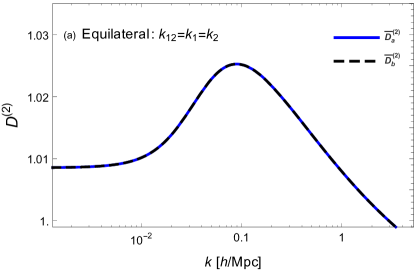
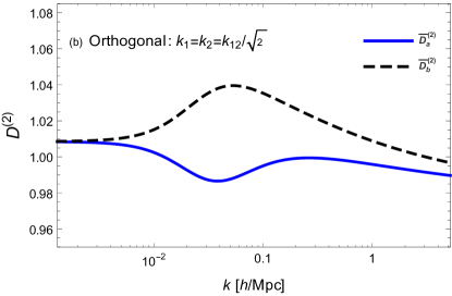
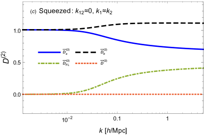
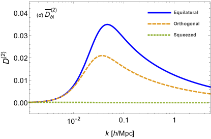
Figure 2: Second order normalized growth functions D¯a(2)subscriptsuperscript¯𝐷2𝑎\bar{D}^{(2)}_{a}, D¯b(2)subscriptsuperscript¯𝐷2𝑏\bar{D}^{(2)}_{b},D¯δI(2)subscriptsuperscript¯𝐷2𝛿𝐼\bar{D}^{(2)}_{\delta I} and D¯FL(2)subscriptsuperscript¯𝐷2FL\bar{D}^{(2)}_{\text{FL}}, for the F4 model. Different triangular configurations are considered. See text for details.

In Fig.2 we plot second order growth functions for the F4 case444The effects of F5, and F6 are qualitatively very similar but are shifted toward higher values of k𝑘k. and we choose three different triangular configurations: (a) equilateral for which k12=k1=k2subscript𝑘12subscript𝑘1subscript𝑘2k_{12}=k_{1}=k_{2}; (b) orthogonal with k12=2k1=2k2subscript𝑘122subscript𝑘12subscript𝑘2k_{12}=\sqrt{2}k_{1}=\sqrt{2}k_{2}; and (c) squeezed, k120similar-to-or-equalssubscript𝑘120k_{12}\simeq 0, k1k2similar-to-or-equalssubscript𝑘1subscript𝑘2k_{1}\simeq k_{2}. We can read from the equations for the growth functions that in the case of equilateral configuration we have D¯a(2)=D¯b(2)superscriptsubscript¯𝐷𝑎2superscriptsubscript¯𝐷𝑏2\bar{D}_{a}^{(2)}=\bar{D}_{b}^{(2)}. The squeezed case corresponds to the limit of large scales where the theory reduces to ΛΛ\LambdaCDM, we can see from panel (c) in Fig. 2 that actually by considering the combination D¯a(2)D¯b(2)+D¯FL(2)subscriptsuperscript¯𝐷2𝑎subscriptsuperscript¯𝐷2𝑏subscriptsuperscript¯𝐷2FL\bar{D}^{(2)}_{a}-\bar{D}^{(2)}_{b}+\bar{D}^{(2)}_{\text{FL}} (dotted red line in panel (c)) in this configuration we get D(2)=0superscript𝐷20D^{(2)}=0, as was shown analytically above. The frame-lagging second order growth function for equilateral configuration is exactly zero and for the orthogonal is very similar in shape to the squeezed one, but reaching smaller values. In panel (d) we show the screening normalized growth functions for the three considered triangular configurations. We make note that the functions D¯a(2)superscriptsubscript¯𝐷𝑎2\bar{D}_{a}^{(2)} and D¯b(2)superscriptsubscript¯𝐷𝑏2\bar{D}_{b}^{(2)} do not tend to 1 as k𝑘k goes to zero, the EdS value, instead their limits are 1.009similar-toabsent1.009\sim 1.009, the I2(t0)subscript𝐼2subscript𝑡0I_{2}(t_{0}) value for the chosen cosmological parameters in the ΛΛ\LambdaCDM model.


Now, we calculate the matter and scalar field perturbation to second order. From Eq. (46), δ~(2)(k)=[Ψi,i(2)+12(Ψi,i(1)Ψj,j(1)+Ψi,j(1)Ψj,i(1))](k)superscript~𝛿2kdelimited-[]superscriptsubscriptΨ𝑖𝑖212superscriptsubscriptΨ𝑖𝑖1superscriptsubscriptΨ𝑗𝑗1superscriptsubscriptΨ𝑖𝑗1superscriptsubscriptΨ𝑗𝑖1k\tilde{\delta}^{(2)}({\text{\bf k}})=[-\Psi_{i,i}^{(2)}+\frac{1}{2}(\Psi_{i,i}^{(1)}\Psi_{j,j}^{(1)}+\Psi_{i,j}^{(1)}\Psi_{j,i}^{(1)})]({\text{\bf k}}), then

δ~(2)(k)=12k12=k(D(2)(k1,k2)+(1+(k1k2)2k12k22)D+(k1)D+(k2))δ1δ2,superscript~𝛿2k12subscriptk12ksuperscript𝐷2subscriptk1subscriptk21superscriptsubscriptk1subscriptk22superscriptsubscript𝑘12superscriptsubscript𝑘22subscript𝐷subscript𝑘1subscript𝐷subscript𝑘2subscript𝛿1subscript𝛿2\tilde{\delta}^{(2)}({\text{\bf k}})=\frac{1}{2}\underset{{\text{\bf k}}_{12}={\text{\bf k}}}{\int}\left(D^{(2)}({\text{\bf k}}_{1},{\text{\bf k}}_{2})+\left(1+\frac{({\text{\bf k}}_{1}\cdot{\text{\bf k}}_{2})^{2}}{k_{1}^{2}k_{2}^{2}}\right)D_{+}(k_{1})D_{+}(k_{2})\right)\delta_{1}\delta_{2}, (64)

and the scalar field becomes

φ(2)(k)=2A03Π(k)12k12=kDφ(2)(k1,k2)δ1δ2,superscript𝜑2k2subscript𝐴03Π𝑘12subscriptk12ksubscriptsuperscript𝐷2𝜑subscriptk1subscriptk2subscript𝛿1subscript𝛿2\varphi^{(2)}({\text{\bf k}})=\frac{2A_{0}}{3\Pi(k)}\frac{1}{2}\underset{{\text{\bf k}}_{12}={\text{\bf k}}}{\int}D^{(2)}_{\varphi}({\text{\bf k}}_{1},{\text{\bf k}}_{2})\delta_{1}\delta_{2}, (65)

with

Dφ(2)(k1,k2)subscriptsuperscript𝐷2𝜑subscriptk1subscriptk2\displaystyle D^{(2)}_{\varphi}({\text{\bf k}}_{1},{\text{\bf k}}_{2}) =D(2)(k1,k2)+(1+(k1k2)2k12k22)D+(k1)D+(k2)absentsuperscript𝐷2subscriptk1subscriptk21superscriptsubscriptk1subscriptk22superscriptsubscript𝑘12superscriptsubscript𝑘22subscript𝐷subscript𝑘1subscript𝐷subscript𝑘2\displaystyle=D^{(2)}({\text{\bf k}}_{1},{\text{\bf k}}_{2})+\left(1+\frac{({\text{\bf k}}_{1}\cdot{\text{\bf k}}_{2})^{2}}{k_{1}^{2}k_{2}^{2}}\right)D_{+}(k_{1})D_{+}(k_{2})
2A03M2(k1,k2)+JFL(k1,k2)(3+2ωBD)3Π(k1)Π(k2)D+(k1)D+(k2).2subscript𝐴03subscript𝑀2subscriptk1subscriptk2subscript𝐽FLsubscriptk1subscriptk232subscript𝜔BD3Πsubscript𝑘1Πsubscript𝑘2subscript𝐷subscript𝑘1subscript𝐷subscript𝑘2\displaystyle-\frac{2A_{0}}{3}\frac{M_{2}({\text{\bf k}}_{1},{\text{\bf k}}_{2})+J_{\text{FL}}({\text{\bf k}}_{1},{\text{\bf k}}_{2})(3+2\omega_{\text{BD}})}{3\Pi(k_{1})\Pi(k_{2})}D_{+}(k_{1})D_{+}(k_{2}). (66)

We shall use the above perturbations in the following section to find the third order Lagrangian displacement field.

V Third order

In this section we compute the expansion of the relevant fields up to third order. Using Eqs. (38), (61) and (65), the frame-lagging kernel is

𝒦FL(3)(k1,k2,k3)subscriptsuperscript𝒦3FLsubscriptk1subscriptk2subscriptk3\displaystyle\mathcal{K}^{(3)}_{\text{FL}}({\text{\bf k}}_{1},{\text{\bf k}}_{2},{\text{\bf k}}_{3}) =3(2(k1k23)2k12k232+k1k23k12)D(2)(k2,k3)D+(k2)D+(k3)(A(k1)A0)absent32superscriptsubscriptk1subscriptk232superscriptsubscript𝑘12superscriptsubscript𝑘232subscriptk1subscriptk23superscriptsubscript𝑘12superscript𝐷2subscriptk2subscriptk3subscript𝐷subscript𝑘2subscript𝐷subscript𝑘3𝐴subscript𝑘1subscript𝐴0\displaystyle=3\left(2\frac{({\text{\bf k}}_{1}\cdot{\text{\bf k}}_{23})^{2}}{k_{1}^{2}k_{23}^{2}}+\frac{{\text{\bf k}}_{1}\cdot{\text{\bf k}}_{23}}{k_{1}^{2}}\right)\frac{D^{(2)}({\text{\bf k}}_{2},{\text{\bf k}}_{3})}{D_{+}(k_{2})D_{+}(k_{3})}(A(k_{1})-A_{0})
+3(2(k1k23)2k12k232+k1k23k232)Dφ(2)(k2,k3)D+(k2)D+(k3)(A(k23)A0)32superscriptsubscriptk1subscriptk232superscriptsubscript𝑘12superscriptsubscript𝑘232subscriptk1subscriptk23superscriptsubscript𝑘232subscriptsuperscript𝐷2𝜑subscriptk2subscriptk3subscript𝐷subscript𝑘2subscript𝐷subscript𝑘3𝐴subscript𝑘23subscript𝐴0\displaystyle+3\left(2\frac{({\text{\bf k}}_{1}\cdot{\text{\bf k}}_{23})^{2}}{k_{1}^{2}k_{23}^{2}}+\frac{{\text{\bf k}}_{1}\cdot{\text{\bf k}}_{23}}{k_{23}^{2}}\right)\frac{D^{(2)}_{\varphi}({\text{\bf k}}_{2},{\text{\bf k}}_{3})}{D_{+}(k_{2})D_{+}(k_{3})}(A(k_{23})-A_{0})
+6(3(k1k2)(k2k3)(k3k1)k22k32k12+2(k2k3)2(k3k1)k22k32k12+(k2k3)(k3k1)k32k12)(A(k1)A0).63subscriptk1subscriptk2subscriptk2subscriptk3subscriptk3subscriptk1superscriptsubscript𝑘22superscriptsubscript𝑘32superscriptsubscript𝑘122superscriptsubscriptk2subscriptk32subscriptk3subscriptk1superscriptsubscript𝑘22superscriptsubscript𝑘32superscriptsubscript𝑘12subscriptk2subscriptk3subscriptk3subscriptk1superscriptsubscript𝑘32superscriptsubscript𝑘12𝐴subscript𝑘1subscript𝐴0\displaystyle+6\left(3\frac{({\text{\bf k}}_{1}\cdot{\text{\bf k}}_{2})({\text{\bf k}}_{2}\cdot{\text{\bf k}}_{3})({\text{\bf k}}_{3}\cdot{\text{\bf k}}_{1})}{k_{2}^{2}k_{3}^{2}k_{1}^{2}}+2\frac{({\text{\bf k}}_{2}\cdot{\text{\bf k}}_{3})^{2}({\text{\bf k}}_{3}\cdot{\text{\bf k}}_{1})}{k_{2}^{2}k_{3}^{2}k_{1}^{2}}+\frac{({\text{\bf k}}_{2}\cdot{\text{\bf k}}_{3})({\text{\bf k}}_{3}\cdot{\text{\bf k}}_{1})}{k_{3}^{2}k_{1}^{2}}\right)(A(k_{1})-A_{0}). (67)

The third order screening gives

δI(3)=16k123=k𝒦δI(3)(k1,k2,k3)D+(k1)D+(k2)D+(k3)δ1δ2δ3,𝛿superscript𝐼316subscriptk123ksubscriptsuperscript𝒦3𝛿𝐼subscriptk1subscriptk2subscriptk3subscript𝐷subscript𝑘1subscript𝐷subscript𝑘2subscript𝐷subscript𝑘3subscript𝛿1subscript𝛿2subscript𝛿3\delta I^{(3)}=\frac{1}{6}\underset{{\text{\bf k}}_{123}={\text{\bf k}}}{\int}\mathcal{K}^{(3)}_{\delta I}({\text{\bf k}}_{1},{\text{\bf k}}_{2},{\text{\bf k}}_{3})D_{+}(k_{1})D_{+}(k_{2})D_{+}(k_{3})\delta_{1}\delta_{2}\delta_{3}, (68)

with kernel

𝒦δI(3)(k1,k2,k3)subscriptsuperscript𝒦3𝛿𝐼subscriptk1subscriptk2subscriptk3\displaystyle\mathcal{K}^{(3)}_{\delta I}({\text{\bf k}}_{1},{\text{\bf k}}_{2},{\text{\bf k}}_{3}) =(2A03)23M2(k1,k23)Π(k1)Π(k23)(1+(k2k2)2k22k32+D(2)(k2,k3)D+(k2)D+(k3))absentsuperscript2subscript𝐴0323subscript𝑀2subscriptk1subscriptk23Πsubscript𝑘1Πsubscript𝑘231superscriptsubscriptk2subscriptk22superscriptsubscript𝑘22superscriptsubscript𝑘32superscript𝐷2subscriptk2subscriptk3subscript𝐷subscript𝑘2subscript𝐷subscript𝑘3\displaystyle=\left(\frac{2A_{0}}{3}\right)^{2}\frac{3M_{2}({\text{\bf k}}_{1},{\text{\bf k}}_{23})}{\Pi(k_{1})\Pi(k_{23})}\left(1+\frac{({\text{\bf k}}_{2}\cdot{\text{\bf k}}_{2})^{2}}{k_{2}^{2}k_{3}^{2}}+\frac{D^{(2)}({\text{\bf k}}_{2},{\text{\bf k}}_{3})}{D_{+}(k_{2})D_{+}(k_{3})}\right)
+(2A03)3(M3(k1,k2,k3)Π(k1)Π(k2)Π(k3)M2(k1,k23)(M2(k2,k3)+JFL(2)(k2,k3)(3+2wBD))Π(k23)Π(k1)Π(k2)Π(k3)).superscript2subscript𝐴033subscript𝑀3subscript𝑘1subscript𝑘2subscript𝑘3Πsubscript𝑘1Πsubscript𝑘2Πsubscript𝑘3subscript𝑀2subscriptk1subscriptk23subscript𝑀2subscriptk2subscriptk3subscriptsuperscript𝐽2𝐹𝐿subscriptk2subscriptk332subscript𝑤BDΠsubscript𝑘23Πsubscript𝑘1Πsubscript𝑘2Πsubscript𝑘3\displaystyle+\left(\frac{2A_{0}}{3}\right)^{3}\left(\frac{M_{3}(k_{1},k_{2},k_{3})}{\Pi(k_{1})\Pi(k_{2})\Pi(k_{3})}-\frac{M_{2}({\text{\bf k}}_{1},{\text{\bf k}}_{23})(M_{2}({\text{\bf k}}_{2},{\text{\bf k}}_{3})+J^{(2)}_{FL}({\text{\bf k}}_{2},{\text{\bf k}}_{3})(3+2w_{\text{BD}}))}{\Pi(k_{23})\Pi(k_{1})\Pi(k_{2})\Pi(k_{3})}\right). (69)

A straightforward but lengthy computation, see Appendix B.2, leads to

kiΨ(3)i(k)subscript𝑘𝑖superscriptΨ3𝑖k\displaystyle k_{i}\Psi^{(3)i}({\text{\bf k}}) =i6k123=kD+(k1)D+(k2)D+(k3)δ1δ2δ3{57(D¯A(3)D¯B(3)(k2k3)2k22k23+D¯CTa(3))(1(k1k23)2k12k232)\displaystyle=\frac{i}{6}\underset{{\text{\bf k}}_{123}={\text{\bf k}}}{\int}D_{+}(k_{1})D_{+}(k_{2})D_{+}(k_{3})\delta_{1}\delta_{2}\delta_{3}\Bigg{\{}\frac{5}{7}\left(\bar{D}^{(3)}_{A}-\bar{D}^{(3)}_{B}\frac{({\text{\bf k}}_{2}\cdot{\text{\bf k}}_{3})^{2}}{k^{2}_{2}k^{3}_{2}}+\bar{D}^{(3)}_{CTa}\right)\left(1-\frac{({\text{\bf k}}_{1}\cdot{\text{\bf k}}_{23})^{2}}{k_{1}^{2}k_{23}^{2}}\right)
13(D¯C(3)3D¯D(3)(k2k3)2k22k23+2D¯E(3)(k1k2)(k2k3)(k3k1)k12k22k32+D¯CTb(3))D¯δI(3)+D¯FL(3)},\displaystyle\quad\qquad-\frac{1}{3}\left(\,\bar{D}^{(3)}_{C}-3\bar{D}^{(3)}_{D}\frac{({\text{\bf k}}_{2}\cdot{\text{\bf k}}_{3})^{2}}{k^{2}_{2}k^{3}_{2}}+2\bar{D}^{(3)}_{E}\frac{({\text{\bf k}}_{1}\cdot{\text{\bf k}}_{2})({\text{\bf k}}_{2}\cdot{\text{\bf k}}_{3})({\text{\bf k}}_{3}\cdot{\text{\bf k}}_{1})}{k_{1}^{2}k^{2}_{2}k^{2}_{3}}+\bar{D}^{(3)}_{CTb}\,\right)-\bar{D}^{(3)}_{\delta I}+\bar{D}^{(3)}_{\text{FL}}\Bigg{\}}, (70)

with normalized growth functions

D¯A,B,CTa(3)(k1,k2,k3)subscriptsuperscript¯𝐷3𝐴𝐵𝐶𝑇𝑎subscriptk1subscriptk2subscriptk3\displaystyle\bar{D}^{(3)}_{A,B,CTa}({\text{\bf k}}_{1},{\text{\bf k}}_{2},{\text{\bf k}}_{3}) =75DA,B,CTa(3)(k1,k2,k3)D+(k1)D+(k2)D+(k3),absent75subscriptsuperscript𝐷3𝐴𝐵𝐶𝑇𝑎subscriptk1subscriptk2subscriptk3subscript𝐷subscript𝑘1subscript𝐷subscript𝑘2subscript𝐷subscript𝑘3\displaystyle=\frac{7}{5}\frac{D^{(3)}_{A,B,CTa}({\text{\bf k}}_{1},{\text{\bf k}}_{2},{\text{\bf k}}_{3})}{D_{+}(k_{1})D_{+}(k_{2})D_{+}(k_{3})}, (71)
D¯C,D,E,δI,FL,CTb(3)(k1,k2,k3)subscriptsuperscript¯𝐷3𝐶𝐷𝐸𝛿𝐼FL𝐶𝑇𝑏subscriptk1subscriptk2subscriptk3\displaystyle\bar{D}^{(3)}_{C,D,E,\delta I,\text{FL},CTb}({\text{\bf k}}_{1},{\text{\bf k}}_{2},{\text{\bf k}}_{3}) =DC,D,E,δI,FL,CTb(3)(k1,k2,k3)D+(k1)D+(k2)D+(k3),absentsubscriptsuperscript𝐷3𝐶𝐷𝐸𝛿𝐼FL𝐶𝑇𝑏subscriptk1subscriptk2subscriptk3subscript𝐷subscript𝑘1subscript𝐷subscript𝑘2subscript𝐷subscript𝑘3\displaystyle=\frac{D^{(3)}_{C,D,E,\delta I,\text{FL},CTb}({\text{\bf k}}_{1},{\text{\bf k}}_{2},{\text{\bf k}}_{3})}{D_{+}(k_{1})D_{+}(k_{2})D_{+}(k_{3})}, (72)

and growth functions

DA(3)subscriptsuperscript𝐷3𝐴\displaystyle D^{(3)}_{A} =(𝒯^A(k))1(3D+(k1)(A(k1)+𝒯^A(k))Da(2)(k2,k3)),absentsuperscript^𝒯𝐴𝑘13subscript𝐷subscript𝑘1𝐴subscript𝑘1^𝒯𝐴𝑘subscriptsuperscript𝐷2𝑎subscriptk2subscriptk3\displaystyle=\left(\mathbf{\hat{\mathcal{T}}}-A(k)\right)^{-1}\left(3D_{+}(k_{1})\big{(}A(k_{1})+\mathbf{\hat{\mathcal{T}}}-A(k)\big{)}D^{(2)}_{a}({\text{\bf k}}_{2},{\text{\bf k}}_{3})\right), (73)
DB(3)subscriptsuperscript𝐷3𝐵\displaystyle D^{(3)}_{B} =(𝒯^A(k))1(3D+(k1)(A(k1)+𝒯^A(k))Db(2)(k2,k3)),absentsuperscript^𝒯𝐴𝑘13subscript𝐷subscript𝑘1𝐴subscript𝑘1^𝒯𝐴𝑘subscriptsuperscript𝐷2𝑏subscriptk2subscriptk3\displaystyle=\left(\mathbf{\hat{\mathcal{T}}}-A(k)\right)^{-1}\left(3D_{+}(k_{1})\big{(}A(k_{1})+\mathbf{\hat{\mathcal{T}}}-A(k)\big{)}D^{(2)}_{b}({\text{\bf k}}_{2},{\text{\bf k}}_{3})\right), (74)
DCTa(3)subscriptsuperscript𝐷3𝐶𝑇𝑎\displaystyle D^{(3)}_{CTa} =(𝒯^A(k))1(3D+(k1)(A(k1)+𝒯^A(k))(DFL(2)(k2,k3)DδI(2)(k2,k3))),absentsuperscript^𝒯𝐴𝑘13subscript𝐷subscript𝑘1𝐴subscript𝑘1^𝒯𝐴𝑘subscriptsuperscript𝐷2FLsubscriptk2subscriptk3subscriptsuperscript𝐷2𝛿𝐼subscriptk2subscriptk3\displaystyle=\left(\mathbf{\hat{\mathcal{T}}}-A(k)\right)^{-1}\left(3D_{+}(k_{1})\big{(}A(k_{1})+\mathbf{\hat{\mathcal{T}}}-A(k)\big{)}\big{(}D^{(2)}_{\text{FL}}({\text{\bf k}}_{2},{\text{\bf k}}_{3})-D^{(2)}_{\delta I}({\text{\bf k}}_{2},{\text{\bf k}}_{3})\big{)}\right), (75)
DC(3)subscriptsuperscript𝐷3𝐶\displaystyle D^{(3)}_{C} =(𝒯^A(k))1(9D+(k1)(A(k1)+𝒯^2A(k))Da(2)(k2,k3)3A(k)D+(k1)D+(k2)D+(k3)),absentsuperscript^𝒯𝐴𝑘19subscript𝐷subscript𝑘1𝐴subscript𝑘1^𝒯2𝐴𝑘subscriptsuperscript𝐷2𝑎subscriptk2subscriptk33𝐴𝑘subscript𝐷subscript𝑘1subscript𝐷subscript𝑘2subscript𝐷subscript𝑘3\displaystyle=\left(\mathbf{\hat{\mathcal{T}}}-A(k)\right)^{-1}\left(9D_{+}(k_{1})\big{(}A(k_{1})+\mathbf{\hat{\mathcal{T}}}-2A(k)\big{)}D^{(2)}_{a}({\text{\bf k}}_{2},{\text{\bf k}}_{3})-3A(k)D_{+}(k_{1})D_{+}(k_{2})D_{+}(k_{3})\right), (76)
DD(3)subscriptsuperscript𝐷3𝐷\displaystyle D^{(3)}_{D} =(𝒯^A(k))1(3D+(k1)(A(k1)+𝒯^2A(k))Db(2)(k2,k3)+3A(k)D+(k1)D+(k2)D+(k3)),absentsuperscript^𝒯𝐴𝑘13subscript𝐷subscript𝑘1𝐴subscript𝑘1^𝒯2𝐴𝑘subscriptsuperscript𝐷2𝑏subscriptk2subscriptk33𝐴𝑘subscript𝐷subscript𝑘1subscript𝐷subscript𝑘2subscript𝐷subscript𝑘3\displaystyle=\left(\mathbf{\hat{\mathcal{T}}}-A(k)\right)^{-1}\left(3D_{+}(k_{1})\big{(}A(k_{1})+\mathbf{\hat{\mathcal{T}}}-2A(k)\big{)}D^{(2)}_{b}({\text{\bf k}}_{2},{\text{\bf k}}_{3})+3A(k)D_{+}(k_{1})D_{+}(k_{2})D_{+}(k_{3})\right), (77)
DE(3)subscriptsuperscript𝐷3𝐸\displaystyle D^{(3)}_{E} =(𝒯^A(k))1(3(3A(k1)A(k))D+(k1)D+(k2)D+(k3)),absentsuperscript^𝒯𝐴𝑘133𝐴subscript𝑘1𝐴𝑘subscript𝐷subscript𝑘1subscript𝐷subscript𝑘2subscript𝐷subscript𝑘3\displaystyle=\left(\mathbf{\hat{\mathcal{T}}}-A(k)\right)^{-1}\Big{(}3\big{(}3A(k_{1})-A(k)\big{)}D_{+}(k_{1})D_{+}(k_{2})D_{+}(k_{3})\Big{)}, (78)
DCTb(3)subscriptsuperscript𝐷3𝐶𝑇𝑏\displaystyle D^{(3)}_{CTb} =(𝒯^A(k))1(9D+(k1)(A(k1)+𝒯^2A(k))(DFL(2)(k2,k3)DδI(2)(k2,k3))),absentsuperscript^𝒯𝐴𝑘19subscript𝐷subscript𝑘1𝐴subscript𝑘1^𝒯2𝐴𝑘subscriptsuperscript𝐷2FLsubscriptk2subscriptk3subscriptsuperscript𝐷2𝛿𝐼subscriptk2subscriptk3\displaystyle=\left(\mathbf{\hat{\mathcal{T}}}-A(k)\right)^{-1}\left(9D_{+}(k_{1})\big{(}A(k_{1})+\mathbf{\hat{\mathcal{T}}}-2A(k)\big{)}\big{(}D^{(2)}_{\text{FL}}({\text{\bf k}}_{2},{\text{\bf k}}_{3})-D^{(2)}_{\delta I}({\text{\bf k}}_{2},{\text{\bf k}}_{3})\big{)}\right), (79)
DδI(3)subscriptsuperscript𝐷3𝛿𝐼\displaystyle D^{(3)}_{\delta I} =(𝒯^A(k))1(k2/a26Π(k)𝒦δI(3)(k1,k2,k3)D+(k1)D+(k2)D+(k3)),absentsuperscript^𝒯𝐴𝑘1superscript𝑘2superscript𝑎26Π𝑘subscriptsuperscript𝒦3𝛿𝐼subscriptk1subscriptk2subscriptk3subscript𝐷subscript𝑘1subscript𝐷subscript𝑘2subscript𝐷subscript𝑘3\displaystyle=\left(\mathbf{\hat{\mathcal{T}}}-A(k)\right)^{-1}\left(\frac{k^{2}/a^{2}}{6\Pi(k)}\mathcal{K}^{(3)}_{\delta I}({\text{\bf k}}_{1},{\text{\bf k}}_{2},{\text{\bf k}}_{3})D_{+}(k_{1})D_{+}(k_{2})D_{+}(k_{3})\right), (80)
DFL(3)subscriptsuperscript𝐷3FL\displaystyle D^{(3)}_{\text{FL}} =(𝒯^A(k))1(M13Π(k)𝒦FL(3)(k1,k2,k3)D+(k1)D+(k2)D+(k3)).absentsuperscript^𝒯𝐴𝑘1subscript𝑀13Π𝑘subscriptsuperscript𝒦3FLsubscriptk1subscriptk2subscriptk3subscript𝐷subscript𝑘1subscript𝐷subscript𝑘2subscript𝐷subscript𝑘3\displaystyle=\left(\mathbf{\hat{\mathcal{T}}}-A(k)\right)^{-1}\left(\frac{M_{1}}{3\Pi(k)}\mathcal{K}^{(3)}_{\text{FL}}({\text{\bf k}}_{1},{\text{\bf k}}_{2},{\text{\bf k}}_{3})D_{+}(k_{1})D_{+}(k_{2})D_{+}(k_{3})\right). (81)

The growth functions depend on three wavevectors, but these are constrained to form a quadrilateral k=k1+k2+k3ksubscriptk1subscriptk2subscriptk3{\text{\bf k}}={\text{\bf k}}_{1}+{\text{\bf k}}_{2}+{\text{\bf k}}_{3}; thus, they depend only on 6 numbers for a given k. Furthermore, the relevant configurations for these quadrilaterals in 2-point statistics are the so-called double squeezed in which k=k1ksubscriptk1{\text{\bf k}}=-{\text{\bf k}}_{1} and pk3=k2psubscriptk3subscriptk2{\text{\bf p}}\equiv{\text{\bf k}}_{3}=-{\text{\bf k}}_{2}, which left us with only 3 degrees of freedom, highly simplifying the analysis.

For the ΛΛ\LambdaCDM model we have DA(3)=DB(3)=(𝒯^A0)1(97D+𝒯^D+2)subscriptsuperscript𝐷3𝐴subscriptsuperscript𝐷3𝐵superscript^𝒯subscript𝐴0197subscript𝐷^𝒯superscriptsubscript𝐷2D^{(3)}_{A}=D^{(3)}_{B}=(\mathbf{\hat{\mathcal{T}}}-A_{0})^{-1}(\frac{9}{7}D_{+}\mathbf{\hat{\mathcal{T}}}D_{+}^{2}), and since 𝒯^D+2=2D+𝒯^D++2D˙+2^𝒯superscriptsubscript𝐷22subscript𝐷^𝒯subscript𝐷2superscriptsubscript˙𝐷2\mathbf{\hat{\mathcal{T}}}D_{+}^{2}=2D_{+}\mathbf{\hat{\mathcal{T}}}D_{+}+2\dot{D}_{+}^{2}, we get DA,B(3)=576(𝒯^A0)1(32ΩmH2D+3(35+25f2/Ωm))subscriptsuperscript𝐷3𝐴𝐵576superscript^𝒯subscript𝐴0132subscriptΩ𝑚superscript𝐻2superscriptsubscript𝐷33525superscript𝑓2subscriptΩ𝑚D^{(3)}_{A,B}=\frac{5}{7}6(\mathbf{\hat{\mathcal{T}}}-A_{0})^{-1}(\frac{3}{2}\Omega_{m}H^{2}D_{+}^{3}(\frac{3}{5}+\frac{2}{5}f^{2}/\Omega_{m})), with f=dlnδL/dlna𝑓𝑑subscript𝛿𝐿𝑑𝑎f=d\ln\delta_{L}/d\ln a the growth factor of linear matter perturbations. For f=Ωm1/2𝑓superscriptsubscriptΩ𝑚12f=\Omega_{m}^{1/2} we obtain the result for EdS, DA,B(3)=57D+3subscriptsuperscript𝐷3𝐴𝐵57superscriptsubscript𝐷3D^{(3)}_{A,B}=\frac{5}{7}D_{+}^{3}, meaning that the normalized growth functions D¯A,B(3)subscriptsuperscript¯𝐷3𝐴𝐵\bar{D}^{(3)}_{A,B} are exactly 1. While for ΛΛ\LambdaCDM we get D¯A,B(3)(t0)1.02similar-to-or-equalssubscriptsuperscript¯𝐷3𝐴𝐵subscript𝑡01.02\bar{D}^{(3)}_{A,B}(t_{0})\simeq 1.02 for Ωm00.3similar-to-or-equalssubscriptΩ𝑚00.3\Omega_{m0}\simeq 0.3. Analogously, we obtain DC,D,E(3)=6(𝒯^A0)1(32ΩmH2D+3)subscriptsuperscript𝐷3𝐶𝐷𝐸6superscript^𝒯subscript𝐴0132subscriptΩ𝑚superscript𝐻2superscriptsubscript𝐷3D^{(3)}_{C,D,E}=6(\mathbf{\hat{\mathcal{T}}}-A_{0})^{-1}(\frac{3}{2}\Omega_{m}H^{2}D_{+}^{3}), which reduces to DC,D,E(3)=D+3subscriptsuperscript𝐷3𝐶𝐷𝐸superscriptsubscript𝐷3D^{(3)}_{C,D,E}=D_{+}^{3} for EdS, while for ΛΛ\LambdaCDM we find D¯C,D,E(3)1.02similar-to-or-equalssubscriptsuperscript¯𝐷3𝐶𝐷𝐸1.02\bar{D}^{(3)}_{C,D,E}\simeq 1.02 at the present time. This analysis shows that the third order displacement field given by Eq. (V) reduces to the standard case when the theory is scale independent.

We can write the third order Lagrangian displacement kernel as

L(3)i(k1,k2,k3)=ikik2D(3)(k1,k2,k3)D+(k1)D+(k2)D+(k3),superscript𝐿3𝑖subscriptk1subscriptk2subscriptk3𝑖superscript𝑘𝑖superscript𝑘2superscript𝐷3subscriptk1subscriptk2subscriptk3subscript𝐷subscript𝑘1subscript𝐷subscript𝑘2subscript𝐷subscript𝑘3L^{(3)i}({\text{\bf k}}_{1},{\text{\bf k}}_{2},{\text{\bf k}}_{3})=i\frac{k^{i}}{k^{2}}\frac{D^{(3)}({\text{\bf k}}_{1},{\text{\bf k}}_{2},{\text{\bf k}}_{3})}{D_{+}(k_{1})D_{+}(k_{2})D_{+}(k_{3})}, (82)

with

D(3)(k1,k2,k3)superscript𝐷3subscriptk1subscriptk2subscriptk3\displaystyle D^{(3)}({\text{\bf k}}_{1},{\text{\bf k}}_{2},{\text{\bf k}}_{3}) =(DA(3)DB(3)(k2k3)2k22k23+DCTa(3))(1(k1k23)2k12k232)absentsubscriptsuperscript𝐷3𝐴subscriptsuperscript𝐷3𝐵superscriptsubscriptk2subscriptk32subscriptsuperscript𝑘22subscriptsuperscript𝑘32subscriptsuperscript𝐷3𝐶𝑇𝑎1superscriptsubscriptk1subscriptk232superscriptsubscript𝑘12superscriptsubscript𝑘232\displaystyle=\left(D^{(3)}_{A}-D^{(3)}_{B}\frac{({\text{\bf k}}_{2}\cdot{\text{\bf k}}_{3})^{2}}{k^{2}_{2}k^{3}_{2}}+D^{(3)}_{CTa}\right)\left(1-\frac{({\text{\bf k}}_{1}\cdot{\text{\bf k}}_{23})^{2}}{k_{1}^{2}k_{23}^{2}}\right)
13(DC(3)3DD(3)(k2k3)2k22k23+2DE(3)(k1k2)(k2k3)(k3k1)k12k22k32+DCTb(3))DδI(3)+DFL(3).13subscriptsuperscript𝐷3𝐶3subscriptsuperscript𝐷3𝐷superscriptsubscriptk2subscriptk32subscriptsuperscript𝑘22subscriptsuperscript𝑘322subscriptsuperscript𝐷3𝐸subscriptk1subscriptk2subscriptk2subscriptk3subscriptk3subscriptk1superscriptsubscript𝑘12subscriptsuperscript𝑘22subscriptsuperscript𝑘23subscriptsuperscript𝐷3𝐶𝑇𝑏subscriptsuperscript𝐷3𝛿𝐼subscriptsuperscript𝐷3FL\displaystyle-\frac{1}{3}\left(\,D^{(3)}_{C}-3D^{(3)}_{D}\frac{({\text{\bf k}}_{2}\cdot{\text{\bf k}}_{3})^{2}}{k^{2}_{2}k^{3}_{2}}+2D^{(3)}_{E}\frac{({\text{\bf k}}_{1}\cdot{\text{\bf k}}_{2})({\text{\bf k}}_{2}\cdot{\text{\bf k}}_{3})({\text{\bf k}}_{3}\cdot{\text{\bf k}}_{1})}{k_{1}^{2}k^{2}_{2}k^{2}_{3}}+D^{(3)}_{CTb}\,\right)-D^{(3)}_{\delta I}+D^{(3)}_{\text{FL}}. (83)

In Eq.(82) we omit to write a transverse part because it cancels when it is contracted with k.


In 1-loop statistics, the third order growth function should be symmetrized by summing over all permutations —contrary to cyclic permutations which are sufficient in ΛΛ\LambdaCDM. By doing this, we obtain

D(3)symm(k,p,p)=(𝒯^A(k))1{D+(p)(A(p)+𝒯^A(k))D(2)(p,k)(1(p(k+p))2p2|p+k|2)\displaystyle D^{(3)symm}({\text{\bf k}},-{\text{\bf p}},{\text{\bf p}})=\left(\mathbf{\hat{\mathcal{T}}}-A(k)\right)^{-1}\Bigg{\{}D_{+}(p)\left(A(p)+\mathbf{\hat{\mathcal{T}}}-A(k)\right)D^{(2)}({\text{\bf p}},{\text{\bf k}})\left(1-\frac{({\text{\bf p}}\cdot({\text{\bf k}}+{\text{\bf p}}))^{2}}{p^{2}|{\text{\bf p}}+{\text{\bf k}}|^{2}}\right)
D+(p)(A(p)+A(|k+p|)2A(k))D(2)(p,k)+(2A(k)A(p)A(|k+p|))D+(k)D+2(p)(kp)2k2p2subscript𝐷𝑝𝐴𝑝𝐴kp2𝐴𝑘superscript𝐷2pk2𝐴𝑘𝐴𝑝𝐴kpsubscript𝐷𝑘superscriptsubscript𝐷2𝑝superscriptkp2superscript𝑘2superscript𝑝2\displaystyle-D_{+}(p)\left(A(p)+A(|{\text{\bf k}}+{\text{\bf p}}|)-2A(k)\right)D^{(2)}({\text{\bf p}},{\text{\bf k}})+\left(2A(k)-A(p)-A(|{\text{\bf k}}+{\text{\bf p}}|)\right)D_{+}(k)D_{+}^{2}(p)\frac{({\text{\bf k}}\cdot{\text{\bf p}})^{2}}{k^{2}p^{2}}
(A(|k+p|)A(k))D+(k)D+2(p)(M1(k+p)3Π(|k+p|)𝒦FL(2)(p,k)(2A03)2M2(p,k)|k+p|2/a26Π(|k+p|)Π(k)Π(p))D+(k)D+2(p)𝐴kp𝐴𝑘subscript𝐷𝑘superscriptsubscript𝐷2𝑝subscript𝑀1kp3Πkpsubscriptsuperscript𝒦2FLpksuperscript2subscript𝐴032subscript𝑀2pksuperscriptkp2superscript𝑎26ΠkpΠ𝑘Π𝑝subscript𝐷𝑘superscriptsubscript𝐷2𝑝\displaystyle-\left(A(|{\text{\bf k}}+{\text{\bf p}}|)-A(k)\right)D_{+}(k)D_{+}^{2}(p)-\left(\frac{M_{1}({\text{\bf k}}+{\text{\bf p}})}{3\Pi(|{\text{\bf k}}+{\text{\bf p}}|)}\mathcal{K}^{(2)}_{\text{FL}}({\text{\bf p}},{\text{\bf k}})-\left(\frac{2A_{0}}{3}\right)^{2}\frac{M_{2}({\text{\bf p}},{\text{\bf k}})|{\text{\bf k}}+{\text{\bf p}}|^{2}/a^{2}}{6\Pi(|{\text{\bf k}}+{\text{\bf p}}|)\Pi(k)\Pi(p)}\right)D_{+}(k)D_{+}^{2}(p)
+M1(k)3Π(k)[((p(k+p))2p2|p+k|2p(k+p)p2)(A(p)A0)D(2)(p,k)D+(p)+((p(k+p))2p2|p+k|2p(k+p)|k+p|2)\displaystyle+\frac{M_{1}(k)}{3\Pi(k)}\Bigg{[}\left(\frac{({\text{\bf p}}\cdot({\text{\bf k}}+{\text{\bf p}}))^{2}}{p^{2}|{\text{\bf p}}+{\text{\bf k}}|^{2}}-\frac{{\text{\bf p}}\cdot({\text{\bf k}}+{\text{\bf p}})}{p^{2}}\right)(A(p)-A_{0})D^{(2)}({\text{\bf p}},{\text{\bf k}})D_{+}(p)+\left(\frac{({\text{\bf p}}\cdot({\text{\bf k}}+{\text{\bf p}}))^{2}}{p^{2}|{\text{\bf p}}+{\text{\bf k}}|^{2}}-\frac{{\text{\bf p}}\cdot({\text{\bf k}}+{\text{\bf p}})}{|{\text{\bf k}}+{\text{\bf p}}|^{2}}\right)
×(A(|k+p|)A0)Dφ(2)(p,k)D+(p)+3(kp)2k2p2(A(k)+A(p)2A0)D+(k)D+2(p)]\displaystyle\times(A(|{\text{\bf k}}+{\text{\bf p}}|)-A_{0})D^{(2)}_{\varphi}({\text{\bf p}},{\text{\bf k}})D_{+}(p)+3\frac{({\text{\bf k}}\cdot{\text{\bf p}})^{2}}{k^{2}p^{2}}\left(A(k)+A(p)-2A_{0}\right)D_{+}(k)D_{+}^{2}(p)\Bigg{]}
12k2/a26Π(k)𝒦δI(3)symm(k,p,p)D+(k)D+2(p)}+(pp),\displaystyle-\frac{1}{2}\frac{k^{2}/a^{2}}{6\Pi(k)}\mathcal{K}_{\delta I}^{(3)symm}({\text{\bf k}},-{\text{\bf p}},{\text{\bf p}})D_{+}(k)D_{+}^{2}(p)\,\,\Bigg{\}}\quad+\quad(\,{\text{\bf p}}\rightarrow-{\text{\bf p}}\,), (84)

where in writing “(pp)pp(\,{\text{\bf p}}\rightarrow-{\text{\bf p}}\,)”, we assume that M2(p,k)subscript𝑀2pkM_{2}({\text{\bf p}},{\text{\bf k}}) is symmetric in k and p, otherwise it should be symmetrized. It is far from obvious that Eq. (V) goes to its ΛΛ\LambdaCDM form as k goes to zero. But by taking the limit case k=0𝑘0k=0 to Eq. (V), several cancellations lead to D(3)symm(0,p,p)=0superscript𝐷3𝑠𝑦𝑚𝑚0pp0D^{(3)symm}(0,-{\text{\bf p}},{\text{\bf p}})=0, as it should be the case since double squeezed configurations reduce to the 1-dimensional collapse in the limit of k0𝑘0k\rightarrow 0. The expression for 𝒦δI(3)symmsuperscriptsubscript𝒦𝛿𝐼3𝑠𝑦𝑚𝑚\mathcal{K}_{\delta I}^{(3)symm} is somewhat large and not necessary for recovering GR, thus we do not write it here.


We finish this section by making some comments on the success of the Zel’dovich approximation at the large scales; for further discussion see Tassev:2013pn ; Whi14 ; McQuinn:2015tva ; Cusin:2016zvu . The second order Lagrangian displacement trivially reduces to a planar (one dimensional) collapse when k0𝑘0k\rightarrow 0 simply because only two modes with k1subscriptk1{\text{\bf k}}_{1} and k2subscriptk2{\text{\bf k}}_{2} interact and by conservation of momentum k1k2subscriptk1subscriptk2{\text{\bf k}}_{1}\rightarrow-{\text{\bf k}}_{2}. For the third order Lagrangian displacement the wavelength vectors should form a quadrilateral k=k1+k2+k3ksubscriptk1subscriptk2subscriptk3{\text{\bf k}}={\text{\bf k}}_{1}+{\text{\bf k}}_{2}+{\text{\bf k}}_{3}, again due to momentum conservation; and moreover, statistics as the power spectrum or the correlation function rely on double-squeezed configurations which also reduce to planar collapse in the case k0𝑘0k\rightarrow 0. Thus, 2-point statistics at large scales essentially probe planar collapses, for which Zel’dovich approximation is exact.

VI Lagrangian displacements 2- and 3-point functions

Lagrangian displacement power spectra and bispectra are 2- and 3-rank tensors, of the form Ψi(k1)Ψj(k2)delimited-⟨⟩subscriptΨ𝑖subscript𝑘1subscriptΨ𝑗subscript𝑘2\langle\Psi_{i}(k_{1})\Psi_{j}(k_{2})\rangle and Ψi(k1)Ψj(k2)Ψk(k3)delimited-⟨⟩subscriptΨ𝑖subscript𝑘1subscriptΨ𝑗subscript𝑘2subscriptΨ𝑘subscript𝑘3\langle\Psi_{i}(k_{1})\Psi_{j}(k_{2})\Psi_{k}(k_{3})\rangle, that we contract with related momenta to construct scalars. In this section we are interested in those combinations that are necessary for matter statistics at 1-loop. These special combinations are defined in Appendix A, Eqs.(118)-(122). Straightforward calculations using the Lagrangian displacements up to third order yield

Q1(k)subscript𝑄1𝑘\displaystyle Q_{1}(k) =k34π20𝑑rr2PL(kr)11𝑑xPL(k1+r22rx)(D¯a(2)D¯b(2)(x2+r22rx1+r22rx)D¯δI(2)+D¯FL(2))2,absentsuperscript𝑘34superscript𝜋2superscriptsubscript0differential-d𝑟superscript𝑟2subscript𝑃𝐿𝑘𝑟subscriptsuperscript11differential-d𝑥subscript𝑃𝐿𝑘1superscript𝑟22𝑟𝑥superscriptsubscriptsuperscript¯𝐷2𝑎subscriptsuperscript¯𝐷2𝑏superscript𝑥2superscript𝑟22𝑟𝑥1superscript𝑟22𝑟𝑥subscriptsuperscript¯𝐷2𝛿𝐼subscriptsuperscript¯𝐷2FL2\displaystyle=\frac{k^{3}}{4\pi^{2}}\int_{0}^{\infty}drr^{2}P_{L}(kr)\int^{1}_{-1}dxP_{L}(k\sqrt{1+r^{2}-2rx})\left(\bar{D}^{(2)}_{a}-\bar{D}^{(2)}_{b}\left(\frac{x^{2}+r^{2}-2rx}{1+r^{2}-2rx}\right)-\bar{D}^{(2)}_{\delta I}+\bar{D}^{(2)}_{\text{FL}}\right)^{2}, (85)
Q2(k)subscript𝑄2𝑘\displaystyle Q_{2}(k) =k34π20𝑑rPL(kr)11𝑑xPL(k1+r22rx)rx(1rx)1+r22rx(D¯a(2)D¯b(2)(xr)21+r22rx+D¯FL(2)D¯δI(2)),absentsuperscript𝑘34superscript𝜋2superscriptsubscript0differential-d𝑟subscript𝑃𝐿𝑘𝑟superscriptsubscript11differential-d𝑥subscript𝑃𝐿𝑘1superscript𝑟22𝑟𝑥𝑟𝑥1𝑟𝑥1superscript𝑟22𝑟𝑥subscriptsuperscript¯𝐷2𝑎subscriptsuperscript¯𝐷2𝑏superscript𝑥𝑟21superscript𝑟22𝑟𝑥subscriptsuperscript¯𝐷2FLsubscriptsuperscript¯𝐷2𝛿𝐼\displaystyle=\frac{k^{3}}{4\pi^{2}}\int_{0}^{\infty}drP_{L}(kr)\int_{-1}^{1}dxP_{L}(k\sqrt{1+r^{2}-2rx})\frac{rx(1-rx)}{1+r^{2}-2rx}\left(\bar{D}^{(2)}_{a}-\bar{D}^{(2)}_{b}\frac{(x-r)^{2}}{1+r^{2}-2rx}+\bar{D}^{(2)}_{\text{FL}}-\bar{D}^{(2)}_{\delta I}\right), (86)
Q3(k)subscript𝑄3𝑘\displaystyle Q_{3}(k) =k34π20𝑑rPL(kr)11𝑑xx2(1rx)2(1+r22rx)2PL(k1+r22rx),absentsuperscript𝑘34superscript𝜋2superscriptsubscript0differential-d𝑟subscript𝑃𝐿𝑘𝑟superscriptsubscript11differential-d𝑥superscript𝑥2superscript1𝑟𝑥2superscript1superscript𝑟22𝑟𝑥2subscript𝑃𝐿𝑘1superscript𝑟22𝑟𝑥\displaystyle=\frac{k^{3}}{4\pi^{2}}\int_{0}^{\infty}drP_{L}(kr)\int_{-1}^{1}dx\frac{x^{2}(1-rx)^{2}}{(1+r^{2}-2rx)^{2}}P_{L}(k\sqrt{1+r^{2}-2rx}), (87)
R1(k)subscript𝑅1𝑘\displaystyle R_{1}(k) =k34π2PL(k)0𝑑rPL(kr)11𝑑xD(3)symm(k,p,p)D+(k)D+2(p),absentsuperscript𝑘34superscript𝜋2subscript𝑃𝐿𝑘superscriptsubscript0differential-d𝑟subscript𝑃𝐿𝑘𝑟subscriptsuperscript11differential-d𝑥superscript𝐷3𝑠𝑦𝑚𝑚kppsubscript𝐷𝑘superscriptsubscript𝐷2𝑝\displaystyle=\frac{k^{3}}{4\pi^{2}}P_{L}(k)\int_{0}^{\infty}drP_{L}(kr)\int^{1}_{-1}dx\frac{D^{(3)symm}({\text{\bf k}},-{\text{\bf p}},{\text{\bf p}})}{D_{+}(k)D_{+}^{2}(p)}, (88)
R2(k)subscript𝑅2𝑘\displaystyle R_{2}(k) =k34π2PL(k)0𝑑rPL(kr)11𝑑xrx(1rx)1+r22rx(D¯a(2)D¯b(2)x2+D¯FL(2)D¯δI(2)),absentsuperscript𝑘34superscript𝜋2subscript𝑃𝐿𝑘superscriptsubscript0differential-d𝑟subscript𝑃𝐿𝑘𝑟superscriptsubscript11differential-d𝑥𝑟𝑥1𝑟𝑥1superscript𝑟22𝑟𝑥subscriptsuperscript¯𝐷2𝑎subscriptsuperscript¯𝐷2𝑏superscript𝑥2subscriptsuperscript¯𝐷2FLsubscriptsuperscript¯𝐷2𝛿𝐼\displaystyle=\frac{k^{3}}{4\pi^{2}}P_{L}(k)\int_{0}^{\infty}drP_{L}(kr)\int_{-1}^{1}dx\frac{rx(1-rx)}{1+r^{2}-2rx}\left(\bar{D}^{(2)}_{a}-\bar{D}^{(2)}_{b}x^{2}+\bar{D}^{(2)}_{\text{FL}}-\bar{D}^{(2)}_{\delta I}\right), (89)

with r=p/k𝑟𝑝𝑘r=p/k and x=k^p^𝑥^k^px=\hat{{\text{\bf k}}}\cdot\hat{{\text{\bf p}}}. The normalized growth functions in Eqs. (85) and (86) are evaluated as (using the notation of Eq (60))

D(2)(p,kp)superscript𝐷2pkp\displaystyle D^{(2)}({\text{\bf p}},{\text{\bf k}}-{\text{\bf p}}) =D(2)(k,kr,k1+r22xr)forQ1andQ2,absentsuperscript𝐷2𝑘𝑘𝑟𝑘1superscript𝑟22𝑥𝑟forsubscript𝑄1andsubscript𝑄2\displaystyle=D^{(2)}(k,kr,k\sqrt{1+r^{2}-2xr})\qquad\text{for}\quad Q_{1}\,\,\text{and}\,\,Q_{2}, (90)

and in Eq. (89):

D(2)(k,p)superscript𝐷2kp\displaystyle D^{(2)}({\text{\bf k}},-{\text{\bf p}}) =D(2)(k1+r22xr,k,kr)forR2.absentsuperscript𝐷2𝑘1superscript𝑟22𝑥𝑟𝑘𝑘𝑟forsubscript𝑅2\displaystyle=D^{(2)}(k\sqrt{1+r^{2}-2xr},k,kr)\qquad\text{for}\quad R_{2}. (91)

We emphasize that in the notation of the left hand side of the above equation, the growth functions are symmetric in their arguments. The evaluation of the third order growth function was already given above, in Eq. (V). In this section we consider the F4 model, since their MG effects are more evident than in F5 and F6, but the qualitative features are not affected.
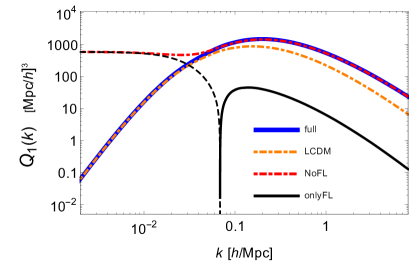
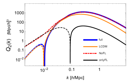
Refer to caption
Refer to caption
Figure 3: Functions Q1(k)subscript𝑄1𝑘Q_{1}(k) and Q2(k)subscript𝑄2𝑘Q_{2}(k) for F4 model: the dot-dashed red curves do not contain frame-lagging terms, the black curves have pure frame-lagging contributions (with the dashing showing the negative), and the solid blue is the full curve (with dashing for the negative in Q2subscript𝑄2Q_{2}), the dotted orange is the ΛΛ\LambdaCDM.

In Fig. 3 we show plots for the Q1subscript𝑄1Q_{1} and Q2subscript𝑄2Q_{2} functions considering their different contributions. Terms containing only frame-lagging are shown with black curves, while the red dot-dashed have no frame-lagging contributions, the sum of both gives the full Q1subscript𝑄1Q_{1} or Q2subscript𝑄2Q_{2} functions (blue curves), and the orange curves are for the ΛΛ\LambdaCDM model. For Q1subscript𝑄1Q_{1}, the cancellation due to the frame-lagging is about one part in a ten thousand at k=0.001𝑘0.001k=0.001, showing the importance of these terms at large scales. For Q2subscript𝑄2Q_{2} the cancellation is about one order of magnitude at the same scale. Analogously, in Fig. 4 we plot the R1subscript𝑅1R_{1} and R2subscript𝑅2R_{2} functions. In these cases the cancellations are not sufficient to drive these functions to their ΛΛ\LambdaCDM counterparts. More detailed inspections of their large scales behavior reveals the reason, as we show below.

To emphasize the importance of frame-lagging terms we consider first the Q1subscript𝑄1Q_{1} function. By letting the external momentum k𝑘k goes to zero in Eq. (85) we have

Q1(k0)subscript𝑄1𝑘0\displaystyle Q_{1}(k\rightarrow 0) =14π20𝑑pp2PL2(p)11𝑑x(𝒜k2x2+p22kpxk2+p22kpx)2,absent14superscript𝜋2superscriptsubscript0differential-d𝑝superscript𝑝2superscriptsubscript𝑃𝐿2𝑝superscriptsubscript11differential-d𝑥superscript𝒜superscript𝑘2superscript𝑥2superscript𝑝22𝑘𝑝𝑥superscript𝑘2superscript𝑝22𝑘𝑝𝑥2\displaystyle=\frac{1}{4\pi^{2}}\int_{0}^{\infty}dp\,p^{2}P_{L}^{2}(p)\int_{-1}^{1}dx\left(\mathcal{A}-\mathcal{B}\frac{k^{2}x^{2}+p^{2}-2kpx}{k^{2}+p^{2}-2kpx}\right)^{2}, (92)

with 𝒜=D¯a(2)(p,p)+D¯FL(2)(p,p)𝒜subscriptsuperscript¯𝐷2𝑎ppsubscriptsuperscript¯𝐷2FLpp\mathcal{A}=\bar{D}^{(2)}_{a}({\text{\bf p}},-{\text{\bf p}})+\bar{D}^{(2)}_{\text{FL}}({\text{\bf p}},-{\text{\bf p}}) and =D¯b(2)(p,p)subscriptsuperscript¯𝐷2𝑏pp\mathcal{B}=\bar{D}^{(2)}_{b}({\text{\bf p}},-{\text{\bf p}}). The D¯δI(2)subscriptsuperscript¯𝐷2𝛿𝐼\bar{D}^{(2)}_{\delta I} growth function vanishes for this configuration, otherwise it would contribute to the function 𝒜𝒜\mathcal{A}. Expanding the integrand about k=0𝑘0k=0 and discarding terms with odd powers in x𝑥x since they become zero after the angular integration, we get

(𝒜k2x2+p22kpxk2+p22kpx)2superscript𝒜superscript𝑘2superscript𝑥2superscript𝑝22𝑘𝑝𝑥superscript𝑘2superscript𝑝22𝑘𝑝𝑥2\displaystyle\left(\mathcal{A}-\mathcal{B}\frac{k^{2}x^{2}+p^{2}-2kpx}{k^{2}+p^{2}-2kpx}\right)^{2} =(𝒜)2+2(𝒜)(1x2)k2p2absentsuperscript𝒜22𝒜1superscript𝑥2superscript𝑘2superscript𝑝2\displaystyle=(\mathcal{A}-\mathcal{B})^{2}+2\mathcal{B}(\mathcal{A}-\mathcal{B})(1-x^{2})\frac{k^{2}}{p^{2}}
+(2(1x2)2+2(𝒜)(15x24x4))k4p4+𝒪(k6p6).superscript2superscript1superscript𝑥222𝒜15superscript𝑥24superscript𝑥4superscript𝑘4superscript𝑝4𝒪superscript𝑘6superscript𝑝6\displaystyle+\big{(}\mathcal{B}^{2}(1-x^{2})^{2}+2\mathcal{B}(\mathcal{A}-\mathcal{B})(-1-5x^{2}-4x^{4})\big{)}\frac{k^{4}}{p^{4}}+\mathcal{O}\left(\frac{k^{6}}{p^{6}}\right). (93)

These squeezed configurations survey large scales and then should reduce to GR. We explicitly showed in Sect. IV that 𝒜=D¯a(2)(p,p)D¯b(2)(p,p)+D¯FL(2)(p,p)=0𝒜subscriptsuperscript¯𝐷2𝑎ppsubscriptsuperscript¯𝐷2𝑏ppsubscriptsuperscript¯𝐷2FLpp0\mathcal{A}-\mathcal{B}=\bar{D}^{(2)}_{a}({\text{\bf p}},-{\text{\bf p}})-\bar{D}^{(2)}_{b}({\text{\bf p}},-{\text{\bf p}})+\bar{D}^{(2)}_{\text{FL}}({\text{\bf p}},-{\text{\bf p}})=0, thanks to the frame-lagging. By this reason the leading term that survives in Eq. (VI) is of order 𝒪((k/p)4)𝒪superscript𝑘𝑝4\mathcal{O}((k/p)^{4}), yielding

Q1(k0)subscript𝑄1𝑘0\displaystyle Q_{1}(k\rightarrow 0) =4k415π20𝑑pPL2(p)p2(D¯b(2)(p,p))2=CQ14k415π20𝑑pPL2(p)p2.absent4superscript𝑘415superscript𝜋2superscriptsubscript0differential-d𝑝superscriptsubscript𝑃𝐿2𝑝superscript𝑝2superscriptsubscriptsuperscript¯𝐷2𝑏pp2subscript𝐶subscript𝑄14superscript𝑘415superscript𝜋2superscriptsubscript0differential-d𝑝superscriptsubscript𝑃𝐿2𝑝superscript𝑝2\displaystyle=\frac{4k^{4}}{15\pi^{2}}\int_{0}^{\infty}dp\frac{P_{L}^{2}(p)}{p^{2}}(\bar{D}^{(2)}_{b}({\text{\bf p}},-{\text{\bf p}}))^{2}=C_{Q_{1}}\frac{4k^{4}}{15\pi^{2}}\int_{0}^{\infty}dp\frac{P_{L}^{2}(p)}{p^{2}}. (94)

In panel (D) of Fig. 2 we plotted D¯b(2)(p,p)subscriptsuperscript¯𝐷2𝑏pp\bar{D}^{(2)}_{b}({\text{\bf p}},-{\text{\bf p}}). It starts to depart from GR value early, at yet linear scales, but the integrand above is quickly damped by the p2superscript𝑝2p^{-2} factor, thus the net effect is small. For F4 we find CQ11.03similar-to-or-equalssubscript𝐶subscript𝑄11.03C_{Q_{1}}\simeq 1.03, for ΛΛ\LambdaCDM CQ1=I22(t=t0)1.02subscript𝐶subscript𝑄1subscriptsuperscript𝐼22𝑡subscript𝑡0similar-to-or-equals1.02C_{Q_{1}}=I^{2}_{2}(t=t_{0})\simeq 1.02, and for EdS CQ1subscript𝐶subscript𝑄1C_{Q_{1}} is exactly one. We note that there is a residual k𝑘k dependence in CQ2subscript𝐶subscript𝑄2C_{Q_{2}} since the external momentum takes small, but non-zero values. On the other hand, if we neglect the frame-lagging, then 𝒜0𝒜0\mathcal{A}-\mathcal{B}\neq 0 and the leading term in the expansion of Eq. (VI) is of order zero and we get

Q1NoFL(k0)=14π20𝑑pp2PL2(p)(D¯a(2)(p,p)D¯b(2)(p,p))2superscriptsubscript𝑄1NoFL𝑘014superscript𝜋2superscriptsubscript0differential-d𝑝superscript𝑝2superscriptsubscript𝑃𝐿2𝑝superscriptsubscriptsuperscript¯𝐷2𝑎ppsubscriptsuperscript¯𝐷2𝑏pp2Q_{1}^{\text{NoFL}}(k\rightarrow 0)=\frac{1}{4\pi^{2}}\int_{0}^{\infty}dp\,p^{2}P_{L}^{2}(p)\big{(}\bar{D}^{(2)}_{a}(-{\text{\bf p}},{\text{\bf p}})-\bar{D}^{(2)}_{b}(-{\text{\bf p}},{\text{\bf p}})\big{)}^{2} (95)

This explains that in Fig. 3 the function Q1subscript𝑄1Q_{1} without frame-lagging approaches a constant for low-k𝑘k, and due to the p2superscript𝑝2p^{2} term the function takes large values.
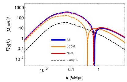
Refer to caption
Refer to caption
Figure 4: Left panel: R1(k)subscript𝑅1𝑘R_{1}(k) function: the solid red curve does not contain frame-lagging terms (with the dashing showing its negative); the dot-dashed black curve has pure frame-lagging contributions; the solid blue is the full curve; and the dotted orange is the ΛΛ\LambdaCDM. Right panel: R2(k)subscript𝑅2𝑘R_{2}(k) function: the solid red curve does not contain frame-lagging terms (with the dashing showing its negative); dashed black is the negative of pure frame-lagging contributions; solid blue is the full R2subscript𝑅2R_{2} curve (with the dashing showing its negative); and solid orange is for ΛΛ\LambdaCDM.

Analogous calculations for Q2subscript𝑄2Q_{2} leads to

Q2(k0)subscript𝑄2𝑘0\displaystyle Q_{2}(k\rightarrow 0) =k415π20𝑑pPL2(p)p2D¯b(2)(p,p)=CQ2k415π20𝑑pPL2(p)p2,absentsuperscript𝑘415superscript𝜋2superscriptsubscript0differential-d𝑝superscriptsubscript𝑃𝐿2𝑝superscript𝑝2subscriptsuperscript¯𝐷2𝑏ppsubscript𝐶subscript𝑄2superscript𝑘415superscript𝜋2superscriptsubscript0differential-d𝑝superscriptsubscript𝑃𝐿2𝑝superscript𝑝2\displaystyle=-\frac{k^{4}}{15\pi^{2}}\int_{0}^{\infty}dp\frac{P_{L}^{2}(p)}{p^{2}}\bar{D}^{(2)}_{b}(-{\text{\bf p}},{\text{\bf p}})=-C_{Q_{2}}\frac{k^{4}}{15\pi^{2}}\int_{0}^{\infty}dp\frac{P_{L}^{2}(p)}{p^{2}}, (96)

while without the frame-lagging one would obtain Q2FL(k0)k2𝑑pPL2(p)proportional-tosuperscriptsubscript𝑄2FL𝑘0superscript𝑘2differential-d𝑝subscriptsuperscript𝑃2𝐿𝑝Q_{2}^{\text{FL}}(k\rightarrow 0)\propto k^{2}\int dpP^{2}_{L}(p). The other loop functions yield

R1(k0)subscript𝑅1𝑘0\displaystyle R_{1}(k\rightarrow 0) =CR14k415π2PL(k)0𝑑pPL(p),absentsubscript𝐶subscript𝑅14superscript𝑘415superscript𝜋2subscript𝑃𝐿𝑘superscriptsubscript0differential-d𝑝subscript𝑃𝐿𝑝\displaystyle=C_{R_{1}}\frac{4k^{4}}{15\pi^{2}}P_{L}(k)\int_{0}^{\infty}dpP_{L}(p), (97)
R2(k0)subscript𝑅2𝑘0\displaystyle R_{2}(k\rightarrow 0) =CR2k415π2PL(k)0𝑑pPL(p).absentsubscript𝐶subscript𝑅2superscript𝑘415superscript𝜋2subscript𝑃𝐿𝑘superscriptsubscript0differential-d𝑝subscript𝑃𝐿𝑝\displaystyle=-C_{R_{2}}\frac{k^{4}}{15\pi^{2}}P_{L}(k)\int_{0}^{\infty}dpP_{L}(p). (98)

The difference in the derivation of R2subscript𝑅2R_{2} is that the second order growth functions are evaluated as D¯(2)(0,p)superscript¯𝐷20p\bar{D}^{(2)}(0,-{\text{\bf p}}), for which frame-lagging terms give small negative contributions, as observed in Fig. 4. The case of R1subscript𝑅1R_{1} was guessed and then tested numerically. We have checked the goodness of these approximations numerically, showing that all the CXsubscript𝐶𝑋C_{X} functions are close to unity, but more relevant for this discussion is that they depend very weakly on k𝑘k. Therefore, the Q𝑄Q and R𝑅R functions have the same k𝑘k-dependence at large scales in MG and GR.

From Eqs. (94) and (96), we now notice that the large scales modes of Q1subscript𝑄1Q_{1} and Q2subscript𝑄2Q_{2} functions receive negligible contributions from small scales, making them indistinguishable for MG models that reduce to ΛΛ\LambdaCDM at those scales, as depicted in Fig. 3. On the other hand, the R1subscript𝑅1R_{1} and R2subscript𝑅2R_{2} functions at low-k𝑘k (see Eqs. (97) and (98)) reduce to the linear power spectrum times the variance of the Lagrangian displacements, and as a result they take larger values than to those of ΛΛ\LambdaCDM, as shown in Fig. 4.

The analysis of the Q3subscript𝑄3Q_{3} function is simpler because it derives from products of linear displacement fields, thus it has the same form in MG and GR. This function is not necessary for LPT matter statistics, but it is required for computing the SPT power spectrum, as explained in Appendix A. Its large scale limit is

Q3(k0)=k410π20𝑑pPL2(p)p2.subscript𝑄3𝑘0superscript𝑘410superscript𝜋2superscriptsubscript0differential-d𝑝superscriptsubscript𝑃𝐿2𝑝superscript𝑝2Q_{3}(k\rightarrow 0)=\frac{k^{4}}{10\pi^{2}}\int_{0}^{\infty}dp\frac{P_{L}^{2}(p)}{p^{2}}. (99)

Now, for scale invariant universes with PL(p)pnproportional-tosubscript𝑃𝐿𝑝superscript𝑝𝑛P_{L}(p)\propto p^{n} as we consider in the following, we fix the external k𝑘k momentum and let the internal momentum p𝑝p goes to infinity. The equations derived above in the limit k0𝑘0k\rightarrow 0 can do this job for power law power spectra, and in this way we observe the Q𝑄Q functions have UV divergences for n1/2𝑛12n\geq 1/2 and the R𝑅R functions for n1𝑛1n\geq-1; these are the same UV divergences that have the P22subscript𝑃22P_{22} and P13subscript𝑃13P_{13} pieces of the SPT power spectrum, respectively. We notice that if frame-lagging is not considered, UV divergences for Q1subscript𝑄1Q_{1} are present for n3/2𝑛32n\geq-3/2, while for Q1subscript𝑄1Q_{1} when n>1/2𝑛12n>-1/2.


On the other hand, IR divergences may show up both at p0p0{\text{\bf p}}\rightarrow 0 and pkpk{\text{\bf p}}\rightarrow{\text{\bf k}}. In Ref. Carrasco:2013sva P22subscript𝑃22P_{22} is written in such a way both divergences appear at momentum zero. We follow that work and define

q3(k,p)=(kp)2p4(k(kp))2|kp|4PL(p)PL(|kp|).subscript𝑞3kpsuperscriptkp2superscript𝑝4superscriptkkp2superscriptkp4subscript𝑃𝐿𝑝subscript𝑃𝐿kpq_{3}({\text{\bf k}},{\text{\bf p}})=\frac{({\text{\bf k}}\cdot{\text{\bf p}})^{2}}{p^{4}}\frac{({\text{\bf k}}\cdot({\text{\bf k}}-{\text{\bf p}}))^{2}}{|{\text{\bf k}}-{\text{\bf p}}|^{4}}P_{L}(p)P_{L}(|{\text{\bf k}}-{\text{\bf p}}|). (100)

From Eqs. (114) and (120), Q3subscript𝑄3Q_{3} can be written as

Q3(k)subscript𝑄3𝑘\displaystyle Q_{3}(k) =d3p(2π)3q3(k,p)=p<|kp|d3p(2π)3q3(k,p)+p>|kp|d3p(2π)3q3(k,p)absentsuperscript𝑑3𝑝superscript2𝜋3subscript𝑞3kp𝑝kpsuperscript𝑑3𝑝superscript2𝜋3subscript𝑞3kp𝑝kpsuperscript𝑑3𝑝superscript2𝜋3subscript𝑞3kp\displaystyle=\int\frac{d^{3}p}{(2\pi)^{3}}q_{3}({\text{\bf k}},{\text{\bf p}})=\underset{p<|{\text{\bf k}}-{\text{\bf p}}|}{\int}\frac{d^{3}p}{(2\pi)^{3}}q_{3}({\text{\bf k}},{\text{\bf p}})+\underset{p>|{\text{\bf k}}-{\text{\bf p}}|}{\int}\frac{d^{3}p}{(2\pi)^{3}}q_{3}({\text{\bf k}},{\text{\bf p}})
=p<|kp|d3p(2π)3q3(k,p)+p~<|k𝐩~|d3p~(2π)3q3(k,k𝐩~)absent𝑝kpsuperscript𝑑3𝑝superscript2𝜋3subscript𝑞3kp~𝑝k~𝐩superscript𝑑3~𝑝superscript2𝜋3subscript𝑞3kk~𝐩\displaystyle=\underset{p<|{\text{\bf k}}-{\text{\bf p}}|}{\int}\frac{d^{3}p}{(2\pi)^{3}}q_{3}({\text{\bf k}},{\text{\bf p}})+\underset{\tilde{p}<|{\text{\bf k}}-\mathbf{\tilde{p}}|}{\int}\frac{d^{3}\tilde{p}}{(2\pi)^{3}}q_{3}({\text{\bf k}},{\text{\bf k}}-\mathbf{\tilde{p}})
=2p<|kp|d3p(2π)3q3(k,p).absent2𝑝kpsuperscript𝑑3𝑝superscript2𝜋3subscript𝑞3kp\displaystyle=2\!\!\!\underset{p<|{\text{\bf k}}-{\text{\bf p}}|}{\int}\frac{d^{3}p}{(2\pi)^{3}}q_{3}({\text{\bf k}},{\text{\bf p}}). (101)

In the second equality we have split the region of integration in two pieces separated by the pksimilar-to𝑝𝑘p\sim k divergence. In the second integral of the third equality we redefined the variable p=k𝐩~pk~𝐩{\text{\bf p}}={\text{\bf k}}-\mathbf{\tilde{p}}. In the last we use the symmetry q3(k,p)=q3(k,kp)subscript𝑞3kpsubscript𝑞3kkpq_{3}({\text{\bf k}},{\text{\bf p}})=q_{3}({\text{\bf k}},{\text{\bf k}}-{\text{\bf p}}). In this way, Q3(k)subscript𝑄3𝑘Q_{3}(k) has IR divergences only for p0p0{\text{\bf p}}\rightarrow 0. Fixing the external momentum, a standard computation leads to write, with a little abuse of notation,

Q3IR=k23π2PL(k)0k𝑑pPL(p)(1+p2k2+𝒪(p4k4)),superscriptsubscript𝑄3IRsuperscript𝑘23superscript𝜋2subscript𝑃𝐿𝑘superscriptsubscript0𝑘differential-d𝑝subscript𝑃𝐿𝑝1superscript𝑝2superscript𝑘2𝒪superscript𝑝4superscript𝑘4Q_{3}^{\text{IR}}=\frac{k^{2}}{3\pi^{2}}P_{L}(k)\int_{0}^{k}dpP_{L}(p)\left(1+\frac{p^{2}}{k^{2}}+\mathcal{O}\left(\frac{p^{4}}{k^{4}}\right)\right), (102)

and the leading IR divergence appears for spectral index n1𝑛1n\leq-1, while sub-leadings divergences reveal for n3𝑛3n\leq-3.

For Q2(k)subscript𝑄2𝑘Q_{2}(k), we find an IR divergence that does not appear in ΛΛ\LambdaCDM. Expanding the angular integrand of Eq. (86) about r=0𝑟0r=0 (or equivalently p=0𝑝0p=0) with power law potential and discarding odd powers of x𝑥x, we get

(1+r22rx)n/2rx(1rx)1+r22rx(𝒜(xr)21+r22rx)=(𝒜)(1n)x2p2k2+𝒪(p4k4)superscript1superscript𝑟22𝑟𝑥𝑛2𝑟𝑥1𝑟𝑥1superscript𝑟22𝑟𝑥𝒜superscript𝑥𝑟21superscript𝑟22𝑟𝑥𝒜1𝑛superscript𝑥2superscript𝑝2superscript𝑘2𝒪superscript𝑝4superscript𝑘4(1+r^{2}-2rx)^{n/2}\frac{rx(1-rx)}{1+r^{2}-2rx}\left(\mathcal{A}-\mathcal{B}\frac{(x-r)^{2}}{1+r^{2}-2rx}\right)=(\mathcal{A}-\mathcal{B})(1-n)x^{2}\frac{p^{2}}{k^{2}}+\mathcal{O}\left(\frac{p^{4}}{k^{4}}\right) (103)

Here 𝒜=D¯a(2)(0,k)D¯δI(2)(0,k)𝒜subscriptsuperscript¯𝐷2𝑎0ksubscriptsuperscript¯𝐷2𝛿𝐼0k\mathcal{A}=\bar{D}^{(2)}_{a}(0,{\text{\bf k}})-\bar{D}^{(2)}_{\delta I}(0,{\text{\bf k}}) and =D¯a(2)(0,k)subscriptsuperscript¯𝐷2𝑎0k\mathcal{B}=\bar{D}^{(2)}_{a}(0,{\text{\bf k}}), while D¯FL(2)(0,k)=0subscriptsuperscript¯𝐷2FL0k0\bar{D}^{(2)}_{\text{FL}}(0,{\text{\bf k}})=0 for this configuration. This is not the same squeezed configuration found above in Eq. (VI), and then 𝒜0𝒜0\mathcal{A}-\mathcal{B}\neq 0. As a result we get

Q2IR=16π2PL(k)0𝑑pp2PL(p)(𝒜)(1n).superscriptsubscript𝑄2IR16superscript𝜋2subscript𝑃𝐿𝑘superscriptsubscript0differential-d𝑝superscript𝑝2subscript𝑃𝐿𝑝𝒜1𝑛Q_{2}^{\text{IR}}=\frac{1}{6\pi^{2}}P_{L}(k)\int_{0}^{\infty}dp\,p^{2}P_{L}(p)(\mathcal{A}-\mathcal{B})(1-n). (104)

Although this IR divergence does not appear in ΛΛ\LambdaCDM, it is safe since is revealed for n3𝑛3n\leq-3. For R2subscript𝑅2R_{2} and Q1subscript𝑄1Q_{1} functions the IR divergences when the internal momentum is sent to zero appear for n<3𝑛3n<-3, as in ΛΛ\LambdaCDM.

On the other hand for pkpk{\text{\bf p}}\rightarrow{\text{\bf k}}, functions Q1subscript𝑄1Q_{1} and Q2subscript𝑄2Q_{2} present divergences that goes as (pk)n+2superscript𝑝𝑘𝑛2(p-k)^{n+2} and (pk)n+1superscript𝑝𝑘𝑛1(p-k)^{n+1}, respectively, which are of the same form as in ΛΛ\LambdaCDM. These results rely in the approximation of letting fixed the growth functions as D¯(2)(k,0)superscript¯𝐷2k0\bar{D}^{(2)}({\text{\bf k}},0) as follows from Eq. (90).

For R2subscript𝑅2R_{2} as pkpk{\text{\bf p}}\rightarrow{\text{\bf k}} we have the evaluation D¯(2)(k,k)superscript¯𝐷2kk\bar{D}^{(2)}(-{\text{\bf k}},{\text{\bf k}}), which is the same squeezed configuration found in Eq. (VI) for which 𝒜=0𝒜0\mathcal{A}-\mathcal{B}=0. Thus, we can substitute 𝒜𝒜\mathcal{A} for \mathcal{B} in the integrand of Eq. (89). Since this is a function of k𝑘k only it can be factorized and pulled out of the integral. Thus R2subscript𝑅2R_{2} has no IR divergence for pkpk{\text{\bf p}}\rightarrow{\text{\bf k}} as in ΛΛ\LambdaCDM. In the absence of frame-lagging 𝒜𝒜\mathcal{A}\neq\mathcal{B} and we obtain a log|pk|𝑝𝑘\log|p-k| divergence after expanding Eq. (89) about p=k𝑝𝑘p=k and performing the angular integration.


The intuition developed in this section suggest that IR and UV divergences for Q𝑄Q and R𝑅R functions are the same in MG and in ΛΛ\LambdaCDM. Though, a rigorous proof is still lacking; in particular we did not analyze the divergences of R1subscript𝑅1R_{1} function. We stress that in our derivations the role played by the frame-lagging terms is determinant, and further, we assumed MG models that converge to GR at large scales.


We finalize this section by showing the power spectrum a(k)PΨΨ𝑎𝑘subscript𝑃ΨΨa(k)\equiv P_{\nabla\cdot\Psi\,\nabla\cdot\Psi} of the divergence of Lagrangian displacement fields, iΨisubscript𝑖superscriptΨ𝑖\nabla_{i}\Psi^{i}, at 1-loop. This is given by a(k)=k1ik2jΨi(1)(k1)Ψj(1)(k2)c+k1ik2jΨi(2)(k1)Ψj(2)(k2)c+2k1ik2jΨi(1)(k1)Ψj(3)(k2)c𝑎𝑘subscriptsuperscript𝑘𝑖1subscriptsuperscript𝑘𝑗2superscriptsubscriptdelimited-⟨⟩superscriptsubscriptΨ𝑖1subscript𝑘1superscriptsubscriptΨ𝑗1subscript𝑘2𝑐subscriptsuperscript𝑘𝑖1subscriptsuperscript𝑘𝑗2superscriptsubscriptdelimited-⟨⟩superscriptsubscriptΨ𝑖2subscript𝑘1superscriptsubscriptΨ𝑗2subscript𝑘2𝑐2subscriptsuperscript𝑘𝑖1subscriptsuperscript𝑘𝑗2superscriptsubscriptdelimited-⟨⟩superscriptsubscriptΨ𝑖1subscript𝑘1superscriptsubscriptΨ𝑗3subscript𝑘2𝑐a(k)=k^{i}_{1}k^{j}_{2}\langle\Psi_{i}^{(1)}(k_{1})\Psi_{j}^{(1)}(k_{2})\rangle_{c}^{\prime}+k^{i}_{1}k^{j}_{2}\langle\Psi_{i}^{(2)}(k_{1})\Psi_{j}^{(2)}(k_{2})\rangle_{c}^{\prime}+2k^{i}_{1}k^{j}_{2}\langle\Psi_{i}^{(1)}(k_{1})\Psi_{j}^{(3)}(k_{2})\rangle_{c}^{\prime}, where the notation ()superscriptdelimited-⟨⟩\langle(\cdots)\rangle^{\prime} means that we omit a Dirac delta function. Using Eqs. (118) and (121) this is

a(k)=PL(k)+998Q1(k)+1021Q2(k),𝑎𝑘subscript𝑃𝐿𝑘998subscript𝑄1𝑘1021subscript𝑄2𝑘a(k)=P_{L}(k)+\frac{9}{98}Q_{1}(k)+\frac{10}{21}Q_{2}(k), (105)

where PL(k)subscript𝑃𝐿𝑘P_{L}(k) coincides with the linear power spectrum of matter fluctuations. In Fig. 5 we show a plot of a(k)𝑎𝑘a(k) with their different contributions. We note that the piece without frame-lagging has negative values.
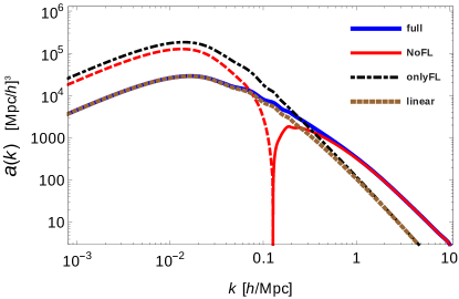
Refer to caption
Figure 5: Power spectrum a(k)𝑎𝑘a(k) of divergences of Lagrangian displacements for the F4 model: The solid blue curve is the full power spectrum, the dot-dashed black contains only frame-lagging contributions; the red curve does not contain any frame-lagging, with the dashed showing its negative; the dotted brown is for the linear theory, that coincide with the linear matter power spectrum.

VII CDM 2-point statistics

In this section we compute the power spectrum and correlation function for F4, F5 and F6 models using the schemes described in Appendix A. The building blocks are the Qisubscript𝑄𝑖Q_{i} and Risubscript𝑅𝑖R_{i} functions already computed in the previous section. As discussed in the introduction, LPT statistics are better for modeling the BAO feature while SPT is better in the broadband power spectrum, and for that reason we explore both approaches here. Specifically, we use the Convolution Lagrangian Perturbation Theory (CLPT) of Ref. Carlson:2012bu , the Lagrangian Resummation Theory (LRT) Mat08a , and the SPT* explained in Appendix A.

For our numerical computations we fix cosmological parameters to Ωm=0.281subscriptΩ𝑚0.281\Omega_{m}=0.281, Ωb=0.046subscriptΩ𝑏0.046\Omega_{b}=0.046, h=0.6970.697h=0.697, ns=0.971subscript𝑛𝑠0.971n_{s}=0.971, and σ8=0.82subscript𝜎80.82\sigma_{8}=0.82, corresponding to the best fit of the WMAP Nine-year results 2013ApJS..208…19H . The linear ΛΛ\LambdaCDM matter power spectrum is computed with the CAMB code Lewis:1999bs , and the linear MG is obtained by multiplying it by the square of linear growth factor,

PLMG(k)=D+2(k)PLΛCDM(k).superscriptsubscript𝑃𝐿MG𝑘superscriptsubscript𝐷2𝑘superscriptsubscript𝑃𝐿ΛCDM𝑘P_{L}^{\text{MG}}(k)=D_{+}^{2}(k)P_{L}^{\text{$\Lambda$CDM}}(k). (106)

We compute the CLPT power spectrum in Eq. (129) from the Hankel transformations of Eqs. (131), (132) and (133) and using FFTLog numerical methods, as described in Hamilton:1999uv .555In practice, the sums in Eqs. (137) are performed up to some maxsubscript𝑚𝑎𝑥\ell_{max}. In the code we use for this work, this maximum is adaptive in the interval k=0.001𝑘0.001k=0.0013h/Mpc3Mpc3\,h/\text{Mpc} ranging from max=10subscriptmax10\ell_{\text{max}}=10 to 30. We specifically make use of the public code released in Vlah:2016bcl .666https://github.com/martinjameswhite/CLEFT_GSM., that is supplied with precomputed ΞsubscriptΞ\Xi_{\ell} functions, defined in Vlah:2015sea , which are combinations of the X𝑋X, Y𝑌Y, V𝑉V and T𝑇T functions defined in Eqs. (125)-(128).

The LRT power spectrum, written in this section as PLRT(k)=ek2σL2PL(k)+NLsubscript𝑃LRT𝑘superscript𝑒superscript𝑘2subscriptsuperscript𝜎2𝐿subscript𝑃𝐿𝑘NLP_{\text{LRT}}(k)=e^{-k^{2}\sigma^{2}_{L}}P_{L}(k)+\text{NL}, with NL denoting the loop integrals, and

σL2=16π20𝑑pPL(p)subscriptsuperscript𝜎2𝐿16superscript𝜋2superscriptsubscript0differential-d𝑝subscript𝑃𝐿𝑝\sigma^{2}_{L}=\frac{1}{6\pi^{2}}\int_{0}^{\infty}dpP_{L}(p) (107)

the total variance of the divergence of linear Lagrangian displacements, is obtained directly by providing Eq. (142) with the Q𝑄Q and R𝑅R functions.

Since LRT and CLPT power spectra decay quickly (in k𝑘k), we expand them to obtain the 1-loop SPT* power spectrum —which in EdS coincides with the 1-loop SPT power spectrum— as explained in the Appendix A. Thus, we analyze also the power spectrum PSPT(k)=(1σL2k2)PL(k)+NLsubscript𝑃superscriptSPT𝑘1subscriptsuperscript𝜎2𝐿superscript𝑘2subscript𝑃𝐿𝑘NLP_{\text{SPT}^{*}}(k)=(1-\sigma^{2}_{L}k^{2})P_{L}(k)+\text{NL} of Eq. (139).

Refer to caption
Refer to caption
Figure 6: Ratios of power spectra to the linear corresponding models (F4 and F5) power spectrum with BAO removed at redshift z=0𝑧0z=0. Long dashed black curves are for the linear theory; dashed blue are for CLPT; solid red are for SPT*; dot-dashed brown are for LRT; and dotted green are the linear ΛΛ\LambdaCDM. The vertical line shows the scale kNL=σL1/2subscript𝑘NLsubscriptsuperscript𝜎1𝐿2k_{\text{NL}}=\sigma^{-1}_{L}/2.
Refer to caption
Refer to caption
Figure 7: Ratios of power spectra to the linear corresponding models (F6 and ΛΛ\LambdaCDM) power spectrum with BAO removed at redshift z=0𝑧0z=0. Long dashed black curves are for the linear theory; dashed blue are for CLPT; solid red are for SPT*; dot-dashed brown are for LRT. The F6 panel shows also the linear ΛΛ\LambdaCDM case, denoted with dotted green curve. The vertical line shows the scale kNL=σL1/2subscript𝑘NLsubscriptsuperscript𝜎1𝐿2k_{\text{NL}}=\sigma^{-1}_{L}/2.

In Figs. 6 and 7 we show the ratio of the different power spectra and the linear power spectrum of the considered model with the BAO removed, this is done for CLPT, LRT and SPT*, and for F4, F5, F6 and ΛΛ\LambdaCDM models at redshift z=0𝑧0z=0. Dashed blue curves correspond to the CLPT scheme, solid red are for the SPT*, brown dashed for LRT, and long-dashed black for the linear theory. As a reference, for MG models we plot the linear ΛΛ\LambdaCDM model as well (depicted by dotted green curves). The vertical lines denote the expected maximum wavelengths kmaxsubscript𝑘𝑚𝑎𝑥k_{max} of validity of the perturbative Lagrangian formalisms. For these, we adopt the prescription in Ref. Mat08a relying on the damping scale, such that kmax=σL1/2subscript𝑘𝑚𝑎𝑥superscriptsubscript𝜎L12k_{max}=\sigma_{\text{L}}^{-1}/2; other prescriptions are possible, but do not differ substantially. We note that in MG models non-linearities starts to be more relevant at larger scales since clustering is more efficient due to the extra force.
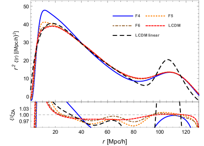
Refer to caption
Figure 8: CLPT correlation function at redshift z=0𝑧0z=0. Long dashed (black) is the linear ΛΛ\LambdaCDM model; dashed (red) is for ΛΛ\LambdaCDM in CLPT ; solid (blue) is for F4; dotted (orange) for F5; and dot-dashed (brown) is for F6. The lower panel shows the ratio with the Zel’dovich approximation in ΛΛ\LambdaCDM.

LPT formulations perform better for the correlation function; it was indeed noted that even the Zel’dovich approximation provides very good accuracy about the BAO peak; see for example Tassev:2013rta ; Whi14 for recent discussions. We compute the CLPT correlation functions given by Eq. (138). To do it we feed the code of Vlah:2015sea 777https://github.com/alejandroaviles/CLEFT. with precomputed Qisubscript𝑄𝑖Q_{i} and Risubscript𝑅𝑖R_{i} functions. We show the results in Fig. 8, with the lower panel showing the relative difference when comparing to the ΛΛ\LambdaCDM Zel’dovich approximation in the ΛΛ\LambdaCDM, which is computed from Eq. (131). At the BAO scale, the differences in the correlation among the three MG and ΛΛ\LambdaCDM models are smaller than 2%percent22\% since at these scales the fifth force is almost negligible. Soon below the BAO scales the differences depart considerably for F4, which is not surprising since this model is ruled out even at the linear level Hojjati:2015ojt .

In Figs. 9 and 10 we show the SPT* power spectra for two redshifts z=0𝑧0z=0 and z=0.5𝑧0.5z=0.5 with and without screenings. As a reference we use N𝑁N-body simulations data Liaknowled performed with the ECOSMOG code of Ref. Li:2011 . The presented data are the average of two realizations in boxes of size 1024Mpc/h1024Mpc1024\,\text{Mpc}/h and with 10243superscript102431024^{3} dark matter particles. It is difficult to tell what is the scale at which SPT* is valid since the data is noisy at large scales,888We stress that N𝑁N-body codes for MG are numerically quite expensive and are aimed mainly to test the small scales. Thus they use relatively small boxes and large scales turn out to be highly affected by cosmic variance. but we expect to have a good accuracy up to the kmaxsubscript𝑘𝑚𝑎𝑥k_{max} given above. Nevertheless, we can note that the trend line of the data is properly followed by the analytical method.
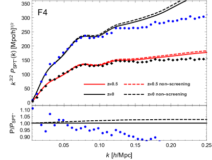
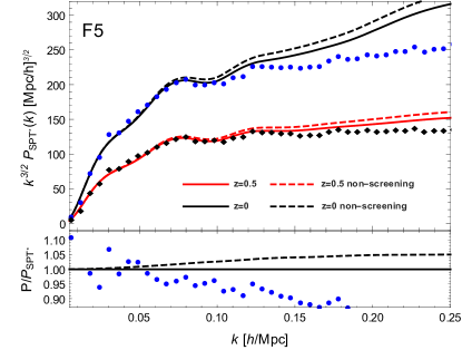
Refer to caption
Refer to caption
Figure 9: F4 and F5. SPT* power spectra with (solid curves) and without (dashed curves) screenings for models F4 and F5, at redshifts z=0𝑧0z=0 (black curves) and z=0.5𝑧0.5z=0.5 (red curves). The lower panels shows the ratio with the SPT* power spectra for z=0𝑧0z=0. The simulated data were provided by Liaknowled .
Refer to caption
Figure 10: Same as Fig. 9 but for F6.

Since small scales structures are subject to negligible tidal forces from bulk flows provided by long wavelength fluctuations, these are only affected by an overall translation which has no net effect in their matter N𝑁N-point statistics. The flaw of LRT is that bulk flows are split in q𝑞q dependent and independent pieces [see Eq. (141)] and does not cancel at zero Lagrangian separation. Indeed, in the exponential prefactor of Eq. (142) we find the term σL2subscriptsuperscript𝜎2𝐿\sigma^{2}_{L}, that has an IR divergence for power law power spectrum with spectral index n1𝑛1n\leq-1, as a consequence the bulk flows largely affect the small scales statistics, this is a manifestation of the breaking the Galilean invariance (see for example Sugiyama:2013mpa for recent discussion in LRT). This effect is observed in Fig. 6 and 7 where a deficit in the power spectrum with respect to the CLPT results is quite evident. Instead, in CLPT all linear contributions are kept in the exponential [see Eq. (129)], including the term

12XL(q)=12π2𝑑kP(k)(13j1(kq)kq)k0q260π2𝑑kk2P(k),12subscript𝑋𝐿𝑞12superscript𝜋2differential-d𝑘𝑃𝑘13subscript𝑗1𝑘𝑞𝑘𝑞𝑘0superscript𝑞260superscript𝜋2differential-d𝑘superscript𝑘2𝑃𝑘\frac{1}{2}X_{L}(q)=\frac{1}{2\pi^{2}}\int dk\,P(k)\left(\frac{1}{3}-\frac{j_{1}(kq)}{kq}\right)\,\underset{k\rightarrow 0}{\longrightarrow}\,\frac{q^{2}}{60\pi^{2}}\int dk\,k^{2}P(k), (108)

which is IR-safe for n>3𝑛3n>-3.999For power spectrum with n3𝑛3n\leq-3, tidal forces from long modes can not be neglected at any scale Carrasco:2013sva .

The SPT* power spectrum is usually written as PSPT*(k)=PL(k)+P22(k)+P13(k)subscript𝑃SPT*𝑘subscript𝑃𝐿𝑘subscript𝑃22𝑘subscript𝑃13𝑘P_{\text{SPT*}}(k)=P_{L}(k)+P_{22}(k)+P_{13}(k), in terms of Q𝑄Q and R𝑅R functions these are

P22(k)subscript𝑃22𝑘\displaystyle P_{22}(k) =998Q1(k)+37Q2(k)+12Q3(k),absent998subscript𝑄1𝑘37subscript𝑄2𝑘12subscript𝑄3𝑘\displaystyle=\frac{9}{98}Q_{1}(k)+\frac{3}{7}Q_{2}(k)+\frac{1}{2}Q_{3}(k), (109)
P11(k)subscript𝑃11𝑘\displaystyle P_{11}(k) =1021R1(k)+67R2(k)σL2k2PL(k).absent1021subscript𝑅1𝑘67subscript𝑅2𝑘superscriptsubscript𝜎𝐿2superscript𝑘2subscript𝑃𝐿𝑘\displaystyle=\frac{10}{21}R_{1}(k)+\frac{6}{7}R_{2}(k)-\sigma_{L}^{2}k^{2}P_{L}(k). (110)

The loop integrals have in general IR divergences for power law power spectrum with spectral index n<1𝑛1n<-1, but they cancel out exactly when the sum is considered. This is a consequence of the discussion above but is more general due to the equivalence principle Carrasco:2013sva ; Creminelli:2013mca . We have already found in Eq. (102) IR divergences in Q3subscript𝑄3Q_{3} when p0𝑝0p\rightarrow 0 and pksimilar-to𝑝𝑘p\sim k, which are twice that of σL2PLsubscriptsuperscript𝜎2𝐿subscript𝑃𝐿\sigma^{2}_{L}P_{L}, but in Eq. (109) Q3subscript𝑄3Q_{3} is multiplied by a 1/2121/2 factor; thus, when summing up the two SPT leading divergences cancel. This is an old known result since the work of 1983MNRAS.203..345V , and afterwards noted in 1996ApJ…456…43J ; Scoccimarro:1995if that the same should happen for sub-leading divergences; we indeed have found other sub-leading divergences for R𝑅R and Q𝑄Q functions. Our reasoning of Sect. VI suggests that the additional, sub-leading IR divergences with power spectral index n>3𝑛3n>-3 are the same as those of ΛΛ\LambdaCDM, making the theory IR-safe.

Even for MG theories with universal couplings, the principle of equivalence can be violated since some bodies may develop screening against the additional force while some others may not Hui:2009kc , but for long wavelength fluctuations this is irrelevant as long as they essentially exert only the Newtonian force upon the small structures. A brute force approach is elusive, but the absence of IR divergences (for n>3𝑛3n>-3) in MG theories that reduce to GR at large scales is in principle ensured by the equivalence principle Valageas:2013cma .

VIII Conclusions

In this work we found a generalization to alternative theories of gravity for the Lagrangian displacement field up to third order in perturbation theory. In doing this, an LPT theory for the study of large scale structure formation was developed. Our formalism is suitable for Horndeski models Bose:2016qun , this is the same range of validity that share several investigations in SPT that came after to the pioneering work of Ref. 2009PhRvD..79l3512K . The basic requirement is that the theory can be recasted as a scalar tensor gravity at linear order, all non linear contributions to the Klein-Gordon equation, including possible kinetic terms, can be written as sources and treated perturbatively. In theories that have a screening mechanism these contributions are responsible to the recover GR at small scales, by making the Laplacian of the scalar field negligible.

Since in LPT is standard to work in q𝑞q-Fourier space, one needs to transform the Poisson equation accordingly. In these theories the Poisson equation has two sources: the standard source of matter perturbations can be written in terms of Lagrangian displacement straightforwardly due to mass conservation, but the terms arising from the scalar field must be properly transformed. By doing it, terms to compensate spatial derivatives in Eulerian space appear into the theory, we call these geometrical contributions frame-lagging terms, and have a crucial role in the LPT for MG, which is more evident at large scales where the theory should reduce to GR. We have discussed this limit from different perspectives. A special one is the 1-dimensional collapse for which the Zel’dovich approximation is exact (up to shell-crossing) in ΛΛ\LambdaCDM, while in MG this is not the case since the force mediated by the scalar field does not decay as the square of the inverse of the distance. But at scales larger than the range of the fifth force the only force in play is the standard Newtonian force and we have to recover Zel’dovich as the exact solution, or in other words, the Lagrangian displacement growth functions at orders higher than 1 should vanish. The formalism presented here is capable to capture this physical fact, mathematically through cancellations provided by the frame-lagging contributions.

Throughout this article we apply the formalism by using the Hu-Sawicky f(R)𝑓𝑅f(R) theory Hu:2007nk , more precisely to the so-called F4, F5, and F6 models. We compute 2-point statistics both for the Lagrangian displacement and for the matter perturbations. For the matter power spectrum we use recent N𝑁N-body simulations Liaknowled as a reference. LPT is very successful in reproducing the acoustic peak in the correlation function, and we use two different resummation schemes: CLPT and LRT. Though, LPT is not satisfactory in following the broadband power spectrum. For this reason, we also use a scheme that reduces to SPT for the EdS case Mat08a —in MG it is not clear if one recovers SPT exactly since frame-lagging terms do not seem to cancel out— showing good agreement between the analytic theory and simulations.

We further discussed UV and IR divergences in matter and Lagrangian displacement statistics. Our analysis is not exhaustive, but it suggests that the schemes of SPT* and CLPT are IR-safe in MG.

Acknowledgements.
The authors would like to thank Baojiu Li for useful discussions and for sharing the N𝑁N-body simulation data. We also thank to Zvonimir Vlah and Matteo Cataneo for suggestions and discussions. A.A. is supported by Cátedras CONACyT project No.574. The authors acknowledge financial support from CONACyT Project 269652 and Fronteras Project 281.

Appendix A Lagrangian displacement polyspectra and the matter power spectrum

This appendix briefly reviews the methods we use to compute the power spectrum and the correlation function. For completeness we write the relevant equations but we refer the reader to the original papers for detailed derivations.

The matter power spectrum in LPT is given by TayHam96

PLPT(k)=d3qeikq(eikΔ1),subscript𝑃LPTksuperscript𝑑3𝑞superscript𝑒𝑖kqdelimited-⟨⟩superscript𝑒𝑖kΔ1P_{\text{LPT}}({\text{\bf k}})=\int d^{3}qe^{-i{\text{\bf k}}\cdot{\text{\bf q}}}\left(\langle e^{-i{\text{\bf k}}\cdot\Delta}\rangle-1\right), (111)

where Δi=Ψi(q2)Ψi(q1)subscriptΔ𝑖subscriptΨ𝑖subscriptq2subscriptΨ𝑖subscriptq1\Delta_{i}=\Psi_{i}({\text{\bf q}}_{2})-\Psi_{i}({\text{\bf q}}_{1}) are the Lagrangian displacement differences, and q=q2q1qsubscriptq2subscriptq1{\text{\bf q}}={\text{\bf q}}_{2}-{\text{\bf q}}_{1} the Lagrangian coordinate difference. By using the cumulant expansion theorem we can recast the power spectrum as Carlson:2012bu

(2π)2δD(k)+PLPT(k)=d3qeikqexp[12kikjAij(q)+i6kikjkkWijk(q)],superscript2𝜋2subscript𝛿𝐷ksubscript𝑃LPTksuperscript𝑑3𝑞superscript𝑒𝑖kq12subscript𝑘𝑖subscript𝑘𝑗subscript𝐴𝑖𝑗q𝑖6subscript𝑘𝑖subscript𝑘𝑗subscript𝑘𝑘subscript𝑊𝑖𝑗𝑘q(2\pi)^{2}\delta_{D}({\text{\bf k}})+P_{\text{LPT}}({\text{\bf k}})=\int d^{3}qe^{-i{\text{\bf k}}\cdot{\text{\bf q}}}\exp\left[-\frac{1}{2}k_{i}k_{j}A_{ij}({\text{\bf q}})+\frac{i}{6}k_{i}k_{j}k_{k}W_{ijk}({\text{\bf q}})\right], (112)

where Aij=ΔiΔjcsubscript𝐴𝑖𝑗subscriptdelimited-⟨⟩subscriptΔ𝑖subscriptΔ𝑗𝑐A_{ij}=\langle\Delta_{i}\Delta_{j}\rangle_{c} and Wijk=ΔiΔjΔkcsubscript𝑊𝑖𝑗𝑘subscriptdelimited-⟨⟩subscriptΔ𝑖subscriptΔ𝑗subscriptΔ𝑘𝑐W_{ijk}=\langle\Delta_{i}\Delta_{j}\Delta_{k}\rangle_{c}. Here we show terms up to third order in the Lagrangian displacement since we are interested in the first, 1-loop corrections to the matter two point functions. The products ΔiΔjsubscriptΔ𝑖subscriptΔ𝑗\Delta_{i}\Delta_{j} have contributions evaluated at the same point, the so-called zero-lag, and contributions given at a separation q.

The direct computation of the LPT power spectrum of Eq. (112) is difficult since it involves highly oscillatory integrands. This has been done in Vlah:2014nta by using expansions in spherical Bessel functions (see below) and in Sugiyama:2013mpa by similar methods involving Legendre expansions of the Lagrangian displacement differences. In part because of these numerical complications, alternative resummation schemes that Taylor expand some terms in the exponential of Eq. (112) exist in the literature. We below review those we use in this work.

We first define the polyspectra Ci1iN(n1nN)(k1,,kN)subscriptsuperscript𝐶subscript𝑛1subscript𝑛𝑁subscript𝑖1subscript𝑖𝑁subscriptk1subscriptk𝑁C^{(n_{1}\cdots n_{N})}_{i_{1}\cdots i_{N}}({\text{\bf k}}_{1},\dots,{\text{\bf k}}_{N}) at order (n1++nN)subscript𝑛1subscript𝑛𝑁(n_{1}+\cdots+n_{N}) as in Mat08a

Ψ(n1)i1(k1)Ψ(nN)iN(kN)c=(i)N2(2π)3δD(k1++kN)Ci1iN(n1nN)(k1,,kN),subscriptdelimited-⟨⟩superscriptΨsubscript𝑛1subscript𝑖1subscriptk1superscriptΨsubscript𝑛𝑁subscript𝑖𝑁subscriptk𝑁𝑐superscript𝑖𝑁2superscript2𝜋3subscript𝛿𝐷subscriptk1subscriptk𝑁subscriptsuperscript𝐶subscript𝑛1subscript𝑛𝑁subscript𝑖1subscript𝑖𝑁subscriptk1subscriptk𝑁\langle\Psi^{(n_{1})i_{1}}({\text{\bf k}}_{1})\cdots\Psi^{(n_{N})i_{N}}({\text{\bf k}}_{N})\rangle_{c}=(-i)^{N-2}(2\pi)^{3}\delta_{D}({\text{\bf k}}_{1}+\cdots+{\text{\bf k}}_{N})C^{(n_{1}\cdots n_{N})}_{i_{1}\cdots i_{N}}({\text{\bf k}}_{1},\dots,{\text{\bf k}}_{N}), (113)

which in terms of the Lagrangian displacement kernels can be written as

Cij(11)(k)subscriptsuperscript𝐶11𝑖𝑗k\displaystyle C^{(11)}_{ij}({\text{\bf k}}) =Li(1)(k)Lj(1)(k)PL(k),absentsubscriptsuperscript𝐿1𝑖ksubscriptsuperscript𝐿1𝑗ksubscript𝑃𝐿𝑘\displaystyle=L^{(1)}_{i}({\text{\bf k}})L^{(1)}_{j}({\text{\bf k}})P_{L}(k), (114)
Cij(22)(k)subscriptsuperscript𝐶22𝑖𝑗k\displaystyle C^{(22)}_{ij}({\text{\bf k}}) =12d3p(2π)3Li(2)(p,kp)Lj(2)(p,kp)PL(p)PL(|kp|),absent12superscript𝑑3𝑝superscript2𝜋3subscriptsuperscript𝐿2𝑖pkpsubscriptsuperscript𝐿2𝑗pkpsubscript𝑃𝐿𝑝subscript𝑃𝐿kp\displaystyle=\frac{1}{2}\int\frac{d^{3}p}{(2\pi)^{3}}L^{(2)}_{i}({\text{\bf p}},{\text{\bf k}}-{\text{\bf p}})L^{(2)}_{j}({\text{\bf p}},{\text{\bf k}}-{\text{\bf p}})P_{L}(p)P_{L}(|{\text{\bf k}}-{\text{\bf p}}|), (115)
Cij(13)(k)=Cij(31)(k)subscriptsuperscript𝐶13𝑖𝑗ksubscriptsuperscript𝐶31𝑖𝑗k\displaystyle C^{(13)}_{ij}({\text{\bf k}})=C^{(31)}_{ij}({\text{\bf k}}) =12Li(1)(k)PL(k)d3p(2π)3Lj(3)symm(k,p,p)PL(p),absent12subscriptsuperscript𝐿1𝑖ksubscript𝑃𝐿𝑘superscript𝑑3𝑝superscript2𝜋3subscriptsuperscript𝐿3𝑠𝑦𝑚𝑚𝑗kppsubscript𝑃𝐿𝑝\displaystyle=\frac{1}{2}L^{(1)}_{i}({\text{\bf k}})P_{L}(k)\int\frac{d^{3}p}{(2\pi)^{3}}L^{(3)symm}_{j}({\text{\bf k}},-{\text{\bf p}},{\text{\bf p}})P_{L}(p), (116)
Cijk(112)(k1,k2,k3)=Cjki(121)(k2,k3,k1)subscriptsuperscript𝐶112𝑖𝑗𝑘subscriptk1subscriptk2subscriptk3subscriptsuperscript𝐶121𝑗𝑘𝑖subscriptk2subscriptk3subscriptk1\displaystyle C^{(112)}_{ijk}({\text{\bf k}}_{1},{\text{\bf k}}_{2},{\text{\bf k}}_{3})=C^{(121)}_{jki}({\text{\bf k}}_{2},{\text{\bf k}}_{3},{\text{\bf k}}_{1}) =Ckij(211)(k3,k1,k1)=Li(1)(k1)Lj(1)(k2)Lk(2)(k1,k2)PL(k1)PL(k2).absentsubscriptsuperscript𝐶211𝑘𝑖𝑗subscriptk3subscriptk1subscriptk1subscriptsuperscript𝐿1𝑖subscriptk1subscriptsuperscript𝐿1𝑗subscriptk2subscriptsuperscript𝐿2𝑘subscriptk1subscriptk2subscript𝑃𝐿subscript𝑘1subscript𝑃𝐿subscript𝑘2\displaystyle=C^{(211)}_{kij}({\text{\bf k}}_{3},{\text{\bf k}}_{1},{\text{\bf k}}_{1})=-L^{(1)}_{i}({\text{\bf k}}_{1})L^{(1)}_{j}({\text{\bf k}}_{2})L^{(2)}_{k}({\text{\bf k}}_{1},{\text{\bf k}}_{2})P_{L}(k_{1})P_{L}(k_{2}). (117)

Higher order polyspectra do not enter in 1-loop calculations. The following scalar functions are constructed

Q1(k)subscript𝑄1𝑘\displaystyle Q_{1}(k) =989kikjCij(22)(k),absent989subscript𝑘𝑖subscript𝑘𝑗superscriptsubscript𝐶𝑖𝑗22𝑘\displaystyle=\frac{98}{9}k_{i}k_{j}C_{ij}^{(22)}(k), (118)
Q2(k)subscript𝑄2𝑘\displaystyle Q_{2}(k) =73kikjkkd3p(2π)3Cijk(211)(k,p,pk),absent73subscript𝑘𝑖subscript𝑘𝑗subscript𝑘𝑘superscript𝑑3𝑝superscript2𝜋3superscriptsubscript𝐶𝑖𝑗𝑘211kppk\displaystyle=\frac{7}{3}k_{i}k_{j}k_{k}\int\frac{d^{3}p}{(2\pi)^{3}}C_{ijk}^{(211)}({\text{\bf k}},-{\text{\bf p}},{\text{\bf p}}-{\text{\bf k}}), (119)
Q3(k)subscript𝑄3𝑘\displaystyle Q_{3}(k) =kikjkkkld3p(2π)3Cij(11)(p)Ckl(11)(kp),absentsubscript𝑘𝑖subscript𝑘𝑗subscript𝑘𝑘subscript𝑘𝑙superscript𝑑3𝑝superscript2𝜋3subscriptsuperscript𝐶11𝑖𝑗psubscriptsuperscript𝐶11𝑘𝑙kp\displaystyle=k_{i}k_{j}k_{k}k_{l}\int\frac{d^{3}p}{(2\pi)^{3}}C^{(11)}_{ij}({\text{\bf p}})C^{(11)}_{kl}({\text{\bf k}}-{\text{\bf p}}), (120)
R1(k)subscript𝑅1𝑘\displaystyle R_{1}(k) =215kikjCij(13)(k),absent215subscript𝑘𝑖subscript𝑘𝑗superscriptsubscript𝐶𝑖𝑗13𝑘\displaystyle=\frac{21}{5}k_{i}k_{j}C_{ij}^{(13)}(k), (121)
R2(k)subscript𝑅2𝑘\displaystyle R_{2}(k) =73kikjkkd3p(2π)3Cijk(112)(k,p,pk)=73kikjkkd3p(2π)3Cijk(121)(k,p,pk).absent73subscript𝑘𝑖subscript𝑘𝑗subscript𝑘𝑘superscript𝑑3𝑝superscript2𝜋3superscriptsubscript𝐶𝑖𝑗𝑘112kppk73subscript𝑘𝑖subscript𝑘𝑗subscript𝑘𝑘superscript𝑑3𝑝superscript2𝜋3superscriptsubscript𝐶𝑖𝑗𝑘121kppk\displaystyle=\frac{7}{3}k_{i}k_{j}k_{k}\int\frac{d^{3}p}{(2\pi)^{3}}C_{ijk}^{(112)}({\text{\bf k}},-{\text{\bf p}},{\text{\bf p}}-{\text{\bf k}})=\frac{7}{3}k_{i}k_{j}k_{k}\int\frac{d^{3}p}{(2\pi)^{3}}C_{ijk}^{(121)}({\text{\bf k}},-{\text{\bf p}},{\text{\bf p}}-{\text{\bf k}}). (122)

Notice these functions are all of order 𝒪(PL2)𝒪superscriptsubscript𝑃𝐿2\mathcal{O}(P_{L}^{2}). By using decomposition in vectors q^isubscript^𝑞𝑖\hat{q}_{i} the spectra and bispectra of Lagrangian displacement differences take the form Carlson:2012bu ; Vlah:2014nta

Aij(q)subscript𝐴𝑖𝑗q\displaystyle A_{ij}({\text{\bf q}}) =X(q)δij+Y(q)q^iq^jabsent𝑋𝑞subscript𝛿𝑖𝑗𝑌𝑞subscript^𝑞𝑖subscript^𝑞𝑗\displaystyle=X(q)\delta_{ij}+Y(q)\hat{q}_{i}\hat{q}_{j} (123)
Wijk(q)subscript𝑊𝑖𝑗𝑘q\displaystyle W_{ijk}({\text{\bf q}}) =V(q)q^{iδjk}+T(q)q^iq^jq^k\displaystyle=V(q)\hat{q}_{\{i}\delta_{jk\}}+T(q)\hat{q}_{i}\hat{q}_{j}\hat{q}_{k} (124)

with

X(q)𝑋𝑞\displaystyle X(q) =1π20𝑑k(PL(k)+998Q1(k)+1021R1(k))(13j1(kq)kq)absent1superscript𝜋2subscriptsuperscript0differential-d𝑘subscript𝑃𝐿𝑘998subscript𝑄1𝑘1021subscript𝑅1𝑘13subscript𝑗1𝑘𝑞𝑘𝑞\displaystyle=\frac{1}{\pi^{2}}\int^{\infty}_{0}dk\left(P_{L}(k)+\frac{9}{98}Q_{1}(k)+\frac{10}{21}R_{1}(k)\right)\left(\frac{1}{3}-\frac{j_{1}(kq)}{kq}\right) (125)
Y(q)𝑌𝑞\displaystyle Y(q) =1π20𝑑k(PL(k)+998Q1(k)+1021R1(k))j2(kq)absent1superscript𝜋2subscriptsuperscript0differential-d𝑘subscript𝑃𝐿𝑘998subscript𝑄1𝑘1021subscript𝑅1𝑘subscript𝑗2𝑘𝑞\displaystyle=\frac{1}{\pi^{2}}\int^{\infty}_{0}dk\left(P_{L}(k)+\frac{9}{98}Q_{1}(k)+\frac{10}{21}R_{1}(k)\right)j_{2}(kq) (126)
V(q)𝑉𝑞\displaystyle V(q) =321π20dkk(Q1(k)3Q2(k)+2R1(k)6R2(k))j1(kq)15T(q),absent321superscript𝜋2superscriptsubscript0𝑑𝑘𝑘subscript𝑄1𝑘3subscript𝑄2𝑘2subscript𝑅1𝑘6subscript𝑅2𝑘subscript𝑗1subscript𝑘𝑞15𝑇𝑞\displaystyle=-\frac{3}{21\pi^{2}}\int_{0}^{\infty}\frac{dk}{k}(Q_{1}(k)-3Q_{2}(k)+2R_{1}(k)-6R_{2}(k))j_{1}(k_{q})-\frac{1}{5}T(q), (127)
T(q)𝑇𝑞\displaystyle T(q) =914π20dkk(Q1(k)+2Q2(k)+2R1(k)+4R2(k))j3(kq),absent914superscript𝜋2superscriptsubscript0𝑑𝑘𝑘subscript𝑄1𝑘2subscript𝑄2𝑘2subscript𝑅1𝑘4subscript𝑅2𝑘subscript𝑗3subscript𝑘𝑞\displaystyle=-\frac{9}{14\pi^{2}}\int_{0}^{\infty}\frac{dk}{k}(Q_{1}(k)+2Q_{2}(k)+2R_{1}(k)+4R_{2}(k))j_{3}(k_{q}), (128)

where PL(k)subscript𝑃𝐿𝑘P_{L}(k) is the linear matter power spectrum. (In general “L𝐿L” denotes a linear piece and “loop” a pure 1-loop piece.) These functions vanish as Lagrangian coordinates separation goes to zero, implying that the power spectrum does not have contribution for arbitrary small scales. This is consistent with Eq. (111).

The formalism of Convolution Lagrangian Perturbation Theory (CLPT) as presented in Vlah:2015sea relies on expanding the loop contributions of Eq. (112) while keeping the linear terms in the exponential,101010CLPT was introduced in Carlson:2012bu where also the Aijloopsuperscriptsubscript𝐴𝑖𝑗loopA_{ij}^{\text{loop}} was kept exponentiated. leading to

(2π)3δD(k)+PCLPT(k)=d3qeikqexp(12kikjAijL(q))[112kikjAijloop(q)+i6kikjkkWijkloop(q)].superscript2𝜋3subscript𝛿Dksubscript𝑃CLPT𝑘superscript𝑑3𝑞superscript𝑒𝑖kq12subscript𝑘𝑖subscript𝑘𝑗superscriptsubscript𝐴𝑖𝑗𝐿qdelimited-[]112subscript𝑘𝑖subscript𝑘𝑗superscriptsubscript𝐴𝑖𝑗loopq𝑖6superscript𝑘𝑖superscript𝑘𝑗superscript𝑘𝑘superscriptsubscript𝑊𝑖𝑗𝑘loopq(2\pi)^{3}\delta_{\text{D}}({\text{\bf k}})+P_{\text{CLPT}}(k)=\int d^{3}qe^{-i{\text{\bf k}}\cdot{\text{\bf q}}}\exp\left(-\frac{1}{2}k_{i}k_{j}A_{ij}^{L}({\text{\bf q}})\right)\left[1-\frac{1}{2}k_{i}k_{j}A_{ij}^{\text{loop}}({\text{\bf q}})+\frac{i}{6}k^{i}k^{j}k^{k}W_{ijk}^{\text{loop}}({\text{\bf q}})\right]. (129)

This can be separated in Zel’dovich and loops contributions as

PCLPT(k)=PZA(k)+PA(k)+PW(k)subscript𝑃CLPT𝑘subscript𝑃ZA𝑘subscript𝑃𝐴𝑘subscript𝑃𝑊𝑘P_{\text{CLPT}}(k)=P_{\text{ZA}}(k)+P_{A}(k)+P_{W}(k) (130)

with (for k0k0{\text{\bf k}}\neq 0)

PZA(k)subscript𝑃ZA𝑘\displaystyle P_{\text{ZA}}(k) =2π0𝑑qq2e12k2XL11𝑑μexp(iμkq12μ2k2YL)absent2𝜋superscriptsubscript0differential-d𝑞superscript𝑞2superscript𝑒12superscript𝑘2subscript𝑋𝐿subscriptsuperscript11differential-d𝜇𝑖𝜇𝑘𝑞12superscript𝜇2superscript𝑘2subscript𝑌𝐿\displaystyle=2\pi\int_{0}^{\infty}dq\,q^{2}e^{-\frac{1}{2}k^{2}X_{L}}\int^{1}_{-1}d\mu\exp\left(i\mu kq-\frac{1}{2}\mu^{2}k^{2}Y_{L}\right) (131)
PA(k)subscript𝑃𝐴𝑘\displaystyle P_{A}(k) =2π0𝑑qq2e12k2XL11𝑑μ(12k2Xloop+12k2μ2Yloop)exp(iμkq12μ2k2YL)absent2𝜋superscriptsubscript0differential-d𝑞superscript𝑞2superscript𝑒12superscript𝑘2subscript𝑋𝐿subscriptsuperscript11differential-d𝜇12superscript𝑘2subscript𝑋loop12superscript𝑘2superscript𝜇2subscript𝑌loop𝑖𝜇𝑘𝑞12superscript𝜇2superscript𝑘2subscript𝑌𝐿\displaystyle=-2\pi\int_{0}^{\infty}dq\,q^{2}e^{-\frac{1}{2}k^{2}X_{L}}\int^{1}_{-1}d\mu\left(\frac{1}{2}k^{2}X_{\text{loop}}+\frac{1}{2}k^{2}\mu^{2}Y_{\text{loop}}\right)\exp\left(i\mu kq-\frac{1}{2}\mu^{2}k^{2}Y_{L}\right) (132)
PW(k)subscript𝑃𝑊𝑘\displaystyle P_{W}(k) =2π0𝑑qq2e12k2XL11𝑑μ(i2k3μV+i2k3μ3T12k2Yloop)exp(iμkq12μ2k2YL).absent2𝜋superscriptsubscript0differential-d𝑞superscript𝑞2superscript𝑒12superscript𝑘2subscript𝑋𝐿subscriptsuperscript11differential-d𝜇𝑖2superscript𝑘3𝜇𝑉𝑖2superscript𝑘3superscript𝜇3𝑇12superscript𝑘2subscript𝑌loop𝑖𝜇𝑘𝑞12superscript𝜇2superscript𝑘2subscript𝑌𝐿\displaystyle=-2\pi\int_{0}^{\infty}dq\,q^{2}e^{-\frac{1}{2}k^{2}X_{L}}\int^{1}_{-1}d\mu\left(\frac{i}{2}k^{3}\mu V+\frac{i}{2}k^{3}\mu^{3}T\frac{1}{2}k^{2}Y_{\text{loop}}\right)\exp\left(i\mu kq-\frac{1}{2}\mu^{2}k^{2}Y_{L}\right). (133)

By using the expansions Vlah:2014nta ; Vlah:2015sea

11𝑑μeiμA+μ2Bsubscriptsuperscript11differential-d𝜇superscript𝑒𝑖𝜇𝐴superscript𝜇2𝐵\displaystyle\int^{1}_{-1}d\mu e^{i\mu A+\mu^{2}B} =2eB=0(2BA)j(A),absent2superscript𝑒𝐵superscriptsubscript0superscript2𝐵𝐴subscript𝑗𝐴\displaystyle=2e^{B}\sum_{\ell=0}^{\infty}\left(-\frac{2B}{A}\right)^{\ell}j_{\ell}(A), (134)
11𝑑μμeiμA+μ2Bsubscriptsuperscript11differential-d𝜇𝜇superscript𝑒𝑖𝜇𝐴superscript𝜇2𝐵\displaystyle\int^{1}_{-1}d\mu\mu e^{i\mu A+\mu^{2}B} =2ieB=0(2BA)j+1(A),absent2𝑖superscript𝑒𝐵superscriptsubscript0superscript2𝐵𝐴subscript𝑗1𝐴\displaystyle=2ie^{B}\sum_{\ell=0}^{\infty}\left(-\frac{2B}{A}\right)^{\ell}j_{\ell+1}(A), (135)
11𝑑μμ2eiμA+μ2Bsubscriptsuperscript11differential-d𝜇superscript𝜇2superscript𝑒𝑖𝜇𝐴superscript𝜇2𝐵\displaystyle\int^{1}_{-1}d\mu\mu^{2}e^{i\mu A+\mu^{2}B} =2eB=0(1+lB)(2BA)j(A),absent2superscript𝑒𝐵superscriptsubscript01𝑙𝐵superscript2𝐵𝐴subscript𝑗𝐴\displaystyle=2e^{B}\sum_{\ell=0}^{\infty}\left(1+\frac{l}{B}\right)\left(-\frac{2B}{A}\right)^{\ell}j_{\ell}(A), (136)
11𝑑μμ3eiμA+μ2Bsubscriptsuperscript11differential-d𝜇superscript𝜇3superscript𝑒𝑖𝜇𝐴superscript𝜇2𝐵\displaystyle\int^{1}_{-1}d\mu\mu^{3}e^{i\mu A+\mu^{2}B} =2ieB=0(1+lB)(2BA)j+1(A),absent2𝑖superscript𝑒𝐵superscriptsubscript01𝑙𝐵superscript2𝐵𝐴subscript𝑗1𝐴\displaystyle=2ie^{B}\sum_{\ell=0}^{\infty}\left(1+\frac{l}{B}\right)\left(-\frac{2B}{A}\right)^{\ell}j_{\ell+1}(A), (137)

the integrals in Eqs.(131), (132) and (133) reduce to one-dimensional Hankel transformations.

In the CLPT scheme, the correlation function can be written compactly by Fourier transforming the power spectrum of Eq. (129) and using Gaussian integrations, resulting in

1+ξCLPT(r)=d3q(2π)3det[AijL]2e12AijL(riqi)(rjqj)[112GijAijloop+16ΓijkWijkloop]1subscript𝜉CLPT𝑟superscript𝑑3𝑞superscript2𝜋3superscriptdelimited-[]subscriptsuperscript𝐴𝐿𝑖𝑗2superscript𝑒12subscriptsuperscript𝐴𝐿𝑖𝑗subscript𝑟𝑖subscript𝑞𝑖subscript𝑟𝑗subscript𝑞𝑗delimited-[]112subscript𝐺𝑖𝑗subscriptsuperscript𝐴loop𝑖𝑗16subscriptΓ𝑖𝑗𝑘superscriptsubscript𝑊𝑖𝑗𝑘loop1+\xi_{\text{CLPT}}(r)=\int\frac{d^{3}q}{(2\pi)^{3}\det[A^{L}_{ij}]^{2}}e^{\frac{1}{2}A^{L}_{ij}(r_{i}-q_{i})(r_{j}-q_{j})}\left[1-\frac{1}{2}G_{ij}A^{\text{loop}}_{ij}+\frac{1}{6}\Gamma_{ijk}W_{ijk}^{\text{loop}}\right] (138)

where Gij=Aij1gigjsubscript𝐺𝑖𝑗subscriptsuperscript𝐴1𝑖𝑗subscript𝑔𝑖subscript𝑔𝑗G_{ij}=A^{-1}_{ij}-g_{i}g_{j}, Γijk=Aij1gk+Ajk1gi+Aki1gjgigjgksubscriptΓ𝑖𝑗𝑘subscriptsuperscript𝐴1𝑖𝑗subscript𝑔𝑘subscriptsuperscript𝐴1𝑗𝑘subscript𝑔𝑖subscriptsuperscript𝐴1𝑘𝑖subscript𝑔𝑗subscript𝑔𝑖subscript𝑔𝑗subscript𝑔𝑘\Gamma_{ijk}=A^{-1}_{ij}g_{k}+A^{-1}_{jk}g_{i}+A^{-1}_{ki}g_{j}-g_{i}g_{j}g_{k}, and gi=Aij1(rjqj)subscript𝑔𝑖subscriptsuperscript𝐴1𝑖𝑗subscript𝑟𝑗subscript𝑞𝑗g_{i}=A^{-1}_{ij}(r_{j}-q_{j}).


Now, a straightforward expansion of the exponential in Eq. (129) leads to Vlah:2014nta ; Vlah:2015sea

PSPT*=PL(k)+1021R1(k)+67R2(k)+998Q1(k)+37Q2(k)+12Q3(k)σL2k2PL(k)subscript𝑃SPT*subscript𝑃𝐿𝑘1021subscript𝑅1𝑘67subscript𝑅2𝑘998subscript𝑄1𝑘37subscript𝑄2𝑘12subscript𝑄3𝑘subscriptsuperscript𝜎2𝐿superscript𝑘2subscript𝑃𝐿𝑘P_{\text{SPT*}}=P_{L}(k)+\frac{10}{21}R_{1}(k)+\frac{6}{7}R_{2}(k)+\frac{9}{98}Q_{1}(k)+\frac{3}{7}Q_{2}(k)+\frac{1}{2}Q_{3}(k)-\sigma^{2}_{L}k^{2}P_{L}(k) (139)

where

σL2=12XL(q)=16π20𝑑kPL(k)subscriptsuperscript𝜎2𝐿12subscript𝑋𝐿𝑞16superscript𝜋2subscriptsuperscript0differential-d𝑘subscript𝑃𝐿𝑘\sigma^{2}_{L}=\frac{1}{2}X_{L}(q\rightarrow\infty)=\frac{1}{6\pi^{2}}\int^{\infty}_{0}dkP_{L}(k) (140)

is the 1-dimensional Lagrangian displacement variance. The power spectrum of Eq. (139) coincides with the SPT power spectrum in the ΛΛ\LambdaCDM case. Note that this may not be the case for MG, since it is not clear that the frame-lagging terms cancel out, and SPT should be free of these terms. Nevertheless, the behavior the power spectrum in this scheme is similar to what is expected from an SPT theory, then we use it in Sect. VII and denote it as SPT*.

Other scheme widely used in the literature is the Lagrangian Resummation Theory (LRT) of Matsubara Mat08a , here the Aijsubscript𝐴𝑖𝑗A_{ij} matrix splits as

Aij=X(q)δij+(X(q)X(q))δij+Y(q)q^iq^jsubscript𝐴𝑖𝑗𝑋𝑞subscript𝛿𝑖𝑗𝑋𝑞𝑋𝑞subscript𝛿𝑖𝑗𝑌𝑞subscript^𝑞𝑖subscript^𝑞𝑗A_{ij}=X(q\rightarrow\infty)\delta_{ij}+(X(q)-X(q\rightarrow\infty))\delta_{ij}+Y(q)\hat{q}_{i}\hat{q}_{j} (141)

and the zero-lag term X(q)=2σ2𝑋𝑞2superscript𝜎2X(q\rightarrow\infty)=2\sigma^{2} is kept in the exponential while the rest is expanded, leading to

P1-loopLRT(k)=ek2σL2(PL(k)+998Q1(k)+1021R1(k)+37Q2(k)+67R2(k)+12Q3(k)).superscriptsubscript𝑃1-loopLRTksuperscript𝑒superscript𝑘2subscriptsuperscript𝜎2𝐿subscript𝑃𝐿𝑘998subscript𝑄1𝑘1021subscript𝑅1𝑘37subscript𝑄2𝑘67subscript𝑅2𝑘12subscript𝑄3𝑘P_{\text{1-loop}}^{\text{LRT}}({\text{\bf k}})=e^{-k^{2}\sigma^{2}_{L}}\left(P_{L}(k)+\frac{9}{98}Q_{1}(k)+\frac{10}{21}R_{1}(k)+\frac{3}{7}Q_{2}(k)+\frac{6}{7}R_{2}(k)+\frac{1}{2}Q_{3}(k)\right). (142)

(This equation coincides with Eq. (35) of Mat08a .) By a further expansion of the exponential we arrive back at Eq. (139).

The exponential prefactor in Eq. (142) is responsible for the smearing of the BAO peak, and leads to the suppression of the power spectrum at small scales. Note also that the loop variance σloop2subscriptsuperscript𝜎2loop\sigma^{2}_{\text{loop}} is neglected in the exponential since it is already a 𝒪(PL2)𝒪superscriptsubscript𝑃𝐿2\mathcal{O}(P_{L}^{2}) quantity. If it is considered, the corrections become large and the BAO peak is over-suppressed Vlah:2014nta .

We note that LRT is inconsistent since Aijsubscript𝐴𝑖𝑗A_{ij} should vanish at small separations. This is a manifestation of the breaking of Galilean invariance in the Matsubara formalism, and it is discussed in Sect.VII. Nevertheless, this scheme has the advantages to be computationally simpler, it is straightforward to add biased tracers and RSD Matsubara:2008wx , and furthermore, its correlation function shows very good agreements with N𝑁N-body simulations. For these reasons, we also consider it in this work.

Appendix B Computation of growth functions

B.1 Second order

To second order, the equation of motion (Eq. (III)) can be written as

(𝒯^A(k))[Ψi,i(2)](k)^𝒯𝐴𝑘delimited-[]superscriptsubscriptΨ𝑖𝑖2k\displaystyle(\mathbf{\hat{\mathcal{T}}}-A(k))[\Psi_{i,i}^{(2)}]({\text{\bf k}}) =[Ψi,j(1)𝒯^Ψj,i(1)](k)A(k)2[Ψi,i(1)Ψj,j(1)+Ψi,j(1)Ψj,i(1)](k)+k2/a26Π(k)δI(2)(k)absentdelimited-[]superscriptsubscriptΨ𝑖𝑗1^𝒯superscriptsubscriptΨ𝑗𝑖1k𝐴𝑘2delimited-[]superscriptsubscriptΨ𝑖𝑖1superscriptsubscriptΨ𝑗𝑗1superscriptsubscriptΨ𝑖𝑗1superscriptsubscriptΨ𝑗𝑖1ksuperscript𝑘2superscript𝑎26Πk𝛿superscript𝐼2k\displaystyle=[\Psi_{i,j}^{(1)}\mathbf{\hat{\mathcal{T}}}\Psi_{j,i}^{(1)}]({\text{\bf k}})-\frac{A(k)}{2}[\Psi_{i,i}^{(1)}\Psi_{j,j}^{(1)}+\Psi_{i,j}^{(1)}\Psi_{j,i}^{(1)}]({\text{\bf k}})+\frac{k^{2}/a^{2}}{6\Pi({\text{\bf k}})}\delta I^{(2)}({\text{\bf k}})
+M13Π(k)12a2[(x2φ2φ)](2)(k)S1+S2+S3+S4.subscript𝑀13Π𝑘12superscript𝑎2superscriptdelimited-[]subscriptsuperscript2x𝜑superscript2𝜑2ksubscript𝑆1subscript𝑆2subscript𝑆3subscript𝑆4\displaystyle\quad+\frac{M_{1}}{3\Pi(k)}\frac{1}{2a^{2}}[(\nabla^{2}_{\text{\bf x}}\varphi-\nabla^{2}\varphi)]^{(2)}({\text{\bf k}})\equiv S_{1}+S_{2}+S_{3}+S_{4}. (143)

We compute the result for each source Sisubscript𝑆𝑖S_{i}:


Source S1subscript𝑆1S_{1}:

(𝒯^A(k))[ΨS1i,i(2)](k)^𝒯𝐴𝑘delimited-[]superscriptsubscriptΨsubscript𝑆1𝑖𝑖2k\displaystyle(\mathbf{\hat{\mathcal{T}}}-A(k))[\Psi_{S_{1}\,i,i}^{(2)}]({\text{\bf k}}) =[Ψi,j(1)𝒯^Ψj,i(1)](k)=k12=k[Ψi,j(1)](k1)𝒯^[Ψi,j(1)](k2)absentdelimited-[]superscriptsubscriptΨ𝑖𝑗1^𝒯superscriptsubscriptΨ𝑗𝑖1ksubscriptk12kdelimited-[]superscriptsubscriptΨ𝑖𝑗1subscriptk1^𝒯delimited-[]superscriptsubscriptΨ𝑖𝑗1subscriptk2\displaystyle=[\Psi_{i,j}^{(1)}\mathbf{\hat{\mathcal{T}}}\Psi_{j,i}^{(1)}]({\text{\bf k}})=\underset{{\text{\bf k}}_{12}={\text{\bf k}}}{\int}[\Psi_{i,j}^{(1)}]({\text{\bf k}}_{1})\mathbf{\hat{\mathcal{T}}}[\Psi_{i,j}^{(1)}]({\text{\bf k}}_{2})
=k12=k(k1k2)2k12k22D+(k1)𝒯^D+(k2)δ1δ2=k12=k(k1k2)2k12k22A(k2)D+(k1)D+(k2)δ1δ2absentsubscriptk12ksuperscriptsubscriptk1subscriptk22subscriptsuperscript𝑘21subscriptsuperscript𝑘22subscript𝐷subscriptk1^𝒯subscript𝐷subscriptk2subscript𝛿1subscript𝛿2subscriptk12ksuperscriptsubscriptk1subscriptk22subscriptsuperscript𝑘21subscriptsuperscript𝑘22𝐴subscript𝑘2subscript𝐷subscriptk1subscript𝐷subscriptk2subscript𝛿1subscript𝛿2\displaystyle=\underset{{\text{\bf k}}_{12}={\text{\bf k}}}{\int}\frac{({\text{\bf k}}_{1}\cdot{\text{\bf k}}_{2})^{2}}{k^{2}_{1}k^{2}_{2}}D_{+}({\text{\bf k}}_{1})\mathbf{\hat{\mathcal{T}}}D_{+}({\text{\bf k}}_{2})\delta_{1}\delta_{2}=\underset{{\text{\bf k}}_{12}={\text{\bf k}}}{\int}\frac{({\text{\bf k}}_{1}\cdot{\text{\bf k}}_{2})^{2}}{k^{2}_{1}k^{2}_{2}}A(k_{2})D_{+}({\text{\bf k}}_{1})D_{+}({\text{\bf k}}_{2})\delta_{1}\delta_{2}
=12k12=k(k1k2)2k12k22(A(k1)+A(k2))D+(k1)D+(k2)δ1δ2.absent12subscriptk12ksuperscriptsubscriptk1subscriptk22subscriptsuperscript𝑘21subscriptsuperscript𝑘22𝐴subscript𝑘1𝐴subscript𝑘2subscript𝐷subscriptk1subscript𝐷subscriptk2subscript𝛿1subscript𝛿2\displaystyle=\frac{1}{2}\underset{{\text{\bf k}}_{12}={\text{\bf k}}}{\int}\frac{({\text{\bf k}}_{1}\cdot{\text{\bf k}}_{2})^{2}}{k^{2}_{1}k^{2}_{2}}(A(k_{1})+A(k_{2}))D_{+}({\text{\bf k}}_{1})D_{+}({\text{\bf k}}_{2})\delta_{1}\delta_{2}. (144)

In the fourth equality we used the linear order equation 𝒯^D+(k2)=A(k2)D+(k2)^𝒯subscript𝐷subscript𝑘2𝐴subscript𝑘2subscript𝐷subscript𝑘2\mathbf{\hat{\mathcal{T}}}D_{+}(k_{2})=A(k_{2})D_{+}(k_{2}), and in the fifth equality we symmetrized the integrand. We get for the displacement field

ΨS1(2)i=i2kik2k12=kDS1(2)(k1,k2)(k1k2)2k12k22δ1δ2superscriptsubscriptΨsubscript𝑆12𝑖𝑖2superscript𝑘𝑖superscript𝑘2subscriptk12ksubscriptsuperscript𝐷2subscript𝑆1subscriptk1subscriptk2superscriptsubscriptk1subscriptk22subscriptsuperscript𝑘21subscriptsuperscript𝑘22subscript𝛿1subscript𝛿2\Psi_{S_{1}}^{(2)i}=-\frac{i}{2}\frac{k^{i}}{k^{2}}\underset{{\text{\bf k}}_{12}={\text{\bf k}}}{\int}D^{(2)}_{S_{1}}({\text{\bf k}}_{1},{\text{\bf k}}_{2})\frac{({\text{\bf k}}_{1}\cdot{\text{\bf k}}_{2})^{2}}{k^{2}_{1}k^{2}_{2}}\delta_{1}\delta_{2} (145)

with

DS1(2)(k1,k2)=(𝒯^A(k))1((A(k1)+A(k2))D+(k1)D+(k2))subscriptsuperscript𝐷2subscript𝑆1subscriptk1subscriptk2superscript^𝒯𝐴𝑘1𝐴subscript𝑘1𝐴subscript𝑘2subscript𝐷subscriptk1subscript𝐷subscriptk2D^{(2)}_{S_{1}}({\text{\bf k}}_{1},{\text{\bf k}}_{2})=(\mathbf{\hat{\mathcal{T}}}-A(k))^{-1}\big{(}(A(k_{1})+A(k_{2}))D_{+}({\text{\bf k}}_{1})D_{+}({\text{\bf k}}_{2})\big{)} (146)

Source S2subscript𝑆2S_{2}:

(𝒯^A(k))[ΨS2i,i(2)](k)^𝒯𝐴𝑘delimited-[]superscriptsubscriptΨsubscript𝑆2𝑖𝑖2k\displaystyle(\mathbf{\hat{\mathcal{T}}}-A(k))[\Psi_{S_{2}\,i,i}^{(2)}]({\text{\bf k}}) =A(k)2[Ψi,i(1)Ψj,j(1)+Ψi,j(1)Ψj,i(1)](k)=A(k)2k12=k(1+(k1k2)2k12k22)D+(k1)D+(k2)δ1δ2absent𝐴𝑘2delimited-[]superscriptsubscriptΨ𝑖𝑖1superscriptsubscriptΨ𝑗𝑗1superscriptsubscriptΨ𝑖𝑗1superscriptsubscriptΨ𝑗𝑖1k𝐴𝑘2subscriptk12k1superscriptsubscriptk1subscriptk22subscriptsuperscript𝑘21subscriptsuperscript𝑘22subscript𝐷subscriptk1subscript𝐷subscriptk2subscript𝛿1subscript𝛿2\displaystyle=-\frac{A(k)}{2}[\Psi_{i,i}^{(1)}\Psi_{j,j}^{(1)}+\Psi_{i,j}^{(1)}\Psi_{j,i}^{(1)}]({\text{\bf k}})=-\frac{A(k)}{2}\underset{{\text{\bf k}}_{12}={\text{\bf k}}}{\int}\left(1+\frac{({\text{\bf k}}_{1}\cdot{\text{\bf k}}_{2})^{2}}{k^{2}_{1}k^{2}_{2}}\right)D_{+}({\text{\bf k}}_{1})D_{+}({\text{\bf k}}_{2})\delta_{1}\delta_{2}
=12k12=k(1+(k1k2)2k12k22)A(k)D+(k1)D+(k2)δ1δ2,absent12subscriptk12k1superscriptsubscriptk1subscriptk22subscriptsuperscript𝑘21subscriptsuperscript𝑘22𝐴𝑘subscript𝐷subscriptk1subscript𝐷subscriptk2subscript𝛿1subscript𝛿2\displaystyle=-\frac{1}{2}\underset{{\text{\bf k}}_{12}={\text{\bf k}}}{\int}\left(1+\frac{({\text{\bf k}}_{1}\cdot{\text{\bf k}}_{2})^{2}}{k^{2}_{1}k^{2}_{2}}\right)A(k)D_{+}({\text{\bf k}}_{1})D_{+}({\text{\bf k}}_{2})\delta_{1}\delta_{2}, (147)

and the displacement field becomes

ΨS2(2)i=i2kik2k12=kDS2(2)(k1,k2)(1+(k1k2)2k12k22)δ1δ2,superscriptsubscriptΨsubscript𝑆22𝑖𝑖2superscript𝑘𝑖superscript𝑘2subscriptk12ksubscriptsuperscript𝐷2subscript𝑆2subscriptk1subscriptk21superscriptsubscriptk1subscriptk22subscriptsuperscript𝑘21subscriptsuperscript𝑘22subscript𝛿1subscript𝛿2\Psi_{S_{2}}^{(2)i}=\frac{i}{2}\frac{k^{i}}{k^{2}}\underset{{\text{\bf k}}_{12}={\text{\bf k}}}{\int}D^{(2)}_{S_{2}}({\text{\bf k}}_{1},{\text{\bf k}}_{2})\left(1+\frac{({\text{\bf k}}_{1}\cdot{\text{\bf k}}_{2})^{2}}{k^{2}_{1}k^{2}_{2}}\right)\delta_{1}\delta_{2}, (148)

with

DS2(2)(k1,k2)=(𝒯^A(k))1(A(k)D+(k1)D+(k2)).subscriptsuperscript𝐷2subscript𝑆2subscriptk1subscriptk2superscript^𝒯𝐴𝑘1𝐴𝑘subscript𝐷subscriptk1subscript𝐷subscriptk2D^{(2)}_{S_{2}}({\text{\bf k}}_{1},{\text{\bf k}}_{2})=(\mathbf{\hat{\mathcal{T}}}-A(k))^{-1}\big{(}A(k)D_{+}({\text{\bf k}}_{1})D_{+}({\text{\bf k}}_{2})\big{)}. (149)

Source S3subscript𝑆3S_{3} corresponds to the screening and it leads to

ΨδI(2)i=i2kik2k12=kDδI(2)(k1,k2)δ1δ2superscriptsubscriptΨ𝛿𝐼2𝑖𝑖2superscript𝑘𝑖superscript𝑘2subscriptk12ksubscriptsuperscript𝐷2𝛿𝐼subscriptk1subscriptk2subscript𝛿1subscript𝛿2\Psi_{\delta I}^{(2)i}=-\frac{i}{2}\frac{k^{i}}{k^{2}}\underset{{\text{\bf k}}_{12}={\text{\bf k}}}{\int}D^{(2)}_{\delta I}({\text{\bf k}}_{1},{\text{\bf k}}_{2})\delta_{1}\delta_{2} (150)

with

DδI(2)(k1,k2)=(𝒯^A(k))1((2A03)2k2a2M2(k1,k2)D+(k1)D+(k2)6Π(k)Π(k1)Π(k2))subscriptsuperscript𝐷2𝛿𝐼subscriptk1subscriptk2superscript^𝒯𝐴𝑘1superscript2subscript𝐴032superscript𝑘2superscript𝑎2subscript𝑀2subscriptk1subscriptk2subscript𝐷subscript𝑘1subscript𝐷subscript𝑘26Π𝑘Πsubscript𝑘1Πsubscript𝑘2D^{(2)}_{\delta I}({\text{\bf k}}_{1},{\text{\bf k}}_{2})=\big{(}\mathbf{\hat{\mathcal{T}}}-A(k)\big{)}^{-1}\left(\left(\frac{2A_{0}}{3}\right)^{2}\frac{k^{2}}{a^{2}}\frac{M_{2}({\text{\bf k}}_{1},{\text{\bf k}}_{2})D_{+}(k_{1})D_{+}(k_{2})}{6\Pi(k)\Pi(k_{1})\Pi(k_{2})}\right) (151)

Source S4subscript𝑆4S_{4} corresponds to the frame-lagging source, leading to

ΨFL(2)i=i2kik2k12=kDFL(2)(k1,k2)δ1δ2superscriptsubscriptΨFL2𝑖𝑖2superscript𝑘𝑖superscript𝑘2subscriptk12ksubscriptsuperscript𝐷2FLsubscriptk1subscriptk2subscript𝛿1subscript𝛿2\Psi_{\text{FL}}^{(2)i}=\frac{i}{2}\frac{k^{i}}{k^{2}}\underset{{\text{\bf k}}_{12}={\text{\bf k}}}{\int}D^{(2)}_{\text{FL}}({\text{\bf k}}_{1},{\text{\bf k}}_{2})\delta_{1}\delta_{2} (152)

with

DFL(2)(k1,k2)=(𝒯^A(k))1(M1(k)3Π(k)𝒦FL(2)(k1,k2)D+(k1)D+(k2))subscriptsuperscript𝐷2FLsubscriptk1subscriptk2superscript^𝒯𝐴𝑘1subscript𝑀1𝑘3Π𝑘subscriptsuperscript𝒦2FLsubscriptk1subscriptk2subscript𝐷subscript𝑘1subscript𝐷subscript𝑘2D^{(2)}_{\text{FL}}({\text{\bf k}}_{1},{\text{\bf k}}_{2})=\big{(}\mathbf{\hat{\mathcal{T}}}-A(k)\big{)}^{-1}\left(\frac{M_{1}(k)}{3\Pi(k)}\mathcal{K}^{(2)}_{\text{FL}}({\text{\bf k}}_{1},{\text{\bf k}}_{2})D_{+}(k_{1})D_{+}(k_{2})\right) (153)

Using Eqs. (145),(146),(148),(149),(150),(151),(152), and (153), and rearranging terms we arrive to Eq. (54).

B.2 Third order

The equation of motion to third order is given by

(𝒯^A(k))[Ψi,i(3)](k)^𝒯𝐴𝑘delimited-[]superscriptsubscriptΨ𝑖𝑖3k\displaystyle(\mathbf{\hat{\mathcal{T}}}-A(k))[\Psi_{i,i}^{(3)}]({\text{\bf k}}) =[Ψi,j(2)𝒯^Ψj,i(1)](k)+[Ψi,j(1)𝒯^Ψj,i(2)](k)A(k)[Ψi,j(2)Ψj,i(1)](k)A(k)[Ψi,i(1)Ψj,j(2)](k)absentdelimited-[]superscriptsubscriptΨ𝑖𝑗2^𝒯superscriptsubscriptΨ𝑗𝑖1kdelimited-[]superscriptsubscriptΨ𝑖𝑗1^𝒯superscriptsubscriptΨ𝑗𝑖2k𝐴𝑘delimited-[]superscriptsubscriptΨ𝑖𝑗2superscriptsubscriptΨ𝑗𝑖1k𝐴𝑘delimited-[]superscriptsubscriptΨ𝑖𝑖1superscriptsubscriptΨ𝑗𝑗2k\displaystyle=[\Psi_{i,j}^{(2)}\mathbf{\hat{\mathcal{T}}}\Psi_{j,i}^{(1)}]({\text{\bf k}})+[\Psi_{i,j}^{(1)}\mathbf{\hat{\mathcal{T}}}\Psi_{j,i}^{(2)}]({\text{\bf k}})-A(k)[\Psi_{i,j}^{(2)}\Psi_{j,i}^{(1)}]({\text{\bf k}})-A(k)[\Psi_{i,i}^{(1)}\Psi_{j,j}^{(2)}]({\text{\bf k}})
[Ψi,k(1)Ψk,j(1)𝒯^Ψj,i(1)](k)+A(k)3[Ψi,k(1)Ψk,j(1)Ψj,i(1)](k)+A(k)6[Ψi,i(1)Ψj,j(1)Ψk,k(1)](k)delimited-[]superscriptsubscriptΨ𝑖𝑘1superscriptsubscriptΨ𝑘𝑗1^𝒯superscriptsubscriptΨ𝑗𝑖1k𝐴𝑘3delimited-[]superscriptsubscriptΨ𝑖𝑘1superscriptsubscriptΨ𝑘𝑗1superscriptsubscriptΨ𝑗𝑖1k𝐴𝑘6delimited-[]superscriptsubscriptΨ𝑖𝑖1superscriptsubscriptΨ𝑗𝑗1superscriptsubscriptΨ𝑘𝑘1k\displaystyle-[\Psi_{i,k}^{(1)}\Psi_{k,j}^{(1)}\mathbf{\hat{\mathcal{T}}}\Psi_{j,i}^{(1)}]({\text{\bf k}})+\frac{A(k)}{3}[\Psi_{i,k}^{(1)}\Psi_{k,j}^{(1)}\Psi_{j,i}^{(1)}]({\text{\bf k}})+\frac{A(k)}{6}[\Psi_{i,i}^{(1)}\Psi_{j,j}^{(1)}\Psi_{k,k}^{(1)}]({\text{\bf k}})
+A(k)2[Ψl,l(1)Ψi,j(1)Ψj,i(1)](k)+k2/a26Π(k)δI(3)(k)+M13Π(k)12a2[(x2φ2φ)](3)(k)𝐴𝑘2delimited-[]superscriptsubscriptΨ𝑙𝑙1superscriptsubscriptΨ𝑖𝑗1superscriptsubscriptΨ𝑗𝑖1ksuperscript𝑘2superscript𝑎26Π𝑘𝛿superscript𝐼3ksubscript𝑀13Π𝑘12superscript𝑎2superscriptdelimited-[]subscriptsuperscript2x𝜑superscript2𝜑3k\displaystyle+\frac{A(k)}{2}[\Psi_{l,l}^{(1)}\Psi_{i,j}^{(1)}\Psi_{j,i}^{(1)}]({\text{\bf k}})+\frac{k^{2}/a^{2}}{6\Pi(k)}\delta I^{(3)}({\text{\bf k}})+\frac{M_{1}}{3\Pi(k)}\frac{1}{2a^{2}}[(\nabla^{2}_{\text{\bf x}}\varphi-\nabla^{2}\varphi)]^{(3)}({\text{\bf k}})
=S1++S10absentsubscript𝑆1subscript𝑆10\displaystyle=S_{1}+\cdots+S_{10} (154)

We compute first for source S1subscript𝑆1S_{1}:

(𝒯^A(k))[ΨS1i,i(2)](k)^𝒯𝐴𝑘delimited-[]superscriptsubscriptΨsubscript𝑆1𝑖𝑖2k\displaystyle(\mathbf{\hat{\mathcal{T}}}-A(k))[\Psi_{S_{1}\,i,i}^{(2)}]({\text{\bf k}}) =[Ψi,j(2)𝒯^Ψj,i(1)](k)=k=k1+kikikjk2i2k=k23D(2)(k2,k3)δ2δ3i2k1jk1ik12𝒯^D+(k1)δ1absentdelimited-[]subscriptsuperscriptΨ2𝑖𝑗^𝒯subscriptsuperscriptΨ1𝑗𝑖kksubscriptk1superscriptk𝑖superscript𝑘𝑖superscript𝑘𝑗superscript𝑘2𝑖2superscriptksubscriptk23superscript𝐷2subscriptk2subscriptk3subscript𝛿2subscript𝛿3superscript𝑖2subscriptsuperscript𝑘𝑗1subscriptsuperscript𝑘𝑖1superscriptsubscript𝑘12^𝒯subscript𝐷subscript𝑘1subscript𝛿1\displaystyle=[\Psi^{(2)}_{i,j}\mathbf{\hat{\mathcal{T}}}\Psi^{(1)}_{j,i}]({\text{\bf k}})=\underset{{\text{\bf k}}={\text{\bf k}}_{1}+{\text{\bf k}}^{\prime}}{\int}i\frac{k^{\prime i}k^{\prime j}}{k^{\prime 2}}\frac{i}{2}\underset{{\text{\bf k}}^{\prime}={\text{\bf k}}_{23}}{\int}D^{(2)}({\text{\bf k}}_{2},{\text{\bf k}}_{3})\delta_{2}\delta_{3}\,\,i^{2}\frac{k^{j}_{1}k^{i}_{1}}{k_{1}^{2}}\mathbf{\hat{\mathcal{T}}}D_{+}(k_{1})\delta_{1}
=16k123=k3D+(k1)A(k1)D(2)(k2,k3)(k1k23)2k12k232δ1δ2δ3,absent16subscriptk123k3subscript𝐷subscript𝑘1𝐴subscript𝑘1superscript𝐷2subscriptk2subscriptk3superscriptsubscriptk1subscriptk232superscriptsubscript𝑘12superscriptsubscript𝑘232subscript𝛿1subscript𝛿2subscript𝛿3\displaystyle=\frac{1}{6}\underset{{\text{\bf k}}_{123}={\text{\bf k}}}{\int}3D_{+}(k_{1})A(k_{1})D^{(2)}({\text{\bf k}}_{2},{\text{\bf k}}_{3})\frac{({\text{\bf k}}_{1}\cdot{\text{\bf k}}_{23})^{2}}{k_{1}^{2}k_{23}^{2}}\delta_{1}\delta_{2}\delta_{3}, (155)

then

kiΨS1(3)i(k)subscript𝑘𝑖superscriptsubscriptΨsubscript𝑆13𝑖k\displaystyle k_{i}\Psi_{S_{1}}^{(3)i}({\text{\bf k}}) =i6k123=kDS1(3)(k1,k2,k3)(k1k23)2k12k232δ1δ2δ3,absent𝑖6subscriptk123ksubscriptsuperscript𝐷3subscript𝑆1subscriptk1subscriptk2subscriptk3superscriptsubscriptk1subscriptk232superscriptsubscript𝑘12superscriptsubscript𝑘232subscript𝛿1subscript𝛿2subscript𝛿3\displaystyle=-\frac{i}{6}\underset{{\text{\bf k}}_{123}={\text{\bf k}}}{\int}D^{(3)}_{S_{1}}({\text{\bf k}}_{1},{\text{\bf k}}_{2},{\text{\bf k}}_{3})\frac{({\text{\bf k}}_{1}\cdot{\text{\bf k}}_{23})^{2}}{k_{1}^{2}k_{23}^{2}}\delta_{1}\delta_{2}\delta_{3}, (156)

with

DS1(3)=(𝒯^A(k))1(3A(k1)D+(k1)D(2)(k2,k3)).subscriptsuperscript𝐷3subscript𝑆1superscript^𝒯𝐴𝑘13𝐴subscript𝑘1subscript𝐷subscript𝑘1superscript𝐷2subscriptk2subscriptk3D^{(3)}_{S_{1}}=(\mathbf{\hat{\mathcal{T}}}-A(k))^{-1}\left(3A(k_{1})D_{+}(k_{1})D^{(2)}({\text{\bf k}}_{2},{\text{\bf k}}_{3})\right). (157)

Similarly for the other sources:


S2=[Ψi,j(1)𝒯^Ψj,i(2)](k)subscript𝑆2delimited-[]subscriptsuperscriptΨ1𝑖𝑗^𝒯subscriptsuperscriptΨ2𝑗𝑖kS_{2}=[\Psi^{(1)}_{i,j}\mathbf{\hat{\mathcal{T}}}\Psi^{(2)}_{j,i}]({\text{\bf k}}):

kiΨS2(3)i(k)subscript𝑘𝑖superscriptsubscriptΨsubscript𝑆23𝑖k\displaystyle k_{i}\Psi_{S_{2}}^{(3)i}({\text{\bf k}}) =i6k123=kDS2(3)(k1,k2,k3)(k1k23)2k12k232δ1δ2δ3,absent𝑖6subscriptk123ksubscriptsuperscript𝐷3subscript𝑆2subscriptk1subscriptk2subscriptk3superscriptsubscriptk1subscriptk232superscriptsubscript𝑘12superscriptsubscript𝑘232subscript𝛿1subscript𝛿2subscript𝛿3\displaystyle=-\frac{i}{6}\underset{{\text{\bf k}}_{123}={\text{\bf k}}}{\int}D^{(3)}_{S_{2}}({\text{\bf k}}_{1},{\text{\bf k}}_{2},{\text{\bf k}}_{3})\frac{({\text{\bf k}}_{1}\cdot{\text{\bf k}}_{23})^{2}}{k_{1}^{2}k_{23}^{2}}\delta_{1}\delta_{2}\delta_{3}, (158)

with

DS2(3)=(𝒯^A(k))1(3D+(k1)𝒯^D(2)(k2,k3)).subscriptsuperscript𝐷3subscript𝑆2superscript^𝒯𝐴𝑘13subscript𝐷subscript𝑘1^𝒯superscript𝐷2subscriptk2subscriptk3D^{(3)}_{S_{2}}=(\mathbf{\hat{\mathcal{T}}}-A(k))^{-1}\left(3D_{+}(k_{1})\mathbf{\hat{\mathcal{T}}}D^{(2)}({\text{\bf k}}_{2},{\text{\bf k}}_{3})\right). (159)

S3=A(k)[Ψi,j(2)Ψj,i(1)](k)subscript𝑆3𝐴𝑘delimited-[]subscriptsuperscriptΨ2𝑖𝑗subscriptsuperscriptΨ1𝑗𝑖kS_{3}=-A(k)[\Psi^{(2)}_{i,j}\Psi^{(1)}_{j,i}]({\text{\bf k}}):

kiΨS3(3)i(k)subscript𝑘𝑖superscriptsubscriptΨsubscript𝑆33𝑖k\displaystyle k_{i}\Psi_{S_{3}}^{(3)i}({\text{\bf k}}) =i6k123=kDS3(3)(k1,k2,k3)(k1k23)2k12k232δ1δ2δ3,absent𝑖6subscriptk123ksubscriptsuperscript𝐷3subscript𝑆3subscriptk1subscriptk2subscriptk3superscriptsubscriptk1subscriptk232superscriptsubscript𝑘12superscriptsubscript𝑘232subscript𝛿1subscript𝛿2subscript𝛿3\displaystyle=\frac{i}{6}\underset{{\text{\bf k}}_{123}={\text{\bf k}}}{\int}D^{(3)}_{S_{3}}({\text{\bf k}}_{1},{\text{\bf k}}_{2},{\text{\bf k}}_{3})\frac{({\text{\bf k}}_{1}\cdot{\text{\bf k}}_{23})^{2}}{k_{1}^{2}k_{23}^{2}}\delta_{1}\delta_{2}\delta_{3}, (160)

with

DS3(3)=(𝒯^A(k))1(3A(k)D+(k1)D(2)(k2,k3)).subscriptsuperscript𝐷3subscript𝑆3superscript^𝒯𝐴𝑘13𝐴𝑘subscript𝐷subscript𝑘1superscript𝐷2subscriptk2subscriptk3D^{(3)}_{S_{3}}=(\mathbf{\hat{\mathcal{T}}}-A(k))^{-1}\left(3A(k)D_{+}(k_{1})D^{(2)}({\text{\bf k}}_{2},{\text{\bf k}}_{3})\right). (161)

S4=A(k)[Ψi,j(1)Ψj,i(2)](k)subscript𝑆4𝐴𝑘delimited-[]subscriptsuperscriptΨ1𝑖𝑗subscriptsuperscriptΨ2𝑗𝑖kS_{4}=-A(k)[\Psi^{(1)}_{i,j}\Psi^{(2)}_{j,i}]({\text{\bf k}}):

kiΨS4(3)i(k)subscript𝑘𝑖superscriptsubscriptΨsubscript𝑆43𝑖k\displaystyle k_{i}\Psi_{S_{4}}^{(3)i}({\text{\bf k}}) =i6k123=kDS4(3)(k1,k2,k3)δ1δ2δ3,absent𝑖6subscriptk123ksubscriptsuperscript𝐷3subscript𝑆4subscriptk1subscriptk2subscriptk3subscript𝛿1subscript𝛿2subscript𝛿3\displaystyle=\frac{i}{6}\underset{{\text{\bf k}}_{123}={\text{\bf k}}}{\int}D^{(3)}_{S_{4}}({\text{\bf k}}_{1},{\text{\bf k}}_{2},{\text{\bf k}}_{3})\delta_{1}\delta_{2}\delta_{3}, (162)

with

DS4(3)=(𝒯^A(k))1(3A(k)D+(k1)D(2)(k2,k3)).subscriptsuperscript𝐷3subscript𝑆4superscript^𝒯𝐴𝑘13𝐴𝑘subscript𝐷subscript𝑘1superscript𝐷2subscriptk2subscriptk3D^{(3)}_{S_{4}}=(\mathbf{\hat{\mathcal{T}}}-A(k))^{-1}\left(3A(k)D_{+}(k_{1})D^{(2)}({\text{\bf k}}_{2},{\text{\bf k}}_{3})\right). (163)

Source S5=[Ψi,k(1)Ψk,j(1)𝒯^Ψj,i(1)](k)subscript𝑆5delimited-[]superscriptsubscriptΨ𝑖𝑘1superscriptsubscriptΨ𝑘𝑗1^𝒯superscriptsubscriptΨ𝑗𝑖1kS_{5}=-[\Psi_{i,k}^{(1)}\Psi_{k,j}^{(1)}\mathbf{\hat{\mathcal{T}}}\Psi_{j,i}^{(1)}]({\text{\bf k}}):

kiΨS5(3)i(k)subscript𝑘𝑖superscriptsubscriptΨsubscript𝑆53𝑖k\displaystyle k_{i}\Psi_{S_{5}}^{(3)i}({\text{\bf k}}) =i6k123=k2(k1k2)(k2k3)(k3k1)k12k22k32DS5(3)(k1,k2,k3)δ1δ2δ3,absent𝑖6subscriptk123k2subscriptk1subscriptk2subscriptk2subscriptk3subscriptk3subscriptk1superscriptsubscript𝑘12superscriptsubscript𝑘22superscriptsubscript𝑘32subscriptsuperscript𝐷3subscript𝑆5subscriptk1subscriptk2subscriptk3subscript𝛿1subscript𝛿2subscript𝛿3\displaystyle=-\frac{i}{6}\underset{{\text{\bf k}}_{123}={\text{\bf k}}}{\int}2\frac{({\text{\bf k}}_{1}\cdot{\text{\bf k}}_{2})({\text{\bf k}}_{2}\cdot{\text{\bf k}}_{3})({\text{\bf k}}_{3}\cdot{\text{\bf k}}_{1})}{k_{1}^{2}k_{2}^{2}k_{3}^{2}}D^{(3)}_{S_{5}}({\text{\bf k}}_{1},{\text{\bf k}}_{2},{\text{\bf k}}_{3})\delta_{1}\delta_{2}\delta_{3}, (164)

with

DS5(3)=(𝒯^A(k))1(3A(k1)D+(k1)D+(k2)D+(k3)).subscriptsuperscript𝐷3subscript𝑆5superscript^𝒯𝐴𝑘13𝐴subscript𝑘1subscript𝐷subscript𝑘1subscript𝐷subscript𝑘2subscript𝐷subscript𝑘3D^{(3)}_{S_{5}}=(\mathbf{\hat{\mathcal{T}}}-A(k))^{-1}\left(3A(k_{1})D_{+}(k_{1})D_{+}(k_{2})D_{+}(k_{3})\right). (165)

S6=A(k)3[Ψi,k(1)Ψk,j(1)Ψj,i(1)](k)subscript𝑆6𝐴𝑘3delimited-[]superscriptsubscriptΨ𝑖𝑘1superscriptsubscriptΨ𝑘𝑗1superscriptsubscriptΨ𝑗𝑖1kS_{6}=\frac{A(k)}{3}[\Psi_{i,k}^{(1)}\Psi_{k,j}^{(1)}\Psi_{j,i}^{(1)}]({\text{\bf k}}):

kiΨS6(3)i(k)subscript𝑘𝑖superscriptsubscriptΨsubscript𝑆63𝑖k\displaystyle k_{i}\Psi_{S_{6}}^{(3)i}({\text{\bf k}}) =i6k123=k23(k1k2)(k2k3)(k3k1)k12k22k32DS6(3)(k1,k2,k3)δ1δ2δ3,absent𝑖6subscriptk123k23subscriptk1subscriptk2subscriptk2subscriptk3subscriptk3subscriptk1superscriptsubscript𝑘12superscriptsubscript𝑘22superscriptsubscript𝑘32subscriptsuperscript𝐷3subscript𝑆6subscriptk1subscriptk2subscriptk3subscript𝛿1subscript𝛿2subscript𝛿3\displaystyle=\frac{i}{6}\underset{{\text{\bf k}}_{123}={\text{\bf k}}}{\int}\frac{2}{3}\frac{({\text{\bf k}}_{1}\cdot{\text{\bf k}}_{2})({\text{\bf k}}_{2}\cdot{\text{\bf k}}_{3})({\text{\bf k}}_{3}\cdot{\text{\bf k}}_{1})}{k_{1}^{2}k_{2}^{2}k_{3}^{2}}D^{(3)}_{S_{6}}({\text{\bf k}}_{1},{\text{\bf k}}_{2},{\text{\bf k}}_{3})\delta_{1}\delta_{2}\delta_{3}, (166)

with

DS6(3)=(𝒯^A(k))1(3A(k)D+(k1)D+(k2)D+(k3)).subscriptsuperscript𝐷3subscript𝑆6superscript^𝒯𝐴𝑘13𝐴𝑘subscript𝐷subscript𝑘1subscript𝐷subscript𝑘2subscript𝐷subscript𝑘3D^{(3)}_{S_{6}}=(\mathbf{\hat{\mathcal{T}}}-A(k))^{-1}\left(3A(k)D_{+}(k_{1})D_{+}(k_{2})D_{+}(k_{3})\right). (167)

S7=A(k)6[Ψi,i(1)Ψj,j(1)Ψk,k(1)](k)subscript𝑆7𝐴𝑘6delimited-[]superscriptsubscriptΨ𝑖𝑖1superscriptsubscriptΨ𝑗𝑗1superscriptsubscriptΨ𝑘𝑘1kS_{7}=\frac{A(k)}{6}[\Psi_{i,i}^{(1)}\Psi_{j,j}^{(1)}\Psi_{k,k}^{(1)}]({\text{\bf k}}):

kiΨS7(3)i(k)subscript𝑘𝑖superscriptsubscriptΨsubscript𝑆73𝑖k\displaystyle k_{i}\Psi_{S_{7}}^{(3)i}({\text{\bf k}}) =i6k123=k13DS7(3)(k1,k2,k3)δ1δ2δ3,absent𝑖6subscriptk123k13subscriptsuperscript𝐷3subscript𝑆7subscriptk1subscriptk2subscriptk3subscript𝛿1subscript𝛿2subscript𝛿3\displaystyle=\frac{i}{6}\underset{{\text{\bf k}}_{123}={\text{\bf k}}}{\int}\frac{1}{3}D^{(3)}_{S_{7}}({\text{\bf k}}_{1},{\text{\bf k}}_{2},{\text{\bf k}}_{3})\delta_{1}\delta_{2}\delta_{3}, (168)

with

DS7(3)=(𝒯^A(k))1(3A(k)D+(k1)D+(k2)D+(k3)).subscriptsuperscript𝐷3subscript𝑆7superscript^𝒯𝐴𝑘13𝐴𝑘subscript𝐷subscript𝑘1subscript𝐷subscript𝑘2subscript𝐷subscript𝑘3D^{(3)}_{S_{7}}=(\mathbf{\hat{\mathcal{T}}}-A(k))^{-1}\left(3A(k)D_{+}(k_{1})D_{+}(k_{2})D_{+}(k_{3})\right). (169)

S8=A(k)2[Ψl,l(1)Ψi,j(1)Ψj,i(1)](k)subscript𝑆8𝐴𝑘2delimited-[]superscriptsubscriptΨ𝑙𝑙1superscriptsubscriptΨ𝑖𝑗1superscriptsubscriptΨ𝑗𝑖1kS_{8}=\frac{A(k)}{2}[\Psi_{l,l}^{(1)}\Psi_{i,j}^{(1)}\Psi_{j,i}^{(1)}]({\text{\bf k}}):

kiΨS8(3)i(k)subscript𝑘𝑖superscriptsubscriptΨsubscript𝑆83𝑖k\displaystyle k_{i}\Psi_{S_{8}}^{(3)i}({\text{\bf k}}) =i6k123=k(k2k3)2k22k32DS8(3)(k1,k2,k3)δ1δ2δ3,absent𝑖6subscriptk123ksuperscriptsubscriptk2subscriptk32superscriptsubscript𝑘22superscriptsubscript𝑘32subscriptsuperscript𝐷3subscript𝑆8subscriptk1subscriptk2subscriptk3subscript𝛿1subscript𝛿2subscript𝛿3\displaystyle=\frac{i}{6}\underset{{\text{\bf k}}_{123}={\text{\bf k}}}{\int}\frac{({\text{\bf k}}_{2}\cdot{\text{\bf k}}_{3})^{2}}{k_{2}^{2}k_{3}^{2}}D^{(3)}_{S_{8}}({\text{\bf k}}_{1},{\text{\bf k}}_{2},{\text{\bf k}}_{3})\delta_{1}\delta_{2}\delta_{3}, (170)

with

DS8(3)=(𝒯^A(k))1(3A(k)D+(k1)D+(k2)D+(k3)).subscriptsuperscript𝐷3subscript𝑆8superscript^𝒯𝐴𝑘13𝐴𝑘subscript𝐷subscript𝑘1subscript𝐷subscript𝑘2subscript𝐷subscript𝑘3D^{(3)}_{S_{8}}=(\mathbf{\hat{\mathcal{T}}}-A(k))^{-1}\left(3A(k)D_{+}(k_{1})D_{+}(k_{2})D_{+}(k_{3})\right). (171)

S9=k2/a26Π(k)δI(3)(k)subscript𝑆9superscript𝑘2superscript𝑎26Π𝑘𝛿superscript𝐼3kS_{9}=\frac{k^{2}/a^{2}}{6\Pi(k)}\delta I^{(3)}({\text{\bf k}}):

kiΨS9(3)i(k)subscript𝑘𝑖superscriptsubscriptΨsubscript𝑆93𝑖k\displaystyle k_{i}\Psi_{S_{9}}^{(3)i}({\text{\bf k}}) =i6k123=kDS9(3)(k1,k2,k3)δ1δ2δ3,absent𝑖6subscriptk123ksubscriptsuperscript𝐷3subscript𝑆9subscriptk1subscriptk2subscriptk3subscript𝛿1subscript𝛿2subscript𝛿3\displaystyle=-\frac{i}{6}\underset{{\text{\bf k}}_{123}={\text{\bf k}}}{\int}D^{(3)}_{S_{9}}({\text{\bf k}}_{1},{\text{\bf k}}_{2},{\text{\bf k}}_{3})\delta_{1}\delta_{2}\delta_{3}, (172)

with

DS9(3)=(𝒯^A(k))1(k2/a26Π(k)𝒦δI(3)(k1,k2,k3)D+(k1)D+(k2)D+(k3)).subscriptsuperscript𝐷3subscript𝑆9superscript^𝒯𝐴𝑘1superscript𝑘2superscript𝑎26Π𝑘superscriptsubscript𝒦𝛿𝐼3subscriptk1subscriptk2subscriptk3subscript𝐷subscript𝑘1subscript𝐷subscript𝑘2subscript𝐷subscript𝑘3D^{(3)}_{S_{9}}=(\mathbf{\hat{\mathcal{T}}}-A(k))^{-1}\left(\frac{k^{2}/a^{2}}{6\Pi(k)}\mathcal{K}_{\delta I}^{(3)}({\text{\bf k}}_{1},{\text{\bf k}}_{2},{\text{\bf k}}_{3})D_{+}(k_{1})D_{+}(k_{2})D_{+}(k_{3})\right). (173)

S10=M13Π(k)12a2[(x2φ2φ)](3)(k)subscript𝑆10subscript𝑀13Π𝑘12superscript𝑎2superscriptdelimited-[]subscriptsuperscript2x𝜑superscript2𝜑3kS_{10}=\frac{M_{1}}{3\Pi(k)}\frac{1}{2a^{2}}[(\nabla^{2}_{\text{\bf x}}\varphi-\nabla^{2}\varphi)]^{(3)}({\text{\bf k}}):

kiΨS10(3)i(k)subscript𝑘𝑖superscriptsubscriptΨsubscript𝑆103𝑖k\displaystyle k_{i}\Psi_{S_{10}}^{(3)i}({\text{\bf k}}) =i6k123=kDS10(3)(k1,k2,k3)δ1δ2δ3,absent𝑖6subscriptk123ksubscriptsuperscript𝐷3subscript𝑆10subscriptk1subscriptk2subscriptk3subscript𝛿1subscript𝛿2subscript𝛿3\displaystyle=\frac{i}{6}\underset{{\text{\bf k}}_{123}={\text{\bf k}}}{\int}D^{(3)}_{S_{10}}({\text{\bf k}}_{1},{\text{\bf k}}_{2},{\text{\bf k}}_{3})\delta_{1}\delta_{2}\delta_{3}, (174)

with

DS10(3)=(𝒯^A(k))1(M1(k)3Π(k)𝒦FL(3)(k1,k2,k3)D+(k1)D+(k2)D+(k3)).subscriptsuperscript𝐷3subscript𝑆10superscript^𝒯𝐴𝑘1subscript𝑀1𝑘3Π𝑘superscriptsubscript𝒦FL3subscriptk1subscriptk2subscriptk3subscript𝐷subscript𝑘1subscript𝐷subscript𝑘2subscript𝐷subscript𝑘3D^{(3)}_{S_{10}}=(\mathbf{\hat{\mathcal{T}}}-A(k))^{-1}\left(\frac{M_{1}(k)}{3\Pi(k)}\mathcal{K}_{\text{FL}}^{(3)}({\text{\bf k}}_{1},{\text{\bf k}}_{2},{\text{\bf k}}_{3})D_{+}(k_{1})D_{+}(k_{2})D_{+}(k_{3})\right). (175)

Using Eqs. (156)-(175) and rearranging terms we arrive to Eq. (V).

References