Dual Dynamic Programming with cut selection: convergence proof and numerical experiments

Abstract.

We consider convex optimization problems formulated using dynamic programming equations. Such problems can be solved using the Dual Dynamic Programming algorithm combined with the Level 1 cut selection strategy or the Territory algorithm to select the most relevant Benders cuts. We propose a limited memory variant of Level 1 and show the convergence of DDP combined with the Territory algorithm, Level 1 or its variant for nonlinear optimization problems. In the special case of linear programs, we show convergence in a finite number of iterations. Numerical simulations illustrate the interest of our variant and show that it can be much quicker than a simplex algorithm on some large instances of portfolio selection and inventory problems.

1. Introduction

Dual Dynamic Programming (DDP) is a decomposition algorithm to solve some convex optimization problems. The algorithm computes lower approximations of the cost-to-go functions expressed as a supremum of affine functions called optimality cuts. Typically, at each iteration, a fixed number of cuts is added for each cost-to-go function. It is the deterministic counterpart of the Stochastic Dual Dynamic Programming (SDDP) algorithm pioneered by [9]. SDDP is still studied and has been the object of several recent improvements and extensions [15], [11], [5], [6], [3], [7], [17], [12], [10]. In particular, these last three references discuss strategies for selecting the most relevant optimality cuts which can be applied to DDP. In stochastic optimization, the problem of cut selection for lower approximations of the cost-to-go functions associated to each node of the scenario tree was discussed for the first time in [14] where only the active cuts are selected. Pruning strategies of basis (quadratic) functions have been proposed in [2] and [8] for max-plus based approximation methods which, similarly to SDDP, approximate the cost-to-go functions of a nonlinear optimal control problem by a supremum of basis functions. More precisely, in [2], a fixed number of cuts is pruned and cut selection is done solving a combinatorial optimization problem. For SDDP, in [17] it is suggested at some iterations to eliminate redundant cuts (a cut is redundant if it is never active in describing the lower approximate cost-to-go function). This procedure is called test of usefulness in [10]. This requires solving at each stage as many linear programs as there are cuts. In [10] and [12], only the cuts that have the largest value for at least one of the trial points computed are considered relevant, see Section 4 for details. This strategy is called the Territory algorithm in [10] and Level 1 cut selection in [12]. It was presented for the first time in 2007 at the ROADEF congress by David Game and Guillaume Le Roy (GDF-Suez), see [10]. However, a difference between [10] and [12] is that in [10] the nonrelevant cuts are pruned whereas in [12] all computed cuts are stored and the relevant cuts are selected from this set of cuts.

In this context the contributions of this paper are as follows. We propose a limited memory variant of Level 1. We study the convergence of DDP combined with a class of cut selection strategies that satisfy an assumption (Assumption (H2), see Section 4.2) satisfied by the Territory algorithm, the Level 1 cut selection strategy, and its variant. In particular, the analysis applies to (i) mixed cut selection strategies that use the Territory algorithm, Level 1, or its variant to select a first set of cuts and then apply the test of usefulness to these cuts and to (ii) the Level $H$ cut selection strategy from [12] that keeps at each trial point the $H$ cuts having the largest values. In the case when the problem is linear, we additionally show convergence in a finite number of iterations. Numerical simulations show the interest of the proposed limited memory variant of Level 1 and show that it can be much more efficient than a simplex algorithm on some instances of portfolio selection and inventory problems.

The outline of the study is as follows. Section 2 recalls from [4] a formula for the subdifferential of the value function of a convex optimization problem. It is useful for the implementation and convergence analysis of DDP applied to convex nonlinear problems. Section 3 describes the class of problems considered and assumptions. Section 4.1 recalls the DDP algorithm while Section 4.2 recalls Level 1 cut selection, the Territory algorithm and describes the limited memory variant we propose. Section 5 studies the convergence of DDP with cut selection applied to nonlinear problems while Section 6 studies the convergence for linear programs. Numerical simulations are reported in Section 7.

We use the following notation and terminology:

- The usual scalar product in $\mathbb{R}^{n}$ is denoted by $\langle x,y\rangle=x^{\scriptscriptstyle\top}y$ for $x,y\in\mathbb{R}^{n}$.

- $\mbox{ri}(A)$ is the relative interior of set $A$.

- $\mathbb{B}_{n}$ is the closed unit ball in $\mathbb{R}^{n}$.

- dom($f$) is the domain of function $f$.

- $|I|$ is the cardinality of the set $I$.

- $\mathbb{N}^{*}$ is the set of positive integers.

2. Formula for the subdifferential of the value function of a convex optimization problem

We recall from [4] a formula for the subdifferential of the value function of a convex optimization problem. It plays a central role in the implementation and convergence analysis of DDP method applied to convex problems and will be used in the sequel.

Let $\mathcal{Q}:X\rightarrow{\overline{\mathbb{R}}}$, be the value function given by

(2.1) $$\mathcal{Q}(x)=\left\{\begin{array}[]{l}\inf_{y\in\mathbb{R}^{n}}\;f(x,y)\\ y\in S(x):=\{y\in Y\;:\;Ax+By=b,\;g(x,y)\leq 0\}.\end{array}\right.$$

Here, $A$ and $B$ are matrices of appropriate dimensions, and $X\subseteq\mathbb{R}^{m}$ and $Y\subseteq\mathbb{R}^{n}$ are nonempty, compact, and convex sets. Denoting by

(2.2) $$X^{\varepsilon}:=X+\varepsilon\mathbb{B}_{m}$$

the $\varepsilon$-fattening of the set $X$, we make the following assumption (H):

• $f:\mathbb{R}^{m}\small{\times}\mathbb{R}^{n}\rightarrow\mathbb{R}\cup\{+\infty\}$ is lower semicontinuous, proper, and convex.

• For $i=1,\ldots,p$, the $i$-th component of function $g(x,y)$ is a convex lower semicontinuous function $g_{i}:\mathbb{R}^{m}\small{\times}\mathbb{R}^{n}\rightarrow\mathbb{R}\cup\{+\infty\}$.

• There exists $\varepsilon>0$ such that $X^{\varepsilon}{\small{\times}}Y\subset\mbox{dom}(f)$.

Consider the dual problem

(2.3) $$\sup_{(\lambda,\mu)\in\mathbb{R}^{q}\small{\times}\mathbb{R}_{+}^{p}}\;\theta_{x}(\lambda,\mu)$$

for the dual function

$$\theta_{x}(\lambda,\mu)=\displaystyle\inf_{y\in Y}\;f(x,y)+\lambda^{\scriptscriptstyle\top}(Ax+By-b)+\mu^{\scriptscriptstyle\top}g(x,y).$$

We denote by $\Lambda(x)$ the set of optimal solutions of the dual problem (2.3) and we use the notation

$$\mbox{Sol}(x):=\{y\in S(x):f(x,y)=\mathcal{Q}(x)\}$$

to indicate the solution set to (2.1).

It is well known that under Assumption (H), $\mathcal{Q}$ is convex. The description of the subdifferential of $\mathcal{Q}$ is given in the following lemma:

Lemma 2.1 (Lemma 2.1 in [4]).

Consider the value function $\mathcal{Q}$ given by (2.1) and take $x_{0}\in X$ such that $S(x_{0})\neq\emptyset$. Let Assumption (H) hold and assume the Slater-type constraint qualification condition:

$$there\;exists\;(\bar{x},\bar{y})\in X{\small{\times}}\emph{ri}(Y)\mbox{ such that }A\bar{x}+B\bar{y}=b\mbox{ and }(\bar{x},\bar{y})\in\emph{ri}(\{g\leq 0\}).$$

Then $s\in\partial\mathcal{Q}(x_{0})$ if and only if

(2.4) $$\begin{array}[]{l}(s,0)\in\partial f(x_{0},y_{0})+\Big{\{}[A^{\scriptscriptstyle\top};B^{\scriptscriptstyle\top}]\lambda\;:\;\lambda\in\mathbb{R}^{q}\Big{\}}\\ \hskip 34.14322pt+\Big{\{}\displaystyle\sum_{i\in I(x_{0},y_{0})}\;\mu_{i}\partial g_{i}(x_{0},y_{0})\;:\;\mu_{i}\geq 0\Big{\}}+\{0\}\small{\times}\mathcal{N}_{Y}(y_{0}),\end{array}$$

where $y_{0}$ is any element in the solution set Sol($x_{0}$) and with

$$I(x_{0},y_{0})=\Big{\{}i\in\{1,\ldots,p\}\;:\;g_{i}(x_{0},y_{0})=0\Big{\}}.$$

In particular, if $f$ and $g$ are differentiable, then

$$\partial\mathcal{Q}(x_{0})=\Big{\{}\nabla_{x}f(x_{0},y_{0})+A^{\scriptscriptstyle\top}\lambda+\sum_{i\in I(x_{0},y_{0})}\;\mu_{i}\nabla_{x}g_{i}(x_{0},y_{0})\;:\;(\lambda,\mu)\in\Lambda(x_{0})\Big{\}}.$$

Proof.

See [4]. ∎

3. Problem formulation

Consider the convex optimization problem

(3.5) $$\left\{\begin{array}[]{l}\displaystyle\inf_{x_{1},\ldots,x_{T}}\;\sum_{t=1}^{T}f_{t}(x_{t},x_{t-1})\\ x_{t}\in\mathcal{X}_{t},\;g_{t}(x_{t},x_{t-1})\leq 0,\;\;\displaystyle A_{t}x_{t}+B_{t}x_{t-1}=b_{t},t=1,\ldots,T,\end{array}\right.$$

for $x_{0}$ given and the corresponding dynamic programming equations

(3.6) $$\mathcal{Q}_{t}(x_{t-1})=\left\{\begin{array}[]{l}\displaystyle\inf_{x_{t}}\;F_{t}(x_{t},x_{t-1}):=f_{t}(x_{t},x_{t-1})+\mathcal{Q}_{t+1}(x_{t})\\ x_{t}\in\mathcal{X}_{t},\;g_{t}(x_{t},x_{t-1})\leq 0,\;\;\displaystyle A_{t}x_{t}+B_{t}x_{t-1}=b_{t},\end{array}\right.$$

for $t=1,\ldots,T$, with $\mathcal{Q}_{T+1}\equiv 0$, and $g_{t}(x_{t},x_{t-1})=(g_{t,1}(x_{t},x_{t-1}),\ldots,g_{t,p}(x_{t},x_{t-1}))$ with $g_{t,i}:\mathbb{R}^{n}\small{\times}\mathbb{R}^{n}\rightarrow\mathbb{R}\cup\{+\infty\}$.

Cost-to-go function $\mathcal{Q}_{t+1}(x_{t})$ represents the optimal (minimal) total cost for time steps $t+1,\ldots,T$, starting from state $x_{t}$ at the beginning of step $t+1$.

We make the following assumptions (H1):

(H1) Setting $\mathcal{X}_{t}^{\varepsilon}:=\mathcal{X}_{t}+\varepsilon\mathbb{B}_{n}$, for $t=1,\ldots,T,$

• $\mathcal{X}_{t}\subset\mathbb{R}^{n}$ is nonempty, convex, and compact.

• $f_{t}$ is proper, convex, and lower semicontinuous.

• setting $g_{t}(x_{t},x_{t-1})=(g_{t,1}(x_{t},x_{t-1}),\ldots,g_{t,p}(x_{t},x_{t-1}))$, for $i=1,\ldots,p$, the $i$-th component function $g_{t,i}(x_{t},x_{t-1})$ is a convex lower semicontinuous function.

• There exists $\varepsilon>0$ such that $\mathcal{X}_{t}{\small{\times}}\mathcal{X}_{t-1}^{\varepsilon}\subset\mbox{dom}(f_{t})$ and for every $x_{t-1}\in\mathcal{X}_{t-1}^{\varepsilon}$, there exists $x_{t}\in\mathcal{X}_{t}$ such that $g_{t}(x_{t},x_{t-1})\leq 0$ and $\displaystyle A_{t}x_{t}+B_{t}x_{t-1}=b_{t}$.

• If $t\geq 2$, there exists

  $${\bar{x}}_{t}=({\bar{x}}_{t,t},{\bar{x}}_{t,t-1})\in\mbox{ri}(\mathcal{X}_{t})\small{\times}\mathcal{X}_{t-1}\cap\mbox{ri}(\{g_{t}\leq 0\})$$

  such that $\bar{x}_{t,t}\in\mathcal{X}_{t}$, $g_{t}(\bar{x}_{t,t},\bar{x}_{t,t-1})\leq 0$ and $A_{t}\bar{x}_{t,t}+B_{t}\bar{x}_{t,t-1}=b_{t}$.
  

Comments on the assumptions. Assumptions (H1)-(a), (H1)-(b), and (H1)-(c) ensure that the cost-to-go functions $\mathcal{Q}_{t},t=2,\ldots,T$ are convex.

Assumption (H1)-(d) guarantees that $\mathcal{Q}_{t}$ is finite on $\mathcal{X}_{t-1}^{\varepsilon}$ and has bounded subgradients on $\mathcal{X}_{t-1}$. It also ensures that the cut coefficients are finite and therefore that the lower piecewise affine approximations computed for $\mathcal{Q}_{t}$ by the DDP algorithm are convex and Lipschitz continuous on $\mathcal{X}_{t-1}^{\varepsilon}$ (see Lemmas 4.1 and 5.1 below and [4] for a proof).

Assumption (H1)-(e) is used to obtain an explicit description of the subdifferentials of the value functions (see Lemma 2.1). This description is necessary to obtain the coefficients of the cuts.

4. Algorithm

4.1. DDP without cut selection

The Dual Dynamic Programming (DDP) algorithm to be presented in this section is a decomposition method for solving problems of form (3.5). It relies on the convexity of recourse functions $\mathcal{Q}_{t},t=1,\ldots,T+1$:

Lemma 4.1.

Consider the optimization problem (3.5) and recourse functions $\mathcal{Q}_{t},t=1,\ldots,T+1$, given by (3.6). Let Assumptions (H1)-(a), (H1)-(b), (H1)-(c), and (H1)-(d) hold. Then for $t=1,\ldots,T+1$, $\mathcal{Q}_{t}$ is convex, finite on $\mathcal{X}_{t-1}^{\varepsilon}$, and continuous on $\mathcal{X}_{t-1}$.

Proof.

See the proof of Proposition 3.1 in [4]. ∎

The DDP algorithm builds for each $t=2,\ldots,T+1$, a polyhedral lower approximation $\mathcal{Q}_{t}^{k}$ at iteration $k$ for $\mathcal{Q}_{t}$. We start with $\mathcal{Q}_{t}^{0}=-\infty$. At the beginning of iteration $k$, are available the lower polyhedral approximations

$$\mathcal{Q}_{t}^{k-1}(x_{t-1})=\displaystyle\max_{j\in\mathcal{S}_{t}^{k-1}}\mathcal{C}_{t}^{j}\Big{(}x_{t-1}\Big{)}:=\theta_{t}^{j}+\langle\beta_{t}^{j},x_{t-1}-x_{t-1}^{j}\rangle,$$

for $\mathcal{Q}_{t}$, $t=2,\ldots,T+1$, where $\mathcal{S}_{t}^{k-1}$ is a subset of $\{0,1,\ldots,k-1\}$, initialized taking $\mathcal{S}_{t}^{0}=\{0\}$ and $\mathcal{C}_{t}^{j}$ is the cut computed at iteration $j$, as explained below.

Let ${\underline{\mathcal{Q}}}_{t}^{k}:\mathcal{X}_{t-1}\rightarrow\mathbb{R}$ be the function given by

$${\underline{\mathcal{Q}}}_{t}^{k}(x_{t-1})=\left\{\begin{array}[]{l}\displaystyle\inf_{x}\;F_{t}^{k-1}(x,x_{t-1}):=f_{t}(x,x_{t-1})+\mathcal{Q}_{t+1}^{k-1}(x)\\ x\in\mathcal{X}_{t},\;g_{t}(x,x_{t-1})\leq 0,\;\;\displaystyle A_{t}x+B_{t}x_{t-1}=b_{t}.\end{array}\right.$$

At iteration $k$, in a forward pass, for $t=1,\ldots,T$, we compute an optimal solution $x_{t}^{k}$ of

(4.7) $${\underline{\mathcal{Q}}}_{t}^{k}(x_{t-1}^{k})=\left\{\begin{array}[]{l}\displaystyle\inf_{x}\;F_{t}^{k-1}(x,x_{t-1}^{k}):=f_{t}(x,x_{t-1}^{k})+\mathcal{Q}_{t+1}^{k-1}(x)\\ x\in\mathcal{X}_{t},\;g_{t}(x,x_{t-1}^{k})\leq 0,\;\;\displaystyle A_{t}x+B_{t}x_{t-1}^{k}=b_{t},\end{array}\right.$$

starting from $x_{0}^{k}=x_{0}$ and knowing that $\mathcal{Q}_{T+1}^{k}=\mathcal{Q}_{T+1}\equiv 0$. We have that $\mathcal{Q}_{t}^{k-1}\leq\mathcal{Q}_{t}$ for all $t$ and cut $\mathcal{C}_{t}^{k}$ is built for $\mathcal{Q}_{t}$ in such a way that $\mathcal{Q}_{t}^{k}\leq\mathcal{Q}_{t}$ holds. For step $t$, since $\mathcal{Q}_{t+1}^{k-1}\leq\mathcal{Q}_{t+1}$, we have $\mathcal{Q}_{t}\geq{\underline{\mathcal{Q}}}_{t}^{k}$. Setting $\theta_{t}^{k}={\underline{\mathcal{Q}}}_{t}^{k}(x_{t-1}^{k})$ and taking $\beta_{t}^{k}\in\partial{\underline{\mathcal{Q}}}_{t}^{k}(x_{t-1}^{k})$, it follows that

$$\begin{array}[]{lll}\mathcal{Q}_{t}(x_{t-1})&\geq&{\underline{\mathcal{Q}}}_{t}^{k}(x_{t-1})\geq\mathcal{C}_{t}^{k}(x_{t-1})=\theta_{t}^{k}+\langle{\beta}_{t}^{k},x_{t-1}-x_{t-1}^{k}\rangle.\end{array}$$

Vector $\beta_{t}^{k}$ from the set $\partial{\underline{\mathcal{Q}}}_{t}^{k}(x_{t-1}^{k})$ is computed using Lemma 2.1. In the original description of DDP, the cut $\mathcal{C}_{t}^{k}$ is automatically added to the set of cuts that make up the approximation $\mathcal{Q}_{t}^{k}$, i.e., $\mathcal{S}_{t}^{k}=\{0,1,\ldots,k\}$.

4.2. Cut selection methods

4.2.1. Level 1 and Territory algorithm

We now describe the Territory algorithm, the Level 1 cut selection and its limited memory variant which satisfy the following assumption:

• The height of the cutting plane approximations $\mathcal{Q}_{t}^{k}$ at the trial points $x_{t-1}^{k}$ is nondecreasing, i.e., for all $t=2,\ldots,T$, for all $k_{1}\in\mathbb{N}^{*}$, for all $k_{2}\geq k_{1}$, we have $\mathcal{Q}_{t}^{k_{1}}(x_{t-1}^{k_{1}})\geq\mathcal{C}_{t}^{k_{1}}(x_{t-1}^{k_{1}})$ and $\mathcal{Q}_{t}^{k_{2}}(x_{t-1}^{j})\geq\mathcal{Q}_{t}^{k_{1}}(x_{t-1}^{j})$ for every $j=1,\ldots,k_{2}$.

To describe the Level 1 cut selection strategy, we introduce the set $I_{t,i}^{k}$ of cuts computed at iteration $k$ or before that have the largest value at $x_{t-1}^{i}$:

(4.8) $$I_{t,i}^{k}=\operatorname*{arg\,max}_{\ell=1,\ldots,k}\mathcal{C}_{t}^{\ell}(x_{t-1}^{i}).$$

With this notation, with Level 1 cut selection strategy, the cuts that make up $\mathcal{Q}_{t}^{k}$ are the cuts that have the largest value for at least one trial point, i.e.,

(4.9) $$\mathcal{Q}_{t}^{k}(x_{t-1})=\max_{\ell\in\mathcal{S}_{t}^{k}}\,\mathcal{C}_{t}^{\ell}(x_{t-1})\mbox{ with }\mathcal{S}_{t}^{k}=\displaystyle\bigcup_{i=1}^{k}I_{t,i}^{k}.$$

For the Territory algorithm, $\mathcal{Q}_{t}^{k}$ and $\mathcal{S}_{t}^{k}$ are still given by (4.9) but with $I_{t,i}^{k}$ now given by

(4.10) $$I_{t,i}^{k}=\operatorname*{arg\,max}_{\ell\in\mathcal{S}_{t}^{k-1}\cup\{k\}}\mathcal{C}_{t}^{\ell}(x_{t-1}^{i}),$$

starting from $\mathcal{S}_{t}^{0}=\{0\}$.

4.2.2. Limited memory Level 1

Note that if several cuts are the highest at the same trial point and in particular if they are identical (which can happen in practice, see the numerical experiments of Section 7) then Level 1 will select all of them. This leads us to propose a limited memory variant of this cut selection method.

Limited memory Level 1 cut selection: with the notation of the previous section, at iteration $k$, after computing the cut for $\mathcal{Q}_{t}$, we store in $I_{t,i}^{k},\,i=1,\ldots,k$, the index of only one of the highest cuts at $x_{t-1}^{i}$, namely among the cuts computed up to iteration $k$ that have the highest value at $x_{t-1}^{i}$, we store the oldest cut, i.e., the cut that was first computed among the cuts that have the highest value at that point.

The pseudo-code for selecting the cuts for $\mathcal{Q}_{t}$ at iteration $k$ using this limited memory variant of Level 1 is given in Figure LABEL:figurecut1. In this pseudo-code, we use the notation $I_{t,i}$ in place of $I_{t,i}^{k}$. We also store in variable $m_{t,i}$ the current value of the highest cut for $\mathcal{Q}_{t}$ at $x_{t-1}^{i}$. At the end of the first iteration, we initialize $m_{t,1}=\mathcal{C}_{t}^{1}(x_{t-1}^{1})$. After cut $\mathcal{C}_{t}^{k}$ is computed at iteration $k\geq 2$, these variables are updated using the relations

$$\left\{\begin{array}[]{lll}m_{t,i}&\leftarrow&\max\Big{(}m_{t,i},\mathcal{C}_{t}^{k}(x_{t-1}^{i})\Big{)},\;i=1,\ldots,k-1,\\ m_{t,k}&\leftarrow&\max\Big{(}\mathcal{C}_{t}^{j}(x_{t-1}^{k}),j=1,\ldots,k\Big{)}.\end{array}\right.$$

Finally, we use an array Selected of Boolean using the information given by variables $I_{t,i}$ whose $i$-th entry is True if cut $i$ is selected and False otherwise. The index set $\mathcal{S}_{t}^{k}$ is updated correspondingly. Though all cuts are stored, only the selected cuts are used in the problems solved in the forward pass.

 

Discussion. With these cut selection strategies, we do not have anymore $\mathcal{Q}_{t}^{k}\geq\mathcal{Q}_{t}^{k-1}$ for all iterations $k$. However, the relation $\mathcal{Q}_{t}^{k}\geq\mathcal{Q}_{t}^{k-1}$ holds for iterations $k$ such that, at the previous trial points $x_{t-1}^{\ell},\ell=1,\ldots,k-1$, the value of the new cut $\mathcal{C}_{t}^{k}$ is below the value of $\mathcal{Q}_{t}^{k-1}$:

(4.11) $$\mathcal{C}_{t}^{k}(x_{t-1}^{\ell})\leq\mathcal{Q}_{t}^{k-1}(x_{t-1}^{\ell}),\ell=1,\ldots,k-1.$$

For the Territory algorithm, Level 1, and its limited memory variant, we have that

(4.12) $$\mathcal{Q}_{t}^{k}(x_{t-1}^{k})\geq\theta_{t}^{k}=\mathcal{C}_{t}^{k}(x_{t-1}^{k}),\;\;\forall t=2,\ldots,T,\;\forall k\in\mathbb{N}^{*},$$

and by definition of the cut selection strategies we have for $k_{2}\geq k_{1}$ and $j=1,\ldots,k_{2}$, that

$$\mathcal{Q}_{t}^{k_{2}}(x_{t-1}^{j})=\displaystyle\max_{\ell=1,\ldots,k_{2}}\mathcal{C}_{t}^{\ell}\Big{(}x_{t-1}^{j}\Big{)},$$

which implies that for all $k_{2}\geq k_{1}$ and for $j=1,\ldots,k_{2}$,

(4.13) $$\mathcal{Q}_{t}^{k_{2}}(x_{t-1}^{j})\geq\displaystyle\max_{\ell=1,\ldots,k_{1}}\mathcal{C}_{t}^{\ell}\Big{(}x_{t-1}^{j}\Big{)}=\mathcal{Q}_{t}^{k_{1}}(x_{t-1}^{j}),$$

i.e., Assumption (H2) is satisfied.

Remark 4.2.

Relation (4.12) means that whenever a new trial point is generated, the value of the approximate cost-to-go function at this point is a better (larger) approximation of the value of the cost-to-go function at this point than the value of the last computed cut at this point. Relations (4.13) show that at the trial points, the approximations of the cost-to-go functions tend to be better along the iterations, i.e., for every $k$ the sequence $\mathcal{Q}_{t}^{j}(x_{t-1}^{k})_{j\geq k-1}$ is nondecreasing.

5. Convergence analysis for nonlinear problems

To proceed, we need the following lemma:

Lemma 5.1.

Consider optimization problem (3.5), recourse functions $\mathcal{Q}_{t},t=1,\ldots,T+1$, given by (3.6), and let Assumption (H1) hold. To solve that problem, consider the DDP algorithm with cut selection presented in the previous section. Then for $t=2,\ldots,T+1$ and all $k\in\mathbb{N}$, $\mathcal{Q}_{t}^{k}$ is convex and for all $k\geq T-t+1$, $\mathcal{Q}_{t}^{k}$, is Lipschitz continuous on $\mathcal{X}_{t-1}^{\varepsilon}$, and coefficients $\theta_{t}^{k}$ and $\beta_{t}^{k}$ are bounded.

Proof.

See the proof of Lemma 3.2 in [4]. ∎

The convergence of DDP with cut selection for nonlinear programs is given in Theorem 5.2 below. In particular, introducing at iteration $k$ the approximation ${\underline{\mathcal{Q}}}_{k}=\sup_{n\leq k}{\underline{\mathcal{Q}}}_{1}^{n}(x_{0})$ (which can be computed at iteration $k$) of $\mathcal{Q}_{1}(x_{0})$, we show that the whole sequence ${\underline{\mathcal{Q}}}_{k}$ converges to $\mathcal{Q}_{1}(x_{0})$. This proof relies on the following properties:

1. decisions belong to compact sets ((H1)-(a));

2. for $t=1,\ldots,T+1$, $\mathcal{Q}_{t}$ is convex and continuous on $\mathcal{X}_{t-1}$ (Lemma 4.1);

3. for all $t=2,\ldots,T+1$ and all $k\in\mathbb{N}$, $\mathcal{Q}_{t}^{k}$ is convex and for all $k\geq T-t+1$, $\mathcal{Q}_{t}^{k}$, is Lipschitz continuous on $\mathcal{X}_{t-1}$, and coefficients $\theta_{t}^{k}$ and $\beta_{t}^{k}$ are bounded (Lemma 5.1).

Theorem 5.2 (Convergence of DDP with cut selection for nonlinear programs.).

To solve problem (3.5), consider the DDP algorithm presented in Section 4 combined with a cut selection strategy satisfying Assumption (H2). Consider the sequences of vectors $x_{t}^{k}$ and functions $\mathcal{Q}_{t}^{k}$ generated by this algorithm. Let Assumption (H1) hold. Let $(x_{1}^{*},\ldots,x_{T}^{*})\in\mathcal{X}_{1}\small{\times}\cdots\small{\times}\mathcal{X}_{T}$ be an accumulation point of the sequence $(x_{1}^{k},\ldots,x_{T}^{k})_{k\geq 1}$ and let $K$ be an infinite subset of integers such that for $t=1,\ldots,T$, $\lim_{k\to+\infty,\,k\in K}x_{t}^{k}=x_{t}^{*}$. Then

• for all $k\geq 1$ we have $\mathcal{Q}_{T+1}(x_{T}^{k})=\mathcal{Q}_{T+1}^{k}(x_{T}^{k})$,

  (5.14) $$\mathcal{Q}_{T}(x_{T-1}^{k})=\mathcal{Q}_{T}^{k}(x_{T-1}^{k})={\underline{\mathcal{Q}}}_{T}^{k}(x_{T-1}^{k}),$$

  and for $t=2,\ldots,T-1$,

  $$H(t):\;\displaystyle\lim_{k\to+\infty,\,k\in K}\mathcal{Q}_{t}^{k}(x_{t-1}^{k})=\displaystyle\lim_{k\to+\infty,\,k\in K}{\underline{\mathcal{Q}}}_{t}^{k}(x_{t-1}^{k})=\mathcal{Q}_{t}(x_{t-1}^{*}).$$

• Setting ${\underline{\mathcal{Q}}}_{k}=\sup_{n\leq k}{\underline{\mathcal{Q}}}_{1}^{n}(x_{0})$, we have $\displaystyle\lim_{k\to\infty}{\underline{\mathcal{Q}}}_{k}=\mathcal{Q}_{1}(x_{0})$ and $(x_{1}^{*},\ldots,x_{T}^{*})$ is an optimal solution of (3.5).

Proof.

First note that the existence of an accumulation point comes from the fact that the sequence $(x_{1}^{k},x_{2}^{k},\ldots,x_{T}^{k})_{k\geq 1}$ is a sequence of the compact set $\mathcal{X}_{1}\small{\times}\cdots\small{\times}\mathcal{X}_{T}$.

(i) Since $\mathcal{Q}_{T+1}=\mathcal{Q}_{T+1}^{k}=0$, we have $\mathcal{Q}_{T+1}(x_{T}^{k})=\mathcal{Q}_{T+1}^{k}(x_{T}^{k})=0$ and by definition of $\mathcal{Q}_{T},{\underline{\mathcal{Q}}}_{T}^{k}$, we also have $\mathcal{Q}_{T}={\underline{\mathcal{Q}}}_{T}^{k}$. Next, recall that $\mathcal{Q}_{T}^{k}(x_{T-1}^{k})\leq\mathcal{Q}_{T}(x_{T-1}^{k})$ and using Assumption (H2), we have

$$\mathcal{Q}_{T}^{k}(x_{T-1}^{k})\geq\mathcal{C}_{T}^{k}(x_{T-1}^{k})=\theta_{T}^{k}={\underline{\mathcal{Q}}}_{T}^{k}(x_{T-1}^{k})=\mathcal{Q}_{T}(x_{T-1}^{k}).$$

We have thus shown (5.14).

We show $H(t),t=2,\ldots,T-1$, by backward induction on $t$. Due to (5.14) and the continuity of $\mathcal{Q}_{T}$, we have that $H(T)$ hold. Now assume that $H(t+1)$ holds for some $t\in\{2,\ldots,T-1\}$. We want to show that $H(t)$ holds. We have for $k\in K$ that

(5.15) $$\begin{array}[]{lll}\mathcal{Q}_{t}(x_{t-1}^{k})\geq\mathcal{Q}_{t}^{k}(x_{t-1}^{k})&\geq&\theta_{t}^{k}\mbox{ using }\mbox{(H2)},\\ &\geq&f_{t}(x_{t}^{k},x_{t-1}^{k})+\mathcal{Q}_{t+1}^{k-1}(x_{t}^{k})\mbox{ by definition of }\theta_{t}^{k},\\ &\geq&F_{t}(x_{t}^{k},x_{t-1}^{k})-\mathcal{Q}_{t+1}(x_{t}^{k})+\mathcal{Q}_{t+1}^{k-1}(x_{t}^{k})\mbox{ by definition of }F_{t},\\ &\geq&\mathcal{Q}_{t}(x_{t-1}^{k})-\mathcal{Q}_{t+1}(x_{t}^{k})+\mathcal{Q}_{t+1}^{k-1}(x_{t}^{k}),\end{array}$$

where the last inequality comes from the fact that $x_{t}^{k}$ is feasible for the problem defining $\mathcal{Q}_{t}(x_{t-1}^{k})$.

Let $K=\{y_{k}\;|\;k\in\mathbb{N}\}$. Denoting $\ell=\lim_{k\to+\infty}\mathcal{Q}_{t+1}^{y_{k}}(x_{t}^{y_{k}})$, we now show that

$$\ell=\lim_{k\to+\infty}\mathcal{Q}_{t+1}^{y_{k}-1}(x_{t}^{y_{k}}).$$

Fix $\varepsilon_{0}>0$. From Lemma 5.1, functions $\mathcal{Q}_{t+1}^{k},k\geq T$, are Lipschitz continuous on $\mathcal{X}_{t}$. Let $L$ be a Lipschitz constant for these functions, independent on $k$ (see [4] for an expression of $L$, independent on $k$, expressed in terms of the problem data). Since $\lim_{k\to+\infty}\;x_{t}^{y_{k}}=x_{t}^{*}$, there exists $k_{0}\in\mathbb{N}$ with $k_{0}\geq T$ such that for $k\geq k_{0}$, we have

(5.16) $$\|x_{t}^{y_{k}}-x_{t}^{*}\|\leq\frac{\varepsilon_{0}}{4L}\mbox{ and }\ell-\frac{\varepsilon_{0}}{2}\leq\mathcal{Q}_{t+1}^{y_{k}}(x_{t}^{y_{k}})\leq\ell+\frac{\varepsilon_{0}}{2}.$$

Take now $k\geq k_{0}+1$. Since $y_{k}\geq y_{k_{0}}+1$, using Assumption (H2) we have

(5.17) $$\mathcal{Q}_{t+1}^{y_{k}-1}(x_{t}^{y_{k_{0}}})\geq\mathcal{Q}_{t+1}^{y_{k_{0}}}(x_{t}^{y_{k_{0}}}).$$

Using Assumption (H2) again, we obtain

(5.18) $$\mathcal{Q}_{t+1}^{y_{k}}(x_{t}^{y_{k}})\geq\mathcal{Q}_{t+1}^{y_{k}-1}(x_{t}^{y_{k}}).$$

Recalling that $k\geq k_{0}+1$ and that $y_{k}-1\geq y_{k_{0}}\geq k_{0}\geq T$, observe that

(5.19) $$|\mathcal{Q}_{t+1}^{y_{k}-1}(x_{t}^{y_{k}})-\mathcal{Q}_{t+1}^{y_{k}-1}(x_{t}^{y_{k_{0}}})|\leq L\|x_{t}^{y_{k}}-x_{t}^{y_{k_{0}}}\|\stackrel{{\scriptstyle\eqref{conxtmL}}}{{\leq}}\frac{\varepsilon_{0}}{2}.$$

It follows that

(5.20) $$\begin{array}[]{lll}\max\Big{(}\mathcal{Q}_{t+1}^{y_{k}-1}(x_{t}^{y_{k_{0}}}),\mathcal{Q}_{t+1}^{y_{k}-1}(x_{t}^{y_{k}})\Big{)}&\stackrel{{\scriptstyle\eqref{lem1eq3}}}{{\leq}}&\min\Big{(}\mathcal{Q}_{t+1}^{y_{k}-1}(x_{t}^{y_{k_{0}}}),\mathcal{Q}_{t+1}^{y_{k}-1}(x_{t}^{y_{k}})\Big{)}+\frac{\varepsilon_{0}}{2}\\ &\stackrel{{\scriptstyle\eqref{lem1eq2}}}{{\leq}}&\mathcal{Q}_{t+1}^{y_{k}}(x_{t}^{y_{k}})+\frac{\varepsilon_{0}}{2}\\ &\stackrel{{\scriptstyle\eqref{conxtmL}}}{{\leq}}&\ell+\varepsilon_{0}.\end{array}$$

We also have

(5.21) $$\begin{array}[]{lcl}\max\Big{(}\mathcal{Q}_{t+1}^{y_{k}-1}(x_{t}^{y_{k_{0}}}),\mathcal{Q}_{t+1}^{y_{k}-1}(x_{t}^{y_{k}})\Big{)}&\geq&\min\Big{(}\mathcal{Q}_{t+1}^{y_{k}-1}(x_{t}^{y_{k_{0}}}),\mathcal{Q}_{t+1}^{y_{k}-1}(x_{t}^{y_{k}})\Big{)}\\ &\stackrel{{\scriptstyle\eqref{lem1eq3}}}{{\geq}}&\max\Big{(}\mathcal{Q}_{t+1}^{y_{k}-1}(x_{t}^{y_{k_{0}}}),\mathcal{Q}_{t+1}^{y_{k}-1}(x_{t}^{y_{k}})\Big{)}-\frac{\varepsilon_{0}}{2}\\ &\stackrel{{\scriptstyle\eqref{lem1eq}}}{{\geq}}&\mathcal{Q}_{t+1}^{y_{k_{0}}}(x_{t}^{y_{k_{0}}})-\frac{\varepsilon_{0}}{2}\\ &\stackrel{{\scriptstyle\eqref{conxtmL}}}{{\geq}}&\ell-\varepsilon_{0}.\end{array}$$

We have thus shown that both $\mathcal{Q}_{t+1}^{y_{k}-1}(x_{t}^{y_{k_{0}}})$ and $\mathcal{Q}_{t+1}^{y_{k}-1}(x_{t}^{y_{k}})$ belong to the interval $[\ell-\varepsilon_{0},\ell+\varepsilon_{0}]$. Summarizing, we have shown that for every $\varepsilon_{0}>0$, there exists $k_{0}$ such that for all $k\geq k_{0}+1$ we have

$$\ell-\varepsilon_{0}\leq\mathcal{Q}_{t+1}^{y_{k}-1}(x_{t}^{y_{k}})\leq\ell+\varepsilon_{0},$$

which shows that $\ell=\lim_{k\to+\infty}\mathcal{Q}_{t+1}^{y_{k}-1}(x_{t}^{y_{k}})$. It follows that

(5.22) $$\lim_{k\to+\infty,\,k\in K}\mathcal{Q}_{t+1}^{k-1}(x_{t}^{k})-\mathcal{Q}_{t+1}(x_{t}^{k})=\lim_{k\to+\infty,\,k\in K}\mathcal{Q}_{t+1}^{k}(x_{t}^{k})-\mathcal{Q}_{t+1}(x_{t}^{k}).$$

Due to $H(t+1)$ and the continuity of $\mathcal{Q}_{t+1}$ on $\mathcal{X}_{t}$ (Lemma 4.1), the right hand side of (5.22) is null. It follows that

(5.23) $$\lim_{k\to+\infty,\,k\in K}-\mathcal{Q}_{t+1}(x_{t}^{k})+\mathcal{Q}_{t+1}^{k-1}(x_{t}^{k})=0.$$

Plugging (5.23) into (5.15), recalling that $\theta_{t}^{k}={\underline{\mathcal{Q}}}_{t}^{k}(x_{t-1}^{k})$, using the fact that $\lim_{k\to+\infty,\,k\in K}x_{t-1}^{k}=x_{t-1}^{*}$ and the continuity of $\mathcal{Q}_{t}$ (Lemma 4.1), we obtain $H(t)$.

(ii) By definition of ${\underline{Q}}_{1}^{k}$, we have

$${\underline{Q}}_{1}^{k}(x_{0})=F_{1}(x_{1}^{k},x_{0})-\mathcal{Q}_{2}(x_{1}^{k})+\mathcal{Q}_{2}^{k-1}(x_{1}^{k})$$

which implies

(5.24) $$0\leq-{\underline{Q}}_{1}^{k}(x_{0})+\mathcal{Q}_{1}(x_{0})\leq\mathcal{Q}_{2}(x_{1}^{k})-\mathcal{Q}_{2}^{k-1}(x_{1}^{k}).$$

From (i), $H(2)$ holds, which, combined with the continuity of $\mathcal{Q}_{2}$ (Lemma 4.1), gives

$$\lim_{k\to+\infty,\,k\in K}\;\mathcal{Q}_{2}(x_{1}^{k})-\mathcal{Q}_{2}^{k}(x_{1}^{k})=0.$$

Following the proof of (i), we show that this implies

(5.25) $$\lim_{k\to+\infty,\,k\in K}\;\mathcal{Q}_{2}(x_{1}^{k})-\mathcal{Q}_{2}^{k-1}(x_{1}^{k})=0.$$

Combining this relation with (5.24), we obtain

(5.26) $$\lim_{k\to+\infty,\,k\in K}\;{\underline{Q}}_{1}^{k}(x_{0})=\mathcal{Q}_{1}(x_{0}).$$

It follows that for every $\varepsilon_{0}>0$, there exists $k_{0}\in K$ such that for $k\in K$ with $k\geq k_{0}$, we have $0\leq\mathcal{Q}_{1}(x_{0})-{\underline{\mathcal{Q}}}_{1}^{k}(x_{0})\leq\varepsilon_{0}$. We then have for every $k\in\mathbb{N}$ with $k\geq k_{0}$ that

$$0\leq\mathcal{Q}_{1}(x_{0})-{\underline{\mathcal{Q}}}_{k}\leq\mathcal{Q}_{1}(x_{0})-{\underline{\mathcal{Q}}}_{1}^{k_{0}}(x_{0})\leq\varepsilon_{0},$$

which shows that $\lim_{k\to+\infty}{\underline{\mathcal{Q}}}_{k}=\mathcal{Q}_{1}(x_{0})$.

Take now $t\in\{1,\ldots,T\}$. By definition of $x_{t}^{k}$, we have

(5.27) $$\begin{array}[]{lll}f_{t}(x_{t}^{k},x_{t-1}^{k})+\mathcal{Q}_{t+1}^{k-1}(x_{t}^{k})&=&{\underline{Q}}_{t}^{k}(x_{t-1}^{k}).\end{array}$$

Setting $x_{0}^{*}=x_{0}$, recall that we have shown that $\lim_{k\in K,k\to+\infty}{\underline{Q}}_{t}^{k}(x_{t-1}^{k})=\mathcal{Q}_{t}(x_{t-1}^{*})$ (for $t=1$, this is (5.26); for $t\in\{2,\ldots,T-1\}$ this is $H(t)$; and for $t=T$ this is obtained taking the limit in (5.14) when $k\to+\infty$ with $k\in K$).

Taking the limit in (5.27) when $k\to+\infty$ with $k\in K$, using (5.23), the continuity of $\mathcal{Q}_{t+1}$ (Lemma 4.1) and the lower semi-continuity of $f_{t}$, we obtain

(5.28) $$F_{t}(x_{t}^{*},x_{t-1}^{*})=f_{t}(x_{t}^{*},x_{t-1}^{*})+\mathcal{Q}_{t+1}(x_{t}^{*})\leq\lim_{k\in K,k\to+\infty}{\underline{Q}}_{t}^{k}(x_{t-1}^{k})=\mathcal{Q}_{t}(x_{t-1}^{*}).$$

Passing to the limit in the relations $A_{t}x_{t}^{k}+B_{t}x_{t-1}^{k}=b_{t}$, we obtain $A_{t}x_{t}^{*}+B_{t}x_{t-1}^{*}=b_{t}$. Since $g_{t}$ is lower semicontinuous, its level sets are closed, which implies that $g_{t}(x_{t}^{*},x_{t-1}^{*})\leq 0$. Recalling that $x_{t}\in\mathcal{X}_{t}$, we have that $x_{t}^{*}$ is feasible for the problem defining $\mathcal{Q}_{t}(x_{t-1}^{*})$. Combining this observation with (5.28), we have shown that $x_{t}^{*}$ is an optimal solution for the problem defining $\mathcal{Q}_{t}(x_{t-1}^{*})$, i.e., problem (3.6) written for $x_{t-1}=x_{t-1}^{*}$. This shows that $(x_{1}^{*},\ldots,x_{T}^{*})$ is an optimal solution to (3.5). ∎

We now discuss the case when for some time steps the objective and/or the constraints are linear. If for a given time step $t$, $\mathcal{X}_{t}$ is a polytope, and we do not have the nonlinear constraints $g_{t}(x_{t},x_{t-1})\leq 0$ (i.e., the constraints are linear), then the conclusions of Lemmas 4.1 and 5.1 hold and thus Theorem 5.2 holds too under weaker assumptions. More precisely, for such time steps, we assume (H1)-(a), (H1)-(b), and instead of (H1)-(d), the weaker assumption:

(H1)-(d’) there exists $\varepsilon>0$ such that $\mathcal{X}_{t}^{\varepsilon}{\small{\times}}\mathcal{X}_{t-1}\subset\mbox{dom}(f_{t})$ and for every $x_{t-1}\in\mathcal{X}_{t-1}$, there exists $x_{t}\in\mathcal{X}_{t}$ such that $\displaystyle A_{t}x_{t}+B_{t}x_{t-1}=b_{t}$.

If, additionally, for a given time step $t$ the objective $f_{t}$ is linear, i.e., if both the objective and the constraints are linear, then (H1)-(b) and the first part of (H1)-(d’), namely the existence of $\varepsilon>0$ such that $\mathcal{X}_{t}^{\varepsilon}{\small{\times}}\mathcal{X}_{t-1}\subset\mbox{dom}(f_{t})$, are automatically satisfied. It follows that Theorem 5.2 still holds assuming (H1) for the time steps where the constraints are nonlinear and (H1)-(a), (H1)-(b), (H1)-(d’) for the time steps where the constraints are linear, i.e., the time steps where $\mathcal{X}_{t}$ is a polytope and the constraints $g_{t}(x_{t},x_{t-1})\leq 0$ are absent.

However, in the special case of linear programs, we prove in Theorem 6.1 below that DDP with cut selection converges in a finite number of iterations

6. Convergence analysis for linear problems

The DDP algorithm can be applied to the following linear programs of form (3.5) without the nonlinear constraints $g_{t}(x_{t},x_{t-1})\leq 0$:

(6.29) $$\left\{\begin{array}[]{l}\displaystyle\inf_{x_{1},\ldots,x_{T}}\;\sum_{t=1}^{T}f_{t}(x_{t},x_{t-1}):=c_{t}^{T}x_{t}+d_{t}^{T}x_{t-1}\\ x_{t}\in\mathcal{X}_{t},\;\displaystyle A_{t}x_{t}+B_{t}x_{t-1}=b_{t},t=1,\ldots,T,\end{array}\right.$$

where $\mathcal{X}_{1},\ldots,\mathcal{X}_{T}$, are polytopes. Making Assumptions (H1)-(a) and (H1)-(d’) for every time $t=1,\ldots,T$, Theorem 5.2 applies. However, in this special case, we prove in Theorem 6.1 that DDP converges in a finite number of iterations to an optimal solution. The proof of this theorem is similar to the proof of Lemmas 1 and 4 in [13]. Observe also that for problems of form (6.29), Assumptions (H1)-(a) and (H1)-(d’) can be stated as follows: $\mathcal{X}_{t}$ is a nonempty, convex, compact polytope and for every $x_{t-1}\in\mathcal{X}_{t-1}$, there exists $x_{t}\in\mathcal{X}_{t}$ such that $\displaystyle A_{t}x_{t}+B_{t}x_{t-1}=b_{t}$.

Theorem 6.1 (Convergence of DDP with cut selection for linear programs.).

To solve problem (6.29), consider the DDP algorithm combined with the Territory algorithm, Level 1 cut selection, or limited memory Level 1 cut selection. Consider the sequences of vectors $x_{t}^{k}$ and functions $\mathcal{Q}_{t}^{k}$ generated by this algorithm. Setting $\mathcal{X}_{0}=\{x_{0}\}$, assume that for $t=1,\ldots,T$, $\mathcal{X}_{t}$ is a nonempty, convex, compact, polytope and that for every $x_{t-1}\in\mathcal{X}_{t-1}$, there exists $x_{t}\in\mathcal{X}_{t}$ such that $\displaystyle A_{t}x_{t}+B_{t}x_{t-1}=b_{t}$. Assume also that

• the linear subproblems solved along the iterations of DDP are solved using an algorithm that necessarily outputs a vertex as an optimal solution.

Then there exists $k_{0}\in\mathbb{N}^{*}$ such that

• for every $k\geq k_{0}-1$, for every $t=2,\ldots,T$, we have $\mathcal{Q}_{t}^{k}=\mathcal{Q}_{t}^{k_{0}-1}$.

• $(x_{1}^{k_{0}},\ldots,x_{T}^{k_{0}})$ is an optimal solution to (6.29).

Proof.

(i) Using Assumption (H3), the algorithm can only generate a finite number of different trial points $x_{t}^{k}$. Indeed, this is true for $t=1$ (under Assumption (H3), $x_{1}^{k}$ is an extreme point of a polyhedron) and assuming that the result is true for $t<T$ then there is a finite number of polyhedrons, parametrized by $x_{t}^{k}$, to which $x_{t+1}^{k}$ can belong and $x_{t+1}^{k}$ is an extreme point of one of these polyhedrons. Reasoning as in the proof of Lemma 1 in [13], we also check that the algorithm can only compute a finite number of different cuts. Once no new trial point is computed, a cut that is suppressed will never be selected again (since it is already dominated at all the trial points generated by the algorithm). It follows that after a given iteration $k_{0}-1$, no new trial point and no new cut is computed. Since the cut selection strategy is uniquely defined by the history of cuts, the cost-to-go functions stabilize (note that the final selected cuts can be different for Level 1 and its limited memory variant but for a fixed cut selection strategy, they are uniquely defined by the set of trial points and cuts computed until iteration $k_{0}-1$).

(ii) We first show by backward induction that for $t=1,\ldots,T$, we have

$$\mathcal{H}_{2}(t):\;\;{\underline{\mathcal{Q}}}_{t}^{k_{0}}(x_{t-1}^{k_{0}})=\mathcal{Q}_{t}(x_{t-1}^{k_{0}}).$$

Since ${\underline{\mathcal{Q}}}_{T}^{k_{0}}=\mathcal{Q}_{T}$, the relation holds for $t=T$. Assume now that the relation holds for $t+1$ with $t\in\{1,\ldots,T-1\}$. By definition of $x_{t}^{k_{0}}$, we have

$${\underline{\mathcal{Q}}}_{t}^{k_{0}}(x_{t-1}^{k_{0}})=f_{t}(x_{t}^{k_{0}},x_{t-1}^{k_{0}})+\mathcal{Q}_{t+1}^{k_{0}-1}(x_{t}^{k_{0}}).$$

Recall that $\mathcal{Q}_{t+1}^{k_{0}-1}(x_{t}^{k_{0}})\leq\mathcal{Q}_{t+1}(x_{t}^{k_{0}})$. If this inequality was strict, i.e., if we had

(6.30) $$\mathcal{Q}_{t+1}^{k_{0}-1}(x_{t}^{k_{0}})<\mathcal{Q}_{t+1}(x_{t}^{k_{0}})$$

then using $\mathcal{H}_{2}(t+1)$ we would also have $\mathcal{Q}_{t+1}^{k_{0}-1}(x_{t}^{k_{0}})<{\underline{\mathcal{Q}}}_{t+1}^{k_{0}}(x_{t}^{k_{0}})$ and at iteration $k_{0}$ we could add a new cut for $\mathcal{Q}_{t+1}$ at $x_{t}^{k_{0}}$ with height ${\underline{\mathcal{Q}}}_{t+1}^{k_{0}}(x_{t}^{k_{0}})$ at this point, which is in contradiction with (i). Therefore we must have $\mathcal{Q}_{t+1}^{k_{0}-1}(x_{t}^{k_{0}})=\mathcal{Q}_{t+1}(x_{t}^{k_{0}})$ which implies ${\underline{\mathcal{Q}}}_{t}^{k_{0}}(x_{t-1}^{k_{0}})=F_{t}(x_{t}^{k_{0}},x_{t-1}^{k_{0}})\geq\mathcal{Q}_{t}(x_{t-1}^{k_{0}})$. Since we also have ${\underline{\mathcal{Q}}}_{t}^{k_{0}}\leq\mathcal{Q}_{t}$, we have shown $\mathcal{H}_{2}(t)$. We now check that for $t=1,\ldots,T$, we have

$$\mathcal{H}_{3}(t):\;\mathcal{Q}_{1}(x_{0})=\sum_{j=1}^{t}f_{j}(x_{j}^{k_{0}},x_{j-1}^{k_{0}})+\mathcal{Q}_{t+1}(x_{t}^{k_{0}}),$$

recalling that $x_{0}^{k_{0}}=x_{0}$. Indeed, we have

$$\mathcal{Q}_{1}(x_{0})\stackrel{{\scriptstyle\mathcal{H}_{2}(1)}}{{=}}{\underline{\mathcal{Q}}}_{1}^{k_{0}}(x_{0})=f_{1}(x_{1}^{k_{0}},x_{0})+\mathcal{Q}_{2}^{k_{0}-1}(x_{1}^{k_{0}})=f_{1}(x_{1}^{k_{0}},x_{0})+\mathcal{Q}_{2}(x_{1}^{k_{0}})$$

which is $\mathcal{H}_{3}(1)$. Assuming that $\mathcal{H}_{3}(t)$ holds for $t<T$, we have

$$\begin{array}[]{lll}\mathcal{Q}_{1}(x_{0})&=&\sum_{j=1}^{t}f_{j}(x_{j}^{k_{0}},x_{j-1}^{k_{0}})+\mathcal{Q}_{t+1}(x_{t}^{k_{0}})\stackrel{{\scriptstyle\mathcal{H}_{2}(t+1)}}{{=}}\sum_{j=1}^{t}f_{j}(x_{j}^{k_{0}},x_{j-1}^{k_{0}})+{\underline{\mathcal{Q}}}_{t+1}^{k_{0}}(x_{t}^{k_{0}})\\ &=&\sum_{j=1}^{t}f_{j}(x_{j}^{k_{0}},x_{j-1}^{k_{0}})+f_{t+1}(x_{t+1}^{k_{0}},x_{t}^{k_{0}})+\mathcal{Q}_{t+2}^{k_{0}-1}(x_{t+1}^{k_{0}}),\;\ \mbox{by definition of }x_{t+1}^{k_{0}},\\ &=&\sum_{j=1}^{t+1}f_{j}(x_{j}^{k_{0}},x_{j-1}^{k_{0}})+\mathcal{Q}_{t+2}(x_{t+1}^{k_{0}}),\end{array}$$

which shows $\mathcal{H}_{3}(t+1)$. $\mathcal{H}_{3}(T)$ means than $(x_{1}^{k_{0}},\ldots,x_{T}^{k_{0}})$ is an optimal solution to (6.29). ∎

7. Numerical experiments

We consider a portfolio selection and an inventory problem and compare the computational time required to solve these problems using a simplex algorithm and DDP both with and without cut selection. In practice, the parameters of these problems (respectively the returns and the demands) are not known in advance and stochastic optimization models are used for these applications. In our experiments where we intend to compare various solution methods for deterministic problems of form (3.5), we see these classes of problems as test problems for DDP with and without cut selection. Feasible instances of these problems can be easily generated choosing randomly the problem parameters (initial wealth and the returns for the first; initial stock and demands for the second) which are assumed to be known for our experiments.

7.1. An inventory problem

We consider the deterministic counterpart of the inventory problem described in Section 1.2.3 of [16]. For each time step $t=1,\ldots,T$, of a given horizon of $T$ steps, on the basis of the inventory level $y_{t}$ at the beginning of period $t$, we have to decide the quantity $x_{t}-y_{t}$ of a product to buy so that the inventory level becomes $x_{t}$. Knowing the demand $\mathcal{D}_{t}$ for that product for time $t$, the inventory level is $y_{t+1}=x_{t}-\mathcal{D}_{t}$ at the beginning of period $t+1$. The inventory level can become negative, in which case a backorder cost is paid. We obtain the following optimization problem, of form (3.5):

(7.31) $$\begin{array}[]{l}\min\;\sum_{t=1}^{T}c_{t}(x_{t}-y_{t})+b_{t}(\mathcal{D}_{t}-x_{t})_{+}+h_{t}(x_{t}-\mathcal{D}_{t})_{+}\\ x_{t}\geq y_{t},\;t=1,\ldots,T,\\ y_{t+1}=x_{t}-\mathcal{D}_{t},\;t=1,\ldots,T-1,\end{array}$$

where $c_{t}$, $b_{t}$, $h_{t}$ are respectively ordering, backorder penalty, and holding costs per unit, at time $t$. We take $c_{t}=1.5+\cos(\frac{\pi t}{6}),b_{t}=2.8>c_{t}$, $h_{t}=0.2$, $y_{1}=10$, and $\mathcal{D}_{t}=5+\frac{1}{2}t$. For this problem, we can write the following DP equations

$$\mathcal{Q}_{t}(y_{t})=\left\{\begin{array}[]{l}\min\;c_{t}(x_{t}-y_{t})+b_{t}(\mathcal{D}_{t}-x_{t})_{+}+h_{t}(x_{t}-\mathcal{D}_{t})_{+}+\mathcal{Q}_{t+1}(y_{t+1})\\ y_{t+1}=x_{t}-D_{t},x_{t}\geq y_{t},\end{array}\right.$$

for $t=1,\ldots,T$, with state vector $y_{t}$ of size one and $\mathcal{Q}_{T+1}\equiv 0$.

We consider five algorithms to solve (7.31):

• Simplex as implemented by Mosek Optimization Toolbox [1];

• DDP as described in Section 4;

• DDP with Level 1 cut selection (DDP-CS-1 for short);

• DDP with the limited memory variant of Level 1 cut selection described in Section 4.2 (DDP-CS-2 for short).

• Dynamic Programming (DP for short) which computes in a backward pass for each $t=2,\ldots,T$, approximate values for $\mathcal{Q}_{t}$ at a discrete set of $N$ points equally spaced over the interval $[-100,2000]$. These approximate values allow us to obtain accurate representations of the recourse functions using affine interpolations between these points.

We stop algorithms DDP, DDP-CS-1, and DDP-CS-2 when the gap between the upper bound (given by the value of the objective at the feasible decisions) and the lower bound (given by the optimal value of the approximate first stage problem , i.e., problem (4.7) written for $t=1$) computed along the iterations is below a fixed tolerance $\varepsilon>0$. All subproblems to be solved along the iterations of DP, DDP, DDP-CS-1, and DDP-CS-2 were solved using Mosek Optimization Toolbox [1].

We first take $T=600,N=2001$, and $\varepsilon=0.1$. For this instance, the evolution of the upper and lower bounds computed along the iterations of DDP and DDP-CS-2 are represented in Figure 2.

Figure 2. Upper and lower bounds computed along the iterations of DDP and DDP-CS-2 to solve an instance of (7.31) for $T=600$ and $\varepsilon=0.1$.

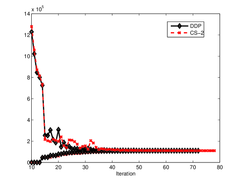
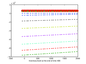
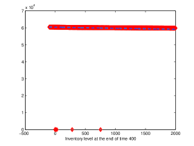
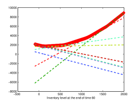
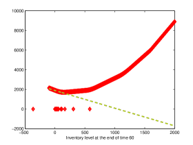
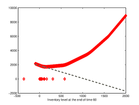
We report in Table 1 the corresponding computational time and approximate optimal value obtained with each algorithm. For DDP, DDP-CS-1, and DDP-CS-2, we additionally report the number of iterations of the algorithm. We see that on this instance, up to the precision $\varepsilon$, all algorithms provide the same approximate optimal value. Simplex is the quickest, DP is by far the slowest, and DDP and its variants are in between, with DDP-CS-1 and DDP-CS-2 variants requiring more iterations than DDP without cut selection to converge. Though DDP-CS-1 and DDP-CS-2 run for the same number of iterations, DDP-CS-2 is quicker than DDP-CS-1 (and than DDP too), due to the fact that for many iterations and stages it selects much less cuts than DDP-CS-1. More precisely, DDP-CS-2 is 13.7% quicker than DDP and 20.4% quicker than DDP-CS-1. As an illustration, we plot on Figure 3 approximations of value functions $\mathcal{Q}_{t}(y_{t})$ for step $t=401$ estimated using DP and the cuts for these functions obtained at the last iteration of DDP, DDP-CS-1, and DDP-CS-2. Surprisingly, DDP-CS-2 only selected one cut at the last iteration. For DDP-CS-1, we observe that though 44 cuts are selected, they are all equal. This explains why graphically, we obtain on Figure 3 the same cuts for DDP-CS-1 and DDP-CS-2 for $t=401$. Moreover, looking at Figure 3, we see that for $t=400$, the cuts built by DDP have similar slopes and many of these cuts are useless, i.e., they are below the approximate cost-to-go function on the interval $[-100,2000]$. This explains why so many cuts are pruned.

Similar conclusions were drawn taking $T=96$ and several values of $t$, see Figure 3 for $T=96$ and $t=61$. For this experiment ($T=96$), at the last iteration, for $t=61$ DDP-CS-2 only selects one cut and DDP 17 cuts (the number of iterations). Surprisingly again, not only does DDP-CS-1 select more cuts (6 for $t=61$) but all these cuts are identical.

Algorithm	Computational time	Iterations	Optimal value
Simplex	0.0868	-	110 660
DP	20 623	-	110 660
DDP	76.0214	72	110 660
DDP-CS-2	65.6318	78	110 660
DDP-CS-1	82.4705	78	110 660

Table 1. Computational time (in seconds) and approximate optimal values solving an instance of (7.31) with Simplex, DP, DDP, DDP-CS-1, and DDP-CS-2 with $T=600,N=2001$, and $\varepsilon=0.1$.

Figure 3. Approximate value functions $\mathcal{Q}_{t}(y_{t})$ estimated using DP (solid lines) and cuts for these functions (dashed lines) obtained at the last iteration of DDP, DDP-CS-1, and DDP-CS-2. Top left: $t=401,T=600$, DDP. Top right: $t=401,T=600$, DDP-CS-1. Middle left: $t=401,T=600$, DDP-CS-2. Middle right: $t=61,T=96$, DDP. Bottom left: $t=61,T=96$, DDP-CS-1. Bottom right: $t=61,T=96$, DDP-CS-2. Trial points less than $2000$ are represented by diamond markers on the $x$-axis.

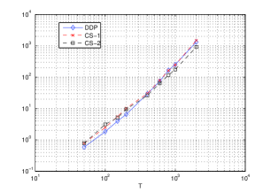
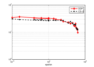
Finally, for DDP and its variants, we report in Figure 4 the log-log evolution of the computational time for DDP and its variants as a function of the number of steps $T$ (fixing $\varepsilon=0.1$) running the algorithms for $T$ in the set $\{50,100,150,200,400,600,800,1000,5000\}$. We observe that for sufficiently large values of $T$, DDP-CS-2 is the quickest. On this figure, we also report the log-log evolution of the computational time as a function of $\varepsilon$ taking $\varepsilon$ in the set $\{0.00001,0.0001,0.001,0.01,0.1,1,5,10,50,100,500$, $1\,000,2\,000,3\,000,4\,000,5\,000,6\,000,7\,000,8\,000$,
$9\,000,10\,061\}$ and fixing $T=400$ for DDP and DDP-CS-2 (the last value $10\,061$ of $\varepsilon$ taken corresponds to 25% of the optimal value of the problem). We see that unless $\varepsilon$ is very large, the computational time slowly decreases with $\varepsilon$.

Figure 4. Computational time (in seconds) as a function of $T$ and $\varepsilon$ for DDP and its variants DDP-CS-1 and DDP-CS-2 (CS-1 and CS-2 for short)

.

7.2. A portfolio problem

Consider the portfolio problem with known returns

(7.32) $$\begin{array}[]{l}\max\;\sum\limits_{i=1}^{n+1}(1+r^{i}_{T})x^{i}_{T}\\ x^{i}_{t}=(1+r_{t-1}^{i})x_{t-1}^{i}-y_{t}^{i}+z_{t}^{i},\;i=1,\ldots,n,\;t=1,\ldots,T,\\ x_{t}^{n+1}=(1+r_{t-1}^{n+1})x_{t-1}^{n+1}+\sum\limits_{i=1}^{n}(1-\eta_{i})y_{t}^{i}-\sum\limits_{i=1}^{n}(1+\nu_{i})z_{t}^{i},\;t=1,\ldots,T,\\ x_{t}^{i}\leq u_{i}\sum\limits_{i=1}^{n+1}(1+r_{t-1}^{i})x_{t-1}^{i},\;i=1,\ldots,n,\;t=1,\ldots,T,\\ x_{t}^{i}\geq 0,\;i=1,\ldots,n+1,\;t=1,\ldots,T,\\ y_{t}^{i}\geq 0,z_{t}^{i}\geq 0,\;i=1,\ldots,n,\;t=1,\ldots,T.\end{array}$$

Here $n$ is the number of assets, asset $n+1$ is cash, $T$ is the number of time periods, $x_{t}^{i}$ is the value of asset $i=1,\ldots,n+1$ at the beginning of time period $t=1,\ldots,T$, $r_{t}^{i}$ is the return of asset $i$ for period $t$, $y_{t}^{i}$ is the amount of asset $i$ sold at time $t$, $z_{t}^{i}$ is the amount of asset $i$ bought at time $t$, $\eta_{i}>0$ and $\nu_{i}>0$ are the respective transaction costs. The components $x_{0}^{i},i=1,\ldots,n+1$ are drawn independently of each other from the uniform distribution over the interval $[0,100]$ ($x_{0}$ is the initial portfolio). The expression $\sum\limits_{i=1}^{n+1}(1+r_{t-1}^{i})x_{t-1}^{i}$ is the budget available at the beginning of period $t$. The notation $u_{i}$ in the third group of constraints is a parameter defining the maximal proportion that can be invested in financial security $i$.

We take $u_{i}=1$ for all $i$, and define several instances of (7.32) with $T=90$ and $n$ (the size of state vector $x_{t}$ in (3.5)) $\in$ $\{2,3,5,8,10,15,20,25,30,35,40$, $45,50,60,70,80$, $90,100,120,140,160,180$,
$200,300,400,500,600,700,800,900,1000,1500\}$. The returns of assets $i=1,\ldots,n$, are drawn independently of each other from the uniform distribution over the interval $[0.00005,0.0004]$, the return of asset $n+1$ is fixed to $0.0001$ (assuming daily returns, this amounts to a 3.72% return over 365 days), and transaction costs $\nu_{i},\mu_{i}$ are set to $0.001$.

In the notation of the previous section, these instances are solved using Simplex, DDP, DDP-CS-1, and DDP-CS-2. Since we consider in this section problems and state vectors of large size (state vector size up to $1500$ and problems with up to 405 090 variables and up to 675 090 constraints [including box constraints]), DP leads to prohibitive computational times and is not used. The computational time required to solve these instances is reported in Table 2 (all implementations are in Matlab, using Mosek Optimization Toolbox [1] and for all algorithms the computational time includes the time to fill the constraint matrices). For DDP and its variants, we take $\varepsilon=1$. To check the implementation, we report in the Appendix, in Table 6, the approximate optimal values obtained for these instances with all algorithms. We observe that Simplex tends to be quicker on small instances but when the state vector is large, DDP and its variants are much quicker. The variants with and without cut selection have similar performances on most instances with DDP-CS-1 and DDP-CS-2 tending to be quicker for the instances with large $n$ (for instance for DDP-CS-2 compared to DDP: 18 seconds instead of 21 seconds for $(T,n)=(90,1500)$).

If the DDP algorithms are very efficient, the variants with cut selection have not yielded a significant reduction in computational time on these instances. This can be partly explained by the small number of iterations (at most 5) needed for DDP algorithms to converge on these runs.

$n$	2	3	5	8	10	15	20	25
Simplex	0.0847	0.0246	0.0413	0.0786	0.1070	0.2685	0.3831	0.6089
DDP	0.2314	0.2440	0.4721	0.2845	0.5880	0.7401	0.6886	0.7738
DDP-CS-2	0.2652	0.2626	0.5021	0.3018	0.6129	0.6651	0.7079	0.7800
DDP-CS-1	0.2480	0.2630	0.5372	0.3105	0.6227	0.6888	0.7821	0.791
$n$	30	35	40	45	50	60	70	80
Simplex	0.9670	1.3484	1.5092	1.9607	2.5572	3.5763	5.5887	7.2446
DDP	0.7735	0.7906	0.8337	0.8501	0.9177	0.9733	1.0739	1.1434
DDP-CS-2	0.8045	0.8198	0.8676	0.8771	0.9520	1.0036	1.1068	1.1766
DDP-CS-1	0.8056	0.8267	0.8788	0.8816	0.9545	1.0094	1.1103	1.1795
$n$	90	100	120	140	160	180	200	300
Simplex	8.5491	12.1851	25.7598	36.5120	38.4824	46.0557	72.2004	129.2468
DDP	1.1687	1.3347	1.4285	1.5798	1.7350	1.8178	2.0015	2.9424
DDP-CS-2	1.1833	1.3600	1.4464	1.5713	1.7479	1.8459	2.0315	2.9600
DDP-CS-1	1.1909	1.3571	1.4459	1.5728	1.7509	1.8488	2.0413	2.9551
$n$	400	500	600	700	800	900	1000	1500
Simplex	263.4561	509.4387	765.1	1084.8	1568	2080.9	2922	10 449
DDP	3.8153	5.7445	7.5	8.8	9.0	10.0	11	21
DDP-CS-2	3.8197	5.7206	7.4	8.6	8.9	10.0	11	18
DDP-CS-1	3.8319	5.7955	7.4	8.7	9.0	10.1	11	18

Table 2. Computational time (in seconds) to solve instances of (7.32) with Simplex, DDP, DDP-CS-1, and DDP-CS-2 for $T=90$ and several values of $n$.

Finally, we apply Simplex, DDP, DDP-CS-1, and DDP-CS-2 algorithms on a portfolio problem of form (7.32) using daily historical returns of $n$ assets of the S&P 500 index for a period of $T$ days starting on January 4, 2010, assuming these returns known (which provides us with the maximal possible return over this period using these assets). We consider 8 combinations for the pair $(T,n)$: $(25,50)$, $(50,50)$, $(75,50)$, $(100,50)$, $(25,100)$, $(50,100)$, $(75,100)$, and $(100,100)$. We take again $\nu_{i}=\mu_{i}=0.001$ and $u_{i}=1$ for all $i$. The components $x_{0}^{i},i=1,\ldots,n+1$ of $x_{0}$ are drawn independently of each other from the uniform distribution over the interval $[0,100]$. The return of asset $n+1$ is $0.001$ for all steps.

For this experiment, we report the computational time and the approximate optimal values in respectively Tables 3 and 4. Again the DDP variants are much quicker than simplex for problems with large $T,n$. The variants with cut selection are quicker, especially when $T$ and $n$ are large (compared to DDP, DDP-CS-2 is 5% quicker for $(T,n)=(75,100)$ and 6% quicker for $(T,n)=(100,100)$). The number of iterations needed for the DDP variants to converge is given in Table 5.

$(T,n)$	$(25,50)$	$(50,50)$	$(75,50)$	$(100,50)$	$(25,100)$	$(50,100)$	$(75,100)$	$(100,100)$
Simplex	0.5642	1.2783	1.9757	2.6020	2.6305	8.3588	9.2925	12.1430
DDP	0.3386	0.8705	1.6381	3.2622	1.2789	2.7525	6.0626	8.3887
DDP-CS-2	0.3207	0.8138	1.2053	2.8012	1.2520	2.2616	5.7634	7.8885
DDP-CS-1	0.3206	0.8036	1.2022	2.8261	1.2670	2.2801	5.8442	9.1096

Table 3. Computational time (in seconds) to solve instances of (7.32) with Simplex, DDP, DDP-CS-1, and DDP-CS-2 for several values of $(T,n)$ using historical returns of $n$ assets of S&P 500 index.

$(T,n)$	$(25,50)$	$(50,50)$	$(75,50)$	$(100,50)$	$(25,100)$	$(50,100)$	$(75,100)$	$(100,100)$
Simplex	4 754.3	10 600	24 525	46 496	13 584	53 576	178 190	403 800
DDP	4 754.2	10 600	24 525	46 496	13 584	53 576	178 190	403 800
DDP-CS-2	4 754.2	10 600	24 525	46 496	13 584	53 576	178 190	403 800
DDP-CS-1	4 754.2	10 600	24 525	46 496	13 584	53 576	178 190	403 800

Table 4. Approximate optimal value of instances of (7.32) obtained with Simplex, DDP, DDP-CS-1, and DDP-CS-2 for several values of $(T,n)$ using historical returns of $n$ assets of S&P 500 index.

$(T,n)$	$(25,50)$	$(50,50)$	$(75,50)$	$(100,50)$	$(25,100)$	$(50,100)$	$(75,100)$	$(100,100)$
DDP	6	7	7	11	12	13	17	17
DDP-CS-2	5	6	6	10	13	12	20	23
DDP-CS-1	5	6	6	10	13	12	20	20

Table 5. Number of iterations of DDP method with DDP, DDP-CS-1, and DDP-CS-2 for instances of (7.32) built using historical returns of $n$ assets of S&P 500 index.

8. Conclusion

We proved the convergence of DDP with cut selection for cut selection strategies satisfying Assumption (H2). This assumption is satisfied by the Territory algorithm [10], the Level $H$ cut selection [12], as well as the limited memory variant we proposed.

Numerical simulations on an inventory and a portfolio problem have shown that DDP can be much quicker than simplex and that cut selection can speed up the convergence of DDP for some large scale instances. For instance, for the simulated portfolio problem with $(T,n)=(90,1500)$ of Section 7, DDP was about 500 times quicker than simplex. We also recall that for the inventory problem solved for $T=600$, DDP-CS-2 (that uses the limited memory variant) was 13.7% quicker than DDP and 20.4% quicker than DDP-CS-1. A possible explanation is that DDP produced a large number of dominated/useless cuts, which are below the useful cuts on the whole range of admissible states. We expect more generally the cut selection strategies to be helpful when the number of iterations of DDP (and thus the number of cuts built) is large.

For the porfolio management instances with large $n$, DDP-CS-1 and DDP-CS-2 tend to be quicker (for the tests using historical daily returns of S&P 500 index, compared to DDP, DDP-CS-2 is 5% quicker for $(T,n)=(75,100)$ and 6% quicker for $(T,n)=(100,100)$).

The proof of this paper can be extended in several ways:

• As in [4], we can consider the case where $f_{t}$ and the constraint set for step $t$ depend not only on $x_{t-1}$ but on the full history of decisions $x_{1},x_{2},\ldots,x_{t-1}$. In this case, $\mathcal{Q}_{t}$ also depends on the full history of decisions $x_{1},x_{2},\ldots,x_{t-1}$. This larger problem class was considered for risk-averse convex programs without cut selection in [4].

• It is also possible to consider a variant of DDP that uses a backward pass to compute the cuts, i.e., that computes the cuts using at iteration $k$ function $\mathcal{Q}_{t+1}^{k}$ instead of $\mathcal{Q}_{t+1}^{k-1}$ in (4.7). The corresponding convergence proof can be easily obtained following the convergence proof of Theorem 5.2.

• Extend the convergence proof for decomposition methods with cut selection to solve multistage risk-averse nonlinear stochastic optimization problems.

Appendix

$n$	2	3	5	8	10	15	20	25
Simplex	63.9523	265.7561	300.7989	527.9508	515.5728	649.9466	1 156	1 138.4
DDP	63.9314	265.6687	300.7989	527.9489	515.5728	649.8515	1 156	1 138.4
DDP-CS-2	63.9314	265.6687	300.7989	527.9489	515.5728	649.8515	1 156	1 138.4
DDP-CS-1	63.9314	265.6687	300.7989	527.9489	515.5728	649.8515	1 156	1 138.4
$n$	30	35	40	45	50	60	70	80
Simplex	1 620.3	1 877.8	2 127.4	2 037.0	2 183.4	2 894.3	3 420.6	4 101.5
DDP	1 620.3	1 877.8	2 127.4	2 037.0	2 183.4	2 894.3	3 420.6	4 101.5
DDP-CS-2	1 620.3	1 877.8	2 127.4	2 037.0	2 183.4	2 894.3	3 420.6	4 101.5
DDP-CS-1	1 620.3	1 877.8	2 127.4	2 037.0	2 183.4	2 894.3	3 420.6	4 101.5
$n$	90	100	120	140	160	180	200	300
Simplex	4 919	5 147	6 306	6 835	8 254	9 151	9 773	16 016
DDP	4 919	5 147	6 306	6 835	8 254	9 151	9 773	16 016
DDP-CS-2	4 919	5 147	6 306	6 835	8 254	9 151	9 773	16 016
DDP-CS-1	4 919	5 147	6 306	6 835	8 254	9 151	9 773	16 016
$n$	400	500	600	700	800	900	1000	1500
Simplex	21 050	25 863	30 410	36 229	41 145	45 024	50 994	76 695
DDP	21 050	25 863	30 410	36 229	41 145	45 024	50 994	76 695
DDP-CS-2	21 050	25 863	30 410	36 229	41 145	45 024	50 994	76 695
DDP-CS-1	21 050	25 863	30 410	36 229	41 145	45 024	50 994	76 695

Table 6. Optimal values of instances of (7.32) considered in Section 7.2 solved with Simplex, DDP, DDP-CS-1, and DDP-CS-2 for $T=90$ and several values of $n$.

References

- [1] E. D. Andersen and K. D. Andersen. The MOSEK optimization toolbox for MATLAB manual. Version 7.0, 2013. http://docs.mosek.com/7.0/toolbox/.
- [2] S. Gaubert, W. McEneaney, and Z. Qu. Curse of dimensionality reduction in max-plus based approximation methods: Theoretical estimates and improved pruning algorithms. 50th IEEE Conference on Decision and Control and European Control Conference (CDC-ECC), pages 1054–1061, 2011.
- [3] V. Guigues. SDDP for some interstage dependent risk-averse problems and application to hydro-thermal planning. Computational Optimization and Applications, 57:167–203, 2014.
- [4] V. Guigues. Convergence analysis of sampling-based decomposition methods for risk-averse multistage stochastic convex programs. Accepted for publication in Siam Journal on Optimization, available on arXiv at http://arxiv.org/abs/1408.4439, 2016.
- [5] V. Guigues and W. Römisch. Sampling-based decomposition methods for multistage stochastic programs based on extended polyhedral risk measures. SIAM Journal on Optimization, 22:286–312, 2012.
- [6] V. Guigues and W. Römisch. SDDP for multistage stochastic linear programs based on spectral risk measures. Operations Research Letters, 40:313–318, 2012.
- [7] V. Kozmik and D.P. Morton. Evaluating policies in risk-averse multi-stage stochastic programming. Mathematical Programming, 152:275–300, 2015.
- [8] W.M. McEneaney, A. Deshpande, and S. Gaubert. Curse of complexity attenuation in the curse of dimensionality free method for HJB PDEs. American Control Conference, pages 4684–4690, 2008.
- [9] M.V.F. Pereira and L.M.V.G Pinto. Multi-stage stochastic optimization applied to energy planning. Mathematical Programming, 52:359–375, 1991.
- [10] Laurent Pfeiffer, Romain Apparigliato, and Sophie Auchapt. Two methods of pruning benders’ cuts and their application to the management of a gas portfolio. Research Report RR-8133, hal-00753578, 2012.
- [11] A. Philpott and V. de Matos. Dynamic sampling algorithms for multi-stage stochastic programs with risk aversion. European Journal of Operational Research, 218:470–483, 2012.
- [12] A. Philpott, V. de Matos, and E. Finardi. Improving the performance of stochastic dual dynamic programming. Journal of Computational and Applied Mathematics, 290:196–208, 2012.
- [13] A. B. Philpott and Z. Guan. On the convergence of stochastic dual dynamic programming and related methods. Operations Research Letters, 36:450–455, 2008.
- [14] A. Ruszczyński. Parallel decomposition of multistage stochastic programming problems. Math. Programming, 58:201–228, 1993.
- [15] A. Shapiro. Analysis of stochastic dual dynamic programming method. European Journal of Operational Research, 209:63–72, 2011.
- [16] A. Shapiro, D. Dentcheva, and A. Ruszczyński. Lectures on Stochastic Programming: Modeling and Theory. SIAM, Philadelphia, 2009.
- [17] A. Shapiro, W. Tekaya, J.P. da Costa, and M.P. Soares. Worst-case-expectation approach to optimization under uncertainty. Operations Research, 61:1435–1449, 2013.