Polarized Sunyaev Zel’dovich tomography

Anne-Sylvie Deutsch    Matthew C. Johnson    Moritz Münchmeyer    Alexandra Terrana
Abstract

Secondary CMB polarization is induced by the late-time scattering of CMB photons by free electrons on our past light cone. This polarized Sunyaev Zel’dovich (pSZ) effect is sensitive to the electrons’ locally observed CMB quadrupole, which is sourced primarily by long wavelength inhomogeneities. By combining the remote quadrupoles measured by free electrons throughout the Universe after reionization, the pSZ effect allows us to obtain additional information about large scale modes beyond what can be learned from our own last scattering surface. Here we determine the power of pSZ tomography, in which the pSZ effect is cross-correlated with the density field binned at several redshifts, to provide information about the long wavelength Universe. The signal we explore here is a power asymmetry in the cross-correlation between E𝐸E or B𝐵B mode CMB polarization and the density field. We compare this to the cosmic variance limited noise: the random chance to get a power asymmetry in the absence of a large scale quadrupole field. By computing the necessary transfer functions and cross-correlations, we compute the signal-to-noise ratio attainable by idealized next generation CMB experiments and galaxy surveys. We find that a signal-to-noise ratio of 110similar-toabsent110\sim 1-10 is in principle attainable over a significant range of power multipoles, with the strongest signal coming from the first multipoles in the lowest redshift bins. These results prompt further assessment of realistically measuring the pSZ signal and the potential impact for constraining cosmology on large scales.

1 Introduction

The direct observation of the primary cosmic microwave background (CMB) anisotropies has driven the era of precision cosmology, casting light on the contents and evolution of the Universe, and providing compelling evidence for the standard cosmological model, ΛΛ\LambdaCDM. The hunt for beyond-the-standard-cosmological-model (BSCM) physics has been ongoing, with the WMAP [1] and Planck [2] CMB satellites providing a few tantalizing clues for BSCM physics on the largest observable scales. These include a lack of correlations on large scales, the low CMB quadrupole power, the alignment of the temperature quadrupole and octupole, the Cold Spot, a hemispherical power asymmetry, and other anomalies (for a recent review see ref. [3]). Unfortunately, the statistical significance of such large scale anomalies cannot be assessed further using temperature anisotropies alone because the statistical and systematic errors in existing measurements are dominated by cosmic variance 111If the large-angle CMB polarization can be faithfully extracted from foregrounds, there will be some progress. .

However, there is another promising avenue to explore in the coming era of precision measurements of the secondary CMB, which is dominated by lensing and the Sunyaev Zel’dovich effect 222Here, we consider only the nearly frequency independent contributions, assuming that strongly frequency independent contributions such as the thermal Sunyaev Zel’dovich effect and the cosmic infrared background have been perfectly removed.. The scattering of photons onto our light-cone allows us to access additional realizations of the longest modes probed by the CMB, as the scattered photons originate from the bulk, and therefore carry information about modes inside our light-cone. Extracting this information could decrease the cosmic variance error on the largest modes, possibly alleviating (or confirming!) large scale anomalies. Two promising avenues include CMB lensing, which can be used to reconstruct our fundamental dipole [4], and the kinetic Sunyaev Zel’dovich effect [5, 6, 7, 8]. However, in this paper, we focus on the ability of the polarized Sunyaev-Zel’dovich (pSZ) effect [9, 10, 11, 12, 13, 14, 15], the induced CMB polarization due to Thomson scattering from free electrons after reionization, to provide constraints on large scale modes.

Thomson scattering of photons on a free electron creates a linear polarization pattern that depends on the quadrupole observed by the electron. Therefore, CMB polarization could be used to reconstruct distant quadrupoles, possibly yielding information about the large scale Universe. This idea, first proposed in ref. [16], has received significant attention in the literature. Previous work has explored the detectability of this effect based on the observation of CMB polarization in the direction of galaxy clusters [10, 17, 12], suggesting that the pSZ effect could be a target for the next generation of CMB experiments. The degree to which the pSZ effect gives constraints on primordial, large scale modes has been explored in refs. [18, 19, 20, 21, 22]. One important point is that the local quadrupole for different clusters are correlated with each other [23], making it important to assess the degree to which cosmic variance is in fact alleviated [20]. Because tensors contribute to the quadrupole, the pSZ effect has been proposed as a probe of primordial gravitational waves [15]. Finally, remote quadrupole measurements could have other implications for determining the properties of dark energy [24, 25] and the intra-cluster medium [26].

In this paper, we lay the theoretical foundation for pSZ tomography, the cross-correlation of CMB polarization arising from the pSZ effect with probes of large scale structure at different redshifts. This cross-correlation has an intrinsically statistically anisotropic component – a power asymmetry – which encodes the variation of the locally observed quadrupole along our past light cone. Performing this cross-correlation at different redshifts allows one to obtain three-dimensional information about the structure of the Universe on very large scales. More precisely, the contribution to the CMB polarization from the pSZ effect is proportional to qeff(1+δe)subscript𝑞eff1subscript𝛿𝑒q_{\rm eff}(1+\delta_{e}), where qeffsubscript𝑞effq_{\rm eff} is the remote quadrupole field, and δesubscript𝛿𝑒\delta_{e} is the electron density field. The cross-correlation with δesubscript𝛿𝑒\delta_{e} at different redshifts has a statistically anisotropic component (Q±iU)δeqeffδeδesimilar-todelimited-⟨⟩plus-or-minus𝑄𝑖𝑈subscript𝛿𝑒subscript𝑞effdelimited-⟨⟩subscript𝛿𝑒subscript𝛿𝑒\langle(Q\pm iU)\delta_{e}\rangle\sim q_{\rm eff}\langle\delta_{e}\delta_{e}\rangle, which is a long-wavelength modulation of small-scale power. In this paper, we characterize this signal by exploiting a decomposition of the Stokes parameters into curl-free E𝐸E modes and curl B𝐵B-modes and performing a multipolar decomposition of the cross-power as a function of redshift.

Measurements of the CMB polarization in the direction of galaxy clusters can be thought of as a special case of pSZ tomography, which focuses on the largest amplitude pixels in a pSZ map. However, the distribution of free electrons is a continuous field, implying that in principle there is more information to gather (this point was also highlighted in ref. [15]). One main result of this paper is to determine how much information there is to gather about the remote quadrupole field from the power asymmetry in the cosmic variance limit. Another result is to forecast the requirements for next generation of CMB experiments and galaxy surveys to measure the remote quadrupole field. An important further step is to connect the information that can be gathered from the remote quadrupole field to CMB anomalies and constraints on cosmological parameters. We pursue this question in future work.

The paper is organized as follows. Section 2 is devoted to the pSZ effect, where we derive the pSZ signal and its power spectrum. In section 3, we cross-correlate the pSZ signal with tracers of electron density at known redshift in order to find the pSZ tomography signal and its cosmic variance. In section 4 we discuss the detectability of the signal. We present our conclusions in section 5. A number of calculations are collected in a set of appendices.

2 The polarized SZ effect

Unpolarized light incident on free electrons becomes polarized due to Thomson scattering. The polarization generated depends on the quadrupole observed by the free electron. The polarized SZ (pSZ) effect can therefore be thought of as a census of the remote quadrupole as observed by free electrons on our past light cone. The contribution to the Stokes parameters Q±iUplus-or-minus𝑄𝑖𝑈Q\pm iU is given by an integral along the line of sight as

(Q±iU)pSZ(𝐧^e)=610𝑑χedτ(𝐧^e,χe)dχeeτ(𝐧^e,χe)m=22qeffm(𝐧^e,χe)Y2m±2(𝐧^e).superscriptplus-or-minus𝑄𝑖𝑈pSZsubscript^𝐧𝑒610differential-dsubscript𝜒𝑒𝑑𝜏subscript^𝐧𝑒subscript𝜒𝑒𝑑subscript𝜒𝑒superscript𝑒𝜏subscript^𝐧𝑒subscript𝜒𝑒superscriptsubscript𝑚22subscriptsuperscript𝑞𝑚effsubscript^𝐧𝑒subscript𝜒𝑒subscriptsubscript𝑌2𝑚plus-or-minus2subscript^𝐧𝑒(Q\pm iU)^{\text{pSZ}}({\bf\hat{n}}_{e})=-\frac{\sqrt{6}}{10}\int d\chi_{e}\frac{d\tau({\bf\hat{n}}_{e},\chi_{e})}{d\chi_{e}}\ e^{-\tau({\bf\hat{n}}_{e},\chi_{e})}\sum_{m=-2}^{2}q^{m}_{\rm eff}({\bf\hat{n}}_{e},\chi_{e})\left.{}_{\pm 2}Y_{2m}\right.({\bf\hat{n}}_{e}). (2.1)

Here, the optical depth τ𝜏\tau is defined by,

τ(𝐧^e,χe)=0χe𝑑χσTaene(𝐧^e,χ),dτ(𝐧^e,χe)dχe=σTaene(𝐧^e,χe),formulae-sequence𝜏subscript^𝐧𝑒subscript𝜒𝑒superscriptsubscript0subscript𝜒𝑒differential-d𝜒subscript𝜎𝑇subscript𝑎𝑒subscript𝑛𝑒subscript^𝐧𝑒𝜒𝑑𝜏subscript^𝐧𝑒subscript𝜒𝑒𝑑subscript𝜒𝑒subscript𝜎𝑇subscript𝑎𝑒subscript𝑛𝑒subscript^𝐧𝑒subscript𝜒𝑒\tau({\bf\hat{n}}_{e},\chi_{e})=\int_{0}^{\chi_{e}}d\chi\ \sigma_{T}a_{e}n_{e}({\bf\hat{n}}_{e},\chi),\ \ \ \frac{d\tau({\bf\hat{n}}_{e},\chi_{e})}{d\chi_{e}}=\sigma_{T}a_{e}n_{e}({\bf\hat{n}}_{e},\chi_{e}), (2.2)

where σTsubscript𝜎𝑇\sigma_{T} is the Thomson cross-section, ne(𝐧^e,χe)subscript𝑛𝑒subscript^𝐧𝑒subscript𝜒𝑒n_{e}({\bf\hat{n}}_{e},\chi_{e}) is the electron number density, 𝐧^esubscript^𝐧𝑒{\bf\hat{n}}_{e} denotes the angular direction to the free electron on the sky, and χesubscript𝜒𝑒\chi_{e} is the comoving radial coordinate to the electron along our past light cone,

χe=0zedzH(z)=1aedaH(a)a2,subscript𝜒𝑒superscriptsubscript0subscript𝑧𝑒𝑑𝑧𝐻𝑧superscriptsubscript1subscript𝑎𝑒𝑑𝑎𝐻𝑎superscript𝑎2\chi_{e}=\int_{0}^{z_{e}}\frac{dz}{H(z)}=-\int_{1}^{a_{e}}\ \frac{da}{H(a)a^{2}}, (2.3)

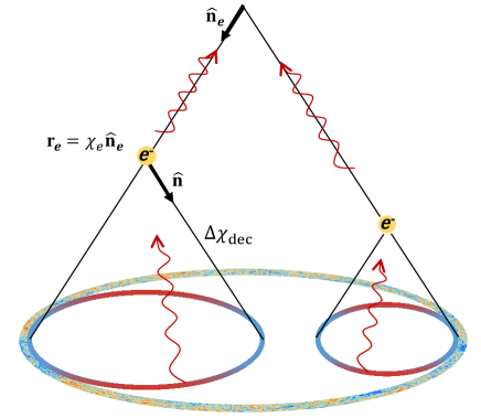
where zesubscript𝑧𝑒z_{e} and aesubscript𝑎𝑒a_{e} are the electron’s redshift and scale factor respectively. Figure 1 describes the geometry.
Refer to caption
Figure 1: CMB photons scattering off free electrons on our past light cone. An electron’s position is given by 𝐫e=χe𝐧^esubscript𝐫𝑒subscript𝜒𝑒subscript^𝐧𝑒{\bf r}_{e}=\chi_{e}{\bf\hat{n}}_{e}. From the electron’s location, the direction to a point on its surface of last scattering is 𝐧^^𝐧{\bf\hat{n}} and the distance to last scattering is ΔχdecΔsubscript𝜒dec\Delta\chi_{\text{dec}}. Notice that the scattering provides information about CMB photons from inside our past light cone. Specifically, the pSZ effect is sensitive to the locally observed quadrupole.

Well after reionization, we can approximate by substituting eq. (2.2) into eq. (2.1), obtaining

(Q±iU)pSZ(𝐧^e)=superscriptplus-or-minus𝑄𝑖𝑈pSZsubscript^𝐧𝑒absent\displaystyle(Q\pm iU)^{\text{pSZ}}({\bf\hat{n}}_{e})= 6σT10𝑑χeaen¯e(χe)(1+δe(𝐧^e,χe))6subscript𝜎𝑇10differential-dsubscript𝜒𝑒subscript𝑎𝑒subscript¯𝑛𝑒subscript𝜒𝑒1subscript𝛿𝑒subscript^𝐧𝑒subscript𝜒𝑒\displaystyle-\frac{\sqrt{6}\ \sigma_{T}}{10}\int d\chi_{e}\ a_{e}\bar{n}_{e}(\chi_{e})(1+\delta_{e}({\bf\hat{n}}_{e},\chi_{e})) (2.4)
×m=22qeffm(𝐧^e,χe)Y2m±2(𝐧^e),\displaystyle\qquad\times\sum_{m=-2}^{2}q^{m}_{\rm eff}({\bf\hat{n}}_{e},\chi_{e})\left.{}_{\pm 2}Y_{2m}\right.({\bf\hat{n}}_{e}), (2.5)

where we have written the electron number density as ne(𝐧^e,χe)=n¯e(χe)(1+δe(𝐧^e,χe))subscript𝑛𝑒subscript^𝐧𝑒subscript𝜒𝑒subscript¯𝑛𝑒subscript𝜒𝑒1subscript𝛿𝑒subscript^𝐧𝑒subscript𝜒𝑒n_{e}({\bf\hat{n}}_{e},\chi_{e})=\bar{n}_{e}(\chi_{e})(1+\delta_{e}({\bf\hat{n}}_{e},\chi_{e})) in terms of the average electron number density n¯e(χe)subscript¯𝑛𝑒subscript𝜒𝑒\bar{n}_{e}(\chi_{e}), and the density contrast δesubscript𝛿𝑒\delta_{e}. From here on, we will assume that electrons trace dark matter, and therefore we use δ𝛿\delta rather than δesubscript𝛿𝑒\delta_{e}. We make this assumption for simplicity, and this will not change the main results presented below. We defer a more accurate model for the electron distribution to future work.

The key quantity of interest, denoted by qeffm(𝐧^e,χe)subscriptsuperscript𝑞𝑚effsubscript^𝐧𝑒subscript𝜒𝑒q^{m}_{\rm eff}({\bf\hat{n}}_{e},\chi_{e}), is the CMB quadrupole observed by an electron along our past light cone in the 𝐧^esubscript^𝐧𝑒{\bf\hat{n}}_{e} direction at comoving distance χesubscript𝜒𝑒\chi_{e} (or alternatively, located at 𝐫e=χe𝐧^esubscript𝐫𝑒subscript𝜒𝑒subscript^𝐧𝑒{\bf r}_{e}=\chi_{e}{\bf\hat{n}}_{e}):

qeffm(𝐧^e,χe)=Ωd2𝐧^Θ(χe,𝐧^e,𝐧^)Y2m(𝐧^).subscriptsuperscript𝑞𝑚effsubscript^𝐧𝑒subscript𝜒𝑒subscriptΩsuperscript𝑑2^𝐧Θsubscript𝜒𝑒subscript^𝐧𝑒^𝐧subscriptsuperscript𝑌2𝑚^𝐧q^{m}_{\rm eff}({\bf\hat{n}}_{e},\chi_{e})=\int_{\Omega}d^{2}{\bf\hat{n}}\ \Theta(\chi_{e},{\bf\hat{n}}_{e},{\bf\hat{n}})\ Y^{*}_{2m}({\bf\hat{n}}). (2.6)

There are three contributions to the local CMB temperature at the position of the electron: the Sachs-Wolfe effect (SW) due to gravitational redshifting at the surface of last scattering, the integrated Sachs-Wolfe effect (ISW) resulting from the late-time evolution of gravitational potential, and the Doppler effect from the relative motion of electrons at the surface of last scattering and at an observer’s location. We can write each contribution in terms of the primordial Newtonian gravitational potential ΨisubscriptΨ𝑖\Psi_{i}:

ΘSW(𝐧^e,χe,𝐧^)=subscriptΘSWsubscript^𝐧𝑒subscript𝜒𝑒^𝐧absent\displaystyle\Theta_{\rm SW}({\bf\hat{n}}_{e},\chi_{e},{\bf\hat{n}})= (2DΨ(χdec)32)Ψi(𝐫dec),2subscript𝐷Ψsubscript𝜒dec32subscriptΨ𝑖subscript𝐫dec\displaystyle\left(2D_{\Psi}(\chi_{\text{dec}})-\frac{3}{2}\right)\Psi_{i}({\bf r}_{\text{dec}}), (2.7)
ΘISW(𝐧^e,χe,𝐧^)=subscriptΘISWsubscript^𝐧𝑒subscript𝜒𝑒^𝐧absent\displaystyle\Theta_{\rm ISW}({\bf\hat{n}}_{e},\chi_{e},{\bf\hat{n}})= 2adecaedDΨdaΨi(𝐫(a))𝑑a,2superscriptsubscriptsubscript𝑎decsubscript𝑎𝑒𝑑subscript𝐷Ψ𝑑𝑎subscriptΨ𝑖𝐫𝑎differential-d𝑎\displaystyle\ 2\int_{a_{\rm dec}}^{a_{e}}\frac{dD_{\Psi}}{da}\Psi_{i}({\bf r}(a))da, (2.8)
ΘDoppler(𝐧^e,χe,𝐧^)=subscriptΘDopplersubscript^𝐧𝑒subscript𝜒𝑒^𝐧absent\displaystyle\Theta_{\rm Doppler}({\bf\hat{n}}_{e},\chi_{e},{\bf\hat{n}})= 𝐧^[Dv(χdec)Ψi(𝐫dec)Dv(χe)Ψi(𝐫e)].^𝐧delimited-[]subscript𝐷𝑣subscript𝜒decsubscriptΨ𝑖subscript𝐫decsubscript𝐷𝑣subscript𝜒𝑒subscriptΨ𝑖subscript𝐫𝑒\displaystyle\ {\bf\hat{n}}\cdot\left[D_{v}(\chi_{\text{dec}})\nabla\Psi_{i}({\bf r}_{\text{dec}})-D_{v}(\chi_{e})\nabla\Psi_{i}({\bf r}_{e})\right]. (2.9)

In the above equations, we define the distance as 𝐫(a)χe𝐧^e+Δχ(a)𝐧^𝐫𝑎subscript𝜒𝑒subscript^𝐧𝑒Δ𝜒𝑎^𝐧{\bf r}(a)\equiv\chi_{e}{\bf\hat{n}}_{e}+\Delta\chi(a){\bf\hat{n}} with Δχ(a)=aea𝑑a[H(a)a2]1Δ𝜒𝑎superscriptsubscriptsubscript𝑎𝑒𝑎differential-dsuperscript𝑎superscriptdelimited-[]𝐻superscript𝑎superscript𝑎21\Delta\chi(a)=-\int_{a_{e}}^{a}da^{\prime}[H(a^{\prime})a^{\prime 2}]^{-1} (see figure 1). Specifically, 𝐫dec=𝐫(adec)subscript𝐫dec𝐫subscript𝑎dec{\bf r}_{\text{dec}}={\bf r}(a_{\text{dec}}) and Δχdec=Δχ(adec)Δsubscript𝜒decΔ𝜒subscript𝑎dec\Delta\chi_{\text{dec}}=\Delta\chi(a_{\text{dec}}), while the comoving distance to decoupling is simply χdec=1adec𝑑a[H(a)a2]1subscript𝜒decsuperscriptsubscript1subscript𝑎decdifferential-d𝑎superscriptdelimited-[]𝐻𝑎superscript𝑎21\chi_{\text{dec}}=-\int_{1}^{a_{\text{dec}}}da[H(a)a^{2}]^{-1}. We have introduced the growth function, DΨ(χ)subscript𝐷Ψ𝜒D_{\Psi}(\chi), which relates the potential to its primordial value at a0𝑎0a\rightarrow 0 through the definition

Ψ(𝐫,χ)=DΨ(χ)Ψi(𝐫).Ψ𝐫𝜒subscript𝐷Ψ𝜒subscriptΨ𝑖𝐫\Psi({\bf r},\chi)=D_{\Psi}(\chi)\Psi_{i}({\bf r}). (2.10)

On superhorizon scales, we can employ the approximation

DΨ(a)ΨSH(a)ΨSH,i=161+y+9y3+2y28y1610y3[52ΩmE(a)a0adaE3(a)a3],subscript𝐷Ψ𝑎subscriptΨSH𝑎subscriptΨSHi161𝑦9superscript𝑦32superscript𝑦28𝑦1610superscript𝑦3delimited-[]52subscriptΩ𝑚𝐸𝑎𝑎superscriptsubscript0𝑎𝑑𝑎superscript𝐸3𝑎superscript𝑎3D_{\Psi}(a)\equiv\frac{\Psi_{\rm SH}(a)}{\Psi_{\rm SH,i}}=\frac{16\sqrt{1+y}+9y^{3}+2y^{2}-8y-16}{10y^{3}}\left[\frac{5}{2}\Omega_{m}\frac{E(a)}{a}\int_{0}^{a}\frac{da}{E^{3}(a)\ a^{3}}\right], (2.11)

where ya/aeq𝑦𝑎subscript𝑎eqy\equiv a/a_{\text{eq}} and E(a)Ωma3+ΩΛ𝐸𝑎subscriptΩ𝑚superscript𝑎3subscriptΩΛE(a)\equiv\sqrt{\Omega_{m}a^{-3}+\Omega_{\Lambda}} is the normalized Hubble parameter. The velocity growth function Dvsubscript𝐷𝑣D_{v} in eq. (2.9), defined by 𝐯(𝐫,χ)=Dv(χ)Ψi(𝐫)𝐯𝐫𝜒subscript𝐷𝑣𝜒subscriptΨ𝑖𝐫{\bf v}({\bf r},\chi)=-D_{v}(\chi)\nabla\Psi_{i}({\bf r}), is given in terms of scale factor as,

Dv(a)2a2H(a)H02Ωmy4+3y[DΨ+dDΨdlna].subscript𝐷𝑣𝑎2superscript𝑎2𝐻𝑎subscriptsuperscript𝐻20subscriptΩ𝑚𝑦43𝑦delimited-[]subscript𝐷Ψ𝑑subscript𝐷Ψ𝑑𝑎D_{v}(a)\equiv\frac{2a^{2}H(a)}{H^{2}_{0}\Omega_{m}}\frac{y}{4+3y}\left[D_{\Psi}+\frac{dD_{\Psi}}{d\ln a}\right]. (2.12)

2.1 Fourier kernel for the effective quadrupole

In this subsection, we relate the effective quadrupole qeffmsubscriptsuperscript𝑞𝑚effq^{m}_{\rm eff} given in eq. (2.6) to the primordial gravitational potential, ΨisubscriptΨ𝑖\Psi_{i}, through the expressions given in (2.7)-(2.9). Firstly express ΨisubscriptΨ𝑖\Psi_{i} in Fourier space as

Ψi(𝐫)=d3k(2π)3Ψ~i(𝐤)eiχe𝐤𝐧^eeiΔχ𝐤𝐧^,subscriptΨ𝑖𝐫superscript𝑑3𝑘superscript2𝜋3subscript~Ψ𝑖𝐤superscript𝑒𝑖subscript𝜒𝑒𝐤subscript^𝐧𝑒superscript𝑒𝑖Δ𝜒𝐤^𝐧\Psi_{i}({\bf r})=\int\frac{d^{3}k}{(2\pi)^{3}}\tilde{\Psi}_{i}({\bf k})e^{i\chi_{e}{\bf k}\cdot{\bf\hat{n}}_{e}}e^{i\Delta\chi{\bf k}\cdot{\bf\hat{n}}}, (2.13)

where we have explicitly expanded the position 𝐫=χe𝐧^e+Δχ𝐧^𝐫subscript𝜒𝑒subscript^𝐧𝑒Δ𝜒^𝐧{\bf r}=\chi_{e}{\bf\hat{n}}_{e}+\Delta\chi{\bf\hat{n}}. Inserting the expressions for each contribution to the CMB temperature (2.7)-(2.9) in (2.6), we obtain (see Appendix A for the details of the calculation):

qeffm(𝐧^e,χe)=d3k(2π)3Ψ~i(𝐤)T(k)[𝒢SW+𝒢ISW+𝒢Doppler]Y2m(𝐤^)eiχe𝐤𝐧^e,subscriptsuperscript𝑞𝑚effsubscript^𝐧𝑒subscript𝜒𝑒superscript𝑑3𝑘superscript2𝜋3subscript~Ψ𝑖𝐤𝑇𝑘delimited-[]subscript𝒢SWsubscript𝒢ISWsubscript𝒢Dopplersuperscriptsubscript𝑌2𝑚^𝐤superscript𝑒𝑖subscript𝜒𝑒𝐤subscript^𝐧𝑒q^{m}_{\rm eff}({\bf\hat{n}}_{e},\chi_{e})=\int\frac{d^{3}k}{(2\pi)^{3}}\tilde{\Psi}_{i}({\bf k})T(k)\left[\mathcal{G}_{\rm SW}+\mathcal{G}_{\rm ISW}+\mathcal{G}_{\rm Doppler}\right]Y_{2m}^{*}({\bf\hat{k}})\ e^{i\chi_{e}{\bf k}\cdot{\bf\hat{n}}_{e}}, (2.14)

where the kernels 𝒢SWsubscript𝒢SW\mathcal{G}_{\rm SW}, 𝒢ISWsubscript𝒢ISW\mathcal{G}_{\rm ISW} and 𝒢Dopplersubscript𝒢Doppler\mathcal{G}_{\rm Doppler} are given by:

𝒢SW(k,χe)=subscript𝒢SW𝑘subscript𝜒𝑒absent\displaystyle\mathcal{G}_{\rm SW}(k,\chi_{e})= 4π(2DΨ(χdec)32)j2(kΔχdec),4𝜋2subscript𝐷Ψsubscript𝜒dec32subscript𝑗2𝑘Δsubscript𝜒dec\displaystyle-4\pi\left(2D_{\Psi}(\chi_{\rm dec})-\frac{3}{2}\right)j_{2}(k\Delta\chi_{\text{dec}}),
𝒢ISW(k,χe)=subscript𝒢ISW𝑘subscript𝜒𝑒absent\displaystyle\mathcal{G}_{\rm ISW}(k,\chi_{e})= 8πadecae𝑑adDΨdaj2(kΔχ(a)),8𝜋superscriptsubscriptsubscript𝑎decsubscript𝑎𝑒differential-d𝑎𝑑subscript𝐷Ψ𝑑𝑎subscript𝑗2𝑘Δ𝜒𝑎\displaystyle-8\pi\int_{a_{\rm dec}}^{a_{e}}da\frac{dD_{\Psi}}{da}\ j_{2}(k\Delta\chi(a)),
𝒢Doppler(k,χe)=subscript𝒢Doppler𝑘subscript𝜒𝑒absent\displaystyle\mathcal{G}_{\rm Doppler}(k,\chi_{e})= 4π5kDv(χdec)[3j3(kΔχdec)2j1(kΔχdec)].4𝜋5𝑘subscript𝐷𝑣subscript𝜒decdelimited-[]3subscript𝑗3𝑘Δsubscript𝜒dec2subscript𝑗1𝑘Δsubscript𝜒dec\displaystyle\frac{4\pi}{5}kD_{v}(\chi_{\text{dec}})\left[3j_{3}(k\Delta\chi_{\text{dec}})-2j_{1}(k\Delta\chi_{\text{dec}})\right]. (2.15)

We have also incorporated the transfer function, T(k)𝑇𝑘T(k), in the above expression which we approximate using the BBKS fitting function [27],

T(k)=ln[1+0.171x]0.171x[1+0.284x+(1.18x)2+(0.399x)3+(0.49x)4]0.25,𝑇𝑘10.171𝑥0.171𝑥superscriptdelimited-[]10.284𝑥superscript1.18𝑥2superscript0.399𝑥3superscript0.49𝑥40.25T(k)=\frac{\ln\left[1+0.171x\right]}{0.171x}\left[1+0.284x+(1.18x)^{2}+(0.399x)^{3}+(0.49x)^{4}\right]^{-0.25}\ , (2.16)

where x=k/keq𝑥𝑘subscript𝑘eqx=k/k_{\rm eq} with keq=aeqH(aeq)=2/aeqH082.5H0subscript𝑘eqsubscript𝑎eq𝐻subscript𝑎eq2subscript𝑎eqsubscript𝐻0similar-to-or-equals82.5subscript𝐻0k_{\rm eq}=a_{\rm eq}H(a_{\rm eq})=\sqrt{2/a_{\rm eq}}H_{0}\simeq 82.5H_{0}.

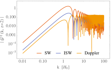
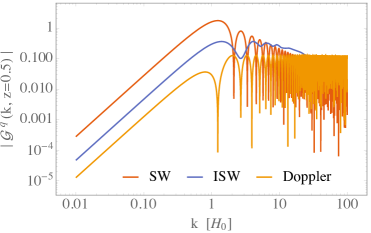
The kernels in eq. 2.15 are plotted in figure 2 at ze=0.5subscript𝑧𝑒0.5z_{e}=0.5 (left) and ze=2.0subscript𝑧𝑒2.0z_{e}=2.0 (right). The dominant contribution to the SW and ISW kernels are from large scales, with the amplitude peaking near kH0similar-to𝑘subscript𝐻0k\sim H_{0}. On large scales, the SW and Doppler contributions are negative, while the ISW contribution is positive. To leading order in k𝑘k, each kernel is proportional to k2superscript𝑘2k^{2} in the limit k0𝑘0k\rightarrow 0. Note that there is only a partial cancellation between the SW, Doppler and ISW contributions to the quadrupole field. On sufficiently small scales, k20H0greater-than-or-equivalent-to𝑘20subscript𝐻0k\gtrsim 20H_{0}, the Doppler contribution dominates the SW and ISW components of the quadrupole field. Finally, comparing the left and right panel of figure 2, the kernel is more sensitive to larger scales at lower redshifts (as expected from the geometry in Figure 1).
Refer to caption
Refer to caption
Figure 2: The three contributions to the kernel, 𝒢SW(k,χe)subscript𝒢SW𝑘subscript𝜒𝑒\mathcal{G}_{\rm SW}(k,\chi_{e}), 𝒢ISW(k,χe)subscript𝒢ISW𝑘subscript𝜒𝑒\mathcal{G}_{\rm ISW}(k,\chi_{e}), and 𝒢Doppler(k,χe)subscript𝒢Doppler𝑘subscript𝜒𝑒\mathcal{G}_{\rm Doppler}(k,\chi_{e}) in eq. (2.15). The left panel is evaluated at ze=0.5subscript𝑧𝑒0.5z_{e}=0.5, and the right is evaluated at ze=2subscript𝑧𝑒2z_{e}=2.

2.2 Angular decomposition of the effective quadrupole

It is convenient to define a total effective quadrupole that is the sum of the projections of qeffmsubscriptsuperscript𝑞𝑚effq^{m}_{\text{eff}} on the basis of spin-weighted spherical harmonics:

q~eff±(𝐧^e,χe)m=22qeffm(𝐧^e,χe)Y2m±2(𝐧^e).superscriptsubscript~𝑞effplus-or-minussubscript^𝐧𝑒subscript𝜒𝑒superscriptsubscript𝑚22subscriptsuperscript𝑞𝑚effsubscript^𝐧𝑒subscript𝜒𝑒subscriptsubscript𝑌2𝑚plus-or-minus2subscript^𝐧𝑒\tilde{q}_{\text{eff}}^{\pm}({\bf\hat{n}}_{e},\chi_{e})\equiv\sum_{m=-2}^{2}q^{m}_{\rm eff}({\bf\hat{n}}_{e},\chi_{e})\left.{}_{\pm 2}Y_{2m}\right.({\bf\hat{n}}_{e})\ . (2.17)

We also make use of the multipolar expansion of this quantity,

q~eff±(𝐧^e,χe)=mamq(χe)Ym±2(𝐧^e),superscriptsubscript~𝑞effplus-or-minussubscript^𝐧𝑒subscript𝜒𝑒subscript𝑚superscriptsubscript𝑎𝑚𝑞subscript𝜒𝑒subscriptsubscript𝑌𝑚plus-or-minus2subscript^𝐧𝑒\tilde{q}_{\text{eff}}^{\pm}({\bf\hat{n}}_{e},\chi_{e})=\sum_{\ell m}a_{\ell m}^{q}(\chi_{e})\left.{}_{\pm 2}Y_{\ell m}\right.({\bf\hat{n}}_{e})\ , (2.18)

as well as the inverse relation to solve for the mulitpole coefficients,

amq(χe)=Ωd2𝐧^eq~eff±(𝐧^e,χe)Ym±2(𝐧^e).superscriptsubscript𝑎𝑚𝑞subscript𝜒𝑒subscriptΩsuperscript𝑑2subscript^𝐧𝑒superscriptsubscript~𝑞effplus-or-minussubscript^𝐧𝑒subscript𝜒𝑒subscriptsuperscriptsubscript𝑌𝑚plus-or-minus2subscript^𝐧𝑒a_{\ell m}^{q}(\chi_{e})=\int_{\Omega}d^{2}{\bf\hat{n}}_{e}\ \tilde{q}_{\text{eff}}^{\pm}({\bf\hat{n}}_{e},\chi_{e})\ {}_{\pm 2}Y_{\ell m}^{*}({\bf\hat{n}}_{e})\ . (2.19)

Using the definition for q~eff±(𝐧^e,χe)superscriptsubscript~𝑞effplus-or-minussubscript^𝐧𝑒subscript𝜒𝑒\tilde{q}_{\text{eff}}^{\pm}({\bf\hat{n}}_{e},\chi_{e}), eq. (2.17), and the result for qeffm(𝐧^e,χe)subscriptsuperscript𝑞𝑚effsubscript^𝐧𝑒subscript𝜒𝑒q^{m}_{\text{eff}}({\bf\hat{n}}_{e},\chi_{e}), eq. (2.14), we can relate amq(χe)superscriptsubscript𝑎𝑚𝑞subscript𝜒𝑒a_{\ell m}^{q}(\chi_{e}) to the primordial gravitational potential. The step-by-step calculation, given in Appendix B, results in the final expression:

amq(χe)=d3k(2π)3Δq(k,χe)Ψ~i(𝐤)Ym(𝐤^),superscriptsubscript𝑎𝑚𝑞subscript𝜒𝑒superscript𝑑3𝑘superscript2𝜋3superscriptsubscriptΔ𝑞𝑘subscript𝜒𝑒subscript~Ψ𝑖𝐤subscriptsuperscript𝑌𝑚^𝐤a_{\ell m}^{q}(\chi_{e})=\int\frac{d^{3}k}{(2\pi)^{3}}\Delta_{\ell}^{q}(k,\chi_{e})\ \tilde{\Psi}_{i}({\bf k})\ Y^{*}_{\ell m}({\bf\hat{k}}), (2.20)

where the transfer function for the quadrupole is

Δq(k,χe)=5i38(+2)!(2)!j(kχe)(kχe)2T(k)𝒢q(k,χe),superscriptsubscriptΔ𝑞𝑘subscript𝜒𝑒5superscript𝑖3822subscript𝑗𝑘subscript𝜒𝑒superscript𝑘subscript𝜒𝑒2𝑇𝑘superscript𝒢𝑞𝑘subscript𝜒𝑒\Delta_{\ell}^{q}(k,\chi_{e})=-5i^{\ell}\sqrt{\frac{3}{8}}\sqrt{\frac{(\ell+2)!}{(\ell-2)!}}\frac{j_{\ell}(k\chi_{e})}{(k\chi_{e})^{2}}\ T(k)\ \mathcal{G}^{q}(k,\chi_{e}), (2.21)

with 𝒢q(k,χe)𝒢SW(k,χe)+𝒢ISW(k,χe)+𝒢Doppler(k,χe)superscript𝒢𝑞𝑘subscript𝜒𝑒subscript𝒢SW𝑘subscript𝜒𝑒subscript𝒢ISW𝑘subscript𝜒𝑒subscript𝒢Doppler𝑘subscript𝜒𝑒\mathcal{G}^{q}(k,\chi_{e})\equiv\mathcal{G}_{\rm SW}(k,\chi_{e})+\mathcal{G}_{\rm ISW}(k,\chi_{e})+\mathcal{G}_{\rm Doppler}(k,\chi_{e}) from eq. (2.15). The transfer function is zero for =00\ell=0 and =11\ell=1. Comparing eq. (2.17) and eq. (2.18), note that if the quadrupole field was only a function of redshift qeffm=qeffm(χe)subscriptsuperscript𝑞𝑚effsubscriptsuperscript𝑞𝑚effsubscript𝜒𝑒q^{m}_{\rm eff}=q^{m}_{\rm eff}(\chi_{e}), we would have a2mq(χe)=qeffm(χe)superscriptsubscript𝑎2𝑚𝑞subscript𝜒𝑒subscriptsuperscript𝑞𝑚effsubscript𝜒𝑒a_{2m}^{q}(\chi_{e})=q^{m}_{\rm eff}(\chi_{e}). Therefore, =22\ell=2 is probing the “monopole” moment of the 5 independent components of the quadrupole field. Note further that at χe=0subscript𝜒𝑒0\chi_{e}=0, the qeffmsubscriptsuperscript𝑞𝑚effq^{m}_{\rm eff} are simply the quadrupole moments of the CMB temperature anisotropies observed here on Earth.

2.3 Polarized SZ power spectrum

Neglecting foregrounds, the measured polarization of the CMB arises from scattering of CMB photons near the time of decoupling and from the reionization and post-reionization era. The latter includes a contribution from the average density of free electrons which dominates at low-\ell (the “reionization bump”), as well as the pSZ effect, which arises from spatial variations in the electron density and dominates at high-\ell. We make use of the decomposition of the polarization anisotropies into a curl-free component (E𝐸E-modes) and a curl component (B𝐵B-modes) [28]. For a homogeneous distribution of electrons, scalar contributions to the quadrupole source only E𝐸E-modes and tensor contributions to the quadrupole source a combination of E𝐸E-modes and B𝐵B-modes. An inhomogeneous distribution of electrons, which is considered here, induces a B𝐵B-mode even where there is no tensor contribution to the quadrupole field. This also occurs in CMB lensing (see e.g. [29]) and patchy reionization [30, 31]. In this section, we calculate the E𝐸E-mode and B𝐵B-mode power spectrum induced by the pSZ effect, and compare it with the lensed primary CMB E𝐸E-modes and B𝐵B-modes. We neglect tensor contributions to the quadrupole (see ref. [15], which treats this case in detail), and assume a linear bias of order unity between the dark matter and electron distribution.

E𝐸E and B𝐵B modes can be defined on the full sky in terms of the spin-2 harmonic expansion coefficients of (Q±iU)(𝐧^e)plus-or-minus𝑄𝑖𝑈subscript^𝐧𝑒(Q\pm iU)({\bf\hat{n}}_{e}):

Emsubscript𝐸𝑚\displaystyle E_{\ell m} =\displaystyle= 12(am+2+am2),12subscriptsubscript𝑎𝑚2subscriptsubscript𝑎𝑚2\displaystyle\frac{1}{2}\left({}_{+2}a_{\ell m}+{}_{-2}a_{\ell m}\right), (2.22)
Bmsubscript𝐵𝑚\displaystyle B_{\ell m} =\displaystyle= 12i(am+2am2),12𝑖subscriptsubscript𝑎𝑚2subscriptsubscript𝑎𝑚2\displaystyle\frac{1}{2i}\left({}_{+2}a_{\ell m}-{}_{-2}a_{\ell m}\right), (2.23)

where

am±2=d2n^e(Q±iU)(𝐧^e)Ym±2(𝐧^e).subscriptsubscript𝑎𝑚plus-or-minus2superscript𝑑2subscript^𝑛𝑒plus-or-minus𝑄𝑖𝑈subscript^𝐧𝑒subscriptsubscript𝑌𝑚plus-or-minus2superscriptsubscript^𝐧𝑒{}_{\pm 2}a_{\ell m}=\int d^{2}\hat{n}_{e}\ (Q\pm iU)({\bf\hat{n}}_{e}){}_{\pm 2}Y_{\ell m}({\bf\hat{n}}_{e})^{*}. (2.24)

The E𝐸E-mode contribution from the pSZ effect has two contributions:

EmpSZ=EmpSZ,(0)+EmpSZ,(1).superscriptsubscript𝐸𝑚pSZsuperscriptsubscript𝐸𝑚pSZ0superscriptsubscript𝐸𝑚pSZ1\displaystyle E_{\ell m}^{\rm pSZ}=E_{\ell m}^{\rm pSZ,(0)}+E_{\ell m}^{\rm pSZ,(1)}. (2.25)

EmpSZ,(0)superscriptsubscript𝐸𝑚pSZ0E_{\ell m}^{\rm pSZ,(0)} is the contribution from the homogeneous density of free electrons, given by

EmpSZ,(0)=superscriptsubscript𝐸𝑚pSZ0absent\displaystyle E_{\ell m}^{\rm pSZ,(0)}= 6σT10𝑑χeaen¯e(χe)amq(χe),6subscript𝜎𝑇10differential-dsubscript𝜒𝑒subscript𝑎𝑒subscript¯𝑛𝑒subscript𝜒𝑒superscriptsubscript𝑎𝑚𝑞subscript𝜒𝑒\displaystyle-\frac{\sqrt{6}\ \sigma_{T}}{10}\int d\chi_{e}\ a_{e}\bar{n}_{e}(\chi_{e})a_{\ell m}^{q}(\chi_{e}), (2.26)

and EmpSZ,(1)superscriptsubscript𝐸𝑚pSZ1E_{\ell m}^{\rm pSZ,(1)} is the contribution from the variation in density, given by

EmpSZ,(1)=superscriptsubscript𝐸𝑚pSZ1absent\displaystyle E_{\ell m}^{\rm pSZ,(1)}= 6σT10𝑑χeaen¯e(χe),m′′,m′′12(1+(1)++′′)(2+1)(2+1)(2′′+1)4π6subscript𝜎𝑇10differential-dsubscript𝜒𝑒subscript𝑎𝑒subscript¯𝑛𝑒subscript𝜒𝑒subscriptsuperscriptsuperscript𝑚subscriptsuperscript′′superscript𝑚′′121superscript1superscriptsuperscript′′212superscript12superscript′′14𝜋\displaystyle-\frac{\sqrt{6}\ \sigma_{T}}{10}\int d\chi_{e}\ a_{e}\bar{n}_{e}(\chi_{e})\sum_{\ell^{\prime},m^{\prime}}\sum_{\ell^{\prime\prime},m^{\prime\prime}}\frac{1}{2}\left(1+(-1)^{\ell+\ell^{\prime}+\ell^{\prime\prime}}\right)\sqrt{\frac{(2\ell+1)(2\ell^{\prime}+1)(2\ell^{\prime\prime}+1)}{4\pi}}
×(′′mm′′m)(′′220)amδ(χe)a′′m′′q(χe).absentsuperscript′′superscript𝑚superscript𝑚′′superscript𝑚superscript′′superscript220superscriptsubscript𝑎superscriptsuperscript𝑚𝛿subscript𝜒𝑒superscriptsubscript𝑎superscript′′superscript𝑚′′𝑞subscript𝜒𝑒\displaystyle\times\left(\begin{array}[]{ccc}\ell&\ell^{\prime\prime}&\ell^{\prime}\\ -m&m^{\prime\prime}&m^{\prime}\end{array}\right)\left(\begin{array}[]{ccc}\ell&\ell^{\prime\prime}&\ell^{\prime}\\ -2&2&0\end{array}\right)a_{\ell^{\prime}m^{\prime}}^{\delta}(\chi_{e})a_{\ell^{\prime\prime}m^{\prime\prime}}^{q}(\chi_{e}). (2.31)

The B𝐵B-mode contribution from pSZ arises only because of the variation in density, and is given by

BmpSZ,(1)=superscriptsubscript𝐵𝑚pSZ1absent\displaystyle B_{\ell m}^{\rm pSZ,(1)}= 6σT10𝑑χeaen¯e(χe),m′′,m′′12(1(1)++′′)(2+1)(2+1)(2′′+1)4π6subscript𝜎𝑇10differential-dsubscript𝜒𝑒subscript𝑎𝑒subscript¯𝑛𝑒subscript𝜒𝑒subscriptsuperscriptsuperscript𝑚subscriptsuperscript′′superscript𝑚′′121superscript1superscriptsuperscript′′212superscript12superscript′′14𝜋\displaystyle-\frac{\sqrt{6}\ \sigma_{T}}{10}\int d\chi_{e}\ a_{e}\bar{n}_{e}(\chi_{e})\sum_{\ell^{\prime},m^{\prime}}\sum_{\ell^{\prime\prime},m^{\prime\prime}}\frac{1}{2}\left(1-(-1)^{\ell+\ell^{\prime}+\ell^{\prime\prime}}\right)\sqrt{\frac{(2\ell+1)(2\ell^{\prime}+1)(2\ell^{\prime\prime}+1)}{4\pi}}
×(′′mm′′m)(′′220)amδ(χe)a′′m′′q(χe).absentsuperscript′′superscript𝑚superscript𝑚′′superscript𝑚superscript′′superscript220superscriptsubscript𝑎superscriptsuperscript𝑚𝛿subscript𝜒𝑒superscriptsubscript𝑎superscript′′superscript𝑚′′𝑞subscript𝜒𝑒\displaystyle\times\left(\begin{array}[]{ccc}\ell&\ell^{\prime\prime}&\ell^{\prime}\\ -m&m^{\prime\prime}&m^{\prime}\end{array}\right)\left(\begin{array}[]{ccc}\ell&\ell^{\prime\prime}&\ell^{\prime}\\ -2&2&0\end{array}\right)a_{\ell^{\prime}m^{\prime}}^{\delta}(\chi_{e})a_{\ell^{\prime\prime}m^{\prime\prime}}^{q}(\chi_{e}). (2.36)

We define angular power spectra for the density and quadrupole fields on the basis of spin-weighted and normal spherical harmonics respectively:

q~eff±(𝐧^e,χe)q~eff±(𝐧^e,χe)=delimited-⟨⟩superscriptsubscript~𝑞effplus-or-minussubscript^𝐧𝑒subscript𝜒𝑒superscriptsubscript~𝑞effplus-or-minussubscriptsuperscript^𝐧𝑒subscriptsuperscript𝜒𝑒absent\displaystyle\Big{\langle}\tilde{q}_{\text{eff}}^{\pm}({\bf\hat{n}}_{e},\chi_{e})\tilde{q}_{\text{eff}}^{\pm}({\bf\hat{n}}^{\prime}_{e},\chi^{\prime}_{e})\Big{\rangle}= L,MCLqq(χe,χe)YLM±2(𝐧^e)YLM±2(𝐧^e),subscript𝐿𝑀superscriptsubscript𝐶𝐿𝑞𝑞subscript𝜒𝑒subscriptsuperscript𝜒𝑒subscriptsubscript𝑌𝐿𝑀plus-or-minus2subscript^𝐧𝑒subscriptsubscriptsuperscript𝑌𝐿𝑀plus-or-minus2subscriptsuperscript^𝐧𝑒\displaystyle\sum_{L,M}C_{L}^{qq}(\chi_{e},\chi^{\prime}_{e})\ {}_{\pm 2}Y_{LM}({\bf\hat{n}}_{e})\ {}_{\pm 2}Y^{*}_{LM}({\bf\hat{n}}^{\prime}_{e}), (2.37)
δ(𝐧^e,χe)δ(𝐧^e,χe)=delimited-⟨⟩𝛿subscript^𝐧𝑒subscript𝜒𝑒𝛿subscriptsuperscript^𝐧𝑒subscriptsuperscript𝜒𝑒absent\displaystyle\Big{\langle}\delta({\bf\hat{n}}_{e},\chi_{e})\delta({\bf\hat{n}}^{\prime}_{e},\chi^{\prime}_{e})\Big{\rangle}= L,MCLδδ(χe,χe)YLM(𝐧^e)YLM(𝐧^e),subscriptsuperscript𝐿superscript𝑀superscriptsubscript𝐶superscript𝐿𝛿𝛿subscript𝜒𝑒subscriptsuperscript𝜒𝑒subscript𝑌superscript𝐿superscript𝑀subscript^𝐧𝑒subscriptsuperscript𝑌superscript𝐿superscript𝑀subscriptsuperscript^𝐧𝑒\displaystyle\sum_{L^{\prime},M^{\prime}}C_{L^{\prime}}^{\delta\delta}(\chi_{e},\chi^{\prime}_{e})\ Y_{L^{\prime}M^{\prime}}({\bf\hat{n}}_{e})\ Y^{*}_{L^{\prime}M^{\prime}}({\bf\hat{n}}^{\prime}_{e}), (2.38)

where CLqq(χe,χe)superscriptsubscript𝐶𝐿𝑞𝑞subscript𝜒𝑒subscriptsuperscript𝜒𝑒C_{L}^{qq}(\chi_{e},\chi^{\prime}_{e}) and CLδδ(χe,χe)superscriptsubscript𝐶superscript𝐿𝛿𝛿subscript𝜒𝑒subscriptsuperscript𝜒𝑒C_{L^{\prime}}^{\delta\delta}(\chi_{e},\chi^{\prime}_{e}) are given by

CLqq(χe,χe)=superscriptsubscript𝐶𝐿𝑞𝑞subscript𝜒𝑒subscriptsuperscript𝜒𝑒absent\displaystyle C_{L}^{qq}(\chi_{e},\chi^{\prime}_{e})= aLMq(χe)aLMq(χe)delimited-⟨⟩superscriptsubscript𝑎𝐿𝑀𝑞superscriptsubscript𝜒𝑒superscriptsubscript𝑎𝐿𝑀𝑞superscriptsubscript𝜒𝑒\displaystyle\langle a_{LM}^{q}(\chi_{e})^{*}a_{LM}^{q}(\chi_{e}^{\prime})\rangle
=\displaystyle= dkk2(2π)3PΨ(k)ΔLq,(k,χe)ΔLq(k,χe)𝑑𝑘superscript𝑘2superscript2𝜋3subscript𝑃Ψ𝑘superscriptsubscriptΔ𝐿𝑞𝑘subscript𝜒𝑒superscriptsubscriptΔ𝐿𝑞𝑘subscriptsuperscript𝜒𝑒\displaystyle\int\frac{dk\ k^{2}}{(2\pi)^{3}}\ P_{\Psi}(k)\ \Delta_{L}^{q,*}(k,\chi_{e})\Delta_{L}^{q}(k,\chi^{\prime}_{e}) (2.39)
CLδδ(χe,χe)=superscriptsubscript𝐶superscript𝐿𝛿𝛿subscript𝜒𝑒subscriptsuperscript𝜒𝑒absent\displaystyle C_{L^{\prime}}^{\delta\delta}(\chi_{e},\chi^{\prime}_{e})= aLMδ(χe)aLMδ(χe)delimited-⟨⟩superscriptsubscript𝑎𝐿𝑀𝛿superscriptsubscript𝜒𝑒superscriptsubscript𝑎𝐿𝑀𝛿superscriptsubscript𝜒𝑒\displaystyle\langle a_{LM}^{\delta}(\chi_{e})^{*}a_{LM}^{\delta}(\chi_{e}^{\prime})\rangle
=\displaystyle= dkk2(2π)3 4πjL(kχe)Pδ(k,χe) 4πjL(kχe)Pδ(k,χe),.𝑑𝑘superscript𝑘2superscript2𝜋34𝜋subscript𝑗superscript𝐿𝑘subscript𝜒𝑒subscript𝑃𝛿𝑘subscript𝜒𝑒4𝜋subscript𝑗superscript𝐿𝑘subscriptsuperscript𝜒𝑒subscript𝑃𝛿𝑘subscriptsuperscript𝜒𝑒\displaystyle\int\frac{dk\ k^{2}}{(2\pi)^{3}}\ 4\pi\ j_{L^{\prime}}(k\chi_{e})\sqrt{P_{\delta}(k,\chi_{e})}\ 4\pi\ j_{L^{\prime}}(k\chi^{\prime}_{e})\sqrt{P_{\delta}(k,\chi^{\prime}_{e})},. (2.40)

Here, PΨ(k)subscript𝑃Ψ𝑘P_{\Psi}(k) is the power spectrum of the gravitational potential, satisfying Ψ~i(𝐤)Ψ~i(𝐤)=(2π)3δ(3)(𝐤𝐤)PΨ(k)delimited-⟨⟩subscript~Ψ𝑖𝐤subscript~Ψ𝑖superscript𝐤superscript2𝜋3superscript𝛿3𝐤superscript𝐤subscript𝑃Ψ𝑘\langle\tilde{\Psi}_{i}({\bf k})\tilde{\Psi}_{i}({\bf k^{\prime}})\rangle=(2\pi)^{3}\delta^{(3)}({\bf k-k^{\prime}})P_{\Psi}(k), and Pδ(k,χ)subscript𝑃𝛿𝑘𝜒P_{\delta}(k,\chi) is the non-linear matter power spectrum, which was computed using the Cosmicpy package.333See cosmicpy.github.io

The polarization power spectra for the pSZ effect involve the correlation function (1+δ)q(1+δ)qdelimited-⟨⟩1𝛿𝑞1superscript𝛿superscript𝑞\langle(1+\delta)q(1+\delta^{\prime})q^{\prime}\rangle. Using our assumption of Gaussian fields with zero mean, we simplify this to qq+qqδδdelimited-⟨⟩𝑞superscript𝑞delimited-⟨⟩𝑞superscript𝑞delimited-⟨⟩𝛿superscript𝛿\langle qq^{\prime}\rangle+\langle qq^{\prime}\rangle\langle\delta\delta^{\prime}\rangle. We expect the cross term qδqδdelimited-⟨⟩𝑞superscript𝛿delimited-⟨⟩superscript𝑞𝛿\langle q\delta^{\prime}\rangle\langle q^{\prime}\delta\rangle to be negligibly small since q𝑞q and δ𝛿\delta contribute on very different scales, so their respective transfer functions have little overlap in \ell. Focusing first on the E𝐸E-mode power spectrum, we can again use our assumption of Gaussian fields to write

CEE,pSZ=CEE,pSZ,(0)+CEE,pSZ,(1).superscriptsubscript𝐶𝐸𝐸pSZsuperscriptsubscript𝐶𝐸𝐸pSZ0superscriptsubscript𝐶𝐸𝐸pSZ1C_{\ell}^{EE,\text{pSZ}}=C_{\ell}^{EE,\text{pSZ},(0)}+C_{\ell}^{EE,\text{pSZ},(1)}. (2.41)

The power spectrum for the first term is equal to (see Appendix C.1 for the details of the calculation):

CEE,pSZ,(0)6σT2100dχχ2PΨ(k)ae2(χ)n¯e2(χ)(54π38(+2)!(2)!)2×[T(k)(kχ)2[𝒢SW(k,χ)+𝒢ISW(k,χ)+𝒢Doppler(k,χ)]]2|k(+1/2)/χ,similar-to-or-equalssuperscriptsubscript𝐶𝐸𝐸pSZ0evaluated-at6superscriptsubscript𝜎𝑇2100𝑑𝜒superscript𝜒2subscript𝑃Ψ𝑘superscriptsubscript𝑎𝑒2𝜒superscriptsubscript¯𝑛𝑒2𝜒superscript54𝜋38222superscriptdelimited-[]𝑇𝑘superscript𝑘𝜒2delimited-[]subscript𝒢SW𝑘𝜒subscript𝒢ISW𝑘𝜒subscript𝒢Doppler𝑘𝜒2𝑘12𝜒\begin{split}C_{\ell}^{EE,\text{pSZ},(0)}&\simeq\frac{6\sigma_{T}^{2}}{100}\int\frac{d\chi}{\chi^{2}}P_{\Psi}(k)\ a_{e}^{2}(\chi)\ \bar{n}_{e}^{2}(\chi)\left(\frac{5}{4\pi}\sqrt{\frac{3}{8}}\sqrt{\frac{(\ell+2)!}{(\ell-2)!}}\right)^{2}\\ &\quad\times\left[\frac{T(k)}{(k\chi)^{2}}\left[\mathcal{G}_{\rm SW}(k,\chi)+\mathcal{G}_{\rm ISW}(k,\chi)+\mathcal{G}_{\rm Doppler}(k,\chi)\right]\right]^{2}\Bigg{|}_{k\rightarrow(\ell+1/2)/\chi},\end{split} (2.42)

where the integral runs from χ=0𝜒0\chi=0 to reionization. Note that this is simply the standard contribution to the E𝐸E-mode polarization (the reionization bump) in the limit where reionization is instantaneous.

The power spectrum coming from the second term is (see Appendix C.2):

CEE,pSZ,(1)=6σT2100L,L(2L+1)(2L+1)4π12(1+(1)+L+L)(LL2±20)2fL,Lsuperscriptsubscript𝐶𝐸𝐸pSZ16superscriptsubscript𝜎𝑇2100subscript𝐿superscript𝐿2𝐿12superscript𝐿14𝜋121superscript1𝐿superscript𝐿superscript𝐿superscript𝐿minus-or-plus2plus-or-minus202subscript𝑓𝐿superscript𝐿C_{\ell}^{EE,\text{pSZ},(1)}=\frac{6\sigma_{T}^{2}}{100}\sum_{L,L^{\prime}}\frac{(2L+1)(2L^{\prime}+1)}{4\pi}\frac{1}{2}\left(1+(-1)^{\ell+L+L^{\prime}}\right)\left(\begin{array}[]{ccc}\ell&L&L^{\prime}\\ \mp 2&\pm 2&0\end{array}\right)^{2}f_{L,L^{\prime}} (2.43)

where fL,Lsubscript𝑓𝐿superscript𝐿f_{L,L^{\prime}} is given by

fL,Ldχχ2CLqq(χ)ae2(χ)n¯e2(χ)Pδ(L+1/2χ,χ).similar-to-or-equalssubscript𝑓𝐿superscript𝐿𝑑𝜒superscript𝜒2superscriptsubscript𝐶𝐿𝑞𝑞𝜒subscriptsuperscript𝑎2𝑒𝜒subscriptsuperscript¯𝑛2𝑒𝜒subscript𝑃𝛿superscript𝐿12𝜒𝜒f_{L,L^{\prime}}\simeq\int\frac{d\chi}{\chi^{2}}\ C_{L}^{qq}(\chi)\ a^{2}_{e}(\chi)\ \bar{n}^{2}_{e}(\chi)\ P_{\delta}\left(\frac{L^{\prime}+1/2}{\chi},\chi\right). (2.44)

This is the contribution to the E𝐸E-mode polarization arising due to variations in the small-scale distribution of free electrons.

The B𝐵B-mode power spectrum is (see Appendix C.2):

CBB,pSZ,(1)=6σT2100L,L(2L+1)(2L+1)4π12(1(1)+L+L)(LL2±20)2fL,L,superscriptsubscript𝐶𝐵𝐵pSZ16superscriptsubscript𝜎𝑇2100subscript𝐿superscript𝐿2𝐿12superscript𝐿14𝜋121superscript1𝐿superscript𝐿superscript𝐿superscript𝐿minus-or-plus2plus-or-minus202subscript𝑓𝐿superscript𝐿C_{\ell}^{BB,\text{pSZ},(1)}=\frac{6\sigma_{T}^{2}}{100}\sum_{L,L^{\prime}}\frac{(2L+1)(2L^{\prime}+1)}{4\pi}\frac{1}{2}\left(1-(-1)^{\ell+L+L^{\prime}}\right)\left(\begin{array}[]{ccc}\ell&L&L^{\prime}\\ \mp 2&\pm 2&0\end{array}\right)^{2}f_{L,L^{\prime}}, (2.45)

with the same fL,Lsubscript𝑓𝐿superscript𝐿f_{L,L^{\prime}} as given above. Both E𝐸E and B𝐵B-mode contributions to the pSZ power have the same behavior at high \ell.

The lensed E𝐸E-mode and B𝐵B-mode power spectra (assuming no primordial tensors) are computed using CAMB [32] at low-\ell, and extrapolated to high \ell assuming that the dominant contribution to the E𝐸E-mode power spectrum arises from lensing of the primary CMB E𝐸E-modes. To estimate the lensing contribution to CEEsuperscriptsubscript𝐶𝐸𝐸C_{\ell}^{EE}, we use the approximation from ref. [33], valid at 3000much-greater-than3000\ell\gg 3000,

CEE,lensed=122CϕϕRE,superscriptsubscript𝐶𝐸𝐸lensed12superscript2superscriptsubscript𝐶italic-ϕitalic-ϕsuperscript𝑅𝐸C_{\ell}^{EE,\text{lensed}}=\frac{1}{2}\ell^{2}C_{\ell}^{\phi\phi}R^{E}, (2.46)

where Cϕϕsuperscriptsubscript𝐶italic-ϕitalic-ϕC_{\ell}^{\phi\phi} is the lensing potential (see Appendix D) and REsuperscript𝑅𝐸R^{E} is defined by

RE=14π𝑑3CEE,unlensed2×107μK2.superscript𝑅𝐸14𝜋differential-dsuperscript3superscriptsubscript𝐶𝐸𝐸unlensedsimilar-to2superscript107𝜇superscriptK2R^{E}=\frac{1}{4\pi}\int{d\ell\ \ell^{3}\ C_{\ell}^{EE,\text{unlensed}}}\sim 2\times 10^{7}\mu\text{K}^{2}. (2.47)

At high-\ell, the lensing B𝐵B-modes are equal to the lensing E𝐸E-modes [33], and so we set CBB,lensed=CEE,lensedsuperscriptsubscript𝐶𝐵𝐵lensedsuperscriptsubscript𝐶𝐸𝐸lensedC_{\ell}^{BB,\text{lensed}}=C_{\ell}^{EE,\text{lensed}}.

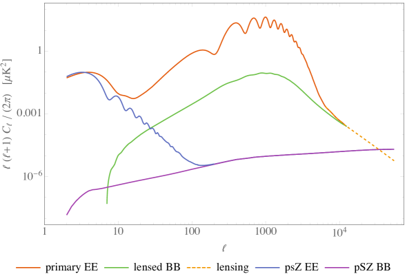
Figure 3 shows the contributions from CEE,pSZ,(0)superscriptsubscript𝐶𝐸𝐸pSZ0C_{\ell}^{EE,\text{pSZ},(0)}, CEE,pSZ,(1)superscriptsubscript𝐶𝐸𝐸pSZ1C_{\ell}^{EE,\text{pSZ},(1)}, and CBB,pSZ,(1)superscriptsubscript𝐶𝐵𝐵pSZ1C_{\ell}^{BB,\text{pSZ},(1)} to the polarized SZ spectrum in comparison to the lensed primary E𝐸E-mode and B𝐵B-mode power spectra. CEE,pSZ,(0)superscriptsubscript𝐶𝐸𝐸pSZ0C_{\ell}^{EE,\text{pSZ},(0)} gives a contribution to the largest scales of the power spectrum, and is in rough agreement with the result from CAMB (which treats reionization more consistently than we do here). On the other hand, CEE,pSZ,(1)superscriptsubscript𝐶𝐸𝐸pSZ1C_{\ell}^{EE,\text{pSZ},(1)} and CBB,pSZ,(1)superscriptsubscript𝐶𝐵𝐵pSZ1C_{\ell}^{BB,\text{pSZ},(1)} are much smaller, and become comparable to the primary CMB only at 3.4×10⁴greater-than-or-equivalent-to3.4superscript104\ell\gtrsim 3.4\times 10^{4}.

Refer to caption
Figure 3: The polarized SZ contribution to the E𝐸E-mode and B𝐵B-mode power spectra in comparison to the primary lensed power spectra (assuming no primordial tensors). CEE,pSZ,(0)superscriptsubscript𝐶𝐸𝐸pSZ0C_{\ell}^{EE,\text{pSZ},(0)} contributes only at low \ell, while CEE,pSZ,(1)superscriptsubscript𝐶𝐸𝐸pSZ1C_{\ell}^{EE,\text{pSZ},(1)} and CBB,pSZ,(1)superscriptsubscript𝐶𝐵𝐵pSZ1C_{\ell}^{BB,\text{pSZ},(1)} dominate the power spectrum around 3.4×10⁴greater-than-or-equivalent-to3.4superscript104\ell\gtrsim 3.4\times 10^{4}. The primary CMB from CAMB is extrapolated to high \ell using the lensing approximation (2.46).

3 Polarized SZ tomography

The pSZ signal is tiny, but it induces a statistically anisotropic cross-correlation with the matter distribution that can be detectable. We call this approach pSZ tomography, in analogy with kSZ tomography [34, 35, 6, 36, 37, 38, 39, 40, 8]. The pSZ signal depends on the local electron density as well as the local CMB quadrupole. In a direction 𝐧^esubscript^𝐧𝑒\hat{\bf n}_{e} and at a comoving distance χesubscript𝜒𝑒\chi_{e} the value of the quadrupole qeff±(𝐧^e,χe)subscriptsuperscript𝑞plus-or-minuseffsubscript^𝐧𝑒subscript𝜒𝑒q^{\pm}_{\rm eff}(\hat{\bf n}_{e},\chi_{e}) modulates the strength of the cross-correlation between the CMB polarization and the electron density field. The CMB quadrupole is a slowly varying, large scale field, while the electron density has a lot of small scale structure. A probe of the quadrupole field is therefore given by the large scale modulation of the local correlation of the high \ell CMB with the matter distribution. This data is the input in our tomography estimator. We now make these ideas precise and estimate the signal to noise.

3.1 Correlation between polarisation and matter due to the pSZ

We first derive the cross correlation between polarisation and matter due to the pSZ effect. We assume the most ideal scenario, in which we have knowledge of the electron density field, which we further assume to trace the dark matter. We also assume a purely Gaussian primordial power spectrum, consistent with the current constraints from Planck [41]. To describe the redshift dependence of the pSZ effect, we introduce a window function W(χe,χ¯e)𝑊subscript𝜒𝑒subscript¯𝜒𝑒W(\chi_{e},\bar{\chi}_{e}) that gives the electron density in a set of redshift bins centered on χe=χ¯esubscript𝜒𝑒subscript¯𝜒𝑒\chi_{e}=\bar{\chi}_{e}

δ(𝐧^e,χ¯e)=𝑑χeW(χe,χ¯e)δ(𝐧^e,χe).𝛿subscript^𝐧𝑒subscript¯𝜒𝑒differential-dsubscript𝜒𝑒𝑊subscript𝜒𝑒subscript¯𝜒𝑒𝛿subscript^𝐧𝑒subscript𝜒𝑒\delta({\bf\hat{n}}_{e},\bar{\chi}_{e})=\int d\chi_{e}W(\chi_{e},\bar{\chi}_{e})\delta({\bf\hat{n}}_{e},\chi_{e}). (3.1)

In this work, we use a top-hat window function normalized to unity, 0χ𝑑χW(χ,χ¯)=1superscriptsubscript0subscript𝜒differential-d𝜒𝑊𝜒¯𝜒1\int_{0}^{\chi_{\infty}}d\chi W(\chi,\bar{\chi})=1, and we consider six redshift bins of equal width, covering the range 0<z<60𝑧60<z<6. The redshift coverage for each bin configuration is shown in table 1.

χ¯esubscript¯𝜒𝑒\bar{\chi}_{e} χesubscript𝜒𝑒\chi_{e} zesubscript𝑧𝑒z_{e}
χ¯e=0.16subscript¯𝜒𝑒0.16\bar{\chi}_{e}=0.16 0.00<χe<0.320.00subscript𝜒𝑒0.320.00<\chi_{e}<0.32 0.00<ze<0.350.00subscript𝑧𝑒0.350.00<z_{e}<0.35
χ¯e=0.48subscript¯𝜒𝑒0.48\bar{\chi}_{e}=0.48 0.32<χe<0.640.32subscript𝜒𝑒0.640.32<\chi_{e}<0.64 0.35<ze<0.780.35subscript𝑧𝑒0.780.35<z_{e}<0.78
χ¯e=0.80subscript¯𝜒𝑒0.80\bar{\chi}_{e}=0.80 0.64<χe<0.960.64subscript𝜒𝑒0.960.64<\chi_{e}<0.96 0.78<ze<1.370.78subscript𝑧𝑒1.370.78<z_{e}<1.37
χ¯e=1.12subscript¯𝜒𝑒1.12\bar{\chi}_{e}=1.12 0.96<χe<1.280.96subscript𝜒𝑒1.280.96<\chi_{e}<1.28 1.37<ze<2.221.37subscript𝑧𝑒2.221.37<z_{e}<2.22
χ¯e=1.44subscript¯𝜒𝑒1.44\bar{\chi}_{e}=1.44 1.28<χe<1.601.28subscript𝜒𝑒1.601.28<\chi_{e}<1.60 2.22<ze<3.592.22subscript𝑧𝑒3.592.22<z_{e}<3.59
χ¯e=1.76subscript¯𝜒𝑒1.76\bar{\chi}_{e}=1.76 1.60<χe<1.921.60subscript𝜒𝑒1.921.60<\chi_{e}<1.92 3.59<ze<6.003.59subscript𝑧𝑒6.003.59<z_{e}<6.00
Table 1: Redshift bins: six equally spaced redshift bins from here (z=0𝑧0z=0) to reionization (z=6𝑧6z=6). The comoving distance is given in units of H01superscriptsubscript𝐻01H_{0}^{-1}.

We first consider the cross-correlation of the Stokes parameters Q±iUplus-or-minus𝑄𝑖𝑈Q\pm iU with the density field δ𝛿\delta which traces the electron distribution, given by

(Q±iU)pSZ(𝐧^e)δ(𝐧^e,χ¯e)=6σT10dχeaen¯e(χe)m=22±2Y2m(𝐧^e)×dχeW(χe,χ¯e)(1+δ(𝐧^e,χe))qeffm(𝐧^e,χe)δ(𝐧^e,χe).delimited-⟨⟩superscriptplus-or-minus𝑄𝑖𝑈pSZsubscript^𝐧𝑒𝛿subscriptsuperscript^𝐧𝑒subscript¯𝜒𝑒6subscript𝜎𝑇10𝑑subscript𝜒𝑒subscript𝑎𝑒subscript¯𝑛𝑒subscript𝜒𝑒superscriptsubscript𝑚22subscriptsubscript𝑌2𝑚plus-or-minus2subscript^𝐧𝑒𝑑subscriptsuperscript𝜒𝑒𝑊subscriptsuperscript𝜒𝑒subscript¯𝜒𝑒delimited-⟨⟩1𝛿subscript^𝐧𝑒subscript𝜒𝑒subscriptsuperscript𝑞𝑚effsubscript^𝐧𝑒subscript𝜒𝑒𝛿superscriptsubscript^𝐧𝑒superscriptsubscript𝜒𝑒\begin{split}\Big{\langle}(Q\pm iU)^{\text{pSZ}}({\bf\hat{n}}_{e})\delta({\bf\hat{n}}^{\prime}_{e},&\bar{\chi}_{e})\Big{\rangle}=-\frac{\sqrt{6}\sigma_{T}}{10}\int d\chi_{e}\,a_{e}\,\bar{n}_{e}(\chi_{e})\sum_{m=-2}^{2}\left.{}_{\pm 2}Y_{2m}\right.({\bf\hat{n}}_{e})\\ &\times\int d\chi^{\prime}_{e}W(\chi^{\prime}_{e},\bar{\chi}_{e})\Big{\langle}(1+\delta({\bf\hat{n}}_{e},\chi_{e}))\ q^{m}_{\rm eff}({\bf\hat{n}}_{e},\chi_{e})\delta({\bf\hat{n}}_{e}^{\prime},\chi_{e}^{\prime})\Big{\rangle}.\end{split} (3.2)

A crucial point for our analysis is that we can isolate large scale inhomogeneities by treating qeffmsubscriptsuperscript𝑞𝑚effq^{m}_{\rm eff} as a slowly varying deterministic field, and treating δ𝛿\delta as a stochastic field with variations on small scales. We’ll now formalize this split between large and small scale contributions to see how it helps achieve our goal of unlocking large scale information. We begin by defining a long and short wavelength decomposition of ΨΨ\Psi,

Ψi(𝐱)=d3k(2π)3(k)Ψi(𝐤)ei𝐤𝐱,Ψi𝒮(𝐱)=d3k(2π)3𝒮(k)Ψi(𝐤)ei𝐤𝐱,formulae-sequencesuperscriptsubscriptΨ𝑖𝐱superscript𝑑3𝑘superscript2𝜋3𝑘subscriptΨ𝑖𝐤superscript𝑒𝑖𝐤𝐱superscriptsubscriptΨ𝑖𝒮𝐱superscript𝑑3𝑘superscript2𝜋3𝒮𝑘subscriptΨ𝑖𝐤superscript𝑒𝑖𝐤𝐱\Psi_{i}^{\mathcal{L}}({\bf x})=\int\frac{d^{3}k}{(2\pi)^{3}}\mathcal{L}(k)\Psi_{i}({\bf k})e^{i{\bf k}\cdot{\bf x}},\ \ \ \ \Psi_{i}^{\mathcal{S}}({\bf x})=\int\frac{d^{3}k}{(2\pi)^{3}}\mathcal{S}(k)\Psi_{i}({\bf k})e^{i{\bf k}\cdot{\bf x}}, (3.3)

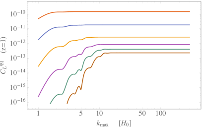
where (k)+𝒮(k)=1𝑘𝒮𝑘1\mathcal{L}(k)+\mathcal{S}(k)=1. For instance, we may choose (k)=ek2/2k2,𝒮(k)=1ek2/2k2formulae-sequence𝑘superscript𝑒superscript𝑘22superscriptsubscript𝑘2𝒮𝑘1superscript𝑒superscript𝑘22superscriptsubscript𝑘2\mathcal{L}(k)=e^{-k^{2}/2k_{*}^{2}},\ \mathcal{S}(k)=1-e^{-k^{2}/2k_{*}^{2}}. We will generally assume k(100Mpc)1similar-tosubscript𝑘superscript100Mpc1k_{*}\sim(100\ \text{Mpc})^{-1}, but the results do not depend on the exact value of ksubscript𝑘k_{*}. The signal described in this section is sensitive only to the deterministic long field formed by scales larger than 100Mpc100Mpc100\ \text{Mpc} (as illustrated later in figure 4) while the noise described in section 3.3 depends mainly on the stochastic short field formed by scales smaller than 100Mpc100Mpc100\ \text{Mpc}.

The decomposition in (3.3) implies a similar long-short split for the quadrupole and density fields, valid in the linear regime

qeffm(𝐧^e,χe)=subscriptsuperscript𝑞𝑚effsubscript^𝐧𝑒subscript𝜒𝑒absent\displaystyle{q^{m}_{\rm eff}}({\bf\hat{n}}_{e},\chi_{e})= qeffm(𝐧^e,χe)+qeffm𝒮(𝐧^e,χe),superscriptsubscriptsuperscript𝑞𝑚effsubscript^𝐧𝑒subscript𝜒𝑒superscriptsubscriptsuperscript𝑞𝑚eff𝒮subscript^𝐧𝑒subscript𝜒𝑒\displaystyle\ {q^{m}_{\rm eff}}^{\mathcal{L}}({\bf\hat{n}}_{e},\chi_{e})+{q^{m}_{\rm eff}}^{\mathcal{S}}({\bf\hat{n}}_{e},\chi_{e}),
δ(𝐧^e,χe)=𝛿subscript^𝐧𝑒subscript𝜒𝑒absent\displaystyle\delta({\bf\hat{n}}_{e},\chi_{e})= δ(𝐧^e,χe)+δ𝒮(𝐧^e,χe).superscript𝛿subscript^𝐧𝑒subscript𝜒𝑒superscript𝛿𝒮subscript^𝐧𝑒subscript𝜒𝑒\displaystyle\ \delta^{\mathcal{L}}({\bf\hat{n}}_{e},\chi_{e})+\delta^{\mathcal{S}}({\bf\hat{n}}_{e},\chi_{e}). (3.4)

Substituting this expansion into the cross-correlation in the second line of (3.2) we obtain

(1+δ)qeffδdelimited-⟨⟩1𝛿subscript𝑞effsuperscript𝛿\displaystyle\langle(1+\delta)\ q_{\text{eff}}\ \delta^{\prime}\rangle =(1+δ+δ𝒮)(qeff+qeff𝒮)(δ+δ𝒮)absentdelimited-⟨⟩1superscript𝛿superscript𝛿𝒮superscriptsubscript𝑞effsuperscriptsubscript𝑞eff𝒮superscriptsuperscript𝛿superscriptsuperscript𝛿𝒮\displaystyle=\ \langle(1+\delta^{\mathcal{L}}+\delta^{\mathcal{S}})\ (q_{\text{eff}}^{\mathcal{L}}+q_{\text{eff}}^{\mathcal{S}})\ ({\delta^{\prime}}^{\mathcal{L}}+{\delta^{\prime}}^{\mathcal{S}})\rangle
=qeffδ+qeffδδ+qeff𝒮δ𝒮+qeffδ𝒮δ𝒮+δqeff𝒮δ𝒮+δqeff𝒮δ𝒮.absentsuperscriptsubscript𝑞effsuperscriptsuperscript𝛿superscriptsubscript𝑞effsuperscript𝛿superscriptsuperscript𝛿delimited-⟨⟩superscriptsubscript𝑞eff𝒮superscriptsuperscript𝛿𝒮superscriptsubscript𝑞effdelimited-⟨⟩superscript𝛿𝒮superscriptsuperscript𝛿𝒮superscript𝛿delimited-⟨⟩superscriptsubscript𝑞eff𝒮superscriptsuperscript𝛿𝒮superscriptsuperscript𝛿delimited-⟨⟩superscriptsubscript𝑞eff𝒮superscript𝛿𝒮\displaystyle\begin{split}&=\ q_{\text{eff}}^{\mathcal{L}}{\delta^{\prime}}^{\mathcal{L}}+q_{\text{eff}}^{\mathcal{L}}\delta^{\mathcal{L}}{\delta^{\prime}}^{\mathcal{L}}+\langle q_{\text{eff}}^{\mathcal{S}}{\delta^{\prime}}^{\mathcal{S}}\rangle\\ &\quad+q_{\text{eff}}^{\mathcal{L}}\langle\delta^{\mathcal{S}}{\delta^{\prime}}^{\mathcal{S}}\rangle+\delta^{\mathcal{L}}\langle q_{\text{eff}}^{\mathcal{S}}{\delta^{\prime}}^{\mathcal{S}}\rangle+{\delta^{\prime}}^{\mathcal{L}}\langle q_{\text{eff}}^{\mathcal{S}}{\delta}^{\mathcal{S}}\rangle.\\ \end{split} (3.5)

The main point of this analysis is that if we want to learn information about large scale inhomogeneities, the ensemble average in eq. (3.2) should only be taken over small scales, leaving large scales as a fixed deterministic field. Above, we have used our assumption of Gaussian fields with zero mean to set to zero any one-point and three-point correlation functions for the short modes. Of the remaining terms, those involving only long modes are a deterministic contribution that shows up only on large angular scales. These terms will be negligible compared to the primary CMB, and are neglected below. The statistically isotropic cross-power between short modes of the density and quadrupole field do not contribute to the signal of interest. Of the three statistically anisotropic terms, only the term qeffδ𝒮δ𝒮superscriptsubscript𝑞effdelimited-⟨⟩superscript𝛿𝒮superscriptsuperscript𝛿𝒮q_{\text{eff}}^{\mathcal{L}}\langle\delta^{\mathcal{S}}{\delta^{\prime}}^{\mathcal{S}}\rangle in (3.5) is significant since the quadrupole field is primarily made up of long-wavelength modes. 444We can estimate the effect of adding bias in as follows. In a purely local bias model to leading order we can assume that δe=b1δ+b2δ2+subscript𝛿𝑒subscript𝑏1𝛿subscript𝑏2superscript𝛿2\delta_{e}=b_{1}\delta+b_{2}\delta^{2}+\ldots. With this assumption, the statistically anisotropic component is given by (1+δe)qeffδdelimited-⟨⟩1subscript𝛿𝑒subscript𝑞effsuperscript𝛿\displaystyle\langle(1+\delta_{e})\ q_{\text{eff}}\ \delta^{\prime}\rangle \displaystyle\subset qeff[b12δ𝒮δ𝒮+b2δ𝒮δ𝒮+b22δ𝒮δ𝒮δ𝒮δ𝒮\displaystyle q_{\text{eff}}^{\mathcal{L}}\left[b_{1}^{2}\langle{\delta}^{\mathcal{S}}{\delta^{\prime}}^{\mathcal{S}}\rangle+b_{2}\langle{\delta^{\prime}}^{\mathcal{S}}{\delta^{\prime}}^{\mathcal{S}}\rangle+b_{2}^{2}\langle{\delta^{\prime}}^{\mathcal{S}}{\delta^{\prime}}^{\mathcal{S}}{\delta}^{\mathcal{S}}{\delta}^{\mathcal{S}}\rangle\right. +\displaystyle+ b1b2δδ𝒮δ𝒮+b1b2δδ𝒮δ𝒮+2b1b2δδ𝒮δ𝒮+𝒪(δ2)]\displaystyle\left.b_{1}b_{2}{\delta^{\prime}}^{\mathcal{L}}\langle{\delta}^{\mathcal{S}}{\delta}^{\mathcal{S}}\rangle+b_{1}b_{2}{\delta}^{\mathcal{L}}\langle{\delta^{\prime}}^{\mathcal{S}}{\delta^{\prime}}^{\mathcal{S}}\rangle+2b_{1}b_{2}{\delta}^{\mathcal{L}}\langle{\delta}^{\mathcal{S}}{\delta^{\prime}}^{\mathcal{S}}\rangle+\mathcal{O}({{\delta}^{\mathcal{L}}}^{2})\right] On linear scales, the density contrast is small (δ1much-less-thansuperscript𝛿1{\delta}^{\mathcal{L}}\ll 1) implying that we can safely neglect the terms in the second line of this equation. What remains is again small scale power modulated by qeffsubscript𝑞effq_{\text{eff}}. Roughly speaking, as long as b12(1+b2/b12)>1superscriptsubscript𝑏121subscript𝑏2superscriptsubscript𝑏121b_{1}^{2}(1+b_{2}/b_{1}^{2})>1 there will be an enhancement in small-scale power over what we have assumed in the main text. Generally speaking, b11subscript𝑏11b_{1}\geq 1, and on non-linear scales one expects b2<0subscript𝑏20b_{2}<0 from the injection of energy due to baryonic feedback effects. At the resolutions assumed in our signal to noise estimates in section 4.2 (max=3000subscriptmax3000\ell_{\rm max}=3000), we do not expect to probe the highly non-linear regime in all but the first redshift bin (for example, scales of 1 Mpc subtend an angle less than π/max𝜋subscriptmax\pi/\ell_{\rm max} for z>0.3𝑧0.3z>0.3). Therefore, we expect that incorporating the linear bias term is sufficient, and we defer a more careful treatment of nonlinear bias (and more realistic tracers!) to future work. This power asymmetry is our desired signal. Using this, we approximate the correlation in eq. (3.2) as

(Q±iU)pSZ(𝐧^e)δ(𝐧^e,χ¯e)=6σT10𝑑χeaen¯e(χe)m=22qeffm(𝐧^e,χe)Y2m±2(𝐧^e)×dχeW(χe,χ¯e)δ(𝐧^e,χe)δ(𝐧^e,χe)+isotropic,delimited-⟨⟩superscriptplus-or-minus𝑄𝑖𝑈pSZsubscript^𝐧𝑒𝛿subscriptsuperscript^𝐧𝑒subscript¯𝜒𝑒6subscript𝜎𝑇10differential-dsubscript𝜒𝑒subscript𝑎𝑒subscript¯𝑛𝑒subscript𝜒𝑒superscriptsubscript𝑚22subscriptsuperscript𝑞𝑚effsubscript^𝐧𝑒subscript𝜒𝑒subscriptsubscript𝑌2𝑚plus-or-minus2subscript^𝐧𝑒𝑑subscriptsuperscript𝜒𝑒𝑊subscriptsuperscript𝜒𝑒subscript¯𝜒𝑒delimited-⟨⟩𝛿subscript^𝐧𝑒subscript𝜒𝑒𝛿superscriptsubscript^𝐧𝑒superscriptsubscript𝜒𝑒isotropic\begin{split}\Big{\langle}(Q\pm iU)^{\text{pSZ}}({\bf\hat{n}}_{e})\delta({\bf\hat{n}}^{\prime}_{e},\bar{\chi}_{e})\Big{\rangle}&=-\frac{\sqrt{6}\sigma_{T}}{10}\int d\chi_{e}a_{e}\bar{n}_{e}(\chi_{e})\sum_{m=-2}^{2}\ q^{m}_{\rm eff}({\bf\hat{n}}_{e},\chi_{e})\left.{}_{\pm 2}Y_{2m}\right.({\bf\hat{n}}_{e})\\ &\times\int d\chi^{\prime}_{e}\ W(\chi^{\prime}_{e},\bar{\chi}_{e})\ \Big{\langle}\delta({\bf\hat{n}}_{e},\chi_{e})\ \delta({\bf\hat{n}}_{e}^{\prime},\chi_{e}^{\prime})\Big{\rangle}+\text{isotropic},\end{split} (3.6)

where we’ve suppressed the 𝒮𝒮\mathcal{S} and \mathcal{L} superscripts, and the density autocorrelation is given in equations (2.38),(2.40). This results motivates an estimator of the remote quadrupole field by cross correlating (Q±iU)plus-or-minus𝑄𝑖𝑈(Q\pm iU) and δ𝛿\delta. However in practice one obtains a better estimator by first splitting the polarisation field into E and B modes, which we will do in the next section.

3.2 Signal calculation

The polarisation (Q±iU)pSZ(𝐧^e)superscriptplus-or-minus𝑄𝑖𝑈pSZsubscript^𝐧𝑒(Q\pm iU)^{\text{pSZ}}({\bf\hat{n}}_{e}) contains both E𝐸E-mode and a B𝐵B-mode components (even from pure scalar perturbations). However, the E𝐸E and B𝐵B mode background, from which we wish to distinguish our signal, have drastically different magnitudes over a large range of angular scales; see Figure 3. To maximize the signal to noise, it is therefore useful to define a set of estimators that are based on the information in the E𝐸E and B𝐵B mode polarization separately. To do so, we define a set of two new spin-2 fields XpSZ±2subscriptsuperscript𝑋pSZplus-or-minus2{}_{\pm 2}X^{\text{pSZ}} based on the scalar X=E,B𝑋𝐸𝐵X=E,B fields:

XpSZ±2(𝐧^e)=mXmpSZYLM±2(𝐧^e)subscriptsuperscript𝑋pSZplus-or-minus2subscript^𝐧𝑒subscript𝑚subscriptsuperscript𝑋pSZ𝑚subscriptsuperscriptsubscript𝑌𝐿𝑀plus-or-minus2subscript^𝐧𝑒{}_{\pm 2}X^{\text{pSZ}}({\bf\hat{n}}_{e})=\sum_{\ell m}X^{\text{pSZ}}_{\ell m}\ {}_{\pm 2}Y_{LM}^{*}({\bf\hat{n}}_{e}) (3.7)

In each redshift bin we calculate the expected correlation

aLMX±2d2n^eYLM±2(𝐧^e)XpSZ±2(𝐧^e)δ(𝐧^e,χ¯e).subscriptsubscriptsuperscript𝑎𝑋𝐿𝑀plus-or-minus2superscript𝑑2subscript^𝑛𝑒subscriptsuperscriptsubscript𝑌𝐿𝑀plus-or-minus2subscript^𝐧𝑒delimited-⟨⟩subscriptsuperscript𝑋pSZplus-or-minus2subscript^𝐧𝑒𝛿subscript^𝐧𝑒subscript¯𝜒𝑒{}_{\pm 2}a^{X}_{LM}\equiv\int d^{2}\hat{n}_{e}\ {}_{\pm 2}Y_{LM}^{*}({\bf\hat{n}}_{e})\Big{\langle}{}_{\pm 2}X^{\text{pSZ}}({\bf\hat{n}}_{e})\delta({\bf\hat{n}}_{e},\bar{\chi}_{e})\Big{\rangle}. (3.8)

Importantly, the above quantity allows us to isolate the statistically anisotropic term in eq. (3.6), which makes it possible to measure the effective quadrupole. Since the effective quadrupole is related to the primordial potential as in eq. (2.14), this provides a way to measure large scale inhomogeneities.

For the correlator of XpSZ±2subscriptsuperscript𝑋pSZplus-or-minus2{}_{\pm 2}X^{\text{pSZ}} with matter, assuming only scalar perturbations we obtain, using Eq. (2.3) and (2.3)

XpSZ±2(𝐧^e)δ(𝐧^e,χ¯e)=delimited-⟨⟩subscriptsuperscript𝑋pSZplus-or-minus2subscript^𝐧𝑒𝛿subscript^𝐧𝑒subscript¯𝜒𝑒absent\displaystyle\Big{\langle}{}_{\pm 2}X^{\text{pSZ}}({\bf\hat{n}}_{e})\delta({\bf\hat{n}}_{e},\bar{\chi}_{e})\Big{\rangle}= 6σT10𝑑χeaen¯e(χe)1,m12,m2,mY1m1±2(𝐧^e)Y2m2(𝐧^e)6subscript𝜎𝑇10differential-dsubscript𝜒𝑒subscript𝑎𝑒subscript¯𝑛𝑒subscript𝜒𝑒subscriptsubscript1subscript𝑚1subscriptsubscript2subscript𝑚2subscript𝑚subscriptsubscript𝑌subscript1subscript𝑚1plus-or-minus2subscript^𝐧𝑒subscript𝑌subscript2subscript𝑚2subscript^𝐧𝑒\displaystyle\frac{\sqrt{6}\ \sigma_{T}}{10}\int d\chi_{e}\ a_{e}\bar{n}_{e}(\chi_{e})\sum_{\ell_{1},m_{1}}\sum_{\ell_{2},m_{2}}\sum_{\ell,m}{}_{\pm 2}Y_{\ell_{1}m_{1}}({\bf\hat{n}}_{e})Y_{\ell_{2}m_{2}}({\bf\hat{n}}_{e})
12i(1±(1)1+2+)(21+1)(22+1)(2+1)4π(1)m112𝑖plus-or-minus1superscript1subscript1subscript22subscript112subscript21214𝜋superscript1subscript𝑚1\displaystyle\frac{1}{2i}\left(1\pm(-1)^{\ell_{1}+\ell_{2}+\ell}\right)\sqrt{\frac{(2\ell_{1}+1)(2\ell_{2}+1)(2\ell+1)}{4\pi}}(-1)^{m_{1}}
×(12m1m2m)(12202)C2δδ(χe)amq(χe).absentsubscript1subscript2subscript𝑚1subscript𝑚2𝑚subscript1subscript2202superscriptsubscript𝐶subscript2𝛿𝛿subscript𝜒𝑒superscriptsubscript𝑎𝑚𝑞subscript𝜒𝑒\displaystyle\times\left(\begin{array}[]{ccc}\ell_{1}&\ell_{2}&\ell\\ -m_{1}&-m_{2}&m\end{array}\right)\left(\begin{array}[]{ccc}\ell_{1}&\ell_{2}&\ell\\ -2&0&2\end{array}\right)C_{\ell_{2}}^{\delta\delta}(\chi_{e})a_{\ell m}^{q}(\chi_{e}). (3.13)

where in the (1±(1)1+2+)plus-or-minus1superscript1subscript1subscript2(1\pm(-1)^{\ell_{1}+\ell_{2}+\ell}) factor the positive sign is for X=E𝑋𝐸X=E and the negative sign for X=B𝑋𝐵X=B. Plugging the correlator in Eq. (3.8) we obtain

aLMX±2(χ¯e)=subscriptsubscriptsuperscript𝑎𝑋𝐿𝑀plus-or-minus2subscript¯𝜒𝑒absent\displaystyle{}_{\pm 2}a^{X}_{LM}(\bar{\chi}_{e})= 6σT10𝑑χeaen¯e(χe)𝑑χeW(χe,χ¯e)6subscript𝜎𝑇10differential-dsubscript𝜒𝑒subscript𝑎𝑒subscript¯𝑛𝑒subscript𝜒𝑒differential-dsubscriptsuperscript𝜒𝑒𝑊subscriptsuperscript𝜒𝑒subscript¯𝜒𝑒\displaystyle\frac{\sqrt{6}\ \sigma_{T}}{10}\int d\chi_{e}\ a_{e}\bar{n}_{e}(\chi_{e})\int d\chi^{\prime}_{e}\ W(\chi^{\prime}_{e},\bar{\chi}_{e})
1212i(1±(1)1+2+L)(21+1)(22+1)4πsubscriptsubscript1subscript212𝑖plus-or-minus1superscript1subscript1subscript2𝐿2subscript112subscript214𝜋\displaystyle\sum_{\ell_{1}\ell_{2}}\frac{1}{2i}\left(1\pm(-1)^{\ell_{1}+\ell_{2}+L}\right)\frac{(2\ell_{1}+1)(2\ell_{2}+1)}{4\pi}
×(12L202)(12L±202)C2δδ(χe,χe)aLMq(χe)absentsubscript1subscript2𝐿202subscript1subscript2𝐿plus-or-minus20minus-or-plus2superscriptsubscript𝐶subscript2𝛿𝛿subscript𝜒𝑒subscriptsuperscript𝜒𝑒superscriptsubscript𝑎𝐿𝑀𝑞subscript𝜒𝑒\displaystyle\times\left(\begin{array}[]{ccc}\ell_{1}&\ell_{2}&L\\ -2&0&2\end{array}\right)\left(\begin{array}[]{ccc}\ell_{1}&\ell_{2}&L\\ \pm 2&0&\mp 2\end{array}\right)C_{\ell_{2}}^{\delta\delta}(\chi_{e},\chi^{\prime}_{e})a_{LM}^{q}(\chi_{e}) (3.18)

Finally, we define a set of scalar multipole moments

eLMsubscript𝑒𝐿𝑀\displaystyle e_{LM} =\displaystyle= 12(aLME+2+aLME2),12subscriptsubscriptsuperscript𝑎𝐸𝐿𝑀2subscriptsubscriptsuperscript𝑎𝐸𝐿𝑀2\displaystyle\frac{1}{2}\left({}_{+2}a^{E}_{LM}+{}_{-2}a^{E}_{LM}\right), (3.19)
bLMsubscript𝑏𝐿𝑀\displaystyle b_{LM} =\displaystyle= 12i(aLMB+2aLMB2),12𝑖subscriptsubscriptsuperscript𝑎𝐵𝐿𝑀2subscriptsubscriptsuperscript𝑎𝐵𝐿𝑀2\displaystyle\frac{1}{2i}\left({}_{+2}a^{B}_{LM}-{}_{-2}a^{B}_{LM}\right), (3.20)

Inserting CLδδ(χe,χe)superscriptsubscript𝐶superscript𝐿𝛿𝛿subscript𝜒𝑒subscriptsuperscript𝜒𝑒C_{L^{\prime}}^{\delta\delta}(\chi_{e},\chi^{\prime}_{e}) from Eq. 2.40 and applying the Limber approximation we obtain

bLM(χ¯e)=subscript𝑏𝐿𝑀subscript¯𝜒𝑒absent\displaystyle b_{LM}(\bar{\chi}_{e})= 6σT101214(1(1)1+2+L)2(21+1)(22+1)4π(12L202)26subscript𝜎𝑇10subscriptsubscript1subscript214superscript1superscript1subscript1subscript2𝐿22subscript112subscript214𝜋superscriptsubscript1subscript2𝐿2022\displaystyle\frac{\sqrt{6}\ \sigma_{T}}{10}\sum_{\ell_{1}\ell_{2}}\frac{1}{4}\left(1-(-1)^{\ell_{1}+\ell_{2}+L}\right)^{2}\frac{(2\ell_{1}+1)(2\ell_{2}+1)}{4\pi}\left(\begin{array}[]{ccc}\ell_{1}&\ell_{2}&L\\ -2&0&2\end{array}\right)^{2} (3.23)
dχeχe2aen¯e(χe)W(χe,χ¯e)aLMq(χe)Pδ(2+1/2χe,χe)𝑑subscript𝜒𝑒superscriptsubscript𝜒𝑒2subscript𝑎𝑒subscript¯𝑛𝑒subscript𝜒𝑒𝑊subscript𝜒𝑒subscript¯𝜒𝑒superscriptsubscript𝑎𝐿𝑀𝑞subscript𝜒𝑒subscript𝑃𝛿subscript212subscript𝜒𝑒subscript𝜒𝑒\displaystyle\int\frac{d\chi_{e}}{\chi_{e}^{2}}\ a_{e}\bar{n}_{e}(\chi_{e})W(\chi_{e},\bar{\chi}_{e})a_{LM}^{q}(\chi_{e})P_{\delta}\left(\frac{\ell_{2}+1/2}{\chi_{e}},\chi_{e}\right) (3.24)

and

eLM(χ¯e)=subscript𝑒𝐿𝑀subscript¯𝜒𝑒absent\displaystyle e_{LM}(\bar{\chi}_{e})= 6σT101214(1+(1)1+2+L)2(21+1)(22+1)4π(12L202)26subscript𝜎𝑇10subscriptsubscript1subscript214superscript1superscript1subscript1subscript2𝐿22subscript112subscript214𝜋superscriptsubscript1subscript2𝐿2022\displaystyle\frac{\sqrt{6}\ \sigma_{T}}{10}\sum_{\ell_{1}\ell_{2}}\frac{1}{4}\left(1+(-1)^{\ell_{1}+\ell_{2}+L}\right)^{2}\frac{(2\ell_{1}+1)(2\ell_{2}+1)}{4\pi}\left(\begin{array}[]{ccc}\ell_{1}&\ell_{2}&L\\ -2&0&2\end{array}\right)^{2} (3.28)
dχeχe2aen¯e(χe)W(χe,χ¯e)aLMq(χe)Pδ(2+1/2χe,χe)𝑑subscript𝜒𝑒superscriptsubscript𝜒𝑒2subscript𝑎𝑒subscript¯𝑛𝑒subscript𝜒𝑒𝑊subscript𝜒𝑒subscript¯𝜒𝑒superscriptsubscript𝑎𝐿𝑀𝑞subscript𝜒𝑒subscript𝑃𝛿subscript212subscript𝜒𝑒subscript𝜒𝑒\displaystyle\int\frac{d\chi_{e}}{\chi_{e}^{2}}\ a_{e}\bar{n}_{e}(\chi_{e})W(\chi_{e},\bar{\chi}_{e})a_{LM}^{q}(\chi_{e})P_{\delta}\left(\frac{\ell_{2}+1/2}{\chi_{e}},\chi_{e}\right) (3.29)

We thus find that the large-scale quadrupole induces E-mode and B-mode modulations of the correlation of CMB and matter, both of which are proportional to the multipoles aLMqsuperscriptsubscript𝑎𝐿𝑀𝑞a_{LM}^{q}. We can thus use this correlation as a probe of aLMqsuperscriptsubscript𝑎𝐿𝑀𝑞a_{LM}^{q}.

3.3 Variance calculation

In this section we calculate the Gaussian variance of the estimator e^LMsubscript^𝑒𝐿𝑀\hat{e}_{LM} and e^LMsubscript^𝑒𝐿𝑀\hat{e}_{LM} in the absence of the pSZ signal induced by the remote quadrupole field. Our estimator (indicated notationally by the overhead) is defined as

e^LMsubscript^𝑒𝐿𝑀\displaystyle\hat{e}_{LM} =\displaystyle= 12(a^LME+2+a^LME2),12subscriptsubscriptsuperscript^𝑎𝐸𝐿𝑀2subscriptsubscriptsuperscript^𝑎𝐸𝐿𝑀2\displaystyle\frac{1}{2}\left({}_{+2}\hat{a}^{E}_{LM}+{}_{-2}\hat{a}^{E}_{LM}\right), (3.30)
b^LMsubscript^𝑏𝐿𝑀\displaystyle\hat{b}_{LM} =\displaystyle= 12i(a^LMB+2a^LMB2),12𝑖subscriptsubscriptsuperscript^𝑎𝐵𝐿𝑀2subscriptsubscriptsuperscript^𝑎𝐵𝐿𝑀2\displaystyle\frac{1}{2i}\left({}_{+2}\hat{a}^{B}_{LM}-{}_{-2}\hat{a}^{B}_{LM}\right), (3.31)

with

a^LMX±2d2n^eYLM±2(𝐧^e)XpSZ±2(𝐧^e)δ(𝐧^e,χ¯e).subscriptsubscriptsuperscript^𝑎𝑋𝐿𝑀plus-or-minus2superscript𝑑2subscript^𝑛𝑒subscriptsuperscriptsubscript𝑌𝐿𝑀plus-or-minus2subscript^𝐧𝑒subscriptsuperscript𝑋pSZplus-or-minus2subscript^𝐧𝑒𝛿subscript^𝐧𝑒subscript¯𝜒𝑒{}_{\pm 2}\hat{a}^{X}_{LM}\equiv\int d^{2}\hat{n}_{e}\ {}_{\pm 2}Y_{LM}^{*}({\bf\hat{n}}_{e}){}_{\pm 2}X^{\text{pSZ}}({\bf\hat{n}}_{e})\delta({\bf\hat{n}}_{e},\bar{\chi}_{e}). (3.32)

To make the separation between large scales and small scales concrete, we filter both the CMB map X𝑋X and the matter map δ𝛿\delta with a high pass filter >minsubscriptmin\ell>\ell_{\rm min}.

We now calculate the variance of this estimator, which corresponds to an accidental power asymmetry in the cross-correlation in the absence of the remote quadrupole field. Starting with the bLMsubscript𝑏𝐿𝑀b_{LM} , we compute:

b^LM(χ¯e)b^LM(χ¯e)=14(a^LMB+2a^LMB2)(a^LMB+2a^LMB2)delimited-⟨⟩subscriptsuperscript^𝑏𝐿𝑀subscript¯𝜒𝑒subscript^𝑏𝐿𝑀subscript¯𝜒𝑒14delimited-⟨⟩subscriptsubscriptsuperscript^𝑎𝐵𝐿𝑀2subscriptsubscriptsuperscript^𝑎𝐵𝐿𝑀2subscriptsubscriptsuperscript^𝑎𝐵𝐿𝑀2subscriptsubscriptsuperscript^𝑎𝐵𝐿𝑀2\begin{split}\Big{\langle}\hat{b}^{*}_{LM}(\bar{\chi}_{e})\hat{b}_{LM}(\bar{\chi}_{e})\Big{\rangle}&=\frac{1}{4}\Big{\langle}({}_{+2}\hat{a}^{B*}_{LM}-{}_{-2}\hat{a}^{B*}_{LM})({}_{+2}\hat{a}^{B}_{LM}-{}_{-2}\hat{a}^{B}_{LM})\Big{\rangle}\end{split} (3.33)

where χ¯esubscript¯𝜒𝑒\bar{\chi}_{e} represents the center of the redshift bin. This variance quantifies the chance power asymmetry that is present in the statistically isotropic contribution to E,B𝐸𝐵E,B, which is sensitive mainly to small scales. For example the first term gives

a^LMB+2a^LMB+2=d2𝐧^ed2𝐧^eYLM+2(𝐧^e)YLM+2(𝐧^e)B+2(𝐧^e)δ(𝐧^e,χ¯e)B+2(𝐧^e)δ(𝐧^e,χ¯e)d2𝐧^ed2𝐧^eYLM+2(𝐧^e)YLM+2(𝐧^e)B+2(𝐧^e)B+2(𝐧^e)δ(𝐧^e,χ¯e)δ(𝐧^e,χ¯e),delimited-⟨⟩subscriptsubscriptsuperscript^𝑎𝐵𝐿𝑀2subscriptsubscriptsuperscript^𝑎𝐵𝐿𝑀2superscript𝑑2subscript^𝐧𝑒superscript𝑑2subscriptsuperscript^𝐧𝑒subscriptsubscript𝑌𝐿𝑀2subscript^𝐧𝑒subscriptsubscriptsuperscript𝑌𝐿𝑀2subscriptsuperscript^𝐧𝑒delimited-⟨⟩subscript𝐵2subscript^𝐧𝑒𝛿subscript^𝐧𝑒subscript¯𝜒𝑒subscript𝐵2subscriptsuperscript^𝐧𝑒𝛿subscriptsuperscript^𝐧𝑒subscript¯𝜒𝑒similar-to-or-equalssuperscript𝑑2subscript^𝐧𝑒superscript𝑑2subscriptsuperscript^𝐧𝑒subscriptsubscript𝑌𝐿𝑀2subscript^𝐧𝑒subscriptsubscriptsuperscript𝑌𝐿𝑀2subscriptsuperscript^𝐧𝑒delimited-⟨⟩subscript𝐵2subscript^𝐧𝑒subscript𝐵2subscriptsuperscript^𝐧𝑒delimited-⟨⟩𝛿subscript^𝐧𝑒subscript¯𝜒𝑒𝛿subscriptsuperscript^𝐧𝑒subscript¯𝜒𝑒\begin{split}\Big{\langle}{}_{+2}\hat{a}^{B*}_{LM}{}_{+2}\hat{a}^{B}_{LM}\Big{\rangle}&=\int d^{2}{\bf\hat{n}}_{e}d^{2}{\bf\hat{n}}^{\prime}_{e}\ {}_{+2}Y_{LM}({\bf\hat{n}}_{e})\ {}_{+2}Y^{*}_{LM}({\bf\hat{n}}^{\prime}_{e})\Big{\langle}{}_{+2}B({\bf\hat{n}}_{e})\ \delta({\bf\hat{n}}_{e},\bar{\chi}_{e})\ {}_{+2}B({\bf\hat{n}}^{\prime}_{e})\ \delta({\bf\hat{n}}^{\prime}_{e},\bar{\chi}_{e})\Big{\rangle}\\ &\simeq\int d^{2}{\bf\hat{n}}_{e}d^{2}{\bf\hat{n}}^{\prime}_{e}\ {}_{+2}Y_{LM}({\bf\hat{n}}_{e})\ {}_{+2}Y^{*}_{LM}({\bf\hat{n}}^{\prime}_{e})\Big{\langle}{}_{+2}B({\bf\hat{n}}_{e})\ {}_{+2}B({\bf\hat{n}}^{\prime}_{e})\Big{\rangle}\Big{\langle}\delta({\bf\hat{n}}_{e},\bar{\chi}_{e})\ \delta({\bf\hat{n}}^{\prime}_{e},\bar{\chi}_{e})\Big{\rangle},\end{split} (3.34)

where in the second line we have dropped the two largely subdominant cross correlation terms.

The binned matter density power spectrum is given by

δ(𝐧^e,χ¯e)δ(𝐧^e,χ¯e)=,mCδδYm(𝐧^e)Ym(𝐧^e),delimited-⟨⟩𝛿subscript^𝐧𝑒subscript¯𝜒𝑒𝛿subscriptsuperscript^𝐧𝑒subscript¯𝜒𝑒subscript𝑚superscriptsubscript𝐶𝛿𝛿subscriptsuperscript𝑌𝑚subscript^𝐧𝑒subscript𝑌𝑚subscriptsuperscript^𝐧𝑒\Big{\langle}\delta({\bf\hat{n}}_{e},\bar{\chi}_{e})\ \delta({\bf\hat{n}}^{\prime}_{e},\bar{\chi}_{e})\Big{\rangle}=\sum_{\ell,m}C_{\ell}^{\delta\delta}\ Y^{*}_{\ell m}({\bf\hat{n}}_{e})\ Y_{\ell m}({\bf\hat{n}}^{\prime}_{e}), (3.35)

with

Cδδ(χ¯e)=superscriptsubscript𝐶𝛿𝛿subscript¯𝜒𝑒absent\displaystyle C_{\ell}^{\delta\delta}(\bar{\chi}_{e})= 𝑑χeW(χe,χ¯e)𝑑χeW(χe,χ¯e)Cδδ(χe,χe)differential-dsubscript𝜒𝑒𝑊subscript𝜒𝑒subscript¯𝜒𝑒differential-dsubscriptsuperscript𝜒𝑒𝑊subscriptsuperscript𝜒𝑒subscript¯𝜒𝑒superscriptsubscript𝐶𝛿𝛿subscript𝜒𝑒subscriptsuperscript𝜒𝑒\displaystyle\int d\chi_{e}\ W(\chi_{e},\bar{\chi}_{e})\int d\chi^{\prime}_{e}\ W(\chi^{\prime}_{e},\bar{\chi}_{e})\ C_{\ell}^{\delta\delta}(\chi_{e},\chi^{\prime}_{e})
=\displaystyle= 𝑑k2k2π𝑑χePδ(k,χe)W(χe,χ¯e)j(kχe)𝑑χePδ(k,χe)W(χe,χ¯e)j(kχe)differential-d𝑘2superscript𝑘2𝜋differential-dsubscript𝜒𝑒subscript𝑃𝛿𝑘subscript𝜒𝑒𝑊subscript𝜒𝑒subscript¯𝜒𝑒subscript𝑗𝑘subscript𝜒𝑒differential-dsubscriptsuperscript𝜒𝑒subscript𝑃𝛿𝑘subscriptsuperscript𝜒𝑒𝑊subscriptsuperscript𝜒𝑒subscript¯𝜒𝑒subscript𝑗𝑘subscriptsuperscript𝜒𝑒\displaystyle\int dk\frac{2k^{2}}{\pi}\int d\chi_{e}\sqrt{P_{\delta}(k,\chi_{e})}W(\chi_{e},\bar{\chi}_{e})j_{\ell}(k\chi_{e})\int d\chi^{\prime}_{e}\sqrt{P_{\delta}(k,\chi^{\prime}_{e})}W(\chi^{\prime}_{e},\bar{\chi}_{e})j_{\ell}(k\chi^{\prime}_{e})
similar-to-or-equals\displaystyle\simeq dk+1/2W2(+1/2k,χ¯e)Pδ(k,+1/2k),𝑑𝑘12superscript𝑊212𝑘subscript¯𝜒𝑒subscript𝑃𝛿𝑘12𝑘\displaystyle\int\frac{dk}{\ell+1/2}W^{2}\left(\frac{\ell+1/2}{k},\bar{\chi}_{e}\right)P_{\delta}\left(k,\frac{\ell+1/2}{k}\right), (3.36)

where we used the expression for Cδδ(χe,χe)superscriptsubscript𝐶𝛿𝛿subscript𝜒𝑒subscriptsuperscript𝜒𝑒C_{\ell}^{\delta\delta}(\chi_{e},\chi^{\prime}_{e}) from (2.40), and the Limber approximation in the last line.

The CMB power spectra CXXsuperscriptsubscript𝐶𝑋𝑋C_{\ell}^{XX} are given by

X±2(𝐧^e)X±2(𝐧^e)=,mCXXYm±2(𝐧^e)Ym±2(𝐧^e),delimited-⟨⟩subscript𝑋plus-or-minus2subscript^𝐧𝑒subscript𝑋plus-or-minus2subscriptsuperscript^𝐧𝑒subscript𝑚superscriptsubscript𝐶𝑋𝑋subscriptsubscriptsuperscript𝑌𝑚plus-or-minus2subscript^𝐧𝑒subscriptsubscript𝑌𝑚plus-or-minus2subscriptsuperscript^𝐧𝑒\begin{split}\Big{\langle}{}_{\pm 2}X({\bf\hat{n}}_{e}){}_{\pm 2}X({\bf\hat{n}}^{\prime}_{e})\Big{\rangle}=&\sum_{\ell,m}C_{\ell}^{XX}\ {}_{\pm 2}Y^{*}_{\ell m}({\bf\hat{n}}_{e})\ {}_{\pm 2}Y_{\ell m}({\bf\hat{n}}^{\prime}_{e}),\end{split} (3.37)

The contributions to the E𝐸E-mode and B𝐵B-mode power spectra at the high \ell of our interest are

CEEsuperscriptsubscript𝐶𝐸𝐸\displaystyle C_{\ell}^{EE} =\displaystyle= CEE,lensed+CEE,pSZ,superscriptsubscript𝐶𝐸𝐸lensedsuperscriptsubscript𝐶𝐸𝐸pSZ\displaystyle C_{\ell}^{EE,\text{lensed}}+C_{\ell}^{EE,\text{pSZ}}, (3.38)
CBBsuperscriptsubscript𝐶𝐵𝐵\displaystyle C_{\ell}^{BB} =\displaystyle= CBB,lensed+CBB,pSZ,superscriptsubscript𝐶𝐵𝐵lensedsuperscriptsubscript𝐶𝐵𝐵pSZ\displaystyle C_{\ell}^{BB,\text{lensed}}+C_{\ell}^{BB,\text{pSZ}}, (3.39)

for which we can recall the expressions for CEE,pSZsuperscriptsubscript𝐶𝐸𝐸pSZC_{\ell}^{EE,\text{pSZ}}, CEE,lensedsuperscriptsubscript𝐶𝐸𝐸lensedC_{\ell}^{EE,\text{lensed}}, CBB,lensedsuperscriptsubscript𝐶𝐵𝐵lensedC_{\ell}^{BB,\text{lensed}}, and CBB,pSZsuperscriptsubscript𝐶𝐵𝐵pSZC_{\ell}^{BB,\text{pSZ}} from equations (C.15), (2.45), and (2.46). The various terms are plotted in Figure 3.

Plugging these expressions into the first term of the variance we obtain

a^LMB+2a^LMB+2=,,m,mCBBCδδ(χ¯e)(2L+1)(2+1)(2+1)4π×(LMmm)2(L+220)2delimited-⟨⟩subscriptsubscriptsuperscript^𝑎𝐵𝐿𝑀2subscriptsubscriptsuperscript^𝑎𝐵𝐿𝑀2subscriptsuperscript𝑚superscript𝑚superscriptsubscript𝐶𝐵𝐵superscriptsubscript𝐶superscript𝛿𝛿subscript¯𝜒𝑒2𝐿1212superscript14𝜋superscript𝐿superscript𝑀𝑚superscript𝑚2superscript𝐿superscript2202\begin{split}\Big{\langle}{}_{+2}\hat{a}^{B*}_{LM}{}_{+2}\hat{a}^{B}_{LM}\Big{\rangle}&=\sum_{\ell,\ell^{\prime},m,m^{\prime}}C_{\ell}^{BB}\ C_{\ell^{\prime}}^{\delta\delta}(\bar{\chi}_{e})\frac{(2L+1)(2\ell+1)(2\ell^{\prime}+1)}{4\pi}\\ &\times\left(\begin{array}[]{ccc}L&\ell&\ell^{\prime}\\ M&-m&-m^{\prime}\end{array}\right)^{2}\left(\begin{array}[]{ccc}L&\ell&\ell^{\prime}\\ +2&-2&0\end{array}\right)^{2}\end{split} (3.40)

Including all permuations and using the orthogonality relation of the 3j-symbols the final result for the B-mode variance is

b^L(χe¯)2=12,=minmaxCBBCδδ(χ¯e)(2+1)(2+1)4π(L+220)2delimited-⟨⟩subscript^𝑏𝐿superscript¯subscript𝜒𝑒212superscriptsubscriptsuperscriptsubscriptminsubscriptmaxsuperscriptsubscript𝐶𝐵𝐵superscriptsubscript𝐶superscript𝛿𝛿subscript¯𝜒𝑒212superscript14𝜋superscript𝐿superscript2202\begin{split}\Big{\langle}\hat{b}_{L}(\bar{\chi_{e}})^{2}\Big{\rangle}=\frac{1}{2}\sum_{\ell,\ell^{\prime}=\ell_{\text{min}}}^{\ell_{\text{max}}}C_{\ell}^{BB}\ C_{\ell^{\prime}}^{\delta\delta}(\bar{\chi}_{e})\frac{(2\ell+1)(2\ell^{\prime}+1)}{4\pi}\left(\begin{array}[]{ccc}L&\ell&\ell^{\prime}\\ +2&-2&0\end{array}\right)^{2}\end{split} (3.41)

and for the E-modes

e^L(χe¯)2=12,=minmaxCEECδδ(χ¯e)(2+1)(2+1)4π(L+220)2delimited-⟨⟩subscript^𝑒𝐿superscript¯subscript𝜒𝑒212superscriptsubscriptsuperscriptsubscriptminsubscriptmaxsuperscriptsubscript𝐶𝐸𝐸superscriptsubscript𝐶superscript𝛿𝛿subscript¯𝜒𝑒212superscript14𝜋superscript𝐿superscript2202\begin{split}\Big{\langle}\hat{e}_{L}(\bar{\chi_{e}})^{2}\Big{\rangle}=\frac{1}{2}\sum_{\ell,\ell^{\prime}=\ell_{\text{min}}}^{\ell_{\text{max}}}C_{\ell}^{EE}\ C_{\ell^{\prime}}^{\delta\delta}(\bar{\chi}_{e})\frac{(2\ell+1)(2\ell^{\prime}+1)}{4\pi}\left(\begin{array}[]{ccc}L&\ell&\ell^{\prime}\\ +2&-2&0\end{array}\right)^{2}\end{split} (3.42)

Note that the 3-j𝑗j symbols are only nonzero for |L|+L𝐿superscript𝐿|\ell-L|\leq\ell^{\prime}\leq\ell+L. Just as for the signal, the lower and upper bounds on the sum have been introduced to represent the experimental filtering and resolution scales.

4 Experimental forecast

In this section, we explore the sensitivity and resolution requirements to detect the pSZ signal, and compare with what is attainable in future experiments. Our strategy will be to assume a cosmic-variance limited measurement out to a fiducial choice for max=3000subscriptmax3000\ell_{\rm max}=3000, determine the required resolution and sensitivity of a CMB polarization experiment and galaxy survey to achieve this, and then compute the signal-to-noise ratio (SNR) in the 6-redshift bin configuration.

4.1 Experimental requirements

Assuming that the instrumental noise is a uniform Gaussian random field, the total observed CMB E𝐸E-mode and B𝐵B-mode power spectra can be written as a sum of three different contributions:

CEE=subscriptsuperscript𝐶𝐸𝐸absent\displaystyle C^{EE}_{\ell}= (CEE,lensed+CEE,pSZ+NEE)exp[(+1)θFWHM28ln2],superscriptsubscript𝐶𝐸𝐸lensedsuperscriptsubscript𝐶𝐸𝐸pSZsuperscript𝑁𝐸𝐸1subscriptsuperscript𝜃2FWHM82\displaystyle\left(C_{\ell}^{EE,\text{lensed}}+C_{\ell}^{EE,\text{pSZ}}+N^{EE}\right)\exp\left[\frac{\ell(\ell+1)\theta^{2}_{\text{FWHM}}}{8\ln 2}\right], (4.1)
CBB=subscriptsuperscript𝐶𝐵𝐵absent\displaystyle C^{BB}_{\ell}= (CBB,lensed+CBB,pSZ+NBB)exp[(+1)θFWHM28ln2],superscriptsubscript𝐶𝐵𝐵lensedsuperscriptsubscript𝐶𝐵𝐵pSZsuperscript𝑁𝐵𝐵1subscriptsuperscript𝜃2FWHM82\displaystyle\left(C_{\ell}^{BB,\text{lensed}}+C_{\ell}^{BB,\text{pSZ}}+N^{BB}\right)\exp\left[\frac{\ell(\ell+1)\theta^{2}_{\text{FWHM}}}{8\ln 2}\right], (4.2)

where θFWHMsubscript𝜃FWHM\theta_{\text{FWHM}} is the full width at half maximum (expressed in radians), and CEE,lensedsuperscriptsubscript𝐶𝐸𝐸lensedC_{\ell}^{EE,\text{lensed}}, CEE,pSZsuperscriptsubscript𝐶𝐸𝐸pSZC_{\ell}^{EE,\text{pSZ}} and NEEsuperscript𝑁𝐸𝐸N^{EE} denote the lensed primary E𝐸E-mode power spectrum, the high-\ell pSZ power, and the (gaussian, white) instrumental noise respectively; the corresponding quantities are also defined for the B𝐵B-modes.

For a given maxsubscriptmax\ell_{\text{max}}, the corresponding angular resolution (in radians) required is

θFWHM=8ln2max(max+1).subscript𝜃FWHM82subscriptmaxsubscriptmax1\theta_{\text{FWHM}}=\sqrt{\frac{8\ln 2}{\ell_{\text{max}}(\ell_{\text{max}}+1)}}. (4.3)

For maxsubscriptmax\ell_{\text{max}} this translates to θFWHM=2.7arcminsubscript𝜃FWHM2.7arcmin\theta_{\text{FWHM}}=2.7\ {\rm arcmin}. The required sensitivity can then be set by matching the power of the noise NXXsuperscript𝑁𝑋𝑋N^{XX} to the power of the other contributions to the X=E,B𝑋𝐸𝐵X=E,B modes at maxsubscriptmax\ell_{\text{max}}:

NXX=CmaxXX,lensed+CmaxXX,pSZ.superscript𝑁𝑋𝑋superscriptsubscript𝐶subscriptmax𝑋𝑋lensedsuperscriptsubscript𝐶subscriptmax𝑋𝑋pSZ\displaystyle N^{XX}=C_{\ell_{\text{max}}}^{XX,\text{lensed}}+C_{\ell_{\text{max}}}^{XX,\text{pSZ}}. (4.4)

For max=3000subscriptmax3000\ell_{\text{max}}=3000, and using the E𝐸E and B𝐵B mode power spectra shown in Figure 3, this translates to NEE3μKarcminsimilar-to-or-equalssuperscript𝑁𝐸𝐸3𝜇KarcminN^{EE}\simeq 3\ \mu{\rm K}\ {\rm arcmin} and NBB0.3μKarcminsimilar-to-or-equalssuperscript𝑁𝐵𝐵0.3𝜇KarcminN^{BB}\simeq 0.3\ \mu{\rm K}\ {\rm arcmin}. A Stage 4 CMB experiment (CMB S4) is aiming for an angular resolution between 1 and 3 arcmin with a noise level of 1 μ𝜇\muK arcmin [42] in temperature, and a factor of 22\sqrt{2} higher in polarization. Therefore, CMB S4 would likely have adequate angular resolution and adequate noise for the E𝐸E-mode signal, but would fall short by a factor of 4similar-toabsent4\sim 4 to reach the cosmic variance limit for the B𝐵B-mode signal at max=3000subscriptmax3000\ell_{\text{max}}=3000.

Our analysis also involves the density of free electrons δesubscript𝛿𝑒\delta_{e}. We will assume that δesubscript𝛿𝑒\delta_{e} is traced by the galaxy number density δgsubscript𝛿𝑔\delta_{g}. A more careful analysis should include the bias between the free electrons and galaxy number distributions; see Sec. 3.1 for a discussion. Galaxy number density is affected by shot noise due to discrete sampling of galaxies, yielding a measured angular power spectrum of:

Cδδ(χ¯e)Cδδ(χ¯e)+1ΔN(χ¯e),superscriptsubscript𝐶𝛿𝛿subscript¯𝜒𝑒superscriptsubscript𝐶𝛿𝛿subscript¯𝜒𝑒1Δ𝑁subscript¯𝜒𝑒C_{\ell}^{\delta\delta}(\bar{\chi}_{e})\rightarrow C_{\ell}^{\delta\delta}(\bar{\chi}_{e})+\frac{1}{\Delta N(\bar{\chi}_{e})}, (4.5)

where ΔN(χ¯e)Δ𝑁subscript¯𝜒𝑒\Delta N(\bar{\chi}_{e}) is the number of galaxies per steradian in the redshift bin centered on χ¯esubscript¯𝜒𝑒\bar{\chi}_{e}. The galaxy densities necessary for Cδδ(χ¯e)superscriptsubscript𝐶𝛿𝛿subscript¯𝜒𝑒C_{\ell}^{\delta\delta}(\bar{\chi}_{e}) to dominate the shot noise in each redshift bin at max=3000subscriptmax3000\ell_{\text{max}}=3000 is ΔN(χ¯e)={14,26,82,255,697,1661}arcmin2Δ𝑁subscript¯𝜒𝑒1426822556971661superscriptarcmin2\Delta N(\bar{\chi}_{e})=\{14,26,82,255,697,1661\}\ {\rm arcmin}^{-2}. This can be compared to the capabilities of Euclid [43] and LSST [44], which expect to reach a total galaxy number density of NgEuclid30arcmin2similar-tosuperscriptsubscript𝑁𝑔Euclid30superscriptarcmin2N_{g}^{\text{Euclid}}\sim 30\ {\rm arcmin}^{-2} and NgLSST130arcmin2similar-tosuperscriptsubscript𝑁𝑔LSST130superscriptarcmin2N_{g}^{\text{LSST}}\sim 130\ {\rm arcmin}^{-2} respectively. Neglecting the distribution over redshift, this would be enough to cover the two or three redshift bins closest to us.

4.2 Signal-to-Noise ratio

Having calculated the expected signal bLMsubscript𝑏𝐿𝑀b_{LM} and eLMsubscript𝑒𝐿𝑀e_{LM}, as well as the estimator variance we obtain the signal-to-noise ratio per mode by

SN(L,χ¯e)=[fsky2(CLX(χ¯e)NLX(χ¯e))2]1/2.𝑆𝑁𝐿subscript¯𝜒𝑒superscriptdelimited-[]subscript𝑓sky2superscriptsuperscriptsubscript𝐶𝐿𝑋subscript¯𝜒𝑒superscriptsubscript𝑁𝐿𝑋subscript¯𝜒𝑒212\frac{S}{N}(L,\bar{\chi}_{e})=\left[\frac{f_{\rm sky}}{2}\left(\frac{C_{L}^{X}(\bar{\chi}_{e})}{N_{L}^{X}(\bar{\chi}_{e})}\right)^{2}\right]^{1/2}. (4.6)

Here CLX(χe¯)=xLM2(χe¯)superscriptsubscript𝐶𝐿𝑋¯subscript𝜒𝑒delimited-⟨⟩superscriptsubscript𝑥𝐿𝑀2¯subscript𝜒𝑒C_{L}^{X}(\bar{\chi_{e}})=\Big{\langle}x_{LM}^{2}(\bar{\chi_{e}})\Big{\rangle} is the signal power spectrum for x=e,b𝑥𝑒𝑏x=e,b, where xLMsubscript𝑥𝐿𝑀x_{LM} is given in Eq. (3.23) and Eq. (3.28). The noise NLX(χe¯)=x^L(χe¯)2superscriptsubscript𝑁𝐿𝑋¯subscript𝜒𝑒delimited-⟨⟩subscript^𝑥𝐿superscript¯subscript𝜒𝑒2N_{L}^{X}(\bar{\chi_{e}})=\Big{\langle}\hat{x}_{L}(\bar{\chi_{e}})^{2}\Big{\rangle} was calculated in Eq. (3.41) and Eq. (3.42).

The signal CLX(χe¯)superscriptsubscript𝐶𝐿𝑋¯subscript𝜒𝑒C_{L}^{X}(\bar{\chi_{e}}) depends on the power of the remote quadrupole field

CLqq(χ)=0kmaxk2dk(2π)3PΨ(k)|ΔLq(k,χe)|2,superscriptsubscript𝐶𝐿𝑞𝑞𝜒superscriptsubscript0subscript𝑘maxsuperscript𝑘2𝑑𝑘superscript2𝜋3subscript𝑃Ψ𝑘superscriptsubscriptsuperscriptΔ𝑞𝐿𝑘subscript𝜒𝑒2C_{L}^{qq}(\chi)=\int_{0}^{k_{\text{max}}}\frac{k^{2}dk}{(2\pi)^{3}}P_{\Psi}(k)|\Delta^{q}_{L}(k,\chi_{e})|^{2}\ , (4.7)

with ΔLqsubscriptsuperscriptΔ𝑞𝐿\Delta^{q}_{L} given in equation (2.21). Figure 4 shows CLqq(z=1)superscriptsubscript𝐶𝐿𝑞𝑞𝑧1C_{L}^{qq}(z=1) as a function of kmaxsubscript𝑘maxk_{\text{max}} (left panel) and as a function of L𝐿L (right panel) for the six bin scenario defined in table 1. From the left panel, it is clear that the low-L𝐿L power in the quadrupole field is mainly sensitive to large scales. In the right panel, we see that the power in all redshift bins falls quickly with L𝐿L, with the most dramatic falloff for the low redshift bins. We therefore expect the measurable signal to be dominant at low L𝐿L.

Refer to caption
Refer to caption
Figure 4: Left: The effective quadrupole contribution to the signal described in (4.7) at z=1𝑧1z=1 versus kmaxsubscript𝑘maxk_{\text{max}} in units of H0subscript𝐻0H_{0}, which refers to the upper bound on the integral. The curves from top to bottom correspond to L=2,3,4,5,6,7𝐿234567L=2,3,4,5,6,7. Notice that the contribution mainly comes from large scales (small k𝑘k) for low L𝐿L. Right: CLqqsuperscriptsubscript𝐶𝐿𝑞𝑞C_{L}^{qq} versus L𝐿L The different curves, from bottom to top, correspond to increasing values of χ¯esubscript¯𝜒𝑒\bar{\chi}_{e}, taken to be the center of each redshift bin for the six bins described in table 1.

Figure 5 and Figure 6 show the SNR of the B𝐵B-mode and E𝐸E-mode estimator, as a function of L𝐿L for the 6 redshift bins described in table 1 and for max=3000subscriptmax3000\ell_{\text{max}}=3000. We find that in the B𝐵B-mode case prospects for observation are excellent for this resolution scale, while the noise for E𝐸E-modes is too large. The optimal value of the filtering scale minsubscriptmin\ell_{\text{min}} was found numerically by stepping down from the given maxsubscriptmax\ell_{\text{max}} by Δ=50Δ50\Delta\ell=50 and recomputing the sum. We find that the best filtering scale to maximize the SNR is min=2200subscriptmin2200\ell_{\text{min}}=2200. The plots show that for each redshift bin, the signal-to-noise is largest for the lowest power multipoles. There are more detectable modes at high redshift, reflecting the fact that at higher redshift the light cone is large enough to probe variations in the quadrupole field. It is at these high redshifts that we obtain the most information about the quadrupole field.
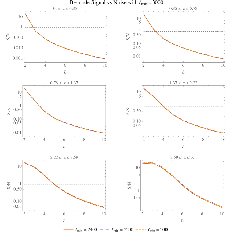
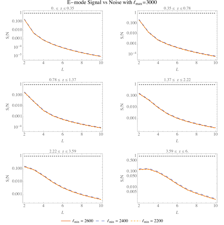
Refer to caption
Figure 5: The signal-to-noise ratio of the B𝐵B-mode estimator b^LMsubscript^𝑏𝐿𝑀\hat{b}_{LM}, equation (4.6), for max=3000subscriptmax3000\ell_{\text{max}}=3000 and six red-shift bins. The optimal value for the filtering scale was chosen numerically, and is given by min=2200subscriptmin2200\ell_{\text{min}}=2200. We find detectability from L=2𝐿2L=2 up to L=3𝐿3L=3 to L=7𝐿7L=7 depending on the red shift bin.
Refer to caption
Figure 6: The signal-to-noise ratio of the E𝐸E-mode estimator e^LMsubscript^𝑒𝐿𝑀\hat{e}_{LM}, equation (4.6), for max=3000subscriptmax3000\ell_{\text{max}}=3000 and six red-shift bins. The optimal value for the filtering scale was chosen numerically, and is given by min=2200subscriptmin2200\ell_{\text{min}}=2200. Unlike for B𝐵B-modes, we do not find detectability for E𝐸E-modes with this value of max=3000subscriptmax3000\ell_{\text{max}}=3000.

In conclusion, there is a signal to detect, and both progress in better sensitivity for future CMB experiments and the use of novel techniques such as intensity mapping to probe the angular matter power spectrum at high resolution will improve the detectability of the signal.

4.3 Information content

Having established the in-principle detectability of a signal, how much would we stand to learn from a detection? To address this, we must examine how correlated we expect the xLM(χ¯e)subscript𝑥𝐿𝑀subscript¯𝜒𝑒x_{LM}(\bar{\chi}_{e}) to be between redshift bins. This is determined by the correlation function of the quadrupole field, eq. (2.39). In figure 7 we show CLqq(χ¯e,χ¯e+δχe)superscriptsubscript𝐶𝐿𝑞𝑞subscript¯𝜒𝑒subscript¯𝜒𝑒𝛿subscript𝜒𝑒C_{L}^{qq}(\bar{\chi}_{e},\bar{\chi}_{e}+\delta\chi_{e}) centered on each of the six redshift bins of table 1 for L=2𝐿2L=2 and L=20𝐿20L=20. Recall that L=2𝐿2L=2 is the lowest non-zero multipole moment, and probes the average quadrupole seen at each redshift. As can be seen from the figure, within ΛΛ\LambdaCDM the L=2𝐿2L=2 moment of the quadrupole field is highly correlated between redshift bins, implying that any one redshift bin contains all of the information about the corresponding modes of the primordial curvature perturbation. On the other hand, the L=20𝐿20L=20 moment of the quadrupole field is relatively uncorrelated between redshift bins, implying that each bin can be used to constrain independent modes.
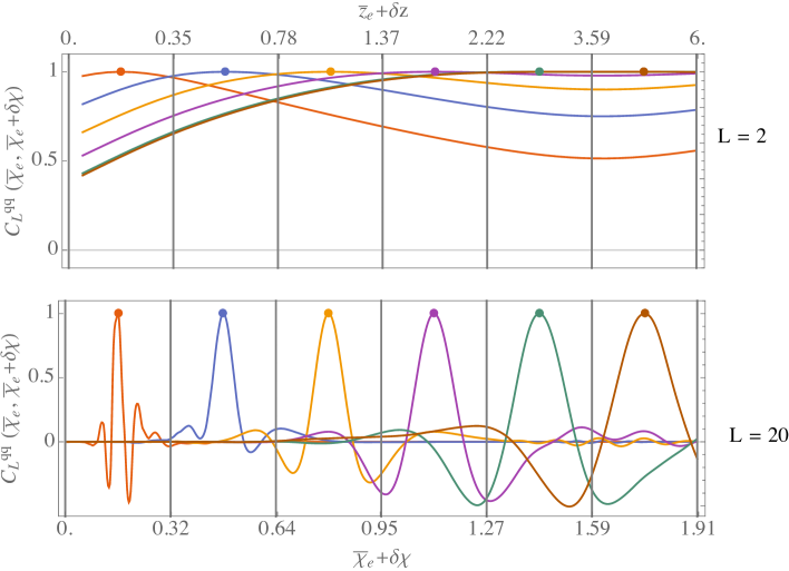
Refer to caption
Figure 7: The effective quadrupole correlation in equation (2.39), normalized as CLqq(χe,χe)[CLqq(χe,χe)CLqq(χe,χe)]1/2superscriptsubscript𝐶𝐿𝑞𝑞subscript𝜒𝑒subscriptsuperscript𝜒𝑒superscriptdelimited-[]superscriptsubscript𝐶𝐿𝑞𝑞subscript𝜒𝑒subscript𝜒𝑒superscriptsubscript𝐶𝐿𝑞𝑞subscriptsuperscript𝜒𝑒subscriptsuperscript𝜒𝑒12C_{L}^{qq}(\chi_{e},\chi^{\prime}_{e})[C_{L}^{qq}(\chi_{e},\chi_{e})C_{L}^{qq}(\chi^{\prime}_{e},\chi^{\prime}_{e})]^{-1/2}, is plotted at χe=χ¯e,χe=χ¯e+δχformulae-sequencesubscript𝜒𝑒subscript¯𝜒𝑒subscriptsuperscript𝜒𝑒subscript¯𝜒𝑒𝛿𝜒\chi_{e}=\bar{\chi}_{e},\ \chi^{\prime}_{e}=\bar{\chi}_{e}+\delta\chi, where χ¯esubscript¯𝜒𝑒\bar{\chi}_{e} is fixed to be the midpoint of a redshift bin. Here, we consider the six evenly spaced redshift bins in table 1 (redshift values displayed along the top axis, comoving distance values displayed along the bottom axis). The different colored curves from left to right fix χ¯e=subscript¯𝜒𝑒absent\bar{\chi}_{e}= 0.16, 0.48, 0.79, 1.11, 1.43, 1.75, in units of H01superscriptsubscript𝐻01H_{0}^{-1}. The top panel shows L=2𝐿2L=2 for which the correlation is important, and the bottom panel shows L=20𝐿20L=20 for which the correlation is less significant within a given redshift bin.

Within a single redshift bin, we can estimate the number of modes as NL=2Lmax2L+1similar-to-or-equals𝑁superscriptsubscript𝐿2subscript𝐿max2𝐿1N\simeq\sum_{L=2}^{L_{\rm max}}2L+1, where Lmaxsubscript𝐿maxL_{\rm max} is the maximum multipole that can be accessed with a SNR of more than one. For the case discussed above, there are as few as 5 modes in the lowest redshift bins and as many as 60 modes in the highest redshift bin detectable using the b𝑏b-mode estimator. However, as discussed above, these modes at low L𝐿L are significantly correlated among redshift bins in ΛΛ\LambdaCDM, and therefore one does not obtain independent measurements from each redshift bin.

There are a few important caveats to add to the discussion above. First, while the correlation among redshift bins at low L𝐿L is not advantageous for constraining a large number of independent modes, it can be used to boost the SNR since the signal in each bin would add coherently. This is equivalent to choosing a different binning scheme for the low L𝐿L moments of the power asymmetry. Second, the degree of correlation between different redshifts is due not only to the fact that the transfer function eq. (2.21) depends mainly on long-wavelength modes, but also our assumption of statistical homogeneity. Violating this assumption, as is invoked to explain many of the existing CMB anomalies, there could be less correlation between redshift bins.

5 Conclusions

In this paper we have demonstrated the ability of polarized Sunyaev Zel’dovich (pSZ) tomography to measure the remote quadrupole field at high signal-to-noise in an idealized, cosmic variance limit. Anisotropy in the remote quadrupole field at each redshift is encoded in an asymmetry in the cross-power between CMB polarization anisotropies and tracers of large scale structure. The quadrupole field is sensitive to structure on the largest possible scales in the observable Universe. Because early-time, high-energy physics is stretched to ultra-large scales, comparable to, or perhaps much larger than, the size of the observable Universe today, pSZ tomography can potentially make a large impact on our understanding of the early Universe 555For example, the analogous observable kSZ tomography can in principle improve the constraints on parameters in various early-Universe cosmologies by orders of magnitude over the CMB alone [5, 6, 7, 8].. Indeed, the first possible hints of beyond-the-standard-cosmological-model physics may have already been detected in the various anomalies in the large scale primary CMB.

Our primary contribution to previous work on this topic has been to set down the general theoretical formalism for pSZ tomography and define a concrete estimator for the quadrupole field. We have made a number of idealized assumptions that could be improved upon. In particular, we have assumed that electrons trace the dark matter, that the density field is Gaussian, that the contribution to the power asymmetry from lensing can be subtracted, that we can neglect systematics such as non-Gaussian and anisotropic instrumental noise, that foregrounds can be subtracted, that we have data on the full sky, a sub-optimal estimator, and possibly other non-idealities. Nevertheless, this work provides a target for future measurements. As we showed in section 4, the next generation of CMB experiments and galaxy surveys have a chance to detect the first few moments of the quadrupole field in a few redshift bins. This fact motivates a more complete forecast for what might be possible.

The potential detection of this signal also motivates a more complete assessment of what we might learn about early Universe physics should such an observation be made. Although it is beyond the scope of the present work, the formalism outlined in this paper can be straightforwardly applied to forecasting parameter constraints on any early-Universe model that makes a prediction for the statistical or deterministic properties of large scale modes of the primordial curvature perturbation. Some targets of potential interest include primordial non-Gaussianity, running of the power spectrum, features in the power spectrum, pre-inflationary inhomogeneities, among other scenarios. We hope to perform detailed forecasts in future work.

Acknowledgments

We thank Gil Holder for important comments and suggestions. MCJ is supported by the National Science and Engineering Research Council through a Discovery grant. AT acknowledges support from the Vanier Canada Graduate Scholarships program. AD is supported by NSF Award PHY-1417385. AD thanks the Perimeter Institute for Theoretical Physics for its hospitality. This research was supported in part by Perimeter Institute for Theoretical Physics. Research at Perimeter Institute is supported by the Government of Canada through the Department of Innovation, Science and Economic Development Canada and by the Province of Ontario through the Ministry of Research, Innovation and Science. Results in this paper were obtained using the HEALPix package [45] (healpix.sourceforge.net) and the Cosmicpy package (cosmicpy.github.io).

Appendix A Fourier Kernel Calculation

In this appendix, we derive the Fourier kernel of the effective quadrupole (eq. (2.14),(2.15)). Each contribution is treated one at a time. Let’s begin with the Sachs-Wolfe contribution. Substituting equation (2.13) and (2.7) into (2.6) yields

qSWm(𝐧^e,χe)=(2DΨ(χdec)32)Ωd2𝐧^d3k(2π)3Ψ~i(𝐤)eiχe𝐤𝐧^eeiΔχdec𝐤𝐧^Y2m(𝐧^).superscriptsubscript𝑞SW𝑚subscript^𝐧𝑒subscript𝜒𝑒2subscript𝐷Ψsubscript𝜒dec32subscriptΩsuperscript𝑑2^𝐧superscript𝑑3𝑘superscript2𝜋3subscript~Ψ𝑖𝐤superscript𝑒𝑖subscript𝜒𝑒𝐤subscript^𝐧𝑒superscript𝑒𝑖Δsubscript𝜒dec𝐤^𝐧subscriptsuperscript𝑌2𝑚^𝐧q_{\text{SW}}^{m}({\bf\hat{n}}_{e},\chi_{e})=\left(2D_{\Psi}(\chi_{\text{dec}})-\frac{3}{2}\right)\int_{\Omega}d^{2}{\bf\hat{n}}\int\frac{d^{3}k}{(2\pi)^{3}}\tilde{\Psi}_{i}({\bf k})e^{i\chi_{e}{\bf k}\cdot{\bf\hat{n}}_{e}}e^{i\Delta\chi_{\text{dec}}{\bf k}\cdot{\bf\hat{n}}}\ Y^{*}_{2m}({\bf\hat{n}}). (A.1)

Next, we employ the identity for the expansion of the exponential,

eiΔχ𝐤𝐧^=,m4πij(kΔχ)Ym(𝐤^)Ym(𝐧^),superscript𝑒𝑖Δ𝜒𝐤^𝐧subscriptsuperscriptsuperscript𝑚4𝜋superscript𝑖superscriptsubscript𝑗superscript𝑘Δ𝜒subscriptsuperscript𝑌superscriptsuperscript𝑚^𝐤subscript𝑌superscriptsuperscript𝑚^𝐧e^{i\Delta\chi{\bf k}\cdot{\bf\hat{n}}}=\sum_{\ell^{\prime},m^{\prime}}4\pi\ i^{\ell^{\prime}}\ j_{\ell^{\prime}}(k\Delta\chi)\ Y^{*}_{\ell^{\prime}m^{\prime}}({\bf\hat{k}})Y_{\ell^{\prime}m^{\prime}}({\bf\hat{n}}), (A.2)

resulting in,

qSWm(𝐧^e,χe)=superscriptsubscript𝑞SW𝑚subscript^𝐧𝑒subscript𝜒𝑒absent\displaystyle q_{\text{SW}}^{m}({\bf\hat{n}}_{e},\chi_{e})= d3k(2π)3Ψ~i(𝐤)(2DΨ(χdec)32)superscript𝑑3𝑘superscript2𝜋3subscript~Ψ𝑖𝐤2subscript𝐷Ψsubscript𝜒dec32\displaystyle\int\frac{d^{3}k}{(2\pi)^{3}}\tilde{\Psi}_{i}({\bf k})\left(2D_{\Psi}(\chi_{\text{dec}})-\frac{3}{2}\right) (A.3)
×Ωd2𝐧^,m4πij(kΔχdec)Ym(𝐤^)Ym(𝐧^)Y2m(𝐧^)eiχe𝐤𝐧^e\displaystyle\times\int_{\Omega}d^{2}{\bf\hat{n}}\sum_{\ell^{\prime},m^{\prime}}4\pi\ i^{\ell^{\prime}}j_{\ell^{\prime}}(k\Delta\chi_{\text{dec}})\ Y^{*}_{\ell^{\prime}m^{\prime}}({\bf\hat{k}})Y_{\ell^{\prime}m^{\prime}}({\bf\hat{n}})\ Y^{*}_{2m}({\bf\hat{n}})e^{i\chi_{e}{\bf k}\cdot{\bf\hat{n}}_{e}}
=\displaystyle= d3k(2π)3Ψ~i(𝐤)[4π(2DΨ(χdec)32)j2(kΔχdec)]Y2m(𝐤^)eiχe𝐤𝐧^e,superscript𝑑3𝑘superscript2𝜋3subscript~Ψ𝑖𝐤delimited-[]4𝜋2subscript𝐷Ψsubscript𝜒dec32subscript𝑗2𝑘Δsubscript𝜒decsubscriptsuperscript𝑌2𝑚^𝐤superscript𝑒𝑖subscript𝜒𝑒𝐤subscript^𝐧𝑒\displaystyle\int\frac{d^{3}k}{(2\pi)^{3}}\tilde{\Psi}_{i}({\bf k})\left[-4\pi\left(2D_{\Psi}(\chi_{\text{dec}})-\frac{3}{2}\right)j_{2}(k\Delta\chi_{\text{dec}})\right]Y^{*}_{2m}({\bf\hat{k}})e^{i\chi_{e}{\bf k}\cdot{\bf\hat{n}}_{e}}, (A.4)

where we integrated over 𝐧^^𝐧\hat{\bf n} to obtain δ2δmmsubscript𝛿superscript2subscript𝛿superscript𝑚𝑚\delta_{\ell^{\prime}2}\delta_{m^{\prime}m}.

The steps of the calculation are identical for the integrated Sachs-Wolfe term. We start with ΘISWsubscriptΘISW\Theta_{\text{ISW}} in eq. (2.8) to obtain the resulting contribution:

qISWm(𝐧^e,χe)superscriptsubscript𝑞ISW𝑚subscript^𝐧𝑒subscript𝜒𝑒\displaystyle q_{\text{ISW}}^{m}({\bf\hat{n}}_{e},\chi_{e}) =2Ωd2𝐧^adecae𝑑adDΨdad3k(2π)3Ψ~i(𝐤)eiχe𝐤𝐧^eeiΔχ(a)𝐤𝐧^Y2m(𝐧^)absent2subscriptΩsuperscript𝑑2^𝐧superscriptsubscriptsubscript𝑎decsubscript𝑎𝑒differential-d𝑎𝑑subscript𝐷Ψ𝑑𝑎superscript𝑑3𝑘superscript2𝜋3subscript~Ψ𝑖𝐤superscript𝑒𝑖subscript𝜒𝑒𝐤subscript^𝐧𝑒superscript𝑒𝑖Δ𝜒𝑎𝐤^𝐧subscriptsuperscript𝑌2𝑚^𝐧\displaystyle=2\int_{\Omega}d^{2}{\bf\hat{n}}\int_{a_{\rm dec}}^{a_{e}}da\frac{dD_{\Psi}}{da}\int\frac{d^{3}k}{(2\pi)^{3}}\tilde{\Psi}_{i}({\bf k})e^{i\chi_{e}{\bf k}\cdot{\bf\hat{n}}_{e}}e^{i\Delta\chi(a){\bf k}\cdot{\bf\hat{n}}}\ Y^{*}_{2m}({\bf\hat{n}})
=2d3k(2π)3Ψ~i(𝐤)adecae𝑑adDΨdaΩd2𝐧^,m4πij(kΔχ(a))absent2superscript𝑑3𝑘superscript2𝜋3subscript~Ψ𝑖𝐤superscriptsubscriptsubscript𝑎decsubscript𝑎𝑒differential-d𝑎𝑑subscript𝐷Ψ𝑑𝑎subscriptΩsuperscript𝑑2^𝐧subscriptsuperscriptsuperscript𝑚4𝜋superscript𝑖superscriptsubscript𝑗superscript𝑘Δ𝜒𝑎\displaystyle=2\int\frac{d^{3}k}{(2\pi)^{3}}\tilde{\Psi}_{i}({\bf k})\int_{a_{\rm dec}}^{a_{e}}da\frac{dD_{\Psi}}{da}\int_{\Omega}d^{2}{\bf\hat{n}}\sum_{\ell^{\prime},m^{\prime}}4\pi\ i^{\ell^{\prime}}j_{\ell^{\prime}}(k\Delta\chi(a))
×Ym(𝐤^)Ym(𝐧^)Y2m(𝐧^)eiχe𝐤𝐧^eabsentsubscriptsuperscript𝑌superscriptsuperscript𝑚^𝐤subscript𝑌superscriptsuperscript𝑚^𝐧subscriptsuperscript𝑌2𝑚^𝐧superscript𝑒𝑖subscript𝜒𝑒𝐤subscript^𝐧𝑒\displaystyle\quad\times Y^{*}_{\ell^{\prime}m^{\prime}}({\bf\hat{k}})\ Y_{\ell^{\prime}m^{\prime}}({\bf\hat{n}})\ Y^{*}_{2m}({\bf\hat{n}})\ e^{i\chi_{e}{\bf k}\cdot{\bf\hat{n}}_{e}}
=d3k(2π)3Ψ~i(𝐤)[8πadecae𝑑adDΨdaj2(kΔχ(a))]Y2m(𝐤^)eiχe𝐤𝐧^e.absentsuperscript𝑑3𝑘superscript2𝜋3subscript~Ψ𝑖𝐤delimited-[]8𝜋superscriptsubscriptsubscript𝑎decsubscript𝑎𝑒differential-d𝑎𝑑subscript𝐷Ψ𝑑𝑎subscript𝑗2𝑘Δ𝜒𝑎subscriptsuperscript𝑌2𝑚^𝐤superscript𝑒𝑖subscript𝜒𝑒𝐤subscript^𝐧𝑒\displaystyle=\int\frac{d^{3}k}{(2\pi)^{3}}\tilde{\Psi}_{i}({\bf k})\left[-8\pi\int_{a_{\rm dec}}^{a_{e}}da\frac{dD_{\Psi}}{da}\ j_{2}(k\Delta\chi(a))\right]Y^{*}_{2m}({\bf\hat{k}})e^{i\chi_{e}{\bf k}\cdot{\bf\hat{n}}_{e}}. (A.5)

Both the SW and ISW contributions are sensitive mainly to large scale potential fluctuations, as shown in figure 2.

The derivation of the Doppler kernel requires more work. However, the contribution from the second term in eq. (2.9) vanishes. To show this, we substitute the second term of ΘDopplersubscriptΘDoppler\Theta_{\text{Doppler}} into the effective quadrupole, yielding,

Dv(χe)Ωd2𝐧^d3k(2π)3ikΨ~i(𝐤)(𝐧^𝐤^)eiχe𝐤𝐧^eY2m(𝐧^).subscript𝐷𝑣subscript𝜒𝑒subscriptΩsuperscript𝑑2^𝐧superscript𝑑3𝑘superscript2𝜋3𝑖𝑘subscript~Ψ𝑖𝐤^𝐧^𝐤superscript𝑒𝑖subscript𝜒𝑒𝐤subscript^𝐧𝑒subscriptsuperscript𝑌2𝑚^𝐧-D_{v}(\chi_{e})\int_{\Omega}d^{2}{\bf\hat{n}}\int\frac{d^{3}k}{(2\pi)^{3}}\ ik\tilde{\Psi}_{i}({\bf k})(\hat{\bf n}\cdot\hat{\bf k})e^{i\chi_{e}{\bf k}\cdot{\bf\hat{n}}_{e}}\ Y^{*}_{2m}({\bf\hat{n}}). (A.6)

It is equivalent to write (𝐧^𝐤^)^𝐧^𝐤(\hat{\bf n}\cdot\hat{\bf k}) as 𝒫1(𝐧^𝐤^)subscript𝒫1^𝐧^𝐤\mathcal{P}_{1}(\hat{\bf n}\cdot\hat{\bf k}) and then expand the Legendre polynomial in terms of spherical harmonics using

𝒫(𝐱^𝐱^)=4π2+1m=Ym(𝐱^)Ym(𝐱^).subscript𝒫^𝐱superscript^𝐱4𝜋21superscriptsubscript𝑚subscriptsuperscript𝑌𝑚^𝐱subscript𝑌𝑚superscript^𝐱\mathcal{P}_{\ell}({\bf\hat{x}}\cdot{\bf\hat{x}}^{\prime})=\frac{4\pi}{2\ell+1}\sum_{m=-\ell}^{\ell}Y^{*}_{\ell m}({\bf\hat{x}})\ Y_{\ell m}({\bf\hat{x}}^{\prime}). (A.7)

Doing so results in

Dv(χe)d3k(2π)3ikΨ~i(𝐤)eiχe𝐤𝐧^eΩd2𝐧^4π3m=11Y1m(𝐤^)Y1m(𝐧^)Y2m(𝐧^)=0,subscript𝐷𝑣subscript𝜒𝑒superscript𝑑3𝑘superscript2𝜋3𝑖𝑘subscript~Ψ𝑖𝐤superscript𝑒𝑖subscript𝜒𝑒𝐤subscript^𝐧𝑒subscriptΩsuperscript𝑑2^𝐧4𝜋3superscriptsubscriptsuperscript𝑚11subscriptsuperscript𝑌1superscript𝑚^𝐤subscript𝑌1superscript𝑚^𝐧subscriptsuperscript𝑌2𝑚^𝐧0-D_{v}(\chi_{e})\int\frac{d^{3}k}{(2\pi)^{3}}\ ik\tilde{\Psi}_{i}({\bf k})e^{i\chi_{e}{\bf k}\cdot{\bf\hat{n}}_{e}}\int_{\Omega}d^{2}{\bf\hat{n}}\ \frac{4\pi}{3}\sum_{m^{\prime}=-1}^{1}Y^{*}_{1m^{\prime}}({\bf\hat{k}})\ Y_{1m^{\prime}}({\bf\hat{n}})Y^{*}_{2m}({\bf\hat{n}})=0, (A.8)

which vanishes upon integration over 𝐧^^𝐧\hat{\bf n} due to the orthogonality of the spherical harmonics. The first term of eq. (2.9) gives a non-zero contribution to the effective quadrupole. The calculation proceeds similarly, except for the additional factor of eiΔχdec𝐤𝐧^superscript𝑒𝑖Δsubscript𝜒dec𝐤^𝐧e^{i\Delta\chi_{\text{dec}}{\bf k}\cdot{\bf\hat{n}}} which needs to be expanded using (A.2):

qDopplerm(𝐧^e,χe)superscriptsubscript𝑞Doppler𝑚subscript^𝐧𝑒subscript𝜒𝑒\displaystyle q_{\text{Doppler}}^{m}({\bf\hat{n}}_{e},\chi_{e}) =Dv(χdec)Ωd2𝐧^d3k(2π)3ikΨ~i(𝐤)(𝐧^𝐤^)eiχe𝐤𝐧^eeiΔχdec𝐤𝐧^Y2m(𝐧^)absentsubscript𝐷𝑣subscript𝜒decsubscriptΩsuperscript𝑑2^𝐧superscript𝑑3𝑘superscript2𝜋3𝑖𝑘subscript~Ψ𝑖𝐤^𝐧^𝐤superscript𝑒𝑖subscript𝜒𝑒𝐤subscript^𝐧𝑒superscript𝑒𝑖Δsubscript𝜒dec𝐤^𝐧subscriptsuperscript𝑌2𝑚^𝐧\displaystyle=D_{v}(\chi_{\text{dec}})\int_{\Omega}d^{2}{\bf\hat{n}}\int\frac{d^{3}k}{(2\pi)^{3}}\ ik\tilde{\Psi}_{i}({\bf k})(\hat{\bf n}\cdot\hat{\bf k})e^{i\chi_{e}{\bf k}\cdot{\bf\hat{n}}_{e}}e^{i\Delta\chi_{\text{dec}}{\bf k}\cdot{\bf\hat{n}}}\ Y^{*}_{2m}({\bf\hat{n}})
=Dv(χdec)Ωd2𝐧^d3k(2π)3ikΨ~i(𝐤)4π3m=11Y1m(𝐤^)Y1m(𝐧^)×′′,m′′4πi′′j′′(kΔχ(a))Y′′m′′(𝐤^)Y′′m′′(𝐧^)eiχe𝐤𝐧^eY2m(𝐧^).absentsubscript𝐷𝑣subscript𝜒decsubscriptΩsuperscript𝑑2^𝐧superscript𝑑3𝑘superscript2𝜋3𝑖𝑘subscript~Ψ𝑖𝐤4𝜋3superscriptsubscriptsuperscript𝑚11subscriptsuperscript𝑌1superscript𝑚^𝐤subscript𝑌1superscript𝑚^𝐧subscriptsuperscript′′superscript𝑚′′4𝜋superscript𝑖superscript′′subscript𝑗superscript′′𝑘Δ𝜒𝑎subscriptsuperscript𝑌superscript′′superscript𝑚′′^𝐤subscript𝑌superscript′′superscript𝑚′′^𝐧superscript𝑒𝑖subscript𝜒𝑒𝐤subscript^𝐧𝑒subscriptsuperscript𝑌2𝑚^𝐧\displaystyle\begin{split}&=D_{v}(\chi_{\text{dec}})\int_{\Omega}d^{2}{\bf\hat{n}}\int\frac{d^{3}k}{(2\pi)^{3}}\ ik\tilde{\Psi}_{i}({\bf k})\ \frac{4\pi}{3}\sum_{m^{\prime}=-1}^{1}Y^{*}_{1m^{\prime}}({\bf\hat{k}})\ Y_{1m^{\prime}}({\bf\hat{n}})\\ &\quad\times\sum_{\ell^{\prime\prime},m^{\prime\prime}}4\pi\ i^{\ell^{\prime\prime}}j_{\ell^{\prime\prime}}(k\Delta\chi(a))\ Y^{*}_{\ell^{\prime\prime}m^{\prime\prime}}({\bf\hat{k}})Y_{\ell^{\prime\prime}m^{\prime\prime}}({\bf\hat{n}})e^{i\chi_{e}{\bf k}\cdot{\bf\hat{n}}_{e}}\ Y^{*}_{2m}({\bf\hat{n}}).\end{split} (A.9)

In the above expression, the integral over 𝐧^^𝐧\hat{\bf n} is a triple product of spherical harmonics. For this we can apply the general identity in terms of Wigner 3-j𝑗j symbols,

Ωd2𝐧^Y1m1s1(𝐧^)Y2m2s2(𝐧^)Y3m3s3(𝐧^)=(21+1)(22+1)(23+1)4π×(123m1m2m3)(123s1s2s3)subscriptΩsuperscript𝑑2^𝐧subscriptsubscript𝑌subscript1subscript𝑚1subscript𝑠1^𝐧subscriptsubscript𝑌subscript2subscript𝑚2subscript𝑠2^𝐧subscriptsubscript𝑌subscript3subscript𝑚3subscript𝑠3^𝐧2subscript112subscript212subscript314𝜋subscript1subscript2subscript3subscript𝑚1subscript𝑚2subscript𝑚3subscript1subscript2subscript3subscript𝑠1subscript𝑠2subscript𝑠3\begin{split}\int_{\Omega}d^{2}{\bf\hat{n}}\ {}_{s_{1}}Y_{\ell_{1}m_{1}}({\bf\hat{n}}){}_{s_{2}}Y_{\ell_{2}m_{2}}({\bf\hat{n}}){}_{s_{3}}Y_{\ell_{3}m_{3}}({\bf\hat{n}})&=\sqrt{\frac{(2\ell_{1}+1)(2\ell_{2}+1)(2\ell_{3}+1)}{4\pi}}\\ &\quad\times\left(\begin{array}[]{ccc}\ell_{1}&\ell_{2}&\ell_{3}\\ m_{1}&m_{2}&m_{3}\end{array}\right)\left(\begin{array}[]{ccc}\ell_{1}&\ell_{2}&\ell_{3}\\ -s_{1}&-s_{2}&-s_{3}\end{array}\right)\end{split} (A.10)

with spin weights s1=s2=s3=0subscript𝑠1subscript𝑠2subscript𝑠30s_{1}=s_{2}=s_{3}=0. There are also two spherical harmonics with argument 𝐤^^𝐤\hat{\bf k} that can be expressed as a single spherical harmonic using another identity,

Y1m1s1(𝐧^)Y2m2s2(𝐧^)=S,L,M(1)1+2+L(21+1)(22+1)(2L+1)4π×(12Lm1m2M)(12Ls1s2S)YLMS(𝐧^).subscriptsubscript𝑌subscript1subscript𝑚1subscript𝑠1^𝐧subscriptsubscript𝑌subscript2subscript𝑚2subscript𝑠2^𝐧subscript𝑆𝐿𝑀superscript1subscript1subscript2𝐿2subscript112subscript212𝐿14𝜋subscript1subscript2𝐿subscript𝑚1subscript𝑚2𝑀subscript1subscript2𝐿subscript𝑠1subscript𝑠2𝑆subscriptsuperscriptsubscript𝑌𝐿𝑀𝑆^𝐧\begin{split}{}_{s_{1}}Y_{\ell_{1}m_{1}}({\bf\hat{n}})\ {}_{s_{2}}Y_{\ell_{2}m_{2}}({\bf\hat{n}})=\sum_{S,L,M}&(-1)^{\ell_{1}+\ell_{2}+L}\sqrt{\frac{(2\ell_{1}+1)(2\ell_{2}+1)(2L+1)}{4\pi}}\\ &\quad\times\left(\begin{array}[]{ccc}\ell_{1}&\ell_{2}&L\\ m_{1}&m_{2}&M\end{array}\right)\left(\begin{array}[]{ccc}\ell_{1}&\ell_{2}&L\\ s_{1}&s_{2}&S\end{array}\right){}_{S}Y_{LM}^{*}({\bf\hat{n}}).\end{split} (A.11)

Putting all of this together yields

qDopplerm(𝐧^e,χe)superscriptsubscript𝑞Doppler𝑚subscript^𝐧𝑒subscript𝜒𝑒\displaystyle q_{\text{Doppler}}^{m}({\bf\hat{n}}_{e},\chi_{e}) =Dv(χdec)d3k(2π)3ikΨ~i(𝐤)L,M,m,′′,m′′(5)(3)(2′′+1)4πabsentsubscript𝐷𝑣subscript𝜒decsuperscript𝑑3𝑘superscript2𝜋3𝑖𝑘subscript~Ψ𝑖𝐤subscript𝐿𝑀superscript𝑚superscript′′superscript𝑚′′532superscript′′14𝜋\displaystyle=D_{v}(\chi_{\text{dec}})\int\frac{d^{3}k}{(2\pi)^{3}}\ ik\tilde{\Psi}_{i}({\bf k})\sum_{\begin{subarray}{c}L,M,m^{\prime},\\ \ell^{\prime\prime},m^{\prime\prime}\end{subarray}}\sqrt{\frac{(5)(3)(2\ell^{\prime\prime}+1)}{4\pi}}
×(2L+1)(3)(2′′+1)4π(4π)23i′′j′′(kΔχdec)(1)′′+L+1absent2𝐿132superscript′′14𝜋superscript4𝜋23superscript𝑖superscript′′subscript𝑗superscript′′𝑘Δsubscript𝜒decsuperscript1superscript′′𝐿1\displaystyle\quad\times\sqrt{\frac{(2L+1)(3)(2\ell^{\prime\prime}+1)}{4\pi}}\frac{(4\pi)^{2}}{3}i^{\ell^{\prime\prime}}j_{\ell^{\prime\prime}}(k\Delta\chi_{\text{dec}})(-1)^{\ell^{\prime\prime}+L+1} (A.12)
×(1′′Lmm′′M)(21′′mmm′′)(21′′000)(1′′L000)YLM(𝐤^)eiχe𝐤𝐧^e.absent1superscript′′𝐿superscript𝑚superscript𝑚′′𝑀21superscript′′𝑚superscript𝑚superscript𝑚′′21superscript′′0001superscript′′𝐿000subscriptsuperscript𝑌𝐿𝑀^𝐤superscript𝑒𝑖subscript𝜒𝑒𝐤subscript^𝐧𝑒\displaystyle\quad\times\left(\begin{array}[]{ccc}1&\ell^{\prime\prime}&L\\ m^{\prime}&m^{\prime\prime}&M\end{array}\right)\left(\begin{array}[]{ccc}2&1&\ell^{\prime\prime}\\ m&m^{\prime}&m^{\prime\prime}\end{array}\right)\left(\begin{array}[]{ccc}2&1&\ell^{\prime\prime}\\ 0&0&0\end{array}\right)\left(\begin{array}[]{ccc}1&\ell^{\prime\prime}&L\\ 0&0&0\end{array}\right)Y^{*}_{LM}({\bf\hat{k}})e^{i\chi_{e}{\bf k}\cdot{\bf\hat{n}}_{e}}. (A.21)

Fortunately, the sum over m′′superscript𝑚′′m^{\prime\prime} and msuperscript𝑚m^{\prime} simplify the expression drastically because of the orthogonality relation,

m1,m2(12Lm1m2M)(12Lm1m2M)=δLLδMM2L+1.subscriptsubscript𝑚1subscript𝑚2subscript1subscript2𝐿subscript𝑚1subscript𝑚2𝑀subscript1subscript2superscript𝐿subscript𝑚1subscript𝑚2superscript𝑀subscript𝛿𝐿superscript𝐿subscript𝛿𝑀superscript𝑀2𝐿1\sum_{m_{1},m_{2}}\left(\begin{array}[]{ccc}\ell_{1}&\ell_{2}&L\\ m_{1}&m_{2}&M\end{array}\right)\left(\begin{array}[]{ccc}\ell_{1}&\ell_{2}&L^{\prime}\\ m_{1}&m_{2}&M^{\prime}\end{array}\right)=\frac{\delta_{LL^{\prime}}\delta_{MM^{\prime}}}{2L+1}. (A.22)

Using the invariance of the Wigner 3-j𝑗j symbols under even permutations of its columns, we can apply this relation to the first two 3-j𝑗j symbols in eq. (A.12), it follows that,

qDopplerm(𝐧^e,χe)=Dv(χdec)d3k(2π)3ikΨ~i(𝐤)′′4πi′′j′′(kΔχdec)×(1)′′+1(2′′+1)(21′′000)2Y2m(𝐤^)eiχe𝐤𝐧^e.superscriptsubscript𝑞Doppler𝑚subscript^𝐧𝑒subscript𝜒𝑒subscript𝐷𝑣subscript𝜒decsuperscript𝑑3𝑘superscript2𝜋3𝑖𝑘subscript~Ψ𝑖𝐤subscriptsuperscript′′4𝜋superscript𝑖superscript′′subscript𝑗superscript′′𝑘Δsubscript𝜒decsuperscript1superscript′′12superscript′′1superscript21superscript′′0002subscriptsuperscript𝑌2𝑚^𝐤superscript𝑒𝑖subscript𝜒𝑒𝐤subscript^𝐧𝑒\begin{split}q_{\text{Doppler}}^{m}({\bf\hat{n}}_{e},\chi_{e})&=D_{v}(\chi_{\text{dec}})\int\frac{d^{3}k}{(2\pi)^{3}}\ ik\tilde{\Psi}_{i}({\bf k})\sum_{\ell^{\prime\prime}}4\pi i^{\ell^{\prime\prime}}j_{\ell^{\prime\prime}}(k\Delta\chi_{\text{dec}})\\ &\quad\times(-1)^{\ell^{\prime\prime}+1}(2\ell^{\prime\prime}+1)\left(\begin{array}[]{ccc}2&1&\ell^{\prime\prime}\\ 0&0&0\end{array}\right)^{2}Y^{*}_{2m}({\bf\hat{k}})e^{i\chi_{e}{\bf k}\cdot{\bf\hat{n}}_{e}}.\end{split} (A.23)

The remaining 3-j𝑗j symbol is only non-zero for ′′=superscript′′absent\ell^{\prime\prime}= 1 and 3, resulting in the final expression for the Doppler contribution,

qDopplerm(𝐧^e,χe)=superscriptsubscript𝑞Doppler𝑚subscript^𝐧𝑒subscript𝜒𝑒absent\displaystyle q_{\text{Doppler}}^{m}({\bf\hat{n}}_{e},\chi_{e})= d3k(2π)3Ψ~i(𝐤)×Y2m(𝐤^)eiχe𝐤𝐧^esuperscript𝑑3𝑘superscript2𝜋3subscript~Ψ𝑖𝐤subscriptsuperscript𝑌2𝑚^𝐤superscript𝑒𝑖subscript𝜒𝑒𝐤subscript^𝐧𝑒\displaystyle\int\frac{d^{3}k}{(2\pi)^{3}}\tilde{\Psi}_{i}({\bf k})\times Y^{*}_{2m}({\bf\hat{k}})e^{i\chi_{e}{\bf k}\cdot{\bf\hat{n}}_{e}}
×[4π5kDv(χdec)(3j3(kΔχdec)2j1(kΔχdec))].absentdelimited-[]4𝜋5𝑘subscript𝐷𝑣subscript𝜒dec3subscript𝑗3𝑘Δsubscript𝜒dec2subscript𝑗1𝑘Δsubscript𝜒dec\displaystyle\times\left[\frac{4\pi}{5}kD_{v}(\chi_{\text{dec}})\left(3j_{3}(k\Delta\chi_{\text{dec}})-2j_{1}(k\Delta\chi_{\text{dec}})\right)\right]. (A.24)

As illustrated in figure 2, the Doppler term dominates over SW and ISW contributions on small scales k20H0greater-than-or-equivalent-to𝑘20subscript𝐻0k\gtrsim 20H_{0}.

The full expression for the effective quadrupole is a sum of the contributions in (A.4), (A.5) and (A.24):

qeffm(𝐧^e,χe)=d3k(2π)3Ψ~i(𝐤)T(k)[𝒢SW+𝒢ISW+𝒢Doppler]Y2m(𝐤^)eiχe𝐤𝐧^e,subscriptsuperscript𝑞𝑚effsubscript^𝐧𝑒subscript𝜒𝑒superscript𝑑3𝑘superscript2𝜋3subscript~Ψ𝑖𝐤𝑇𝑘delimited-[]subscript𝒢SWsubscript𝒢ISWsubscript𝒢Dopplersuperscriptsubscript𝑌2𝑚^𝐤superscript𝑒𝑖subscript𝜒𝑒𝐤subscript^𝐧𝑒q^{m}_{\rm eff}({\bf\hat{n}}_{e},\chi_{e})=\int\frac{d^{3}k}{(2\pi)^{3}}\tilde{\Psi}_{i}({\bf k})T(k)\left[\mathcal{G}_{\rm SW}+\mathcal{G}_{\rm ISW}+\mathcal{G}_{\rm Doppler}\right]Y_{2m}^{*}({\bf\hat{k}})\ e^{i\chi_{e}{\bf k}\cdot{\bf\hat{n}}_{e}}, (A.25)

where we have added the transfer function T(k)𝑇𝑘T(k) which has the form given in (2.16), and the kernels 𝒢SWsubscript𝒢SW\mathcal{G}_{\rm SW}, 𝒢ISWsubscript𝒢ISW\mathcal{G}_{\rm ISW} and 𝒢Dopplersubscript𝒢Doppler\mathcal{G}_{\rm Doppler} are given by,

𝒢SW(k,χe)subscript𝒢SW𝑘subscript𝜒𝑒\displaystyle\mathcal{G}_{\rm SW}(k,\chi_{e}) =4π(2DΨ(χdec)32)j2(kΔχdec),absent4𝜋2subscript𝐷Ψsubscript𝜒dec32subscript𝑗2𝑘Δsubscript𝜒dec\displaystyle=-4\pi\left(2D_{\Psi}(\chi_{\rm dec})-\frac{3}{2}\right)j_{2}(k\Delta\chi_{\text{dec}}),
𝒢ISW(k,χe)subscript𝒢ISW𝑘subscript𝜒𝑒\displaystyle\mathcal{G}_{\rm ISW}(k,\chi_{e}) =8πadecae𝑑adDΨdaj2(kΔχ(a)),absent8𝜋superscriptsubscriptsubscript𝑎decsubscript𝑎𝑒differential-d𝑎𝑑subscript𝐷Ψ𝑑𝑎subscript𝑗2𝑘Δ𝜒𝑎\displaystyle=-8\pi\int_{a_{\rm dec}}^{a_{e}}da\frac{dD_{\Psi}}{da}\ j_{2}(k\Delta\chi(a)),
𝒢Doppler(k,χe)subscript𝒢Doppler𝑘subscript𝜒𝑒\displaystyle\mathcal{G}_{\rm Doppler}(k,\chi_{e}) =4π5kDv(χdec)[3j3(kΔχdec)2j1(kΔχdec)].absent4𝜋5𝑘subscript𝐷𝑣subscript𝜒decdelimited-[]3subscript𝑗3𝑘Δsubscript𝜒dec2subscript𝑗1𝑘Δsubscript𝜒dec\displaystyle=\frac{4\pi}{5}kD_{v}(\chi_{\text{dec}})\left[3j_{3}(k\Delta\chi_{\text{dec}})-2j_{1}(k\Delta\chi_{\text{dec}})\right]. (A.26)

Appendix B Multipole coefficients for the total effective quadrupole

Here we compute amq(χe)superscriptsubscript𝑎𝑚𝑞subscript𝜒𝑒a_{\ell m}^{q}(\chi_{e}) starting from (2.19). Inserting the total effective quadrupole (2.17) and the expression for qeffmsuperscriptsubscript𝑞eff𝑚q_{\text{eff}}^{m} from (2.14), we have

amq(χe)=Ωd2𝐧^em=22d3k(2π)3Ψ~i(𝐤)T(k)[𝒢SW+𝒢ISW+𝒢Doppler]×Y2m(𝐤^)eiχe𝐤𝐧^eY2m±2(𝐧^e)Ym±2(𝐧^e).superscriptsubscript𝑎𝑚𝑞subscript𝜒𝑒subscriptΩsuperscript𝑑2subscript^𝐧𝑒superscriptsubscriptsuperscript𝑚22superscript𝑑3𝑘superscript2𝜋3subscript~Ψ𝑖𝐤𝑇𝑘delimited-[]subscript𝒢SWsubscript𝒢ISWsubscript𝒢Dopplersuperscriptsubscript𝑌2superscript𝑚^𝐤superscript𝑒𝑖subscript𝜒𝑒𝐤subscript^𝐧𝑒subscriptsubscript𝑌2superscript𝑚plus-or-minus2subscript^𝐧𝑒subscriptsubscriptsuperscript𝑌𝑚plus-or-minus2subscript^𝐧𝑒\begin{split}a_{\ell m}^{q}(\chi_{e})&=\int_{\Omega}d^{2}{\bf\hat{n}}_{e}\sum_{m^{\prime}=-2}^{2}\int\frac{d^{3}k}{(2\pi)^{3}}\tilde{\Psi}_{i}({\bf k})T(k)\left[\mathcal{G}_{\rm SW}+\mathcal{G}_{\rm ISW}+\mathcal{G}_{\rm Doppler}\right]\\ &\quad\times Y_{2m^{\prime}}^{*}({\bf\hat{k}})\ e^{i\chi_{e}{\bf k}\cdot{\bf\hat{n}}_{e}}\left.{}_{\pm 2}Y_{2m^{\prime}}\right.({\bf\hat{n}}_{e})\left.{}_{\pm 2}Y^{*}_{\ell m}\right.({\bf\hat{n}}_{e})\ .\end{split} (B.1)

When we expand the exponential with the exponential identity (A.2) introducing new multipole parameters L,M𝐿𝑀L,\ M, there will be five spherical harmonics, three with argument 𝐧^esubscript^𝐧𝑒{\bf\hat{n}}_{e}: Y2m±2(𝐧^e),Ym±2(𝐧^e)subscriptsubscript𝑌2superscript𝑚plus-or-minus2subscript^𝐧𝑒subscriptsubscriptsuperscript𝑌𝑚plus-or-minus2subscript^𝐧𝑒\left.{}_{\pm 2}Y_{2m^{\prime}}\right.({\bf\hat{n}}_{e}),\left.{}_{\pm 2}Y^{*}_{\ell m}\right.({\bf\hat{n}}_{e}) and YLM(𝐧^e)subscript𝑌𝐿𝑀subscript^𝐧𝑒Y_{LM}({\bf\hat{n}}_{e}), and two with argument 𝐤^^𝐤{\bf\hat{k}}: Y2m(𝐤^)superscriptsubscript𝑌2superscript𝑚^𝐤Y_{2m^{\prime}}^{*}({\bf\hat{k}}) and YLM(𝐤^)superscriptsubscript𝑌𝐿𝑀^𝐤Y_{LM}^{*}({\bf\hat{k}}). The first three can be handled by the triple-product spin-weighted spherical harmonic integral identity in eq. (A.10). Using this to integrate the spherical harmonics with argument 𝐧^esubscript^𝐧𝑒{\bf\hat{n}}_{e} gives

Ωd2𝐧^Y2m±2(𝐧^e)Ym±2(𝐧^e)YLM(𝐧^e)=(1)m(5)(2+1)(2L+1)4π×(2LmmM)(2L±220).subscriptΩsuperscript𝑑2^𝐧subscriptsubscript𝑌2superscript𝑚plus-or-minus2subscript^𝐧𝑒subscriptsubscriptsuperscript𝑌𝑚plus-or-minus2subscript^𝐧𝑒subscript𝑌𝐿𝑀subscript^𝐧𝑒superscript1𝑚5212𝐿14𝜋2𝐿𝑚superscript𝑚𝑀2𝐿plus-or-minus2minus-or-plus20\begin{split}\int_{\Omega}d^{2}{\bf\hat{n}}\ \left.{}_{\pm 2}Y_{2m^{\prime}}\right.({\bf\hat{n}}_{e})\left.{}_{\pm 2}Y^{*}_{\ell m}\right.({\bf\hat{n}}_{e})Y_{LM}({\bf\hat{n}}_{e})&=(-1)^{m}\sqrt{\frac{(5)(2\ell+1)(2L+1)}{4\pi}}\\ &\quad\times\left(\begin{array}[]{ccc}\ell&2&L\\ -m&m^{\prime}&M\end{array}\right)\left(\begin{array}[]{ccc}\ell&2&L\\ \pm 2&\mp 2&0\end{array}\right).\end{split} (B.2)

For the remaining two spherical harmonics with argument 𝐤^^𝐤\hat{\bf k}, we can use the identity in eq. (A.11) to express them as just one spherical harmonic, which results in

YLM(𝐤^)Y2m(𝐤^)=(1)M+mLM(1)L+L5(2L+1)(2L+1)4π×(L2LMmM)(L2L000)YLM(𝐤^).superscriptsubscript𝑌𝐿𝑀^𝐤subscriptsuperscript𝑌2superscript𝑚^𝐤superscript1𝑀superscript𝑚subscriptsuperscript𝐿superscript𝑀superscript1𝐿superscript𝐿52𝐿12superscript𝐿14𝜋𝐿2superscript𝐿𝑀superscript𝑚superscript𝑀𝐿2superscript𝐿000subscriptsuperscript𝑌superscript𝐿superscript𝑀^𝐤\begin{split}Y_{LM}^{*}({\bf\hat{k}})Y^{*}_{2m^{\prime}}({\bf\hat{k}})&=(-1)^{M+m^{\prime}}\sum_{L^{\prime}M^{\prime}}(-1)^{L+L^{\prime}}\sqrt{\frac{5(2L+1)(2L^{\prime}+1)}{4\pi}}\\ &\quad\times\left(\begin{array}[]{ccc}L&2&L^{\prime}\\ -M&-m^{\prime}&M^{\prime}\end{array}\right)\left(\begin{array}[]{ccc}L&2&L^{\prime}\\ 0&0&0\end{array}\right)Y^{*}_{L^{\prime}M^{\prime}}({\bf\hat{k}}).\end{split} (B.3)

Notice that when we combine the results of equations (B.2) and (B.3) there are four Wigner 3-j𝑗j symbols. However, there is a nice simplification when we perform the sums over msuperscript𝑚m^{\prime} and M𝑀M due to the relation (A.22),

M,m(1)M+m+m(2LmmM)(L2LMmM)subscript𝑀superscript𝑚superscript1𝑀superscript𝑚𝑚2𝐿𝑚superscript𝑚𝑀𝐿2superscript𝐿𝑀superscript𝑚superscript𝑀\displaystyle\sum_{M,m^{\prime}}(-1)^{M+m^{\prime}+m}\left(\begin{array}[]{ccc}\ell&2&L\\ -m&m^{\prime}&M\end{array}\right)\left(\begin{array}[]{ccc}L&2&L^{\prime}\\ -M&-m^{\prime}&M^{\prime}\end{array}\right) =M,m(L2Mmm)(L2LMmM)absentsubscript𝑀superscript𝑚𝐿2𝑀superscript𝑚𝑚𝐿2superscript𝐿𝑀superscript𝑚superscript𝑀\displaystyle=\sum_{M,m^{\prime}}\left(\begin{array}[]{ccc}L&2&\ell\\ M&m^{\prime}&-m\end{array}\right)\left(\begin{array}[]{ccc}L&2&L^{\prime}\\ M&m^{\prime}&-M^{\prime}\end{array}\right) (B.12)
=δLδmM2+1,absentsubscript𝛿superscript𝐿subscript𝛿𝑚superscript𝑀21\displaystyle=\frac{\delta_{\ell L^{\prime}}\delta_{mM^{\prime}}}{2\ell+1}, (B.13)

where we used the selection rule of the 3-j𝑗j symbols M+mm=0𝑀superscript𝑚𝑚0M+m^{\prime}-m=0. Then, owing to the fact that (2L000)2𝐿000\left(\begin{array}[]{ccc}\ell&2&L\\ 0&0&0\end{array}\right) vanishes if +2+L2𝐿\ell+2+L is odd, and

(2L220)=(1)+L(2L220),2𝐿220superscript1𝐿2𝐿220\left(\begin{array}[]{ccc}\ell&2&L\\ 2&-2&0\end{array}\right)=(-1)^{\ell+L}\left(\begin{array}[]{ccc}\ell&2&L\\ -2&2&0\end{array}\right), (B.14)

we see that both contributions from ±2plus-or-minus2\pm 2 are equal. The result thus far reads,

amq(χe)=superscriptsubscript𝑎𝑚𝑞subscript𝜒𝑒absent\displaystyle a_{\ell m}^{q}(\chi_{e})= d3k(2π)3Ψ~i(𝐤)T(k)[𝒢SW+𝒢ISW+𝒢Doppler]superscript𝑑3𝑘superscript2𝜋3subscript~Ψ𝑖𝐤𝑇𝑘delimited-[]subscript𝒢SWsubscript𝒢ISWsubscript𝒢Doppler\displaystyle\int\frac{d^{3}k}{(2\pi)^{3}}\tilde{\Psi}_{i}({\bf k})\ T(k)\left[\mathcal{G}_{\rm SW}+\mathcal{G}_{\rm ISW}+\mathcal{G}_{\rm Doppler}\right]
×L5iL(2L+1)(2L000)(2L±220)jL(kχe)Ym(𝐤^).\displaystyle\times\sum_{L}5i^{L}(2L+1)\left(\begin{array}[]{ccc}\ell&2&L\\ 0&0&0\end{array}\right)\left(\begin{array}[]{ccc}\ell&2&L\\ \pm 2&\mp 2&0\end{array}\right)j_{L}(k\chi_{e})\ Y_{\ell m}^{*}({\bf\hat{k}}). (B.19)

This expression can be further simplified. Indeed, for the 3-j𝑗j symbols to be non-zero, the selection rule 2L+2delimited-∣∣2𝐿2\mid\ell-2\mid\leq L\leq\ell+2 needs to be satisfied. This means that for all 22\ell\geq 2, only the terms L=2,,+2𝐿22L=\ell-2,\ \ell,\ \ell+2 will contribute. The 3-j𝑗j symbols can then be expressed in each case as:

(22±220)(22000)22plus-or-minus2minus-or-plus2022000\displaystyle\left(\begin{array}[]{ccc}\ell&2&\ell-2\\ \pm 2&\mp 2&0\end{array}\right)\left(\begin{array}[]{ccc}\ell&2&\ell-2\\ 0&0&0\end{array}\right) =38(+2)!(2)!1(23)(2+1)(21),absent38221232121\displaystyle=\sqrt{\frac{3}{8}}\sqrt{\frac{(\ell+2)!}{(\ell-2)!}}\frac{1}{(2\ell-3)(2\ell+1)(2\ell-1)}, (B.24)
(2±220)(2000)2plus-or-minus2minus-or-plus202000\displaystyle\left(\begin{array}[]{ccc}\ell&2&\ell\\ \pm 2&\mp 2&0\end{array}\right)\left(\begin{array}[]{ccc}\ell&2&\ell\\ 0&0&0\end{array}\right) =32(+2)!(2)!1(2+1)(21)(2+3),absent32221212123\displaystyle=-\sqrt{\frac{3}{2}}\sqrt{\frac{(\ell+2)!}{(\ell-2)!}}\frac{1}{(2\ell+1)(2\ell-1)(2\ell+3)}, (B.29)
(2+2±220)(2+2000)22plus-or-minus2minus-or-plus2022000\displaystyle\left(\begin{array}[]{ccc}\ell&2&\ell+2\\ \pm 2&\mp 2&0\end{array}\right)\left(\begin{array}[]{ccc}\ell&2&\ell+2\\ 0&0&0\end{array}\right) =38(+2)!(2)!1(2+5)(2+3)(2+1).absent38221252321\displaystyle=\sqrt{\frac{3}{8}}\sqrt{\frac{(\ell+2)!}{(\ell-2)!}}\frac{1}{(2\ell+5)(2\ell+3)(2\ell+1)}. (B.34)

Therefore, we can write the sum over L𝐿L as,

LiL5(2L+1)jL(χek)(2L±220)(2L000)=5i(+2)!(2)!38[(23)j2(23)(21)(2+1)2(2+1)j(21)(2+1)(2+3)+(2+5)j+2(2+1)(2+3)(2+5)]subscript𝐿superscript𝑖𝐿52𝐿1subscript𝑗𝐿subscript𝜒𝑒𝑘2𝐿plus-or-minus2minus-or-plus202𝐿0005superscript𝑖2238delimited-[]23subscript𝑗2232121221subscript𝑗21212325subscript𝑗2212325\displaystyle\begin{split}\sum_{L}&i^{L}5(2L+1)j_{L}(\chi_{e}k)\left(\begin{array}[]{ccc}\ell&2&L\\ \pm 2&\mp 2&0\end{array}\right)\left(\begin{array}[]{ccc}\ell&2&L\\ 0&0&0\end{array}\right)\\ &=5i^{\ell}\sqrt{\frac{(\ell+2)!}{(\ell-2)!}}\sqrt{\frac{3}{8}}\left[\frac{-(2\ell-3)j_{\ell-2}}{(2\ell-3)(2\ell-1)(2\ell+1)}\right.\\ &\quad\left.-2\frac{(2\ell+1)j_{\ell}}{(2\ell-1)(2\ell+1)(2\ell+3)}+\frac{-(2\ell+5)j_{\ell+2}}{(2\ell+1)(2\ell+3)(2\ell+5)}\right]\end{split}
=5i38(+2)!(2)!j(χek)(kχe)2,absent5superscript𝑖3822subscript𝑗subscript𝜒𝑒𝑘superscript𝑘subscript𝜒𝑒2\displaystyle=-5i^{\ell}\sqrt{\frac{3}{8}}\sqrt{\frac{(\ell+2)!}{(\ell-2)!}}\frac{j_{\ell}(\chi_{e}k)}{(k\chi_{e})^{2}}, (B.35)

where the last line uses recursion relations for the spherical Bessel functions [46]. We can now construct the final expression,

amq(χe)=d3k(2π)3Δq(k,χe)Ψ~i(𝐤)Ym(𝐤^),superscriptsubscript𝑎𝑚𝑞subscript𝜒𝑒superscript𝑑3𝑘superscript2𝜋3superscriptsubscriptΔ𝑞𝑘subscript𝜒𝑒subscript~Ψ𝑖𝐤subscriptsuperscript𝑌𝑚^𝐤a_{\ell m}^{q}(\chi_{e})=\int\frac{d^{3}k}{(2\pi)^{3}}\Delta_{\ell}^{q}(k,\chi_{e})\ \tilde{\Psi}_{i}({\bf k})\ Y^{*}_{\ell m}({\bf\hat{k}})\ , (B.36)

where the transfer function for the quadrupole is

Δq(k,χe)=5i38(+2)!(2)!j(kχe)(kχe)2T(k)[𝒢SW(k,χe)+𝒢ISW(k,χe)+𝒢Doppler(k,χe)].superscriptsubscriptΔ𝑞𝑘subscript𝜒𝑒5superscript𝑖3822subscript𝑗𝑘subscript𝜒𝑒superscript𝑘subscript𝜒𝑒2𝑇𝑘delimited-[]subscript𝒢SW𝑘subscript𝜒𝑒subscript𝒢ISW𝑘subscript𝜒𝑒subscript𝒢Doppler𝑘subscript𝜒𝑒\Delta_{\ell}^{q}(k,\chi_{e})=-5i^{\ell}\sqrt{\frac{3}{8}}\sqrt{\frac{(\ell+2)!}{(\ell-2)!}}\frac{j_{\ell}(k\chi_{e})}{(k\chi_{e})^{2}}T(k)\left[\mathcal{G}_{\rm SW}(k,\chi_{e})+\mathcal{G}_{\rm ISW}(k,\chi_{e})+\mathcal{G}_{\rm Doppler}(k,\chi_{e})\right].

Appendix C Contributions to the pSZ power spectrum

In this appendix, we compute the contributions to the pSZ E𝐸E-mode power spectrum Eq. 2.42 and 2.43 as well as the contributions to the pSZ B𝐵B-mode power spectrum 2.45.

C.1 CEE,pSZ,(0)superscriptsubscript𝐶𝐸𝐸pSZ0C_{\ell}^{EE,{\rm pSZ},(0)}

Starting from Eq. 2.26, the contribution to the pSZ power from the homogeneous component of the electron density field is:

CEE,pSZ(0)superscriptsubscript𝐶𝐸𝐸pSZ0\displaystyle C_{\ell}^{EE,\text{pSZ}\ (0)} =6σT2100𝑑χeaen¯e𝑑χeaen¯eCLqq(χe,χe)absent6superscriptsubscript𝜎𝑇2100differential-dsubscript𝜒𝑒subscript𝑎𝑒subscript¯𝑛𝑒differential-dsubscriptsuperscript𝜒𝑒subscriptsuperscript𝑎𝑒subscriptsuperscript¯𝑛𝑒superscriptsubscript𝐶𝐿𝑞𝑞subscript𝜒𝑒subscriptsuperscript𝜒𝑒\displaystyle=\frac{6\sigma_{T}^{2}}{100}\int d\chi_{e}a_{e}\bar{n}_{e}\int d\chi^{\prime}_{e}a^{\prime}_{e}\bar{n}^{\prime}_{e}\ C_{L}^{qq}(\chi_{e},\chi^{\prime}_{e})
=6σT2100dkk2(2π)3PΨ(k)𝑑χeaen¯eΔq(k,χe)𝑑χeaen¯eΔq,(k,χe)absent6superscriptsubscript𝜎𝑇2100𝑑𝑘superscript𝑘2superscript2𝜋3subscript𝑃Ψ𝑘differential-dsubscript𝜒𝑒subscript𝑎𝑒subscript¯𝑛𝑒superscriptsubscriptΔ𝑞𝑘subscript𝜒𝑒differential-dsubscriptsuperscript𝜒𝑒subscriptsuperscript𝑎𝑒subscriptsuperscript¯𝑛𝑒superscriptsubscriptΔ𝑞𝑘subscriptsuperscript𝜒𝑒\displaystyle=\frac{6\sigma_{T}^{2}}{100}\int\frac{dk\ k^{2}}{(2\pi)^{3}}P_{\Psi}(k)\int d\chi_{e}a_{e}\bar{n}_{e}\Delta_{\ell}^{q}(k,\chi_{e})\int d\chi^{\prime}_{e}a^{\prime}_{e}\bar{n}^{\prime}_{e}\Delta_{\ell}^{q,*}(k,\chi^{\prime}_{e})
6σT2100dχχ2PΨ(k)ae2(χ)n¯e2(χ)(54π38(+2)!(2)!)2similar-to-or-equalsabsent6superscriptsubscript𝜎𝑇2100𝑑𝜒superscript𝜒2subscript𝑃Ψ𝑘superscriptsubscript𝑎𝑒2𝜒superscriptsubscript¯𝑛𝑒2𝜒superscript54𝜋38222\displaystyle\simeq\frac{6\sigma_{T}^{2}}{100}\int\frac{d\chi}{\chi^{2}}P_{\Psi}(k)\ a_{e}^{2}(\chi)\ \bar{n}_{e}^{2}(\chi)\left(\frac{5}{4\pi}\sqrt{\frac{3}{8}}\sqrt{\frac{(\ell+2)!}{(\ell-2)!}}\right)^{2}
×[T(k)(kχ)2[𝒢SW(k,χ)+𝒢ISW(k,χ)+𝒢Doppler(k,χ)]]2|k(+1/2)/χ,absentevaluated-atsuperscriptdelimited-[]𝑇𝑘superscript𝑘𝜒2delimited-[]subscript𝒢SW𝑘𝜒subscript𝒢ISW𝑘𝜒subscript𝒢Doppler𝑘𝜒2𝑘12𝜒\displaystyle\quad\times\left[\frac{T(k)}{(k\chi)^{2}}\left[\mathcal{G}_{\rm SW}(k,\chi)+\mathcal{G}_{\rm ISW}(k,\chi)+\mathcal{G}_{\rm Doppler}(k,\chi)\right]\right]^{2}\Bigg{|}_{k\rightarrow(\ell+1/2)/\chi}, (C.1)

where the integral runs from χ=0𝜒0\chi=0 to reionization. We expect this to be a purely large scale contribution to the power spectrum, and indeed, figure 3 shows that CEE,pSZ(0)superscriptsubscript𝐶𝐸𝐸pSZ0C_{\ell}^{EE,\text{pSZ}\ (0)} is only significant at <1010\ell<10.

C.2 CEE,pSZ,(1)superscriptsubscript𝐶𝐸𝐸pSZ1C_{\ell}^{EE,{\rm pSZ},(1)} and CBB,pSZ,(1)superscriptsubscript𝐶𝐵𝐵pSZ1C_{\ell}^{BB,{\rm pSZ},(1)}

Let’s now consider the contribution to the pSZ power from the inhomogeneous distribution of electrons, CEE,pSZ,(1)superscriptsubscript𝐶𝐸𝐸pSZ1C_{\ell}^{EE,\text{pSZ},(1)}. Starting from Eq. 2.3, we have for the correlation function:

EmEmpSZ,(1)=6σT2100L,ML,M𝑑χeaen¯e𝑑χeaen¯e14(1+(1)+L+L)(1+(1)+L+L)×(2L+1)(2L+1)(2+1)(2+1)4πCLqq(χe,χe)CLδδ(χe,χe)×(LLmMM)(LLmMM)(LL220)(LL220).superscriptdelimited-⟨⟩subscript𝐸𝑚subscriptsuperscript𝐸superscriptsuperscript𝑚pSZ16superscriptsubscript𝜎𝑇2100subscript𝐿𝑀subscriptsuperscript𝐿superscript𝑀differential-dsubscript𝜒𝑒subscript𝑎𝑒subscript¯𝑛𝑒differential-dsubscriptsuperscript𝜒𝑒subscriptsuperscript𝑎𝑒subscriptsuperscript¯𝑛𝑒141superscript1𝐿superscript𝐿1superscript1superscript𝐿superscript𝐿2𝐿12superscript𝐿1212superscript14𝜋superscriptsubscript𝐶𝐿𝑞𝑞subscript𝜒𝑒subscriptsuperscript𝜒𝑒superscriptsubscript𝐶superscript𝐿𝛿𝛿subscript𝜒𝑒subscriptsuperscript𝜒𝑒𝐿superscript𝐿𝑚𝑀superscript𝑀superscript𝐿superscript𝐿superscript𝑚𝑀superscript𝑀superscript𝐿superscript𝐿220𝐿superscript𝐿220\begin{split}\left<E_{\ell m}E^{*}_{\ell^{\prime}m^{\prime}}\right>^{\text{pSZ},(1)}=&\frac{6\sigma_{T}^{2}}{100}\sum_{L,M}\sum_{L^{\prime},M^{\prime}}\int d\chi_{e}a_{e}\bar{n}_{e}\int d\chi^{\prime}_{e}a^{\prime}_{e}\bar{n}^{\prime}_{e}\frac{1}{4}\left(1+(-1)^{\ell+L+L^{\prime}}\right)\left(1+(-1)^{\ell^{\prime}+L+L^{\prime}}\right)\\ &\times\frac{(2L+1)(2L^{\prime}+1)\sqrt{(2\ell+1)(2\ell^{\prime}+1)}}{4\pi}C_{L}^{qq}(\chi_{e},\chi^{\prime}_{e})\ C_{L^{\prime}}^{\delta\delta}(\chi_{e},\chi^{\prime}_{e})\\ &\times\left(\begin{array}[]{ccc}\ell&L&L^{\prime}\\ -m&M&M^{\prime}\end{array}\right)\left(\begin{array}[]{ccc}\ell^{\prime}&L&L^{\prime}\\ -m^{\prime}&M&M^{\prime}\end{array}\right)\left(\begin{array}[]{ccc}\ell^{\prime}&L&L^{\prime}\\ -2&2&0\end{array}\right)\left(\begin{array}[]{ccc}\ell&L&L^{\prime}\\ -2&2&0\end{array}\right).\end{split}

Collecting the sum over M𝑀M and Msuperscript𝑀M^{\prime} allows us to simplify two of these 3-j𝑗j symbols using the orthogonality relation (A.22),

M,Msubscript𝑀superscript𝑀\displaystyle\sum_{M,M^{\prime}} (LLmMM)(LLmMM)𝐿superscript𝐿𝑚𝑀superscript𝑀superscript𝐿superscript𝐿superscript𝑚𝑀superscript𝑀\displaystyle\left(\begin{array}[]{ccc}\ell&L&L^{\prime}\\ -m&M&M^{\prime}\end{array}\right)\left(\begin{array}[]{ccc}\ell^{\prime}&L&L^{\prime}\\ -m^{\prime}&M&M^{\prime}\end{array}\right) (C.6)
=M,M(1)+L+L(LLMMm)(1)+L+L(LLMMm)absentsubscript𝑀superscript𝑀superscript1𝐿superscript𝐿𝐿superscript𝐿𝑀superscript𝑀𝑚superscript1superscript𝐿superscript𝐿𝐿superscript𝐿superscript𝑀superscript𝑀superscript𝑚\displaystyle=\sum_{M,M^{\prime}}(-1)^{\ell+L+L^{\prime}}\left(\begin{array}[]{ccc}L&L^{\prime}&\ell\\ M&M^{\prime}&-m\end{array}\right)(-1)^{\ell^{\prime}+L+L^{\prime}}\left(\begin{array}[]{ccc}L&L^{\prime}&\ell^{\prime}\\ M&M^{\prime}&-m^{\prime}\end{array}\right) (C.11)
=δδmm2+1.absentsubscript𝛿superscriptsubscript𝛿𝑚superscript𝑚21\displaystyle=\frac{\delta_{\ell\ell^{\prime}}\delta_{mm^{\prime}}}{2\ell+1}. (C.12)

Putting this together we have,

CEE,pSZ,(1)=6σT2100L,L𝑑χeaen¯e𝑑χeaen¯eCLqq(χe,χe)CLδδ(χe,χe)×(2L+1)(2L+1)4π14(1+(1)+L+L)2(LL2±20)2.superscriptsubscript𝐶𝐸𝐸pSZ16superscriptsubscript𝜎𝑇2100subscript𝐿superscript𝐿differential-dsubscript𝜒𝑒subscript𝑎𝑒subscript¯𝑛𝑒differential-dsubscriptsuperscript𝜒𝑒subscriptsuperscript𝑎𝑒subscriptsuperscript¯𝑛𝑒superscriptsubscript𝐶𝐿𝑞𝑞subscript𝜒𝑒subscriptsuperscript𝜒𝑒superscriptsubscript𝐶superscript𝐿𝛿𝛿subscript𝜒𝑒subscriptsuperscript𝜒𝑒2𝐿12superscript𝐿14𝜋14superscript1superscript1𝐿superscript𝐿2superscript𝐿superscript𝐿minus-or-plus2plus-or-minus202\begin{split}C_{\ell}^{EE,\text{pSZ},(1)}=&\frac{6\sigma_{T}^{2}}{100}\sum_{L,L^{\prime}}\int d\chi_{e}a_{e}\bar{n}_{e}\int d\chi^{\prime}_{e}a^{\prime}_{e}\bar{n}^{\prime}_{e}\ C_{L}^{qq}(\chi_{e},\chi^{\prime}_{e})\ C_{L^{\prime}}^{\delta\delta}(\chi_{e},\chi^{\prime}_{e})\\ &\times\frac{(2L+1)(2L^{\prime}+1)}{4\pi}\frac{1}{4}\left(1+(-1)^{\ell+L+L^{\prime}}\right)^{2}\left(\begin{array}[]{ccc}\ell&L&L^{\prime}\\ \mp 2&\pm 2&0\end{array}\right)^{2}.\end{split} (C.13)

We can make this calculation more tractable by putting it in a form that allows us to use the Limber approximation. To do this, we use the expression for CLδδ(χe,χe)superscriptsubscript𝐶superscript𝐿𝛿𝛿subscript𝜒𝑒subscriptsuperscript𝜒𝑒C_{L^{\prime}}^{\delta\delta}(\chi_{e},\chi^{\prime}_{e}) so that the integrals become

fL,Lsubscript𝑓𝐿superscript𝐿\displaystyle f_{L,L^{\prime}} 𝑑χeaen¯e𝑑χeaen¯eCLqq(χe,χe)dkk2(2π)3 4πjL(kχe)absentdifferential-dsubscript𝜒𝑒subscript𝑎𝑒subscript¯𝑛𝑒differential-dsubscriptsuperscript𝜒𝑒subscriptsuperscript𝑎𝑒subscriptsuperscript¯𝑛𝑒superscriptsubscript𝐶𝐿𝑞𝑞subscript𝜒𝑒subscriptsuperscript𝜒𝑒𝑑𝑘superscript𝑘2superscript2𝜋34𝜋subscript𝑗superscript𝐿𝑘subscript𝜒𝑒\displaystyle\equiv\int d\chi_{e}a_{e}\bar{n}_{e}\int d\chi^{\prime}_{e}a^{\prime}_{e}\bar{n}^{\prime}_{e}\ C_{L}^{qq}(\chi_{e},\chi^{\prime}_{e})\int\frac{dk\ k^{2}}{(2\pi)^{3}}\ 4\pi\ j_{L^{\prime}}(k\chi_{e})
×Pδ(k,χe) 4πjL(kχe)Pδ(k,χe)absentsubscript𝑃𝛿𝑘subscript𝜒𝑒4𝜋subscript𝑗superscript𝐿𝑘subscriptsuperscript𝜒𝑒subscript𝑃𝛿𝑘subscriptsuperscript𝜒𝑒\displaystyle\qquad\times\sqrt{P_{\delta}(k,\chi_{e})}\ 4\pi\ j_{L^{\prime}}(k\chi^{\prime}_{e})\sqrt{P_{\delta}(k,\chi^{\prime}_{e})}
=𝑑k2k2π𝑑χeaen¯ejL(kχe)Pδ(k,χe)absentdifferential-d𝑘2superscript𝑘2𝜋differential-dsubscript𝜒𝑒subscript𝑎𝑒subscript¯𝑛𝑒subscript𝑗superscript𝐿𝑘subscript𝜒𝑒subscript𝑃𝛿𝑘subscript𝜒𝑒\displaystyle=\int dk\frac{2k^{2}}{\pi}\int d\chi_{e}a_{e}\bar{n}_{e}\ j_{L^{\prime}}(k\chi_{e})\sqrt{P_{\delta}(k,\chi_{e})}
×dχeaen¯eCLqq(χe,χe)jL(kχe)Pδ(k,χe)\displaystyle\qquad\times\int d\chi^{\prime}_{e}a^{\prime}_{e}\bar{n}^{\prime}_{e}\ C_{L}^{qq}(\chi_{e},\chi^{\prime}_{e})\ j_{L^{\prime}}(k\chi^{\prime}_{e})\sqrt{P_{\delta}(k,\chi^{\prime}_{e})}
dkL+1/2CLqq(χ)ae2(χ)n¯e2(χ)Pδ(k,χ)|χ(L+1/2)/ksimilar-to-or-equalsabsentevaluated-at𝑑𝑘superscript𝐿12superscriptsubscript𝐶𝐿𝑞𝑞𝜒subscriptsuperscript𝑎2𝑒𝜒subscriptsuperscript¯𝑛2𝑒𝜒subscript𝑃𝛿𝑘𝜒𝜒superscript𝐿12𝑘\displaystyle\simeq\int\frac{dk}{L^{\prime}+1/2}\ C_{L}^{qq}(\chi)\ a^{2}_{e}(\chi)\ \bar{n}^{2}_{e}(\chi)\ P_{\delta}(k,\chi)\ \Big{|}_{\chi\rightarrow(L^{\prime}+1/2)/k}
dχχ2CLqq(χ)ae2(χ)n¯e2(χ)Pδ(L+1/2χ,χ).similar-to-or-equalsabsent𝑑𝜒superscript𝜒2superscriptsubscript𝐶𝐿𝑞𝑞𝜒subscriptsuperscript𝑎2𝑒𝜒subscriptsuperscript¯𝑛2𝑒𝜒subscript𝑃𝛿superscript𝐿12𝜒𝜒\displaystyle\simeq\int\frac{d\chi}{\chi^{2}}\ C_{L}^{qq}(\chi)\ a^{2}_{e}(\chi)\ \bar{n}^{2}_{e}(\chi)\ P_{\delta}\left(\frac{L^{\prime}+1/2}{\chi},\chi\right). (C.14)

We can compute the power spectrum by first calculating CLqq(χ)superscriptsubscript𝐶𝐿𝑞𝑞𝜒C_{L}^{qq}(\chi), then evaluating the Limber approximation to find fL,Lsubscript𝑓𝐿superscript𝐿f_{L,L^{\prime}}, and summing everything together over L𝐿L and Lsuperscript𝐿L^{\prime}:

CEE,pSZ,(1)=6σT2100L,L(2L+1)(2L+1)4π14(1+(1)+L+L)2(LL2±20)2fL,L.superscriptsubscript𝐶𝐸𝐸pSZ16superscriptsubscript𝜎𝑇2100subscript𝐿superscript𝐿2𝐿12superscript𝐿14𝜋14superscript1superscript1𝐿superscript𝐿2superscript𝐿superscript𝐿minus-or-plus2plus-or-minus202subscript𝑓𝐿superscript𝐿C_{\ell}^{EE,\text{pSZ},(1)}=\frac{6\sigma_{T}^{2}}{100}\sum_{L,L^{\prime}}\frac{(2L+1)(2L^{\prime}+1)}{4\pi}\frac{1}{4}\left(1+(-1)^{\ell+L+L^{\prime}}\right)^{2}\left(\begin{array}[]{ccc}\ell&L&L^{\prime}\\ \mp 2&\pm 2&0\end{array}\right)^{2}f_{L,L^{\prime}}. (C.15)

The computation for the B𝐵B-mode power spectrum from pSZ proceeds analogously, resulting in

CBB,pSZ,(1)=6σT2100L,L(2L+1)(2L+1)4π14(1(1)+L+L)2(LL2±20)2fL,L.superscriptsubscript𝐶𝐵𝐵pSZ16superscriptsubscript𝜎𝑇2100subscript𝐿superscript𝐿2𝐿12superscript𝐿14𝜋14superscript1superscript1𝐿superscript𝐿2superscript𝐿superscript𝐿minus-or-plus2plus-or-minus202subscript𝑓𝐿superscript𝐿C_{\ell}^{BB,\text{pSZ},(1)}=\frac{6\sigma_{T}^{2}}{100}\sum_{L,L^{\prime}}\frac{(2L+1)(2L^{\prime}+1)}{4\pi}\frac{1}{4}\left(1-(-1)^{\ell+L+L^{\prime}}\right)^{2}\left(\begin{array}[]{ccc}\ell&L&L^{\prime}\\ \mp 2&\pm 2&0\end{array}\right)^{2}f_{L,L^{\prime}}. (C.16)

Appendix D Lensing Potential

The lensing potential ϕitalic-ϕ\phi is defined as

ϕ(𝐧^)=20χdec𝑑χχdecχχχdecΨ(χ𝐧^,χ).italic-ϕ^𝐧2superscriptsubscript0subscript𝜒decdifferential-d𝜒subscript𝜒dec𝜒𝜒subscript𝜒decΨ𝜒^𝐧𝜒\phi({\bf\hat{n}})=-2\int_{0}^{\chi_{\rm dec}}d\chi\ \frac{\chi_{\rm dec}-\chi}{\chi\chi_{\rm dec}}\Psi(\chi{\bf\hat{n}},\chi). (D.1)

In harmonic space,

ϕ(𝐧^)italic-ϕ^𝐧\displaystyle\phi({\bf\hat{n}}) =20χdec𝑑χχdecχχχdecd3k(2π)3Ψ~(𝐤,χ)eiχ𝐤n^absent2superscriptsubscript0subscript𝜒decdifferential-d𝜒subscript𝜒dec𝜒𝜒subscript𝜒decsuperscript𝑑3𝑘superscript2𝜋3~Ψ𝐤𝜒superscript𝑒𝑖𝜒𝐤^𝑛\displaystyle=-2\int_{0}^{\chi_{\rm dec}}d\chi\ \frac{\chi_{\rm dec}-\chi}{\chi\chi_{\rm dec}}\int\frac{d^{3}k}{(2\pi)^{3}}\tilde{\Psi}({\bf k},\chi)e^{i\chi{\bf k}\cdot\hat{n}}
=2d3k(2π)3Ψ~i(𝐤)0χrec𝑑χχrecχχχrecDΨ(χ)T(k)eiχ𝐤n^absent2superscript𝑑3𝑘superscript2𝜋3subscript~Ψ𝑖𝐤superscriptsubscript0subscript𝜒recdifferential-d𝜒subscript𝜒rec𝜒𝜒subscript𝜒recsubscript𝐷Ψ𝜒𝑇𝑘superscript𝑒𝑖𝜒𝐤^𝑛\displaystyle=-2\int\frac{d^{3}k}{(2\pi)^{3}}\tilde{\Psi}_{i}({\bf k})\int_{0}^{\chi_{\rm rec}}d\chi\ \frac{\chi_{\rm rec}-\chi}{\chi\chi_{\rm rec}}D_{\Psi}(\chi)T(k)e^{i\chi{\bf k}\cdot\hat{n}}
=2d3k(2π)3Ψ~i(𝐤)0χrec𝑑χχrecχχχrecDΨ(χ)T(k) 4πmij(kχ)Ym(𝐤)Ym(𝐧^)absent2superscript𝑑3𝑘superscript2𝜋3subscript~Ψ𝑖𝐤superscriptsubscript0subscript𝜒recdifferential-d𝜒subscript𝜒rec𝜒𝜒subscript𝜒recsubscript𝐷Ψ𝜒𝑇𝑘4𝜋subscript𝑚superscript𝑖subscript𝑗𝑘𝜒subscriptsuperscript𝑌𝑚𝐤subscript𝑌𝑚^𝐧\displaystyle=-2\int\frac{d^{3}k}{(2\pi)^{3}}\tilde{\Psi}_{i}({\bf k})\int_{0}^{\chi_{\rm rec}}d\chi\ \frac{\chi_{\rm rec}-\chi}{\chi\chi_{\rm rec}}D_{\Psi}(\chi)T(k)\ 4\pi\sum_{\ell m}i^{\ell}j_{\ell}(k\chi)Y^{*}_{\ell m}({\bf k})Y_{\ell m}({\bf\hat{n}})
=m[d3k(2π)3Ψ~i(𝐤)Ym(𝐤)(8πi0χrec𝑑χχrecχχχrecDΨ(χ)T(k)j(kχ))]Ym(𝐧^)absentsubscript𝑚delimited-[]superscript𝑑3𝑘superscript2𝜋3subscript~Ψ𝑖𝐤subscriptsuperscript𝑌𝑚𝐤8𝜋superscript𝑖superscriptsubscript0subscript𝜒recdifferential-d𝜒subscript𝜒rec𝜒𝜒subscript𝜒recsubscript𝐷Ψ𝜒𝑇𝑘subscript𝑗𝑘𝜒subscript𝑌𝑚^𝐧\displaystyle=\sum_{\ell m}\left[\int\frac{d^{3}k}{(2\pi)^{3}}\tilde{\Psi}_{i}({\bf k})Y^{*}_{\ell m}({\bf k})\left(-8\pi i^{\ell}\int_{0}^{\chi_{\rm rec}}d\chi\ \frac{\chi_{\rm rec}-\chi}{\chi\chi_{\rm rec}}D_{\Psi}(\chi)T(k)j_{\ell}(k\chi)\right)\right]Y_{\ell m}({\bf\hat{n}})
=mamϕYm(𝐧^).absentsubscript𝑚subscriptsuperscript𝑎italic-ϕ𝑚subscript𝑌𝑚^𝐧\displaystyle=\sum_{\ell m}a^{\phi}_{\ell m}Y_{\ell m}({\bf\hat{n}}). (D.2)

The above expression allows us to read off the lensing multipole coefficients:

amϕ=d3k(2π)3Ψ~i(𝐤)Ym(𝐤)Δϕ(k),subscriptsuperscript𝑎italic-ϕ𝑚superscript𝑑3𝑘superscript2𝜋3subscript~Ψ𝑖𝐤subscriptsuperscript𝑌𝑚𝐤superscriptsubscriptΔitalic-ϕ𝑘a^{\phi}_{\ell m}=\int\frac{d^{3}k}{(2\pi)^{3}}\tilde{\Psi}_{i}({\bf k})Y^{*}_{\ell m}({\bf k})\Delta_{\ell}^{\phi}(k), (D.3)

where the linear lensing transfer function is

Δϕ(k)=8πi0χrec𝑑χχrecχχχrecDΨ(χ)T(k)j(kχ).superscriptsubscriptΔitalic-ϕ𝑘8𝜋superscript𝑖superscriptsubscript0subscript𝜒recdifferential-d𝜒subscript𝜒rec𝜒𝜒subscript𝜒recsubscript𝐷Ψ𝜒𝑇𝑘subscript𝑗𝑘𝜒\Delta_{\ell}^{\phi}(k)=-8\pi i^{\ell}\int_{0}^{\chi_{\rm rec}}d\chi\ \frac{\chi_{\rm rec}-\chi}{\chi\chi_{\rm rec}}D_{\Psi}(\chi)T(k)j_{\ell}(k\chi). (D.4)

The lensing power spectrum, Cϕϕsuperscriptsubscript𝐶italic-ϕitalic-ϕC_{\ell}^{\phi\phi}, can be computed via the relation amϕamϕ,=Cϕϕδδmmdelimited-⟨⟩subscriptsuperscript𝑎italic-ϕ𝑚subscriptsuperscript𝑎italic-ϕsuperscriptsuperscript𝑚superscriptsubscript𝐶italic-ϕitalic-ϕsubscript𝛿superscriptsubscript𝛿𝑚superscript𝑚\left<a^{\phi}_{\ell m}a^{\phi,*}_{\ell^{\prime}m^{\prime}}\right>=C_{\ell}^{\phi\phi}\delta_{\ell\ell^{\prime}}\delta_{mm^{\prime}}, or equivalently,

amϕamϕ,delimited-⟨⟩subscriptsuperscript𝑎italic-ϕ𝑚subscriptsuperscript𝑎italic-ϕsuperscriptsuperscript𝑚\displaystyle\left<a^{\phi}_{\ell m}a^{\phi,*}_{\ell^{\prime}m^{\prime}}\right> =d3k(2π)3d3k(2π)3Ψ~i(𝐤)Ψ~i(𝐤)Δϕ(k)Δϕ,(k)Ym(𝐤)Ym(𝐤)absentsuperscript𝑑3𝑘superscript2𝜋3superscript𝑑3superscript𝑘superscript2𝜋3delimited-⟨⟩subscript~Ψ𝑖𝐤subscript~Ψ𝑖superscript𝐤superscriptsubscriptΔitalic-ϕ𝑘superscriptsubscriptΔsuperscriptitalic-ϕsuperscript𝑘subscriptsuperscript𝑌𝑚𝐤subscript𝑌superscriptsuperscript𝑚superscript𝐤\displaystyle=\int\frac{d^{3}k}{(2\pi)^{3}}\int\frac{d^{3}k^{\prime}}{(2\pi)^{3}}\left<\tilde{\Psi}_{i}({\bf k})\tilde{\Psi}_{i}({\bf k^{\prime}})\right>\Delta_{\ell}^{\phi}(k)\Delta_{\ell^{\prime}}^{\phi,*}(k^{\prime})Y^{*}_{\ell m}({\bf k})Y_{\ell^{\prime}m^{\prime}}({\bf k^{\prime}})
=d3k(2π)3PΨ(k)Δϕ(k)Δϕ,(k)Ym(𝐤)Ym(𝐤)absentsuperscript𝑑3𝑘superscript2𝜋3subscript𝑃Ψ𝑘superscriptsubscriptΔitalic-ϕ𝑘superscriptsubscriptΔsuperscriptitalic-ϕ𝑘subscriptsuperscript𝑌𝑚𝐤subscript𝑌superscriptsuperscript𝑚𝐤\displaystyle=\int\frac{d^{3}k}{(2\pi)^{3}}P_{\Psi}(k)\Delta_{\ell}^{\phi}(k)\Delta_{\ell^{\prime}}^{\phi,*}(k)Y^{*}_{\ell m}({\bf k})Y_{\ell^{\prime}m^{\prime}}({\bf k})
=𝑑kk2(2π)3PΨ(k)Δϕ(k)Δϕ(k)δδmmabsentdifferential-d𝑘superscript𝑘2superscript2𝜋3subscript𝑃Ψ𝑘superscriptsubscriptΔitalic-ϕ𝑘superscriptsubscriptΔitalic-ϕ𝑘subscript𝛿superscriptsubscript𝛿𝑚superscript𝑚\displaystyle=\int dk\frac{k^{2}}{(2\pi)^{3}}P_{\Psi}(k)\Delta_{\ell}^{\phi}(k)\Delta_{\ell}^{\phi}(k)\ \delta_{\ell\ell^{\prime}}\delta_{mm^{\prime}} (D.5)
Cϕϕsuperscriptsubscript𝐶italic-ϕitalic-ϕ\displaystyle C_{\ell}^{\phi\phi} =4𝑑k2k2πPΨ(k)0χrec𝑑χχrecχχχrecDΨ(χ)T(k)j(kχ)absent4differential-d𝑘2superscript𝑘2𝜋subscript𝑃Ψ𝑘superscriptsubscript0subscript𝜒recdifferential-d𝜒subscript𝜒rec𝜒𝜒subscript𝜒recsubscript𝐷Ψ𝜒𝑇𝑘subscript𝑗𝑘𝜒\displaystyle=4\int dk\frac{2k^{2}}{\pi}P_{\Psi}(k)\int_{0}^{\chi_{\rm rec}}d\chi\ \frac{\chi_{\rm rec}-\chi}{\chi\chi_{\rm rec}}D_{\Psi}(\chi)T(k)j_{\ell}(k\chi)
×0χrecdχχrecχχχrecDΨ(χ)T(k)j(kχ)\displaystyle\quad\times\int_{0}^{\chi_{\rm rec}}d\chi^{\prime}\ \frac{\chi_{\rm rec}-\chi^{\prime}}{\chi^{\prime}\chi_{\rm rec}}D_{\Psi}(\chi^{\prime})T(k)j_{\ell}(k\chi^{\prime})
40χrecdχχ2PΨ(k)(χrecχχχrec)2DΨ(χ)2T(k)2|k(+1/2)/χ.similar-to-or-equalsabsentevaluated-at4superscriptsubscript0subscript𝜒rec𝑑𝜒superscript𝜒2subscript𝑃Ψ𝑘superscriptsubscript𝜒rec𝜒𝜒subscript𝜒rec2subscript𝐷Ψsuperscript𝜒2𝑇superscript𝑘2𝑘12𝜒\displaystyle\simeq 4\int_{0}^{\chi_{\rm rec}}\frac{d\chi}{\chi^{2}}P_{\Psi}(k)\left(\frac{\chi_{\rm rec}-\chi}{\chi\chi_{\rm rec}}\right)^{2}D_{\Psi}(\chi)^{2}T(k)^{2}\Big{|}_{k\rightarrow(\ell+1/2)/\chi}. (D.6)

The result is shown in figure 8.

Refer to caption
Figure 8: The lensing potential power spectrum, computed using equation (D.6)

References