A question of separation: disentangling tracer bias and
gravitational nonlinearity with counts-in-cells statistics
Abstract
Starting from a very accurate model for density-in-cells statistics of dark matter based on large deviation theory, a bias model for the tracer density in spheres is formulated. It adopts a mean bias relation based on a quadratic bias model to relate the log-densities of dark matter to those of mass-weighted dark haloes in real and redshift space. The validity of the parametrised bias model is established using a parametrisation-independent extraction of the bias function. This average bias model is then combined with the dark matter PDF, neglecting any scatter around it: it nevertheless yields an excellent model for densities-in-cells statistics of mass tracers that is parametrised in terms of the underlying dark matter variance and three bias parameters. The procedure is validated on measurements of both the one and two point statistics of subhalo densities in the state-of-the-art Horizon Run 4 simulation showing excellent agreement for measured dark matter variance and bias parameters. Finally, it is demonstrated that this formalism allows for a joint estimation of the nonlinear dark matter variance and the bias parameters using solely the statistics of subhaloes. Having verified that galaxy counts in hydrodynamical simulations sampled on a scale of 10 Mpc/h closely resemble those of subhaloes, this work provides important steps towards making theoretical predictions for density-in-cells statistics applicable to upcoming galaxy surveys like Euclid or WFIRST.
keywords:
cosmology: theory — large-scale structure of Universe — methods: analytical, numerical1 Introduction
Counts-in-cells statistics of galaxies have been extracted from observations in numerous works (Sheth et al., 1994; Szapudi et al., 1996; Adelberger et al., 1998; Yang & Saslaw, 2011; Wolk et al., 2013; Bel et al., 2016; Clerkin et al., 2017; Hurtado-Gil et al., 2017) spanning data sets from IRAS over SDSS to VIPERS and DES science verification. Conversely, significant theoretical progress has been made in analytically predicting the statistics of dark matter densities-in-spheres based on perturbation theory and local collapse models (Fry, 1985; Balian & Schaeffer, 1989; Bernardeau, 1992, 1994a; Bernardeau & Kofman, 1995; Juszkiewicz et al., 1993, 1995; Munshi et al., 1994; Scoccimarro & Frieman, 1996; Fosalba & Gaztanaga, 1998; Gaztañaga et al., 2000; Valageas, 2002a; Ohta et al., 2003, providing only a non-exhaustive list of previous work), which has been recently reformulated in terms of the theory of rare events (Bernardeau, 1994b; Valageas, 2002b; Bernardeau et al., 2014, 2015; Bernardeau & Reimberg, 2016) with Uhlemann et al. (2016b) achieving percent accuracy on the dark matter density PDF compared to state-of-the-art numerical simulations on scales of Mpc.
Such joint progress should now allow us to extract information from the mildly nonlinear regime so as to efficiently improve the estimation of cosmological parameters as this formalism allows for analytical predictions in this regime. Achieving this goal requires to relate the predictions for dark matter densities in spheres to galaxy counts which constitute biased tracers of the underlying matter field. Indeed, in addition to nonlinear gravitational dynamics and the effect of redshift-space distortions, clustering analyses of large-scale structure (LSS) are hampered by the fact that astronomical objects such as galaxies do not trivially trace the underlying dark matter distribution (see Desjacques et al., 2016, for a recent review). This problem has been known for a long time (e.g., Abell, 1958; Dressler, 1980; Bahcall & Soneira, 1983; Kaiser, 1984; Coles, 1986), and was subsequently confirmed in cosmological simulations demonstrating that haloes and galaxies are biased with respect to dark matter (e.g., Cen & Ostriker, 1992; Kauffmann et al., 1997; Blanton et al., 1999; Somerville et al., 2000). Since then, several approaches have been pursued to accurately model these biasing relations. One main complication is that galaxy bias is generally a nonlocal and stochastic function of the dark matter field due to the varied physical processes partaking in galaxy formation (Dekel & Lahav, 1999; Scoccimarro, 2000). Yet, smoothing the matter density fields over sufficiently large scales mitigates the effects of nonlocality and allows a sound description in terms of local bias expansions (e.g., Fry & Gaztanaga, 1993) which aim at absorbing the underlying physics into a finite set of parameters. Later work has put such perturbative approaches onto firmer grounds by including nonlocal contributions and providing a consistent theoretical framework for the statistics of biased LSS tracers (e.g., Matsubara, 2011; Baldauf et al., 2011; Schmidt et al., 2013; Senatore, 2015; Porto, 2016). Galaxies are believed to form inside the potential wells of dark matter haloes whose biasing properties can be systematically studied in numerical simulations or by means of analytic methods. Assuming that dark matter haloes are associated with peaks of the initial density field, the peak approach (Kaiser, 1984; Bardeen et al., 1986) provides a nonperturbative model for biased populations and reasonably agrees with the abundance and the linear bias of virialised haloes. Concerning nonlinearity as well as its dependence on other parameters like halo mass and scale, the bias of dark matter haloes is well approximated within the halo model (e.g., Mo & White, 1996; Sheth & Tormen, 1999; Cooray & Sheth, 2002) based on the excursion set approach (Bond et al., 1991). Its relation to galaxies is typically quantified by combining cosmological N-body simulations with semianalytic models of galaxy formation (Kauffmann et al., 1999; Berlind & Weinberg, 2002; Baugh, 2006; Mo et al., 2010).
This paper will start from the dark matter side and make one crucial step towards reality by considering subhaloes, as the host of and proxies for galaxies and dark matter tracers. Such subhaloes can be extracted reliably from large cosmological simulations such as Horizon Run 4 (Kim et al., 2015) that contain enough statistics to extract continuous PDFs. Note that the focus is on the issue of biasing for the PDF, such that it is in essence not so essential which tracers are chosen. However, the link between subhaloes and galaxies will also be discussed based on recent results from Horizon AGN (Dubois et al., 2014a), a cosmological hydrodynamical simulation that captures the evolutionary trends of observed galaxies over the lifetime of the Universe. Bel et al. (2016) addresses the relation between continuous PDFs and discrete galaxy counts.
In general biasing is a notoriously challenging problem that requires the formulation of nonlocal and stochastic relationships between dark matter and tracer densities. This paper will however show that for the purpose of obtaining the one- and two-point statistics of tracer densities in Mpc spheres, a mean local relationship (hence neglecting the scatter altogether) is enough to obtain predictions that are as accurate as the underlying statistics of dark matter densities. It will also show that the joint analysis of one- and two-cells counts allows us to lift the degeneracy between bias and dark matter variance, providing a key step towards making count-in-cells statistics applicable to upcoming galaxy surveys like Euclid or LSST, for the purpose of extracting cosmological parameters in the mildly non-linear regime.
This paper is organised as follows: Section 2 recaps the results presented in Uhlemann et al. (2016b) for the dark matter density PDF. Section 3 turns to the bias between dark matter and tracer densities. After describing the Horizon Run 4 simulation and the halo identification scheme, an analytic bias model is formulated and compared to measurements from the simulation using scatter plots and a parametrisation-independent bias extraction. Based on Horizon-AGN, the similarity of the mean bias relations for galaxies and halos is established and the influence of the scatter is assessed. Section 4 combines the bias model with the one-point dark matter PDF and two-point sphere bias to obtain the one-point halo PDF and two-point halo bias and establishes its accuracy against simulations. Section 5 implements this formalism to estimate simultaneously variance and biasing, and discusses applications and extensions. Finally, Section 6 concludes. Appendix A compares the large deviation statistics (LDS) prediction to the lognormal models. Appendix B shows perturbatively why the joint analysis of the one- and two-point statistics breaks the degeneracy on tracer bias and dark matter variance. Appendix C describes the hydrodynamical simulation Horizon-AGN.
2 The dark matter density PDF
As shown in Uhlemann et al. (2016b), the PDF for dark matter densities within a sphere of radius at redshift , valid in the mildly nonlinear regime, can be obtained from large deviation statistics (LDS) and is expressed as
| (1) |
where the prime denotes a derivative with respect to and
| (2) |
Here is the nonlinear variance of the log-density (because the formula has been derived from an analytic approximation based on the log-density ) while is the linear variance determined from the initial power spectrum using the Fourier transform of the spherical top-hat filter
| (3) |
is the linear density contrast averaged within the Lagrangian radius which can be mapped to the nonlinearly evolved density within radius using the spherical collapse model. For this, an accurate approximation has been introduced by Bernardeau (1992) according to
| (4) |
where the parameter characterises the dynamics of spherical collapse. Here we choose to exactly match the high-redshift skewness obtained from perturbation theory (Bernardeau et al., 2014). To ensure a unit mean density and the correct normalization of the PDF, one can simply evaluate the PDF obtained from equation (1) according to
| (5) |
with the shorthand notation . This step is necessary as equation (1) ensures the correct tree-level cumulants of order 3 and above, the right non-linear variance of and zero mean for . If instead, one wants to have unit mean, it is necessary to correct for the non-zero value of the mean of using equation (5).
Following Codis et al. (2016b); Uhlemann et al. (2017), the two-point PDF of the matter density reads in the large separation limit
| (6) |
where is the separation between two spheres of radius and densities and . The sphere bias encodes the excess correlation (with respect to the average sphere correlation ) induced by a density at separation and is defined as
| (7) |
At large separation, it can be computed with high accuracy using the large-deviation principle and is well approximated by
| (8) |
with once again a normalisation according to
| (9) |
3 Bias between matter and tracer densities
Let us now turn to biased tracers. Section 3.1 will first introduce the Horizon Run 4 simulation while Section 3.2 describes the theoretical models for tracer (galaxy and halo) bias.
3.1 Biased tracers in Horizon Run 4 simulation
3.1.1 Halo identification
The Horizon Run 4 simulation (HR4, Kim et al., 2015) is a massive -body simulation, evolving particles in a box using the GOTPM TreePM code (Dubinski et al., 2004). It assumes a WMAP-5 cosmology, with , yielding a particle mass of . The initial conditions were generated at using the second order Lagrangian perturbation theory, which ensures accurate power spectrum and halo mass function at redshift 0 (L’Huillier et al., 2014). The haloes were detected using Ordinary Parallel Friends-of-Friends (OPFOF, Kim & Park, 2006), a massively parallel implementation of the friends-of-friends (FoF) algorithm, using a canonical linking length of 0.2 mean particle separations. Subhaloes were detected by the Physically Self-Bound algorithm (psb, Kim & Park, 2006), which finds the density peaks within each FoF halo, removes unbound particles, similarly to the subfind halo finder, and additionally truncates the subhaloes to their tidal radius. All subhaloes with more than 30 particles were considered, yielding a masses from to .
3.1.2 Weighting of halo densities
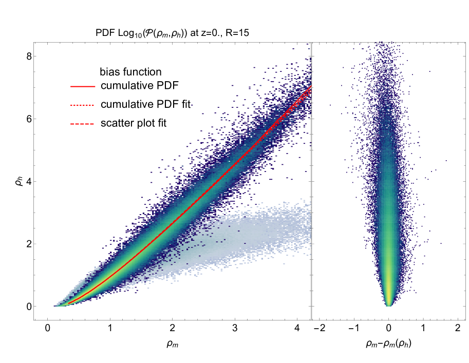
Following the observations made in Jee et al. (2012) (Jee12 hereafter), let us consider a halo density with mass-weighting (instead of number-weighting) because this makes the bias relation much tighter and considerably reduces the scatter which is illustrated in Figure 1. This observation can be understood by the intuition that mass-weighted halo densities resemble the overall dark matter density much more closely than halo number does. Note however that the mass-weighted densities of subhaloes are expected to be very similar to the mass weighted density of haloes (with no substructure) as the mass is almost preserved from haloes to subhaloes. This paper considers subhaloes as defined in Section 3.1 because they can be related to galaxies using abundance matching (Kravtsov et al., 2004; Vale & Ostriker, 2004), see Section 3.2.4.
3.2 Bias models: mean bias relations and their scatter
Uhlemann et al. (2016b) showed that the model for the PDF of the dark matter density field with the variance of the log-density as a driving parameter was accurate at the percent level for variances . Hence, the question of how to obtain a similarly accurate model for the PDF of the density field of a biased mass tracer boils down to successfully describing the effective bias relation between dark matter densities in spheres and the corresponding densities in spheres of their tracers. For simplicity, this bias model is formulated between dark matter and halo (or galaxy) densities for spheres of identical radii, so from now on stands for . While in general one would expect that the full joint PDF of dark matter and tracer densities is needed, including the scatter, it is shown in what follows that an accurate mean bias relation is enough to obtain an excellent model for the biased tracer PDF. This is in the spirit of large deviation statistics, that has been previously applied to argue that the mean local gravitational evolution given by spherical collapse is good enough to predict the dark matter PDF at fixed radius at percent accuracy111The large-deviation principle states that the statistics is dominated by the path that minimises the “action” – or in our case the rate function – in order to maximise the probability. This most likely path or dynamics can be decomposed into a gravitational part, given by the spherical collapse, and an astrophysical part, given by the mean bias relation..
3.2.1 Polynomial bias model in log-densities
In order to map the dark matter PDF to the halo PDF, let us rely on an ‘inverse’ bias model writing the dark matter density as a function of the halo density which, according to Jee12, has a better performance than the ‘forward’ bias model . These bias parameters characterise the inverse relation and in particular our linear bias will typically have values around signalling positive linear forward bias around 2. Again, following Jee12, let us use a quadratic model for the log-densities (rather than for the densities) which reads
| (10) |
It was checked that the higher order bias parameters are negligible, for all redshifts and radii considered here, and lead to very minor improvements of the quality of fit that do not warrant the use of this additional parameter. Note that, since the offset is additive in the log-densities, it ensures a multiplicative renormalisation for the density222When expanding the quadratic bias model for log-densities in the halo density contrast one obtains Interestingly, for the similar radii , Mpc one finds identical and while and differ., which is preferable according to an analytical result of Frusciante & Sheth (2012) that has been obtained from a lognormal mapping. Jee12 emphasize that the reason why equation (10) can be approximated by a linear bias model for the density fluctuations on large scales is that the ranges of log-densities and become small and not because the bias relation itself becomes linear. This is particular relevant here when focussing on the tails of the distribution of densities and hence the regime where linear bias is not sufficient.
| param | variance | correlation | bias | |||||
|---|---|---|---|---|---|---|---|---|
| 0 | 10 | 0.613 | 1.276 | 0.041 | 0.093 | 0.068 | 0.604 | 0.058 |
| 0 | 15 | 0.475 | 0.855 | 0.043 | 0.099 | 0.036 | 0.618 | 0.058 |
| 1 | 10 | 0.411 | 1.006 | 0.015 | 0.067 | 0.054 | 0.460 | 0.055 |
| 1 | 15 | 0.310 | 0.692 | 0.016 | 0.071 | 0.028 | 0.473 | 0.055 |
| 0 | 10 | 0.614 | 1.286 | 0.041 | 0.115 | 0.086 | 0.566 | 0.052 |
| 0 | 15 | 0.476 | 0.911 | 0.043 | 0.122 | 0.048 | 0.574 | 0.052 |
3.2.2 Parametrisation-independent inference of bias
Following the idea of Sigad et al. (2000); Szapudi & Pan (2004), a direct way to obtain the mean bias relation is to use the properties of the cumulative distribution functions (CDFs), defined as , so that
| (11) |
This parametrisation-independent bias extraction is used to verify the accuracy of the polynomial log-bias model, equation (10), as described below.
3.2.3 Density scatter plots from numerical simulation
Figure 1 presents a scatter plot showing as a function of for redshift and radius Mpc in order to assess how well bias models characterise the halo density bias. The lines correspond to the mean bias obtained in a parametrisation-independent way from the CDF method (red line) and fits based on a quadratic bias model for the log-densities (dotted and dashed red line) according to equation (10). The corresponding values of the best-fit bias parameters are given in Table 1 for different redshifts and radii. The second-order bias model for the logarithmic densities based on equation (10) agrees almost perfectly with the parametrisation-independent way of inferring bias using CDFs as in equation (11) and matches simulation results very well, as has been observed in Jee12 for a wide range of mass cuts, smoothing lengths, and redshifts. Indeed, differences in the fits are almost imperceptible to the eye and at the sub-percent level throughout, except for the extreme low and high-density tail, and the residual scatter around the mean polynomial log-bias model is very symmetric and uniform. This has to be contrasted with a quadratic model in the mass-weighted halo densities that can be shown to have a clear residual skewness and to be significantly less accurate (residuals of about 2% between , increasing more steeply in the tails). Since the mean bias relation is used to map the PDFs, having an even scatter around the mean relation is advantageous to mitigate possible effects of the scatter. Hence in the following the polynomial bias model for the log-densities will be used.
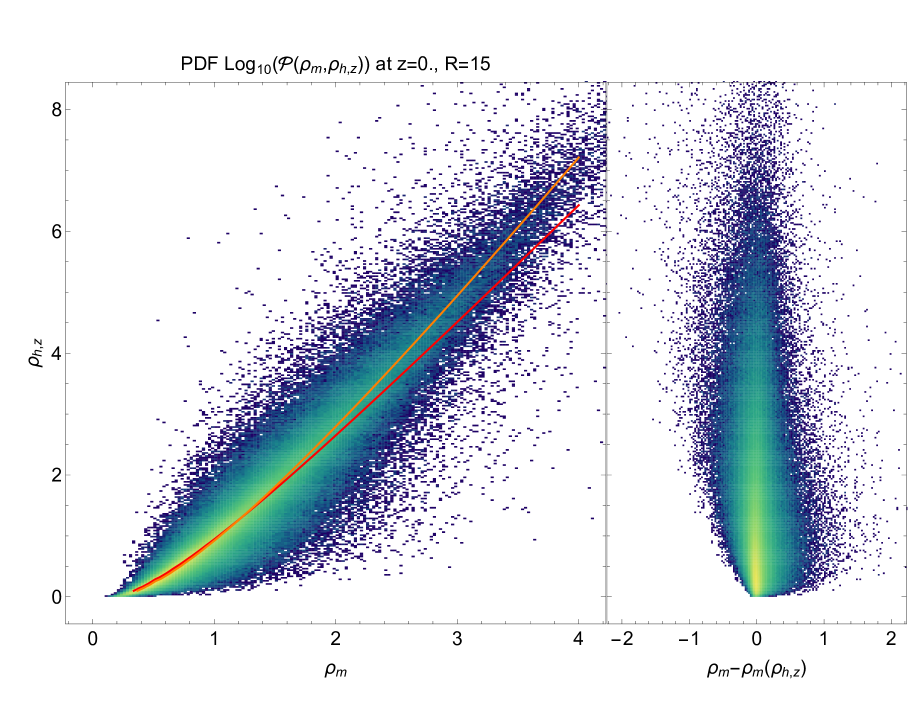
Furthermore, Figure 2 presents a scatter plot for the halo density determined in redshift space . As was done in real space, a parametrisation-independent extraction of the mean bias relation was used as a complement to the polynomial bias model in the log-densities (10) for mass-weighted halo densities in redshift space, thereby extending the results of Jee12. When comparing the scatter plot from redshift space to its real space analogue (shown in Figure 1), one can clearly see a enhanced scatter around the mean bias relation. Yet, this extra scatter does not directly translate into inaccuracies of the PDF, as shown in Figure 5.
3.2.4 Applicability to galaxies
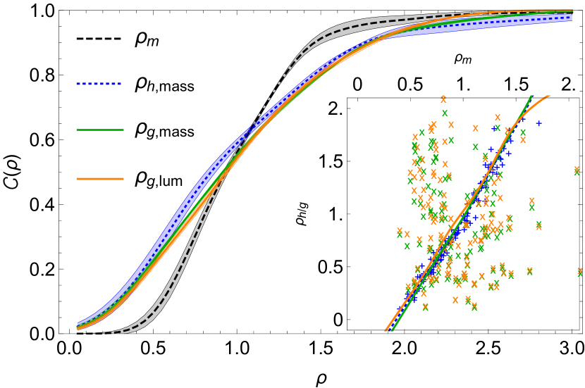
In order to check to which extent our formalism developed for haloes will be applicable to galaxies, mass-weighted densities of haloes, galaxies and luminosity-weighted densities of galaxies were extracted from the state-of-the-art Horizon-AGN simulation, a full-physics hydrodynamical simulation in a cosmological volume (Dubois et al., 2014a). Dark matter and mass-weighted subhalo densities in 125 non-overlapping spheres of radius Mpc are extracted from the simulated box at . In order to mimic observational measurements, mass- and luminosity-weighted (in the -band) galaxy densities are extracted from the simulated lightcone in a redshift range around . Realistic galaxy luminosities have been computed in post-processing using spectral synthesis, and galaxy stellar masses have been computed from photometry using SED-fitting, as usually done in observational datasets, which naturally allows to incorporate realistic errors (Laigle et al. in prep, see Appendix C for more details). We didn’t find any qualitative difference between the mean bias relations for galaxies and haloes. Indeed, Figure 3 displays the CDF of dark matter, mass-weighted subhaloes as well as mass- and luminosity-weighted galaxies together with the corresponding scatter plot. The blue, green and orange lines and points correspond to resp. mass-weighted subhaloes, galaxies and luminosity-weighted galaxies and are practically undistinguishable given the statistics we have333Note that, even for this state-of-the-art galaxy simulation, the box size is too small and hence the number of spheres not large enough to compare the PDFs directly., although the scatter of the galaxies is significantly increased compared to halos. This is a very promising result that motivates the use of mass-weighted halo density fields in this work. A thorough study of galaxy and halo bias in Horizon-AGN will be the topic of a forthcoming paper (Chisari et al, in prep.). Note that, if one weights the galaxy densities with the mass of the host subhalo, the resemblance is even closer and the scatter reduced. But in practice this would require both measuring the stellar masses (or luminosities) of the galaxies and relating them to the masses of the host subhaloes. The accuracy of the former is limited by the error on galaxy mass which is expected to be a function of the mass and redshift. At low redshift (), the observed galaxy mass is generally underestimated compared to the intrinsic one and in general one can have a discrepancy up to depending on the quality of the spectroscopy or photometry available to estimate the stellar mass (see e.g. Pforr et al., 2012; Mobasher et al., 2015, Laigle et al. in prep). When adding a Gaussian noise of this size to the measured halo masses, as explicitly checked at for the radii Mpc, the corresponding PDFs of the mass-weighted halo densities remain almost unchanged except for their deep tails. The best-fit bias parameters change only marginally, with the linear and largest bias parameter being most robust (sub-percent difference) and larger effects on the relatively small bias-renormalisation (5-7% difference) and the quadratic bias (2-4% difference). For relating galaxy mass to halo mass, one can then use techniques based on subhalo abundance matching (SHAM, Behroozi et al., 2010) or its extensions (see e.g. Yang et al., 2012; Kulier & Ostriker, 2015), which are very close in spirit to the modelling of bias used here and typically give an error of a similar size than the mass determination, at least for large halo masses. The same idea can be applied to galaxy luminosities (see e.g. Vale & Ostriker, 2004, 2006; Cooray & Milosavljević, 2005) which can be measured much more reliably than galaxy masses. Very recently, Moster et al. (2017) presented an empirical model for galaxy formation finding that average star formation and accretion rates are in good agreement with models following an abundance matching strategy. One can also determine the galaxy-halo connection, in particular the stellar-to-halo mass ratio, from a joint lensing and clustering analysis of observations (as done in Coupon et al., 2015; Zu & Mandelbaum, 2015) when using the halo occupation distribution (HOD) framework that assumes that the number of galaxies per halo is solely a function of halo mass, split into central and satellite contributions.
4 The biased tracer density PDF
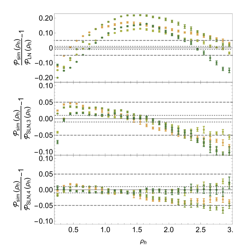
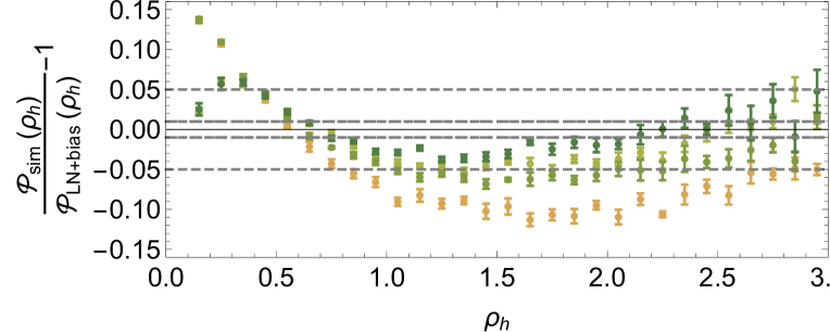
Having established the accuracy of the bias model, let us now combine it with the one-point dark matter PDF and two-point sphere bias to obtain the one-point halo PDF and two-point halo bias. The accuracy of the analytical predictions for one- and two-point statistics will be checked against the simulation. In Appendix A the analytical model for the halo PDF is compared to phenomenological reconstructions based on lognormal distributions and their extensions through cumulant expansions.
4.1 Mapping to the tracer PDF with the mean bias relation
The halo density PDF, , can be generally written as a convolution of the dark matter PDF and the conditional PDF of finding a certain halo density given a dark matter density
| (12) |
where the conditional PDF depends on the details of halo formation and its associated parameters such as, e.g., halo mass, smoothing scales, and redshift, but also includes stochasticity which results from an incomplete understanding of the formation process (e.g., Dekel & Lahav, 1999). One could attempt to model the joint PDF with the help of simulated and observed datasets in the spirit of the halo model of galaxy clustering (e.g., Cooray & Sheth, 2002; Berlind & Weinberg, 2002). Here, the scatter around the mean relation between and will be neglected: this nonetheless leads to an excellent model for the halo PDF provided the underlying bias model is appropriate. Equipped with a bias model for the mean relation , the halo PDF is now obtained from the dark matter PDF in equation (1) by conservation of probability
| (13) |
where it is assumed that is a strictly monotonic function. Using equation (6), the halo two-point PDF can eventually be written down as
| (14) |
One can then define the modulation of the two-point correlation function, the sphere bias for halos from the result for dark matter given in equation (8)
| (15) |
where the ratio of correlation functions is given by
| (16) |
and can be approximated by expanding the log-bias relation to first order to obtain .
4.2 Checking the accuracy of halo PDF against simulations
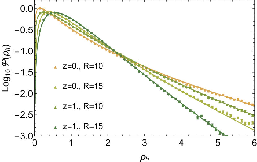
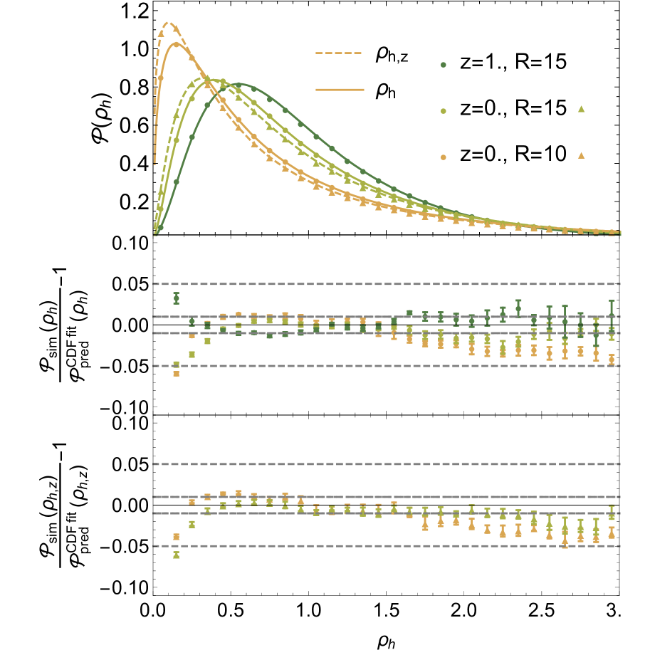
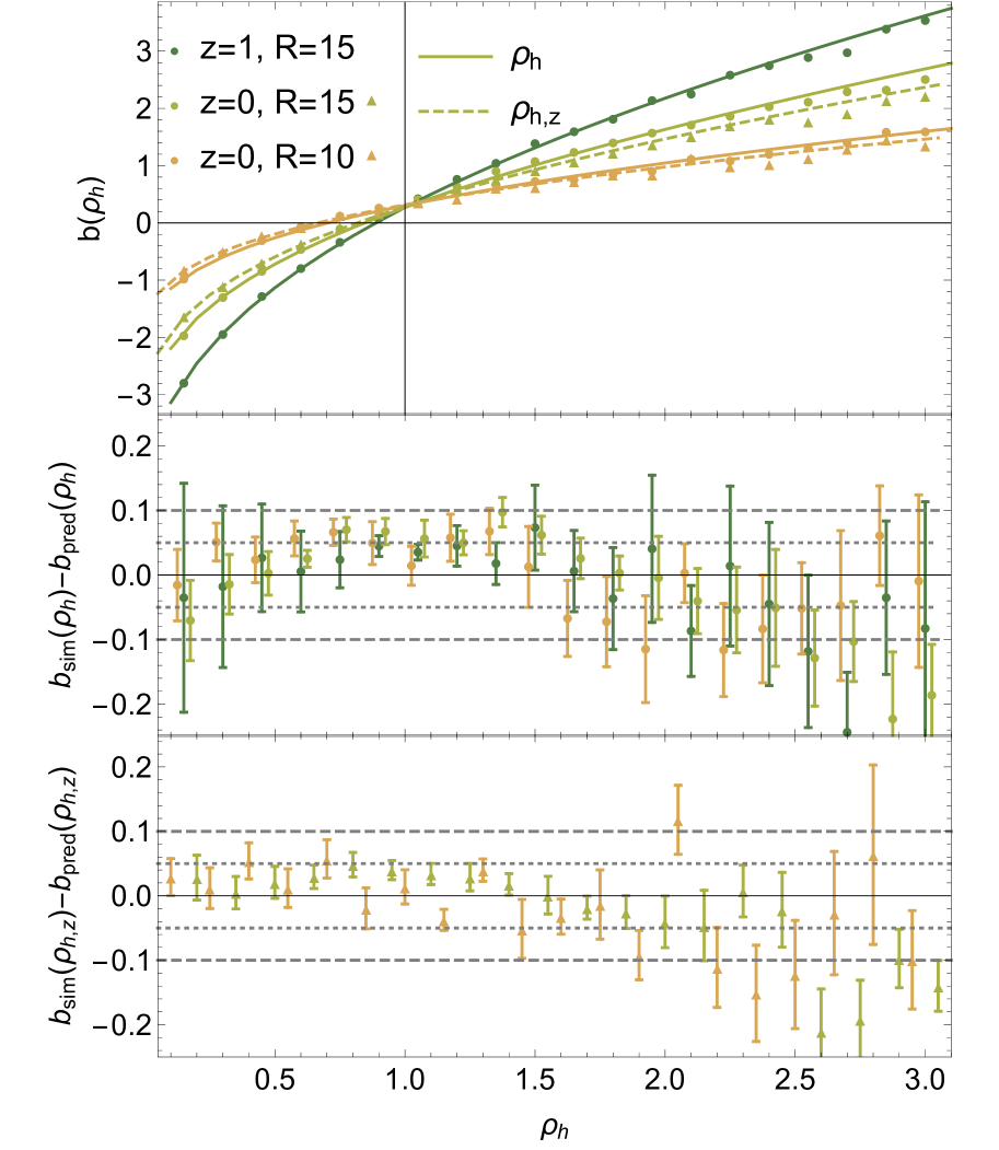
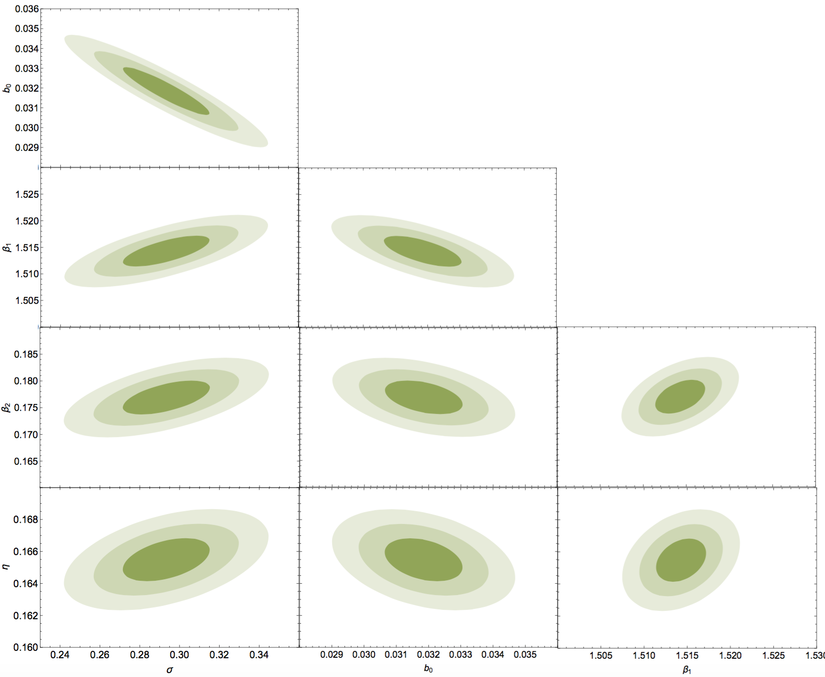
Figure 4 and 5 show the result of the halo-PDF obtained from (13) using the measured variance of the dark matter log-density and the best-fit bias parameters for the bias model for the log-densities up to second order reported in Table 1. The prediction for the halo PDF clearly matches the data, presenting residuals at the percent level in a wide range of halo densities from 0.2 to 3, in both real and redshift space. This should be contrasted to the log-normal PDF family discussed in Appendix A. This is very encouraging given the level of non-linearities involved in halo formation. The scatter of the bias relation could in principle have degraded the accuracy of the PDF, but Figure 5 shows that it turns out to be a small effect. This remains true for counts of halos in redshift space, even though the redshift space scatter plot displayed significantly larger scatter than its real space counterpart. Figure 6 compares the prediction for the sphere bias function in both real and redshift space, based on the same inputs as used for the halo PDF, with the measurements from the simulation and is also displaying excellent agreement. Note that, for the redshift-space correlation, which has an angular dependence, only the monopole is effectively probed. To measure the sphere bias function, encoding the excess correlation between densities in spheres according to equation (7), a separation of Mpc is chosen, giving a grid of non-overlapping spheres. The densities of the 6 neighbouring spheres are collected in bins of width ; precise formulas are given by equations (19) and (20) in Uhlemann et al. (2017).
5 Application: parameter estimation
One of the main goals of constructing tracer statistics is to extract cosmological parameters from counts-in-cells. Let us now make use of the one-point halo PDF (13) alone or combine it with the density-dependent sphere bias (15) to estimate either the bias parameters, the underlying dark matter variance, or both.
Due to the strong (although not complete) degeneracy between the dark matter variance and linear bias (that can be shown to hold exactly for a linearly biased lognormal PDF (see Appendix A), and is given as at leading order in perturbation theory according to equation (28)), it turns out one cannot use the one-point statistics alone to jointly determine the dark matter variance and bias parameters. This is not at all surprising, given the well-known degeneracy between linear bias and the clustering amplitude, caused by the fact that a low matter fluctuation amplitude can be masked out by a high galaxy bias or vice versa (see e.g. Seljak et al., 2005). In principle, if (i) all the statistics could be measured exactly, (ii) the truncation in the bias model was fully justified, and (iii) the dark matter PDF was exactly given by the LDS model and in particular different from log-normal, then it should be possible to measure jointly the dark matter variance and the three bias parameters. In practice, when considering limited noisy samples, only the first three cumulants (mean, variance, skewness) carry enough information in a statistical sense, so that measuring the one-point PDF can only put three constraints on the parameters of the model. For a quadratic bias model, this means that one effectively ends up with a degeneracy line (i.e a one-dimensional manifold) in the four dimensional parameter space. Indeed, subsection 5.1 shows how in practice the one-point model does not yield enough information to measure both on realistic surveys and discusses complementary strategies when relying on one-point statistics only, while subsection 5.2 explains why one- and two-points halo counts does break this degeneracy in principle. Finally subsection 5.3 shows how a joint fit of both counts from the HR4 simulation yields an estimate of all four parameters plus the dark matter correlation function.
5.1 Bias-variance degeneracy in one-point statistics
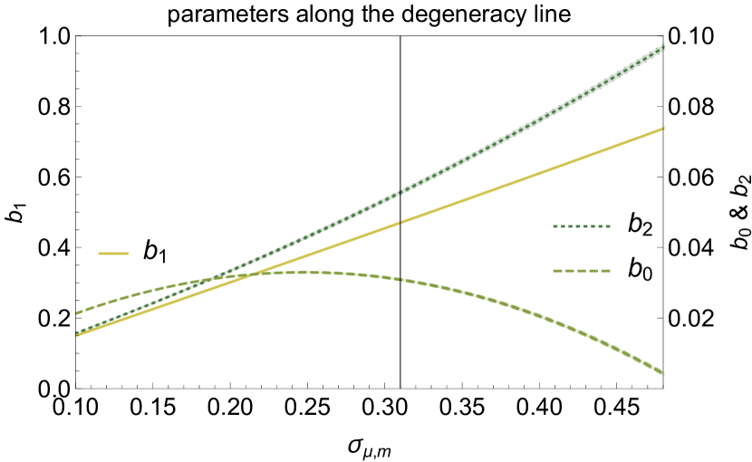
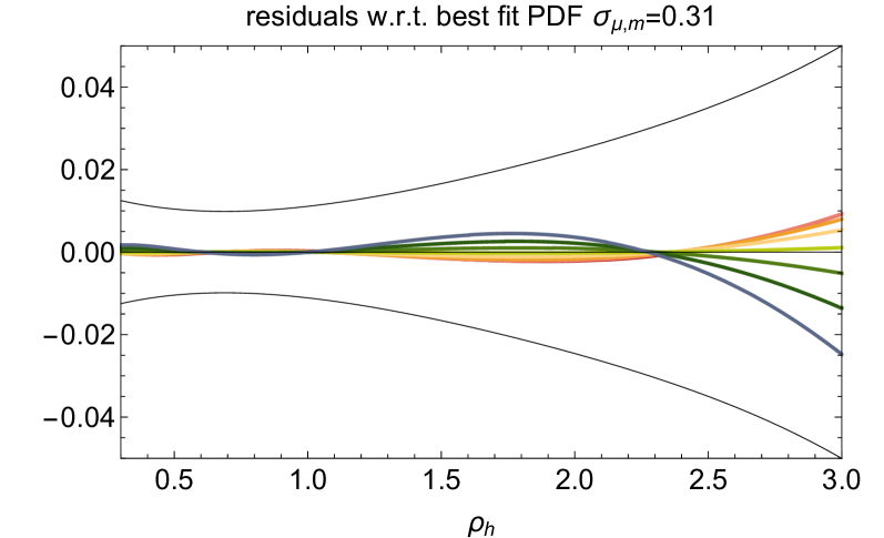
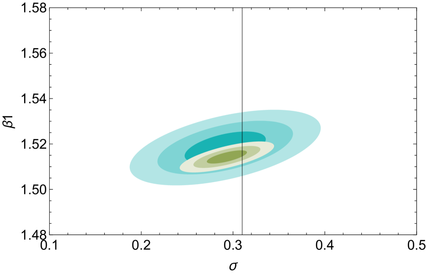
In order to quantify the bias-variance degeneracy in one-point statistics, let us measure the density PDF at in the Horizon-run 4 simulation covered by spheres of radius Mpc, and get one-sigma error bars as the error on the mean estimated from 8 subcubes. Let us describe the degeneracy with as the curvilinear coordinate and for each value of between 0.1 and 0.5, and fit the measured non-linear PDF from to with bins as this is the regime where the model is expected to work well. The one-sigma confidence intervals of the bias parameters as a function of are displayed in the top panel of Figure 7. As expected from the perturbative argument, the degeneracy line is dominated by a linear relationship between and (with slope ) with higher order correction leading to non-zero (but small) values of and . The parabolic shape of and the linear growth of with , as well as their smallness, can in fact be understood perturbatively, as shown in equations (27) and (31) in Appendix B.2. The bottom panel of Figure 7 shows that the predicted PDFs along the degeneracy line are all within the one-sigma error bars of the simulation and therefore cannot be distinguished. Combining this observable with other probes or using a model for the dark matter variance should in principle break this degeneracy.
If the nonlinear dark matter variance was known, for example from empirical relations found in simulations (such as Repp & Szapudi, 2017) or higher order perturbation theory (see e.g. Scoccimarro & Frieman, 1996), one could use the analytic dark matter PDF (1) to obtain the CDF of dark matter and then the bias relation using equation (11) by measuring the halo CDF . Note that this procedure essentially looks for a nonlinear transformation of halo-densities such that the result is distributed according to the dark matter PDF equation (1), and hence similar in spirit to the idea of Gaussianising the field (see e.g. McCullagh et al., 2016).
Conversely, if the bias parameters (including their time evolution) were known from either theory or measured from an independent probe, one could use the analytic halo PDF (13) to determine the dark matter variance and use this to constrain for example the dark energy equation of state as demonstrated for dark matter in Codis et al. (2016a). Analytical attempts to predict cumulants of the halo density have been based on bias models starting from Press-Schechter (Casas-Miranda et al., 2002, 2003), its extensions like excursion sets or peak theory, or the halo model (Fry et al., 2011). Note that, to take advantage of this idea one needs access to the bias that relates averaged halo and matter densities rather than the bias based on n-point functions. While there is a mapping between the two in the large-scale limit, for Mpc, they are not equal and their relation depends on the shape of the power spectrum as well as the smoothing radius and filter shape, as pointed out in Desjacques et al. (2016). For particular observational signatures that are not degenerate with bias, such as local primordial non-Gaussianity (Uhlemann et. al. in preparation), the present formalism allows to take the nature of tracers into account and hence to obtain more realistic constraints. In principle, future peculiar velocity surveys could also gain us qualitative insights into biasing following the idea described in Uhlemann et al. (2016a), although their statistical power is unlikely to yield accurate enough constraints.
5.2 Joint one- and two-point statistics: the basic idea
In order to break the degeneracy between bias parameters and the dark matter variance, one can make use of the two-point statistics from equation (4.1) to jointly constrain the dark matter variance and biases. The two-point halo PDF is built from the one-point halo PDFs (13) and the density-dependent sphere bias (15) that modulates the two-point correlation function which were successfully compared to numerical simulations in Section 4.
Let us present here the basic idea behind the degeneracy lift. The leading-order mixed cumulant depends on the two-point sphere bias function via
| (17) |
Since the sphere bias function is not linear , especially in the tails that are sensitive to , equation (17) differs from the one-point cumulant given by the skewness
| (18) |
The leading order expressions444Note that, at that order, the cumulants of the density and log-density only differ by a constant, see Uhlemann et al. (2016b). relating the corresponding dark matter and halo cumulants for the adopted (inverse quadratic in the log-densities) biasing model are consistently given by
| (19) | ||||
| (20) |
Combining equations (19) and (20) allows us in principle to solve for the bias parameters, by relying on theoretical predictions for the dark matter cumulants on the one hand, and measurements for the halo cumulants on the other hand555These expressions closely resemble those given in Bel & Marinoni (2012) which use a forward biasing model in the densities. This paper relies on the lowest order cumulants predicted by tree-order perturbation theory and combines them in a difference that is suspected to be more robust than the individual cumulants..
This paper extends this cumulant based strategy by taking advantage of the full two-point information (Bernardeau & Schaeffer, 1992; Munshi et al., 2000) which consistently include higher order cumulants leading to improved accuracy, as demonstrated in Codis et al. (2016a); Uhlemann et al. (2017). In effect, instead of being restricted to the lowest order cumulants, it makes simultaneous use of the one-point PDF and the two-point sphere bias function. Indeed, it can be shown that the two-point sphere bias’ slope with respect to the density is sensitive to bias alone, hence the joint analysis of both counts breaks the degeneracy. Appendix B sketches a proof at the perturbative level.
5.3 Joint one- and two-point statistics: a worked example
Let us finally present a worked out fiducial experiment that allows to simultaneously obtain the dark matter variance, correlation function as well as the bias parameters from measurements of one-point halo PDF given a redshift and sphere radius and the two-point halo sphere bias at a separation . In practice, sampling the joint likelihood for 5 parameters is computationally expensive and tricky because the joint PDF is noisy and the signal coming from the sphere bias rather small666Note also that the tracer PDF’s boundaries depend on the bias parameters, which, combined with the fact that the LDS model is only accurate on a finite range of densities adds an extra layer of complexity to the likelihood exploration.. Let us therefore resort here to a simpler fitting procedure to illustrate the capability of the one- and two-point halo statistics for jointly constraining the dark matter variance and correlation along with the bias parameters. A data sample is derived from the simulation by binning the halo densities and measuring a histogram for the PDF in the range with bin width and the scaled halo sphere bias
| (21) |
in the range with bin width . The scaled halo sphere bias is used instead of the halo sphere bias as this is the direct observable. The LDS prediction is given by
| (22) |
where the prefactor encodes the difference of the correlation function and is tabulated using a 5th order Taylor expansion of near one.
Using this sample, a nonlinear model fit is implemented for the two functions and with weights determined by the errors from the measured PDF and bias function (using bootstrapping over 8 subsamples of the simulation). The result of the fit for the parameters and the associated uncertainties is given in Table 2 (see also Figure 8 for the corresponding figures of merit) and agrees very well with the directly measured values reported in Table 1. In particular, the sphere bias (i.e the two-point statistics of density in spheres) is shown as anticipated to break the degeneracy. Since the dark matter correlation function enters as an overall amplitude, the degeneracy is broken by the information contained in the shape of the sphere bias function, rather than its amplitude, as can be seen perturbatively in Appendix B. As the noise is more important in the two-point sphere bias than in the one-point density PDF, the error budget on the parameters of the model is dominated by the accuracy on the measurement of .
The total number of spheres () is of the order of the number of spheres that a survey like Euclid will probe at a redshift around (Codis et al., 2016a). Hence one can expect this novel idea to be applicable to real data in a very near future, which will allow us to measure consistently the growth of fluctuations across cosmic time (through the dark matter variance ) and to characterise galaxy biasing (through a set of bias parameters at different redshifts). The accuracy of the constraints on those parameters depends on the accessible survey volume and therefore the number of spheres , in a way which can be studied by subsampling the simulation. Redoing the above-described analysis on 8 subcubes of the simulation, yields the average best fit values (notably 0.29, 0.030, 1.518, 0.181, 0.161 for , , , , ) are consistent with the parameters estimated from the full box (0.29, 0.032, 1.514, 0.177, 0.165), as seen on Figure 9. The mean standard deviation are respectively 0.033, 0.0030, 0.0052, 0.0056, 0.0023 (to be compared with the one-sigma error bars from the full volume: 0.016, 0.00089, 0.0021, 0.0023, 0.00099), which is consistent with a scaling. Overall, the typical one-sigma errors evolve as and .
The above presented experiment is of course fairly idealized at various levels. It may turn out to be too optimistic, but should nonetheless provide a framework in which to implement a dark energy experiment based on count-in-cells.
| param | dark matter | tracer bias | ||||
|---|---|---|---|---|---|---|
| 1 | 15 | |||||
6 Conclusions
Starting from a very accurate model for the dark matter density-in-cells, we extended it to biased tracers such as dark haloes or galaxies and compared them to the state-of-the-art Nbody simulation Horizon Run 4 in real and redshift space. Our main findings can be summarised as follows:
-
1.
on scales of the order of 10 Mpc, mass-weighted subhalo densities show considerably less scatter than their number-weighted version; they can be accurately fit with a quadratic bias model in the log-densities and closely resemble the bias relation of mass-weighted galaxy densities.
-
2.
Using a quadratic mean bias model for log-densities and neglecting the scatter is sufficient to obtain a one-point halo PDF and two-point sphere bias that are as accurate as the underlying dark matter results when compared against simulations, see Figures 5 and 6. Combining the quadratic bias model with fitted coefficients with the dark matter PDF from large deviation statistics with the measured dark matter variance, the accuracy of the halo PDF is well within 5% over a wide range of densities, in both real and redshift space.
-
3.
The one-point PDF yields access to a one dimensional manifold in the four dimensional parameter space of dark matter variance and quadratic bias.
-
4.
Combining the one-point halo PDF and the two-point halo sphere bias, one can jointly constrain the nonlinear dark matter variance and correlation as well as the bias parameters, and hence disentangle tracer bias from nonlinear gravitational evolution. This is of interest both from the point of view of dark energy and non-linear power spectra estimation. The density-dependent clustering signal encoded in the two-point sphere bias is related to the concept of ‘sliced’ or ‘marked’ correlation functions (see e.g. Sheth, 2005; White & Padmanabhan, 2009; Neyrinck et al., 2016) which hence might contain valuable information about bias and could be used to break the degeneracy between linear bias and the clustering amplitude in the two-point correlation.
-
5.
Comparison to counts extracted from ‘full-physics’ hydrodynamical simulations suggest that our findings will scale from dark halos to galaxies.
The excellent accuracy of the analytical prediction for the dark matter PDF and two-point bias plays a critical role in disentangling the dark matter variance from biasing when applied to tracers. Hence, this formalism should be applied to constrain cosmology using counts-in-cells statistics in ongoing or upcoming surveys like DES, Euclid, WFIRST, LSST, KiDs, following the fiducial dark energy experiment presented in Codis et al. (2016a).
Acknowledgements
This work is partially supported by the grants ANR-12-BS05-0002 and ANR-13-BS05-0005 of the French Agence Nationale de la Recherche. CU is supported by the Delta-ITP consortium, a program of the Netherlands organisation for scientific research (NWO) funded by the Dutch Ministry of Education, Culture and Science (OCW). We thank Tobias Baldauf, Karim Benabed, Donghui Jeong, Marcello Musso, Fabian Schmidt, Ravi Sheth and the participants of the workshops ‘Statistics of Extrema in Large Scale Structure’ and the ‘Biased Tracers of Large-Scale Structure’ for discussions. We thank Iary Davidzon for having run the SED-fitting on the photometry of the simulated galaxies in the Horizon-AGN simulation in order to compute mock observed stellar masses. CU thanks IAP and CITA, while MF, DP and SC also thank KIAS for hospitality while some of this work was done. Many thanks to Stéphane Rouberol for smoothly running the Horizon cluster which is hosted by the Institut d’Astrophysique de Paris, and to our colleagues who produced and post processed the Horizon-AGN/ HR4 simulations.
References
- Abell (1958) Abell G. O., 1958, ApJS, 3, 211
- Adelberger et al. (1998) Adelberger K. L., Steidel C. C., Giavalisco M., Dickinson M., Pettini M., Kellogg M., 1998, ApJ, 505, 18
- Arnouts et al. (2002) Arnouts S., et al., 2002, MNRAS, 329, 355
- Aubert et al. (2004) Aubert D., Pichon C., Colombi S., 2004, MNRAS, 352, 376
- Bahcall & Soneira (1983) Bahcall N. A., Soneira R. M., 1983, ApJ, 270, 20
- Baldauf et al. (2011) Baldauf T., Seljak U., Senatore L., Zaldarriaga M., 2011, J. Cosmology Astropart. Phys., 10, 031
- Balian & Schaeffer (1989) Balian R., Schaeffer R., 1989, A&A, 220, 1
- Bardeen et al. (1986) Bardeen J. M., Bond J. R., Kaiser N., Szalay A. S., 1986, ApJ, 304, 15
- Baugh (2006) Baugh C. M., 2006, Reports on Progress in Physics, 69, 3101
- Behroozi et al. (2010) Behroozi P. S., Conroy C., Wechsler R. H., 2010, ApJ, 717, 379
- Bel & Marinoni (2012) Bel J., Marinoni C., 2012, MNRAS, 424, 971
- Bel et al. (2016) Bel J., Branchini E., Di Porto C., Cucciati O., Granett B. R., Iovino A., et al. 2016, A&A, 588, A51
- Berlind & Weinberg (2002) Berlind A. A., Weinberg D. H., 2002, ApJ, 575, 587
- Bernardeau (1992) Bernardeau F., 1992, ApJ, 392, 1
- Bernardeau (1994a) Bernardeau F., 1994a, A&A, 291, 697
- Bernardeau (1994b) Bernardeau F., 1994b, ApJ, 427, 51
- Bernardeau & Kofman (1995) Bernardeau F., Kofman L., 1995, ApJ, 443, 479
- Bernardeau & Reimberg (2016) Bernardeau F., Reimberg P., 2016, Phys. Rev. D, 94, 063520
- Bernardeau & Schaeffer (1992) Bernardeau F., Schaeffer R., 1992, A&A, 255, 1
- Bernardeau et al. (2014) Bernardeau F., Pichon C., Codis S., 2014, Phys. Rev. D, 90, 103519
- Bernardeau et al. (2015) Bernardeau F., Codis S., Pichon C., 2015, MNRAS, 449, L105
- Blanton et al. (1999) Blanton M., Cen R., Ostriker J. P., Strauss M. A., 1999, ApJ, 522, 590
- Bond et al. (1991) Bond J. R., Cole S., Efstathiou G., Kaiser N., 1991, ApJ, 379, 440
- Casas-Miranda et al. (2002) Casas-Miranda R., Mo H. J., Sheth R. K., Boerner G., 2002, MNRAS, 333, 730
- Casas-Miranda et al. (2003) Casas-Miranda R., Mo H. J., Boerner G., 2003, MNRAS, 339, 872
- Cen & Ostriker (1992) Cen R., Ostriker J., 1992, ApJ, 393, 22
- Clerkin et al. (2017) Clerkin L., et al., 2017, MNRAS, 466, 1444
- Codis et al. (2016a) Codis S., Pichon C., Bernardeau F., Uhlemann C., Prunet S., 2016a, MNRAS, 460, 1549
- Codis et al. (2016b) Codis S., Bernardeau F., Pichon C., 2016b, MNRAS, 460, 1598
- Coles (1986) Coles P., 1986, MNRAS, 222, 9P
- Coles & Jones (1991) Coles P., Jones B., 1991, MNRAS, 248, 1
- Colombi (1994) Colombi S., 1994, ApJ, 435, 536
- Cooray & Milosavljević (2005) Cooray A., Milosavljević M., 2005, ApJ, 627, L89
- Cooray & Sheth (2002) Cooray A., Sheth R., 2002, Phys. Rep., 372, 1
- Coupon et al. (2015) Coupon J., et al., 2015, MNRAS, 449, 1352
- Dekel & Lahav (1999) Dekel A., Lahav O., 1999, ApJ, 520, 24
- Desjacques et al. (2016) Desjacques V., Jeong D., Schmidt F., 2016, preprint, (arXiv:1611.09787)
- Dressler (1980) Dressler A., 1980, ApJ, 236, 351
- Dubinski et al. (2004) Dubinski J., Kim J., Park C., Humble R., 2004, New Astron., 9, 111
- Dubois et al. (2012) Dubois Y., Devriendt J., Slyz A., Teyssier R., 2012, MNRAS, 420, 2662
- Dubois et al. (2014a) Dubois Y., et al., 2014a, MNRAS, 444, 1453
- Dubois et al. (2014b) Dubois Y., Pichon C., Welker C., et al. 2014b, MNRAS, 444, 1453
- Dwek (1998) Dwek E., 1998, ApJ, 501, 643
- Fosalba & Gaztanaga (1998) Fosalba P., Gaztanaga E., 1998, MNRAS, 301, 503
- Frusciante & Sheth (2012) Frusciante N., Sheth R. K., 2012, J. Cosmology Astropart. Phys., 11, 016
- Fry (1985) Fry J. N., 1985, ApJ, 289, 10
- Fry & Gaztanaga (1993) Fry J. N., Gaztanaga E., 1993, ApJ, 413, 447
- Fry et al. (2011) Fry J. N., Colombi S., Fosalba P., Balaraman A., Szapudi I., Teyssier R., 2011, MNRAS, 415, 153
- Gaztañaga et al. (2000) Gaztañaga E., Fosalba P., Elizalde E., 2000, ApJ, 539, 522
- Haardt & Madau (1996) Haardt F., Madau P., 1996, ApJ, 461, 20
- Hurtado-Gil et al. (2017) Hurtado-Gil L., Martínez V. J., Arnalte-Mur P., Pons-Bordería M. J., Pareja-Flores C., Paredes S., 2017, preprint, (arXiv:1703.01087)
- Ilbert et al. (2006) Ilbert O., et al., 2006, A&A, 457, 841
- Jee et al. (2012) Jee I., Park C., Kim J., Choi Y.-Y., Kim S. S., 2012, ApJ, 753, 11
- Jonsson (2006) Jonsson P., 2006, MNRAS, 372, 2
- Juszkiewicz et al. (1993) Juszkiewicz R., Bouchet F. R., Colombi S., 1993, ApJ, 412, L9
- Juszkiewicz et al. (1995) Juszkiewicz R., Weinberg D. H., Amsterdamski P., Chodorowski M., Bouchet F., 1995, ApJ, 442, 39
- Kaiser (1984) Kaiser N., 1984, ApJ, 284, L9
- Kauffmann et al. (1997) Kauffmann G., Nusser A., Steinmetz M., 1997, MNRAS, 286, 795
- Kauffmann et al. (1999) Kauffmann G., Colberg J. M., Diaferio A., White S. D. M., 1999, MNRAS, 303, 188
- Kaviraj et al. (2017) Kaviraj S., et al., 2017, MNRAS, 467, 4739
- Kim & Park (2006) Kim J., Park C., 2006, ApJ, 639, 600
- Kim et al. (2015) Kim J., Park C., L’Huillier B., Hong S. E., 2015, J. Korean Astron. Soc., 48, 213
- Komatsu (2011) Komatsu E. et al ., 2011, ApJS, 192, 18
- Kravtsov et al. (2004) Kravtsov A. V., Berlind A. A., Wechsler R. H., Klypin A. A., Gottlöber S., Allgood B., Primack J. R., 2004, ApJ, 609, 35
- Kulier & Ostriker (2015) Kulier A., Ostriker J. P., 2015, MNRAS, 452, 4013
- L’Huillier et al. (2014) L’Huillier B., Park C., Kim J., 2014, New Astron., 30, 79
- Laigle et al. (2016) Laigle C., et al., 2016, preprint, (arXiv:1604.02350)
- Matsubara (2011) Matsubara T., 2011, Phys. Rev. D, 83, 083518
- McCullagh et al. (2016) McCullagh N., Neyrinck M., Norberg P., Cole S., 2016, MNRAS, 457, 3652
- Mo & White (1996) Mo H. J., White S. D. M., 1996, MNRAS, 282, 347
- Mo et al. (2010) Mo H., van den Bosch F. C., White S., 2010, Galaxy Formation and Evolution
- Mobasher et al. (2015) Mobasher B., et al., 2015, ApJ, 808, 101
- Moster et al. (2017) Moster B. P., Naab T., White S. D. M., 2017, preprint, (arXiv:1705.05373)
- Munshi et al. (1994) Munshi D., Sahni V., Starobinsky A. A., 1994, ApJ, 436, 517
- Munshi et al. (2000) Munshi D., Melott A. L., Coles P., 2000, MNRAS, 311, 149
- Neyrinck et al. (2016) Neyrinck M. C., Szapudi I., McCullagh N., Szalay A., Falck B., Wang J., 2016, preprint, (arXiv:1610.06215)
- Ohta et al. (2003) Ohta Y., Kayo I., Taruya A., 2003, ApJ, 589, 1
- Pforr et al. (2012) Pforr J., Maraston C., Tonini C., 2012, MNRAS, 422, 3285
- Pichon et al. (2010) Pichon C., Thiébaut E., Prunet S., Benabed K., Colombi S., Sousbie T., Teyssier R., 2010, MNRAS, 401, 705
- Porto (2016) Porto R. A., 2016, Phys. Rep., 633, 1
- Repp & Szapudi (2017) Repp A., Szapudi I., 2017, MNRAS, 464, L21
- Schmidt et al. (2013) Schmidt F., Jeong D., Desjacques V., 2013, Phys. Rev. D, 88, 023515
- Scoccimarro (2000) Scoccimarro R., 2000, ApJ, 542, 1
- Scoccimarro & Frieman (1996) Scoccimarro R., Frieman J., 1996, ApJS, 105, 37
- Seljak et al. (2005) Seljak U., et al., 2005, Phys. Rev. D, 71, 043511
- Senatore (2015) Senatore L., 2015, J. Cosmology Astropart. Phys., 11, 007
- Sheth (2005) Sheth R. K., 2005, MNRAS, 364, 796
- Sheth & Tormen (1999) Sheth R. K., Tormen G., 1999, MNRAS, 308, 119
- Sheth et al. (1994) Sheth R. K., Mo H. J., Saslaw W. C., 1994, ApJ, 427, 562
- Shin et al. (2017) Shin J., Kim J., Pichon C., Jeong D., Park C., 2017, preprint, (arXiv:1705.06863)
- Sigad et al. (2000) Sigad Y., Branchini E., Dekel A., 2000, ApJ, 540, 62
- Somerville et al. (2000) Somerville R. S., Lemson G., Kolatt T. S., Dekel A., 2000, MNRAS, 316, 479
- Szapudi & Pan (2004) Szapudi I., Pan J., 2004, ApJ, 602, 26
- Szapudi et al. (1996) Szapudi I., Meiksin A., Nichol R. C., 1996, ApJ, 473, 15
- Teyssier (2002) Teyssier R., 2002, A&A, 385, 337
- Uhlemann et al. (2016a) Uhlemann C., Codis S., Hahn O., Pichon C., Bernardeau F., 2016a, preprint, (arXiv:1612.00019)
- Uhlemann et al. (2016b) Uhlemann C., Codis S., Pichon C., Bernardeau F., Reimberg P., 2016b, MNRAS, 460, 1529
- Uhlemann et al. (2017) Uhlemann C., Codis S., Kim J., Pichon C., Bernardeau F., Pogosyan D., Park C., L’Huillier B., 2017, MNRAS, 466, 2067
- Valageas (2002a) Valageas P., 2002a, A&A, 382, 412
- Valageas (2002b) Valageas P., 2002b, A&A, 382, 450
- Vale & Ostriker (2004) Vale A., Ostriker J. P., 2004, MNRAS, 353, 189
- Vale & Ostriker (2006) Vale A., Ostriker J. P., 2006, MNRAS, 371, 1173
- White & Padmanabhan (2009) White M., Padmanabhan N., 2009, MNRAS, 395, 2381
- Wolk et al. (2013) Wolk M., McCracken H. J., Colombi S., Fry J. N., Kilbinger M., Hudelot P., Mellier Y., Ilbert O., 2013, MNRAS, 435, 2
- Yang & Saslaw (2011) Yang A., Saslaw W. C., 2011, ApJ, 729, 123
- Yang et al. (2012) Yang X., Mo H. J., van den Bosch F. C., Zhang Y., Han J., 2012, ApJ, 752, 41
- Zu & Mandelbaum (2015) Zu Y., Mandelbaum R., 2015, MNRAS, 454, 1161
Appendix A Lognormal reconstruction
Let us compare the LDS approach to the well-known lognormal models. The lognormal PDF, proposed first from a dynamical model for dark matter in Coles & Jones (1991) but nowadays being used as a phenomenological parametrisation for PDFs of dark matter and its tracers, has the following form
| (23) |
where the variance of the log-density can be treated as free parameter and the mean of the log-density is connected to the variance via by requiring a unit mean density . The skewed lognormal PDF as introduced in Colombi (1994), involves an Edgeworth expansion around the lognormal PDF and reads
| (24) | ||||
with the normalised log-density , its rescaled cumulants and the probabilist’s Hermite polynomials 777Note that Edgeworth expansions are known to be problematic in the tails of the distribution because the expression in the brackets can eventually become negative depending on the size of the corrections in the cumulant expansion.. A comparison between the accuracy of the three different lognormal based models, when the underlying parameters (the mean , variance , skewness and kurtosis of the log-density) are measured from the simulated halo densities is shown in Figure 10. The generalized normal distribution adopted by Shin et al. (2017) to fit dark matter PDFs has very similar properties to the skewed lognormal PDF in the range of radii we consider and hence will not be discussed here.
The lognormal dark matter PDF can be combined with a polynomial bias model for the log-densities. For a linear bias model of the log-densities, the resulting halo PDF is again lognormal with variance and mean given by and , once the dark matter mean density is fixed to one so that . In addition, the halo mean density being one, one gets an additional contraint which relates the constant bias shift to the linear bias factor and the variance according to and agrees with the leading order perturbative result. In this model, there is a full degeneracy between the linear bias and the log-variance of the underlying dark matter .
Let us now consider a quadratic log-bias model. Even if the dark matter PDF was close to lognormal (which is typically the case at accuracy, see Uhlemann et al., 2017), this nonlinear mapping induces extra terms in the exponential. If one expands these terms in an Edgeworth-like fashion, one can see that nonlinear bias naturally feeds into higher order cumulants, in particular the skewness and kurtosis, which is why it is necessary to go to the skewed lognormal forms to fit the measured halo PDF. The residuals obtained when augmenting the lognormal dark matter PDF with the quadratic bias model with measured parameters are shown as comparison in the lower panel of Figure 10. In this case, the predicted PDF is slightly less accurate than the large-deviation prediction, with two additional parameters that cannot easily be related to bias because they mix in contributions from the dark matter PDF, which is significantly better fitted by a skewed lognormal. This is in contrast with the LDS formalism that clearly disentangles the effect of gravitational evolution (parametrised through the nonlinear dark matter variance) from nonlinear biasing (parametrised through the bias parameters).
Appendix B Breaking degeneracies
The main text has shown that with a practical implementation of the LDS formalism, one can accurately measure bias parameters and dark matter variance, and break the degeneracies by including information from two-point statistics, an idea also followed by Bel & Marinoni (2012) in another context. Let us illustrate these findings using perturbation theory.
B.1 One-point PDF
From equation (10), one can easily compute the relation between halo and matter contrast within the quadratic log bias model
| (25) |
Expanding this relation for small contrasts yields perturbative bias consistency relations. First, imposing a zero mean for the halo contrast allows to get at all orders in the dark matter variance
| (26) |
with
| (27) |
The measured halo variance then imposes a relation between the dark matter variance and the bias parameters which reads
| (28) |
with
| (29) |
The constraints are therefore dominated by this degeneracy between and at first order in PT. After the mean and the variance, the PDF will typically pick up the information from the skewness. Let us therefore compute perturbatively the skewness of the halo density field. At first order, it reads
| (30) |
This latter equation gives a relation between and at first order
| (31) |
Equations (28) and (31) predict a linear degeneracy between on the one hand and and on the other hand and which is indeed observed when performing the model fitting (see Figure 7). This model fitting described in Section 5 eventually gathers all the information coming from the mean, variance, skewness and higher order cumulants in a fully consistent way (because LPD provides the PDF and therefore the full statistics). In principle the knowledge of the full hierarchy of cumulants eventually break those degeneracies if the LDS model if exact. In practice, i) sample noise prevents accurate measurements of the higher order cumulants (kurtosis etc) which scale like higher power of the variance ( and above); ii) loop corrections in the skewness that are not accounted for in the LDS model appears at the same perturbative order as those higher order cumulants and therefore do not allow us to fully break the degeneracy between the parameters. To break this degeneracy, one must involve two-point statistics as described in the next section.
B.2 Two-point PDF
Let us assume that the two-point PDF of the matter density is well described by its large-scale approximation given by equation (6). The sphere bias can be exactly computed using the large-deviation principle (Codis et al., 2016b; Uhlemann et al., 2017). A fair approximation for small densities is given by
| (32) |
Remarkably, plugging in the bias relation in , shows that the sphere bias of the halo density field behave at small density as
| (33) |
where
and . Obviously, the overall amplitude in cannot be measured because it is degenerate with the unknown dark matter correlation function but the ratio between the slope called and intercept can
| (34) |
This ratio is in particular proportional to and does not depend on the variance. Constraining this ratio, as is done in the joint fit presented in the main text will therefore break the degeneracy in equation (28).
Appendix C The Horizon-AGN simulation
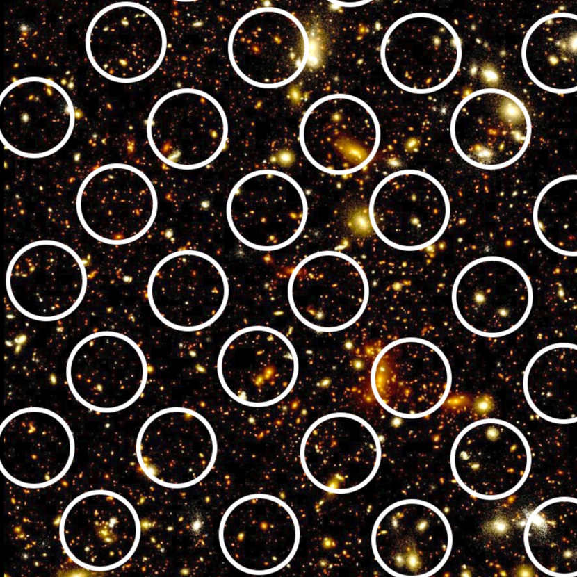
Let us briefly describe the cosmological hydrodynamical simulation used in the main text, horizon-AGN (Dubois et al., 2014b). The simulation http://www.horizon-simulation.org/ is run with a CDM cosmology with total matter density , dark energy density , amplitude of the matter power spectrum , baryon density , Hubble constant , and compatible with the WMAP-7 data (Komatsu, 2011). The size of the simulation box is on a side, and the volume contains DM particles, corresponding to a DM mass resolution of . The simulation is run with the ramses code (Teyssier, 2002), and the initially coarse grid is adaptively refined down to proper kpc, with refinement triggered in a quasi-Lagrangian manner: if the number of DM particles becomes greater than 8, or the total baryonic mass reaches 8 times the initial DM mass resolution in a cell. It lead to a typical number of gas resolution elements (leaf cells) in the simulation at . Heating of the gas from a uniform UV background takes place after redshift following Haardt & Madau (1996).
Star formation occurs in regions of gas number density above following a Schmidt law: , where is the star formation rate mass density, the gas mass density, the constant star formation efficiency, and the local free-fall time of the gas. Feedback from stellar winds, supernovae type Ia and type II are included into the simulation with mass, energy and metal release. The simulation also follow the formation of black holes (BHs), which can grow by gas accretion at a Bondi-capped-at-Eddington rate and coalesce when they form a tight enough binary. BHs release energy in a quasar/radio (heating/jet) mode when the accretion rate is respectively above and below one per cent of Eddington, with efficiencies tuned to match the BH-galaxy scaling relations at (see Dubois et al., 2012, for details). A lightcone has been generated from the simulation, as described in Pichon et al. (2010). The area of the lightcone is 5 deg2 below , and 1 deg2 above. A mock photometric galaxy catalog has been extracted from the lightcone in order to mimic observational datasets (see Laigle et al. in prep for more details). Galaxies have been identified from the stellar particles distribution using the AdaptaHOP halo finder (Aubert et al., 2004). The local density is computed from a total of 20 neighbours, and a density threshold of 178 times the average matter density is required to select structures. Once identified mock galaxies in the lightcone, a BC03 simple stellar population (SSP) has been attached to any stellar particle in each galaxy, according to its mass and stellar metallicity. The spectrum of the galaxy is then obtained by adding the SEDs of all the SSPs. The (possibly redshifted) spectra are then convolved with photometric filter passbands, in order to get absolute and apparent magnitudes in the following 13 bands: , , , , , , , , , , , m, m. Dust attenuation is also taken into account along the line of sight of each stellar particle in the galaxy, assuming the dust mass scales with the gas metal mass, with a dust-to-metal ratio of 0.4 (Dwek, 1998; Jonsson, 2006). In order to get observed stellar masses, the SED-fitting code LePhare (Arnouts et al., 2002; Ilbert et al., 2006) has been run using as input photometry the virtual magnitudes included in the mock catalogue and with a configuration similar to Laigle et al. (2016).