11institutetext: Daniel Câmara De Souza 22institutetext: *Co-first author
Department of Mathematics & Statistics, McGill University, Montreal, QC, Canada, H3A 0B9
22email: daniel.desouza@mail.mcgill.ca
33institutetext: Morgan Craig 44institutetext: *Co-first author
Program for Evolutionary Dynamics, Harvard University, Cambridge, MA, USA, 02138
44email: morganlainecraig@fas.harvard.edu
55institutetext: Tyler Cassidy 66institutetext: Department of Mathematics & Statistics, McGill University, Montreal, QC, Canada, H3A 0B9
66email: tyler.cassidy@mail.mcgill.ca
77institutetext: Jun Li 88institutetext: Faculté de Pharmacie, Université de Montréal, Montréal, QC, Canada, H3C 3J7
88email: jun.li.2@umontreal.ca
99institutetext: Fahima Nekka 1010institutetext: Faculté de Pharmacie, Université de Montréal, Montréal, QC, Canada, H3C 3J7
1010email: fahima.nekka@umontreal.ca
1111institutetext: Jacques Bélair 1212institutetext: Département de mathématiques et de statistique, Université de Montréal, Montréal, QC, Canada, H3T 1J4
1212email: jbelair@dms.umontreal.ca
1313institutetext: Antony R Humphries 1414institutetext: Departments of Mathematics & Statistics, and Physiology, McGill University, Montreal, QC, Canada, H3A 0B9
1414email: tony.humphries@mcgill.ca

Transit and lifespan in neutrophil production: implications for drug intervention

Daniel Câmara De Souza    Morgan Craig    Tyler Cassidy    Jun Li    Fahima Nekka    Jacques Bélair    Antony R Humphries
Abstract

We compare and contrast the transit compartment ordinary differential equation modelling approach with distributed and discrete delay differential equation models. We focus on Quartino’s extension to the Friberg transit compartment model of myelosuppression, widely relied upon in the pharmaceutical sciences to predict the neutrophil response after chemotherapy, and on a QSP delay differential equation model of granulopoiesis. We extend the Quartino model by considering a general number of transit compartments and introduce an extra parameter which allows us to decouple the maturation time from the production rate of cells, and review the well established linear chain technique from the delay differential equation (DDE) literature which can be used to reformulate transit compartment models with constant transit rates as distributed delay DDEs. We perform a state-dependent time rescaling of the Quartino model in order to apply the linear chain technique and rewrite the Quartino model as a distributed delay DDE, which yields a discrete delay DDE model in a certain parameter limit. We then perform stability and bifurcation analyses on the models to situate such studies in a mathematical pharmacology context.

We show that both the original Friberg and the Quartino extension model incorrectly define the mean maturation time, essentially treating the proliferative pool as an additional maturation compartment, which can have far reaching consequences on the development of future models of myelosuppression in PK/PD.

Keywords:
Granulopoiesis mathematical pharmacology delay differential equations bifurcation analyses transit compartment models linear chain technique
journal: Journal of Pharmacokinetics and Pharmacodynamics

1 Introduction

In the pharmaceutical sciences, the concept of lag time, or the delay between the administration and the absorption of a drug, is a well-established phenomenon which is often accounted for Steimer1982 . Physiologically-based pharmacokinetic models incorporating absorption models like the ACAT or ADAM Agoram2001 ; Jamei2009 were indeed conceived and developed in part to account for the enterohepatic circulation that contributes to the delay in drug concentrations in the blood after oral administration. However, regardless of the administration of a xenobiotic, various forms of delays are present throughout physiological systems. In addition to pharmacokinetic lags, systems-level delays play an important role in determining the pharmacodynamic response to treatment. As examples, intracellular and intrinsic viral delays contribute to more complicated viral load decay in patients with human immunodeficiency virus being treated with antiretroviral drugs Dixit2004 , and the hematopoietic system displays multiple delays along the pathways from the pluripotent hematopoietic stem cells (HSCs) to terminally differentiated circulating cells Mackey1990 .

Granulopoiesis, the process of neutrophil production, in particular, exhibits multiple delays and has been studied in depth owing to the role neutrophils play in the innate (and adaptive) immune response Mantovani2011 . Within the pharmaceutical context, neutropenia is a toxic side effect of chemotherapy, and impacts heavily on treatment success and overall survival outcomes Sternberg2006 ; Gruber2011 . There is therefore an established interest in mathematical models that can predict the response to chemotherapeutic drugs Friberg2002 ; Foley2008 ; Schirm2014 and accurately represent the feedback mechanisms regulating neutrophil homeostasis Craig2016c ; Krinner2013 .

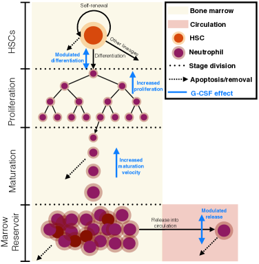
To maintain basal circulating neutrophil concentrations, multipotent progenitor HSCs in the bone marrow differentiate into the myeloid lineage on their way to becoming circulating neutrophils. After commitment, cells proliferate and undergo several divisions during a phase where cell numbers increase exponentially. After proliferation, neutrophil progenitors no longer divide. Instead, they grow in size and number of receptors before being sequestered into a marrow reservoir Rankin2010a , where they either die through apoptosis or transit into circulation Christopher2007 . Once they exit from the bone marrow, neutrophils circulate very transiently, with a half-removal time on the order of 7-10 hours VonVietinghoff2008 , as they either rapidly die or marginate into tissues Rankin2010a . Granulopoiesis is controlled by various cytokines, of which granulocyte colony-stimulating factor (G-CSF) is the principal actor Ward1999a . By binding to receptors on the neutrophil membranes, G-CSF regulates the rate at which neutrophils are released into circulation, and modulates up-stream factors (differentiation into the myeloid lineage, proliferation of upstream neutrophil progenitors, speed of maturation) to replenish and regulate the concentration of neutrophils in the bone marrow reservoir. G-CSF is then internalised by the neutrophils and removed from circulation. In the case of elevated circulating concentrations, G-CSF is also cleared via a linear, renal pathway Lyman2011 and these dual routes of elimination are important determinants of the PKs of G-CSF Craig2016c . An overview of the process of neutrophil production is given in Figure 1.
Refer to caption
Figure 1: An overview of granulopoiesis. As with all blood cells, neutrophils begin as hematopoietic stem cells (HSCs–orange circle) in the bone marrow (pale yelow background), where they develop. HSCs are capable of self-renewal and are subject to cell death (dashed arrows). HSCs may also differentiate into one of the blood cell lines, including the neutrophils (purple circles). After commitment to the neutrophil lineage, cells undergo a period of proliferative expansion after which they no longer divide. Post-mitotic neutrophils then mature, growing in size and gaining receptors. At the end of the maturation process, cells are then stored in the bone marrow reservoir from which they egress to reach circulation (pale red background) before removal (by margination or death). G-CSF acts to modulate the rate of exit from the marrow reservoir, increase the rates of maturation and proliferation, and to modulate the rate of differentiation into the neutrophil lineage (G-CSF actions represented by blue vertical arrows). Figure reproduced from “Towards quantitative systems pharmacology models of chemotherapy-induced neutropenia”, CPT: Pharmacometrics and Systems Pharmacology, 2017 (to appear), Craig, M., Craig2017 with the permission of Wiley.

Mathematical representations of granulopoiesis (and other similar physiological delay systems) fall into three classes: transit compartment models where delays are represented via a chain of first-order ordinary differential equations (ODEs), distributed delay systems where integro-differential equations represent a delay that takes a range of values determined through some probability distribution Campbell2009 ; Hearn1998 ; Adimy2007 ; Vainstein2005 , or delay differential equation (DDE) systems where the present state depends on past states via fixed or state-dependent delays Foley2008 ; Brooks2012 ; Craig2016c (for more detailed discussions on the various models used in modelling hematopoiesis and chemotherapy-induced neutropenia, see Pujo-Menjouet2016 and Craig2017 , respectively).

Here we focus on two models of granulopoiesis in particular: the Quartino model Quartino2014 and the Quantitative systems pharmacology (QSP) model of Craig Craig2016c . The Quartino transit compartment ODE model accounts for the effects and PKs of endogenous G-CSF and is an extension of the widely-used Friberg model Friberg2002 ; Friberg2003 , while the QSP granulopoiesis model of Craig2016c is a state-dependant delay DDE model that incorporates the concentrations of unbound G-CSF and G-CSF bound to its neutrophil receptors. We will show that the Quartino model Quartino2014 can be reformulated as a distributed delay DDE, which becomes a discrete-delay DDE in a certain parameter limit. This reformulation of the Quartino model leads to some additional insight on parameter choices and will lead us to generalise this model.

Since the maintenance of homeostasis or the pathogenic shift towards disease-states depend on the longterm behaviour of a given system’s steady states, stability is an integral concept in physiology. In what follows, we will study the stability of these three major granulopoiesis model-types (transit compartment, distributed and discrete delay, and QSP) by demonstrating the relationships and equivalencies between all three formalisms and analysing the resulting distributed delay model to provide a better understanding of the role model selection plays within a treatment context. Accordingly, we will discuss how these stability results can impact the incorporation and delineation of the effects of interindividual variability. We will also provide a historical context for the origins of transit compartment models from distributed delay models and DDEs.

This paper is divided as follows. We begin in Section 2.1 with an extension to the common ODE transit compartment model before introducing the more general distributed and discrete delay models in Section 2.2. Therein, we discuss the linear chain technique (Section 2.2.1) used to recover a transit compartment model from distributed delay systems. We then briefly introduce our previously published QSP model including endogenous G-CSF negative feedback in Section 2.3. The stability of the transit compartment/distributed/discrete delay models and the QSP model is analysed in Section 3 before we undertake bifurcation analyses (Section 4), which we discuss within the pharmaceutical sciences context in Section 5. We conclude by discussing our results in Section 6. Many of the proofs are provided in the appendices at the end.

2 Modelling granulopoiesis: three different approaches to handling delays

2.1 Transit compartment model with endogenous G-CSF

The Friberg model Friberg2002 is perhaps the most well-known model of myelosuppression after chemotherapy in the pharmaceutical sciences Craig2017 . Five compartments are used to represent the HSCs and early progenitors, circulating neutrophils, and the transit between the proliferative and circulative states. A feedback mechanism on the rate of proliferation determines the extent of myelosuppression of the chemotherapeutic agent. The model has been shown to generically represent a variety of chemotherapeutic drugs Friberg2003 and has been widely adopted in PK/PD studies of anti-cancer drugs. We write a generalised version of this model as

dPdtd𝑃d𝑡\displaystyle\frac{\textrm{d}P}{\textrm{d}t} =(kP(1EDrug)(N0N(t))γktr)Pabsentsubscript𝑘P1subscript𝐸Drugsuperscriptsubscript𝑁0𝑁𝑡𝛾subscript𝑘𝑡𝑟𝑃\displaystyle=\left(k_{\textit{\tiny P}}(1-E_{\textit{Drug}})\left(\frac{N_{0}}{N(t)}\right)^{\!\gamma}-k_{tr}\right)P
dT1dtdsubscript𝑇1d𝑡\displaystyle\frac{\textrm{d}T_{1}}{\textrm{d}t} =ktrPaT1absentsubscript𝑘𝑡𝑟𝑃𝑎subscript𝑇1\displaystyle=k_{tr}P-aT_{1} (2.1)
dTjdtdsubscript𝑇𝑗d𝑡\displaystyle\frac{\textrm{d}T_{j}}{\textrm{d}t} =a(Tj1Tj),j=2,,nformulae-sequenceabsent𝑎subscript𝑇𝑗1subscript𝑇𝑗𝑗2𝑛\displaystyle=a(T_{j-1}-T_{j}),\qquad j=2,\ldots,n
dNdtd𝑁d𝑡\displaystyle\frac{\textrm{d}N}{\textrm{d}t} =aTnkcircN,absent𝑎subscript𝑇𝑛subscript𝑘circ𝑁\displaystyle=aT_{n}-k_{\textit{circ}}N,

which reduces to the Friberg model if we set kP=ktr=asubscript𝑘Psubscript𝑘𝑡𝑟𝑎k_{\textit{\tiny P}}=k_{tr}=a and n=3𝑛3n=3. Here, P𝑃P is the concentration of proliferating progenitors, Tjsubscript𝑇𝑗T_{j} is the jthsuperscript𝑗thj^{\text{th}} post-mitotic transit compartment, and N𝑁N is the circulating neutrophil concentration (all in units of 109 cells/L), while kPsubscript𝑘Pk_{\textit{\tiny P}} is the rate of proliferation in the progenitor cell pool, ktrsubscript𝑘𝑡𝑟k_{tr} and a𝑎a are the transit rates between the maturation compartments, and kcircsubscript𝑘circk_{\textit{circ}} is the rate of neutrophil exit from circulation (all in units of h-1).
Refer to caption
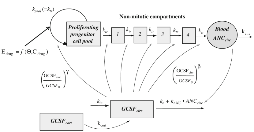
Figure 2: The integrated G-CSF-myelosuppression model describing the dynamics of endogenous G-CSF and neutrophils following chemotherapy. For the myelosuppression model the parameters are baseline neutrophil count (ANC0), mean maturation time (MMT=5/ktrtr{}_{\text{tr}}), the half-life of neutrophils in circulation (t1/2circsubscript12circ{}_{\nicefrac{{1}}{{2}}_{\text{circ}}}=ln\ln(2)/kcircsubscript𝑘circk_{\textit{circ}}), the feedback parameters of G-CSF on neutrophil proliferation (γ𝛾\gamma) and transit time (β𝛽\beta) and the drug related effect (Edrugdrug{}_{\text{drug}}). The estimated parameters for the G-CSF turnover model are baseline G-CSF (GCSF0), nonspecific elimination rate constant (kee{}_{\text{e}}) and ANC-dependent elimination rate constant (kANCsubscript𝑘ANCk_{\textit{\tiny ANC}}) and cortisol-induced G-CSF release (DOSEcortcort{}_{\text{cort}}) and the half-life of cortisol-induced G-CSF release (t1/2cortsubscript12cort{}_{\nicefrac{{1}}{{2}}_{\text{cort}}}=ln(2)/kcort2subscript𝑘cort\ln(2)/k_{\text{cort}}). Figure reproduced from “Characterization of endogenous G-CSF and the inverse correlation to chemotherapy-induced neutropenia in patients with breast cancer using population modeling”, Pharmaceutical Research, 31, 2014, pp. 3396, Quartino, A.L. et al., Quartino2014 with the permission of Springer.

An extension to the Friberg model, which we will refer to as the Quartino model, is presented in Quartino2014 and models the myelosuppressive effects of chemotherapy on progenitor and circulating neutrophils, the endogenous G-CSF response, and the effect of the administration of a glucocorticoid to induce a rapid increase in G-CSF. A model schematic is given in Figure 2. For our purposes, we can discount the administration of the glucocorticoid prior to chemotherapy and ignore the corresponding model terms. We write a generalised version of the model as

dPdtd𝑃d𝑡\displaystyle\frac{\textrm{d}P}{\textrm{d}t} =P(kP(1EDrug)(GG0)γktr(GG0)β)absent𝑃subscript𝑘P1subscript𝐸Drugsuperscript𝐺subscript𝐺0𝛾subscript𝑘𝑡𝑟superscript𝐺subscript𝐺0𝛽\displaystyle=P\left(k_{\textit{\tiny P}}(1-E_{\textit{Drug}})\left(\frac{G}{G_{0}}\right)^{\gamma}-k_{tr}\left(\frac{G}{G_{0}}\right)^{\beta}\right) (2.2a)
dT1dtdsubscript𝑇1d𝑡\displaystyle\frac{\textrm{d}T_{1}}{\textrm{d}t} =(GG0)β(ktrPaT1)absentsuperscript𝐺subscript𝐺0𝛽subscript𝑘𝑡𝑟𝑃𝑎subscript𝑇1\displaystyle=\left(\frac{G}{G_{0}}\right)^{\beta}(k_{tr}P-aT_{1}) (2.2b)
dTjdtdsubscript𝑇𝑗d𝑡\displaystyle\frac{\textrm{d}T_{j}}{\textrm{d}t} =a(GG0)β(Tj1Tj),j=2,,nformulae-sequenceabsent𝑎superscript𝐺subscript𝐺0𝛽subscript𝑇𝑗1subscript𝑇𝑗𝑗2𝑛\displaystyle=a\left(\frac{G}{G_{0}}\right)^{\beta}(T_{j-1}-T_{j}),\qquad j=2,\ldots,n (2.2c)
dNdtd𝑁d𝑡\displaystyle\frac{\textrm{d}N}{\textrm{d}t} =a(GG0)βTnkcircNabsent𝑎superscript𝐺subscript𝐺0𝛽subscript𝑇𝑛subscript𝑘circ𝑁\displaystyle=a\left(\frac{G}{G_{0}}\right)^{\beta}T_{n}-k_{\textit{circ}}N (2.2d)
dGdtd𝐺d𝑡\displaystyle\frac{\textrm{d}G}{\textrm{d}t} =kin(ke+kANCN)G,absentsubscript𝑘𝑖𝑛subscript𝑘𝑒subscript𝑘ANC𝑁𝐺\displaystyle=k_{in}-(k_{e}+k_{\textit{\tiny ANC}}N)G, (2.2e)

where G𝐺G is the circulating G-CSF concentration (ng/L), kANCsubscript𝑘ANCk_{\textit{\tiny ANC}} is the neutrophil-dependent rate of G-CSF elimination (h-1), kesubscript𝑘𝑒k_{e} is the G-CSF nonspecific elimination rate (h-1), (G/G0)γsuperscript𝐺subscript𝐺0𝛾(G/G_{0})^{\gamma} is the feedback on the proliferation rate from circulating G-CSF concentrations, and (G/G0)βsuperscript𝐺subscript𝐺0𝛽(G/G_{0})^{\beta} reflects the G-CSF feedback on the maturation rate. In most of the current work we do not consider the chemotherapeutic agent and set EDrug=0subscript𝐸Drug0E_{\textit{Drug}}=0, unless otherwise stated.

We let P0subscript𝑃0P_{0}, N0subscript𝑁0N_{0} and G0subscript𝐺0G_{0} denote the homeostasis values of P𝑃P, N𝑁N and G𝐺G respectively, obtained by setting

dPdt=dTjdt=dNdt=dGdt=0d𝑃d𝑡dsubscript𝑇𝑗d𝑡d𝑁d𝑡d𝐺d𝑡0\frac{\textrm{d}P}{\textrm{d}t}=\frac{\textrm{d}T_{j}}{\textrm{d}t}=\frac{\textrm{d}N}{\textrm{d}t}=\frac{\textrm{d}G}{\textrm{d}t}=0 (2.3)

in (2.2). In both the Friberg and Quartino models, it is a modelling assumption that

kP=ktr.subscript𝑘Psubscript𝑘𝑡𝑟k_{\textit{\tiny P}}=k_{tr}. (2.4)

The condition (2.4) is required in the Friberg model (2.1) to ensure that N=N0𝑁subscript𝑁0N=N_{0} at homeostasis, and in the Quartino model (2.2) to ensure that G=G0𝐺subscript𝐺0G=G_{0} at homeostasis. If G0subscript𝐺0G_{0} were not the homeostasis value of G𝐺G, it would be hard to justify the (G/G0)βsuperscript𝐺subscript𝐺0𝛽(G/G_{0})^{\beta} terms appearing throughout the model, and the model ought to take a different form. Consequently we enforce the condition (2.4) throughout, and always assume that ktr=kPsubscript𝑘𝑡𝑟subscript𝑘Pk_{tr}=k_{\textit{\tiny P}} as in Quartino2014 .

To see why we generalise the model by including a new parameter a𝑎a, note that at homeostasis the rate of production of proliferating cells, the rate that cells leave proliferation to enter the first transit compartment, the rate they leave the last transit compartment to enter circulation and the rate that they leave circulation must all be equal. In both models this results in

kPP0=ktrP0=kcircN0.subscript𝑘Psubscript𝑃0subscript𝑘𝑡𝑟subscript𝑃0subscript𝑘circsubscript𝑁0k_{\textit{\tiny P}}P_{0}=k_{tr}P_{0}=k_{\textit{circ}}N_{0}. (2.5)

The production rate in (2.5) is completely independent of the maturation time of the cells; provided cells both enter and leave maturation at the rate given by (2.5), changing the maturation time τ𝜏\tau would only change the total number of cells that are in maturation (which is τkPP0𝜏subscript𝑘Psubscript𝑃0\tau k_{\textit{\tiny P}}P_{0}), but will not change the production rate in (2.5). We will see below that at homeostasis the maturation time τ𝜏\tau for both models is given by

τ=na.𝜏𝑛𝑎\tau=\frac{n}{a}. (2.6)

Fixing a=ktr𝑎subscript𝑘𝑡𝑟a=k_{tr} leads to two related modelling problems. First if we regard a=ktr𝑎subscript𝑘𝑡𝑟a=k_{tr} as known then, since n𝑛n is an integer, equation (2.6) only allows for certain discrete values of the delay τ𝜏\tau. On the other hand, if as is more usual we suppose that τ𝜏\tau is known then choosing n𝑛n an integer and imposing that a=ktr𝑎subscript𝑘𝑡𝑟a=k_{tr} in (2.6) uniquely determines the value of ktrsubscript𝑘𝑡𝑟k_{tr} in (2.6), which in turn determines the production rate in (2.5). But we already noted that the production rate at homeostasis kPP0subscript𝑘Psubscript𝑃0k_{\textit{\tiny P}}P_{0} and the maturation time τ𝜏\tau are independent.

Parameter Units Typical estimate (% RSE)
N0subscript𝑁0N_{0} 109 cells/L 3.53 (5)
ktr=kPsubscript𝑘𝑡𝑟subscript𝑘Pk_{tr}=k_{\textit{\tiny P}} h-1 0.03759
γ𝛾\gamma - 0.444 (4)
β𝛽\beta - 0.234 (8)
G0subscript𝐺0G_{0} ng/L 24.3 (8)
kesubscript𝑘𝑒k_{e} h-1 0.592 (32)
kANCsubscript𝑘ANCk_{\textit{\tiny ANC}} h/109 cells/L 5.64
kcircsubscript𝑘circk_{\textit{circ}} h-1 0.099
kinsubscript𝑘𝑖𝑛k_{in} h-1 498.1792
Table 1: Parameter values from Quartino2014 for the parameters of interest in this study. The mean value of the distributed delay in (2.31) is given by τ=n/a𝜏𝑛𝑎\tau=n/a, or τ=106.41𝜏106.41\tau=106.41 hours.

In Quartino Quartino2014 a mean maturation time is defined by MMT=(n+1)/ktr𝑀𝑀𝑇𝑛1subscript𝑘𝑡𝑟MMT=(n+1)/k_{tr}. Presumably the authors counted n𝑛n transit compartments plus one proliferation compartment. By showing the equivalence of the generalised Quartino model (2.2) to a distributed delay DDE in Section 2.2 we will find both the mean and variance of the delay, and show that even if a=ktr𝑎subscript𝑘𝑡𝑟a=k_{tr} the correct formula for the mean maturation time should be MMT=n/ktr𝑀𝑀𝑇𝑛subscript𝑘𝑡𝑟MMT=n/k_{tr}, corresponding to (2.6), and not the formula used in Quartino Quartino2014 .

In the following sections we will consider general values of the parameters a𝑎a and n𝑛n, but will take the values of the remaining parameters from Quartino2014 ; these values are tabulated in Table 1. To satisfy the homeostasis conditions (2.3) we obtain

Tj=N0kcirca,j=1,,n,P0=N0kcircktr,formulae-sequencesubscript𝑇𝑗subscript𝑁0subscript𝑘circ𝑎formulae-sequence𝑗1𝑛subscript𝑃0subscript𝑁0subscript𝑘circsubscript𝑘𝑡𝑟T_{j}=\frac{N_{0}k_{\textit{circ}}}{a},\;j=1,\ldots,n,\qquad P_{0}=\frac{N_{0}k_{\textit{circ}}}{k_{tr}}, (2.7)

and the parameter constraint

kin=G0(ke+kANCN0).subscript𝑘𝑖𝑛subscript𝐺0subscript𝑘𝑒subscript𝑘ANCsubscript𝑁0k_{in}=G_{0}(k_{e}+k_{\textit{\tiny ANC}}N_{0}). (2.8)

At homeostasis the total number of cells in the n𝑛n maturation compartments is N0kcircn/asubscript𝑁0subscript𝑘circ𝑛𝑎N_{0}k_{\textit{circ}}n/a. Dividing this by the production rate given by (2.5) gives the average maturation time τ=n/a𝜏𝑛𝑎\tau=n/a as stated in (2.6).

Notice that if a=ktr𝑎subscript𝑘𝑡𝑟a=k_{tr} as in Quartino2014 then at steady state we have Tj=Psubscript𝑇𝑗𝑃T_{j}=P for all the transit compartments. In Quartino2014 the model (2.2) is considered with initial conditions at time t=0𝑡0t=0 equal to the steady-state values (which is natural for a chemotherapy study before the chemotherapeutic agent is administered), but we will consider the behaviour of the model for general non-negative initial conditions. Proof of the positivity of solutions to the Quartino system (2.2) can be found in Appendix B.1.

2.2 Gamma-distributed delay representation of the transit compartment granulopoiesis models

Distributed delay DDEs come in many varieties, but a reasonably general form is

dNdtd𝑁d𝑡\displaystyle\frac{\textrm{d}N}{\textrm{d}t} =f(t,N(t),tP(s)gap(ts)𝑑s)absent𝑓𝑡𝑁𝑡superscriptsubscript𝑡𝑃𝑠superscriptsubscript𝑔𝑎𝑝𝑡𝑠differential-d𝑠\displaystyle=f\!\left(t,N(t),\!\int_{-\infty}^{t}P(s)g_{a}^{p}(t-s)ds\right) (2.9)
=f(t,N(t),0P(tu)gap(u)𝑑u).absent𝑓𝑡𝑁𝑡superscriptsubscript0𝑃𝑡𝑢superscriptsubscript𝑔𝑎𝑝𝑢differential-d𝑢\displaystyle=f\!\left(t,N(t),\!\int_{0}^{\infty}P(t-u)g_{a}^{p}(u)du\right).

In simpler examples P(t)N(t)𝑃𝑡𝑁𝑡P(t)\equiv N(t), but P(t)𝑃𝑡P(t) can also be a separate variable defined by its own differential equation (as is the case in the granulopoiesis models considered in this work). The function gap(u)superscriptsubscript𝑔𝑎𝑝𝑢g_{a}^{p}(u) is a probability density with

0gap(u)𝑑u=1.superscriptsubscript0superscriptsubscript𝑔𝑎𝑝𝑢differential-d𝑢1\int_{0}^{\infty}g_{a}^{p}(u)du=1. (2.10)

So, rather than the dynamics of N(t)𝑁𝑡N(t) being determined by the current value of P(t)𝑃𝑡P(t), the integral distributes the effect of P𝑃P across its previous values. In this work we will restrict attention to the gamma distribution, though other distributions do arise, in particular the uniform distribution. We write the probability density function gapsuperscriptsubscript𝑔𝑎𝑝g_{a}^{p} of the gamma distribution as

gap(t)=aptp1eatΓ(p),superscriptsubscript𝑔𝑎𝑝𝑡superscript𝑎𝑝superscript𝑡𝑝1superscript𝑒𝑎𝑡Γ𝑝g_{a}^{p}(t)=\frac{a^{p}t^{p-1}e^{-at}}{\Gamma(p)}, (2.11)

where Γ(p)Γ𝑝\Gamma(p) is the gamma function. When n𝑛n is a positive integer Γ(n)=(n1)!Γ𝑛𝑛1\Gamma(n)=(n-1)!, and the gamma function generalises the factorial function to real numbers p𝑝p with Γ(p)=(p1)Γ(p1)Γ𝑝𝑝1Γ𝑝1\Gamma(p)=(p-1)\Gamma(p-1) for any p>0𝑝0p>0. The real positive parameters a𝑎a and p𝑝p determine the shape and rate of the distribution with the mean delay τ𝜏\tau given by

τ=p/a,𝜏𝑝𝑎\tau=p/a, (2.12)

and standard deviation σ2=p/a2superscript𝜎2𝑝superscript𝑎2\sigma^{2}=p/a^{2}. If p𝑝p and a𝑎a are taken to infinity with their ratio τ𝜏\tau held constant then the variance decreases to zero and the probability density function gap(t)superscriptsubscript𝑔𝑎𝑝𝑡g_{a}^{p}(t) becomes narrower and taller and approaches the δ𝛿\delta-function δ(tτ)𝛿𝑡𝜏\delta(t-\tau). In this limit the distributed delay DDE (2.9) reduces to a discrete delay DDE

dNdt=f(t,N(t),P(tτ)).d𝑁d𝑡𝑓𝑡𝑁𝑡𝑃𝑡𝜏\frac{\textrm{d}N}{\textrm{d}t}=f(t,N(t),P(t-\tau)). (2.13)

So discrete delay DDEs can be thought of as a limiting case of distributed delay DDEs. We will see below that when p=n𝑝𝑛p=n an integer, we can rewrite a gamma distributed DDE as an ODE, so gamma distributed DDEs provide a link between ODEs and discrete delay DDE models.

2.2.1 The Linear Chain Technique

The linear chain technique is used to convert some distributed delay differential equations (DDEs) into a corresponding system of ordinary differential equations (ODEs), or vice versa. The technique dates back at least to the work of Vogel in the 1960s Vogel63 ; Vogel65 , and first appears in the English literature in the work of MacDonald MacDonald78 ; MacDonald89 who called the method the linear chain trick. Most authors continue to use that name, but we prefer linear chain technique, because, as we will see, there is a true equivalency between the differential equation systems, and no trick is involved. It is usually more convenient to formulate problems as ODEs for numerical simulation, but sometimes more convenient to formulate them as DDEs for analysis. The linear chain technique is well-known and used in population biology and mathematical epidemiology, but is as yet not as well-known in other fields. The method has been independently rediscovered several times over the decades, being referred to as the fixed boxcartrain method by Goudriaan Goudriaan1986 , and recently used by Krzyzanski Krzyzanski2011 in a pharmaceutical sciences setting. There are several variants on this technique, and descriptions can be found in many places including Jacquez2002 ; MacDonald89 ; Smith2011 , but the simplest application is for a gamma distributed delay, for which we will detail the steps here.

The probability density function (2.11) has the property that for p1𝑝1p\neq 1

ddtgap(t)dd𝑡superscriptsubscript𝑔𝑎𝑝𝑡\displaystyle\frac{\textrm{d}}{\textrm{d}t}g_{a}^{p}(t) =(p1)aptp2eatΓ(p)ap+1tp1eatΓ(p)absent𝑝1superscript𝑎𝑝superscript𝑡𝑝2superscript𝑒𝑎𝑡Γ𝑝superscript𝑎𝑝1superscript𝑡𝑝1superscript𝑒𝑎𝑡Γ𝑝\displaystyle=\frac{(p-1)a^{p}t^{p-2}e^{-at}}{\Gamma(p)}-\frac{a^{p+1}t^{p-1}e^{-at}}{\Gamma(p)}
=a(ap1tp2eatΓ(p1)aptp1eatΓ(p))absent𝑎superscript𝑎𝑝1superscript𝑡𝑝2superscript𝑒𝑎𝑡Γ𝑝1superscript𝑎𝑝superscript𝑡𝑝1superscript𝑒𝑎𝑡Γ𝑝\displaystyle=a\left(\frac{a^{p-1}t^{p-2}e^{-at}}{\Gamma(p-1)}-\frac{a^{p}t^{p-1}e^{-at}}{\Gamma(p)}\right)
=a(gap1(t)gap(t)).absent𝑎superscriptsubscript𝑔𝑎𝑝1𝑡superscriptsubscript𝑔𝑎𝑝𝑡\displaystyle=a(g_{a}^{p-1}(t)-g_{a}^{p}(t)). (2.14)

While for p=1𝑝1p=1

ddtga1(t)=ddt(aeat)=aga1(t).dd𝑡superscriptsubscript𝑔𝑎1𝑡dd𝑡𝑎superscript𝑒𝑎𝑡𝑎superscriptsubscript𝑔𝑎1𝑡\frac{\textrm{d}}{\textrm{d}t}g_{a}^{1}(t)=\frac{\textrm{d}}{\textrm{d}t}(ae^{-at})=-ag_{a}^{1}(t). (2.15)

Models of the form (2.9),(2.11) can in principle be considered for any real positive value of p𝑝p, but in practice nearly all authors only consider p=n𝑝𝑛p=n a positive integer (one exception is Campbell2009 ), because then equations (2.14),(2.15) allow the distributed DDE to be reduced to an ODE. To do this let

Tj(t)=tP(s)gaj(ts)𝑑s=0P(tu)gaj(u)𝑑u,j=1,,n.formulae-sequencesubscript𝑇𝑗𝑡superscriptsubscript𝑡𝑃𝑠superscriptsubscript𝑔𝑎𝑗𝑡𝑠differential-d𝑠superscriptsubscript0𝑃𝑡𝑢superscriptsubscript𝑔𝑎𝑗𝑢differential-d𝑢𝑗1𝑛T_{j}(t)=\int_{-\infty}^{t}P(s)g_{a}^{j}(t-s)\,ds=\int_{0}^{\infty}P(t-u)g_{a}^{j}(u)\,du,\qquad j=1,\ldots,n. (2.16)

Then equation (2.9) can be rewritten as an ODE

dNdt=f(t,N(t),Tn(t)).d𝑁d𝑡𝑓𝑡𝑁𝑡subscript𝑇𝑛𝑡\frac{\textrm{d}N}{\textrm{d}t}=f\left(t,N(t),T_{n}(t)\right). (2.17)

Differentiating (2.16), using Leibniz rule for j>1𝑗1j>1 (noting that gaj(0)=0superscriptsubscript𝑔𝑎𝑗00g_{a}^{j}(0)=0 for j>1𝑗1j>1) we obtain

dTjdtdsubscript𝑇𝑗d𝑡\displaystyle\frac{\textrm{d}T_{j}}{\textrm{d}t} =P(t)gaj(0)+tP(s)ddtgaj(ts)𝑑sabsent𝑃𝑡superscriptsubscript𝑔𝑎𝑗0superscriptsubscript𝑡𝑃𝑠dd𝑡superscriptsubscript𝑔𝑎𝑗𝑡𝑠differential-d𝑠\displaystyle=P(t)g_{a}^{j}(0)+\int_{-\infty}^{t}P(s)\frac{\textrm{d}}{\textrm{d}t}g_{a}^{j}(t-s)\,ds
=tP(s)a(gaj1(ts)gaj(ts))𝑑sabsentsuperscriptsubscript𝑡𝑃𝑠𝑎superscriptsubscript𝑔𝑎𝑗1𝑡𝑠superscriptsubscript𝑔𝑎𝑗𝑡𝑠differential-d𝑠\displaystyle=\int_{-\infty}^{t}P(s)a(g_{a}^{j-1}(t-s)-g_{a}^{j}(t-s))\,ds
=a(Tj1(t)Tj(t)),j={2,3,,n}.formulae-sequenceabsent𝑎subscript𝑇𝑗1𝑡subscript𝑇𝑗𝑡𝑗23𝑛\displaystyle=a(T_{j-1}(t)-T_{j}(t)),\quad j=\{2,3,\ldots,n\}. (2.18)

While for j=1𝑗1j=1 (noting that ga1(0)=asuperscriptsubscript𝑔𝑎10𝑎g_{a}^{1}(0)=a)

dT1dt=P(t)ga1(0)+tP(s)ddtga1(ts)𝑑s=a(P(t)T1(t)).dsubscript𝑇1d𝑡𝑃𝑡superscriptsubscript𝑔𝑎10superscriptsubscript𝑡𝑃𝑠dd𝑡superscriptsubscript𝑔𝑎1𝑡𝑠differential-d𝑠𝑎𝑃𝑡subscript𝑇1𝑡\frac{\textrm{d}T_{1}}{\textrm{d}t}=P(t)g_{a}^{1}(0)+\int_{-\infty}^{t}P(s)\frac{\textrm{d}}{\textrm{d}t}g_{a}^{1}(t-s)\,ds\\ =a(P(t)-T_{1}(t)). (2.19)

Together equations (2.17),(2.18),(2.19) redefine the (nonlinear) distributed delay DDE (2.9) as a system of n+1𝑛1n+1 ODEs. General DDEs can be posed as infinite dimensional dynamical systems, which introduces considerable mathematical difficulties, so being able to reduce some DDE models to finite-dimensional ODEs is mathematically very advantageous.

To complete the relationship between the distributed delay DDE (2.9) and the system of ODEs (2.17),(2.18),(2.19) we should take some care with the initial conditions. The distributed DDE (2.9) has infinite memory, and so to solve as an initial value problem from time t=0𝑡0t=0 we need to define a history function P(t)𝑃𝑡P(t) for all t0𝑡0t\leqslant 0, so that the right hand-side of (2.9) can be evaluated. With P(t)𝑃𝑡P(t) so defined, for the DDE and ODE reduction to have equivalent solutions, by (2.16) the ODE must have initial conditions

Tj(0)=0P(s)gaj(s)𝑑s=0P(s)gaj(s)𝑑sj=1,,n.formulae-sequencesubscript𝑇𝑗0superscriptsubscript0𝑃𝑠superscriptsubscript𝑔𝑎𝑗𝑠differential-d𝑠superscriptsubscript0𝑃𝑠superscriptsubscript𝑔𝑎𝑗𝑠differential-d𝑠𝑗1𝑛T_{j}(0)=\int_{-\infty}^{0}P(s)g_{a}^{j}(-s)\,ds=\int_{0}^{\infty}P(s)g_{a}^{j}(s)\,ds\qquad j=1,\ldots,n. (2.20)

If it is assumed that P(t)=P0𝑃𝑡subscript𝑃0P(t)=P_{0}, a constant for all t0𝑡0t\leqslant 0 then, using (2.10), we see that (2.20) reduces to

Tj(0)=P00gaj(s)𝑑s=P0,j=1,,n.formulae-sequencesubscript𝑇𝑗0subscript𝑃0superscriptsubscript0superscriptsubscript𝑔𝑎𝑗𝑠differential-d𝑠subscript𝑃0𝑗1𝑛T_{j}(0)=P_{0}\int_{0}^{\infty}g_{a}^{j}(s)\,ds=P_{0},\qquad j=1,\ldots,n. (2.21)

It is natural to ask if we can also go the other way; does a solution of the system of ODEs (2.17),(2.18),(2.19), define a solution of the distributed DDE (2.9)? It follows immediately from (2.21) that a solution of the ODE system with initial conditions P(0)=Tj(0)𝑃0subscript𝑇𝑗0P(0)=T_{j}(0) for j=1,,n𝑗1𝑛j=1,\ldots,n does define a solution of (2.9). The equivalence for more general initial conditions for the ODE has also been established; in that case the ODE initial conditions define a finite number of constraints on the history function P(t)𝑃𝑡P(t) for t0𝑡0t\leqslant 0, which do not uniquely define P(t)𝑃𝑡P(t), and the ODE defines a solution of the distributed DDE (2.9) for all choices of P(t)𝑃𝑡P(t) that satisfy the constraints Cooke1982 ; MacDonald89 .

2.2.2 Gamma-distributed and discrete delay representations of transit compartment granulopoiesis models

The linear chain technique of Section 2.2.1 can be applied to establish the equivalence between transit compartment ODE models and corresponding distributed delay DDEs. Consider first the distributed DDE system

dPdt=(kP(1EDrug)(N0N(t))γktr)PdNdt=kcircN+ktrtP(s)gan(ts)𝑑s.d𝑃d𝑡subscript𝑘P1subscript𝐸Drugsuperscriptsubscript𝑁0𝑁𝑡𝛾subscript𝑘𝑡𝑟𝑃formulae-sequenced𝑁d𝑡subscript𝑘circ𝑁subscript𝑘𝑡𝑟superscriptsubscript𝑡𝑃𝑠superscriptsubscript𝑔𝑎𝑛𝑡𝑠differential-d𝑠\begin{array}[]{l}\displaystyle\frac{\textrm{d}P}{\textrm{d}t}=\left(k_{\textit{\tiny P}}(1-E_{\textit{Drug}})\left(\frac{N_{0}}{N(t)}\right)^{\!\gamma}-k_{tr}\right)P\\ \displaystyle\frac{\textrm{d}N}{\textrm{d}t}=-k_{\textit{circ}}N+k_{tr}\!\int_{-\infty}^{t}P(s)g_{a}^{n}(t-s)ds.\rule[-2.84526pt]{0.0pt}{22.76219pt}\end{array} (2.22)

We define Tj(t)subscript𝑇𝑗𝑡T_{j}(t) by

Tj(t)=tktraP(s)gaj(ts)𝑑s,j=1,,n,formulae-sequencesubscript𝑇𝑗𝑡superscriptsubscript𝑡subscript𝑘𝑡𝑟𝑎𝑃𝑠superscriptsubscript𝑔𝑎𝑗𝑡𝑠differential-d𝑠𝑗1𝑛T_{j}(t)=\int_{-\infty}^{t}\frac{k_{tr}}{a}P(s)g_{a}^{j}(t-s)\,ds,\qquad j=1,\ldots,n, (2.23)

which corresponds to (2.16) with ktrP(s)/asubscript𝑘𝑡𝑟𝑃𝑠𝑎k_{tr}P(s)/a replacing P(s)𝑃𝑠P(s). Writing the equation for N(t)𝑁𝑡N(t) as

dNdt=kcircN+atktraP(s)gan(ts)𝑑s,d𝑁d𝑡subscript𝑘circ𝑁𝑎superscriptsubscript𝑡subscript𝑘𝑡𝑟𝑎𝑃𝑠superscriptsubscript𝑔𝑎𝑛𝑡𝑠differential-d𝑠\frac{\textrm{d}N}{\textrm{d}t}=-k_{\textit{circ}}N+a\!\int_{-\infty}^{t}\frac{k_{tr}}{a}P(s)g_{a}^{n}(t-s)ds, (2.24)

and applying the linear chain technique of Section 2.2.1 we obtain the generalised Friberg transition compartment model of myelosuppression (2.1). Taking a=ktr𝑎subscript𝑘𝑡𝑟a=k_{tr} and n=3𝑛3n=3 gives the Friberg model as stated in Friberg2002 , as has already been noted in Belair2015 .

While it is necessary to set a=ktr𝑎subscript𝑘𝑡𝑟a=k_{tr} in (2.22) to recover the model as stated in Friberg2002 , equation (2.1) defines a transit compartment model for other values of a𝑎a also, and both the system of ODEs (2.1) and the distributed DDE (2.22) can be considered for general values a>0𝑎0a>0.

The extended Quartino endogenous G-CSF model Quartino2014 as stated in (2.2) and discussed in Section 2.1 cannot be stated simply as a distributed delay DDE via the linear chain technique. The maturation time in the Quartino model instead of being constant is state-dependent with the rate constants for the passage through each transit compartment given by

a(G(t)G0)β,𝑎superscript𝐺𝑡subscript𝐺0𝛽a\left(\frac{G(t)}{G_{0}}\right)^{\beta},

which varies as G(t)𝐺𝑡G(t) varies; it reduces to the same value as for the Friberg model only if G(t)=G0𝐺𝑡subscript𝐺0G(t)=G_{0}. In contrast, the derivation of (2.14), which is essential in the linear chain technique, requires that the rate constant a𝑎a (and the power p𝑝p) be constant, so to apply the linear chain technique the profile of the probability density function must remain constant and cannot vary with time or the solution. Thus, while it might be tempting to consider a distributed DDE of the form

dPdt=P(kP(GG0)γktr(GG0)β)dNdt=kcircN+ktr(GG0)βtP(s)gan(ts)𝑑sdGdt=kin(ke+kANCN)G,d𝑃d𝑡𝑃subscript𝑘Psuperscript𝐺subscript𝐺0𝛾subscript𝑘𝑡𝑟superscript𝐺subscript𝐺0𝛽d𝑁d𝑡subscript𝑘circ𝑁subscript𝑘𝑡𝑟superscript𝐺subscript𝐺0𝛽superscriptsubscript𝑡𝑃𝑠superscriptsubscript𝑔𝑎𝑛𝑡𝑠differential-d𝑠d𝐺d𝑡subscript𝑘𝑖𝑛subscript𝑘𝑒subscript𝑘ANC𝑁𝐺\begin{split}\frac{\textrm{d}P}{\textrm{d}t}&=P\left(k_{\textit{\tiny P}}\left(\frac{G}{G_{0}}\right)^{\gamma}-k_{tr}\left(\frac{G}{G_{0}}\right)^{\beta}\right)\\ \frac{\textrm{d}N}{\textrm{d}t}&=-k_{\textit{circ}}N+k_{tr}\left(\frac{G}{G_{0}}\right)^{\beta}\int_{-\infty}^{t}P(s)g_{a}^{n}(t-s)\,ds\\ \frac{\textrm{d}G}{\textrm{d}t}&=k_{in}-(k_{e}+k_{\textit{\tiny ANC}}N)G,\end{split} (2.25)

if we set a=ktr(G(t))/G0)βa=k_{tr}(G(t))/G_{0})^{\beta}, then it is not possible to reduce this model to a system of ODEs because the derivation of (2.14) fails when a𝑎a is time-dependent. Instead we could consider the model

dPdt=P(kP(GG0)γktr(GG0)β)dNdt=kcircN+ktrt(G(s)G0)βP(s)gan(ts)𝑑sdGdt=kin(ke+kANCN)G,d𝑃d𝑡𝑃subscript𝑘Psuperscript𝐺subscript𝐺0𝛾subscript𝑘𝑡𝑟superscript𝐺subscript𝐺0𝛽d𝑁d𝑡subscript𝑘circ𝑁subscript𝑘𝑡𝑟superscriptsubscript𝑡superscript𝐺𝑠subscript𝐺0𝛽𝑃𝑠superscriptsubscript𝑔𝑎𝑛𝑡𝑠differential-d𝑠d𝐺d𝑡subscript𝑘𝑖𝑛subscript𝑘𝑒subscript𝑘ANC𝑁𝐺\begin{split}\frac{\textrm{d}P}{\textrm{d}t}&=P\left(k_{\textit{\tiny P}}\left(\frac{G}{G_{0}}\right)^{\gamma}-k_{tr}\left(\frac{G}{G_{0}}\right)^{\beta}\right)\\ \frac{\textrm{d}N}{\textrm{d}t}&=-k_{\textit{circ}}N+k_{tr}\int_{-\infty}^{t}\left(\frac{G(s)}{G_{0}}\right)^{\beta}P(s)g_{a}^{n}(t-s)\,ds\\ \frac{\textrm{d}G}{\textrm{d}t}&=k_{in}-(k_{e}+k_{\textit{\tiny ANC}}N)G,\end{split} (2.26)

and apply the linear chain technique with

Tj(t)=tktra(G(s)G0)βP(s)gaj(ts)𝑑s,j=1,,n.formulae-sequencesubscript𝑇𝑗𝑡superscriptsubscript𝑡subscript𝑘𝑡𝑟𝑎superscript𝐺𝑠subscript𝐺0𝛽𝑃𝑠superscriptsubscript𝑔𝑎𝑗𝑡𝑠differential-d𝑠𝑗1𝑛T_{j}(t)=\int_{-\infty}^{t}\frac{k_{tr}}{a}\left(\frac{G(s)}{G_{0}}\right)^{\beta}P(s)g_{a}^{j}(t-s)\,ds,\qquad j=1,\ldots,n. (2.27)

to obtain the transit compartment model

dPdt=P(kP(GG0)γktr(GG0)β)dT1dt=ktr(GG0)βP(t)aT1(t)dTjdt=a(Tj1(t)Tj(t)),j={2,3,,n}dNdt=aTn(t)kcircNdGdt=kin(ke+kANCN)G,\begin{split}\frac{\textrm{d}P}{\textrm{d}t}&=P\left(k_{\textit{\tiny P}}\left(\frac{G}{G_{0}}\right)^{\gamma}-k_{tr}\left(\frac{G}{G_{0}}\right)^{\beta}\right)\\ \frac{\textrm{d}T_{1}}{\textrm{d}t}&=k_{tr}\left(\frac{G}{G_{0}}\right)^{\beta}P(t)-aT_{1}(t)\\ \frac{\textrm{d}T_{j}}{\textrm{d}t}&=a(T_{j-1}(t)-T_{j}(t)),\quad j=\{2,3,\ldots,n\}\\ \frac{\textrm{d}N}{\textrm{d}t}&=aT_{n}(t)-k_{\textit{circ}}N\\ \frac{\textrm{d}G}{\textrm{d}t}&=k_{in}-(k_{e}+k_{\textit{\tiny ANC}}N)G,\end{split} (2.28)

which is similar to the Quartino model (2.2), but missing the (G(t)/G0)βsuperscript𝐺𝑡subscript𝐺0𝛽(G(t)/G_{0})^{\beta} factors in all the Tjsubscript𝑇𝑗T_{j} transit terms, and consequently does not model the effect of G-CSF on the maturation rate.

To write the Quartino model (2.2) as a distributed DDE, we first remove the state-dependency of the delays by rescaling time. Define a new time t^(t)^𝑡𝑡\hat{t}(t) by

dt^dt=(G(t)G0)β,t^(0)=0.formulae-sequenced^𝑡d𝑡superscript𝐺𝑡subscript𝐺0𝛽^𝑡00\frac{\textrm{d}\hat{t}}{\textrm{d}t}=\left(\frac{G(t)}{G_{0}}\right)^{\beta},\qquad\hat{t}(0)=0. (2.29)

By Theorem B.1 the right-hand side of (2.29) is strictly positive for t>0𝑡0t>0 so dt^dt>0d^𝑡d𝑡0\frac{\textrm{d}\hat{t}}{\textrm{d}t}>0 and the new time variable t^(t)^𝑡𝑡\hat{t}(t) is a strictly monotonic increasing function of t𝑡t. Then we see that

dTjdt^=dtdt^dTjdt=(G0G(t^))βa(G(t^)G0)β(Tj1Tj)=a(Tj1Tj).dsubscript𝑇𝑗d^𝑡d𝑡d^𝑡dsubscript𝑇𝑗d𝑡superscriptsubscript𝐺0𝐺^𝑡𝛽𝑎superscript𝐺^𝑡subscript𝐺0𝛽subscript𝑇𝑗1subscript𝑇𝑗𝑎subscript𝑇𝑗1subscript𝑇𝑗\frac{\textrm{d}T_{j}}{\textrm{d}\hat{t}}=\frac{\textrm{d}t}{\textrm{d}\hat{t}}\frac{\textrm{d}T_{j}}{\textrm{d}t}=\left(\frac{G_{0}}{G(\hskip 0.50003pt\hat{t}\hskip 0.50003pt)}\right)^{\beta}a\left(\frac{G(\hskip 0.50003pt\hat{t}\hskip 0.50003pt)}{G_{0}}\right)^{\beta}(T_{j-1}-T_{j})=a(T_{j-1}-T_{j}).

Strictly speaking we should define new variables G~(t^)=G(t)~𝐺^𝑡𝐺𝑡\widetilde{G}(\hskip 0.50003pt\hat{t}\hskip 0.50003pt)=G(t), but following common practice we suppress the tildes and reuse the same variable names. Applying the same time-rescaling to all the equations we rewrite the Quartino model (2.2) as

dPdt^=(kP(G(t^)G0)γβktr)P(t^)dT1dt^=ktrP(t^)aT1(t^)dTjdt^=a(Tj1(t^)Tj(t^)),j=2,,ndNdt^=aTn(t^)(G0G(t^))βkcircN(t^)dGdt^=(G0G(t^))β(kin(ke+kANCN(t^))G(t^)).\begin{split}\frac{\textrm{d}P}{\textrm{d}\hat{t}}&=\left(k_{\textit{\tiny P}}\left(\frac{G(\hskip 0.50003pt\hat{t}\hskip 0.50003pt)}{G_{0}}\right)^{\gamma-\beta}-\,k_{tr}\right)P(\hskip 0.50003pt\hat{t}\hskip 0.50003pt)\\ \frac{\textrm{d}T_{1}}{\textrm{d}\hat{t}}&=k_{tr}P(\hskip 0.50003pt\hat{t}\hskip 0.50003pt)-aT_{1}(\hskip 0.50003pt\hat{t}\hskip 0.50003pt)\\ \frac{\textrm{d}T_{j}}{\textrm{d}\hat{t}}&=a(T_{j-1}(\hskip 0.50003pt\hat{t}\hskip 0.50003pt)-T_{j}(\hskip 0.50003pt\hat{t}\hskip 0.50003pt)),\qquad j=2,\ldots,n\\ \frac{\textrm{d}N}{\textrm{d}\hat{t}}&=aT_{n}(\hskip 0.50003pt\hat{t}\hskip 0.50003pt)-\left(\frac{G_{0}}{G(\hskip 0.50003pt\hat{t}\hskip 0.50003pt)}\right)^{\beta}k_{\textit{circ}}N(\hskip 0.50003pt\hat{t}\hskip 0.50003pt)\\ \frac{\textrm{d}G}{\textrm{d}\hat{t}}&=\left(\frac{G_{0}}{G(\hskip 0.50003pt\hat{t}\hskip 0.50003pt)}\right)^{\beta}\Bigl{(}k_{in}-(k_{e}+k_{\textit{\tiny ANC}}N(\hskip 0.50003pt\hat{t}\hskip 0.50003pt))G(\hskip 0.50003pt\hat{t}\hskip 0.50003pt)\Bigr{)}.\end{split} (2.30)

We refer to (2.30) as the time-rescaled Quartino model. Since the time rescaling satisfies t^(0)=0^𝑡00\hat{t}(0)=0, the initial conditions for the Quartino model (2.2) at t=0𝑡0t=0 and the time-rescaled Quartino model (2.30) at time t^=0^𝑡0\hat{t}=0 are the same, and these two equations given equivalent solutions.

The time-rescaled Quartino model (2.30) has constant transition rates between the transit compartments, and consequently we can apply the linear chain technique to derive (2.30) from

dPdt^=(kP(G(t^)G0)γβktr)P(t^)dNdt^=(G0G(t^))βkcircN(t^)+ktrt^P(s)gan(t^s)𝑑sdGdt^=(G0G(t^))β(kin(ke+kANCN(t^))G(t^)),d𝑃d^𝑡subscript𝑘Psuperscript𝐺^𝑡subscript𝐺0𝛾𝛽subscript𝑘𝑡𝑟𝑃^𝑡d𝑁d^𝑡superscriptsubscript𝐺0𝐺^𝑡𝛽subscript𝑘circ𝑁^𝑡subscript𝑘𝑡𝑟superscriptsubscript^𝑡𝑃𝑠superscriptsubscript𝑔𝑎𝑛^𝑡𝑠differential-d𝑠d𝐺d^𝑡superscriptsubscript𝐺0𝐺^𝑡𝛽subscript𝑘𝑖𝑛subscript𝑘𝑒subscript𝑘ANC𝑁^𝑡𝐺^𝑡\begin{split}\frac{\textrm{d}P}{\textrm{d}\hat{t}}&=\left(k_{\textit{\tiny P}}\left(\frac{G(\hskip 0.50003pt\hat{t}\hskip 0.50003pt)}{G_{0}}\right)^{\gamma-\beta}-k_{tr}\right)P(\hskip 0.50003pt\hat{t}\hskip 0.50003pt)\\ \frac{\textrm{d}N}{\textrm{d}\hat{t}}&=-\left(\frac{G_{0}}{G(\hskip 0.50003pt\hat{t}\hskip 0.50003pt)}\right)^{\beta}k_{\textit{circ}}N(\hskip 0.50003pt\hat{t}\hskip 0.50003pt)+k_{tr}\int_{-\infty}^{\hat{t}}P(s)g_{a}^{n}(\hat{t}-s)\,ds\\ \frac{\textrm{d}G}{\textrm{d}\hat{t}}&=\left(\frac{G_{0}}{G(\hskip 0.50003pt\hat{t}\hskip 0.50003pt)}\right)^{\beta}\Bigl{(}k_{in}-(k_{e}+k_{\textit{\tiny ANC}}N(\hskip 0.50003pt\hat{t}\hskip 0.50003pt))G(\hskip 0.50003pt\hat{t}\hskip 0.50003pt)\Bigr{)},\end{split} (2.31)

by letting

Tj(t^)=t^ktraP(s)gaj(t^s)𝑑s,j=1,,n.formulae-sequencesubscript𝑇𝑗^𝑡superscriptsubscript^𝑡subscript𝑘𝑡𝑟𝑎𝑃𝑠superscriptsubscript𝑔𝑎𝑗^𝑡𝑠differential-d𝑠𝑗1𝑛T_{j}(\hskip 0.50003pt\hat{t}\hskip 0.50003pt)=\int_{-\infty}^{\hat{t}}\frac{k_{tr}}{a}P(s)g_{a}^{j}(\hat{t}-s)\,ds,\qquad j=1,\ldots,n. (2.32)

To define an initial value problem for the distributed delay DDE (2.31) we need to specify N(0)𝑁0N(0), G(0)𝐺0G(0) and P(t^)𝑃^𝑡P(\hskip 0.50003pt\hat{t}\hskip 0.50003pt) for t^0^𝑡0\hat{t}\leqslant 0. This in turn defines initial conditions for both the time-rescaled Quartino model (2.30) and the Quartino model (2.2) with Tj(0)subscript𝑇𝑗0T_{j}(0) given by evaluating (2.32) with t^=0^𝑡0\hat{t}=0. If P(t^)𝑃^𝑡P(\hskip 0.50003pt\hat{t}\hskip 0.50003pt) is constant for t^0^𝑡0\hat{t}\leqslant 0 then (2.32) implies that Tj(0)=ktrP(0)/asubscript𝑇𝑗0subscript𝑘𝑡𝑟𝑃0𝑎T_{j}(0)=k_{tr}P(0)/a, so there is an immediate equivalence between all three models for such initial conditions. Even if the Quartino model (2.2) were considered with different initial conditions, there is still a direct equivalence to the time-rescaled Quartino model (2.30), and as noted at the end of Section 2.2.1, also to the distributed DDE model (2.31). Consequently we have three equivalent forms of the same model, with a direct correspondence between the solutions of the differential equation systems (2.2) and (2.30) and (2.31).

Recalling (2.12) the mean value of the distributed delay in (2.31) is τ=n/a𝜏𝑛𝑎\tau=n/a. The time rescaling (2.29) is trivial at homeostasis when G(t)=G0𝐺𝑡subscript𝐺0G(t)=G_{0}, so this also implies that the mean maturation delay is τ=n/a𝜏𝑛𝑎\tau=n/a in the Quartino model (2.2) (and fact that we already derived by a different argument in (2.6)). Fixing a=ktr𝑎subscript𝑘𝑡𝑟a=k_{tr} only allows a very granular control of the mean delay in the ODE model by varying the integer n𝑛n. Mathematically it is more convenient to fix the delay τ>0𝜏0\tau>0 and use n𝑛n and a𝑎a to control the shape of the distribution. For the distributed DDE model (2.31) we do not even need n𝑛n to be an integer. Recalling (2.10), in the limit as n𝑛n\to\infty and a𝑎a\to\infty with τ=n/a𝜏𝑛𝑎\tau=n/a fixed, the distributed delay DDE (2.31) reduces to the discrete delay DDE

dPdt^=(kP(G(t^)G0)γβktr)P(t^)dNdt^=(G0G(t^))βkcircN(t^)+ktrP(t^τ)dGdt^=(G0G(t^))β(kin(ke+kANCN(t^))G(t^)).d𝑃d^𝑡subscript𝑘Psuperscript𝐺^𝑡subscript𝐺0𝛾𝛽subscript𝑘𝑡𝑟𝑃^𝑡d𝑁d^𝑡superscriptsubscript𝐺0𝐺^𝑡𝛽subscript𝑘circ𝑁^𝑡subscript𝑘𝑡𝑟𝑃^𝑡𝜏d𝐺d^𝑡superscriptsubscript𝐺0𝐺^𝑡𝛽subscript𝑘𝑖𝑛subscript𝑘𝑒subscript𝑘ANC𝑁^𝑡𝐺^𝑡\begin{split}\frac{\textrm{d}P}{\textrm{d}\hat{t}}&=\left(k_{\textit{\tiny P}}\left(\frac{G(\hskip 0.50003pt\hat{t}\hskip 0.50003pt)}{G_{0}}\right)^{\gamma-\beta}-k_{tr}\right)P(\hskip 0.50003pt\hat{t}\hskip 0.50003pt)\\ \frac{\textrm{d}N}{\textrm{d}\hat{t}}&=-\left(\frac{G_{0}}{G(\hskip 0.50003pt\hat{t}\hskip 0.50003pt)}\right)^{\beta}k_{\textit{circ}}N(\hskip 0.50003pt\hat{t}\hskip 0.50003pt)+k_{tr}P(\hat{t}-\tau)\\ \frac{\textrm{d}G}{\textrm{d}\hat{t}}&=\left(\frac{G_{0}}{G(\hskip 0.50003pt\hat{t}\hskip 0.50003pt)}\right)^{\beta}\Bigl{(}k_{in}-(k_{e}+k_{\textit{\tiny ANC}}N(\hskip 0.50003pt\hat{t}\hskip 0.50003pt))G(\hskip 0.50003pt\hat{t}\hskip 0.50003pt)\Bigr{)}.\end{split} (2.33)

We remark that in the discrete delay DDE (2.33) the delay τ𝜏\tau is constant in the rescaled time-variable t^^𝑡\hat{t}, just as the (same) mean delay τ=n/a𝜏𝑛𝑎\tau=n/a is constant in the distributed delay DDE (2.31). In contrast the mean maturation time α(t)𝛼𝑡\alpha(t) in the Quartino model (2.2) varies with G(t)𝐺𝑡G(t) and satisfies

t^(tα(t))=t^(t)τ,^𝑡𝑡𝛼𝑡^𝑡𝑡𝜏\hat{t}(t-\alpha(t))=\hat{t}(t)-\tau,

where t^(t)^𝑡𝑡\hat{t}(t) satisfies (2.29). If G𝐺G is held constant (but not necessarily equal to G0subscript𝐺0G_{0}), this gives a mean maturation time α𝛼\alpha in the Quartino model (2.2) of

α=na(G/G0)β=τ(G/G0)β.𝛼𝑛𝑎superscript𝐺subscript𝐺0𝛽𝜏superscript𝐺subscript𝐺0𝛽\alpha=\frac{n}{a(G/G_{0})^{\beta}}=\frac{\tau}{(G/G_{0})^{\beta}}.

For the case of time-varying G(t)𝐺𝑡G(t), the evolution of the mean maturation delay α(t)𝛼𝑡\alpha(t) is defined by a differential equation (A.2), which we derive in Appendix A, where we also show the similarities between this state-dependency and the explicit state-dependency in the QSP model (2.34). But, in the current work, the time-rescaling equation (2.29) will be sufficient for our purposes.

Notice that while the derivation of (2.33) makes sense when considering the limit of the shape of the probability density functions gn/τn(t)superscriptsubscript𝑔𝑛𝜏𝑛𝑡g_{n/\tau}^{n}(t) as they approach the δ𝛿\delta-function δ(tτ)𝛿𝑡𝜏\delta(t-\tau) when n𝑛n\to\infty, it is problematical if one interprets the distributed DDE (2.31) via the ODE system (2.28) or (2.30) since then the limiting process would correspond to taking the number of compartments n𝑛n to infinity while increasing the rate constants a𝑎a to infinity also.

Since the system (2.30) corresponds to the Quartino model (2.2) with time rescaled by (2.26), positivity of solutions is guaranteed by Theorem B.1. The correspondence between the distributed delay system (2.31) and the system (2.30) ensures positivity of solutions of (2.31) for integer n𝑛n only, but actually positivity can be established for all real n>0𝑛0n>0. The proof of the positivity of solutions to (2.30) is given in Theorem B.2 in Appendix B.1.

2.3 A QSP model of granulopoiesis and its regulation by G-CSF

As previously mentioned, DDEs are frequently relied upon to model granulopoiesis given the delays inherent to hematopoiesis. Here we focus on the Quantitative systems pharmacology model of Craig2016c , which has been shown to account for the dynamics of neutrophil production and its negative feedback relationship with G-CSF–both bound to receptors on the surface of neutrophils and freely circulating–in a variety of scenarios. The model is written as

ddtQ(t)dd𝑡𝑄𝑡\displaystyle\dfrac{\textrm{d}}{\textrm{d}t}Q(t) =(κ(G1(t))+κδ+β(Q(t)))Q(t)absent𝜅subscript𝐺1𝑡subscript𝜅𝛿𝛽𝑄𝑡𝑄𝑡\displaystyle=-\bigl{(}\kappa(G_{1}(t))+\kappa_{\delta}+\beta(Q(t))\bigr{)}Q(t)
+AQ(t)β(Q(tτQ))Q(tτQ)subscript𝐴𝑄𝑡𝛽𝑄𝑡subscript𝜏𝑄𝑄𝑡subscript𝜏𝑄\displaystyle+A_{Q}(t)\beta\left(Q(t-\tau_{Q})\right)Q(t-\tau_{Q}) (2.34a)
ddtNR(t)dd𝑡subscript𝑁𝑅𝑡\displaystyle\dfrac{\textrm{d}}{\textrm{d}t}N_{\!R}(t) =AN(t)κ(G1(tτN(t)))Q(tτN(t))VNM(G1(t))VNM(G1(tτNM(t)))absentsubscript𝐴𝑁𝑡𝜅subscript𝐺1𝑡subscript𝜏𝑁𝑡𝑄𝑡subscript𝜏𝑁𝑡subscript𝑉subscript𝑁𝑀subscript𝐺1𝑡subscript𝑉subscript𝑁𝑀subscript𝐺1𝑡subscript𝜏subscript𝑁𝑀𝑡\displaystyle=A_{N}(t)\kappa(G_{1}(t-\tau_{N}(t)))Q(t-\tau_{N}(t))\frac{V_{\!N_{\!M\!}}(G_{1}(t))}{V_{\!N_{\!M\!}}(G_{1}(t-\tau_{N_{\!M\!}}(t)))}
(γNR+φNR(GBF(t)))NR(t)subscript𝛾subscript𝑁𝑅subscript𝜑subscript𝑁𝑅subscript𝐺𝐵𝐹𝑡subscript𝑁𝑅𝑡\displaystyle-\bigl{(}\gamma_{N_{\!R}}+\varphi_{N_{\!R}}(G_{BF}(t))\bigr{)}N_{\!R}(t) (2.34b)
ddtN(t)dd𝑡𝑁𝑡\displaystyle\dfrac{\textrm{d}}{\textrm{d}t}N(t) =φNR(GBF(t))NR(t)γNN(t),absentsubscript𝜑subscript𝑁𝑅subscript𝐺𝐵𝐹𝑡subscript𝑁𝑅𝑡subscript𝛾𝑁𝑁𝑡\displaystyle=\varphi_{N_{\!R}}(G_{BF}(t))N_{\!R}(t)-\gamma_{N}N(t), (2.34c)
ddtG1(t)dd𝑡subscript𝐺1𝑡\displaystyle\dfrac{\textrm{d}}{\textrm{d}t}G_{1}(t) =IG(t)+GprodkrenG1(t)absentsubscript𝐼𝐺𝑡subscript𝐺prodsubscript𝑘𝑟𝑒𝑛subscript𝐺1𝑡\displaystyle=I_{G}(t)+G_{\!\textit{prod}}-k_{ren}G_{1}(t) (2.34d)
k12([NR(t)+N(t)]VG2(t))G1(t)sG+k21G2(t)subscript𝑘12delimited-[]subscript𝑁𝑅𝑡𝑁𝑡𝑉subscript𝐺2𝑡subscript𝐺1superscript𝑡subscript𝑠Gsubscript𝑘21subscript𝐺2𝑡\displaystyle-k_{12}([N_{\!R}(t)+N(t)]V-G_{2}(t))G_{1}(t)^{s_{\textit{\tiny G}}}+k_{21}G_{2}(t) (2.34e)
ddtG2(t)dd𝑡subscript𝐺2𝑡\displaystyle\dfrac{\textrm{d}}{\textrm{d}t}G_{2}(t) =kintG2(t)+k12([NR(t)+N(t)]VG2(t))G1(t)sGk21G2(t)absentsubscript𝑘𝑖𝑛𝑡subscript𝐺2𝑡subscript𝑘12delimited-[]subscript𝑁𝑅𝑡𝑁𝑡𝑉subscript𝐺2𝑡subscript𝐺1superscript𝑡subscript𝑠Gsubscript𝑘21subscript𝐺2𝑡\displaystyle=-k_{int}G_{2}(t)+k_{12}\bigl{(}[N_{\!R}(t)+N(t)]V-G_{2}(t)\bigr{)}G_{1}(t)^{s_{\textit{\tiny G}}}-k_{21}G_{2}(t) (2.34f)

Here Q(t)𝑄𝑡Q(t) is the concentration of HSCs (106superscript10610^{6} cells/kg), NR(t)subscript𝑁𝑅𝑡N_{\!R}(t) the concentration of neutrophils in the bone marrow reservoir (109superscript10910^{9} cells/kg), N(t)𝑁𝑡N(t) the concentration of circulating neutrophils (109superscript10910^{9} cells/kg), G1(t)subscript𝐺1𝑡G_{1}(t) the circulating G-CSF concentration (ng/mL), and G2(t)subscript𝐺2𝑡G_{2}(t) the bound G-CSF concentration (ng/mL). Here, and throughout, the superscript h denotes the homeostasis value of a quantity. The system (2.34) is subject to the initial conditions (ICs) and history functions

Q(s)=𝑄𝑠absent\displaystyle Q(s)= φ1(s)for s[τQ,0]subscript𝜑1𝑠for 𝑠subscript𝜏𝑄0\displaystyle\varphi_{1}(s)\quad\text{for }s\in[-\tau_{Q},0] (2.35)
NR(0)=subscript𝑁𝑅0absent\displaystyle N_{\!R}(0)= NR,0subscript𝑁𝑅0\displaystyle N_{R,0}
N(0)=𝑁0absent\displaystyle N(0)= N0subscript𝑁0\displaystyle N_{0}
G1(s)=subscript𝐺1𝑠absent\displaystyle G_{1}(s)= φ2(s)for s[τ,0]subscript𝜑2𝑠for 𝑠𝜏0\displaystyle\varphi_{2}(s)\quad\text{for }s\in[-\tau,0]
G2(0)=subscript𝐺20absent\displaystyle G_{2}(0)= G2,0,subscript𝐺20\displaystyle G_{2,0},

where φ1,2(t)𝒞0subscript𝜑12𝑡superscript𝒞0\varphi_{1,2}(t)\in\mathcal{C}^{0} and

τ=supt0τN(t).𝜏subscriptsupremum𝑡0subscript𝜏𝑁𝑡\tau=\sup\limits_{t\geqslant 0}\tau_{N}(t). (2.36)

IG(t)subscript𝐼𝐺𝑡I_{G}(t) models the administration of exogenous G-CSF. As described in Craig2016c , the self-renewal β(Q)𝛽𝑄\beta(Q) and amplification factor AQ(t)subscript𝐴𝑄𝑡A_{Q}(t) of the HSCs are given by

β(Q)=fQθ2sθ2s+Qs,AQ(t)=AQh=2eγQτQ,formulae-sequence𝛽𝑄subscript𝑓𝑄superscriptsubscript𝜃2subscript𝑠superscriptsubscript𝜃2subscript𝑠superscript𝑄subscript𝑠subscript𝐴𝑄𝑡superscriptsubscript𝐴𝑄2superscript𝑒subscript𝛾𝑄subscript𝜏𝑄\beta(Q)=f_{Q}\frac{\theta_{2}^{s_{\textit{\tiny Q }}}}{\theta_{2}^{s_{\textit{\tiny Q }}}+Q^{s_{\textit{\tiny Q }}}},\qquad\quad A_{Q}(t)=A_{Q}^{h}=2e^{-\gamma_{Q}\tau_{Q}},

and the rate at which HSCs differentiate into neutrophil precursors is determined by the circulating concentration of G-CSF

κ(G1)=κh+(κhκmin)[G1sκ(G1h)sκG1sκ+(G1h)sκ].𝜅subscript𝐺1superscript𝜅superscript𝜅superscript𝜅mindelimited-[]superscriptsubscript𝐺1subscript𝑠𝜅superscriptsuperscriptsubscript𝐺1subscript𝑠𝜅superscriptsubscript𝐺1subscript𝑠𝜅superscriptsuperscriptsubscript𝐺1subscript𝑠𝜅\kappa(G_{1})=\kappa^{h}+(\kappa^{h}-\kappa^{\textit{min}})\left[\frac{G_{1}^{s_{\kappa}}-(G_{1}^{h})^{s_{\kappa}}}{G_{1}^{s_{\kappa}}+(G_{1}^{h})^{s_{\kappa}}}\right].

The rate at which the neutrophil progenitors proliferate is given by

ηNP(G1(t))=ηNPh+(ηNPhηNPmin)bNPG1h(G1(t)G1hG1(t)+bNP),subscript𝜂subscript𝑁𝑃subscript𝐺1𝑡superscriptsubscript𝜂subscript𝑁𝑃superscriptsubscript𝜂subscript𝑁𝑃superscriptsubscript𝜂subscript𝑁𝑃minsubscript𝑏subscript𝑁𝑃superscriptsubscript𝐺1subscript𝐺1𝑡superscriptsubscript𝐺1subscript𝐺1𝑡subscript𝑏subscript𝑁𝑃\eta_{N_{\!P}}(G_{1}(t))=\eta_{N_{\!P}}^{h}+(\eta_{N_{\!P}}^{h}-\eta_{N_{\!P}}^{\textit{min}})\frac{b_{N_{\!P}}}{G_{1}^{h}}\left(\frac{G_{1}(t)-G_{1}^{h}}{G_{1}(t)+b_{N_{\!P}}}\right), (2.37)

where τNPsubscript𝜏subscript𝑁𝑃\tau_{N_{\!P}} days is the time it takes for proliferation. After exiting proliferation, cells mature with rate

VNM(G1(t))=1+(Vmax1)G1(t)G1hG1(t)G1h+bV,subscript𝑉subscript𝑁𝑀subscript𝐺1𝑡1subscript𝑉𝑚𝑎𝑥1subscript𝐺1𝑡superscriptsubscript𝐺1subscript𝐺1𝑡superscriptsubscript𝐺1subscript𝑏𝑉V_{\!N_{\!M\!}}(G_{1}(t))=1+(V_{max}-1)\frac{G_{1}(t)-G_{1}^{h}}{G_{1}(t)-G_{1}^{h}+b_{V}},

where the maximal age of maturing neutrophils is aNMsubscript𝑎subscript𝑁𝑀a_{N_{\!M}}. Given VNM(G1(t))subscript𝑉subscript𝑁𝑀subscript𝐺1𝑡V_{\!N_{\!M\!}}(G_{1}(t)) depends on the circulating concentration of G-CSF, the time it takes neutrophils to mature satisfies

tτNM(t)tVNM(G1(s))𝑑s=aNM,superscriptsubscript𝑡subscript𝜏subscript𝑁𝑀𝑡𝑡subscript𝑉subscript𝑁𝑀subscript𝐺1𝑠differential-d𝑠subscript𝑎subscript𝑁𝑀\int_{t-\tau_{N_{\!M\!}}(t)}^{t}V_{\!N_{\!M\!}}(G_{1}(s))ds=a_{N_{\!M}}, (2.38)

and the total time for the process of granulopoiesis is then the sum of the time to completion of each process, given by

τN(t)=τNP+τNM(t).subscript𝜏𝑁𝑡subscript𝜏subscript𝑁𝑃subscript𝜏subscript𝑁𝑀𝑡\tau_{N}(t)=\tau_{N_{\!P}}+\tau_{N_{\!M\!}}(t).

Maturing neutrophils are assumed to be subject to a constant death rate γNMsubscript𝛾subscript𝑁𝑀\gamma_{N_{\!M}}, and their amplification factor AN(t)subscript𝐴𝑁𝑡A_{N}(t) is given by the integral equation

AN(t)=exp[tτN(t)tτNM(t)ηNP(G1(s))𝑑sγNMτNM(t)].subscript𝐴𝑁𝑡superscriptsubscript𝑡subscript𝜏𝑁𝑡𝑡subscript𝜏subscript𝑁𝑀𝑡subscript𝜂subscript𝑁𝑃subscript𝐺1𝑠differential-d𝑠subscript𝛾subscript𝑁𝑀subscript𝜏subscript𝑁𝑀𝑡A_{N}(t)=\exp\left[\int_{t-\tau_{N}(t)}^{t-\tau_{N_{\!M\!}}(t)}\eta_{N_{\!P}}(G_{1}(s))ds-\gamma_{N_{\!M}}\tau_{N_{\!M\!}}(t)\right]. (2.39)

The fraction of G-CSF bound to neutrophil receptors given by

GBF(t)=G2(t)V[NR(t)+N(t)][0,1],GBFh=G2hV[NRh+Nh].formulae-sequencesubscript𝐺𝐵𝐹𝑡subscript𝐺2𝑡𝑉delimited-[]subscript𝑁𝑅𝑡𝑁𝑡01superscriptsubscript𝐺𝐵𝐹superscriptsubscript𝐺2𝑉delimited-[]superscriptsubscript𝑁𝑅superscript𝑁G_{BF}(t)=\frac{G_{2}(t)}{V[N_{\!R}(t)+N(t)]}\in[0,1],\qquad G_{BF}^{h}=\frac{G_{2}^{h}}{V[N_{\!R}^{h}+N^{h}]}.

regulates the rate with which cells exit the marrow reservoir as

φNR(GBF(t))=φNRh+(φNRmaxφNRh)GBF(t)GBFhGBF(t)GBFh+bG.subscript𝜑subscript𝑁𝑅subscript𝐺𝐵𝐹𝑡superscriptsubscript𝜑subscript𝑁𝑅superscriptsubscript𝜑subscript𝑁𝑅maxsuperscriptsubscript𝜑subscript𝑁𝑅subscript𝐺𝐵𝐹𝑡superscriptsubscript𝐺𝐵𝐹subscript𝐺𝐵𝐹𝑡superscriptsubscript𝐺𝐵𝐹subscript𝑏𝐺\varphi_{N_{\!R}}(G_{BF}(t))=\varphi_{N_{\!R}}^{h}+(\varphi_{N_{\!R}}^{\textit{max}}-\varphi_{N_{\!R}}^{h})\frac{G_{BF}(t)-G_{BF}^{h}}{G_{BF}(t)-G_{BF}^{h}+b_{G}}.

Mature neutrophils die from the marrow reservoir with rate γNRsubscript𝛾subscript𝑁𝑅\gamma_{N_{\!R}}. Cells that transit into circulation are removed with constant rate γNsubscript𝛾𝑁\gamma_{N}.

Proofs of the existence, uniqueness, positivity, and boundedness of solutions to (2.34) are provided in Appendices B.2 and C.

3 Stability Analysis

We now perform stability analyses of the different models derived in the last section to determine what parameter values, if any, will render an equilibrium point unstable, most frequently by having sustained oscillations about it. This is done using a well-established technique, namely linearising about this equilibrium and then calculating at which parameter values the ensuing characteristic equation will have roots with positive real parts. This same technique is traditionally applied to systems of ODEs in which case the characteristic equation is a polynomial.

In general, the characteristic equation associated with an arbitrary distribution is transcendental and possesses an infinite number of roots. As we shall see, the advantage of an integer-order gamma distribution is to yield a characteristic equation which is also a polynomial, reflecting the fact, mentioned in Section (2.2.1) that the gamma distribution yields a system of ODEs. In the context of comparing and contrasting the different models, we obtain a “continuity” result of sorts as we determine that approximation in distribution does lead to approximation in stability diagrams (see Belair2015 for a similar continuity argument).

3.1 Characteristic equations for the Quartino endogenous G-CSF Models

Consider first the generalised Quartino model (2.2). Let

𝐗(t):=(P(t),T1(t),,Tn(t),N(t),G(t))n+3assign𝐗𝑡superscript𝑃𝑡subscript𝑇1𝑡subscript𝑇𝑛𝑡𝑁𝑡𝐺𝑡superscript𝑛3\mathbf{X}(t):=(P(t),T_{1}(t),\dots,T_{n}(t),N(t),G(t))^{\intercal}\in\mathds{R}^{n+3} (3.1)

be the vector of solutions so that (2.2) can be rewritten in vector form as

d𝐗dt=𝐅(𝐗),𝑑𝐗𝑑𝑡𝐅𝐗\frac{d\mathbf{X}}{dt}=\mathbf{F}(\mathbf{X}), (3.2)

where 𝐅(𝐗)𝐅𝐗\mathbf{F}(\mathbf{X}) represents the right hand side of the Quartino model (2.2). Let 𝐗superscript𝐗\mathbf{X}^{*} be an equilibrium of the system (that is that 𝐅(𝐗)=0𝐅superscript𝐗0\mathbf{F}(\mathbf{X}^{*})=0), then define 𝐙=𝐗(t)𝐗𝐙𝐗𝑡superscript𝐗\mathbf{Z}=\mathbf{X}(t)-\mathbf{X}^{*} and let 𝕁(𝐗)𝕁superscript𝐗\mathds{J}(\mathbf{X}^{*}) be the Jacobian of (2.2) evaluated at 𝐗superscript𝐗\mathbf{X}^{*} (𝕁(𝐗)=d𝐅/d𝐗𝕁𝐗𝑑𝐅𝑑𝐗\mathds{J}(\mathbf{X})=d\mathbf{F}/d\mathbf{X}). Then linearising about 𝐗superscript𝐗\mathbf{X}^{*} we obtain

d𝐙dt=𝕁(𝐗)𝐙,𝑑𝐙𝑑𝑡𝕁superscript𝐗𝐙\frac{d\mathbf{Z}}{dt}=\mathds{J}(\mathbf{X}^{*})\mathbf{Z}, (3.3)

where nonlinear terms of order 𝒪(𝐙2)𝒪superscriptnorm𝐙2\mathcal{O}(\|\mathbf{Z}\|^{2}) are neglected. Seeking a nontrivial exponential solution 𝐙(t)=𝐂eλt𝐙𝑡𝐂superscript𝑒𝜆𝑡\mathbf{Z}(t)=\mathbf{C}e^{\lambda t} of (3.3) with 𝐂n+3𝐂superscript𝑛3\mathbf{C}\in\mathds{R}^{n+3}, a vector of constants, and λ𝜆\lambda\in\mathbb{C}, we obtain the characteristic equation

det(λ𝕀𝕁)=0,𝜆𝕀𝕁0\det(\lambda\mathds{I}-\mathds{J})=0, (3.4)

where 𝕀(n+3)×(n+3)𝕀superscript𝑛3𝑛3\mathds{I}\in\mathds{R}^{(n+3)\times(n+3)} is the identity matrix. Evaluating the determinant in (3.4) leads to the characteristic equation, which is stated as Eq. (D.2) in Appendix D.1. This gives a polynomial of degree n+3𝑛3n+3 in λ𝜆\lambda for the Quartino model (2.2), and a polynomial of degree 777 if we set n=4𝑛4n=4, as in Quartino2014 . A steady state is unstable if any of the roots of this polynomial have positive real part.

The characteristic polynomial for the time rescaled Quartino model (2.30) is also a polynomial in λ𝜆\lambda of degree n+3𝑛3n+3, and actually has a simpler form than the characteristic polynomial for Quartino model (2.2). But to derive this characteristic polynomial it is convenient to first consider the characteristic functions of the discrete delay DDE (2.33) and the distributed DDE model (2.31).

Let 𝐘(t):=(P(t),N(t),G(t))assign𝐘𝑡superscript𝑃𝑡𝑁𝑡𝐺𝑡\mathbf{Y}(t):=(P(t),N(t),G(t))^{\intercal} denote the vector of solutions of the discrete delay DDE  (2.33), and 𝐘τ:=𝐘(tτ)assignsubscript𝐘𝜏𝐘𝑡𝜏\mathbf{Y}_{\tau}:=\mathbf{Y}(t-\tau) be the vector of delayed solutions. Then we can rewrite the the DDE (2.33) as

d𝐘dt=𝐅(𝐘,𝐘τ),𝑑𝐘d𝑡𝐅𝐘subscript𝐘𝜏\dfrac{d\mathbf{Y}}{\textrm{d}t}=\mathbf{F}(\mathbf{Y},\mathbf{Y}_{\tau}), (3.5)

in vector form. Similar to the ODE case, let 𝐅(𝐘,𝐘)=𝟎𝐅superscript𝐘superscript𝐘0\mathbf{F}(\mathbf{Y}^{*},\mathbf{Y}^{*})=\mathbf{0} be a generic steady state. Define the variables 𝐙𝐘𝐘𝐙𝐘superscript𝐘\mathbf{Z}\coloneqq\mathbf{Y}-\mathbf{Y}^{*} and 𝐙τ𝐘τ𝐘subscript𝐙𝜏subscript𝐘𝜏superscript𝐘\mathbf{Z}_{\tau}\coloneqq\mathbf{Y}_{\tau}-\mathbf{Y}^{*} and denote the linearisation matrices of (3.5) computed at (𝐘,𝐘τ)=(𝐘,𝐘)𝐘subscript𝐘𝜏superscript𝐘superscript𝐘(\mathbf{Y},\mathbf{Y}_{\tau})=(\mathbf{Y}^{*},\mathbf{Y}^{*}) by 𝔸𝔸\mathds{A} and 𝔹𝔹\mathds{B}. Linearising (3.5) about 𝐘superscript𝐘\mathbf{Y}^{*} and using the variables 𝐙𝐙\mathbf{Z} and 𝐙τsubscript𝐙𝜏\mathbf{Z}_{\tau} yields

d𝐙dt=𝔸𝐙+𝔹𝐙τ.d𝐙d𝑡𝔸𝐙𝔹subscript𝐙𝜏\frac{\textrm{d}\mathbf{Z}}{\textrm{d}t}=\mathds{A}\mathbf{Z}+\mathds{B}\mathbf{Z}_{\tau}. (3.6)

The linearisation matrices 𝔸𝔸\mathds{A} and 𝔹𝔹\mathds{B} from (3.6) are calculated in Appendix D.3. Seeking a nontrivial exponential solution 𝐙(t)=𝐂eλt𝐙𝑡𝐂superscript𝑒𝜆𝑡\mathbf{Z}(t)=\mathbf{C}e^{\lambda t} for equation (3.6), with constant 𝐂3𝐂superscript3\mathbf{C}\in\mathds{R}^{3} and λ𝜆\lambda\in\mathbb{C}, we obtain the characteristic equation

det(λ𝕀𝔸eλτ𝔹)=0,𝜆𝕀𝔸superscript𝑒𝜆𝜏𝔹0\det(\lambda\mathds{I}-\mathds{A}-e^{-\lambda\tau}\mathds{B})=0, (3.7)

where 𝕀𝕀\mathds{I} is the identity matrix. Evaluating the determinant in (3.7) gives the transcendental characteristic equation

λ3+a2λ2+a1λ+a0=beλτ,superscript𝜆3subscript𝑎2superscript𝜆2subscript𝑎1𝜆subscript𝑎0𝑏superscript𝑒𝜆𝜏\lambda^{3}+a_{2}\lambda^{2}+a_{1}\lambda+a_{0}=be^{-\lambda\tau}, (3.8)

where the coefficients a2subscript𝑎2a_{2}, a1subscript𝑎1a_{1}, a0subscript𝑎0a_{0} and b𝑏b are computed in Appendix D.3.

In general equation (3.8) has infinitely many roots, corresponding to the infinite dimensional nature of DDEs. The treatment of these equations is made tractable because although there can be infinitely many complex numbers λ𝜆\lambda that satisfy (3.8), it is well known that for any real number σ𝜎\sigma there can only be finitely many solutions λ𝜆\lambda with Re(λ)>σ𝑅𝑒𝜆𝜎Re(\lambda)>\sigma (see for example Lemma 4.2 in Smith2011 ). To determine stability we need to ascertain whether all the roots have Re(λ)<0𝑅𝑒𝜆0Re(\lambda)<0.

Comparing the discrete delay DDE (2.33) with the distributed delay DDE (2.31), we see that they differ in only one term. Thus the linearisation of the distributed delay DDE (2.31) follows exactly the steps taken for the discrete delay DDE (2.33). Then, following MacDonald MacDonald89 , the characteristic equation for the distributed DDE (2.31) corresponds to (3.8) with the term eλτsuperscript𝑒𝜆𝜏e^{-\lambda\tau} replaced by

G(λ)=0eλugan(u)𝑑u=an(a+λ)n,𝐺𝜆superscriptsubscript0superscript𝑒𝜆𝑢superscriptsubscript𝑔𝑎𝑛𝑢differential-d𝑢superscript𝑎𝑛superscript𝑎𝜆𝑛G(\lambda)=\int_{0}^{\infty}e^{-\lambda u}g_{a}^{n}(u)du=\frac{a^{n}}{(a+\lambda)^{n}}, (3.9)

where G(λ)𝐺𝜆G(\lambda) is the Laplace transform of the gamma probability density function, and hence we obtain

λ3+a2λ2+a1λ+a0anb(a+λ)n=0,superscript𝜆3subscript𝑎2superscript𝜆2subscript𝑎1𝜆subscript𝑎0superscript𝑎𝑛𝑏superscript𝑎𝜆𝑛0\lambda^{3}+a_{2}\lambda^{2}+a_{1}\lambda+a_{0}-\frac{a^{n}b}{(a+\lambda)^{n}}=0, (3.10)

where the coefficients ajsubscript𝑎𝑗a_{j} and b𝑏b computed in Appendix D.3 are the same as those for (3.8). Notice that if b=0𝑏0b=0 then (3.8) and (3.10) both reduce to the same cubic polynomial.

If n𝑛n is an integer, equation (3.10) is the characteristic equation of both the distributed DDE (2.31) and the equivalent time-rescaled Quartino ODE model (2.30). In that case, for b0𝑏0b\neq 0, equation (3.10) can be written as

(1+λ/a)n(λ3+a2λ2+a1λ+a0)b=0,superscript1𝜆𝑎𝑛superscript𝜆3subscript𝑎2superscript𝜆2subscript𝑎1𝜆subscript𝑎0𝑏0(1+\lambda/a)^{n}(\lambda^{3}+a_{2}\lambda^{2}+a_{1}\lambda+a_{0})-b=0, (3.11)

a polynomial of degree n+3𝑛3n+3, which can be used to determine the stability of the steady-states of these models. But since the time rescaling (2.29) is monotonic this will also determine the stability of the steady-states of the Quartino model (2.2). Characteristic equations which reduce to polynomials, such as (3.10) with n𝑛n an integer, are said to be reducible MacDonald89 .

The characteristic equation (3.10) is also valid for the distributed DDE (2.31) when n>0𝑛0n>0 is not an integer. For general irrational n𝑛n, equation (3.10) can have infinitely many roots, as is the case for the discrete DDE (3.8). But, if n=p/q𝑛𝑝𝑞n=p/q is rational, where p𝑝p and q𝑞q are co-prime integers then we observe rather odd behaviour. For an integer m𝑚m, suppose that n𝑛n is rational with n=p/q(m,m+1)𝑛𝑝𝑞𝑚𝑚1n=p/q\in(m,m+1), which implies that p(qm,qm+q)𝑝𝑞𝑚𝑞𝑚𝑞p\in(qm,qm+q). Solutions of (3.10) with b0𝑏0b\neq 0 then satisfy

(1+λ/a)p(λ3+a2λ2+a1λ+a0)qbq=0,superscript1𝜆𝑎𝑝superscriptsuperscript𝜆3subscript𝑎2superscript𝜆2subscript𝑎1𝜆subscript𝑎0𝑞superscript𝑏𝑞0(1+\lambda/a)^{p}(\lambda^{3}+a_{2}\lambda^{2}+a_{1}\lambda+a_{0})^{q}-b^{q}=0, (3.12)

(though not all solutions of (3.12) will necessarily solve (3.10) if q𝑞q is even). Since (3.12) is a polynomial in λ𝜆\lambda of degree p+3q𝑝3𝑞p+3q, the discrete delay DDE (2.31) has at most p+3q(q(m+3),q(m+4))𝑝3𝑞𝑞𝑚3𝑞𝑚4p+3q\in(q(m+3),q(m+4)) characteristic values λ𝜆\lambda which satisfy (3.10) when n=p/q𝑛𝑝𝑞n=p/q is rational.

It is natural to think of the discrete DDE (2.33) as the limit as n𝑛n\to\infty with a=n/τ𝑎𝑛𝜏a=n/\tau of the distributed DDE (2.31), and indeed with a=n/τ𝑎𝑛𝜏a=n/\tau we have

(1+λ/a)n=(1+λτ/n)neλτasn,superscript1𝜆𝑎𝑛superscript1𝜆𝜏𝑛𝑛superscript𝑒𝜆𝜏as𝑛(1+\lambda/a)^{n}=(1+\lambda\tau/n)^{n}\;\to\;e^{\lambda\tau}\;\text{as}\;n\to\infty, (3.13)

so the characteristic equation (3.11) for the distributed DDE approaches the characteristic equation (3.8) of the discrete DDE as n𝑛n\to\infty. However, if one considers n𝑛n varying across the real numbers this is not a smooth limit as n𝑛n transitions between the rationals and irrationals. Consequently, even though the distributed DDE model (2.31) is valid for general real n𝑛n, most authors, even when considering the behaviour as n𝑛n is varied or as n𝑛n\to\infty mainly restrict attention to the case where n𝑛n is an integer Beretta16 ; Campbell2009 ; MacDonald89 .

3.2 Stability analysis for the Quartino endogenous G-CSF model and related forms

The generalised Quartino model (2.2), has two steady states. Assuming that ktr=kPsubscript𝑘𝑡𝑟subscript𝑘Pk_{tr}=k_{\textit{\tiny P}} as in (2.4) for the reasons already stated, and considering the model in the form (3.2) with vector solution 𝐗(t)=(P(t),T1(t),,Tn(t),N(t),G(t))n𝐗𝑡𝑃𝑡subscript𝑇1𝑡subscript𝑇𝑛𝑡𝑁𝑡𝐺𝑡superscript𝑛\mathbf{X}(t)=(P(t),T_{1}(t),\dots,T_{n}(t),N(t),G(t))\in\mathds{R}^{n} these are given by

𝐗1subscriptsuperscript𝐗1\displaystyle\mathbf{X}^{*}_{1} =[P,T1,,Tn,N,G]=[0,0,,0,0,kinke],absent𝑃subscript𝑇1subscript𝑇𝑛𝑁𝐺0000subscript𝑘𝑖𝑛subscript𝑘𝑒\displaystyle=[P,T_{1},\dots,T_{n},N,G]=\left[0,0,\dots,0,0,\frac{k_{in}}{k_{e}}\right], (3.14)
𝐗2subscriptsuperscript𝐗2\displaystyle\mathbf{X}^{*}_{2} =[kcircN0ktr,kcircN0a,,kcircN0a,N0,G0],absentsubscript𝑘𝑐𝑖𝑟𝑐subscript𝑁0subscript𝑘𝑡𝑟subscript𝑘𝑐𝑖𝑟𝑐subscript𝑁0𝑎subscript𝑘𝑐𝑖𝑟𝑐subscript𝑁0𝑎subscript𝑁0subscript𝐺0\displaystyle=\left[\frac{k_{circ}N_{0}}{k_{tr}},\frac{k_{circ}N_{0}}{a},\dots,\frac{k_{circ}N_{0}}{a},N_{0},G_{0}\right]\!, (3.15)

where N0subscript𝑁0N_{0} is given by (2.8).

The time-rescaled Quartino model (2.30) has the same steady states 𝐗1subscriptsuperscript𝐗1\mathbf{X}^{*}_{1} and 𝐗2subscriptsuperscript𝐗2\mathbf{X}^{*}_{2}, since a monotonic rescaling of time does not affect equilibria.

The discrete and distributed delay Quartino DDE models (2.31) and (2.33) have related equilibria, but in fewer space dimensions, since these models do not include transit compartments. In the 𝐘(t)=(P(t),N(t),G(t))3𝐘𝑡𝑃𝑡𝑁𝑡𝐺𝑡superscript3\mathbf{Y}(t)=(P(t),N(t),G(t))\in\mathds{R}^{3} notation of (3.5) these are given by

𝐘1subscriptsuperscript𝐘1\displaystyle\mathbf{Y}^{*}_{1} =[0,0,kinke],absent00subscript𝑘𝑖𝑛subscript𝑘𝑒\displaystyle=\left[0,0,\frac{k_{in}}{k_{e}}\right], (3.16)
𝐘2subscriptsuperscript𝐘2\displaystyle\mathbf{Y}^{*}_{2} =[kcircN0ktr,N0,G0].absentsubscript𝑘𝑐𝑖𝑟𝑐subscript𝑁0subscript𝑘𝑡𝑟subscript𝑁0subscript𝐺0\displaystyle=\left[\frac{k_{circ}N_{0}}{k_{tr}},N_{0},G_{0}\right].\! (3.17)

If n𝑛n is a positive integer the distributed DDE (2.31) is equivalent to the Quartino model (2.2) and the steady states 𝐘1subscriptsuperscript𝐘1\mathbf{Y}^{*}_{1} and 𝐘2subscriptsuperscript𝐘2\mathbf{Y}^{*}_{2} correspond exactly to 𝐗1subscriptsuperscript𝐗1\mathbf{X}^{*}_{1} and 𝐗2subscriptsuperscript𝐗2\mathbf{X}^{*}_{2} as defined in (3.14) and (3.15) for the appropriate n𝑛n, and with the values of Tjsubscript𝑇𝑗T_{j} following from (2.32). We have the following stability result for these equilibria.

Theorem 3.1

Provided the parameters satisfy the constraints (2.4) and (2.8)

  1. 1.

    For the distributed delay DDE (2.31) and the discrete delay DDE (2.33) the steady state 𝐘1subscriptsuperscript𝐘1\mathbf{Y}^{*}_{1} is locally asymptotically stable if γ<β𝛾𝛽\gamma<\beta and unstable if γ>β𝛾𝛽\gamma>\beta, and the steady state 𝐘2subscriptsuperscript𝐘2\mathbf{Y}^{*}_{2} is unstable if γ<β𝛾𝛽\gamma<\beta.

  2. 2.

    For the Quartino model (2.2) and the time rescaled Quartino model (2.30) the steady state 𝐗1subscriptsuperscript𝐗1\mathbf{X}^{*}_{1} is locally asymptotically stable if γ<β𝛾𝛽\gamma<\beta and unstable if γ>β𝛾𝛽\gamma>\beta, and the steady state 𝐗2subscriptsuperscript𝐗2\mathbf{X}^{*}_{2} is unstable if γ<β𝛾𝛽\gamma<\beta.

Proof

At 𝐘1subscriptsuperscript𝐘1\mathbf{Y}^{*}_{1} from (D.10) we have b=0𝑏0b=0, thus from (3.8) and (3.10) the characteristic equation for both the discrete and distributed DDE models reduces to

h1(λ):=λ3+a2λ2+a1λ+a0=0,assignsubscript1𝜆superscript𝜆3subscript𝑎2superscript𝜆2subscript𝑎1𝜆subscript𝑎00h_{1}(\lambda):=\lambda^{3}+a_{2}\lambda^{2}+a_{1}\lambda+a_{0}=0, (3.18)

and the stability of 𝐘1subscriptsuperscript𝐘1\mathbf{Y}^{*}_{1} is the same for both models. If γ>β𝛾𝛽\gamma>\beta then from (D.10) we have 0>a0=h1(0)0subscript𝑎0subscript100>a_{0}=h_{1}(0), while h1(λ)+subscript1𝜆h_{1}(\lambda)\to+\infty as λ+𝜆\lambda\to+\infty. Hence, by the intermediate value theorem there exists λ>0𝜆0\lambda>0 such that h1(λ)=0subscript1𝜆0h_{1}(\lambda)=0, and thus the steady state is unstable.

If γ<β𝛾𝛽\gamma<\beta from (D.11) we have a2>0subscript𝑎20a_{2}>0, a0>0subscript𝑎00a_{0}>0 and a2a1>a0subscript𝑎2subscript𝑎1subscript𝑎0a_{2}a_{1}>a_{0} and it follows from the Routh-Hurwitz criteria MacDonald89 that Re(λ)<0𝑅𝑒𝜆0Re(\lambda)<0 for all characteristic roots of (3.18), and hence 𝐘1subscriptsuperscript𝐘1\mathbf{Y}^{*}_{1} is stable.

For the steady state 𝐘2subscriptsuperscript𝐘2\mathbf{Y}^{*}_{2} when γ<β𝛾𝛽\gamma<\beta equation (D.11) yields a0=0subscript𝑎00a_{0}=0, and b>0𝑏0b>0. For the discrete delay DDE (2.33) the characteristic equation reduces to

h2(λ):=λ3+a2λ2+a1λbeλτ=0.assignsuperscriptsubscript2𝜆superscript𝜆3subscript𝑎2superscript𝜆2subscript𝑎1𝜆𝑏superscript𝑒𝜆𝜏0h_{2}^{\infty}(\lambda):=\lambda^{3}+a_{2}\lambda^{2}+a_{1}\lambda-be^{-\lambda\tau}=0.

Then h2(0)=b<0superscriptsubscript20𝑏0h_{2}^{\infty}(0)=-b<0, while h2(λ)+superscriptsubscript2𝜆h_{2}^{\infty}(\lambda)\to+\infty as λ+𝜆\lambda\to+\infty, and the intermediate value theorem again implies that the steady state is unstable. For the distributed DDE (2.31) a similar proof shows instability using the characteristic function (3.11) becomes

h2n(λ)=(1+λ/a)n(λ3+a2λ2+a1λ+a0)b,superscriptsubscript2𝑛𝜆superscript1𝜆𝑎𝑛superscript𝜆3subscript𝑎2superscript𝜆2subscript𝑎1𝜆subscript𝑎0𝑏h_{2}^{n}(\lambda)=(1+\lambda/a)^{n}(\lambda^{3}+a_{2}\lambda^{2}+a_{1}\lambda+a_{0})-b,

which has a positive leading coefficient and is negative when λ=0𝜆0\lambda=0, so again the intermediate value theorem shows that the steady state is unstable.

The steady states 𝐗1subscriptsuperscript𝐗1\mathbf{X}^{*}_{1} and 𝐗2subscriptsuperscript𝐗2\mathbf{X}^{*}_{2} of the Quartino model (2.2) have the same stability as those of the time-rescaled Quartino model (2.30), as the monotonic time-rescaling does not change the stability, though it will change the values of the characteristic roots. But the time rescaled model (2.30) has its characteristic roots given by the degree (n+3)𝑛3(n+3) polynomial (3.11) which has the same roots as the characteristic equation (3.10) of the distributed delay DDE, and hence 𝐗jsubscriptsuperscript𝐗𝑗\mathbf{X}^{*}_{j} and 𝐘jsubscriptsuperscript𝐘𝑗\mathbf{Y}^{*}_{j} have the same stability. ∎

Refer to caption
Refer to caption
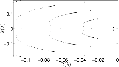
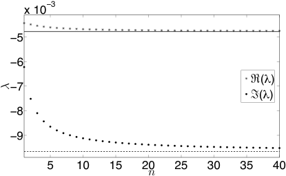
Figure 3: At the steady state 𝐗2superscriptsubscript𝐗2\mathbf{X}_{2}^{*} of the time-rescaled Quartino model (2.30) and the corresponding steady state 𝐘2superscriptsubscript𝐘2\mathbf{Y}_{2}^{*} of the distributed and discrete delay models (2.31) and (2.33) with all parameters from Table 1. (Left): Asterisk for the discrete delay (2.33) characteristic roots that satisfy (3.8), and in gray transitioning to black as n𝑛n is increased from 111 to 404040 characteristic roots for the time-rescaled Quartino model (2.30) and the distributed delay DDE (2.31) which both satisfy (3.11). (Right): Convergence of the real and negative imaginary parts of the rightmost characteristic root, which determines stability as n𝑛n increases.

For the standard parameters, as given in Table 1, we have γ>β𝛾𝛽\gamma>\beta so Theorem 3.1 implies that the neutropenic steady states 𝐗1subscriptsuperscript𝐗1\mathbf{X}^{*}_{1} and 𝐘1subscriptsuperscript𝐘1\mathbf{Y}^{*}_{1} are unstable in all these models. Proving directly that the homeostatic steady states 𝐗2subscriptsuperscript𝐗2\mathbf{X}^{*}_{2} and/or 𝐘2subscriptsuperscript𝐘2\mathbf{Y}^{*}_{2} are stable when γ>β𝛾𝛽\gamma>\beta is difficult, but we can compute the roots of the characteristic equations, and these are shown in Figure 3. We see that the homeostatic steady states are indeed stable when γ>β𝛾𝛽\gamma>\beta. Moreover the characteristic roots for the time-rescaled transit compartment Quartino model converge to the characteristic roots for the discrete delay DDE as n𝑛n increases. Although the steady state is stable for all the models, we see that it becomes less stable as n𝑛n increases, with the real part of the characteristic values tending to increase with n𝑛n. The phenomenon of loss of stability for fixed delay τ𝜏\tau as n𝑛n is increased has long been known, but remains an area of active interest MacDonald89 ; Campbell2009 ; Beretta16 .

In Section 4 we will study how increasing n𝑛n can make the system more susceptible to loss of stability through bifurcations. However, here we point out that the change in stability observed in Theorem 3.1 depending on whether γ>β𝛾𝛽\gamma>\beta or γ<β𝛾𝛽\gamma<\beta is not a bifurcation in the usual sense. When γ=β𝛾𝛽\gamma=\beta the model is degenerate with the progenitor equation reducing to dPdt=0d𝑃d𝑡0\frac{\textrm{d}P}{\textrm{d}t}=0.

In the proof of Theorem 3.1 we made use of the relationships between the different model formulations to greatly simplify the derivation of the stability results. In particular the simpler forms of the characteristic equation for the time-rescaled Quartino (2.30) and DDE models (2.31) and (2.33) makes these much easier to work with. It is nevertheless possible to directly derive stability results for the Quartino model (2.2) at least for the steady state 𝐗1subscriptsuperscript𝐗1\mathbf{X}^{*}_{1}, though the proofs are much more involved. We include those results in Appendix D.2 for completeness.

3.3 Stability of the QSP model of granulopoiesis

Here we perform the linear stability analysis of the steady states of the QSP model defined by the DDE system (2.34), without any exogenous G-CSF, i.e. IG(t)=0subscript𝐼𝐺𝑡0I_{G}(t)=0. Similar to Section 3.2, let 𝐗(t)(Q(t),NR(t),N(t),G1(t),G2(t))𝐗𝑡superscript𝑄𝑡subscript𝑁𝑅𝑡𝑁𝑡subscript𝐺1𝑡subscript𝐺2𝑡\mathbf{X}(t)\coloneqq(Q(t),N_{\!R}(t),N(t),G_{1}(t),G_{2}(t))^{\intercal} be the vector solution of (2.34) and 𝐗σ𝐗(tσ)subscript𝐗𝜎𝐗𝑡𝜎\mathbf{X}_{\sigma}\coloneqq\mathbf{X}(t-\sigma) denote a vector of delayed solutions. Then the DDE system defining the QSP model (2.34) can be rewritten in vector form as

d𝐗dt=𝐅(𝐗,𝐗τQ,𝐗τN,𝐗τNM).𝑑𝐗d𝑡𝐅𝐗subscript𝐗subscript𝜏𝑄subscript𝐗subscript𝜏𝑁subscript𝐗subscript𝜏subscript𝑁𝑀\dfrac{d\mathbf{X}}{\textrm{d}t}=\mathbf{F}(\mathbf{X},\mathbf{X}_{\tau_{Q}},\mathbf{X}_{\tau_{N}},\mathbf{X}_{\tau_{N_{\!M\!}}}). (3.19)

Parameters changes to the model lead to different steady states in equation (3.19). Let the steady state computed at homeostasis be written as 𝐗h(Qh,NRh,Nh,G1h,G2h)superscript𝐗superscript𝑄superscriptsubscript𝑁𝑅superscript𝑁superscriptsubscript𝐺1superscriptsubscript𝐺2\mathbf{X}^{h}\equiv(Q^{h},N_{\!R}^{h},N^{h},G_{1}^{h},G_{2}^{h}), and denote a generic steady state by 𝐗(Q,NR,N,\mathbf{X}^{*}\equiv(Q^{*},N_{\!R}^{*},N^{*},\! G1,G2)G_{1}^{*},G_{2}^{*}).

To linearize (3.19) around a steady state 𝐗superscript𝐗\mathbf{X}^{*} we define the variables τ(t)=τN(t)t𝜏𝑡subscript𝜏𝑁𝑡𝑡\tau(t)=\tau_{N}(t)-t and u=s+τ(t)𝑢𝑠𝜏𝑡u=s+\tau(t) to rewrite the amplification factor (2.39) as

AN(t)=exp[0τNPηNP(G1(uτ(t)))𝑑uγNMτNM(t)].subscript𝐴𝑁𝑡superscriptsubscript0subscript𝜏subscript𝑁𝑃subscript𝜂subscript𝑁𝑃subscript𝐺1𝑢𝜏𝑡differential-d𝑢subscript𝛾subscript𝑁𝑀subscript𝜏subscript𝑁𝑀𝑡A_{N}(t)=\exp{\left[\int_{0}^{\tau_{N_{\!P}}}\eta_{N_{\!P}}(G_{1}(u-\tau(t)))du-\gamma_{N_{\!M}}\tau_{N_{\!M\!}}(t)\right]}. (3.20)

Thus we approximate the amplification factor (3.20) through the linearisation of the proliferation function (2.37) given by

ηNP(G1)=ηNP(G1)+ηNP(G1)(G1G1)+𝒪(|G1G1|2),subscript𝜂subscript𝑁𝑃subscript𝐺1subscript𝜂subscript𝑁𝑃superscriptsubscript𝐺1superscriptsubscript𝜂subscript𝑁𝑃superscriptsubscript𝐺1subscript𝐺1superscriptsubscript𝐺1𝒪superscriptsubscript𝐺1superscriptsubscript𝐺12\eta_{N_{\!P}}(G_{1})=\eta_{N_{\!P}}(G_{1}^{*})+\eta_{N_{\!P}}^{\prime}(G_{1}^{*})(G_{1}-G_{1}^{*})+\mathcal{O}(|G_{1}-G_{1}^{*}|^{2}), (3.21)

where ηNPdηNP/dG1superscriptsubscript𝜂subscript𝑁𝑃𝑑subscript𝜂subscript𝑁𝑃𝑑subscript𝐺1\eta_{N_{\!P}}^{\prime}\equiv d\eta_{N_{\!P}}/dG_{1}. Further, since it does not affect the local stability of the steady state Cooke1996 , we freeze the state-dependent delay at its steady state value

τNM(t)=τNM.subscript𝜏subscript𝑁𝑀𝑡superscriptsubscript𝜏subscript𝑁𝑀\tau_{N_{\!M\!}}(t)=\tau_{N_{\!M\!}}^{*}. (3.22)

Using (3.21) and (3.22) together with the distributed delay variable defined by

G~1(t)0τNPG1(uτ(t))τNP𝑑u,subscript~𝐺1𝑡superscriptsubscript0subscript𝜏subscript𝑁𝑃subscript𝐺1𝑢𝜏𝑡subscript𝜏subscript𝑁𝑃differential-d𝑢\tilde{G}_{1}(t)\coloneqq\int_{0}^{\tau_{N_{\!P}}}\frac{G_{1}(u-\tau(t))}{\tau_{N_{\!P}}}du,

equation (3.20) becomes

A~N(t)=exp[ηNPτNPγNMτNM+ηNP(G1)τNP(G~1(t)G1)].subscript~𝐴𝑁𝑡superscriptsubscript𝜂subscript𝑁𝑃subscript𝜏subscript𝑁𝑃subscript𝛾subscript𝑁𝑀superscriptsubscript𝜏subscript𝑁𝑀superscriptsubscript𝜂subscript𝑁𝑃superscriptsubscript𝐺1subscript𝜏subscript𝑁𝑃subscript~𝐺1𝑡superscriptsubscript𝐺1\tilde{A}_{N}(t)=\exp{\left[\eta_{N_{\!P}}^{*}\tau_{N_{\!P}}-\gamma_{N_{\!M}}\tau_{N_{\!M\!}}^{*}+\eta_{N_{\!P}}^{\prime}(G_{1}^{*})\tau_{N_{\!P}}(\tilde{G}_{1}(t)-G_{1}^{*})\right]}. (3.23)

As a consequence of the approximation in (3.23), we can rewrite (3.19) as

d𝐗dt=𝐟(𝐗,𝐗τQ,𝐗τN,𝐗τNM,𝐗~),𝑑𝐗d𝑡𝐟𝐗subscript𝐗subscript𝜏𝑄subscript𝐗subscript𝜏𝑁subscript𝐗subscript𝜏subscript𝑁𝑀~𝐗\dfrac{d\mathbf{X}}{\textrm{d}t}=\mathbf{f}(\mathbf{X},\mathbf{X}_{\tau_{Q}},\mathbf{X}_{\tau_{N}},\mathbf{X}_{\tau_{N_{\!M\!}}},\tilde{\mathbf{X}}), (3.24)

where

𝐗~(t)0τNP𝐗(uτ(t))τNP𝑑u.~𝐗𝑡superscriptsubscript0subscript𝜏subscript𝑁𝑃𝐗𝑢𝜏𝑡subscript𝜏subscript𝑁𝑃differential-d𝑢\tilde{\mathbf{X}}(t)\coloneqq\int_{0}^{\tau_{N_{\!P}}}\frac{\mathbf{X}(u-\tau(t))}{\tau_{N_{\!P}}}du.

Let 𝐗superscript𝐗\mathbf{X}^{*} be a generic steady state of (3.24), defined by 𝐟(𝐗,𝐗,𝐗,𝐗,𝐗)𝐟superscript𝐗superscript𝐗superscript𝐗superscript𝐗superscript𝐗\mathbf{f}(\mathbf{X}^{*},\mathbf{X}^{*},\mathbf{X}^{*},\mathbf{X}^{*},\mathbf{X}^{*})\! =𝟎absent0=\mathbf{0}. Define the variables 𝐙𝐗𝐗𝐙𝐗superscript𝐗\mathbf{Z}\coloneqq\mathbf{X}-\mathbf{X}^{*}, 𝐙σ𝐗σ𝐗subscript𝐙𝜎subscript𝐗𝜎superscript𝐗\mathbf{Z}_{\sigma}\coloneqq\mathbf{X}_{\sigma}-\mathbf{X}^{*} and 𝐙~𝐗~𝐗~𝐙~𝐗superscript𝐗\tilde{\mathbf{Z}}\coloneqq\tilde{\mathbf{X}}-\mathbf{X}^{*} and denote the linearisation matrices of (3.24) with regards to 𝐗𝐗\mathbf{X}, 𝐗τQsubscript𝐗subscript𝜏𝑄\mathbf{X}_{\tau_{Q}}, 𝐗τNsubscript𝐗subscript𝜏𝑁\mathbf{X}_{\tau_{N}}, 𝐗τNMsubscript𝐗subscript𝜏subscript𝑁𝑀\mathbf{X}_{\tau_{N_{\!M\!}}}, 𝐗τsubscript𝐗𝜏\mathbf{X}_{\tau} and computed at 𝐗superscript𝐗\mathbf{X}^{*}, respectively by 𝔸𝔸\mathds{A}, 𝔹𝔹\mathds{B}, \ldots, 𝔼𝔼\mathds{E}. Linearising (3.5) about 𝐗superscript𝐗\mathbf{X}^{*} and using the variables 𝐙𝐙\mathbf{Z}, 𝐙σsubscript𝐙𝜎\mathbf{Z}_{\sigma} and 𝐙~~𝐙\tilde{\mathbf{Z}} yields

d𝐙dt=𝔸𝐙+𝔹𝐙τQ+𝐙τN+𝔻𝐙τNM+𝔼𝐙~.d𝐙d𝑡𝔸𝐙𝔹subscript𝐙subscript𝜏𝑄subscript𝐙subscript𝜏𝑁𝔻subscript𝐙subscript𝜏subscript𝑁𝑀𝔼~𝐙\frac{\textrm{d}\mathbf{Z}}{\textrm{d}t}=\mathds{A}\mathbf{Z}+\mathds{B}\mathbf{Z}_{\tau_{Q}}+\mathds{C}\mathbf{Z}_{\tau_{N}}+\mathds{D}\mathbf{Z}_{\tau_{N_{\!M\!}}}+\mathds{E}\tilde{\mathbf{Z}}. (3.25)

The linearisation matrices 𝔸𝔸\mathds{A}, 𝔹𝔹\mathds{B}, \ldots, 𝔼𝔼\mathds{E} from (3.25) are computed in Appendix D.4. Seeking a nontrivial exponential solution 𝐙(t)=𝐂eλt𝐙𝑡𝐂superscript𝑒𝜆𝑡\mathbf{Z}(t)=\mathbf{C}e^{\lambda t} for equation (3.25), with constant 𝐂5𝐂superscript5\mathbf{C}\in\mathds{R}^{5} and λ𝜆\lambda\in\mathbb{C}, we obtain the characteristic equation

det(λ𝕀𝔸eλτQ𝔹eλτNeλτNM𝔻f(λ)𝔼)=0,𝜆𝕀𝔸superscript𝑒𝜆subscript𝜏𝑄𝔹superscript𝑒𝜆superscriptsubscript𝜏𝑁superscript𝑒𝜆superscriptsubscript𝜏subscript𝑁𝑀𝔻𝑓𝜆𝔼0\det(\lambda\mathds{I}-\mathds{A}-e^{-\lambda\tau_{Q}}\mathds{B}-e^{-\lambda\tau_{N}^{*}}\mathds{C}-e^{-\lambda\tau_{N_{\!M\!}}^{*}}\mathds{D}-f(\lambda)\mathds{E})=0, (3.26)

where 𝕀𝕀\mathds{I} is the identity matrix and

f(λ)(eλτNP1)λτNPeλτN=eλτNMeλτNλτNP.𝑓𝜆superscript𝑒𝜆subscript𝜏subscript𝑁𝑃1𝜆subscript𝜏subscript𝑁𝑃superscript𝑒𝜆superscriptsubscript𝜏𝑁superscript𝑒𝜆superscriptsubscript𝜏subscript𝑁𝑀superscript𝑒𝜆superscriptsubscript𝜏𝑁𝜆subscript𝜏subscript𝑁𝑃f(\lambda)\coloneqq\frac{(e^{\lambda\tau_{N_{\!P}}}-1)}{\lambda\tau_{N_{\!P}}e^{\lambda\tau_{N}^{*}}}=\frac{e^{-\lambda\tau_{N_{\!M\!}}^{*}}-e^{-\lambda\tau_{N}^{*}}}{\lambda\tau_{N_{\!P}}}.

For λ=reiθ𝜆𝑟superscript𝑒𝑖𝜃\lambda=re^{i\theta}, with r,θ𝑟𝜃r,\theta\in\mathds{R}, we have limr0f(reiθ)=1subscript𝑟0𝑓𝑟superscript𝑒𝑖𝜃1\lim_{r\rightarrow 0}f(re^{i\theta})=1. We rearrange equation (3.26) in the form det(𝔽)=0𝔽0\det(\mathds{F})=0. To calculate the matrix 𝔽𝔽\mathds{F}, with terms Fijsubscript𝐹𝑖𝑗F_{ij} for i,j={1,2,,5}𝑖𝑗125i,j=\{1,2,\ldots,5\}, note that some terms of the linearisation matrices are symmetric while others are antisymmetric, namely A43=A42subscript𝐴43subscript𝐴42A_{43}=A_{42}, A52=A42subscript𝐴52subscript𝐴42A_{52}=-A_{42}, A53=A42subscript𝐴53subscript𝐴42A_{53}=-A_{42}, A35=A25subscript𝐴35subscript𝐴25A_{35}=-A_{25}, and D24=A24subscript𝐷24subscript𝐴24D_{24}=-A_{24} (see Appendix D.4). Using this fact, we can then compute the terms

F11(λ)=A11λ+B11eλτQ,Fii(λ)=Aiiλfori=2,3,4,5,formulae-sequenceformulae-sequencesubscript𝐹11𝜆subscript𝐴11𝜆subscript𝐵11superscript𝑒𝜆subscript𝜏𝑄subscript𝐹𝑖𝑖𝜆subscript𝐴𝑖𝑖𝜆for𝑖2345F_{11}(\lambda)=A_{11}-\lambda+B_{11}e^{-\lambda\tau_{Q}},\ F_{ii}(\lambda)=A_{ii}-\lambda\ \mbox{for}\ i=2,3,4,5,
F21(λ)=C21eλτN,F24(λ)=A24(1eλτNM)+C24eλτN+E24f(λ),formulae-sequencesubscript𝐹21𝜆subscript𝐶21superscript𝑒𝜆superscriptsubscript𝜏𝑁subscript𝐹24𝜆subscript𝐴241superscript𝑒𝜆superscriptsubscript𝜏subscript𝑁𝑀subscript𝐶24superscript𝑒𝜆superscriptsubscript𝜏𝑁subscript𝐸24𝑓𝜆F_{21}(\lambda)=C_{21}e^{-\lambda\tau_{N}^{*}},\quad F_{24}(\lambda)=A_{24}(1-e^{-\lambda\tau_{N_{\!M\!}}^{*}})+C_{24}e^{-\lambda\tau_{N}^{*}}+E_{24}f(\lambda),

and write the matrix 𝔽𝔽\mathds{F} as

𝔽=[F11(λ)00A120F21(λ)F22(λ)A23F24(λ)A250A32F33(λ)0A250A42A42F44(λ)A450A42A42A54F55(λ)].𝔽matrixsubscript𝐹11𝜆00subscript𝐴120subscript𝐹21𝜆subscript𝐹22𝜆subscript𝐴23subscript𝐹24𝜆subscript𝐴250subscript𝐴32subscript𝐹33𝜆0subscript𝐴250subscript𝐴42subscript𝐴42subscript𝐹44𝜆subscript𝐴450subscript𝐴42subscript𝐴42subscript𝐴54subscript𝐹55𝜆\mathds{F}=\begin{bmatrix}F_{11}(\lambda)&0&0&A_{12}&0\\ F_{21}(\lambda)&F_{22}(\lambda)&A_{23}&F_{24}(\lambda)&A_{25}\\ 0&A_{32}&F_{33}(\lambda)&0&-A_{25}\\ 0&A_{42}&A_{42}&F_{44}(\lambda)&A_{45}\\ 0&-A_{42}&-A_{42}&A_{54}&F_{55}(\lambda)\\ \end{bmatrix}.

Defining the constants

K1=A45A54,K2=A42A25,K3=A42A25A54,formulae-sequencesubscript𝐾1subscript𝐴45subscript𝐴54formulae-sequencesubscript𝐾2subscript𝐴42subscript𝐴25subscript𝐾3subscript𝐴42subscript𝐴25subscript𝐴54\displaystyle K_{1}=-A_{45}A_{54},\qquad K_{2}=-A_{42}A_{25},\qquad K_{3}=-A_{42}A_{25}A_{54},
K4=A42A25,K5=A32A23,K6=(A23A32)A25A42,formulae-sequencesubscript𝐾4subscript𝐴42subscript𝐴25formulae-sequencesubscript𝐾5subscript𝐴32subscript𝐴23subscript𝐾6subscript𝐴23subscript𝐴32subscript𝐴25subscript𝐴42\displaystyle K_{4}=A_{42}A_{25},\qquad K_{5}=-A_{32}A_{23},\qquad K_{6}=(A_{23}-A_{32})A_{25}A_{42},
K7=A42A25A54,K8=[A32(A23A45A42A25)+A42A23A25]A54,formulae-sequencesubscript𝐾7subscript𝐴42subscript𝐴25subscript𝐴54subscript𝐾8delimited-[]subscript𝐴32subscript𝐴23subscript𝐴45subscript𝐴42subscript𝐴25subscript𝐴42subscript𝐴23subscript𝐴25subscript𝐴54\displaystyle K_{7}=A_{42}A_{25}A_{54},\qquad K_{8}=[A_{32}(A_{23}A_{45}-A_{42}A_{25})+A_{42}A_{23}A_{25}]A_{54},
K9=A42A45,K10=A32A42,K11=A32A42A45,formulae-sequencesubscript𝐾9subscript𝐴42subscript𝐴45formulae-sequencesubscript𝐾10subscript𝐴32subscript𝐴42subscript𝐾11subscript𝐴32subscript𝐴42subscript𝐴45\displaystyle K_{9}=-A_{42}A_{45},\qquad K_{10}=A_{32}A_{42},\qquad K_{11}=A_{32}A_{42}A_{45},

and the functions

ρ(λ)𝜌𝜆\displaystyle\rho(\lambda) =\displaystyle= F22(λ)[F33(λ)F44(λ)F55(λ)+K1F33(λ)+K2F44(λ)+K3]+limit-fromsubscript𝐹22𝜆delimited-[]subscript𝐹33𝜆subscript𝐹44𝜆subscript𝐹55𝜆subscript𝐾1subscript𝐹33𝜆subscript𝐾2subscript𝐹44𝜆subscript𝐾3\displaystyle F_{22}(\lambda)[F_{33}(\lambda)F_{44}(\lambda)F_{55}(\lambda)+K_{1}F_{33}(\lambda)+K_{2}F_{44}(\lambda)+K_{3}]+
F44(λ)[K4F33(λ)+K5F55(λ)+K6]+K7F33(λ)+K8+subscript𝐹44𝜆delimited-[]subscript𝐾4subscript𝐹33𝜆subscript𝐾5subscript𝐹55𝜆subscript𝐾6subscript𝐾7subscript𝐹33𝜆limit-fromsubscript𝐾8\displaystyle F_{44}(\lambda)[K_{4}F_{33}(\lambda)+K_{5}F_{55}(\lambda)+K_{6}]+K_{7}F_{33}(\lambda)+K_{8}+
F24(λ)[K9F33(λ)+K10F55(λ)A42F33(λ)F55(λ)+K11],subscript𝐹24𝜆delimited-[]subscript𝐾9subscript𝐹33𝜆subscript𝐾10subscript𝐹55𝜆subscript𝐴42subscript𝐹33𝜆subscript𝐹55𝜆subscript𝐾11\displaystyle F_{24}(\lambda)[K_{9}F_{33}(\lambda)+K_{10}F_{55}(\lambda)-A_{42}F_{33}(\lambda)F_{55}(\lambda)+K_{11}],
ψ(λ)=F21(λ)[A42F33(λ)F55(λ)K9F33K10F55(λ)K11]A12,𝜓𝜆subscript𝐹21𝜆delimited-[]subscript𝐴42subscript𝐹33𝜆subscript𝐹55𝜆subscript𝐾9subscript𝐹33subscript𝐾10subscript𝐹55𝜆subscript𝐾11subscript𝐴12\psi(\lambda)=F_{21}(\lambda)[A_{42}F_{33}(\lambda)F_{55}(\lambda)-K_{9}F_{33}-K_{10}F_{55}(\lambda)-K_{11}]A_{12},

the characteristic equation det(𝔽)=0𝔽0\det(\mathds{F})=0 becomes

F11(λ)ρ(λ)+ψ(λ)=0.subscript𝐹11𝜆𝜌𝜆𝜓𝜆0F_{11}(\lambda)\rho(\lambda)+\psi(\lambda)=0. (3.27)
Refer to caption
Figure 4: Roots of the characteristic equation (3.27) of the QSP granulopoiesis model (2.34) evaluated at the homeostasis steady state 𝐗hsuperscript𝐗\mathbf{X}^{h} all have negative real part in the complex plane.

The solutions λ𝜆\lambda\in\mathbb{C} to (3.27), the characteristic roots, determine the stability of the steady state 𝐗superscript𝐗\mathbf{X}^{*} from (3.19)/(3.25). To evaluate the stability numerically, we write λ=σ+iω𝜆𝜎𝑖𝜔\lambda=\sigma+i\omega, with σ𝜎\sigma\in\mathds{R} and ω𝜔\omega\in\mathds{R}, and then compute the roots of (3.27) in the (σ,ω)𝜎𝜔(\sigma,\omega)-plane using the Matlab subroutine fsolve Mathworks . As illustrated in Figure 4, at homeostasis all the characteristic roots λ𝜆\lambda have negative real part, and so the homeostatic steady state 𝐗h=(Qh,NRh,Nh,G1h,G2h)superscript𝐗superscript𝑄superscriptsubscript𝑁𝑅superscript𝑁superscriptsubscript𝐺1superscriptsubscript𝐺2\mathbf{X}^{h}=(Q^{h},N_{\!R}^{h},N^{h},G_{1}^{h},G_{2}^{h}), defined by 𝐅(𝐗h,𝐗h,𝐗h,𝐗h)=𝟎𝐅superscript𝐗superscript𝐗superscript𝐗superscript𝐗0\mathbf{F}(\mathbf{X}^{h},\mathbf{X}^{h},\mathbf{X}^{h},\mathbf{X}^{h})=\mathbf{0} in (3.19) is locally asymptotically stable.

4 Bifurcation studies

Bifurcation analysis, or the study of the qualitative changes to the behaviour of a system given a change to parameter values, is a fundamental dynamical systems concept Meiss2007 . Accordingly, studying bifurcation points can be a powerful tool in the life sciences to shed light on underlying parameter relationships and better understand the robustness of a system with regards to stability.

Historically, bifurcation analysis has been applied to study hematological pathologies and has provided valuable insight into the origins of disorders like cyclic neutropenia, a disease associated with dangerously low neutrophil counts and mouth blistering Dale2015 where a patient’s ANCs oscillate with a period of around 21 days. These oscillations have been shown to correspond to a periodic orbit that appears through a loss of stability after the system undergoes a Hopf bifurcation Colijn:2 ; Foley2009b . In the following sections, we perform bifurcation analyses on the equivalent forms of the Quartino endogenous G-CSF model and the QSP granulopoiesis model (2.34) to ascertain how changing parameter values modify the stability of each system, giving insight into the potential effects of PK variability on a physiological system and helping to understand pathophysiology of diseases.

4.1 Bifurcation in the equivalent expressions of the Quartino endogenous G-CSF model

We begin by investigating whether parameter changes in the equivalent expressions of the Quartino endogenous G-CSF model can lead their steady states 𝐗2subscriptsuperscript𝐗2\mathbf{X}^{*}_{2} and 𝐘2subscriptsuperscript𝐘2\mathbf{Y}^{*}_{2} given by (3.15) and (3.17), respectively, to lose stability. For this, we let λ=σ+iω𝜆𝜎𝑖𝜔\lambda=\sigma+i\omega, where σ𝜎\sigma\in\mathds{R} and ω𝜔\omega\in\mathds{R}, and computed the roots of the characteristic equations (D.6), (3.8) and (3.11) in the (σ,ω)𝜎𝜔(\sigma,\omega)-plane using the Matlab subroutines roots and fsolve Mathworks .

We saw in Section 3.2 that the homeostasis steady states 𝐗2subscriptsuperscript𝐗2\mathbf{X}^{*}_{2} and 𝐘2subscriptsuperscript𝐘2\mathbf{Y}^{*}_{2} are locally asymptotically stable in all the versions of the Quartino model that we consider, and that the models are degenerate when β=γ𝛽𝛾\beta=\gamma, consequently here we will study the bifurcations that occur as parameters are varied from their homeostasis values with γ>β𝛾𝛽\gamma>\beta.

We begin by studying the Quartino model (2.2) starting from parameters used in Quartino2014 , so n=4𝑛4n=4, a=ktr𝑎subscript𝑘𝑡𝑟a=k_{tr} and all the other parameters as in Table 1. We observed that changes to γ𝛾\gamma, the parameter relating the feedback of circulating G-CSF concentrations on the proliferating pool, and a𝑎a, the transit rate between maturation compartments, can lead to a loss of stability giving rise to a periodic orbit via a Hopf bifurcation. Table 2 summarises the parameter pair values (γ,a)𝛾𝑎(\gamma,a) necessary to induce such a loss in stability in 𝐗2subscriptsuperscript𝐗2\mathbf{X}^{*}_{2}, and the resulting period of the emerging periodic orbits.

If we let γ𝛾\gamma be the bifurcation parameter and keep the remaining parameters at their homeostasis values (see Table 1), there is a Hopf bifurcation point at γ=0.86766𝛾0.86766\gamma=0.86766. We verified numerically that 𝐗2subscriptsuperscript𝐗2\mathbf{X}^{*}_{2} is locally asymptotically stable for β<γ<0.86766𝛽𝛾0.86766\beta<\gamma<0.86766 and unstable if γ>0.86766𝛾0.86766\gamma>0.86766. Of particular interest, as reflected in the bolded row of Table 2, we found a periodic orbit characteristic of cyclical neutropenia Dale2015 . Using the relation a=n/a=n/MMT with n=4𝑛4n=4 gives the value MMT=123.33hoursabsent123.33hours=123.33\,\text{hours}, which is close to the mean maturation time of 133 hours for a patient under chemotherapy treatment reported by Quartino Quartino2014 .

In Figure 5 (left) we show the Hopf bifurcation curve for 𝐗2subscriptsuperscript𝐗2\mathbf{X}^{*}_{2} on parameter space (a,γ)𝑎𝛾(a,\gamma) for the Quartino model (2.2). The steady state is stable in the region below the Hopf curve and unstable otherwise. In Figure 5 (right) we see that increasing γ𝛾\gamma for small values of the transit rate parameter n𝑛n lead to solutions with long period.

Refer to caption
Refer to caption
Figure 5: Hopf bifurcation curve for 𝐗2subscriptsuperscript𝐗2\mathbf{X}^{*}_{2} on parameter space (a,γ)𝑎𝛾(a,\gamma) (Left) and the respective period (in days) as function of a𝑎a (Right) for the Quartino model (2.2). The remaining parameters are as in Table 1 and the diamond dot correspond to a𝑎a at its homeostasis value 0.03759 hours-1.
γ𝛾\gamma (-) a𝑎a (hours-1) τ𝜏\tau (hours) Period (days)
0.87851 0.03831 104.4 18.0018.0018.00
0.86766 0.03759 106.41 18.3218.3218.32
0.789110.78911\mathbf{0.78911} 0.032430.03243\mathbf{0.03243} 123.33123.33\mathbf{123.33} 21.021.0\mathbf{21.0}
Table 2: Hopf bifurcation points for varying γ𝛾\gamma, a𝑎a, and τ𝜏\tau for 𝐗2subscriptsuperscript𝐗2\mathbf{X}^{*}_{2} computed as in Figure 5, Values highlighted in bold correspond to periods characteristic of patients with cyclic neutropenia.

In the same vein, we also computed bifurcation points for the equilibrium 𝐗2subscriptsuperscript𝐗2\mathbf{X}^{*}_{2} of distributed DDE model (2.31) using the characteristic equation (3.11) with n=4𝑛4n=4. As expected, given that the this model is simply a time-rescaling of the Quartino model (2.2) we obtain the same bifurcation points shown in Table 2.

γ𝛾\gamma (-) n𝑛n (-) Period (days)
4.61186 1 7.767
1.69292 1.5 13.53
1.21571 2 15.95
0.90252 3.5 18.08
0.867660.86766\mathbf{0.86766} 𝟒4\mathbf{4} 18.3218.32\mathbf{18.32}
0.75312 10 18.98
0.72367 20 19.08
0.71461 30 19.09
0.71021 40 19.10
0.69754 \infty 19.11
Table 3: Hopf bifurcation points for varying γ𝛾\gamma and n𝑛n for 𝐘2subscriptsuperscript𝐘2\mathbf{Y}^{*}_{2} computed as in Table 6 but considering the characteristic equation of the distributed DDE model (3.11). The other parameters were fixed at their homeostasis values given in Table 1. The last row corresponds to the discrete delay case.

In Figure 6 (left) we show the Hopf bifurcation curve for 𝐘2subscriptsuperscript𝐘2\mathbf{Y}^{*}_{2} on parameter space (n,γ)𝑛𝛾(n,\gamma) for the distributed DDE model (2.31). The steady state is stable in the region below the Hopf curve and unstable otherwise. Increasing n𝑛n lead to γ𝛾\gamma and the period of the Hopf bifurcation converge to the bifurcation point of the discrete DDE model (2.33) shown in the bolded row of Table 4.
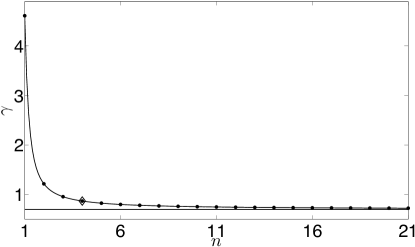
Refer to caption
Refer to caption
Figure 6: Hopf bifurcation curve for 𝐘2subscriptsuperscript𝐘2\mathbf{Y}^{*}_{2} on parameter space (n,γ)𝑛𝛾(n,\gamma) (Left) and the respective period (in days) as function of n𝑛n (Right) for the distributed DDE model (2.31). The other parameters are as in Table 1 and the diamond dot correspond to n𝑛n at its homeostasis value 4. The straight lines correspond to the bifurcation point γ𝛾\gamma and its respective period for the discrete DDE model with other parameters at their homeostasis values.

Table 4 reports bifurcation points computed for the steady state 𝐘2subscriptsuperscript𝐘2\mathbf{Y}^{*}_{2} of the discrete DDE model (2.33) using the characteristic equation (3.8). Comparing the second rows of Tables 2 and 4, we note that the region of stability for the discrete DDE model β<γ<0.69754𝛽𝛾0.69754\beta<\gamma<0.69754 is smaller than that of the distributed DDE with n=4𝑛4n=4, and of the equivalent ODE Quartino model β<γ<0.86766𝛽𝛾0.86766\beta<\gamma<0.86766. Furthermore, we verified that in the limit n𝑛n\to\infty with a=n/τ𝑎𝑛𝜏a=n/\tau or a=(n+1)/τ𝑎𝑛1𝜏a=(n+1)/\tau and holding τ𝜏\tau fixed, the characteristic roots of the distributed DDE model (3.11) converge to the roots of the discrete DDE model (3.8) since (3.11) approaches to (3.8) when n𝑛n\to\infty.

γ𝛾\gamma (-) τ𝜏\tau (hours) Period (days)
0.72631 99.8 18.00
0.697540.69754\mathbf{0.69754} 106.41106.41\mathbf{106.41} 19.1119.11\mathbf{19.11}
0.65534 117.75 21.00
Table 4: Hopf bifurcation points for varying γ𝛾\gamma and τ𝜏\tau for 𝐘2subscriptsuperscript𝐘2\mathbf{Y}^{*}_{2} computed as in Table 6 but considering the characteristic equation of the discrete DDE model (3.8). The other parameters were fixed at their homeostasis values given in Table 1.

In Figure 7 (left) we show the Hopf bifurcation curve for 𝐘2subscriptsuperscript𝐘2\mathbf{Y}^{*}_{2} on parameter space (τ,γ)𝜏𝛾(\tau,\gamma) for the discrete DDE model (2.33). The steady state is stable in the region below the Hopf curve and unstable otherwise. In Figure 7 (right) we see that there is an approximate linear relation between the period of the limit cycles and the mean value of the distributed delay τ𝜏\tau for along all values of γ𝛾\gamma.

Refer to caption
Refer to caption
Figure 7: Hopf bifurcation curve for 𝐘2subscriptsuperscript𝐘2\mathbf{Y}^{*}_{2} on parameter space (τ,γ)𝜏𝛾(\tau,\gamma) (Left) and the respective period (in days) as function of τ𝜏\tau (Right) for the discrete DDE model (2.33). Squares represent integer numbers n𝑛n. The remaining parameters are as in Table 1 and the diamond dot correspond to τ𝜏\tau at its homeostasis value 106.41 hours.

4.2 Bifurcations in the QSP model of granulopoiesis

We also studied whether parameter changes can lead the steady state 𝐗superscript𝐗\mathbf{X}^{*} of system (2.34) to lose stability. We observed that changes in parameters related to proliferation and maturation lead to a loss of stability via a Hopf bifurcation, as reflected in Table 5. Inversely, we further verified the stability of the steady state when the half-maximal neutrophil proliferation constant satisfies bNP[bNP×103,bNP×103]subscript𝑏subscript𝑁𝑃subscript𝑏subscript𝑁𝑃superscript103subscript𝑏subscript𝑁𝑃superscript103b_{N_{\!P}}\in[b_{N_{\!P}}\times{10}^{-3},b_{N_{\!P}}\times{10}^{3}], the rate of maturing neutrophil death satisfies γNM[γNM×102,γNM×102]subscript𝛾subscript𝑁𝑀subscript𝛾subscript𝑁𝑀superscript102subscript𝛾subscript𝑁𝑀superscript102\gamma_{N_{\!M}}\in[\gamma_{N_{\!M}}\times{10}^{-2},\gamma_{N_{\!M}}\times{10}^{2}], and the neutrophil apoptosis rate in the bone marrow reservoir satisfies γNR[γNR×102,γNR×102]subscript𝛾subscript𝑁𝑅subscript𝛾subscript𝑁𝑅superscript102subscript𝛾subscript𝑁𝑅superscript102\gamma_{N_{\!R}}\in[\gamma_{N_{\!R}}\times{10}^{-2},\gamma_{N_{\!R}}\times{10}^{2}].

We further investigated whether varying pairs of parameters in tandem could lead the steady state to lose stability via a Hopf bifurcation, as reflected in Table 6. An additional Hopf bifurcation point leading to an orbit of period of 20.9420.9420.94 days was observed by changing four parameters simultaneously: ηNPh=1.7days1superscriptsubscript𝜂subscript𝑁𝑃1.7superscriptdays1\eta_{N_{\!P}}^{h}=1.7\,\text{days}^{-1}; bNP=2.0subscript𝑏subscript𝑁𝑃2.0b_{N_{\!P}}=2.0 ng/mL; ηNPmin=1.3days1superscriptsubscript𝜂subscript𝑁𝑃min1.3superscriptdays1\eta_{N_{\!P}}^{\textit{min}}=1.3\,\text{days}^{-1}; and τNP=6.1dayssubscript𝜏subscript𝑁𝑃6.1days\tau_{N_{\!P}}=6.1\,\text{days}.

Parameter (units) Homeostasis Value Hopf Bifurcation Period (days)
γQsubscript𝛾𝑄\gamma_{Q} (days-1) 0.10.10.1 0.227910.227910.22791 36.6936.6936.69
ηNPhsuperscriptsubscript𝜂subscript𝑁𝑃\eta_{N_{\!P}}^{h} (days-1) 1.66471.66471.6647 7.47.47.4 60.3160.3160.31
ηNPminsuperscriptsubscript𝜂subscript𝑁𝑃𝑚𝑖𝑛\eta_{N_{\!P}}^{min} (days-1) 1.40601.40601.4060 0.810.810.81 25.8625.8625.86
Vmaxsubscript𝑉𝑚𝑎𝑥V_{max} (-) 7.86697.86697.8669 939393 5.205.205.20
bVsubscript𝑏𝑉b_{V} (ng/mL) 0.246100.246100.24610 0.01840.01840.0184 5.205.205.20
Table 5: For each line the Hopf bifurcation point were computed changing the respective parameter and following the solution λ𝜆\lambda of Eq. (3.27) in the (σ,ω)𝜎𝜔(\sigma,\omega)-plane numerically, the period was estimated by 2π/ω2𝜋𝜔2\pi/\omega and the parameters values at homeostasis were obtained from Craig2016c .
Parameters  (units) Hopf Bifurcation Period (days)
(Vmax,bV)subscript𝑉𝑚𝑎𝑥subscript𝑏𝑉(V_{max},b_{V})  (-,ng/mL) (30,7.8)307.8(30,7.8) 5.205.205.20
(Vmax,bV)subscript𝑉𝑚𝑎𝑥subscript𝑏𝑉(V_{max},b_{V})  (-,ng/mL) (61,16.1)6116.1(61,16.1) 5.205.205.20
(bNP,ηNPmin)subscript𝑏subscript𝑁𝑃superscriptsubscript𝜂subscript𝑁𝑃𝑚𝑖𝑛(b_{N_{\!P}},\eta_{N_{\!P}}^{min})  (ng/mL,days-1) (0.065,1.1)0.0651.1(0.065,1.1) 25.8625.8625.86
(ηNPh,ηNPmin)superscriptsubscript𝜂subscript𝑁𝑃superscriptsubscript𝜂subscript𝑁𝑃min(\eta_{N_{\!P}}^{h},\eta_{N_{\!P}}^{\textit{min}})  (days-1,ng/mL) (2,1.1)21.1(2,1.1) 32.5832.5832.58
Table 6: For each line the Hopf bifurcation point were computed changing the respective pair of parameters and following the solution λ𝜆\lambda of Eq. (3.27) in the (σ,ω)𝜎𝜔(\sigma,\omega)-plane numerically, the period was estimated by 2π/ω2𝜋𝜔2\pi/\omega and the parameters values at homeostasis were obtained from Craig2016c .

5 The impact of stability and bifurcations on PK/PD considerations

In the PK/PD context, sensitivity analysis is frequently applied to investigate the impact of parameters variability on the system’s output. There the goal is to understand how predictions (outputs) change given changes to initial values (inputs). Still, when evaluating treatments, one may wonder how small changes to parameters affect the qualitative (e.g. existence and stability of equilibria, etc.) behaviour of the model. For example, if we have a priori information about a PK parameter’s variability and this parameter helps determine the model’s stability, bifurcation analysis can help to assess whether small changes within the range of the measured variability can bring about serious unintended shifts in the physiological system. Put another way, how are parameters changing when the system shifts stability or becomes unstable? Bifurcation analysis is rarely used in conventional PK/PD analyses, however the study of qualitative model behaviour is becoming increasingly recognised as an important tool for drug development Bakshi2016 ; Ghosh2013 . The potential impact of variability in PK parameters on the dynamics of the governing equations, which correspond to the PD aspects, is multifaceted. Within pharmacometrics, various situations must therefore be considered when assessing which (and how) parameters are susceptible to generating bifurcations when their values change.

In the simplest case, for physiological or drug parameters not influenced by drug concentration, no bifurcation can be generated through any PK variability. Examples of such parameters could include the maximal achievable response in an Emax model or a zero-order endogenous production rate. In that vein, we observe that in the Quartino model, the bifurcation point for γ𝛾\gamma is not likely to be reached by realistic variations in G-CSF concentrations.

More familiar to the pharmacometrician is the case where different parameters values associated with specific cohorts and/or patient subpopulations correspond to individual states in the dynamical system. Here bifurcation analysis is analogous to Population-PK (Pop-PK) covariate analysis techniques used to separate and determine Pop-PK models for each subgroup. From this covariate analysis, one infers that for each state, there is a particular PK/PD model for which the (between subject) variability has been explained. Accordingly, Pop-PK covariate studies examine the impact of between subject variability is readily accounted for during the process of building a Pop-PK model. In the same way, bifurcation analysis of mathematical models helps to ascertain how changes to (variability in) model parameters affect the stable state. Of note, in the most complex case, where the parameters of a dynamical system are affected by PKs (which can also vary during therapy), within subject variability in PK is an important factor in determining model stability and a case-by-case model analysis must be carried out.

The impact of interindividual variability (IIV) is also an open question when considering the time-rescaled Quartino (2.30) and discrete delay (2.33) models. Since the discrete delay model is the equivalent to taking n𝑛n to infinity in (2.30), we investigated whether there would be altered behaviour due to IIV with increases in n𝑛n. We began by generating 30 virtual patients using the docetaxel Pop-PK model of Bruno Bruno1996 and set Edrug=SlopeCdocsubscript𝐶docC_{\text{doc}}, as in Quartino2014 , where Cdocsubscript𝐶docC_{\text{doc}} is the concentration of docetaxel in the central compartment. Using the same individual patient values for the generalised and time-rescaled Quartino models, we verified that solutions to (2.2) were identical as the solutions to (2.30) when the latter were rescaled according to (2.29) (not shown). We proceeded to compare the full Pop-PK predictions of (2.2) for these 30 virtual patients when n=4𝑛4n=4 and n=10𝑛10n=10. In Figure 8, increases to n𝑛n are not significantly affected by the inclusion of IIV, though increases to n𝑛n decidedly impact on the distribution of solutions. Given these results and to better visualise the impact of increasing n𝑛n, we then compared the predictions of (2.2) to (2.33) (the case of infinite n𝑛n) using only the typical parameter estimates. As seen in Figure 9, in the limit n𝑛n\to\infty, solutions to the generalised Quartino model (and equivalently, the time-rescaled Quartino and distributed delay models) converge to that of the discrete delay. Further, as n𝑛n increases, so too does the dimension of the resulting ODE system for (2.2), which is not the case for the 3 equations of (2.33), thereby encouraging the use of a delay model to speed up simulation time. It should be noted that in all simulations described in this section, due to the misspecification of MMT as MMT=(n+1)/ktr𝑛1subscript𝑘𝑡𝑟(n+1)/k_{tr}, to compare directly with the results of Quartino2014 ktr=kPsubscript𝑘𝑡𝑟subscript𝑘Pk_{tr}=k_{\textit{\tiny P}} were fixed to the value in Table 1, MMT was taken to be 133 hours, and τ𝜏\tau was recalculate as τ=(4/5)MMT𝜏45MMT\tau=(4/5)\text{MMT}, with a=n/τ𝑎𝑛𝜏a=n/\tau.

Refer to caption

P(t)𝑃𝑡P(t)

Days

(a) n=4𝑛4n=4
Refer to caption

P(t)𝑃𝑡P(t)

Days

(b) n=10𝑛10n=10
Refer to caption

Nt)Nt)

Days

(c) n=4𝑛4n=4
Refer to caption

N(t)𝑁𝑡N(t)

Days

(d) n=10𝑛10n=10
Refer to caption

G(t)𝐺𝑡G(t)

Days

(e) n=4𝑛4n=4
Refer to caption

G(t)𝐺𝑡G(t)

Days

(f) n=10𝑛10n=10
Figure 8: Impact of IIV on the Quartino model (2.2) and its equivalent forms (2.30) and (2.31) for two different values of n𝑛n. PopPK parameters for 30 virtual patients were generated following Bruno1996 and used as inputs to (2.2). Solid blue lines: individual predictions; black dotted-dashed lines: 10th and 90th percentiles of predictions; red dashed lines: median prediction.
Refer to caption

N(t)𝑁𝑡N(t)

Days

(a) Neutrophils
Refer to caption

G(t)𝐺𝑡G(t)

Days

(b) G-CSF
Figure 9: Neutrophil and G-CSF concentrations from the generalised Quartino model (2.2) and the equivalent time-rescaled discrete delay model (2.33) for increasing values of n𝑛n. Since the discrete delay model (2.33) is expressed in the time-rescaled t^(t)^𝑡𝑡\hat{t}(t), we inverted (2.29)italic-(2.29italic-)\eqref{lctsd1} and mapped the simulated solution back to t𝑡t to directly compare to (2.2). Dashed line: solution of discrete delay.

The analysis and results of Section 3.3 indicate the interest of performing stability and bifurcation studies in the pharmaceutical sciences setting. Through sensitivity analysis, we have previously concluded that models constructed from first-principles, such as (2.34), are robust to PKs by “sufficiently” accounting for the system’s physiological mechanisms Craig2016 . Thus average PK parameters without reference to the full Pop-PK model are reliably predictive of the behaviour of such physiological models. Here we extend our previous work to study how PK variability (variations in G-CSF concentrations) affect the stable states of the PD (physiological) system.

The granulopoietic system is indeed very robust around homeostatic parameter values. An increase in G-CSF concentrations corresponds to a decrease in the value of γQsubscript𝛾𝑄\gamma_{Q}, and, from Table 5, destabilisation of this equilibrium can only occur when γq>γQhsubscript𝛾𝑞subscriptsuperscript𝛾𝑄\gamma_{q}>\gamma^{h}_{Q}, and thus such changes preserve homeostasis. With regard to changes in the proliferative progenitor compartment, either by variations in the parameters ηNPhsubscriptsuperscript𝜂subscript𝑁𝑃\eta^{h}_{N_{P}} or bvsubscript𝑏𝑣b_{v}, physiologically realistic scenarios preclude reaching the bifurcation values: for example, in the case of ηNPhsubscriptsuperscript𝜂subscript𝑁𝑃\eta^{h}_{N_{P}}, artificial removal of G-CSF from the body would be required.

6 Discussion

Mathematical pharmacology, defined as the study of mathematical approaches to pharmacological processes, is increasingly recognised as a quantitative methodology critical to understanding pharmaceutical treatments and their efficacy while simultaneously raising compelling mathematical problems vanderGraaf2016 . Using granulopoiesis as a backdrop, in the present paper we have examined the connections between the familiar PK/PD model formalism originally proposed by Friberg Friberg2002 and adapted by Quartino Quartino2014 and a discrete delay model of neutrophil production, connected via a distributed delay model. Crucially, we have shown how the stability of each model can be studied straightforwardly via this latter distributed delay model, underlining the advantage of being able to transfer between these equivalent expressions and motivating the present analysis. We examined the impact of the inclusion of IIV on the solutions to each of the models, and determined that variations are driven through increases to n𝑛n rather than the presence of variability; as n𝑛n\to\infty, solutions of the generalised (time-rescaled) Quartino transit compartment model converge to that of the time-rescaled discrete DDE model. Last, using our previously published QSP model of the negative feedback relationship between granulopoiesis and G-CSF, we have identified several Hopf bifurcations through bifurcation analysis, a technique not commonly applied in the classical PK/PD analyses, and reviewed the impact the interpretation of such bifurcations can have on our understanding of pharmacological systems when used in concert with more common sensitivity and variability analyses. We would like to highlight two results in particular. First, the distributed delay model (2.31) exhibits wider regions of stability around the steady state 𝐘2superscriptsubscript𝐘2\mathbf{Y}_{2}^{*} as compared to the discrete DDE model (2.33), consistent with the result that “distributed delays are inherently more stable than the same system with discrete delays” Campbell2009 . Second, we identified Hopf bifurcations in the distributed and discrete delay forms of the Quartino model with periods corresponding to those in cyclic neutropenic patients by varying the feedback parameter γ𝛾\gamma and the delay τ𝜏\tau, demonstrating how bifurcation analyses can be applied in mathematical pharmacology to understand the pathogenesis towards diseases.

Perhaps the most immediately consequential conclusion drawn here is the incorrect definition of the mean transit/maturation time in the original and subsequent applications of the Friberg model. As previously mentioned, by setting kP=a=ktrsubscript𝑘P𝑎subscript𝑘𝑡𝑟k_{\textit{\tiny P}}=a=k_{tr} with G(t)=G0𝐺𝑡subscript𝐺0G(t)=G_{0}, the MTT(MMT) was originally expressed as (n+1)/ktr𝑛1subscript𝑘𝑡𝑟(n+1)/k_{tr}. However, we have shown that the mean delay of the distributed delay model is constant and instead given by τ=n/a𝜏𝑛𝑎\tau=n/a (which, when a=ktr𝑎subscript𝑘𝑡𝑟a=k_{tr} is then clearly given by n/ktr𝑛subscript𝑘𝑡𝑟n/k_{tr}). Thus it is mathematically incorrect to set MMT=(n+1)/aabsent𝑛1𝑎=(n+1)/a as it treats the proliferative pool as an additional transit compartment and this formulation cannot be recovered via the linear chain technique. The generalised Quartino model (2.2) explicitly decouples the maturation time and the production rate of cells to eliminate this problem. Additionally, we highlighted the mathematical issue presented when a𝑎a is non-constant, as in Quartino2014 , to the derivation (2.14), which is essential to the linear chain technique to recover the correct ODE formulation from the distributed delay model (2.26).

Further, since, in Friberg2002 and its various extensions and applications, the parameter ktrsubscript𝑘𝑡𝑟k_{tr} is determined via the MMT, the mean maturation time is fit and then the rate of transit through each compartment is determined via the equation MMT=(n+1)/ktrabsent𝑛1subscript𝑘𝑡𝑟=(n+1)/k_{tr}. This leads to disparate estimates for the maturation process, ranging, for example, from 102 hours (n=6𝑛6n=6) in Quartino2012 to 210 hours (n=4𝑛4n=4) in Quartino2014 . Physiological labelling studies report a much narrower range of maturation times (6.4 days in Price and 6.9 days in Dancey1976 , for example). Thus, allowing the MMT to vary widely is not physiologically consistent and further introduces additional mathematical difficulties since, in general, τ=n/a𝜏𝑛𝑎\tau=n/a, where a𝑎a is not necessarily equal to ktrsubscript𝑘𝑡𝑟k_{tr} nor kPsubscript𝑘Pk_{\textit{\tiny P}}.

We therefore emphasise that this work provides further motivation to systematically incorporate, from first principles, the physiological architecture yielding the proper mathematical formulation of pharmacological models.

Acknowledgements

DCS was supported by National Council for Scientific and Technological Development of Brazil (CNPq) postdoctoral fellowship 201105/2014-4. MC was supported by an Natural Sciences and Engineering Research Council of Canada (NSERC) postdoctoral fellowship and grant DP5OD019851 from the Office of the Director at the National Institutes of Health to her PI. TC was supported by the Alberta government via the Sir James Lougheed Award of Distinction as well as the Centre de Recherche Mathématiques, Montréal. FN and JL are funded by FN’s NSERC Industrial Chair in Pharmacometrics, supported by Novartis, Pfizer, and inVentiv Health Clinics, and an FQRNT projet d’équipe. JB and ARH are grateful to NSERC for funding through the Discovery Grant program. We are appreciative for our many very useful discussions with Michael C. Mackey.

References

  • (1) Adimy, M., Crauste, F.: Modelling and asymptotic stability of a growth factor-dependent stem cells dynamics model with distributed delay. Discrete and Continuous Dynamical Systems–Series B 8(1), 19–38 (2007)
  • (2) Agoram, B., Woltosz, W., Bolger, M.: Predicting the impact of physiological and biochemical processes on oral drug bioavailability. Advanced Drug Delivery Reviews 50, S41–S67 (2001)
  • (3) Bakshi, S., de Lange, E., van der Graaf, P., Danhof, M., Peletier, L.: Understanding the behavior of systems pharmacology models using mathematical analysis of differential equations: prolactin modeling as a case study. CPT Pharmacometrics Syst. Pharmacol. 5, 339–351 (2016)
  • (4) Bélair, J., Rimbu, A.: Time delays in drug administration: Effect, transit, tricks and oscillations. IFAC-PapersOnLine 48(12), 111–116 (2015)
  • (5) Beretta, E., Breda, D.: Discrete or distributed delay? effects on stability of population growth. Mathematical Biosciences and Engineering 13(1), 19–41 (2016). DOI 10.3934/mbe.2016.13.19
  • (6) Brooks, G., Langlois, G., Lei, J., Mackey, M.: Neutrophil dynamics after chemotherapy and G-CSF: The role of pharmacokinetics in shaping the response. Journal of Theoretical Biology 315, 97–109 (2012)
  • (7) Bruno, R., Vivier, N., Vergniol, J., De Phillips, S., Montay, G., Sheiner, L.: A population pharmacokinetic model for docetaxel (taxotere®): model building and validation. Journal of Pharmacokinetics and Biopharmaceutics 24, 153 – 172 (1996)
  • (8) Campbell, S., Jessop, R.: Approximating the stability region for a differential equation with a distributed delay. Mathematical Models of Natural Phenomena 4(2), 1–27 (2009)
  • (9) Christopher, M., Link, D.: Regulation of neutrophil homeostasis. Current Opinion in Hematology 14, 3–8 (2007)
  • (10) Colijn, C., Mackey, M.: A mathematical model of hematopoiesis: II. Cyclical neutropenia. Journal of Theoretical Biology 237, 133–146 (2005)
  • (11) Cooke, K., Grossman, Z.: Discrete delay, distributed delay and stability switches. Journal of Mathematical Analysis and Applications 86, 592–627 (1982)
  • (12) Cooke, K., Hang, W.: On the problem of linearization for state-dependent delay differential equations. Proceedings of the AMS 124(5), 1417–1426 (1996)
  • (13) Craig, M.: Towards quantitative systems pharmacology models of chemotherapy-induced neutropenia (2017–to appear). DOI 10.1002/psp4.12191
  • (14) Craig, M., González-Sales, M., Li, J., Nekka, F.: Impact of pharmacokinetic variability on a mechanistic physiological pharmacokinetic/pharmacodynamic model: A case study of neutrophil development, PM00104, and filgrastim. In: T. Bourama (ed.) Mathematical Sciences with Multidisciplinary Applications. Springer (2016)
  • (15) Craig, M., Humphries, A., Mackey, M.: A mathematical model of granulopoiesis incorporating the negative feedback dynamics and kinetics of G-CSF/neutrophil binding and internalisation. Bulletin of Mathematical Biology 78(12), 2304–2357 (2016)
  • (16) Dale, D., Mackey, M.: Understanding, treating and avoiding hematological disease: Better medicine through mathematics? Bulletin of Mathematical Biology 77, 739–757 (2015)
  • (17) Dancey, J., Deubelbeiss, K., Harker, L., Finch, C.: Neutrophil kinetics in man. The Journal of Clinical Investigation 58, 705–715 (1976)
  • (18) Dixit, N., Perelson, A.: Complex patterns of viral load decay under antiretroviral therapy: influence of pharmacokinetics and intracellular delay. Journal of Theoretical Biology 226, 95–109 (2004)
  • (19) Foley, C., Mackey, M.: Mathematical model for G-CSF administration after chemotherapy. Journal of Theoretical Biology 257, 27–44 (2008)
  • (20) Foley, C., Mackey, M.: Dynamic hematological disease: A review. Journal of Mathematical Biology 58, 285–322 (2009)
  • (21) Friberg, L., Henningsson, A., Maas, H., Nguyen, L., Karlsson, M.: Model of chemotherapy-induced myelosuppression with parameter consistency across drugs. Journal of Clinical Oncology 20, 4713–4721 (2002)
  • (22) Friberg, L., Karlsson, M.: Mechanistic models for myelosuppression. Investigational New Drugs 21, 183–194 (2003)
  • (23) Ghosh, S., Matsuoka, Y., Asai, Y., Hsin, K.Y., Kitano, H.: Toward an integrated software platform for system pharmacology. Biopharm. and Drug Dispos. 34, 508–526 (2013)
  • (24) Goudriaan, J., Gurney, W.S.C., Nisbet, R.M., Blythe, S.P.: Numerical approaches. In: J.A.J. Metz, O. Diekmann (eds.) The Dynamics of Physiologically Structured Populations, pp. 452–494. Springer Berlin Heidelberg, Berlin, Heidelberg (1986). DOI 10.1007/978-3-662-13159-6˙10
  • (25) van der Graaf, P.H., Benson, N., Peletier, L.A.: Topics in mathematical pharmacology. Journal of Dynamics and Differential Equations 28(3), 1337–1356 (2016)
  • (26) Gruber, M., Fleiss, K., Porpaczy, E., et al.: Prolonged progression-free survival in patients with chronic lymphocytic leukemia receiving granulocyte colony-stimulating factor during treatment with fludarabine, cyclophosphamide, and rituximab. Annals of Hematology 90, 1131–1136 (2011)
  • (27) Hearn, T., Haurie, C., Mackey, M.: Cyclical neutropenia and the peripherial control of white blood cell production. Journal of Theoretical Biology 192, 167–181 (1998)
  • (28) Jacquez, J.A., Simon, C.P.: Qualitative theory of compartmental systems with lags. Mathematical Biosciences 180(1-2), 329 – 362 (2002). DOI https://doi.org/10.1016/S0025-5564(02)00131-1
  • (29) Jamei, M., Turner, D., Yang, J., Neuhoff, S., Polak, S., Rostami-Hodjegan, A., Tucker, G.: Population-based mechanistic prediction of oral drug absorption. The AAPS Journal 11(2), 225–237 (2009)
  • (30) Krinner, A., Roeder, I., Loeffler, M., Scholz, M.: Merging concepts - coupling an agent-based model of hematopoietic stem cells with an ODE model of granulopoiesis. BMC Systems Biology 7, 117 (2013)
  • (31) Krzyzanski, W.: Interpretation of transit compartments pharmacodynamic models as lifespan based indirect response models. Journal of Pharmacokinetics and Pharmacodynamics 38, 179–204 (2011)
  • (32) Lyman, G., Dale, D.: Introduction to the hematopoietic growth factors. In: G.H. Lyman, D.C. Dale (eds.) Hematopoietic Growth Factors in Oncology. Springer (2011)
  • (33) MacDonald, N.: Time Lags in Biological Models. Springer, Berlin (1978)
  • (34) MacDonald, N.: Biological delay systems: linear stability theory. Cambridge University Press, Cambridge (1989)
  • (35) Mackey, M., Milton, J.: Feedback, delays, and the origin of blood cell dynamics. Comments Theoretical Biology 1, 299–327 (1990)
  • (36) Mackey, M., Nechaeva, I.: Noise and stability in differential delay equations. Journal of Dynamics and Differential Equations 6, 395–426 (1994)
  • (37) Mantovani, A., Cassatella, M.A., Costantini, C., Jaillon, S.: Neutrophils in the activation and regulation of innate and adaptive immunity. Nature Reviews Immunology 11, 519–531 (2011)
  • (38) Mathworks: MATLAB 2013a. Mathworks, Natick, Massachusetts (2013)
  • (39) Meiss, J.: Differential Dynamical Systems. Society for Industrial and Applied Mathematics, Philadelphia, PA (2007)
  • (40) Price, T., Chatta, G., Dale, D.: Effect of recombinant granulocyte colony-stimulating factor on neutrophil kinetics in normal young and elderly humans. Blood 88, 335–340 (1996)
  • (41) Pujo-Menjouet, L.: Blood cell dynamics: half of a century of modelling. Mathematical Modelling of Natural Phenomena 11(1), 92–115 (2016)
  • (42) Quartino, A., Friberg, L., Karlsson, M.: A simultaneous analysis of the time-course of leukocytes and neutrophils following docetaxel administration using a semi-mechanisitic myelosuppression model. Investigational New Drugs 30, 833–845 (2012)
  • (43) Quartino, A., Karlsson, M., Lindman, H., Friberg, L.: Characterization of endogenous G-CSF and the inverse correlation to chemotherapy-induced neutropenia in patients with breast cancer using population modeling. Pharmaceutical Research 31(12), 3390–3403 (2014)
  • (44) Rankin, S.: The bone marrow: a site of neutrophil clearance. Journal of Leukocyte Biology 88, 241–251 (2010)
  • (45) Schirm, S., Engel, C., Loeffler, M., Scholz, M.: Modelling chemotherapy effects on granulopoiesis. BMC Systems Biology 8, 138 (2014)
  • (46) Smith, H.: An Introduction to Delay Differential Equations with Applications to the Life Sciences. Springer, New York (2011)
  • (47) Steimer, J.L., Plusquellec, Y., Guillaume, A., Boivieux, J.F.: A time-lag model for pharmacokinetics of drugs subject to enterohepatic circulation. Journal of Pharmaceutical Sciences 71(3), 297–302 (1982)
  • (48) Sternberg, C., de Mulder, P., et al.: Seven year update of an EORTC phase III trial of high-dose intensity M-VAC and G-CSF versus classic M-VAC in advanced urothelial tract tumours. European Journal of Cancer 42, 50–54 (2006)
  • (49) Vainstein, V., Ginosar, Y., Shoham, M., Ranmar, D., Ianovski, A., Agur, Z.: The complex effect of granulocyte colony-stimulating factor on human granulopoiesis analyzed by a new physiologically-based mathematical model. Journal of Theoretical Biology 235, 311–327 (2005)
  • (50) Vogel, T.: Systèmes déferlants, systèmes héréditaires, systèmes dynamiques. In: Proc. Int. Symp. Nonlin. Vibrations, IUTAM, Kiev, 1961, pp. 123–130. Acad. of Sciences USSR (1963)
  • (51) Vogel, T.: Théorie des Systèmes Evolutifs. Gautier Villars, Paris (1965)
  • (52) von Vietinghoff, S., Ley, K.: Homeostatic regulation of blood neutrophil counts. Journal of Immunology 181, 5183–5188 (2008)
  • (53) Ward, A.C., Aesch, Y.M.V., Gits, J., Schelen, A.M., Koning, J.P.D., Leeuwen, D.V., Freedman, M.H., Touw, I.P.: Novel point mutation in the extracellular domain of the granulocy colony-stimulating factore (G-CSF) receptor in a case of severe congenital neutropenia hyporesponsive to G-CSF treatment. Journal of Experimental Medicine 190(4), 497–507 (1999)

Appendices

Appendix A Time Rescaling of Quartino Model

Here we show how the time rescaling (2.29) we applied to the generalised Quartino model (2.2) relates to the state-dependent delays that are used in the QSP granulopoiesis model (2.34).

For the Friberg model (2.1) we have average maturation delay τ𝜏\tau given by τ=n/a𝜏𝑛𝑎\tau=n/a. Hence

n=aτ=tτta𝑑s.𝑛𝑎𝜏superscriptsubscript𝑡𝜏𝑡𝑎differential-d𝑠n=a\tau=\int_{t-\tau}^{t}ads.

For the Quartino model (2.2) the maturation rate a𝑎a is replaced by a(G/G0)β𝑎superscript𝐺subscript𝐺0𝛽a(G/G_{0})^{\beta} and hence the time-dependent maturation delay α(t)𝛼𝑡\alpha(t) for this model is given by

n=tα(t)ta(G(s)G0)β𝑑s.𝑛superscriptsubscript𝑡𝛼𝑡𝑡𝑎superscript𝐺𝑠subscript𝐺0𝛽differential-d𝑠n=\int_{t-\alpha(t)}^{t}a\left(\frac{G(s)}{G_{0}}\right)^{\beta}ds.

Thus the mean maturation time τ𝜏\tau for the time-rescaled Quartino model (2.30) is related to α(t)𝛼𝑡\alpha(t) by

τ=na=tα(t)t(G(s)G0)β𝑑s.𝜏𝑛𝑎superscriptsubscript𝑡𝛼𝑡𝑡superscript𝐺𝑠subscript𝐺0𝛽differential-d𝑠\tau=\frac{n}{a}=\int_{t-\alpha(t)}^{t}\left(\frac{G(s)}{G_{0}}\right)^{\beta}ds. (A.1)

Equation (A.1) defines α(t)𝛼𝑡\alpha(t) by a threshold condition. This is completely analogous to the threshold condition (2.38) used to define the state-dependent delay τNM(t)subscript𝜏subscript𝑁𝑀𝑡\tau_{N_{\!M\!}}(t) in the QSP model (2.34).

Differentiating (A.1) using Leibniz rule we obtain an expression for the evolution of α(t)𝛼𝑡\alpha(t) as

0=(G(t)G0)β(1dαdt)(G(tα(t))G0)β,0superscript𝐺𝑡subscript𝐺0𝛽1d𝛼d𝑡superscript𝐺𝑡𝛼𝑡subscript𝐺0𝛽0=\left(\frac{G(t)}{G_{0}}\right)^{\beta}-\Bigl{(}1-\frac{\textrm{d}\alpha}{\textrm{d}t}\Bigr{)}\left(\frac{G(t-\alpha(t))}{G_{0}}\right)^{\beta},

which can be rewritten as

dαdt=1(G(t)G(tα(t)))β,d𝛼d𝑡1superscript𝐺𝑡𝐺𝑡𝛼𝑡𝛽\frac{\textrm{d}\alpha}{\textrm{d}t}=1-\left(\frac{G(t)}{G(t-\alpha(t))}\right)^{\beta}, (A.2)

and determines the evolution of α(t)𝛼𝑡\alpha(t). An analogous expression was derived in Craig Craig2016c for the evolution of τNM(t)subscript𝜏subscript𝑁𝑀𝑡\tau_{N_{\!M\!}}(t) in the QSP model (2.34).

Appendix B Positivity of Solutions

We show positivity of the solutions to the models considered in the paper.

B.1 Positivity of solutions to the Quartino endogenous G-CSF model

Consider the generalised Quartino model (2.2).

Lemma 1

Assume that the parameters in (2.2) are strictly positive and that G(0)0𝐺00G(0)\geqslant 0.

  1. i)

    Then G(t)>0𝐺𝑡0G(t)>0 for all time t>0𝑡0t>0.

  2. ii)

    If N(t)0𝑁𝑡0N(t)\geqslant 0 for t[0,tN]𝑡0subscript𝑡Nt\in[0,t_{\textit{\tiny N}}] then G(t)max{kin/ke,G(0)}𝐺𝑡subscript𝑘𝑖𝑛subscript𝑘𝑒𝐺0G(t)\leqslant\max\{k_{in}/k_{e},G(0)\} for all t[0,tN]𝑡0subscript𝑡Nt\in[0,t_{\textit{\tiny N}}].

Proof

i) Either G(0)>0𝐺00G(0)>0 or G(0)=0𝐺00G(0)=0 and dGdt(0)=kin>0d𝐺d𝑡0subscript𝑘𝑖𝑛0\frac{\textrm{d}G}{\textrm{d}t}(0)=k_{in}>0. In both cases G(t)>0𝐺𝑡0G(t)>0 for t(0,ε)𝑡0𝜀t\in(0,\varepsilon) for some ε>0𝜀0\varepsilon>0. Assume, for contradiction, that there exists tG>0subscript𝑡G0t_{\textit{\tiny G}}>0 such that G(tG)=0𝐺subscript𝑡G0G(t_{\textit{\tiny G}})=0 but G(t)>0𝐺𝑡0G(t)>0 for t(0,tG)𝑡0subscript𝑡Gt\in(0,t_{\textit{\tiny G}}). Since G𝐺G is decreasing at t=tG𝑡subscript𝑡Gt=t_{\textit{\tiny G}} this implies that dGdt(tG)0d𝐺d𝑡subscript𝑡G0\frac{\textrm{d}G}{\textrm{d}t}(t_{\textit{\tiny G}})\leqslant 0. But this is contradicted by (2.2) which implies that dGdt(tG)=kin>0d𝐺d𝑡subscript𝑡Gsubscript𝑘𝑖𝑛0\frac{\textrm{d}G}{\textrm{d}t}(t_{\textit{\tiny G}})=k_{in}>0 if G(tG)=0𝐺subscript𝑡G0G(t_{\textit{\tiny G}})=0. Thus there exists no such that time tGsubscript𝑡Gt_{\textit{\tiny G}}, and hence G(t)>0𝐺𝑡0G(t)>0 for all t>0𝑡0t>0. ∎

ii) For t[0,tN]𝑡0subscript𝑡Nt\in[0,t_{\textit{\tiny N}}] we have dGdtkinkeGd𝐺d𝑡subscript𝑘𝑖𝑛subscript𝑘𝑒𝐺\frac{\textrm{d}G}{\textrm{d}t}\leqslant k_{in}-k_{e}G, and hence dGdt<0d𝐺d𝑡0\frac{\textrm{d}G}{\textrm{d}t}<0 if G(t)>kin/ke𝐺𝑡subscript𝑘𝑖𝑛subscript𝑘𝑒G(t)>k_{in}/k_{e}. The result follows. ∎

Lemma 2

Assume that the parameters in (2.2) are strictly positive, and that the initial conditions satisfy P(0)>0𝑃00P(0)>0 and G(0)0𝐺00G(0)\geqslant 0. Furthermore, assume that there exists tN>0subscript𝑡N0t_{\textit{\tiny N}}>0 such that N(t)0𝑁𝑡0N(t)\geqslant 0 for t[0,tN]𝑡0subscript𝑡Nt\in[0,t_{\textit{\tiny N}}]. Then P(t)>0𝑃𝑡0P(t)>0 for all time t[0,tN]𝑡0subscript𝑡Nt\in[0,t_{\textit{\tiny N}}].

Proof

By Lemma 1 for t[0,tN]𝑡0subscript𝑡Nt\in[0,t_{\textit{\tiny N}}] we have 0G(t)M=max{kin/ke,G(0)}0𝐺𝑡𝑀subscript𝑘𝑖𝑛subscript𝑘𝑒𝐺00\leqslant G(t)\leqslant M=\max\{k_{in}/k_{e},G(0)\}. Thus from (2.2) we have

dPdtktr(MG0)βP(t),d𝑃d𝑡subscript𝑘𝑡𝑟superscript𝑀subscript𝐺0𝛽𝑃𝑡\frac{\textrm{d}P}{\textrm{d}t}\geqslant-k_{tr}\left(\frac{M}{G_{0}}\right)^{\beta}P(t),

which (using the continuous Gronwall lemma) implies that

P(t)P(0)exp[ktrt(MG0)β]>0,t[0,tN].formulae-sequence𝑃𝑡𝑃0subscript𝑘𝑡𝑟𝑡superscript𝑀subscript𝐺0𝛽0𝑡0subscript𝑡NP(t)\geqslant P(0)\exp\left[-k_{tr}t\left(\frac{M}{G_{0}}\right)^{\beta}\right]>0,\qquad t\in[0,t_{\textit{\tiny N}}].
Lemma 3

Assume that the parameters in (2.2) are strictly positive, and that the initial conditions satisfy P(0)>0𝑃00P(0)>0, G(0)0𝐺00G(0)\geqslant 0 and Tj(0)0subscript𝑇𝑗00T_{j}(0)\geqslant 0 for j=1,2,,n𝑗12𝑛j=1,2,\ldots,n. Then there exists ε>0𝜀0\varepsilon>0 such that Tj(t)>0subscript𝑇𝑗𝑡0T_{j}(t)>0 for all time t(0,ε)𝑡0𝜀t\in(0,\varepsilon) for all j=1,2,,n𝑗12𝑛j=1,2,\ldots,n. Furthermore, if there exists tN>0subscript𝑡N0t_{\textit{\tiny N}}>0 such that N(t)0𝑁𝑡0N(t)\geqslant 0 for t[0,tN]𝑡0subscript𝑡Nt\in[0,t_{\textit{\tiny N}}] then Tj(t)>0subscript𝑇𝑗𝑡0T_{j}(t)>0 for all time t(0,tN]𝑡0subscript𝑡Nt\in(0,t_{\textit{\tiny N}}] for all j=1,2,,n𝑗12𝑛j=1,2,\ldots,n.

Proof

We proceed by induction on j𝑗j. For j=1𝑗1j=1, either (i) T1(0)>0subscript𝑇100T_{1}(0)>0 and G(0)0𝐺00G(0)\geqslant 0, or (ii) T1(0)=0subscript𝑇100T_{1}(0)=0 and G(0)>0𝐺00G(0)>0, or (iii) T1(0)=G(0)=0subscript𝑇10𝐺00T_{1}(0)=G(0)=0. In case (ii) dT1dt(0)=ktr(G(0)G0)βP(0)>0dsubscript𝑇1d𝑡0subscript𝑘𝑡𝑟superscript𝐺0subscript𝐺0𝛽𝑃00\frac{\textrm{d}T_{1}}{\textrm{d}t}(0)=k_{tr}\left(\frac{G(0)}{G_{0}}\right)^{\beta}P(0)>0, while in case (iii) T1(0)=dT1dt(0)=0subscript𝑇10dsubscript𝑇1d𝑡00T_{1}(0)=\frac{\textrm{d}T_{1}}{\textrm{d}t}(0)=0.

For all three cases, P(0)>0𝑃00P(0)>0 implies that that there exists ε>0𝜀0\varepsilon>0 such that P(t)>0𝑃𝑡0P(t)>0 for t(0,ε)𝑡0𝜀t\in(0,\varepsilon). Lemma 1 ensures also that G(t)>0𝐺𝑡0G(t)>0 for t(0,ε)𝑡0𝜀t\in(0,\varepsilon). But now, for t(0,ε)𝑡0𝜀t\in(0,\varepsilon) if T1(t)0subscript𝑇1𝑡0T_{1}(t)\leqslant 0 we have the strict inequality

dT1dt(t)=(G(t)G0)β(ktrP(t)aT1(t))>0.dsubscript𝑇1d𝑡𝑡superscript𝐺𝑡subscript𝐺0𝛽subscript𝑘𝑡𝑟𝑃𝑡𝑎subscript𝑇1𝑡0\frac{\textrm{d}T_{1}}{\textrm{d}t}(t)=\left(\frac{G(t)}{G_{0}}\right)^{\beta}(k_{tr}P(t)-aT_{1}(t))>0.

Thus if there exists t1(0,ε)subscript𝑡10𝜀t_{1}\in(0,\varepsilon) such that T1(t1)0subscript𝑇1subscript𝑡10T_{1}(t_{1})\leqslant 0 then ddtT1(t)>0dd𝑡subscript𝑇1𝑡0\frac{\textrm{d}}{\textrm{d}t}T_{1}(t)>0 for all t<t1𝑡subscript𝑡1t<t_{1} and therefore T1(0)<0subscript𝑇100T_{1}(0)<0, which contradicts the initial condition. Hence there exists no such time t1subscript𝑡1t_{1}, and so T1(t)>0subscript𝑇1𝑡0T_{1}(t)>0 for t(0,ε)𝑡0𝜀t\in(0,\varepsilon).

For general j𝑗j, it is shown that Tj(t)>0subscript𝑇𝑗𝑡0T_{j}(t)>0 for t(0,ε)𝑡0𝜀t\in(0,\varepsilon) similarly. The positivity of G(t)>0𝐺𝑡0G(t)>0 and Tj1(t)>0subscript𝑇𝑗1𝑡0T_{j-1}(t)>0 for t(0,ε)𝑡0𝜀t\in(0,\varepsilon) along with the strict inequality

dTjdt(t)=a(G(t)G0)β(Tj1(t)Tj(t))>0,dsubscript𝑇𝑗d𝑡𝑡𝑎superscript𝐺𝑡subscript𝐺0𝛽subscript𝑇𝑗1𝑡subscript𝑇𝑗𝑡0\frac{\textrm{d}T_{j}}{\textrm{d}t}(t)=a\left(\frac{G(t)}{G_{0}}\right)^{\beta}(T_{j-1}(t)-T_{j}(t))>0,

for all t(0,ε)𝑡0𝜀t\in(0,\varepsilon) if Tj(t)0subscript𝑇𝑗𝑡0T_{j}(t)\leqslant 0 similarly ensures that actually Tj(t)>0subscript𝑇𝑗𝑡0T_{j}(t)>0 for t(0,ε)𝑡0𝜀t\in(0,\varepsilon), which establishes the result for any finite n𝑛n.

Now, from Lemmas 1 and 2, if there exists tN>0subscript𝑡N0t_{\textit{\tiny N}}>0 such that N(t)0𝑁𝑡0N(t)\geqslant 0 for t[0,tN]𝑡0subscript𝑡Nt\in[0,t_{\textit{\tiny N}}] then P(t)>0𝑃𝑡0P(t)>0 for all time t[0,tN]𝑡0subscript𝑡Nt\in[0,t_{\textit{\tiny N}}] and 0G(t)M=max{kin/ke,G(0)}0𝐺𝑡𝑀subscript𝑘𝑖𝑛subscript𝑘𝑒𝐺00\leqslant G(t)\leqslant M=\max\{k_{in}/k_{e},G(0)\}. Now we have T1(t)>0subscript𝑇1𝑡0T_{1}(t)>0 for t(0,ε)𝑡0𝜀t\in(0,\varepsilon) and for j=1𝑗1j=1

dTjdta(MG0)βTj(t),dsubscript𝑇𝑗d𝑡𝑎superscript𝑀subscript𝐺0𝛽subscript𝑇𝑗𝑡\frac{\textrm{d}T_{j}}{\textrm{d}t}\geqslant-a\left(\frac{M}{G_{0}}\right)^{\beta}T_{j}(t), (B.1)

which, similar to the proof of Lemma 2, implies T1>0subscript𝑇10T_{1}>0 for all t(0,tN]𝑡0subscript𝑡Nt\in(0,t_{\textit{\tiny N}}]. But if Tj1(t)>0subscript𝑇𝑗1𝑡0T_{j-1}(t)>0 for all t(0,tN]𝑡0subscript𝑡Nt\in(0,t_{\textit{\tiny N}}] then Tj(t)>0subscript𝑇𝑗𝑡0T_{j}(t)>0 satisfies (B.1) and it follows by induction that Tj(t)>0subscript𝑇𝑗𝑡0T_{j}(t)>0 for all t(0,tN]𝑡0subscript𝑡Nt\in(0,t_{\textit{\tiny N}}] for j=1,,n𝑗1𝑛j=1,\ldots,n if N(t)0𝑁𝑡0N(t)\geqslant 0 for t[0,tN]𝑡0subscript𝑡Nt\in[0,t_{\textit{\tiny N}}]. ∎

Theorem B.1

Assume that the parameters in (2.2) are strictly positive, and that the initial conditions satisfy P(0)>0𝑃00P(0)>0, G(0)0𝐺00G(0)\geqslant 0, N(0)0𝑁00N(0)\geqslant 0 and Tj(0)0subscript𝑇𝑗00T_{j}(0)\geqslant 0 for j=1,2,,n𝑗12𝑛j=1,2,\ldots,n. Then P(t)>0𝑃𝑡0P(t)>0, 0<G(t)M=max{kin/ke,G(0)}0𝐺𝑡𝑀subscript𝑘𝑖𝑛subscript𝑘𝑒𝐺00<G(t)\leqslant M=\max\{k_{in}/k_{e},G(0)\}, N(t)>0𝑁𝑡0N(t)>0 and Tj(t)>0subscript𝑇𝑗𝑡0T_{j}(t)>0 for j=1,2,,n𝑗12𝑛j=1,2,\ldots,n for all t>0𝑡0t>0.

Proof

Lemma 1 implies that G(t)>0𝐺𝑡0G(t)>0 for all t>0𝑡0t>0. While P(0)>0𝑃00P(0)>0 and Lemma 3 imply that P(t)>0𝑃𝑡0P(t)>0 and Tj(t)>0subscript𝑇𝑗𝑡0T_{j}(t)>0 for j=1,2,,n𝑗12𝑛j=1,2,\ldots,n for t(0,ε)𝑡0𝜀t\in(0,\varepsilon).

Now similar to the proof of Lemma 3,

dNdt(t)=a(G(t)G0)βTn(t)kcircN(t)>0,ifN(t)0,formulae-sequenced𝑁d𝑡𝑡𝑎superscript𝐺𝑡subscript𝐺0𝛽subscript𝑇𝑛𝑡subscript𝑘circ𝑁𝑡0if𝑁𝑡0\frac{\textrm{d}N}{\textrm{d}t}(t)=a\left(\frac{G(t)}{G_{0}}\right)^{\beta}T_{n}(t)-k_{\textit{circ}}N(t)>0,\qquad\text{if}\qquad N(t)\leqslant 0,

implies that N(t)>0𝑁𝑡0N(t)>0 for t(0,ε)𝑡0𝜀t\in(0,\varepsilon). Then while N(t)>0𝑁𝑡0N(t)>0, we have G(t)M=max{kin/ke,G(0)}𝐺𝑡𝑀subscript𝑘𝑖𝑛subscript𝑘𝑒𝐺0G(t)\leqslant M=\max\{k_{in}/k_{e},G(0)\} and

dNdt(t)kcircN(t).d𝑁d𝑡𝑡subscript𝑘circ𝑁𝑡\frac{\textrm{d}N}{\textrm{d}t}(t)\geqslant-k_{\textit{circ}}N(t).

But this last inequality implies that N(t)>0𝑁𝑡0N(t)>0 for all t>0𝑡0t>0. It follows from Lemmas 1, 2 and 3 that G(t)M=max{kin/ke,G(0)}𝐺𝑡𝑀subscript𝑘𝑖𝑛subscript𝑘𝑒𝐺0G(t)\leqslant M=\max\{k_{in}/k_{e},G(0)\}, P(t)>0𝑃𝑡0P(t)>0, and Tj(t)>0subscript𝑇𝑗𝑡0T_{j}(t)>0 for j=1,,n𝑗1𝑛j=1,\ldots,n for all t>0𝑡0t>0. ∎

Although an essential part of the solution positivity proofs in this section was to show that solutions decay with at most a bounded linear rate for general parameters, these are not the dynamics that we actually expect to observe. For normal individuals/subjects we should have γ>β𝛾𝛽\gamma>\beta (as is the case for the parameters in Table 1), in which case when G(t)𝐺𝑡G(t) is sufficiently large dPdtd𝑃d𝑡\frac{\textrm{d}P}{\textrm{d}t} is positive, as is required for the feedback loops to function effectively.

Since the Quartino model (2.2) is equivalent to the time-rescaled Quartino model (2.30) and the distributed DDE (2.31), positivity of solutions to those models follows directly from Theorem B.1 (it is important to note that t^(t)>0^𝑡𝑡0\hat{t}(t)>0 for all t>0𝑡0t>0 follows from (2.29) and the positivity of G(t)𝐺𝑡G(t)). However, this only establishes positivity of solutions for the distributed DDE (2.31) when n𝑛n is an integer. When can show positivity directly for both the distributed DDE (2.31) for general real n𝑛n and also for the discrete DDE (2.33).

Theorem B.2

Assume that the parameters in distributed delay DDE (2.31) or the discrete delay DDE (2.33) are strictly positive, and that the initial conditions satisfy G(0)>0𝐺00G(0)>0, N(0)0𝑁00N(0)\geqslant 0, and P(t^)=φ(t^)𝑃^𝑡𝜑^𝑡P(\hskip 0.50003pt\hat{t}\hskip 0.50003pt)=\varphi(\hskip 0.50003pt\hat{t}\hskip 0.50003pt) for t^0^𝑡0\hat{t}\leqslant 0 where φ𝜑\varphi is continuous and P(0)=φ(0)>0𝑃0𝜑00P(0)=\varphi(0)>0. Then Then P(t^)>0𝑃^𝑡0P(\hskip 0.50003pt\hat{t}\hskip 0.50003pt)>0 and 0<G(t^)M=max{kin/ke,G(0)}0𝐺^𝑡𝑀subscript𝑘𝑖𝑛subscript𝑘𝑒𝐺00<G(\hskip 0.50003pt\hat{t}\hskip 0.50003pt)\leqslant M=\max\{k_{in}/k_{e},G(0)\} for all t^>0^𝑡0\hat{t}>0. Finally N(t^)>0𝑁^𝑡0N(\hskip 0.50003pt\hat{t}\hskip 0.50003pt)>0 for all t^>0^𝑡0\hat{t}>0 for the system (2.31), and for all t^τ^𝑡𝜏\hat{t}\>\tau for the system (2.33).

Proof

The proof uses similar ideas to the proof of Theorem B.1, so we just outline the details here. We have P(0)>0𝑃00P(0)>0, and similar to the proof of Lemma 2 the rate of decrease of P(t^)𝑃^𝑡P(\hskip 0.50003pt\hat{t}\hskip 0.50003pt) is bounded so P(t^)>0𝑃^𝑡0P(\hskip 0.50003pt\hat{t}\hskip 0.50003pt)>0 for all t^>0^𝑡0\hat{t}>0. But now for (2.31), the positivity of P𝑃P ensures that ddtN>0dd𝑡𝑁0\frac{\textrm{d}}{\textrm{d}t}N>0 if N=0𝑁0N=0, which ensures that N(t^)>0𝑁^𝑡0N(\hskip 0.50003pt\hat{t}\hskip 0.50003pt)>0 for all t^>0^𝑡0\hat{t}>0. For the model (2.33), P(t^τ)>0𝑃^𝑡𝜏0P(\hat{t}-\tau)>0 for t^τ^𝑡𝜏\hat{t}\geqslant\tau leads to the positivity of N(t^)>0𝑁^𝑡0N(\hskip 0.50003pt\hat{t}\hskip 0.50003pt)>0 for all t^>τ^𝑡𝜏\hat{t}>\tau. Finally the bounds on G𝐺G are derived similarly to Lemma 1. ∎

B.2 Positivity of solutions to the QSP granulopoiesis model

Consider the QSP granulopoiesis model (2.34). Using the constraints listed in (C.1) and setting

GBF=G2(t)V[NR(t)+N(t)],subscript𝐺𝐵𝐹subscript𝐺2𝑡𝑉delimited-[]subscript𝑁𝑅𝑡𝑁𝑡G_{BF}=\frac{G_{2}(t)}{V[N_{\!R}(t)+N(t)]},

yields

V(G1(t))>0ifG1(t)>0φNR(GBF(t))>0ifGBF(t)>0κ(G1(t))>0ifG1(t)>0β(Q(t))>0ifQ(t)>0.𝑉subscript𝐺1𝑡0ifsubscript𝐺1𝑡0subscript𝜑subscript𝑁𝑅subscript𝐺𝐵𝐹𝑡0ifsubscript𝐺𝐵𝐹𝑡0𝜅subscript𝐺1𝑡0ifsubscript𝐺1𝑡0𝛽𝑄𝑡0if𝑄𝑡0\begin{array}[]{lll}V(G_{1}(t))>0&\textrm{if}&G_{1}(t)>0\\ \varphi_{N_{\!R}}(G_{BF}(t))>0&\textrm{if}&G_{BF}(t)>0\\ \kappa(G_{1}(t))>0&\textrm{if}&G_{1}(t)>0\\ \beta(Q(t))>0&\textrm{if}&Q(t)>0.\\ \end{array} (B.2)
Lemma 4

Consider the initial value problem 𝒫𝒫\mathcal{P}, given by equations (2.34a)– (2.34f) and the ICs and histories given in (2.35), with G1,0+G2,0>0subscript𝐺10subscript𝐺200G_{1,0}+G_{2,0}>0. Assume that Gprod,krensubscript𝐺prodsubscript𝑘𝑟𝑒𝑛G_{\!\textit{prod}},k_{ren} and kintsubscript𝑘𝑖𝑛𝑡k_{int} are positive constants and set β=max{kren,kint}𝛽subscript𝑘𝑟𝑒𝑛subscript𝑘𝑖𝑛𝑡\beta=\max\{k_{ren},k_{int}\}. Then

G1(t)+G2(t)KeβtwithK>0t>0.formulae-sequencesubscript𝐺1𝑡subscript𝐺2𝑡𝐾superscript𝑒𝛽𝑡withformulae-sequence𝐾0for-all𝑡0G_{1}(t)+G_{2}(t)\geqslant Ke^{-\beta t}\quad\textrm{with}\quad K>0\quad\forall t>0.
Proof

A simple calculation shows

ddt[G1(t)+G2(t)]=Gprod(krenG1(t)+kintG2(t))Gprodβ(G1(t)+G2(t)).dd𝑡delimited-[]subscript𝐺1𝑡subscript𝐺2𝑡subscript𝐺prodsubscript𝑘𝑟𝑒𝑛subscript𝐺1𝑡subscript𝑘𝑖𝑛𝑡subscript𝐺2𝑡missing-subexpressionsubscript𝐺prod𝛽subscript𝐺1𝑡subscript𝐺2𝑡\begin{array}[]{lll}\dfrac{\textrm{d}}{\textrm{d}t}[G_{1}(t)+G_{2}(t)]&=&G_{\!\textit{prod}}-(k_{ren}G_{1}(t)+k_{int}G_{2}(t))\\ &\geqslant&G_{\!\textit{prod}}-\beta(G_{1}(t)+G_{2}(t)).\\ \end{array}

Multiplying by eβtsuperscript𝑒𝛽𝑡e^{\beta t} and rearranging gives

ddt[(G1(t)+G2(t))eβt]Gprodeβt.dd𝑡delimited-[]subscript𝐺1𝑡subscript𝐺2𝑡superscript𝑒𝛽𝑡subscript𝐺prodsuperscript𝑒𝛽𝑡\frac{\textrm{d}}{\textrm{d}t}[(G_{1}(t)+G_{2}(t))e^{\beta t}]\geqslant G_{\!\textit{prod}}e^{\beta t}.

Integrating the inequality from 00 to t𝑡t yields

G1(t)+G2(t)Gprodβ(11eβt)+[G1,0+G2,0]eβt>[G1,0+G2,0]eβt.subscript𝐺1𝑡subscript𝐺2𝑡subscript𝐺prod𝛽11superscript𝑒𝛽𝑡delimited-[]subscript𝐺10subscript𝐺20superscript𝑒𝛽𝑡delimited-[]subscript𝐺10subscript𝐺20superscript𝑒𝛽𝑡G_{1}(t)+G_{2}(t)\geqslant\frac{G_{\!\textit{prod}}}{\beta}(1-\frac{1}{e^{\beta t}})+[G_{1,0}+G_{2,0}]e^{-\beta t}>[G_{1,0}+G_{2,0}]e^{-\beta t}.

Taking K=[G1,0+G2,0]𝐾delimited-[]subscript𝐺10subscript𝐺20K=[G_{1,0}+G_{2,0}] yields the claim. ∎

Rearranging the bound of Lemma 4 gives:

G2(t)KeβtG1(t).subscript𝐺2𝑡𝐾superscript𝑒𝛽𝑡subscript𝐺1𝑡G_{2}(t)\geqslant Ke^{-\beta t}-G_{1}(t). (B.3)
Lemma 5

Consider the initial value problem, 𝒫𝒫\mathcal{P}, given equations (2.34a)– (2.34f) and the ICs and histories given in (2.35), with G1,0+G2,0>0subscript𝐺10subscript𝐺200G_{1,0}+G_{2,0}>0 and G1,00subscript𝐺100G_{1,0}\geqslant 0. Assume that Gprod,kren,k21subscript𝐺prodsubscript𝑘𝑟𝑒𝑛subscript𝑘21G_{\!\textit{prod}},k_{ren},k_{21} and kintsubscript𝑘𝑖𝑛𝑡k_{int} are strictly positive constants. Then, G1(t)>0subscript𝐺1𝑡0G_{1}(t)>0 for all t>0𝑡0t>0.

Proof

Assume, for contradiction, that there exists a time s>0𝑠0s>0 such that G1(s)<0subscript𝐺1𝑠0G_{1}(s)<0. As G1subscript𝐺1G_{1} is a solution of the differential equation, it is continuously differentiable. By the IVT, there must exist a time Tsuperscript𝑇T^{*} such that G1(T)=0subscript𝐺1superscript𝑇0G_{1}(T^{*})=0 with s>T𝑠superscript𝑇s>T^{*}. Using (B.3), at t=T𝑡superscript𝑇t=T^{*}:

ddtG1(t)|t=T=Gprod+k21G2(T)Gprod+k21(Ke2βTG1(T))>Gprod>0.evaluated-atdd𝑡subscript𝐺1𝑡𝑡superscript𝑇subscript𝐺prodsubscript𝑘21subscript𝐺2superscript𝑇missing-subexpressionsubscript𝐺prodsubscript𝑘21𝐾superscript𝑒2𝛽superscript𝑇subscript𝐺1superscript𝑇missing-subexpressionsubscript𝐺prod0\begin{array}[]{lll}\dfrac{\textrm{d}}{\textrm{d}t}G_{1}(t)|_{t=T^{*}}&=&G_{\!\textit{prod}}+k_{21}G_{2}(T^{*})\\ &\geqslant&G_{\!\textit{prod}}+k_{21}(Ke^{-2\beta T^{*}}-G_{1}(T^{*}))\\ &>&G_{\!\textit{prod}}\quad>\quad 0.\\ \end{array}

The Mean Value Theorem (MVT) yields a contradiction to G1(s)<0subscript𝐺1𝑠0G_{1}(s)<0. ∎

Lemma 6

Consider the initial value problem 𝒫𝒫\mathcal{P}, equations (2.34a)– (2.34f) and the ICs and histories given in (2.35), with G1,0+G2,0>0subscript𝐺10subscript𝐺200G_{1,0}+G_{2,0}>0, G1,00subscript𝐺100G_{1,0}\geqslant 0 and φ1(s)0subscript𝜑1𝑠0\varphi_{1}(s)\geqslant 0 for s[τQ,0]𝑠subscript𝜏𝑄0s\in[-\tau_{Q},0] with φ1(s)>0subscript𝜑1superscript𝑠0\varphi_{1}(s^{*})>0 for at least one ssuperscript𝑠s^{*}. Assume that Gprod,kren,k21subscript𝐺prodsubscript𝑘𝑟𝑒𝑛subscript𝑘21G_{\!\textit{prod}},k_{ren},k_{21} and kintsubscript𝑘𝑖𝑛𝑡k_{int} are strictly positive constants. Then, Q(t)>0𝑄𝑡0Q(t)>0 for all time t>0𝑡0t>0.

Proof

Assume, for contradiction, that there exists a ssuperscript𝑠s^{*} such that Q(s)=0𝑄superscript𝑠0Q(s^{*})=0. The assumption on φ1subscript𝜑1\varphi_{1} and the continuity of Q𝑄Q allows us to assume that Q(s)>0𝑄𝑠0Q(s)>0 for all s<s𝑠superscript𝑠s<s^{*}.

The constraints in (B.2) ensures that β(Q(tτQ))>0𝛽𝑄𝑡subscript𝜏𝑄0\beta(Q(t-\tau_{Q}))>0.

Then:

ddtQ(t)=(κ(G1(t))+κδ+β(Q(t)))Q(t)+AQ(t)β(Q(tτQ))Q(tτQ)(κ(G1(t))+κδ+β(Q(t)))Q(t).dd𝑡𝑄𝑡𝜅subscript𝐺1𝑡subscript𝜅𝛿𝛽𝑄𝑡𝑄𝑡subscript𝐴𝑄𝑡𝛽𝑄𝑡subscript𝜏𝑄𝑄𝑡subscript𝜏𝑄missing-subexpression𝜅subscript𝐺1𝑡subscript𝜅𝛿𝛽𝑄𝑡𝑄𝑡\begin{array}[]{lll}\dfrac{\textrm{d}}{\textrm{d}t}Q(t)&=&-(\kappa(G_{1}(t))+\kappa_{\delta}+\beta(Q(t)))Q(t)+A_{Q}(t)\beta(Q(t-\tau_{Q}))Q(t-\tau_{Q})\\ &\geqslant&-(\kappa(G_{1}(t))+\kappa_{\delta}+\beta(Q(t)))Q(t).\\ \end{array}

Using the result of Lemma 5 and that κ(G1(t))𝜅subscript𝐺1𝑡\kappa(G_{1}(t)) is a monotonically increasing function for G1(t)>0subscript𝐺1𝑡0G_{1}(t)>0 gives

κ(G1(t))limG1(t)κ(G1(t))=2κκmin=κmax<.𝜅subscript𝐺1𝑡subscriptsubscript𝐺1𝑡𝜅subscript𝐺1𝑡2superscript𝜅superscript𝜅𝑚𝑖𝑛superscript𝜅𝑚𝑎𝑥\kappa(G_{1}(t))\leqslant\lim\limits_{G_{1}(t)\to\infty}\kappa(G_{1}(t))=2\kappa^{*}-\kappa^{min}=\kappa^{max}<\infty.

Setting ξ=κmax+κδ+fQ𝜉superscript𝜅𝑚𝑎𝑥subscript𝜅𝛿subscript𝑓𝑄\xi=\kappa^{max}+\kappa_{\delta}+f_{Q} gives:

ddtQ(t)ξQ(t).dd𝑡𝑄𝑡𝜉𝑄𝑡\begin{array}[]{lll}\frac{\textrm{d}}{\textrm{d}t}Q(t)&\geqslant&-\xi Q(t).\\ \end{array}

An argument similar to that in Lemma 4 ensures that Q(t)>0𝑄𝑡0Q(t)>0 for all t>0𝑡0t>0. This contradicts the existence of ssuperscript𝑠s^{*} and establishes the positivity of Q(t)𝑄𝑡Q(t) for all t>0𝑡0t>0. ∎

Lemma 7

Consider the initial value problem 𝒫𝒫\mathcal{P}, given by equations (2.34a)– (2.34f) and the ICs and histories given in (2.35), with G1,0+G2,0>0subscript𝐺10subscript𝐺200G_{1,0}+G_{2,0}>0, φ1(s)0subscript𝜑1𝑠0\varphi_{1}(s)\geqslant 0 for s[τ,0]𝑠𝜏0s\in[-\tau,0] with φ1(s)>0subscript𝜑1superscript𝑠0\varphi_{1}(s^{*})>0 for at least one ssuperscript𝑠s^{*}, φ20subscript𝜑20\varphi_{2}\geqslant 0 for s[τ,0]𝑠𝜏0s\in[-\tau,0] and N0+NR,0>0subscript𝑁0subscript𝑁𝑅00N_{0}+N_{R,0}>0. Assume that Gprod,kren,k21subscript𝐺prodsubscript𝑘𝑟𝑒𝑛subscript𝑘21G_{\!\textit{prod}},k_{ren},k_{21} and kintsubscript𝑘𝑖𝑛𝑡k_{int} are strictly positive constants. Then NR(t)+N(t)>0subscript𝑁𝑅𝑡𝑁𝑡0N_{\!R}(t)+N(t)>0 for all t>0𝑡0t>0.

Proof

A simple calculation gives:

ddt(NR(t)+N(t))=AN(t)κ(G1(tτN(t)))Q(tτN(t))VNM(G1(t))VNM(G1(tτNM(t)))γNRNR(t)γNN(t).dd𝑡subscript𝑁𝑅𝑡𝑁𝑡subscript𝐴𝑁𝑡𝜅subscript𝐺1𝑡subscript𝜏𝑁𝑡𝑄𝑡subscript𝜏𝑁𝑡subscript𝑉subscript𝑁𝑀subscript𝐺1𝑡subscript𝑉subscript𝑁𝑀subscript𝐺1𝑡subscript𝜏subscript𝑁𝑀𝑡missing-subexpressionmissing-subexpressionsubscript𝛾subscript𝑁𝑅subscript𝑁𝑅𝑡subscript𝛾𝑁𝑁𝑡\begin{array}[]{lll}\dfrac{\textrm{d}}{\textrm{d}t}(N_{\!R}(t)+N(t))&=&A_{N}(t)\kappa(G_{1}(t-\tau_{N}(t)))Q(t-\tau_{N}(t))\frac{V_{\!N_{\!M\!}}(G_{1}(t))}{V_{\!N_{\!M\!}}(G_{1}(t-\tau_{N_{\!M\!}}(t)))}\\ &&-\gamma_{N_{\!R}}N_{\!R}(t)-\gamma_{N}N(t).\end{array}

Applying Lemmas 5, 6 and (B.2), the following holds

AN(t)κ(G1(tτN(t)))Q(tτN(t))VNM(G1(t))VNM(G1(tτNM(t)))0.subscript𝐴𝑁𝑡𝜅subscript𝐺1𝑡subscript𝜏𝑁𝑡𝑄𝑡subscript𝜏𝑁𝑡subscript𝑉subscript𝑁𝑀subscript𝐺1𝑡subscript𝑉subscript𝑁𝑀subscript𝐺1𝑡subscript𝜏subscript𝑁𝑀𝑡0A_{N}(t)\kappa(G_{1}(t-\tau_{N}(t)))Q(t-\tau_{N}(t))\frac{V_{\!N_{\!M\!}}(G_{1}(t))}{V_{\!N_{\!M\!}}(G_{1}(t-\tau_{N_{\!M\!}}(t)))}\geqslant 0.

Define α=max[γNR,γN]𝛼maxsubscript𝛾subscript𝑁𝑅subscript𝛾𝑁\alpha=\textrm{max}[\gamma_{N_{\!R}},\gamma_{N}] and calculate:

ddt(NR(t)+N(t))α(NR(t)+N(t)).dd𝑡subscript𝑁𝑅𝑡𝑁𝑡𝛼subscript𝑁𝑅𝑡𝑁𝑡\begin{array}[]{lll}\dfrac{\textrm{d}}{\textrm{d}t}(N_{\!R}(t)+N(t))&\geqslant&-\alpha(N_{\!R}(t)+N(t)).\\ \end{array}

An argument similar to that of Lemma 4 gives the positivity of the sum. ∎

Lemma 8

Consider the initial value problem 𝒫𝒫\mathcal{P} given by equations (2.34a)– (2.34f) and the ICs and histories given in (2.35) such that φ1(s)0subscript𝜑1𝑠0\varphi_{1}(s)\geqslant 0 for s[τ,0]𝑠𝜏0s\in[-\tau,0] with φ1(s)>0subscript𝜑1superscript𝑠0\varphi_{1}(s^{*})>0 for at least one ssuperscript𝑠s^{*}, φ20subscript𝜑20\varphi_{2}\geqslant 0 for s[τ,0]𝑠𝜏0s\in[-\tau,0] and

G2,0V[NR,0+N0]G1,0+G2,0>0N0+NR,0>0subscript𝐺20𝑉delimited-[]subscript𝑁𝑅0subscript𝑁0subscript𝐺10subscript𝐺200subscript𝑁0subscript𝑁𝑅00\begin{array}[]{lll}G_{2,0}&\leqslant&V[N_{R,0}+N_{0}]\\ G_{1,0}+G_{2,0}&>&0\\ N_{0}+N_{R,0}&>&0\\ \end{array}

Assume that k21subscript𝑘21k_{21} and kintsubscript𝑘𝑖𝑛𝑡k_{int} are strictly positive constants. Then, G2(t)V[NR(t)+N(t)]subscript𝐺2𝑡𝑉delimited-[]subscript𝑁𝑅𝑡𝑁𝑡G_{2}(t)\leqslant V[N_{\!R}(t)+N(t)] for all t>0𝑡0t>0.

Proof

Assume, for contradiction, that there is a time s>0𝑠0s>0 with G2(s)>V[NR(t)+N(t)]subscript𝐺2𝑠𝑉delimited-[]subscript𝑁𝑅𝑡𝑁𝑡G_{2}(s)>V[N_{\!R}(t)+N(t)]. Then, there must exist a time Tsuperscript𝑇T^{*} such that G2(T)=V[NR(T)+N(T)]subscript𝐺2superscript𝑇𝑉delimited-[]subscript𝑁𝑅superscript𝑇𝑁superscript𝑇G_{2}(T^{*})=V[N_{\!R}(T^{*})+N(T^{*})]. At t=T𝑡superscript𝑇t=T^{*}:

ddtG2(t)|t=Tevaluated-atdd𝑡subscript𝐺2𝑡𝑡superscript𝑇\displaystyle\dfrac{\textrm{d}}{\textrm{d}t}G_{2}(t)|_{t=T^{*}} =kintG2(T)+k12[(NR(T)+N(T))VG2(T)](G1(T))sGk21G2(T)absentsubscript𝑘𝑖𝑛𝑡subscript𝐺2superscript𝑇subscript𝑘12delimited-[]subscript𝑁𝑅superscript𝑇𝑁superscript𝑇𝑉subscript𝐺2superscript𝑇superscriptsubscript𝐺1superscript𝑇subscript𝑠𝐺subscript𝑘21subscript𝐺2superscript𝑇\displaystyle=-k_{int}G_{2}(T^{*})+k_{12}[(N_{\!R}(T^{*})+N(T^{*}))V-G_{2}(T^{*})](G_{1}(T^{*}))^{s_{G}}-k_{21}G_{2}(T^{*})
2max[kint,k21]G2(T)absent2maxsubscript𝑘𝑖𝑛𝑡subscript𝑘21subscript𝐺2superscript𝑇\displaystyle\leqslant-2\textrm{max}[k_{int},k_{21}]G_{2}(T^{*})

Lemma 7 ensures that G2(T)=V[NR(T)+N(T)]>0subscript𝐺2superscript𝑇𝑉delimited-[]subscript𝑁𝑅superscript𝑇𝑁superscript𝑇0G_{2}(T^{*})=V[N_{\!R}(T^{*})+N(T^{*})]>0. Therefore ddtG2(t)|t=T<0evaluated-atdd𝑡subscript𝐺2𝑡𝑡superscript𝑇0\frac{\textrm{d}}{\textrm{d}t}G_{2}(t)|_{t=T^{*}}<0, which contradicts the MVT and there can be no s𝑠s. ∎

Lemma 9

Consider the initial value problem 𝒫𝒫\mathcal{P} given by equations (2.34a)– (2.34f) and the ICs and histories given in (2.35) such that φ1(s)0subscript𝜑1𝑠0\varphi_{1}(s)\geqslant 0 for s[τ,0]𝑠𝜏0s\in[-\tau,0] with φ1(s)>0subscript𝜑1superscript𝑠0\varphi_{1}(s^{*})>0 for at least one ssuperscript𝑠s^{*}, φ20subscript𝜑20\varphi_{2}\geqslant 0 for s[τ,0]𝑠𝜏0s\in[-\tau,0] and

G2,0V[NR,0+N0]G1,0+G2,0>0G2,00N0+NR,0>0subscript𝐺20𝑉delimited-[]subscript𝑁𝑅0subscript𝑁0subscript𝐺10subscript𝐺200subscript𝐺200subscript𝑁0subscript𝑁𝑅00\begin{array}[]{lll}G_{2,0}&\leqslant&V[N_{R,0}+N_{0}]\\ G_{1,0}+G_{2,0}&>&0\\ G_{2,0}&\geqslant&0\\ N_{0}+N_{R,0}&>&0\\ \end{array}

Assume that Gprod,kren,k21subscript𝐺prodsubscript𝑘𝑟𝑒𝑛subscript𝑘21G_{\!\textit{prod}},k_{ren},k_{21} and kintsubscript𝑘𝑖𝑛𝑡k_{int} are strictly positive constants. Then, G2(t)>0subscript𝐺2𝑡0G_{2}(t)>0 for all t>0𝑡0t>0.

Proof

Using Lemma 5 and the bound from Lemma 8 gives

k12[(NR(t)+N(t))VG2(t)](G1(t))sG>0,subscript𝑘12delimited-[]subscript𝑁𝑅𝑡𝑁𝑡𝑉subscript𝐺2𝑡superscriptsubscript𝐺1𝑡subscript𝑠𝐺0k_{12}[(N_{\!R}(t)+N(t))V-G_{2}(t)](G_{1}(t))^{s_{G}}>0,

and

ddtG2(t)dd𝑡subscript𝐺2𝑡\displaystyle\dfrac{\textrm{d}}{\textrm{d}t}G_{2}(t) =kintG2(t)+k12[(NR(t)+N(t))VG2(t)](G1(t))sGk21G2(t)absentsubscript𝑘𝑖𝑛𝑡subscript𝐺2𝑡subscript𝑘12delimited-[]subscript𝑁𝑅𝑡𝑁𝑡𝑉subscript𝐺2𝑡superscriptsubscript𝐺1𝑡subscript𝑠𝐺subscript𝑘21subscript𝐺2𝑡\displaystyle=-k_{int}G_{2}(t)+k_{12}[(N_{\!R}(t)+N(t))V-G_{2}(t)](G_{1}(t))^{s_{G}}-k_{21}G_{2}(t)
2max[kint,k21]G2(t).absent2maxsubscript𝑘𝑖𝑛𝑡subscript𝑘21subscript𝐺2𝑡\displaystyle\geqslant-2\textrm{max}[k_{int},k_{21}]G_{2}(t).

An argument similar to Lemma 4 gives the result. ∎

Lemma 10

Consider the initial value problem 𝒫𝒫\mathcal{P} given by equations (2.34a)– (2.34f) and the ICs and histories given in (2.35) such that φ1(s)0subscript𝜑1𝑠0\varphi_{1}(s)\geqslant 0 for s[τ,0]𝑠𝜏0s\in[-\tau,0] with φ1(s)>0subscript𝜑1superscript𝑠0\varphi_{1}(s^{*})>0 for at least one ssuperscript𝑠s^{*}, φ20subscript𝜑20\varphi_{2}\geqslant 0 for s[τ,0]𝑠𝜏0s\in[-\tau,0] and

G2,0V[NR,0+N0]G1,0+G2,0>0G1,00G2,00N0+NR,0>0subscript𝐺20𝑉delimited-[]subscript𝑁𝑅0subscript𝑁0subscript𝐺10subscript𝐺200subscript𝐺100subscript𝐺200subscript𝑁0subscript𝑁𝑅00\begin{array}[]{lll}G_{2,0}&\leqslant&V[N_{R,0}+N_{0}]\\ G_{1,0}+G_{2,0}&>&0\\ G_{1,0}&\geqslant&0\\ G_{2,0}&\geqslant&0\\ N_{0}+N_{R,0}&>&0\\ \end{array}

Assume that k21subscript𝑘21k_{21} and kintsubscript𝑘𝑖𝑛𝑡k_{int} are positive constants. Then, NR(t)>0subscript𝑁𝑅𝑡0N_{\!R}(t)>0 for all t>0𝑡0t>0.

Proof

The function AN(t)subscript𝐴𝑁𝑡A_{N}(t) is positive for all time, the constraints in (B.2), the assumptions on φ1,2subscript𝜑12\varphi_{1,2} and Lemmas 6 and 5 ensure that AN(t)κ(G1(tτN(t)))Q(tτN(t))VNM(G1(t))VNM(G1(tτNM(t)))0subscript𝐴𝑁𝑡𝜅subscript𝐺1𝑡subscript𝜏𝑁𝑡𝑄𝑡subscript𝜏𝑁𝑡subscript𝑉subscript𝑁𝑀subscript𝐺1𝑡subscript𝑉subscript𝑁𝑀subscript𝐺1𝑡subscript𝜏subscript𝑁𝑀𝑡0A_{N}(t)\kappa(G_{1}(t-\tau_{N}(t)))Q(t-\tau_{N}(t))\frac{V_{\!N_{\!M\!}}(G_{1}(t))}{V_{\!N_{\!M\!}}(G_{1}(t-\tau_{N_{\!M\!}}(t)))}\geqslant 0. Then

ddtNR(t)=AN(t)κ(G1(tτN(t)))Q(tτN(t))VNM(G1(t))VNM(G1(tτNM(t)))(γNR+φNR(GBF(t)))NR(t),(γNR+φNR(GBF(t)))NR(t)dd𝑡subscript𝑁𝑅𝑡subscript𝐴𝑁𝑡𝜅subscript𝐺1𝑡subscript𝜏𝑁𝑡𝑄𝑡subscript𝜏𝑁𝑡subscript𝑉subscript𝑁𝑀subscript𝐺1𝑡subscript𝑉subscript𝑁𝑀subscript𝐺1𝑡subscript𝜏subscript𝑁𝑀𝑡missing-subexpressionmissing-subexpressionsubscript𝛾subscript𝑁𝑅subscript𝜑subscript𝑁𝑅subscript𝐺𝐵𝐹𝑡subscript𝑁𝑅𝑡missing-subexpressionsubscript𝛾subscript𝑁𝑅subscript𝜑subscript𝑁𝑅subscript𝐺𝐵𝐹𝑡subscript𝑁𝑅𝑡\begin{array}[]{lll}\dfrac{\textrm{d}}{\textrm{d}t}N_{\!R}(t)&=&A_{N}(t)\kappa(G_{1}(t-\tau_{N}(t)))Q(t-\tau_{N}(t))\frac{V_{\!N_{\!M\!}}(G_{1}(t))}{V_{\!N_{\!M\!}}(G_{1}(t-\tau_{N_{\!M\!}}(t)))}\\[5.69054pt] &&-(\gamma_{N_{\!R}}+\varphi_{N_{\!R}}(G_{BF}(t)))N_{\!R}(t),\\[5.69054pt] &\geqslant&-(\gamma_{N_{\!R}}+\varphi_{N_{\!R}}(G_{BF}(t)))N_{\!R}(t)\\ \end{array}

Lemma 8 and the positivity of N(t)+NR(t)𝑁𝑡subscript𝑁𝑅𝑡N(t)+N_{\!R}(t) and G2(t)subscript𝐺2𝑡G_{2}(t) bounds GBF[0,1]subscript𝐺𝐵𝐹01G_{BF}\in[0,1]. Therefore, φNR(GBF)subscript𝜑subscript𝑁𝑅subscript𝐺𝐵𝐹\varphi_{N_{\!R}}(G_{BF}) is a continuous function on a compact domain and is therefore bounded below by 0 and above by φNRmaxsuperscriptsubscript𝜑subscript𝑁𝑅𝑚𝑎𝑥\varphi_{N_{\!R}}^{max}. Then

ddtNR(t)(γNR+φNRmax)NR(t),dd𝑡subscript𝑁𝑅𝑡subscript𝛾subscript𝑁𝑅superscriptsubscript𝜑subscript𝑁𝑅𝑚𝑎𝑥subscript𝑁𝑅𝑡\begin{array}[]{lll}\dfrac{\textrm{d}}{\textrm{d}t}N_{\!R}(t)&\geqslant&-(\gamma_{N_{\!R}}+\varphi_{N_{\!R}}^{max})N_{\!R}(t),\end{array}

and an argument similar to Lemma 4 yields the result. ∎

Lemma 11

Consider the initial value problem 𝒫𝒫\mathcal{P} given by equations (2.34a)– (2.34f) and the ICs and histories given in (2.35) such that φ1(s)0subscript𝜑1𝑠0\varphi_{1}(s)\geqslant 0 for s[τ,0]𝑠𝜏0s\in[-\tau,0] with φ1(s)>0subscript𝜑1superscript𝑠0\varphi_{1}(s^{*})>0 for at least one ssuperscript𝑠s^{*}, φ20subscript𝜑20\varphi_{2}\geqslant 0 for s[τ,0]𝑠𝜏0s\in[-\tau,0] and

G2,0V[NR,0+N0]G1,0+G2,0>0G1,00G2,00N0+NR,0>0subscript𝐺20𝑉delimited-[]subscript𝑁𝑅0subscript𝑁0subscript𝐺10subscript𝐺200subscript𝐺100subscript𝐺200subscript𝑁0subscript𝑁𝑅00\begin{array}[]{lll}G_{2,0}&\leqslant&V[N_{R,0}+N_{0}]\\ G_{1,0}+G_{2,0}&>&0\\ G_{1,0}&\geqslant&0\\ G_{2,0}&\geqslant&0\\ N_{0}+N_{R,0}&>&0\\ \end{array}

Assume that k21subscript𝑘21k_{21} and kintsubscript𝑘𝑖𝑛𝑡k_{int} are strictly positive constants. Then, N(t)>0𝑁𝑡0N(t)>0 for all t<0𝑡0t<0.

Proof

Using (B.2) and the Lemmas 5 and 10 to ensure the positivity of NR(t)subscript𝑁𝑅𝑡N_{\!R}(t) and φNRsubscript𝜑subscript𝑁𝑅\varphi_{N_{\!R}} yields:

ddtN(t)=φNR(GBF(t))NR(t)γNN(t),γNN(t).dd𝑡𝑁𝑡subscript𝜑subscript𝑁𝑅subscript𝐺𝐵𝐹𝑡subscript𝑁𝑅𝑡subscript𝛾𝑁𝑁𝑡missing-subexpressionsubscript𝛾𝑁𝑁𝑡\begin{array}[]{lll}\dfrac{\textrm{d}}{\textrm{d}t}N(t)&=&\varphi_{N_{\!R}}(G_{BF}(t))N_{\!R}(t)-\gamma_{N}N(t),\\[5.69054pt] &\geqslant&-\gamma_{N}N(t).\\ \end{array}

A similar argument to that used in Lemma 4 yields the result. ∎

Together, these results lead to the following theorem.

Theorem B.3

Consider the initial value problem 𝒫𝒫\mathcal{P} given by equations (2.34a)– (2.34f) and the ICs and histories given in (2.35) such that φ1(s)0subscript𝜑1𝑠0\varphi_{1}(s)\geqslant 0 for s[τ,0]𝑠𝜏0s\in[-\tau,0] with φ1(s)>0subscript𝜑1superscript𝑠0\varphi_{1}(s^{*})>0 for at least one ssuperscript𝑠s^{*}, φ20subscript𝜑20\varphi_{2}\geqslant 0 for s[τ,0]𝑠𝜏0s\in[-\tau,0] and

G2,0V[NR,0+N0]G1,0+G2,0>0G1,00G2,00N0+NR,0>0subscript𝐺20𝑉delimited-[]subscript𝑁𝑅0subscript𝑁0subscript𝐺10subscript𝐺200subscript𝐺100subscript𝐺200subscript𝑁0subscript𝑁𝑅00\begin{array}[]{lll}G_{2,0}&\leqslant&V[N_{R,0}+N_{0}]\\ G_{1,0}+G_{2,0}&>&0\\ G_{1,0}&\geqslant&0\\ G_{2,0}&\geqslant&0\\ N_{0}+N_{R,0}&>&0\\ \end{array}

with IG(t)=0subscript𝐼𝐺𝑡0I_{G}(t)=0. Moreover, assume that (C.1) is satisfied along with strictly positive model parameters. Finally, assume that the history functions φ1,2subscript𝜑12\varphi_{1,2} are positive at least once and are non-negative in their domain. Then

  1. 1.

    the solutions of 𝒫𝒫\mathcal{P}, 𝐱(t)=(Q(t),NR(t),N(t),G1(t),G2(t))𝐱𝑡𝑄𝑡subscript𝑁𝑅𝑡𝑁𝑡subscript𝐺1𝑡subscript𝐺2𝑡\mathbf{x}(t)=\left(Q(t),N_{\!R}(t),N(t),G_{1}(t),G_{2}(t)\right) remain component wise positive for all time.

  2. 2.

    the solutions of 𝒫𝒫\mathcal{P}, 𝐱(t)=(Q(t),NR(t),N(t),G1(t),G2(t))𝐱𝑡𝑄𝑡subscript𝑁𝑅𝑡𝑁𝑡subscript𝐺1𝑡subscript𝐺2𝑡\mathbf{x}(t)=\left(Q(t),N_{\!R}(t),N(t),G_{1}(t),G_{2}(t)\right) remain component wise bounded for all time.

Proof

1. The results of Lemmas 5; 6; 9; 10; and 11 give the result.

2. In Mackey1994 , the authors prove that solutions of the equation:

ddtx(t)=(δ+β(x(t)))x(t)+AQβ(x(tτQ))x(tτQ)dd𝑡𝑥𝑡𝛿𝛽𝑥𝑡𝑥𝑡subscript𝐴𝑄𝛽𝑥𝑡subscript𝜏𝑄𝑥𝑡subscript𝜏𝑄\frac{\textrm{d}}{\textrm{d}t}x(t)=-(\delta+\beta(x(t)))x(t)+A_{Q}\beta(x(t-\tau_{Q}))x(t-\tau_{Q}) (B.4)

are bounded above by a finite x1subscript𝑥1x_{1}. Setting δ~=κmin+κδ~𝛿superscript𝜅𝑚𝑖𝑛subscript𝜅𝛿\tilde{\delta}=\kappa^{min}+\kappa_{\delta} gives:

ddtQ(t)=(κ(G1(t))+κδ+β(Q(t)))Q(t)+AQ(t)β(Q(tτQ))Q(tτQ)(δ~+β(Q(t)))Q(t)+AQ(t)β(Q(tτQ))Q(tτQ),dd𝑡𝑄𝑡𝜅subscript𝐺1𝑡subscript𝜅𝛿𝛽𝑄𝑡𝑄𝑡subscript𝐴𝑄𝑡𝛽𝑄𝑡subscript𝜏𝑄𝑄𝑡subscript𝜏𝑄missing-subexpression~𝛿𝛽𝑄𝑡𝑄𝑡subscript𝐴𝑄𝑡𝛽𝑄𝑡subscript𝜏𝑄𝑄𝑡subscript𝜏𝑄\begin{array}[]{lll}\frac{\textrm{d}}{\textrm{d}t}Q(t)&=&-(\kappa(G_{1}(t))+\kappa_{\delta}+\beta(Q(t)))Q(t)+A_{Q}(t)\beta(Q(t-\tau_{Q}))Q(t-\tau_{Q})\\[5.69054pt] &\leqslant&(\tilde{\delta}+\beta(Q(t)))Q(t)+A_{Q}(t)\beta(Q(t-\tau_{Q}))Q(t-\tau_{Q}),\end{array}

which implies that Q(t)𝑄𝑡Q(t) is bounded by some Q1subscript𝑄1Q_{1}.

VNMsubscript𝑉subscript𝑁𝑀V_{N_{M}} is an increasing function bounded above by Vmaxsubscript𝑉𝑚𝑎𝑥V_{max} and bounded below by V(0)>0𝑉00V(0)>0. Finally,

AN(t)=exp[tτNMtτNηNP(G1(s))dsγNMτNM(t)]exp[ηNPmaxτNP].subscript𝐴𝑁𝑡superscriptsubscript𝑡subscript𝜏subscript𝑁𝑀𝑡subscript𝜏𝑁subscript𝜂subscript𝑁𝑃subscript𝐺1𝑠dssubscript𝛾subscript𝑁𝑀subscript𝜏subscript𝑁𝑀𝑡superscriptsubscript𝜂subscript𝑁𝑃𝑚𝑎𝑥subscript𝜏subscript𝑁𝑃A_{N}(t)=\exp\left[\int_{t-\tau_{N_{\!M\!}}}^{t-\tau_{N}}\eta_{N_{\!P}}(G_{1}(s))\textrm{ds}-\gamma_{N_{\!M}}\tau_{N_{\!M\!}}(t)\right]\leqslant\exp[\eta_{N_{\!P}}^{max}\tau_{N_{\!P}}].

This gives

ddt(NR(t)+N(t))=AN(t)β(Q(tτN(t)))Q(tτN(t))VNM(G1(t))VNM(G1(tτN(t)))γNRNR(t)γNN(t)exp[ηNPmaxτNP]f0Q1VmaxVNM(0)dd𝑡subscript𝑁𝑅𝑡𝑁𝑡subscript𝐴𝑁𝑡𝛽𝑄𝑡subscript𝜏𝑁𝑡𝑄𝑡subscript𝜏𝑁𝑡subscript𝑉subscript𝑁𝑀subscript𝐺1𝑡subscript𝑉subscript𝑁𝑀subscript𝐺1𝑡subscript𝜏𝑁𝑡subscript𝛾subscript𝑁𝑅subscript𝑁𝑅𝑡subscript𝛾𝑁𝑁𝑡missing-subexpressionsuperscriptsubscript𝜂subscript𝑁𝑃𝑚𝑎𝑥subscript𝜏subscript𝑁𝑃subscript𝑓0subscript𝑄1subscript𝑉𝑚𝑎𝑥subscript𝑉subscript𝑁𝑀0\begin{array}[]{lll}\frac{\textrm{d}}{\textrm{d}t}(N_{R}(t)+N(t))&=&A_{N}(t)\beta(Q(t-\tau_{N}(t)))Q(t-\tau_{N}(t))\frac{V_{N_{M}}(G_{1}(t))}{V_{N_{M}}(G_{1}(t-\tau_{N}(t)))}-\gamma_{N_{\!R}}N_{R}(t)-\gamma_{N}N(t)\\ &\leqslant&\exp[\eta_{N_{\!P}}^{max}\tau_{N_{\!P}}]f_{0}Q_{1}\frac{V_{max}}{V_{N_{M}}(0)}\end{array}

Then, setting K=exp[ηNPmaxτNP]f0Q1VmaxVNM(0)𝐾superscriptsubscript𝜂subscript𝑁𝑃𝑚𝑎𝑥subscript𝜏subscript𝑁𝑃subscript𝑓0subscript𝑄1subscript𝑉𝑚𝑎𝑥subscript𝑉subscript𝑁𝑀0K=\exp[\eta_{N_{\!P}}^{max}\tau_{N_{\!P}}]f_{0}Q_{1}\frac{V_{max}}{V_{N_{M}}(0)} and β=min[γN,γNR]𝛽minsubscript𝛾𝑁subscript𝛾subscript𝑁𝑅\beta=\textrm{min}[\gamma_{N},\gamma_{N_{\!R}}] gives

ddt(NR(t)+N(t))Kβ(NR(t)+N(t)).dd𝑡subscript𝑁𝑅𝑡𝑁𝑡𝐾𝛽subscript𝑁𝑅𝑡𝑁𝑡\frac{\textrm{d}}{\textrm{d}t}(N_{R}(t)+N(t))\leqslant K-\beta(N_{R}(t)+N(t)). (B.5)

Equation (B.5) is equivalent to

ddt(NR(t)+N(t)eβt)Keβt,dd𝑡subscript𝑁𝑅𝑡𝑁𝑡superscript𝑒𝛽𝑡𝐾superscript𝑒𝛽𝑡\frac{\textrm{d}}{\textrm{d}t}(N_{R}(t)+N(t)e^{\beta t})\leqslant Ke^{\beta t},

Integrating this inequality gives

NR(t)+N(t)Kβ+(NR,0+N0Kβ)eβtKβ+NR,0+N0.subscript𝑁𝑅𝑡𝑁𝑡𝐾𝛽subscript𝑁𝑅0subscript𝑁0𝐾𝛽superscript𝑒𝛽𝑡𝐾𝛽subscript𝑁𝑅0subscript𝑁0N_{R}(t)+N(t)\leqslant\frac{K}{\beta}+(N_{R,0}+N_{0}-\frac{K}{\beta})e^{-\beta t}\leqslant\frac{K}{\beta}+N_{R,0}+N_{0}.

As NR,Nsubscript𝑁𝑅𝑁N_{R},N are both positive, they are individually bounded by this constant.

Now,

ddt(G1(t)+G2(t))=GprodkintG2(t)krenG1(t)dd𝑡subscript𝐺1𝑡subscript𝐺2𝑡subscript𝐺𝑝𝑟𝑜𝑑subscript𝑘𝑖𝑛𝑡subscript𝐺2𝑡subscript𝑘𝑟𝑒𝑛subscript𝐺1𝑡\frac{\textrm{d}}{\textrm{d}t}(G_{1}(t)+G_{2}(t))=G_{prod}-k_{int}G_{2}(t)-k_{ren}G_{1}(t)

Setting α=min[kint,kren]𝛼minsubscript𝑘𝑖𝑛𝑡subscript𝑘𝑟𝑒𝑛\alpha=\textrm{min}[k_{int},k_{ren}] gives:

ddt(G1(t)+G2(t))Gprodα(G1(t)+G2(t))dd𝑡subscript𝐺1𝑡subscript𝐺2𝑡subscript𝐺prod𝛼subscript𝐺1𝑡subscript𝐺2𝑡\frac{\textrm{d}}{\textrm{d}t}(G_{1}(t)+G_{2}(t))\leqslant G_{\!\textit{prod}}-\alpha(G_{1}(t)+G_{2}(t))

A similar argument to above gives

G1(t)+G2(t)Gprodα+(G1,0+G2,0Gprodα)eαtG1,0+G2,0+Gprodα.subscript𝐺1𝑡subscript𝐺2𝑡subscript𝐺prod𝛼subscript𝐺10subscript𝐺20subscript𝐺prod𝛼superscript𝑒𝛼𝑡subscript𝐺10subscript𝐺20subscript𝐺prod𝛼G_{1}(t)+G_{2}(t)\leqslant\frac{G_{\!\textit{prod}}}{\alpha}+(G_{1,0}+G_{2,0}-\frac{G_{\!\textit{prod}}}{\alpha})e^{-\alpha t}\leqslant G_{1,0}+G_{2,0}+\frac{G_{\!\textit{prod}}}{\alpha}. (B.6)

Again, as both G1(t)subscript𝐺1𝑡G_{1}(t) and G2(t)subscript𝐺2𝑡G_{2}(t) are positive, they are individually bounded by this constant.

Then, solutions of the mathematical model 𝒫𝒫\mathcal{P} with positive initial conditions remain positive and bounded. ∎

Appendix C Existence and uniqueness of the Homeostatic Steady State of the QSP granulopoiesis model

Consider the QSP granulopoiesis model defined by the system of DDEs (2.34), and associated initial conditions and histories, with strictly positive parameters satisfying the constraints

φNRmax>φNRh,Vmax>1,bG>φNRmaxφNRhGBF,andbV>G1hVmax.formulae-sequencesuperscriptsubscript𝜑subscript𝑁𝑅𝑚𝑎𝑥superscriptsubscript𝜑subscript𝑁𝑅formulae-sequencesubscript𝑉𝑚𝑎𝑥1formulae-sequencesubscript𝑏𝐺superscriptsubscript𝜑subscript𝑁𝑅𝑚𝑎𝑥superscriptsubscript𝜑subscript𝑁𝑅superscriptsubscript𝐺𝐵𝐹andsubscript𝑏𝑉superscriptsubscript𝐺1subscript𝑉𝑚𝑎𝑥\varphi_{N_{\!R}}^{max}>\varphi_{N_{\!R}}^{h},\quad V_{max}>1,\quad b_{G}>\frac{\varphi_{N_{\!R}}^{max}}{\varphi_{N_{\!R}}^{h}}G_{BF}^{*},\quad\textrm{and}\quad b_{V}>G_{1}^{h}V_{max}. (C.1)

The following results will demonstrate the existence and uniqueness of a homeostasic steady state of this model.

Proposition 1

Assume that

IG(t)=0,sG>0,fQ(AQ1)>κh+κδformulae-sequencesubscript𝐼𝐺𝑡0formulae-sequencesubscript𝑠𝐺0subscript𝑓𝑄subscript𝐴𝑄1superscript𝜅subscript𝜅𝛿I_{G}(t)=0,\quad s_{G}>0,\quad f_{Q}(A_{Q}-1)>\kappa^{h}+\kappa_{\delta}

and define

G¯1=κintANhκhθQγNR+φNRh[1+φNRhγN](fQAQ1κh+κδ1)1sQ.subscript¯𝐺1subscript𝜅𝑖𝑛𝑡superscriptsubscript𝐴𝑁superscript𝜅subscript𝜃𝑄subscript𝛾subscript𝑁𝑅subscriptsuperscript𝜑subscript𝑁𝑅delimited-[]1subscriptsuperscript𝜑subscript𝑁𝑅subscript𝛾𝑁superscriptsubscript𝑓𝑄subscript𝐴𝑄1superscript𝜅subscript𝜅𝛿11subscript𝑠𝑄\overline{G}_{1}=\frac{\kappa_{int}A_{N}^{h}\kappa^{h}\theta_{Q}}{\gamma_{N_{\!R}}+\varphi^{h}_{N_{\!R}}}\left[1+\frac{\varphi^{h}_{N_{\!R}}}{\gamma_{N}}\right]\left(f_{Q}\frac{A_{Q}-1}{\kappa^{h}+\kappa_{\delta}}-1\right)^{\frac{1}{s_{Q}}}.

If G¯1>Gprodsubscript¯𝐺1subscript𝐺prod\overline{G}_{1}>G_{\!\textit{prod}}, then the system of DDEs given by (2.35) has a unique positive homeostatic steady state.

Proof

Consider the differential equation given in (2.35). Define

𝐗=(Q,NR,N,G1,G2)and𝐟=d𝐗dt.formulae-sequence𝐗𝑄subscript𝑁𝑅𝑁subscript𝐺1subscript𝐺2and𝐟d𝐗d𝑡\mathbf{X}=\left(Q,N_{\!R},N,G_{1},G_{2}\right)\quad\textrm{and}\quad\mathbf{f}=\frac{\textrm{d}\mathbf{X}}{\textrm{d}t}.

The steady states are given implicitly by the solutions of

ddt𝐗(t)=0,dd𝑡𝐗𝑡0\frac{\textrm{d}}{\textrm{d}t}\mathbf{X}(t)=0,

and are denoted by Qh,NRh,Nh,G1h,G2hsuperscript𝑄superscriptsubscript𝑁𝑅superscript𝑁superscriptsubscript𝐺1superscriptsubscript𝐺2Q^{h},N_{\!R}^{h},N^{h},G_{1}^{h},G_{2}^{h} respectively. Moreover, denote the homeostatic values of each function with the superscript hh.

A simple calculation to find the non-zero solution of

ddtQ(t)=(κ(G1(t))+κδ+β(Q(t)))Q(t)+AQ(t)β(Q(tτQ))Q(tτQ)=0dd𝑡𝑄𝑡𝜅subscript𝐺1𝑡subscript𝜅𝛿𝛽𝑄𝑡𝑄𝑡subscript𝐴𝑄𝑡𝛽𝑄𝑡subscript𝜏𝑄𝑄𝑡subscript𝜏𝑄0\frac{\textrm{d}}{\textrm{d}t}Q(t)=-(\kappa(G_{1}(t))+\kappa_{\delta}+\beta(Q(t)))Q(t)+A_{Q}(t)\beta(Q(t-\tau_{Q}))Q(t-\tau_{Q})=0

gives the expression for the homeostatic steady state of Q(t)𝑄𝑡Q(t)

Qh=θQ[fQAQ1κh+κδ1]1/sQ.superscript𝑄subscript𝜃𝑄superscriptdelimited-[]subscript𝑓𝑄subscript𝐴𝑄1superscript𝜅subscript𝜅𝛿11subscript𝑠𝑄Q^{h}=\theta_{Q}\left[f_{Q}\frac{A_{Q}-1}{\kappa^{h}+\kappa_{\delta}}-1\right]^{1/s_{Q}}.

The conditions in the statement of Proposition 1 ensure that the steady state is positive. Using Qhsuperscript𝑄Q^{h}, we calculate the solution NRhsuperscriptsubscript𝑁𝑅N_{\!R}^{h} of

ddtNR(t)=AN(t)κ(G1(tτN(t)))Q(tτN(t))VNM(G1(t))VNM(G1(tτNM(t)))(γNR+φNR(GBF(t)))NR(t)=0.𝑑d𝑡subscript𝑁𝑅𝑡subscript𝐴𝑁𝑡𝜅subscript𝐺1𝑡subscript𝜏𝑁𝑡𝑄𝑡subscript𝜏𝑁𝑡subscript𝑉subscript𝑁𝑀subscript𝐺1𝑡subscript𝑉subscript𝑁𝑀subscript𝐺1𝑡subscript𝜏subscript𝑁𝑀𝑡missing-subexpressionmissing-subexpressionsubscript𝛾subscript𝑁𝑅subscript𝜑subscript𝑁𝑅subscript𝐺𝐵𝐹𝑡subscript𝑁𝑅𝑡0\begin{array}[]{lll}\dfrac{d}{\textrm{d}t}N_{\!R}(t)&=&A_{N}(t)\kappa(G_{1}(t-\tau_{N}(t)))Q(t-\tau_{N}(t))\dfrac{V_{\!N_{\!M\!}}(G_{1}(t))}{V_{\!N_{\!M\!}}(G_{1}(t-\tau_{N_{\!M\!}}(t)))}\\[5.69054pt] &&-(\gamma_{N_{\!R}}+\varphi_{N_{\!R}}(G_{BF}(t)))N_{\!R}(t)=0.\\ \end{array}

The homeostatic value is

NRh=ANhκhQhγNR+φNRh>0.superscriptsubscript𝑁𝑅subscriptsuperscript𝐴𝑁superscript𝜅superscript𝑄subscript𝛾subscript𝑁𝑅superscriptsubscript𝜑subscript𝑁𝑅0N_{\!R}^{h}=\frac{A^{h}_{N}\kappa^{h}Q^{h}}{\gamma_{N_{\!R}}+\varphi_{N_{\!R}}^{h}}>0.

The final homeostasis value that can be easily expressed is the solution of

ddtN(t)=φNR(GBF(t))NR(t)γNN(t)=0.dd𝑡𝑁𝑡subscript𝜑subscript𝑁𝑅subscript𝐺𝐵𝐹𝑡subscript𝑁𝑅𝑡subscript𝛾𝑁𝑁𝑡0\frac{\textrm{d}}{\textrm{d}t}N(t)=\varphi_{N_{\!R}}(G_{BF}(t))N_{\!R}(t)-\gamma_{N}N(t)=0.

Using the homeostatic value of NRhsuperscriptsubscript𝑁𝑅N_{\!R}^{h} and solving the steady state equation gives

Nh=φNRhNRhγN.superscript𝑁superscriptsubscript𝜑subscript𝑁𝑅subscriptsuperscript𝑁𝑅subscript𝛾𝑁N^{h}=\frac{\varphi_{N_{\!R}}^{h}N^{h}_{R}}{\gamma_{N}}.

Now, consider the coupled G-CSF kinetics given by equations (2.34e) and (2.34f) whose homeostatic sum is expressed as

ddt(G1(t)+G2(t))=GprodkrenG1hkintG2h=0.dd𝑡subscript𝐺1𝑡subscript𝐺2𝑡subscript𝐺prodsubscript𝑘𝑟𝑒𝑛superscriptsubscript𝐺1subscript𝑘𝑖𝑛𝑡superscriptsubscript𝐺20\frac{\textrm{d}}{\textrm{d}t}(G_{1}(t)+G_{2}(t))=G_{\!\textit{prod}}-k_{ren}G_{1}^{h}-k_{int}G_{2}^{h}=0. (C.2)

Isolating G2hsuperscriptsubscript𝐺2G_{2}^{h} as a function of G1hsuperscriptsubscript𝐺1G_{1}^{h} and substituting into (2.34f)

0=kintG2h+k12[(NRh+Nh)VG2h](G1h)sGk21G2h0subscript𝑘𝑖𝑛𝑡superscriptsubscript𝐺2subscript𝑘12delimited-[]superscriptsubscript𝑁𝑅superscript𝑁𝑉superscriptsubscript𝐺2superscriptsuperscriptsubscript𝐺1subscript𝑠𝐺subscript𝑘21superscriptsubscript𝐺20=-k_{int}G_{2}^{h}+k_{12}[(N_{\!R}^{h}+N^{h})V-G_{2}^{h}](G_{1}^{h})^{s_{G}}-k_{21}G_{2}^{h} (C.3)

gives the following exponential polynomial in G1hsuperscriptsubscript𝐺1G_{1}^{h}.

F(G1h)=α[G1h]sG+1+β[G1h]sG+δG1hζ,𝐹superscriptsubscript𝐺1𝛼superscriptdelimited-[]superscriptsubscript𝐺1subscript𝑠𝐺1𝛽superscriptdelimited-[]superscriptsubscript𝐺1subscript𝑠𝐺𝛿superscriptsubscript𝐺1𝜁F(G_{1}^{h})=\alpha[G_{1}^{h}]^{s_{G}+1}+\beta[G_{1}^{h}]^{s_{G}}+\delta G_{1}^{h}-\zeta, (C.4)

where

α=k12krenkint,β=k21kint[V(Nh+NRh)kintGprod],formulae-sequence𝛼subscript𝑘12subscript𝑘𝑟𝑒𝑛subscript𝑘𝑖𝑛𝑡𝛽subscript𝑘21subscript𝑘𝑖𝑛𝑡delimited-[]𝑉superscript𝑁subscriptsuperscript𝑁𝑅subscript𝑘𝑖𝑛𝑡subscript𝐺prod\displaystyle\alpha=\frac{k_{12}k_{ren}}{k_{int}},\qquad\beta=\frac{k_{21}}{k_{int}}\left[V(N^{h}+N^{h}_{R})k_{int}-G_{\!\textit{prod}}\right],
δ=krenkint+k21kint,ζ=Gprodkint+k21kint.formulae-sequence𝛿subscript𝑘𝑟𝑒𝑛subscript𝑘𝑖𝑛𝑡subscript𝑘21subscript𝑘𝑖𝑛𝑡𝜁subscript𝐺prodsubscript𝑘𝑖𝑛𝑡subscript𝑘21subscript𝑘𝑖𝑛𝑡\displaystyle\delta=k_{ren}\frac{k_{int}+k_{21}}{k_{int}},\qquad\zeta=G_{\!\textit{prod}}\frac{k_{int}+k_{21}}{k_{int}}.

Then, any root of F𝐹F and the corresponding G2subscript𝐺2G_{2} value from (C.2) will be a solution of (C.3). The condition

Gprod<V[NRh+Nh]kint=G¯1subscript𝐺prod𝑉delimited-[]superscriptsubscript𝑁𝑅superscript𝑁subscript𝑘𝑖𝑛𝑡subscript¯𝐺1G_{\!\textit{prod}}<V[N_{\!R}^{h}+N^{h}]k_{int}=\overline{G}_{1}

guarantees that the coefficients are positive.

A simple calculation shows that

F(0)<0,F(ζ/δ)>0.formulae-sequence𝐹00𝐹𝜁𝛿0F(0)<0,\quad F(\zeta/\delta)>0.

By the IVT, there must exist a solution G1h(0,ζ/δ)superscriptsubscript𝐺10𝜁𝛿G_{1}^{h}\in(0,\zeta/\delta) such that

0=α(G1h)sG+1+β(G1h)sG+δ(G1h)ζ.0𝛼superscriptsuperscriptsubscript𝐺1subscript𝑠𝐺1𝛽superscriptsuperscriptsubscript𝐺1subscript𝑠𝐺𝛿superscriptsubscript𝐺1𝜁0=\alpha(G_{1}^{h})^{s_{G}+1}+\beta(G_{1}^{h})^{s_{G}}+\delta(G_{1}^{h})-\zeta. (C.5)

Since for all x+𝑥superscriptx\in\mathds{R}^{+}

F(x)=(sG+1)αxsG+βsGxsG1+δ>0,superscript𝐹𝑥subscript𝑠𝐺1𝛼superscript𝑥subscript𝑠𝐺𝛽subscript𝑠𝐺superscript𝑥subscript𝑠𝐺1𝛿0F^{\prime}(x)=(s_{G}+1)\alpha x^{s_{G}}+\beta s_{G}x^{s_{G}-1}+\delta>0,

thus F𝐹F is a strictly increasing function and the zero found in (C.5) is unique.

Therefore, the corresponding G2hsuperscriptsubscript𝐺2G_{2}^{h} given by (C.2) is unique. The condition 0<G1h<ζ/δ0superscriptsubscript𝐺1𝜁𝛿0<G_{1}^{h}<\zeta/\delta together with (C.2) and ζ/δ=Gprod/kren𝜁𝛿subscript𝐺prodsubscript𝑘𝑟𝑒𝑛\zeta/\delta=G_{\!\textit{prod}}/k_{ren} ensures the positivity of G2hsuperscriptsubscript𝐺2G_{2}^{h}. Thus the homeostatic steady state (Qh,NRh,Nh,G1h,G2h)superscript𝑄superscriptsubscript𝑁𝑅superscript𝑁superscriptsubscript𝐺1superscriptsubscript𝐺2(Q^{h},N_{R}^{h},N^{h},G_{1}^{h},G_{2}^{h}) exists, is positive and unique. ∎

Appendix D Stability of the equilibria

D.1 Characteristic equations of the Quartino model

The characteristic equations for the time-rescaled Quartino model (2.30), for the equivalent distributed delay DDE (2.31), and for the discrete delay DDE model (2.33) have relatively simple form and are stated explicitly in the main text as equations (3.10) and (3.8). In contrast the Quartino model (2.2) has a much more complicated form both for general n𝑛n and when n=4𝑛4n=4 as in Quartino Quartino2014 , which we derive here.

The Quartino model (2.2) has characteristic equation given by (3.11) where 𝕁𝕁\mathds{J} is the Jacobian of 𝐅𝐅\mathbf{F} in (3.2). Differentiating the terms in (2.2) for general 𝐗𝐗\mathbf{X} we obtain the Jacobian

𝕁(𝐗)=[J11000J1,n+3J21J3200J2,n+30J32J3200J3,n+3J32J320Jn+1,n+3000J32kcircJn+2,n+3000kANCGJn+3,n+3]𝕁𝐗matrixsubscript𝐽11000subscript𝐽1𝑛3subscript𝐽21subscript𝐽3200subscript𝐽2𝑛30subscript𝐽32subscript𝐽3200subscript𝐽3𝑛3missing-subexpressionsubscript𝐽32subscript𝐽320subscript𝐽𝑛1𝑛3000subscript𝐽32subscript𝑘𝑐𝑖𝑟𝑐subscript𝐽𝑛2𝑛3000subscript𝑘ANC𝐺subscript𝐽𝑛3𝑛3\mathds{J}(\mathbf{X})=\begin{bmatrix}J_{11}&0&0&\cdots&\cdots&0&J_{1,n+3}\\ J_{21}&-J_{32}&0&\cdots&\cdots&0&J_{2,n+3}\\ 0&J_{32}&-J_{32}&0&\cdots&0&J_{3,n+3}\\ \vdots&\ddots&\ddots&\ddots&\ddots&\vdots&\vdots\\ \vdots&&\ddots&J_{32}&-J_{32}&0&J_{n+1,n+3}\\ 0&0&\cdots&0&J_{32}&-k_{circ}&J_{n+2,n+3}\\ 0&0&\cdots&\cdots&0&-k_{\textit{\tiny ANC}}G&J_{n+3,n+3}\end{bmatrix} (D.1)

where

J11=ktr((GG0)γ(GG0)β),J21=ktr(GG0)β,J32=a(GG0)β,formulae-sequencesubscript𝐽11subscript𝑘𝑡𝑟superscript𝐺subscript𝐺0𝛾superscript𝐺subscript𝐺0𝛽formulae-sequencesubscript𝐽21subscript𝑘𝑡𝑟superscript𝐺subscript𝐺0𝛽subscript𝐽32𝑎superscript𝐺subscript𝐺0𝛽\displaystyle J_{11}=k_{tr}\left(\left(\frac{G}{G_{0}}\right)^{\gamma}-\left(\frac{G}{G_{0}}\right)^{\beta}\right),\qquad J_{21}=k_{tr}\left(\frac{G}{G_{0}}\right)^{\beta},\qquad J_{32}=a\left(\frac{G}{G_{0}}\right)^{\beta},
J1,n+3=PktrG0(γ(GG0)γ1β(GG0)β1),J2,n+3=βG0(ktrPaT1)(GG0)β1,formulae-sequencesubscript𝐽1𝑛3𝑃subscript𝑘𝑡𝑟subscript𝐺0𝛾superscript𝐺subscript𝐺0𝛾1𝛽superscript𝐺subscript𝐺0𝛽1subscript𝐽2𝑛3𝛽subscript𝐺0subscript𝑘𝑡𝑟𝑃𝑎subscript𝑇1superscript𝐺subscript𝐺0𝛽1\displaystyle J_{1,n+3}=-\frac{Pk_{tr}}{G_{0}}\left(\gamma\left(\frac{G}{G_{0}}\right)^{\!\gamma-1}\!-\beta\left(\frac{G}{G_{0}}\right)^{\!\beta-1}\right),\quad J_{2,n+3}=\frac{\beta}{G_{0}}(k_{tr}P-aT_{1})\!\left(\frac{G}{G_{0}}\right)^{\!\beta-1}\!\!,
Jn+2,n+3=TnβaG0(GG0)β1,Jn+3,n+3=keNkANC,formulae-sequencesubscript𝐽𝑛2𝑛3subscript𝑇𝑛𝛽𝑎subscript𝐺0superscript𝐺subscript𝐺0𝛽1subscript𝐽𝑛3𝑛3subscript𝑘𝑒𝑁subscript𝑘ANC\displaystyle J_{n+2,n+3}=\frac{T_{n}\>\beta\>a}{G_{0}}\left(\frac{G}{G_{0}}\right)^{\beta-1},\qquad J_{n+3,n+3}=-k_{e}-Nk_{\textit{\tiny ANC}},
Jj,n+3=βaG0(Tj2Tj1)(GG0)β1,j=3,,n+1.formulae-sequencesubscript𝐽𝑗𝑛3𝛽𝑎subscript𝐺0subscript𝑇𝑗2subscript𝑇𝑗1superscript𝐺subscript𝐺0𝛽1𝑗3𝑛1\displaystyle J_{j,n+3}=\frac{\beta a}{G_{0}}(T_{j-2}-T_{j-1})\left(\frac{G}{G_{0}}\right)^{\beta-1},\quad j=3,\ldots,n+1.

Then the characteristic function for the Quartino model (2.2) is the (n+3)𝑛3(n+3)-degree polynomial in λ𝜆\lambda:

Δ(λ)Δ𝜆\displaystyle\Delta(\lambda) =det(λ𝕀𝕁(𝐗))absent𝜆𝕀𝕁𝐗\displaystyle=\det(\lambda\mathds{I}-\mathds{J}(\mathbf{X}))
=(λJ11)(λ+J32)n((λkcirc)(λ+Jn+3,n+3)+kANCGJn+2,n+3)absent𝜆subscript𝐽11superscript𝜆subscript𝐽32𝑛𝜆subscript𝑘𝑐𝑖𝑟𝑐𝜆subscript𝐽𝑛3𝑛3subscript𝑘ANC𝐺subscript𝐽𝑛2𝑛3\displaystyle=(\lambda-J_{11})(\lambda+J_{32})^{n}\Bigl{(}(\lambda-k_{circ})(\lambda+J_{n+3,n+3})+k_{\textit{\tiny ANC}}GJ_{n+2,n+3}\Bigr{)}
J1,n+3J21(J32)nkANCGsubscript𝐽1𝑛3subscript𝐽21superscriptsubscript𝐽32𝑛subscript𝑘ANC𝐺\displaystyle\qquad-J_{1,n+3}J_{21}(J_{32})^{n}k_{\textit{\tiny ANC}}G (D.2)
+j=2n+1(1)j(λJ11)(λ+J32)j2Jj,n+3(J32)n+2jkANCG.superscriptsubscript𝑗2𝑛1superscript1𝑗𝜆subscript𝐽11superscript𝜆subscript𝐽32𝑗2subscript𝐽𝑗𝑛3superscriptsubscript𝐽32𝑛2𝑗subscript𝑘ANC𝐺\displaystyle\qquad+\sum_{j=2}^{n+1}(-1)^{j}(\lambda-J_{11})(\lambda+J_{32})^{j-2}J_{j,n+3}(J_{32})^{n+2-j}k_{\textit{\tiny ANC}}G.

This is considerably more complicated than the characteristic function of the time-rescaled Quartino model which we also stated for general 𝐗𝐗\mathbf{X} in equation (3.11). Fortunately (D.2) does simplify somewhat at the steady states. At both 𝐗1superscriptsubscript𝐗1\mathbf{X}_{1}^{*} and 𝐗2superscriptsubscript𝐗2\mathbf{X}_{2}^{*} we have

ktrP=aT1,Tj=Tj1,formulae-sequencesubscript𝑘𝑡𝑟𝑃𝑎subscript𝑇1subscript𝑇𝑗subscript𝑇𝑗1k_{tr}P=aT_{1},\qquad T_{j}=T_{j-1},

and hence

Tj,n+3=0,j=2,,n+1.formulae-sequencesubscript𝑇𝑗𝑛30𝑗2𝑛1T_{j,n+3}=0,\quad j=2,\ldots,n+1.

Additionally at 𝐗2superscriptsubscript𝐗2\mathbf{X}_{2}^{*} only, G=G0𝐺subscript𝐺0G=G_{0} implies J11=1subscript𝐽111J_{11}=1, while at 𝐗1superscriptsubscript𝐗1\mathbf{X}_{1}^{*} only, P=Tn=0𝑃subscript𝑇𝑛0P=T_{n}=0 implies that T1,n+3=Tn+2,n+3=0subscript𝑇1𝑛3subscript𝑇𝑛2𝑛30T_{1,n+3}=T_{n+2,n+3}=0. So

𝕁(𝐗1)=[J110000J21J320000J32J32000J32J3200000J32kcirc0000kANCkinkeke],𝕁subscriptsuperscript𝐗1matrixsubscript𝐽110000subscript𝐽21subscript𝐽320000subscript𝐽32subscript𝐽32000missing-subexpressionsubscript𝐽32subscript𝐽3200000subscript𝐽32subscript𝑘𝑐𝑖𝑟𝑐0000subscript𝑘ANCsubscript𝑘𝑖𝑛subscript𝑘𝑒subscript𝑘𝑒\mathds{J}(\mathbf{X}^{*}_{1})=\begin{bmatrix}J_{11}&0&0&\cdots&\cdots&0&0\\ J_{21}&-J_{32}&0&\cdots&\cdots&0&0\\ 0&J_{32}&-J_{32}&0&\cdots&0&0\\ \vdots&\ddots&\ddots&\ddots&\ddots&\vdots&\vdots\\ \vdots&&\ddots&J_{32}&-J_{32}&0&0\\ 0&0&\cdots&0&J_{32}&-k_{circ}&0\\ 0&0&\cdots&\cdots&0&-\frac{k_{\textit{\tiny ANC}}k_{in}}{k_{e}}&-k_{e}\end{bmatrix}, (D.3)

with

J11=ktr((kinG0ke)γ(kinG0ke)β),J21=ktr(kinG0ke)β,J32=a(kinG0ke)β,formulae-sequencesubscript𝐽11subscript𝑘𝑡𝑟superscriptsubscript𝑘𝑖𝑛subscript𝐺0subscript𝑘𝑒𝛾superscriptsubscript𝑘𝑖𝑛subscript𝐺0subscript𝑘𝑒𝛽formulae-sequencesubscript𝐽21subscript𝑘𝑡𝑟superscriptsubscript𝑘𝑖𝑛subscript𝐺0subscript𝑘𝑒𝛽subscript𝐽32𝑎superscriptsubscript𝑘𝑖𝑛subscript𝐺0subscript𝑘𝑒𝛽J_{11}=k_{tr}\!\left(\!\left(\frac{k_{in}}{G_{0}k_{e}}\right)^{\!\gamma}\!-\left(\frac{k_{in}}{G_{0}k_{e}}\right)^{\!\beta}\right)\!,\quad J_{21}=k_{tr}\left(\frac{k_{in}}{G_{0}k_{e}}\right)^{\!\beta}\!\!,\quad J_{32}=a\left(\frac{k_{in}}{G_{0}k_{e}}\right)^{\!\beta}\!, (D.4)

and

Δ1(λ)=det(λ𝕀𝕁(𝐗1))subscriptΔ1𝜆𝜆𝕀𝕁subscriptsuperscript𝐗1\displaystyle\Delta_{1}(\lambda)=\det(\lambda\mathds{I}-\mathds{J}(\mathbf{X}^{*}_{1}))
=(λktr((kinG0ke)γ(kinG0ke)β))(λ+a(kinG0ke)β)n(λ+kcirc)(λ+ke)absent𝜆subscript𝑘𝑡𝑟superscriptsubscript𝑘𝑖𝑛subscript𝐺0subscript𝑘𝑒𝛾superscriptsubscript𝑘𝑖𝑛subscript𝐺0subscript𝑘𝑒𝛽superscript𝜆𝑎superscriptsubscript𝑘𝑖𝑛subscript𝐺0subscript𝑘𝑒𝛽𝑛𝜆subscript𝑘𝑐𝑖𝑟𝑐𝜆subscript𝑘𝑒\displaystyle=\left(\lambda-k_{tr}\!\left(\!\left(\frac{k_{in}}{G_{0}k_{e}}\right)^{\!\gamma}\!-\left(\frac{k_{in}}{G_{0}k_{e}}\right)^{\!\beta}\right)\!\right)\!\left(\lambda+a\left(\frac{k_{in}}{G_{0}k_{e}}\right)^{\!\beta}\!\right)^{\!n}(\lambda+k_{circ})(\lambda+k_{e}) (D.5)

At 𝐗2superscriptsubscript𝐗2\mathbf{X}_{2}^{*} from (D.2) we obtain

Δ2(λ)subscriptΔ2𝜆\displaystyle\Delta_{2}(\lambda) =det(λ𝕀𝕁(𝐗2))absent𝜆𝕀𝕁superscriptsubscript𝐗2\displaystyle=\det(\lambda\mathds{I}-\mathds{J}(\mathbf{X}_{2}^{*}))
=λ(λ+a)n((λkcirc)(λ+Jn+3,n+3)+kANCGJn+2,n+3)absent𝜆superscript𝜆𝑎𝑛𝜆subscript𝑘𝑐𝑖𝑟𝑐𝜆subscript𝐽𝑛3𝑛3subscript𝑘ANC𝐺subscript𝐽𝑛2𝑛3\displaystyle=\lambda(\lambda+a)^{n}\Bigl{(}(\lambda-k_{circ})(\lambda+J_{n+3,n+3})+k_{\textit{\tiny ANC}}GJ_{n+2,n+3}\Bigr{)}
J1,n+3an+1kANCG.subscript𝐽1𝑛3superscript𝑎𝑛1subscript𝑘ANC𝐺\displaystyle\qquad-J_{1,n+3}a^{n+1}k_{\textit{\tiny ANC}}G. (D.6)

Equations (D.5) and (D.6) give the characteristic function as a polynomial of degree n+3𝑛3n+3 at the two steady states 𝐗1superscriptsubscript𝐗1\mathbf{X}_{1}^{*} and 𝐗2superscriptsubscript𝐗2\mathbf{X}_{2}^{*} of the generalised Quartino model (2.2) for general values of the parameters, including for the parameters used in Quartino Quartino2014 when n=4𝑛4n=4 and the polynomials have degree 777.

D.2 Stability of the equilibria of the Quartino ODE model

The stability of the steady states of the Quartino model (2.2) was already considered in Theorem 3.1, which was proved using the alternate time-rescaled forms of the model. Here we present proofs of stability results directly in the original formulation, mainly to demonstrate how much more difficult they are.

Proposition 2

The equilibrium point 𝐗1subscriptsuperscript𝐗1\mathbf{X}^{*}_{1} of the Quartino model (2.2) is locally asymptotically stable when γ<β𝛾𝛽\gamma<\beta and unstable when γ>β𝛾𝛽\gamma>\beta.

Proof

For the case β>γ𝛽𝛾\beta>\gamma, we show asymptotic stability of 𝐗1subscriptsuperscript𝐗1\mathbf{X}^{*}_{1} using a Lyapunov function Meiss2007 applied to the first (n+2)𝑛2(n+2) coordinates of the system.

First consider the dynamics of G(t)𝐺𝑡G(t). Let λ(0,1)𝜆01\lambda\in(0,1) and suppose N(t)[0,λN0]𝑁𝑡0𝜆subscript𝑁0N(t)\in[0,\lambda N_{0}] for t[0,tN]𝑡0subscript𝑡Nt\in[0,t_{\textit{\tiny N}}], and let

Gratio=ke+kANCN0ke+λkANCN0>1.subscript𝐺ratiosubscript𝑘𝑒subscript𝑘ANCsubscript𝑁0subscript𝑘𝑒𝜆subscript𝑘ANCsubscript𝑁01G_{\textit{ratio}}=\frac{k_{e}+k_{\textit{\tiny ANC}}N_{0}}{k_{e}+\lambda k_{\textit{\tiny ANC}}N_{0}}>1.

Then from (2.2e) we have ddtG0dd𝑡𝐺0\frac{\textrm{d}}{\textrm{d}t}G\geqslant 0 when G/G0<Gratio𝐺subscript𝐺0subscript𝐺ratioG/G_{0}<G_{\textit{ratio}}, and the positivity of N(t)𝑁𝑡N(t) implies that ddtG0dd𝑡𝐺0\frac{\textrm{d}}{\textrm{d}t}G\leqslant 0 when G>kin/ke𝐺subscript𝑘𝑖𝑛subscript𝑘𝑒G>k_{in}/k_{e}. Hence choosing G(0)[G0Gratio,(1+λ)kin/ke]𝐺0subscript𝐺0subscript𝐺ratio1𝜆subscript𝑘𝑖𝑛subscript𝑘𝑒G(0)\in[G_{0}G_{\textit{ratio}},(1+\lambda)k_{in}/k_{e}], ensures that G(t)[G0Gratio,(1+λ)kin/ke]𝐺𝑡subscript𝐺0subscript𝐺ratio1𝜆subscript𝑘𝑖𝑛subscript𝑘𝑒G(t)\in[G_{0}G_{\textit{ratio}},(1+\lambda)k_{in}/k_{e}] for all t[0,tN]𝑡0subscript𝑡Nt\in[0,t_{\textit{\tiny N}}], under the assumption that N(t)[0,λN0]𝑁𝑡0𝜆subscript𝑁0N(t)\in[0,\lambda N_{0}] for t[0,tN]𝑡0subscript𝑡Nt\in[0,t_{\textit{\tiny N}}]. Now let

V(𝐗(t))=12μP(t)2+12j=1nTj(t)2+12αN(t)2,𝑉𝐗𝑡12𝜇𝑃superscript𝑡212superscriptsubscript𝑗1𝑛subscript𝑇𝑗superscript𝑡212𝛼𝑁superscript𝑡2V(\mathbf{X}(t))=\frac{1}{2}\mu P(t)^{2}+\frac{1}{2}\sum_{j=1}^{n}T_{j}(t)^{2}+\frac{1}{2}\alpha N(t)^{2}, (D.7)

where the parameters satisfy μ>0𝜇0\mu>0 and α>0𝛼0\alpha>0, with values to be specified below. Note that V(𝐗1)=0𝑉subscriptsuperscript𝐗10V(\mathbf{X}^{*}_{1})=0, while V(𝐗)>0𝑉𝐗0V(\mathbf{X})>0 if any of P𝑃P, Tjsubscript𝑇𝑗T_{j}, N𝑁N is non-zero. Then differentiating and using (2.2) we obtain

ddtdd𝑡\displaystyle\frac{\textrm{d}}{\textrm{d}t} V(𝐗(t))=μP(t)dPdt+j=1nTj(t)dTjdt+αN(t)dNdt𝑉𝐗𝑡𝜇𝑃𝑡d𝑃d𝑡superscriptsubscript𝑗1𝑛subscript𝑇𝑗𝑡dsubscript𝑇𝑗d𝑡𝛼𝑁𝑡d𝑁d𝑡\displaystyle V(\mathbf{X}(t))=\mu P(t)\frac{\textrm{d}P}{\textrm{d}t}+\sum_{j=1}^{n}T_{j}(t)\frac{\textrm{d}T_{j}}{\textrm{d}t}+\alpha N(t)\frac{\textrm{d}N}{\textrm{d}t}
=(G(t)G0)β(μ(ktrkP(G(t)G0)γβ)ktr22a)P(t)2absentsuperscript𝐺𝑡subscript𝐺0𝛽𝜇subscript𝑘𝑡𝑟subscript𝑘Psuperscript𝐺𝑡subscript𝐺0𝛾𝛽superscriptsubscript𝑘𝑡𝑟22𝑎𝑃superscript𝑡2\displaystyle=-\left(\frac{G(t)}{G_{0}}\right)^{\beta}\left(\mu\left(k_{tr}-k_{\textit{\tiny P}}\left(\frac{G(t)}{G_{0}}\right)^{\gamma-\beta}\right)-\frac{k_{tr}^{2}}{2a}\right)P(t)^{2}
a2(G(t)G0)β(ktraP(t)T1(t))2j=2na2(G(t)G0)β(Tj1(t)Tj(t))2𝑎2superscript𝐺𝑡subscript𝐺0𝛽superscriptsubscript𝑘𝑡𝑟𝑎𝑃𝑡subscript𝑇1𝑡2superscriptsubscript𝑗2𝑛𝑎2superscript𝐺𝑡subscript𝐺0𝛽superscriptsubscript𝑇𝑗1𝑡subscript𝑇𝑗𝑡2\displaystyle\quad-\frac{a}{2}\left(\frac{G(t)}{G_{0}}\right)^{\beta}\!\left(\frac{k_{tr}}{a}P(t)-T_{1}(t)\right)^{2}-\sum_{j=2}^{n}\frac{a}{2}\left(\frac{G(t)}{G_{0}}\right)^{\beta}\!(T_{j-1}(t)-T_{j}(t))^{2}
a2(G(t)G0)β(Tn(t)αN(t))2α(kcirca2(G(t)G0)βα)N(t)2.𝑎2superscript𝐺𝑡subscript𝐺0𝛽superscriptsubscript𝑇𝑛𝑡𝛼𝑁𝑡2𝛼subscript𝑘circ𝑎2superscript𝐺𝑡subscript𝐺0𝛽𝛼𝑁superscript𝑡2\displaystyle\quad-\frac{a}{2}\left(\frac{G(t)}{G_{0}}\right)^{\beta}(T_{n}(t)-\alpha N(t))^{2}-\alpha\biggl{(}k_{\textit{circ}}-\frac{a}{2}\biggl{(}\frac{G(t)}{G_{0}}\biggr{)}^{\!\beta}\alpha\biggr{)}N(t)^{2}.

Notice that all the terms on the right-hand side are non-positive, except possibly for the first and last term. But with ktr=kPsubscript𝑘𝑡𝑟subscript𝑘Pk_{tr}=k_{\textit{\tiny P}}, β>γ𝛽𝛾\beta>\gamma and G(t)/G0Gratio>1𝐺𝑡subscript𝐺0subscript𝐺ratio1G(t)/G_{0}\geqslant G_{\textit{ratio}}>1 it follows that

ktrkP(G(t)G0)γβ>0,subscript𝑘𝑡𝑟subscript𝑘Psuperscript𝐺𝑡subscript𝐺0𝛾𝛽0k_{tr}-k_{\textit{\tiny P}}\left(\frac{G(t)}{G_{0}}\right)^{\gamma-\beta}>0,

and hence for μ>0𝜇0\mu>0 sufficiently large the coefficient of P(t)2𝑃superscript𝑡2P(t)^{2} is strictly negative. Similarly, since G(t)𝐺𝑡G(t) is bounded above for t[0,tN]𝑡0subscript𝑡Nt\in[0,t_{\textit{\tiny N}}] for α>0𝛼0\alpha>0 sufficiently small the coefficient of N(t)2𝑁superscript𝑡2N(t)^{2} is also strictly negative. It follows that ddtV(𝐗(t))<0dd𝑡𝑉𝐗𝑡0\frac{\textrm{d}}{\textrm{d}t}V(\mathbf{X}(t))<0 unless P=Tj=N=0𝑃subscript𝑇𝑗𝑁0P=T_{j}=N=0.

If V(𝐗(t))<αλ2N022𝑉𝐗𝑡𝛼superscript𝜆2superscriptsubscript𝑁022V(\mathbf{X}(t))<\frac{\alpha\lambda^{2}N_{0}^{2}}{2}, then (D.7) implies that N(t)<λN0𝑁𝑡𝜆subscript𝑁0N(t)<\lambda N_{0}. Therefore, we choose initial conditions such that G(0)[G0Gratio,(1+λ)kin/ke]𝐺0subscript𝐺0subscript𝐺ratio1𝜆subscript𝑘𝑖𝑛subscript𝑘𝑒G(0)\in[G_{0}G_{\textit{ratio}},(1+\lambda)k_{in}/k_{e}] and

V(𝐗(0))<αλ2N022.𝑉𝐗0𝛼superscript𝜆2superscriptsubscript𝑁022V(\mathbf{X}(0))<\frac{\alpha\lambda^{2}N_{0}^{2}}{2}.

Then since V(𝐗(t))𝑉𝐗𝑡V(\mathbf{X}(t)) is nonincreasing, we have N(t)<λN0𝑁𝑡𝜆subscript𝑁0N(t)<\lambda N_{0} for all t>0𝑡0t>0, then G(t)[G0Gratio,(1+λ)kin/ke]𝐺𝑡subscript𝐺0subscript𝐺ratio1𝜆subscript𝑘𝑖𝑛subscript𝑘𝑒G(t)\in[G_{0}G_{\textit{ratio}},(1+\lambda)k_{in}/k_{e}] for all t>0𝑡0t>0 and V(𝐗(t))0𝑉𝐗𝑡0V(\mathbf{X}(t))\to 0 as t𝑡t\to\infty which implies that [P(t),T1(t),,Tn(t),N(t)][0,0,,0,0]𝑃𝑡subscript𝑇1𝑡subscript𝑇𝑛𝑡𝑁𝑡0000[P(t),T_{1}(t),\ldots,T_{n}(t),N(t)]\to[0,0,\ldots,0,0] as t𝑡t\to\infty.

Finally considering (2.2e), we have ddtG<0dd𝑡𝐺0\frac{\textrm{d}}{\textrm{d}t}G<0 if G>kin/ke𝐺subscript𝑘𝑖𝑛subscript𝑘𝑒G>k_{in}/k_{e} and ddtG>0dd𝑡𝐺0\frac{\textrm{d}}{\textrm{d}t}G>0 if G<kin/(ke+kANCN(t))𝐺subscript𝑘𝑖𝑛subscript𝑘𝑒subscript𝑘ANC𝑁𝑡G<k_{in}/(k_{e}+k_{\textit{\tiny ANC}}N(t)) with N(t)0𝑁𝑡0N(t)\to 0 as t𝑡t\to\infty, hence G(t)kin/ke𝐺𝑡subscript𝑘𝑖𝑛subscript𝑘𝑒G(t)\to k_{in}/k_{e} as t𝑡t\to\infty. This completes the proof of local asymptotic stability of 𝐗1subscriptsuperscript𝐗1\mathbf{X}^{*}_{1} when γ<β𝛾𝛽\gamma<\beta.

For the case γ>β𝛾𝛽\gamma>\beta, we show that 𝐗1subscriptsuperscript𝐗1\mathbf{X}^{*}_{1} is unstable, using linearization theory, by showing there is a real positive characteristic root in this case. The characteristic function evaluated at 𝐗1subscriptsuperscript𝐗1\mathbf{X}^{*}_{1} is given by (D.5) and statisfies Δ1(λ)+subscriptΔ1𝜆\Delta_{1}(\lambda)\to+\infty as λ+𝜆\lambda\to+\infty. Hence, by the IVT, to show that there exists a positive eigenvalue, λ>0𝜆0\lambda>0 such that Δ1(λ)=0subscriptΔ1𝜆0\Delta_{1}(\lambda)=0, it is sufficient to show that Δ1(0)<0subscriptΔ100\Delta_{1}(0)<0. But from (D.5)

Δ1(0)subscriptΔ10\displaystyle\Delta_{1}(0) =det(𝕁(𝐗1))=(1)n+3det(𝕁(𝐗1))=(1)2n+5kcirckeJ11J32nabsent𝕁subscriptsuperscript𝐗1superscript1𝑛3𝕁subscriptsuperscript𝐗1superscript12𝑛5subscript𝑘𝑐𝑖𝑟𝑐subscript𝑘𝑒subscript𝐽11superscriptsubscript𝐽32𝑛\displaystyle=\det(-\mathds{J}(\mathbf{X}^{*}_{1}))=(-1)^{n+3}\det(\mathds{J}(\mathbf{X}^{*}_{1}))=(-1)^{2n+5}k_{circ}k_{e}J_{11}J_{32}^{n}
=kcirckeanktr((kinG0ke)β(kinG0ke)γ)(kinG0ke)nβ.absentsubscript𝑘𝑐𝑖𝑟𝑐subscript𝑘𝑒superscript𝑎𝑛subscript𝑘𝑡𝑟superscriptsubscript𝑘𝑖𝑛subscript𝐺0subscript𝑘𝑒𝛽superscriptsubscript𝑘𝑖𝑛subscript𝐺0subscript𝑘𝑒𝛾superscriptsubscript𝑘𝑖𝑛subscript𝐺0subscript𝑘𝑒𝑛𝛽\displaystyle=k_{circ}k_{e}a^{n}k_{tr}\left(\left(\frac{k_{in}}{G_{0}k_{e}}\right)^{\!\beta}-\left(\frac{k_{in}}{G_{0}k_{e}}\right)^{\!\gamma}\right)\left(\frac{k_{in}}{G_{0}k_{e}}\right)^{\!n\beta}.

From the constraint in equation (2.8), we have that kin=G0(ke+kANCN0)>G0kesubscript𝑘𝑖𝑛subscript𝐺0subscript𝑘𝑒subscript𝑘ANCsubscript𝑁0subscript𝐺0subscript𝑘𝑒k_{in}=G_{0}(k_{e}+k_{\textit{\tiny ANC}}N_{0})>G_{0}k_{e}, then γ>β𝛾𝛽\gamma>\beta and the positivity of all the parameters imply that Δ1(0)<0subscriptΔ100\Delta_{1}(0)<0 as required. Thus Δ1(𝐗1)subscriptΔ1subscriptsuperscript𝐗1\Delta_{1}(\mathbf{X}^{*}_{1}) has a characteristic value λ>0𝜆0\lambda>0 and 𝐗1subscriptsuperscript𝐗1\mathbf{X}^{*}_{1} is unstable. ∎

Proposition 3

The equilibrium point 𝐗2subscriptsuperscript𝐗2\mathbf{X}^{*}_{2} of the Quartino model (2.2) is unstable when γ<β𝛾𝛽\gamma<\beta.

Proof

Consider the characteristic function Δ2(λ)subscriptΔ2𝜆\Delta_{2}(\lambda) evaluated at 𝐗2superscriptsubscript𝐗2\mathbf{X}_{2}^{*}. From (D.6) we have Δ2(λ)+subscriptΔ2𝜆\Delta_{2}(\lambda)\to+\infty as λ𝜆\lambda\to\infty, while recalling that J11=0subscript𝐽110J_{11}=0 and using (2.7) and (2.8)

Δ2(0)=J1,n+3ktrankANCG0=P0ktr2(γβ)ankANC=anktrkcirc(γβ)(kinG0ke).subscriptΔ20subscript𝐽1𝑛3subscript𝑘𝑡𝑟superscript𝑎𝑛subscript𝑘ANCsubscript𝐺0subscript𝑃0superscriptsubscript𝑘𝑡𝑟2𝛾𝛽superscript𝑎𝑛subscript𝑘ANCsuperscript𝑎𝑛subscript𝑘𝑡𝑟subscript𝑘𝑐𝑖𝑟𝑐𝛾𝛽subscript𝑘𝑖𝑛subscript𝐺0subscript𝑘𝑒\Delta_{2}(0)=-J_{1,n+3}k_{tr}a^{n}k_{\textit{\tiny ANC}}G_{0}=P_{0}k_{tr}^{2}(\gamma-\beta)a^{n}k_{\textit{\tiny ANC}}=a^{n}k_{tr}k_{circ}(\gamma-\beta)\left(\frac{k_{in}}{G_{0}}-k_{e}\right).

From (2.8) we have ke<(ke+kANCN0)=kin/G0subscript𝑘𝑒subscript𝑘𝑒subscript𝑘ANCsubscript𝑁0subscript𝑘𝑖𝑛subscript𝐺0k_{e}<(k_{e}+k_{\textit{\tiny ANC}}N_{0})=k_{in}/G_{0}, thus Δ2(0)<0subscriptΔ200\Delta_{2}(0)<0. Thus the IVT guarantees that (D.6) has at least one real positive root and therefore 𝐗2subscriptsuperscript𝐗2\mathbf{X}^{*}_{2} is unstable. ∎

D.3 Characteristic Equation of the discrete delay DDE Quartino model

The discrete delay DDE model (2.33), obtained as the n𝑛n\to\infty limit of the time-rescaled Quartino model (2.30) has characteristic equation (3.7). The 3×3333\times 3 linearisation matrices 𝔸𝔸\mathds{A} and 𝔹𝔹\mathds{B} from (3.6), are derived by differentiating the terms on the right-hand side of (2.33). We will denote their entries by Aijsubscript𝐴𝑖𝑗A_{ij} and Bijsubscript𝐵𝑖𝑗B_{ij} for i,j={1,2,3}𝑖𝑗123i,j=\{1,2,3\}. Let us define the ratio between G-CSF concentrations GrG/G0subscript𝐺𝑟superscript𝐺subscript𝐺0G_{r}\coloneqq G^{*}/G_{0} and let 𝐘=(P,N,G)superscript𝐘superscript𝑃superscript𝑁superscript𝐺\mathbf{Y}^{*}=(P^{*},N^{*},G^{*}) be a generic steady state then

𝔸=[A110A130A22A230A32A33],𝔹=[000ktr00000],formulae-sequence𝔸matrixsubscript𝐴110subscript𝐴130subscript𝐴22subscript𝐴230subscript𝐴32subscript𝐴33𝔹matrix000subscript𝑘𝑡𝑟00000\mathds{A}=\begin{bmatrix}A_{11}&0&A_{13}\\ 0&A_{22}&A_{23}\\ 0&A_{32}&A_{33}\\ \end{bmatrix},\qquad\mathds{B}=\begin{bmatrix}0&0&0\\ k_{tr}&0&0\\ 0&0&0\\ \end{bmatrix}, (D.8)

where

A11=kPGrγβktr,A13=PG(γβ)kPGrγβ,A22=kcircGrβ,formulae-sequencesubscript𝐴11subscript𝑘Psuperscriptsubscript𝐺𝑟𝛾𝛽subscript𝑘𝑡𝑟formulae-sequencesubscript𝐴13superscript𝑃superscript𝐺𝛾𝛽subscript𝑘Psuperscriptsubscript𝐺𝑟𝛾𝛽subscript𝐴22subscript𝑘circsuperscriptsubscript𝐺𝑟𝛽\displaystyle A_{11}=k_{\textit{\tiny P}}G_{r}^{\gamma-\beta}-k_{tr},\quad A_{13}=\frac{P^{*}}{G^{*}}(\gamma-\beta)k_{\textit{\tiny P}}G_{r}^{\gamma-\beta},\quad A_{22}=-k_{\textit{circ}}G_{r}^{-\beta},
A23=NGβkcircGrβ,A32=kANCGGrβ,A33=(ke+kANCN)Grβ.formulae-sequencesubscript𝐴23superscript𝑁superscript𝐺𝛽subscript𝑘circsuperscriptsubscript𝐺𝑟𝛽formulae-sequencesubscript𝐴32subscript𝑘ANCsuperscript𝐺superscriptsubscript𝐺𝑟𝛽subscript𝐴33subscript𝑘𝑒subscript𝑘ANCsuperscript𝑁superscriptsubscript𝐺𝑟𝛽\displaystyle A_{23}=\frac{N^{*}}{G^{*}}\beta k_{\textit{circ}}G_{r}^{-\beta},\quad A_{32}=-k_{\textit{\tiny ANC}}G^{*}G_{r}^{-\beta},\quad A_{33}=-(k_{e}+k_{\textit{\tiny ANC}}N^{*})G_{r}^{-\beta}.

Using the matrices (D.8) we rearrange the determinant from equation (3.7) and obtain

|λA110A13ktreλτλA22A230A32λA33|=0,matrix𝜆subscript𝐴110subscript𝐴13subscript𝑘𝑡𝑟superscript𝑒𝜆𝜏𝜆subscript𝐴22subscript𝐴230subscript𝐴32𝜆subscript𝐴330\begin{vmatrix}\lambda-A_{11}&0&-A_{13}\\ -k_{tr}e^{-\lambda\tau}&\lambda-A_{22}&-A_{23}\\ 0&-A_{32}&\lambda-A_{33}\\ \end{vmatrix}=0,

from where we get the characteristic equation (3.8) with the coefficients a2subscript𝑎2a_{2}, a1subscript𝑎1a_{1}, a0subscript𝑎0a_{0} and b𝑏b given by

a2=(A11+A22+A33),subscript𝑎2subscript𝐴11subscript𝐴22subscript𝐴33\displaystyle a_{2}=-(A_{11}+A_{22}+A_{33}), (D.9)
a1=A11(A22+A33)+A22A33A23A32,subscript𝑎1subscript𝐴11subscript𝐴22subscript𝐴33subscript𝐴22subscript𝐴33subscript𝐴23subscript𝐴32\displaystyle a_{1}=A_{11}(A_{22}+A_{33})+A_{22}A_{33}-A_{23}A_{32},
a0=A11(A23A32A22A33),subscript𝑎0subscript𝐴11subscript𝐴23subscript𝐴32subscript𝐴22subscript𝐴33\displaystyle a_{0}=A_{11}(A_{23}A_{32}-A_{22}A_{33}),
b=A13A32ktr.𝑏subscript𝐴13subscript𝐴32subscript𝑘𝑡𝑟\displaystyle b=A_{13}A_{32}k_{tr}.

Recalling the steady states 𝐘1subscriptsuperscript𝐘1\mathbf{Y}^{*}_{1} and 𝐘2subscriptsuperscript𝐘2\mathbf{Y}^{*}_{2} given, respectively, by (3.16) and (3.17), calculated with the parameter constraints (2.4) and (2.8), we can evaluate the coefficients in (D.9) at each steady state. For 𝐘1subscriptsuperscript𝐘1\mathbf{Y}^{*}_{1} we have P=N=0superscript𝑃superscript𝑁0P^{*}=N^{*}=0 which implies that A13=A23=0subscript𝐴13subscript𝐴230A_{13}=A_{23}=0 and we have

a2=kP(1Grγβ)+(kcirc+ke)Grβ,subscript𝑎2subscript𝑘P1superscriptsubscript𝐺𝑟𝛾𝛽subscript𝑘circsubscript𝑘𝑒superscriptsubscript𝐺𝑟𝛽\displaystyle a_{2}=k_{\textit{\tiny P}}(1-G_{r}^{\gamma-\beta})+(k_{\textit{circ}}+k_{e})G_{r}^{-\beta}, (D.10)
a1=kP(1Grγβ)(kcirc+ke)Grβ+kcirckeGrβ,subscript𝑎1subscript𝑘P1superscriptsubscript𝐺𝑟𝛾𝛽subscript𝑘circsubscript𝑘𝑒superscriptsubscript𝐺𝑟𝛽subscript𝑘circsubscript𝑘𝑒superscriptsubscript𝐺𝑟𝛽\displaystyle a_{1}=k_{\textit{\tiny P}}(1-G_{r}^{\gamma-\beta})(k_{\textit{circ}}+k_{e})G_{r}^{-\beta}+k_{\textit{circ}}k_{e}G_{r}^{-\beta},
a0=kPkcircke(1Grγβ)Gr2β,subscript𝑎0subscript𝑘Psubscript𝑘circsubscript𝑘𝑒1superscriptsubscript𝐺𝑟𝛾𝛽superscriptsubscript𝐺𝑟2𝛽\displaystyle a_{0}=k_{\textit{\tiny P}}k_{\textit{circ}}k_{e}(1-G_{r}^{\gamma-\beta})G_{r}^{-2\beta},
b=0,𝑏0\displaystyle b=0,

For γ>β𝛾𝛽\gamma>\beta we have a0<0subscript𝑎00a_{0}<0 in (D.10), since kin>keG0subscript𝑘𝑖𝑛subscript𝑘𝑒subscript𝐺0k_{in}>k_{e}G_{0} from the constraint (2.8) and consequently Gr>1subscript𝐺𝑟1G_{r}>1. Similarly a0>0subscript𝑎00a_{0}>0 when γ<β𝛾𝛽\gamma<\beta.

For 𝐘2superscriptsubscript𝐘2\mathbf{Y}_{2}^{*} we have G=G0superscript𝐺subscript𝐺0G^{*}=G_{0}, hence Gr=1subscript𝐺𝑟1G_{r}=1 which implies A11=0subscript𝐴110A_{11}=0.

a2=kcirc+ke+kANCN0,subscript𝑎2subscript𝑘circsubscript𝑘𝑒subscript𝑘ANCsubscript𝑁0\displaystyle a_{2}=k_{\textit{circ}}+k_{e}+k_{\textit{\tiny ANC}}N_{0}, (D.11)
a1=kcirc(ke+kANCN0(1+β)),subscript𝑎1subscript𝑘circsubscript𝑘𝑒subscript𝑘ANCsubscript𝑁01𝛽\displaystyle a_{1}=k_{\textit{circ}}(k_{e}+k_{\textit{\tiny ANC}}N_{0}(1+\beta)),
a0=0,subscript𝑎00\displaystyle a_{0}=0,
b=(βγ)kpkcirckANCN0.𝑏𝛽𝛾subscript𝑘𝑝subscript𝑘circsubscript𝑘ANCsubscript𝑁0\displaystyle b=(\beta-\gamma)k_{p}k_{\textit{circ}}k_{\textit{\tiny ANC}}N_{0}.

D.4 Characteristic Equation of the QSP granulopoiesis model

The QSP granulopoiesis model (2.34) has characteristic equation (3.26). From the DDE of the QSP granulopoiesis model (2.34) we compute the linearization matrices and indicate which terms are symmetric and asymmetric. We obtain

𝔸=[A11A120000A22A23A24A250A32A330A350A42A43A44A450A52A53A54A55],𝔹=[B11000000000000000000000000],formulae-sequence𝔸matrixsubscript𝐴11subscript𝐴120000subscript𝐴22subscript𝐴23subscript𝐴24subscript𝐴250subscript𝐴32subscript𝐴330subscript𝐴350subscript𝐴42subscript𝐴43subscript𝐴44subscript𝐴450subscript𝐴52subscript𝐴53subscript𝐴54subscript𝐴55𝔹matrixsubscript𝐵11000000000000000000000000\mathds{A}=\begin{bmatrix}A_{11}&A_{12}&0&0&0\\ 0&A_{22}&A_{23}&A_{24}&A_{25}\\ 0&A_{32}&A_{33}&0&A_{35}\\ 0&A_{42}&A_{43}&A_{44}&A_{45}\\ 0&A_{52}&A_{53}&A_{54}&A_{55}\\ \end{bmatrix},\quad\mathds{B}=\begin{bmatrix}B_{11}&0&0&0&0\\ 0&0&0&0&0\\ 0&0&0&0&0\\ 0&0&0&0&0\\ 0&0&0&0&0\\ \end{bmatrix}, (D.12)
=[00000C2100C240000000000000000],𝔻=[00000000D240000000000000000],𝔼=[00000000E240000000000000000],formulae-sequencematrix00000subscript𝐶2100subscript𝐶240000000000000000formulae-sequence𝔻matrix00000000subscript𝐷240000000000000000𝔼matrix00000000subscript𝐸240000000000000000\mathds{C}=\begin{bmatrix}0&0&0&0&0\\ C_{21}&0&0&C_{24}&0\\ 0&0&0&0&0\\ 0&0&0&0&0\\ 0&0&0&0&0\\ \end{bmatrix},\quad\mathds{D}=\begin{bmatrix}0&0&0&0&0\\ 0&0&0&D_{24}&0\\ 0&0&0&0&0\\ 0&0&0&0&0\\ 0&0&0&0&0\\ \end{bmatrix},\quad\mathds{E}=\begin{bmatrix}0&0&0&0&0\\ 0&0&0&E_{24}&0\\ 0&0&0&0&0\\ 0&0&0&0&0\\ 0&0&0&0&0\\ \end{bmatrix}, (D.13)

with

A11=κκδβ(Q)QdβdQ(Q),A12=QdκdG1(G1),formulae-sequencesubscript𝐴11superscript𝜅subscript𝜅𝛿𝛽superscript𝑄superscript𝑄d𝛽d𝑄superscript𝑄subscript𝐴12superscript𝑄d𝜅dsubscript𝐺1superscriptsubscript𝐺1\displaystyle A_{11}=-\kappa^{*}-\kappa_{\delta}-\beta(Q^{*})-Q^{*}\frac{\textrm{d}\beta}{\textrm{d}Q}(Q^{*}),\quad A_{12}=-Q^{*}\frac{\textrm{d}\kappa}{\textrm{d}G_{1}}(G_{1}^{*}),
A22=γNRφNRNRdφNRdGBF(GBF)GBFNR(NR,N,G2),subscript𝐴22subscript𝛾subscript𝑁𝑅superscriptsubscript𝜑subscript𝑁𝑅superscriptsubscript𝑁𝑅dsubscript𝜑subscript𝑁𝑅dsubscript𝐺𝐵𝐹superscriptsubscript𝐺𝐵𝐹subscript𝐺𝐵𝐹subscript𝑁𝑅superscriptsubscript𝑁𝑅superscript𝑁superscriptsubscript𝐺2\displaystyle A_{22}=-\gamma_{N_{\!R}}-\varphi_{N_{\!R}}^{*}-N_{\!R}^{*}\frac{\textrm{d}\varphi_{N_{\!R}}}{\textrm{d}G_{BF}}(G_{BF}^{*})\frac{\partial G_{BF}}{\partial N_{\!R}}(N_{\!R}^{*},N^{*},G_{2}^{*}),
A23=NRdφNRdGBF(GBF)GBFN(NR,N,G2),A24=ANκQVNM(G1)dVNMdG1(G1),formulae-sequencesubscript𝐴23superscriptsubscript𝑁𝑅dsubscript𝜑subscript𝑁𝑅dsubscript𝐺𝐵𝐹superscriptsubscript𝐺𝐵𝐹subscript𝐺𝐵𝐹𝑁superscriptsubscript𝑁𝑅superscript𝑁superscriptsubscript𝐺2subscript𝐴24superscriptsubscript𝐴𝑁superscript𝜅superscript𝑄subscript𝑉subscript𝑁𝑀superscriptsubscript𝐺1𝑑subscript𝑉subscript𝑁𝑀dsubscript𝐺1superscriptsubscript𝐺1\displaystyle A_{23}=-N_{\!R}^{*}\frac{\textrm{d}\varphi_{N_{\!R}}}{\textrm{d}G_{BF}}(G_{BF}^{*})\frac{\partial G_{BF}}{\partial N}(N_{\!R}^{*},N^{*},G_{2}^{*}),\quad A_{24}=\frac{A_{N}^{*}\kappa^{*}Q^{*}}{V_{\!N_{\!M\!}}(G_{1}^{*})}\dfrac{dV_{\!N_{\!M\!}}}{\textrm{d}G_{1}}(G_{1}^{*}),
A25=A35=NRdφNRdGBF(GBF)GBFG2(NR,N,G2),subscript𝐴25subscript𝐴35superscriptsubscript𝑁𝑅dsubscript𝜑subscript𝑁𝑅dsubscript𝐺𝐵𝐹superscriptsubscript𝐺𝐵𝐹subscript𝐺𝐵𝐹subscript𝐺2superscriptsubscript𝑁𝑅superscript𝑁superscriptsubscript𝐺2\displaystyle A_{25}=-A_{35}=-N_{\!R}^{*}\frac{\textrm{d}\varphi_{N_{\!R}}}{\textrm{d}G_{BF}}(G_{BF}^{*})\frac{\partial G_{BF}}{\partial G_{2}}(N_{\!R}^{*},N^{*},G_{2}^{*}),
A32=NRdφNRdGBF(GBF)GBFNR(NR,N,G2)+φNR,subscript𝐴32superscriptsubscript𝑁𝑅dsubscript𝜑subscript𝑁𝑅dsubscript𝐺𝐵𝐹superscriptsubscript𝐺𝐵𝐹subscript𝐺𝐵𝐹subscript𝑁𝑅superscriptsubscript𝑁𝑅superscript𝑁superscriptsubscript𝐺2superscriptsubscript𝜑subscript𝑁𝑅\displaystyle A_{32}=N_{\!R}^{*}\frac{\textrm{d}\varphi_{N_{\!R}}}{\textrm{d}G_{BF}}(G_{BF}^{*})\frac{\partial G_{BF}}{\partial N_{\!R}}(N_{\!R}^{*},N^{*},G_{2}^{*})+\varphi_{N_{\!R}}^{*},
A33=NRdφNRdGBF(GBF)GBFN(NR,N,G2)γNR,subscript𝐴33superscriptsubscript𝑁𝑅dsubscript𝜑subscript𝑁𝑅dsubscript𝐺𝐵𝐹superscriptsubscript𝐺𝐵𝐹subscript𝐺𝐵𝐹𝑁superscriptsubscript𝑁𝑅superscript𝑁superscriptsubscript𝐺2subscript𝛾subscript𝑁𝑅\displaystyle A_{33}=N_{\!R}^{*}\frac{\textrm{d}\varphi_{N_{\!R}}}{\textrm{d}G_{BF}}(G_{BF}^{*})\frac{\partial G_{BF}}{\partial N}(N_{\!R}^{*},N^{*},G_{2}^{*})-\gamma_{N_{\!R}},
A42=A43=A52=A53=k12V(G1)sG,subscript𝐴42subscript𝐴43subscript𝐴52subscript𝐴53subscript𝑘12𝑉superscriptsuperscriptsubscript𝐺1subscript𝑠𝐺\displaystyle A_{42}=A_{43}=-A_{52}=-A_{53}=-k_{12}V(G_{1}^{*})^{s_{G}},
A44=krenk12[(NR+N)VG2]sG(G1)sG1,A45=k12(G1)sG+k21,formulae-sequencesubscript𝐴44subscript𝑘𝑟𝑒𝑛subscript𝑘12delimited-[]superscriptsubscript𝑁𝑅superscript𝑁𝑉superscriptsubscript𝐺2subscript𝑠𝐺superscriptsuperscriptsubscript𝐺1subscript𝑠𝐺1subscript𝐴45subscript𝑘12superscriptsuperscriptsubscript𝐺1subscript𝑠𝐺subscript𝑘21\displaystyle A_{44}=-k_{ren}-k_{12}[(N_{\!R}^{*}+N^{*})V-G_{2}^{*}]s_{G}(G_{1}^{*})^{s_{G}-1},\quad A_{45}=k_{12}(G_{1}^{*})^{s_{G}}+k_{21},
A54=k12[(NR+N)VG2]sG(G1)sG1,A55=kintk12(G1)sGk21,formulae-sequencesubscript𝐴54subscript𝑘12delimited-[]superscriptsubscript𝑁𝑅superscript𝑁𝑉superscriptsubscript𝐺2subscript𝑠𝐺superscriptsuperscriptsubscript𝐺1subscript𝑠𝐺1subscript𝐴55subscript𝑘𝑖𝑛𝑡subscript𝑘12superscriptsuperscriptsubscript𝐺1subscript𝑠𝐺subscript𝑘21\displaystyle A_{54}=k_{12}[(N_{\!R}^{*}+N^{*})V-G_{2}^{*}]s_{G}(G_{1}^{*})^{s_{G}-1},\quad A_{55}=-k_{int}-k_{12}(G_{1}^{*})^{s_{G}}-k_{21},
B11=AQ(β(Q)+QdβdQ(Q)),C21=κAN,C24=ANQdκdG1(G1),formulae-sequencesubscript𝐵11subscript𝐴𝑄𝛽superscript𝑄superscript𝑄d𝛽d𝑄superscript𝑄formulae-sequencesubscript𝐶21superscript𝜅superscriptsubscript𝐴𝑁subscript𝐶24superscriptsubscript𝐴𝑁superscript𝑄𝑑𝜅dsubscript𝐺1superscriptsubscript𝐺1\displaystyle B_{11}=A_{Q}\left(\beta(Q^{*})+Q^{*}\frac{\textrm{d}\beta}{\textrm{d}Q}(Q^{*})\right),\quad C_{21}=\kappa^{*}A_{N}^{*},\quad C_{24}=A_{N}^{*}Q^{*}\dfrac{d\kappa}{\textrm{d}G_{1}}(G_{1}^{*}),
D24=ANκQVNM(G1)dVNMdG1(G1)=A24,E24=κQdA~NdG~1(G1)=κQτNPANdηNPdG1(G1).formulae-sequencesubscript𝐷24superscriptsubscript𝐴𝑁superscript𝜅superscript𝑄subscript𝑉subscript𝑁𝑀superscriptsubscript𝐺1𝑑subscript𝑉subscript𝑁𝑀dsubscript𝐺1superscriptsubscript𝐺1subscript𝐴24subscript𝐸24superscript𝜅superscript𝑄dsubscript~𝐴𝑁dsubscript~𝐺1superscriptsubscript𝐺1superscript𝜅superscript𝑄subscript𝜏subscript𝑁𝑃superscriptsubscript𝐴𝑁dsubscript𝜂subscript𝑁𝑃dsubscript𝐺1superscriptsubscript𝐺1\displaystyle D_{24}=-\frac{A_{N}^{*}\kappa^{*}Q^{*}}{V_{\!N_{\!M\!}}(G_{1}^{*})}\dfrac{dV_{\!N_{\!M\!}}}{\textrm{d}G_{1}}(G_{1}^{*})=-A_{24},\quad E_{24}=\kappa^{*}Q^{*}\frac{\textrm{d}\tilde{A}_{N}}{\textrm{d}\tilde{G}_{1}}(G_{1}^{*})=\kappa^{*}Q^{*}\tau_{N_{\!P}}A_{N}^{*}\frac{\textrm{d}\eta_{N_{\!P}}}{\textrm{d}G_{1}}(G_{1}^{*}).