II II \workinggroupII/2 \icwg
Classification of Aerial Photogrammetric 3D Point Clouds
Abstract
We present a powerful method to extract per-point semantic class labels from aerial photogrammetry data. Labelling this kind of data is important for tasks such as environmental modelling, object classification and scene understanding. Unlike previous point cloud classification methods that rely exclusively on geometric features, we show that incorporating color information yields a significant increase in accuracy in detecting semantic classes. We test our classification method on three real-world photogrammetry datasets that were generated with Pix4Dmapper Pro, and with varying point densities. We show that off-the-shelf machine learning techniques coupled with our new features allow us to train highly accurate classifiers that generalize well to unseen data, processing point clouds containing 10 million points in less than 3 minutes on a desktop computer.
keywords:
Semantic Classification, Aerial Photogrammetry, LiDAR, Point Clouds, Photogrammetry1 Introduction
Extraction of semantic information from point clouds enables us to understand a scene, classify objects and generate high-level models with CAD-like geometries from them. It can also provide a significant improvement to existing algorithms, such as those used to construct Digital Terrain Models (DTMs) from Digital Surface Models (DSMs) [Unger et al., 2009]. With the growing popularity of laser scanners, the availability of drones as surveying tools, and the rise of commercial photogrammetry software capable of generating millions of points from images, there exists an increasing need for fully automated extraction of semantic information from this kind of data. Although some of the commercial photogrammetry software available today offer tools such as automated DTM extraction [Pix4Dmapper, 2017, Photoscan, 2017], semantic classification is typically left to specialized software packages [eCognition, 2017, GlobalMapper, 2017] that rely on D orthomosaics and DSMs as an input.
The need for semantic modeling of 3D point data has inspired many research and application engineers to model specific structures. Often the proposed solutions were handcrafted to the application at hand: buildings have been modeled by using common image processing techniques such as edge detection [Haala et al., 1998, Brenner, 2000] or by fitting planes to point clouds [Rusu et al., 2007]; road networks have been modeled by handcrafted features and DTM algorithms used heuristics about the size of objects to create a DTM from a DSM. While successful and valuable, these approaches are inherently limited since they cannot be easily applied to detect new classes of objects. The huge boost in the performance of machine learning algorithms over the last years allows for more flexible and general learning and classification algorithms. If supervised or semi-supervised learning and especially classification becomes fast and reliable, machine learning approaches to point cloud classification will find their way into common photogrammetric workflows. Therefore we focus here on machine learning techniques, that will allow the users to detect objects categories of their own choice.
In this paper we present a method to classify aerial photogrammetry point clouds. Our approach exploits both geometric and color information to classify individual points as belonging to one of the following classes extracted from the LAS standard: buildings, terrain, high vegetation, roads, human made objects or cars. Unlike previous point cloud classification methods that rely exclusively on geometric features, we show that incorporating color information yields a significant increase in accuracy.
We evaluate our approach on three challenging datasets and show that off-the-shelf machine learning techniques together with our new features result in highly accurate and efficient classifiers that generalize well to unseen data. The datasets used for evaluation are publicly available at https://pix4d.com/research.
2 Related work
Methods used to extract semantic information from point clouds can be split into two groups: those that try to segment coherent objects from a scene, and those that focus on assigning an individual class label to each point. Early works using the first approach often converted the point data into a regular 2.5D height grid so that standard image processing techniques, e.g., edge detection, can be applied [Haala et al., 1998, Haala and Brenner, 1999, Wang and Schenk, 2000]. A scan line based approach [Sithole and Vosselman, 2003] was proposed for structure detection in urban scenes. Building extraction approaches typically use geometric primitives during the segmentation step. A multitude of such primitives has been proposed, both in 2D, such as planes and polyhedral [Vosselman et al., 2001, Dorninger and Nothegger, 2007], and in 3D [Lafarge and Mallet, 2012, Xiao and Furukawa, 2014]. In [Rusu et al., 2007] the authors fit sampled parametric models to the data for object recognition. Similarly, [Oesau et al., 2016] investigates supervised machine learning techniques to represent small indoor datasets with planar models for object recognition.
The second type of methods assign a label to each point in the point cloud. Typically this is done with supervised machine learning techniques, requiring training on labeled data from which a classification model is learned and then applied to new, unseen data to predict the label of each point. Binary classification has been explored in environmental monitoring to extract road surfaces [Shu et al., 2016], tree species [Böhm et al., 2016, Liu and Böhm, 2015], land cover [Zhou et al., 2016], and construction sites [Xu et al., 2016]. Several other authors employed a multiclass setting to classify multiple types of objects and structures [Brodu and Lague, 2012, Weinmann et al., 2015a, Hackel et al., 2016], which we adopt in this paper. In particular, we follow the work of [Weinmann et al., 2013], which introduced local geometric features that were used to train a Random Forest (RF) classifier for single terrestrial LiDAR scans. Their set of features was extended later by [Hackel et al., 2016]. Examples of other feature sets used in the point classification context are Fast Point Feature Histogram (FPFH) [Rusu et al., 2009] or Color Signature of Histogram of Orientations (SHOT) [Tombari et al., 2010]. All these methods use handcrafted features that can be considered suboptimal when compared to more recent deep learning techniques [Hu and Yuan, 2016, Qi et al., 2016], which learn features directly on image or point cloud data. Those approaches have not been considered here, since they require large computational power to train the classifier, and may be restrictive at prediction time, depending on the hardware available.
The ambiguity of the classification task can be minimized by modeling also the spatial correlations between the different class labels. Spatial priors are used in [Shapovalov and Velizhev, 2011] to classify LiDAR data and in [Niemeyer et al., 2014] the authors apply Conditional Random Field (CRF) priors to model different probabilities that neighboring labels can have. While those methods show reasonable classification improvements, they are computationally expensive and not easy to parallelize.
In this paper we extend the work on geometric features by [Weinmann et al., 2013, Hackel et al., 2016] and show that incorporating color information provides a significant boost in prediction accuracy, while keeping a low computational load at prediction time. In the following sections we describe our method and present the results obtained on three photogrammetry datasets.
3 Method
Our approach combines geometric and color features that are fed to a classifier to predict the class of each point in the point cloud. The geometric features are those introduced in [Hackel et al., 2016], which are computed at multiple scales, as explained shortly further. To exploit color information, we compute additional color features, based on the color of the respective point and its neighbors.
In the next sections we describe the geometric features introduced in [Hackel et al., 2016]. We then show how our color features are computed and discuss implementation details.
3.1 Geometric Features
Our approach computes geometric features at different scales to capture details at varying spatial resolutions. Below we first describe how features are computed for a single scale, and then we show how the scale pyramid is constructed.
We follow the method proposed in [Weinmann et al., 2013] and later in [Hackel et al., 2016]. To compute the features for a point x, we first obtain its neighboring points . This set is used to compute a local 3D structure covariance tensor
| (1) |
where is the medoid of .
The eigenvalues , unit-sum normalized, and the corresponding eigenvectors of are used to compute the local geometry features shown in Table 1.
| Covariance | Omnivariance | |
| Eigenentropy | ||
| Anisotropy | ||
| Planarity | ||
| Linearity | ||
| Surface variation | ||
| Scatter | ||
| Verticality | ||
| Moments | order, axis | |
| order, axis | ||
| order, axis | ||
| order, axis | ||
| Height | Vertical Range | |
| Height below | ||
| Height above | ||
| Color | Point color | |
| Neighborhood colors |
Besides the features based on the eigenvalues and eigenvectors of , features based on the coordinate of the point are used to increase their discriminative power. We have slightly changed the geometry feature set from [Hackel et al., 2016] and removed the sum of eigenvalues because it is constant since the eigenvalues are normalized to unit sum.
Multi-scale Pyramid
To incorporate information at different scales we follow the multi-scale approach of [Hackel et al., 2016], which has shown to be more computationally efficient than that of [Weinmann et al., 2015b]. Instead of computing the geometric features of Table 1 at a single scale, we successively downsample the original point cloud to create a multi-scale pyramid with decreasing point densities. The geometric features described earlier are computed at each pyramid level and later concatenated.
Pyramid Scale Selection
In order to generalize over different point clouds with varying spatial resolution, we need to choose a fixed set of pyramid levels. This is particularly important when dealing with data with varying Ground Sampling Distance (GSD), which affects the spatial resolution of the point cloud. The GSD is a characteristic of the images used to generate the pointcloud. It is the distance between two consecutive pixel centers measured in the orthographic projection of the images onto the Digital Surface Model (DSM). Among other factors, the GSD depends on the altitude from which the aerial photos were taken. With this in mind, we set the starting resolution of the pyramid to four times the largest GSD in our datasets, or centimeters. In total we compute scales, with a downsampling factor of . With these values we were able to capture changes in patterns of surfaces and objects which vary with distance (e.g. buildings have significant height variations at the scale of dozens meters, while cars, trees do at only a few meters).
3.2 Color Features
To increase the discriminative power of the feature set we combine the geometric features introduced above with color features. Our color features are computed in the HSV color space first introduced by [Smith, 1978], since the analysis of the Pearson product-moment correlation coefficient and the Fisher information of our training data showed that we should expect higher information gain from the HSV over RGB color space.
Besides the HSV color values of the point itself, we compute the average color values of the neighboring points in the original point cloud (i.e. not downsampled). These points are selected as the points within a certain radius around the query point. We experimented with the radii m, m and m to balance between speed and accuracy of the classification.
3.3 Training and Classification
We use supervised machine learning techniques to train our classifier. We experiment with two well-known ensemble methods: Random Forest (RF) and Gradient Boosted Trees (GBT) [Friedman et al., 2001]. Though RF has been used extensively in point cloud classification [Weinmann et al., 2015b, Hackel et al., 2016], we provide a comparison to GBT and show that the latter can achieve higher accuracies at a similar computational complexity.
Both RF and GBT can generate conditional probabilities and are applicable to multi-class classification problems. They are easily parallelized and are available as reusable software packages in different programming languages.
Random Forest (RF) [Breiman, 2001] is a very successful learning method that trains an ensemble of decision trees on random subsets of the training data. The output of a RF is the average of the predictions of all the decision trees in the ensemble, which has the effect of reducing the overall variance of the classifier.
On the other hand, the Gradient Boosted Trees (GBT) method trains an ensemble of trees by minimizing its loss over the training data in a greedy fashion [Friedman et al., 2001]. GBT has been described as one of the best off-the-shelf classification methods and it has been shown to perform similarly or better than RF in various classification tasks [Caruana and Niculescu-Mizil, 2006].
3.4 Implementation Details
We implemented our software in C++ to ease its later integration into the Pix4DMapper software. For prototyping and evaluation we used Julia [Bezanson et al., 2014]. For fast neighbor search we used the header-only nanoflann library 111https://github.com/jlblancoc/nanoflann) which implements a kd-tree search structure.
The implementation of the RF comes from the ETH Random Forest Library 222http://www.prs.igp.ethz.ch/research/Source_code_and_datasets.html. We parallelized training and prediction, reducing computation times significantly. For GBT we used Microsoft’s LightGBM 333https://github.com/Microsoft/LightGBM.
3.5 Experimental Setup
To evaluate our method we test different combinations of feature sets and classifiers on photogrammetry data. We compare two different setups to evaluate the performance of our approach: within the same dataset, or intra-dataset, and across different datasets, or inter-dataset. For training we sampled 10k points of each class at random, resulting in 60k training samples.
The different feature sets used in our experiments are summarized below:
-
•
Geometric features (): the geometric eigenvalue-based features shown in Table 1. We use neighbors to construct .
-
•
Point color (): HSV color values of the respective 3D point.
-
•
Point and Neighborhood color (): set added with averaged HSV color values of the neighboring points within the radius around the respective 3D point.
-
•
All features: Concatenation of all geometric, point color and neighborhood color features for radii m, m and m.
Intra-dataset experiments
In this setup we divide each dataset into two physically disjoint point clouds. We first find a splitting vertical plane such that the resulting point clouds are as similar as possible with respect to the number of points per class. More specifically, we solve for the vertical plane
| (2) |
where is the number of points of class in the whole point cloud, is the set of all classes present in the point cloud, is the set of points falling on one side of the plane , and is a set of potential vertical planes of different offsets and rotations.
We then train on one of the splits and test on the other.
Inter-dataset experiments
To test the generalization capabilities of our approach to new unseen point clouds we also experiment with a leave-one-out evaluation methodology: we train on two point clouds and test on the remaining one.
4 Results
In this section we describe first the datasets and classification methods used for the experiments. Next, we show that our implementation is able to reproduce the results presented in [Hackel et al., 2016] on the Paris-rue-Madame dataset. For this dataset we use purely geometric features, as no color information is available. Finally, we evaluate our approach on challenging aerial photogrammetry point clouds. Our experiments demonstrate that using color information boosts performance significantly, both quantitatively and qualitatively.
4.1 Datasets
Table 2 shows the characteristics of the datasets employed for evaluation. The Paris-rue-Madame dataset [Serna et al., 2014] does not contain color information and was solely used to verify that our geometric features perform as well as those of [Hackel et al., 2016].
| Dataset | Acquisition | Color | # points | GSD |
|---|---|---|---|---|
| Paris-rue-Madame | Laser scan | no | 20M | N/A |
| Ankeny | Aerial images | yes | 9.0M | 2.3 |
| Buildings | Aerial images | yes | 3.4M | 1.8 |
| Cadastre | Aerial images | yes | 5.8M | 5.1 |
| Feature | Ankeny | Buildings | Cadastre |
|---|---|---|---|
| Roads | ✓ | ✓ | ✓ |
| Ground/Grass on flatland | ✓ | ✓ | ✓ |
| Ground/Grass on slopes | ✗ | ✗ | ✓ |
| Gray/white Roofs | ✓ | ✓ | ✓ |
| Red Roofs | ✗ | ✓ | ✓ |
| Cropland | ✓ | ✗ | ✗ |
Our main interest is the aerial photogrammetry and the three last datasets of Table 2. The images were processed with Pix4Dmapper Pro to obtain their respective dense point clouds that were used as the input for our approach. Note that the GSD varies significantly between datasets. A 3D visualization of each of these point clouds is presented in Fig. 3(a), Fig. 4(a), Fig. 5(a).
Moreover, each dataset contains different types of objects and terrain surfaces as shown in Table 3. For example, while all datasets contain roads, cropland only appears in one of them. This table will be useful later to analyze the performance of our approach on each dataset.
We have made the three photogrammetry datasets publicly available at https://pix4d.com/research.
4.2 Classifier Parameters
For both GBT and RF we used 100 trees, and at each split half of the features were picked at random as possible candidates. For RF the maximum tree depth was set to . For GBT we set the maximum number of leaves to , learning rate to and the bagging fraction to . These parameters were fixed for all the experiments.
4.3 Validation on Laser Scans
In the first experiment we reproduced the results presented on the laser-scan Paris-rue-Madame dataset [Serna et al., 2014]. The training and test data sets are generated the same way as in [Weinmann et al., 2015b] and [Hackel et al., 2016] by randomly sampling without replacement 1000 points per each class for training, and using the rest of the points for testing. When training a RF we achieved overall accuracies of compared to the reported in the paper although our per-class results differed slightly. We also observed that this evaluation procedure typically yields overly optimistic accuracies, which are much higher than the expected accuracy on unseen test data. We noticed that such evaluation resembles an inpainting problem: given a few known labeled points in the cloud, estimate the labels of the rest that lie in-between. This gives a bias to the results and does not represent the classifier’s ability to generalize to unseen datasets.
To overcome these issues we propose to split the data set into two non-overlapping regions, train on one half and test on the other, as described in Sec. 3.5. If the Paris-rue-Madame dataset is split this way our overall accuracy is reduced to . We believe this is a less biased estimator of the performance on unseen data, and adopt this strategy to evaluate performance in the rest of our experiments.
It is worth noting that the Paris-rue-Madame dataset contains only small quantities of some classes such as vegetation and human made objects which were found to be harder to classify correctly by [Hackel et al., 2016].
4.4 Experiments on Aerial Photogrammetry Data
Intra-dataset results
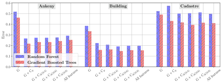
The misclassification errors for different sets of features are presented in Fig. 1, where we can see that color features bring a significant improvement. The best results are obtained with the features or with All features. A second important observation is that GBT consistently outperforms RF, in some cases by a large margin.
| Section | Ankeny | Building | Cadastre | |
|---|---|---|---|---|
| Geom. features | 67s | 23s | 46s | |
| Geom. + Color | 105s | 56s | 53s | |
| Random Forest (RF) | Train | 74s | 76s | 77s |
| Predict | 45s | 18s | 25s | |
| Boosted Trees (GBT) | Train | 5s | 5s | 5s |
| Predict | 56s | 23s | 41s |
Inter-dataset results
| Training Datasets | Testing Dataset | True Label | Predicted Label | Overall error | |||||
|---|---|---|---|---|---|---|---|---|---|
| Ground | High | Building | Road | Car | Human- | ||||
| vegetation | made object | ||||||||
| Building | ANKENY | Ground | 52% | 3.3% | 0.1% | 12% | 0.4% | 0.7% | 16.5% |
| Cadastre | High vegetation | 3.4% | 7.4% | 0.1% | 0.2% | 0.2% | 0.1% | 4.0% | |
| Human-made obj. | 0.4% | 0.3% | 0.1% | 0.1% | 0.2% | 0.1% | 1.1% | ||
| Ankeny | BUILDING | Building | 0.1% | 2.6% | 29% | 0.3% | 0.9% | 0.9% | 4.8% |
| Cadastre | Road | 2.2% | 0.3% | 0.02% | 33% | 0.3% | 0.3% | 3.1% | |
| Ground | 7.3% | 2.1% | 0.01% | 0.8% | 0.06% | 0.2% | 3.1% | ||
| Ankeny | CADASTRE | Ground | 32% | 2.1% | 6.6% | 4.6% | 0.9% | 4.7% | 18.9% |
| Building | High vegetation | 0.6% | 2.5% | 7.7% | 0.08% | 0.5% | 1.4% | 10.3% | |
| Road | 2.9% | 0.05% | 0.9% | 13% | 2.1% | 1.6% | 7.5% | ||
The results are shown in Fig. 2. First, there is an overall increase of classification error, in particular for the Cadastre dataset. To analyze the results in more detail we computed the confusion matrix for the top-3 classes that contribute to the misclassification error, as shown in Table 5. We now discuss the result of each dataset in detail.
Ankeny
The classifier performs very well for buildings and roads, as shown in Fig. 3(b). However it confuses large amounts of ground points as roads. This is not surprising since most of such mistakes occur in croplands, which are not present in any other dataset. Finally, although high vegetation appears in the top-3 misclassified classes in Table 5, this is mostly due to ambiguities in the ground truth: some bushes were manually labeled as ground, while the classifier predicts them as high vegetation.
Building
The classifier performs very well on this dataset. The highest error is due to predicting buildings as high vegetation or human-made objects. This dataset has the lowest GSD (or highest resolution), and facades of the buildings are well-reconstructed. This is not the case for the other two datasets with higher GSD, where few facade points are available. We hypothesize that the classifier is confused with the facades, finding the vegetation or human-made object to be the closest match.
Cadastre
The classifier predicts vast amounts of ground and vegetation points as buildings and human-made objects, leading to a very high error rate. This result is expected considering Table 3, as the Cadastre dataset contains hills and non-flat ground surfaces, which are not present in any of the other two datasets. Thus, the classifier confuses points in the regions of inclined ground with other classes that are closer in feature space to the training data (e.g. building roofs present a slope that resembles the properties of the points on a hill).
The analyses above highlight the importance of reliable and varied training data, in that it should resemble the unseen data on which the classifier will be applied, e.g different landscapes, seasons, shapes of buildings, etc.
4.5 Qualitative Results
R[1]¿\arraybackslashm#1
Ankeny dataset
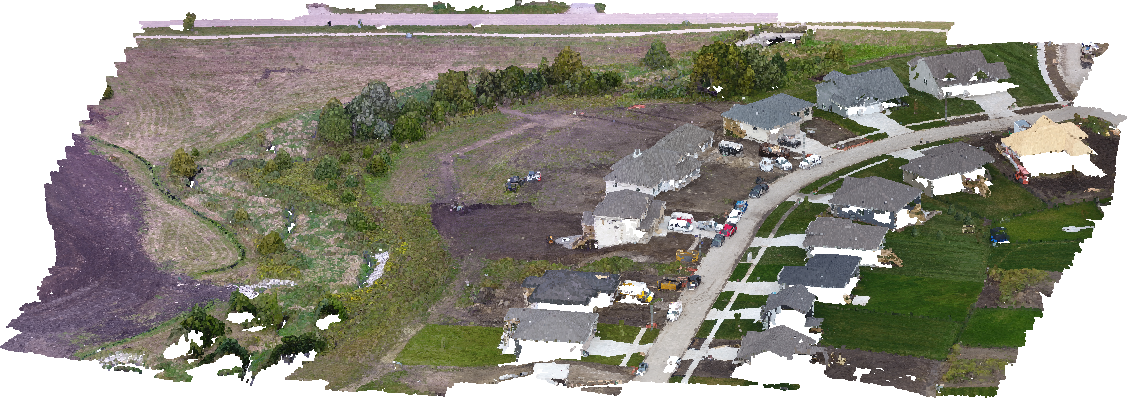
(a) Original data.
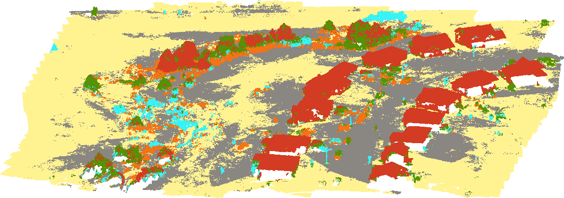
(b) Classification with geometry features only.
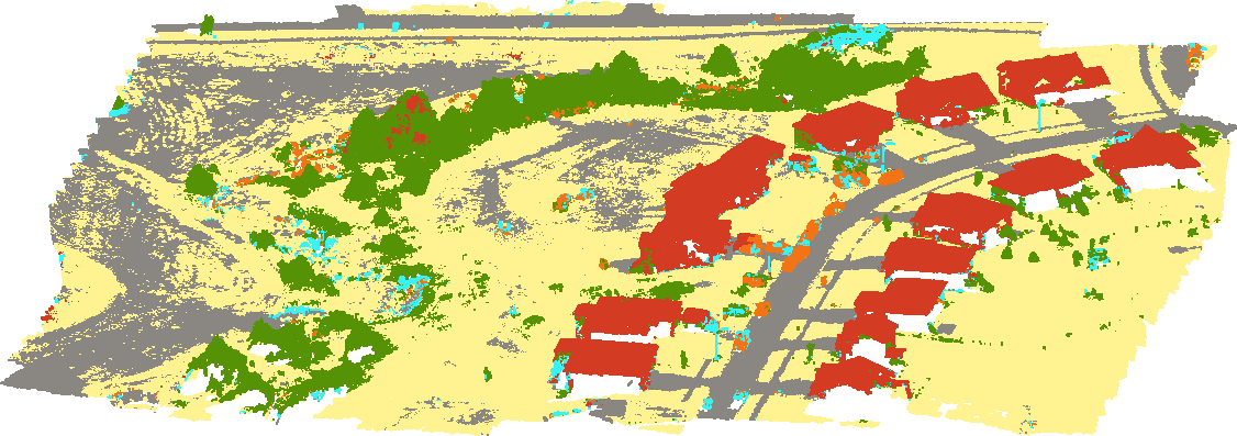
(c) Classification with geometry + color features.
| Ground | Road | Building | |||
| High veg. | Car | Human-made obj. |
Buildings dataset
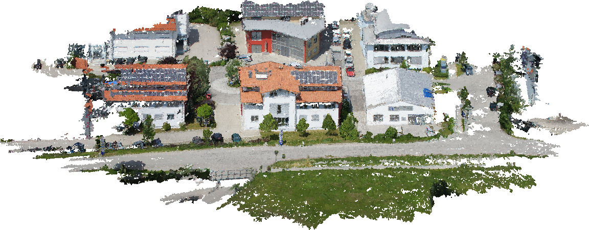
(a) Original data.
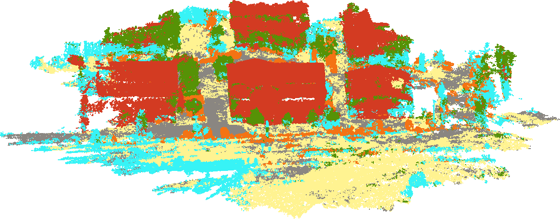
(b) Classification with geometry features only.
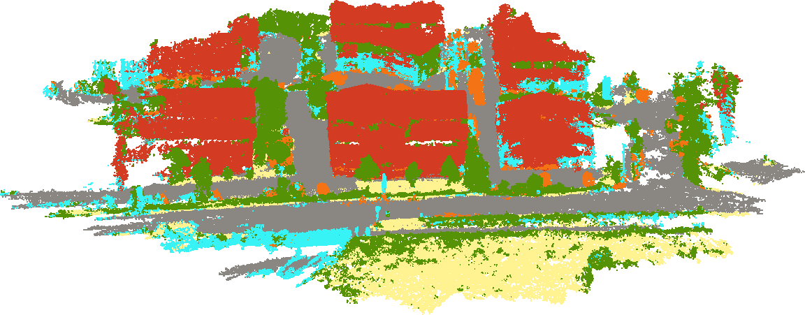
(c) Classification with geometry + color features.
| Ground | Road | Building | |||
| High veg. | Car | Human-made obj. |
Cadastre dataset
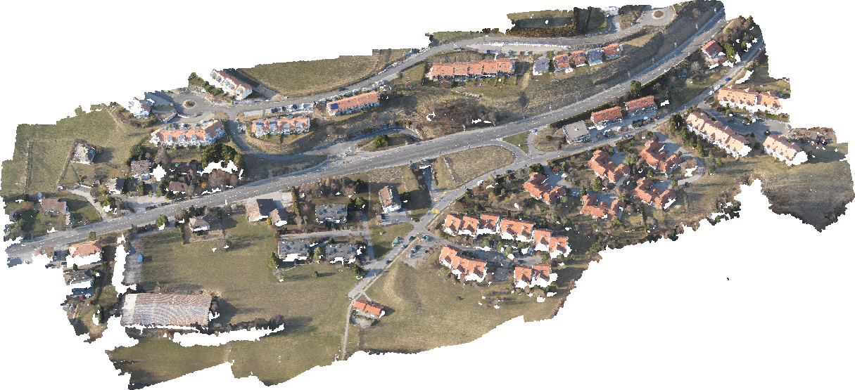
(a) Original data.
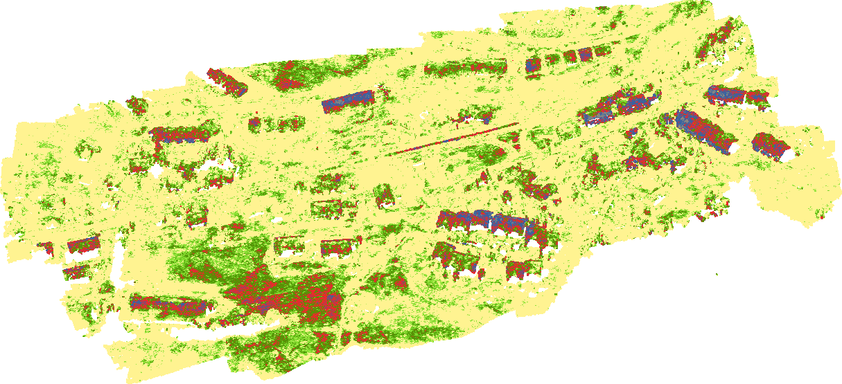
(b) Classification with geometry features only.
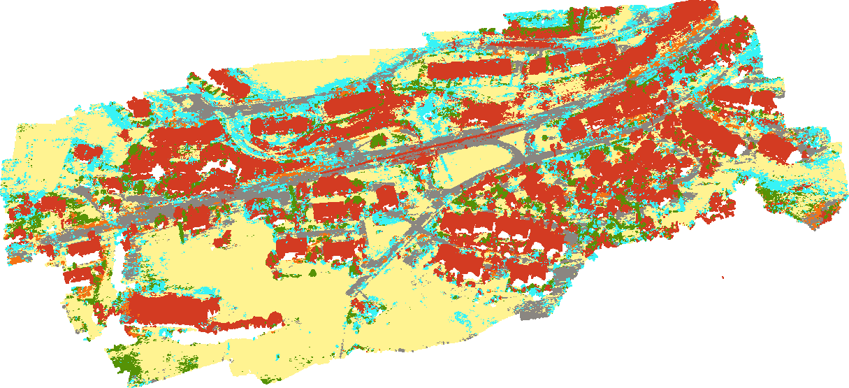
(c) Classification with geometry + color features.
| Ground | Road | Building | |||
| High veg. | Car | Human-made obj. |
Figures 3, 4 and 5 show 3D views of each dataset and the respective classified point clouds obtained when using geometric features only, as well as with our approach. Overall the results are very satisfying, especially when one considers the heterogeneity of the different datasets, as discussed earlier. These figures also help clarify the observations described in section 4.4. For example, grass and ground on slopes in Cadastre are sometimes misclassified as roof in Fig. 5(c).
4.6 Timings
Table 4 shows the break down of the timings obtained on a 6-core Intel i7 3.4 GHz computer. Our approach is very efficient, taking less than 3 minutes to classify every point in any of the presented photogrammetry datasets. This makes it ideal for the applications where the user needs to interact with the software to correct the training data or fix the classifier’s predictions.
| Testing dataset | Ankeny | Building | Cadastre | |
|---|---|---|---|---|
| Geom. features | 46% | 33% | 48% | |
| Geom. + Color | 24% | 16% | 41% |
5 Conclusion
In this paper we described an approach for a point-wise semantic labeling of aerial photogrammetry point clouds. The core contribution of our work is the use of color features, what improves significantly the overall classification results. Further we provide a concise comparison between two standard machine learning techniques that hopefully facilitates the decision making process of future research, showing that the Gradient Boosted Trees classifier outperforms the Random Forest classifier, in some cases by a large margin. Our method performs not only with high accuracies over the whole range of datasets used in the experiments but also with a high computational efficiency, making our approach suitable for interactive applications.
There are several directions that we would like to explore to increase accuracy and further decrease computational complexity. First we would like to explore the possibility to use auto-context information to train a second classifier that takes into account class labels of the neighboring points. Our preliminary experiments with this technique provided smoother results and higher accuracy. Another interesting topic to is to combine point cloud and image classification. Existing image classification algorithms are trained specifically to detect objects of such classes as cars and other human made objects. This method could increase the robustness of our classifier in particular on the classes that often confused: cars and human-made objects.
The classification method presented in this paper will soon be part of Pix4Dmapper Pro. Earlier we mentioned that access to properly labeled training data that represents aerial photogrammetry point clouds is limited. To overcome this issue we will implement an incremental training method, where users will be given the possibility to classify their data, visualize and correct errors manually. In a next step we will offer our users the possibility to include their datasets into our training data to improve the classifier quality. As the amount of training data increases we will be able not only to provide more accurate classifiers but to also train specialized ones. For example, we could provide a selection of classifiers for indoor and outdoor scenes, and for different seasons and scales.
References
- [Bezanson et al., 2014] Bezanson, J., Edelman, A., Karpinski, S. and Shah, V. B., 2014. Julia: A fresh approach to numerical computing. arXiv preprint arXiv:1411.1607.
- [Böhm et al., 2016] Böhm, J., Bredif, M., Gierlinger, T., Krämmer, M., Lindenberg, R., Liu, K., Michel, F. and Sirmacek, B., 2016. The IOMULUS urban showcase: automatic tree classification and identification in huge mobile mapping point points. ISPRS - International Archives of the Photogrammetry, Remote Sensing and Spatial Information Sciences XLI-B3, pp. 301–307.
- [Breiman, 2001] Breiman, L., 2001. Random Forests. Machine Learning 45(1), pp. 5–32.
- [Brenner, 2000] Brenner, C., 2000. Towards fully automatic generation of city models. In: In: IAPRS, pp. 85–92.
- [Brodu and Lague, 2012] Brodu, N. and Lague, D., 2012. 3D terrestrial LIDAR data classification of complex natural scenes using a multi-scale dimensionality criterion: Applications in geomorphology. ISPRS Journal of Photogrammetry and Remote Sensing 68, pp. 121–134.
- [Caruana and Niculescu-Mizil, 2006] Caruana, R. and Niculescu-Mizil, A., 2006. An empirical comparison of supervised learning algorithms. In: Proceedings of the 23rd international conference on Machine learning, ACM, pp. 161–168.
- [Dorninger and Nothegger, 2007] Dorninger, P. and Nothegger, C., 2007. 3d segmentation of unstructured point clouds for building modelling. International Archives of the Photogrammetry, Remote Sensing and Spatial Information Sciences 35(3/W49A), pp. 191–196.
- [eCognition, 2017] eCognition, 2017. Trimble, www.ecognition.com.
- [Friedman et al., 2001] Friedman, J., Hastie, T. and Tibshirani, R., 2001. The elements of statistical learning. Vol. 1, Springer series in statistics Springer, Berlin.
- [GlobalMapper, 2017] GlobalMapper, 2017. Blue marble geographics, www.bluemarblegeo.com.
- [Haala and Brenner, 1999] Haala, N. and Brenner, C., 1999. Extraction of buildings and trees in urban environments. ISPRS Journal of Photogrammetry and Remote Sensing 54, pp. 130–137.
- [Haala et al., 1998] Haala, N., Brenner, C. and Anders, K.-H., 1998. 3d urban GIS from laser altimeter and 2D map data. International Archives of Photogrammetry and Remote Sensing 32, pp. 339–346.
- [Hackel et al., 2016] Hackel, T., Wegner, J. D. and Schindler, K., 2016. Fast semantic segmentation of 3D point clouds with strongly varying density. ISPRS Annals of the Photogrammetry, Remote Sensing and Spatial Information Sciences, Prague, Czech Republic 3, pp. 177–184.
- [Hu and Yuan, 2016] Hu, X. and Yuan, Y., 2016. Deep-learning-based classification for dtm extraction from als point cloud. Remote Sensing 8(9), pp. 730.
- [Lafarge and Mallet, 2012] Lafarge, F. and Mallet, C., 2012. Creating Large-Scale City Models from 3D Point Clouds: A Robust Approach with Hybrid Representation. International Journal of Computer Vision 99(1), pp. 69–85.
- [Liu and Böhm, 2015] Liu, K. and Böhm, J., 2015. Classification of big point cloud data using cloud computing. The International Archives of Photogrammetry, Remote Sensing and Spatial Information Sciences 40(3), pp. 553.
- [Niemeyer et al., 2014] Niemeyer, J., Rottensteiner, F. and Soergel, U., 2014. Contextual classification of LIDAR data and building object detection in urban areas. ISPRS Journal of Photogrammetry and Remote Sensing 87, pp. 152–165.
- [Oesau et al., 2016] Oesau, S., Lafarge, F. and Alliez, P., 2016. Object classification via planar abstraction. ISPRS Annals of Photogrammetry, Remote Sensing and Spatial Information Sciences III-3, pp. 225–231.
- [Photoscan, 2017] Photoscan, 2017. Agisoft. www.agisoft.com.
- [Pix4Dmapper, 2017] Pix4Dmapper, 2017. Pix4D SA. www.pix4d.com.
- [Qi et al., 2016] Qi, C. R., Su, H., Mo, K. and Guibas, L. J., 2016. Pointnet: Deep learning on point sets for 3d classification and segmentation. arXiv preprint arXiv:1612.00593.
- [Rusu et al., 2009] Rusu, R. B., Blodow, N. and Beetz, M., 2009. Fast Point Feature Histograms (FPFH) for 3d registration. IEEE, pp. 3212–3217.
- [Rusu et al., 2007] Rusu, R. B., Blodow, N., Marton, Z., Soos, A. and Beetz, M., 2007. Towards 3D object maps for autonomous household robots. In: 2007 IEEE/RSJ International Conference on Intelligent Robots and Systems, IEEE, pp. 3191–3198.
- [Serna et al., 2014] Serna, A., Marcotegui, B., Goulette, F. and Deschaud, J.-E., 2014. Paris-rue-Madame database: a 3D mobile laser scanner dataset for benchmarking urban detection, segmentation and classification methods. In: 4th International Conference on Pattern Recognition, Applications and Methods ICPRAM 2014.
- [Shapovalov and Velizhev, 2011] Shapovalov, R. and Velizhev, A., 2011. Cutting-Plane Training of Non-associative Markov Network for 3d Point Cloud Segmentation. IEEE, pp. 1–8.
- [Shu et al., 2016] Shu, Z., Sun, K., Qiu, K. and Ding, K., 2016. Pairwise SVM for on-board urban road LIDAR classification. ISPRS - International Archives of the Photogrammetry, Remote Sensing and Spatial Information Sciences XLI-B1, pp. 109–113.
- [Sithole and Vosselman, 2003] Sithole, G. and Vosselman, G., 2003. Automatic structure detection in a point-cloud of an urban landscape. In: Remote Sensing and Data Fusion over Urban Areas, 2003. 2nd GRSS/ISPRS Joint Workshop on, IEEE, pp. 67–71.
- [Smith, 1978] Smith, A. R., 1978. Color gamut transform pairs. ACM SIGGRAPH Computer Graphics 12(3), pp. 12–19.
- [Tombari et al., 2010] Tombari, F., Salti, S. and Di Stefano, L., 2010. Unique signatures of histograms for local surface description. In: European conference on computer vision, Springer, pp. 356–369.
- [Unger et al., 2009] Unger, M., Pock, T., Grabner, M., Klaus, A. and Bischof, H., 2009. A Variational Approach to Semiautomatic Generation of Digital Terrain Models. In: D. Hutchison, T. Kanade, J. Kittler, J. M. Kleinberg, F. Mattern, J. C. Mitchell, M. Naor, O. Nierstrasz, C. Pandu Rangan, B. Steffen, M. Sudan, D. Terzopoulos, D. Tygar, M. Y. Vardi, G. Weikum, G. Bebis, R. Boyle, B. Parvin, D. Koracin, Y. Kuno, J. Wang, R. Pajarola, P. Lindstrom, A. Hinkenjann, M. L. Encarnação, C. T. Silva and D. Coming (eds), Advances in Visual Computing, Vol. 5876, Springer Berlin Heidelberg, Berlin, Heidelberg, pp. 1119–1130.
- [Vosselman et al., 2001] Vosselman, G., Dijkman, S. and others, 2001. 3D building model reconstruction from point clouds and ground plans. International archives of photogrammetry remote sensing and spatial information sciences 34(3/W4), pp. 37–44.
- [Wang and Schenk, 2000] Wang, Z. and Schenk, T., 2000. Building extraction and reconstruction from LIDAR data. International Archives of Photogrammetry and Remote Sensing 33(B3/2; PART 3), pp. 958–964.
- [Weinmann et al., 2013] Weinmann, M., Jutzi, B. and Mallet, C., 2013. Feature relevance assessment for the semantic interpretation of 3D point cloud data. ISPRS Annals of Photogrammetry, Remote Sensing and Spatial Information Sciences II-5/W2, pp. 313–318.
- [Weinmann et al., 2015a] Weinmann, M., Schmidt, A., Mallet, C., Hinz, S., Rottensteiner, F. and Jutzi, B., 2015a. Contextual classification of point cloud data by exploiting individual 3d neighborhoods. ISPRS Annals of Photogrammetry, Remote Sensing and Spatial Information Sciences II-3/W4, pp. 271–278.
- [Weinmann et al., 2015b] Weinmann, M., Urban, S., Hinz, S., Jutzi, B. and Mallet, C., 2015b. Distinctive 2D and 3D features for automated large-scale scene analysis in urban areas. Computers & Graphics 49, pp. 47–57.
- [Xiao and Furukawa, 2014] Xiao, J. and Furukawa, Y., 2014. Reconstructing the world’s museums. International Journal of Computer Vision 110(3), pp. 243–258.
- [Xu et al., 2016] Xu, Y., Tuttas, S., Heogner, L. and Stilla, U., 2016. Classification of photogrammetric point clouds of scaffolds for construction site monitoring using Subspace Clustering and PCA. ISPRS - International Archives of the Photogrammetry, Remote Sensing and Spatial Information Sciences XLI-B3, pp. 725–732.
- [Zhou et al., 2016] Zhou, M., Li, C. R., Ma, L. and Guan, H. C., 2016. Land cover classification from full-waveform LIDAR data based on Support Vector Machines. ISPRS - International Archives of the Photogrammetry, Remote Sensing and Spatial Information Sciences XLI-B3, pp. 447–452.