Trajectory-free approximation of phase space structures using the trajectory divergence rate

Abstract

This paper introduces the trajectory divergence rate, a scalar field which locally gives the instantaneous attraction or repulsion of adjacent trajectories. This scalar field may be used to find highly attracting or repelling invariant manifolds, such as slow manifolds, to rapidly approximating hyperbolic Lagrangian coherent structures, or to provide the local stability of invariant manifolds. This work presents the derivation of the trajectory divergence rate and the related trajectory divergence ratio for 2-dimensional systems, investigates their properties, shows their application to several example systems, and presents their extension to higher dimensions.

1 Introduction

To better understand the properties of mathematical models and experimental measurements, it is often convenient to look at the geometric structure of the flow of a resulting vector field. There often exist lower-dimensional manifolds which dominate the attraction and repulsion, swirling, or shearing of trajectories advecting under the flow. Methods to find such structures have been applied to better understand topics including plant pathogen spread schmale2015highways, animal locomotion nave2018global; peng2008theupstream, seabird foraging patterns kai2009top, geophysical flows lekien2005pollution; wiggins2005dynamical, chemical reactions zhong2017tube, comet distributions dellnitz2005transport, and structural mechanics wiggins2001impenetrable.

In autonomous systems, the simplest geometric structure of interest is the fixed point, which is a 0-dimensional invariant manifold in the flow. Stable, unstable, and center manifolds of a fixed point may be calculated through a number of classical methods, including “growing” the stable or unstable manifolds by integrating the eigendirections of fixed points backward or forward in time koon2008dynamical. However, in the context of weak stable submanifolds, these methods begin to break down nave2018global. Some weak submanifolds are part of a class of geometric structures known as slow manifolds which exhibit a separation of time scales kuehn2016multiple, attracting or repelling other trajectories in phase space. This difference in time scales between motion along a slow manifold and the motion normal to it allows them to be classified as normally hyperbolic invariant manifolds (NHIMs) wiggins2013normally.

Geometric structure may also be present in the absence of fixed points or slow manifolds. Recent developments in dynamical systems have led to several useful generalizations of some key geometric features. Distinguished hyperbolic trajectories generalize stable and unstable manifolds to aperiodic flows, and are identified using the “$M$-function” madrid2009distinguished. Hyperbolic coherent structures represent dynamically evolving transport barriers in flows shadden2011lagrangian; shadden2005definition. Although the methods of coherent structures are typically situated within the context of fluid dynamics, such structures have applications to the flow of general vector fields aldridge2006direct; gawlik2009lagrangian; nave2018global; tanaka2010mathematical. Detecting and analyzing the underlying structures of flows gives a better understanding of how the system evolves, whether that flow represents the motion of a fluid or some other general dynamical system.

Methods to identify coherent structures may be based on integrated trajectory information or may be calculated from the instantaneous vector field for the entire volume. Most state of the art methods are trajectory-based, using finite-time integration of trajectories to calculate coherent structures balasuriya2018generalized; shadden2011lagrangian. There is a wide variety of trajectory-based methods to identify coherent structures or coherent sets, including transfer operator methods dellnitz2001algorithms; froyland2015rough, topological methods allshouse2012detecting; budivsic2015finite, and stretching-based methods such as the finite-time Lyapunov exponent (FTLE) shadden2005definition; see Hadjighasem et al. hadjighasem2017critical for a review. Lagrangian descriptors, similarly, calculate properties of the flow along trajectories and can be used to detect “distinguished trajectories” lopesino2017theoretical; madrid2009distinguished. However, trajectory-based methods involve significant computational resources, requiring trajectory integration over an ensemble of initial conditions ameli2014development; brunton2010fast.

There is much to be gained by looking at the instantaneous information of vector fields. Although the trajectory-dependent coherent structures are more robust to the flow, the short time behavior of these structures may be of interest haller2010localized. Vector field schemes are also much more computationally efficient, and their changes can be tracked in time for nonautonomous flows. Historically, most vector field-based methods have focused on elliptic, or vortex-like, coherent structures chakraborty2005relationships. More recent work has developed the notion of objective Eulerian coherent structures for 2-dimensional flows serra_objective_2016, which include hyperbolic and parabolic structures in addition to objectively defined elliptic coherent structures. However, while objectivity is necessary for detecting, for instance, vortex-like coherent structures in a fluid, objectivity may be a disadvantage in other examples of dynamical systems haller_variational_2011; lopesino2017theoretical.

1.1 Main result

This paper introduces the trajectory divergence rate for 2-dimensional vector fields, given by,

$$\dot{\rho}=\mathbf{n}^{\dagger}\mathbf{S}\mathbf{n},$$

where $\mathbf{n}=\mathbf{R}\mathbf{v}/\left|\mathbf{v}\right|$ is the unit normal vector field, with $R=\left(\begin{smallmatrix}0&-1\\ 1&0\end{smallmatrix}\right)$ giving a $90^{\circ}$ rotation, and $\mathbf{S}=\tfrac{1}{2}\left(\nabla\mathbf{v}+(\nabla\mathbf{v})^{\dagger}\right)$ is the rate-of-strain tensor, representing the symmetric component of the Jacobian of the system. In this work, the dagger, $(\cdot)^{\dagger}$, indicates the matrix transpose to avoid confusion with time-integrated methods. The trajectory divergence rate is an inherent property of $C^{1}$ vector fields, measuring the extent to which the trajectory passing through each point instantaneously repels or attracts nearby trajectories. This paper will show that this quantity may be used as a diagnostic tool to approximate slow manifolds and hyperbolic coherent structures by showing regions of strong instantaneous repulsion or attraction.

Instantaneous attraction and repulsion has been considered previously, through other metrics such as the normal infinitesimal Lyapunov exponent (NILE) haller2010localized and the strain acceleration tensor haller2001lagrangian. These methods have primarily been applied to partition the space or look into regions of local stability or instability, particularly within applications of turbulence. The trajectory divergence rate introduced herein is intended to serve as a “rough and ready” method for approximating hyperbolic, or stretching-based, geometric structures in the flows of general nonlinear dynamical systems. Much like local curvature desroches2011canards, this quantity may be thought of as an inherent property of continuously differentiable vector fields, showing the instantaneous local divergence or convergence of nearby trajectories. Under certain conditions, the regions of highest local divergence or convergence serve to approximate finite-time coherent structures.

The idea of stability is asymptotic in nature; a stable invariant manifold is one for which nearby trajectories stay close for $t\to\infty$. Although transport barriers and invariant manifolds in flows are calculated based on the long-term dynamics of the system, and therefore the long-term repulsion of the manifold in question, the instantaneous repulsion of invariant manifolds provides additional insights into the character of an invariant manifold, as regions of a globally attracting invariant manifold may be instantaneously repelling haller2001lagrangian; tallapragada2017globally. The trajectory divergence rate is easily computable, requiring only the vector field and its gradient, and can serve as a useful diagnostic in the search for influential geometric structures in flows.

Section 2 gives the mathematical preliminaries and notation to provide the mathematical context for the divergence rate. Section 3 shows the derivation of the trajectory divergence rate and discusses its properties. Section 4 shows several applications of the divergence rate over a different situations in which it may prove useful. Section LABEL:s:HigherDimension extends the trajectory divergence rate from 2-dimensional to higher dimensional systems and provides a 3-dimensional example. Finally, Section LABEL:s:Summary provides some discussion about the work of this paper to conclude the work.

2 Background and notation

To begin, consider a general 2-dimensional, autonomous ordinary differential equation

$$\mathbf{\dot{x}}=\mathbf{v}(\mathbf{x}),\quad\mathbf{x}\in U\subseteq\mathbb{R}^{2},\,t\in\mathbb{R},$$ (1)

with its time-$T$ mapping all initial conditions forward to their positions after a duration $T$,

$$\begin{split}&\mathbf{F}_{T}:U\rightarrow U,\quad T\in\mathbb{R},\\ &\mathbf{x}_{0}\mapsto\mathbf{x}_{T}=\mathbf{x}(T;\mathbf{x}_{0}).\end{split}$$ (2)

For any $\mathbf{x}\in U$ with $\mathbf{v}(\mathbf{x})\neq\mathbf{0}$ (that is, excluding equilibrium points), one can define the following unit vector fields parallel and normal to the governing vector field $\mathbf{v}(\mathbf{x})$, respectively,

$$\begin{split}&\mathbf{e}(\mathbf{x})=\frac{\mathbf{v}(\mathbf{x})}{|\mathbf{v}(\mathbf{x})|},\\ &\mathbf{n}(\mathbf{x})=\mathbf{R}\mathbf{e}(\mathbf{x}),\quad\mathbf{R}=\left(\begin{array}[]{cc}0&-1\\ 1&~{}0\end{array}\right).\end{split}$$ (3)

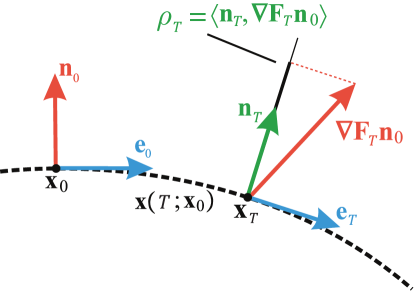
The gradient of the time-$T$ flow map $\nabla\mathbf{F}_{T}$ defines a mapping from vectors based at $\mathbf{x}_{0}$, such as $\mathbf{e}(\mathbf{x}_{0})$ and $\mathbf{n}(\mathbf{x}_{0})$, to vectors based at $\mathbf{x}_{T}$, showing how those vectors deform with the flow. The tangent vector, in general, maps to the new tangent direction, but the normal vector does not map to the normal direction at time $T$ due to the shear of the flow.

2.1 Trajectory-normal repulsion rate

For any trajectory passing through a point $\mathbf{x}_{0}\in U$ with $\mathbf{v}(\mathbf{x}_{0})\neq\mathbf{0}$, the trajectory-normal repulsion rate $\rho_{T}(\mathbf{x}_{0})$ haller_variational_2011 over the time interval $[0,T]$ may be defined locally as the projection of $\nabla\mathbf{F}_{T}(\mathbf{x}_{0})\mathbf{n}_{0}$ onto the new normal vector $\mathbf{n}_{T}$,

$$\rho_{T}(\mathbf{x}_{0})=\langle\mathbf{n}_{T},\nabla\mathbf{F}_{T}(\mathbf{x}_{0})\mathbf{n}_{0}\rangle,$$ (4)

where $\mathbf{n}_{T}=\mathbf{n}(\mathbf{x}_{T})=\mathbf{n}(\mathbf{F}_{T}(\mathbf{x}_{0}))$ and $\langle\cdot,\cdot\rangle$ is the usual inner product in $\mathbb{R}^{2}$. As illustrated in Figure 1, $\rho_{T}(\mathbf{x}_{0})$ is a measure of the growth of infinitesimal perturbations normal to the invariant manifold containing $\mathbf{x}_{0}$ over the time interval $[0,T]$. If the projection $\rho_{T}(\mathbf{x}_{0})>1$, then infinitesimal perturbations normal to the trajectory through $\mathbf{x}_{0}$ grow over the time interval $[0,T]$. Note that, although overall growth over the duration $T$ may be repelling (attracting), it is possible for the invariant manifold to be instantaneously attracting (repelling) tallapragada2017globally.

Figure 1: Geometry of the trajectory-normal repulsion rate, reproduced from nave2018global.

This scalar field $\rho_{T}(\mathbf{x}_{0})$ can be used to extract the most influential invariant manifolds in the flow, in the sense that it reveals those manifolds that normally repel (or attract) other manifolds at the largest rate. Using this trajectory-normal repulsion rate, one can calculate, for example, slow-manifolds, such as those found in the examples below.

2.2 Trajectory-normal repulsion ratio

A related quantity is the trajectory-normal repulsion ratio haller_variational_2011, which is the ratio of normal repulsion to the tangential stretching along an invariant manifold passing through the point $\textbf{x}_{0}$ over the time interval $[0,T]$,

$$\nu_{T}(\mathbf{x}_{0})=\frac{\rho_{T}(\mathbf{x}_{0})}{\left|\nabla\mathbf{F}_{T}(\mathbf{x}_{0})\mathbf{e}_{0}\right|}.$$ (5)

Where the trajectory-normal repulsion ratio $\nu_{T}(\mathbf{x}_{0})>1$, the normal stretching dominates the tangential stretching of the curve.

Both the trajectory-normal repulsion rate and trajectory-normal repulsion ratio can be written in terms of the right Cauchy-Green tensor $\mathbf{C}_{T}(\mathbf{x}_{0})$, well-known from continuum mechanics truesdell2004non, as well as its use in FTLE and LCS calculations haller_variational_2011,

$$\rho_{T}(\mathbf{x}_{0}) =\sqrt{\frac{\left|\mathbf{v}(\mathbf{x}_{0})\right|^{2}{\rm det}\mathbf{C}_{T}(\mathbf{x}_{0})}{\langle\mathbf{v}(\mathbf{x}_{0}),\mathbf{C}_{T}(\mathbf{x}_{0})\mathbf{v}(\mathbf{x}_{0})\rangle}}$$ (6)

$$\nu_{T}(\mathbf{x}_{0}) =\frac{\left|\mathbf{v}(\mathbf{x}_{0})\right|^{2}\sqrt{{\rm det}\mathbf{C}_{T}(\mathbf{x}_{0})}}{\langle\mathbf{v}(\mathbf{x}_{0}),\mathbf{C}_{T}(\mathbf{x}_{0})\mathbf{v}(\mathbf{x}_{0})\rangle}$$

As a matter of notation, in this work $(\cdot)_{T}$ will indicate a value calculated over the interval $[0,T]$. Note that $T$ may be positive or negative. Because of their dependence on the normal vector in the derivation of these expressions, these scalar fields both remain defined only for 2-dimensional systems.

When both $\rho_{T}(\mathbf{x})>1$ and $\nu_{T}(\mathbf{x})>1$ for all $\mathbf{x}\in\gamma$, where $\gamma$ is an invariant manifold, and $\gamma$ is a ridge of the $\rho_{T}$-field, $\gamma$ is a constrained Lagrangian coherent structure haller_variational_2011, in the sense that the variational search for attracting or repelling curves is constrained to the space of invariant manifolds.

3 The trajectory divergence rate

The trajectory-normal repulsion rate $\rho_{T}$ may be useful in finding attracting (or repelling) structures in a 2-dimensional flow haller_variational_2011, but calculation of the time-$T$ flow map over the domain of interest is computationally expensive. Therefore, this work seeks an instantaneous measure that gives the leading order behavior of this scalar field.

Figure 2: This schematic shows the relationship between the divergence rate and the time-$T$ repulsion rate $\rho_{T}$. The divergence rate is the instantaneous rate of change of the repulsion rate, which is therefore signified as $\dot{\rho}$.

For scalar and tensor fields, the dependence on $\mathbf{x}_{0}$ will be notationally dropped for clarity, as it will be understood. For small time $T$, the right Cauchy-Green tensor, $\mathbf{C}_{T}$, may be expanded in terms of integration time $T$,

$$\mathbf{C}_{T}=\mathbf{C}_{0}+\left.\frac{d\mathbf{C}_{T}}{dT}\right|_{T=0}T+\frac{1}{2}\left.\frac{d^{2}\mathbf{C}_{T}}{dT^{2}}\right|_{T=0}T^{2}+\cdots$$ (7)

Because all derivatives are evaluated at $T=0$, $\left.\tfrac{d}{dt}\right|_{t=0}=\left.\tfrac{d}{dT}\right|_{t=0}$. The derivatives of the right Cauchy-Green tensor are given by the Rivlin-Ericksen tensors truesdell2004non,

$$\frac{d^{k}\mathbf{C}_{T}}{dt^{k}} =\nabla\frac{d\mathbf{x}}{dt}+\left(\nabla\frac{d\mathbf{x}}{dt}\right)^{\dagger}, k=1,$$ (8)

$$\frac{d^{k}\mathbf{C}_{T}}{dt^{k}} =\nabla\frac{d^{k}\mathbf{x}}{dt^{k}}+\left(\nabla\frac{d^{k}\mathbf{x}}{dt^{k}}\right)^{\dagger}$$

$$+\sum_{i=1}^{k-1}\left(\!\begin{array}[]{c}k\\ i\end{array}\!\right)\left(\nabla\frac{d^{i}\mathbf{x}}{dt^{i}}\right)^{\dagger}\nabla\frac{d^{k-i}\mathbf{x}}{dt^{k-i}}, k\geq 2.$$

For small $T\ll 1$, the leading order behavior is given by the first Rivlin-Ericksen tensor $(\nabla\mathbf{v}+(\nabla\mathbf{v})^{\dagger})$. Neglecting higher order dependence on $T$, the expansion of the Cauchy-Green tensor (7) simplifies to,

$$\mathbf{C}_{T}=\mathbf{I}+2\mathbf{S}T+\mathcal{O}(T^{2}),$$ (9)

where $\mathbf{S}$ represents the symmetric rate-of-strain tensor, defined as,

$$\mathbf{S}=\tfrac{1}{2}\left(\nabla\mathbf{v}+\nabla\mathbf{v}^{\dagger}\right).$$ (10)

Note that in $\mathbb{R}^{2}$, we will denote the eigenvalues of $\mathbf{S}$ as $s_{1},s_{2}$, with $s_{1}\leq s_{2}$.

The expansion of the Cauchy-Green tensor in (7) makes it possible to perform a Taylor expansion of the trajectory-normal repulsion rate, $\rho_{T}$ from (4) and Fig. 1 for a small integration time $T\ll 1$. For a 2-dimensional system, the following identity allows the expansion of the determinant within the trajectory-normal repulsion rate,

$${\rm det}(\mathbf{A}+\mathbf{B})={\rm det}\mathbf{A}+{\rm det}\mathbf{B}+{\rm det}\mathbf{A}\cdot{\rm tr}(\mathbf{A}^{-1}\mathbf{B}),$$ (11)

Neglecting the higher order dependence on $T$ in (9) admits the substitution $\mathbf{C}_{T}=\mathbf{I}+2T\mathbf{S}$. Therefore, $\det\mathbf{C}_{T}$, can be expressed as,

$$\det\mathbf{C}_{T} =\det(\mathbf{I}+2T\mathbf{S})$$ (12)

$$=\det(\mathbf{I})+\det(2T\mathbf{S})+\det(\mathbf{I})\text{tr}(2T\mathbf{I}^{-1}\mathbf{S})$$

$$=1+4T^{2}\det(\mathbf{S})+2T\text{tr}(\mathbf{S})$$

$$=1+2T\text{tr}(\mathbf{S})+\mathcal{O}(T^{2}).$$

To finish the expansion of (6), the same substitution $\mathbf{C}_{T}=\mathbf{I}+2T\mathbf{S}$ gives the following result.

$$\frac{\left|\mathbf{v}\right|^{2}}{\mathbf{v}^{\dagger}\mathbf{C}_{T}\mathbf{v}} =\frac{\left|\mathbf{v}\right|^{2}}{\left|\mathbf{v}\right|^{2}+2T\mathbf{v}^{\dagger}\mathbf{S}\mathbf{v}+\mathcal{O}(T^{2})}$$ (13)

$$=\frac{1}{1+\frac{1}{\left|\mathbf{v}\right|^{2}}2T\mathbf{v}^{\dagger}\mathbf{S}\mathbf{v}+\mathcal{O}(T^{2})}$$

$$=1-2T\frac{\mathbf{v}^{\dagger}\mathbf{S}\mathbf{v}}{\left|\mathbf{v}\right|^{2}}+\mathcal{O}(T^{2})$$

Combining these two substitutions gives the following relation for the trajectory-normal repulsion ratio.

$$\rho_{T} =\sqrt{\frac{|\mathbf{v}|^{2}\det\mathbf{C}_{T}}{\mathbf{v}^{\dagger}\mathbf{C}_{T}\mathbf{v}}}$$ (14)

$$=\sqrt{\left(1+2T\text{tr}\left(\mathbf{S}\right)+\mathcal{O}(T^{2})\right)\left(1-2T\frac{\mathbf{v}^{\dagger}\mathbf{S}\mathbf{v}}{\left|\mathbf{v}\right|^{2}}+\mathcal{O}(T^{2})\right)}$$

$$=1+\left(\text{tr}(\mathbf{S})-\frac{\mathbf{v}^{\dagger}\mathbf{S}\mathbf{v}}{\left|\mathbf{v}\right|^{2}}\right)T+\mathcal{O}(T^{2})$$

Neglecting higher order terms for small $T$,

$$\rho_{T}=1+\left(\text{tr}(\mathbf{S})-\frac{\mathbf{v}^{\dagger}\mathbf{S}\mathbf{v}}{\left|\mathbf{v}\right|^{2}}\right)T$$ (15)

Therefore, the leading order behavior of $\rho_{T}$ for small $T$ is given entirely by the quantity $\dot{\rho}=\left.\frac{d\rho_{T}}{dT}\right|_{T=0}$,

$$\dot{\rho}=\text{tr}(\mathbf{S})-\frac{\mathbf{v}^{\dagger}\mathbf{S}\mathbf{v}}{\left|\mathbf{v}\right|^{2}}$$ (16)

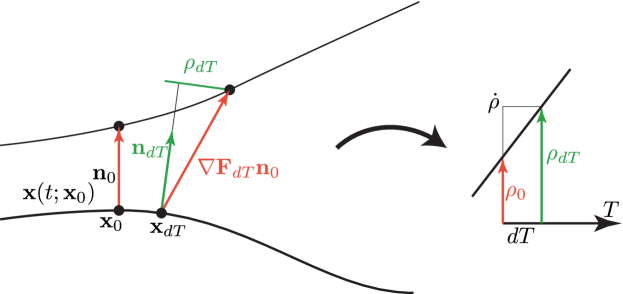
which is the trajectory divergence rate. Fig. 2 shows a schematic of the geometric interpretation of this derivation.

This quantity is independent of the choice of the time parameter $T$, and, furthermore, does not require integration to be calculated. It is dependent solely on the given vector field $\mathbf{v}(\mathbf{x})$ and its gradient through the rate-of-strain tensor $\mathbf{S}$. As shown in Appendix LABEL:ap:_normal_derivation, for 2-dimensional systems, this expression reduces to simply

$$\dot{\rho}=\mathbf{n}^{\dagger}\mathbf{S}\mathbf{n}$$ (17)

The instantaneous rate of normal repulsion is given by a quadratic form on the rate-of-strain tensor by the unit normal vector. The trajectory divergence rate can also be derived via the following expression for the rate of change of length of an infinitesimal vector $\ell$,

$$\frac{1}{2}\frac{d}{dt}\left|\ell\right|^{2}=\ell^{\dagger}\mathbf{S}\ell.$$ (18)

3.1 Trajectory divergence ratio

Following the same procedure as the expansion of the repulsion rate, the trajectory-normal repulsion ratio may be expanded by,

$$\nu_{T}=\frac{\left|\mathbf{v}\right|^{2}\sqrt{{\rm det}\mathbf{C}_{T}}}{\langle\mathbf{v},\mathbf{C}_{T}\mathbf{v}\rangle},$$ (19)

for small $T$ to find its instantaneous rate of growth. From (12),

$$\sqrt{\det\mathbf{C}_{T}}=1+T\text{tr}(\mathbf{S})+\mathcal{O}(T^{2}),$$ (20)

and using (13),

$$\nu_{T} =\left(1+T\text{tr}(\mathbf{S})+\mathcal{O}(T^{2})\right)\left(1-2T\frac{\mathbf{v}^{\dagger}\mathbf{S}\mathbf{v}}{\left|\mathbf{v}\right|^{2}}+\mathcal{O}(T^{2})\right)$$ (21)

$$=1+T\left(\text{tr}(\mathbf{S})-2\frac{\mathbf{v}^{\dagger}\mathbf{S}\mathbf{v}}{\left|\mathbf{v}\right|^{2}}\right)+\mathcal{O}(T^{2})$$

And the rate of $\nu_{T}$ is given as

$$\dot{\nu}=\frac{\mathbf{v}^{\dagger}\left(\text{tr}(\mathbf{S})\mathbf{I}-2\mathbf{S}\right)\mathbf{v}}{\left|\mathbf{v}\right|^{2}}$$ (22)

Similar to the trajectory divergence rate $\dot{\rho}$, the trajectory divergence ratio is dependent only on the rate-of-strain tensor and therefore does not require the calculation of trajectories. These scalar fields give a measurement of the instantaneous stretching of normal vectors throughout phase space and can be used to find the most attracting and repelling structures with much less computational cost.

3.2 Physical interpretation of the trajectory divergence rate

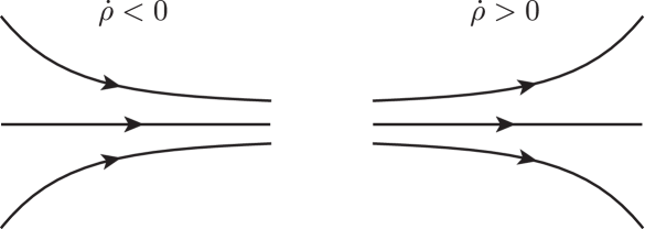
The trajectory divergence rate provides a scalar measurement of how much a trajectory is attracting or repelling nearby trajectories, representing the time-normalized slope of the normal distance between nearby trajectories, as visualized in Figure 2. Therefore, as shown in Figure 4, a positive divergence rate indicates diverging trajectories, a negative divergence rate indicates converging trajectories, and a zero divergence rate shows the regions of the flow where trajectories are parallel. To visualize this, consider the simple linear saddle flow.

Figure 3: The phase portrait (top) and trajectory divergence rate field (bottom) for Example 1.

Example 1

– Linear saddle flow.
The saddle-point flow represents the simplest case of stable and unstable manifolds. The system is given by

$$\dot{x} =x,$$ (23)

$$\dot{y} =-y.$$

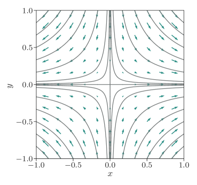
As is visible in Figure 3, the linear saddle flow repels trajectories from the $y$-axis and attracts them to the $x$-axis in forward time.

The unit normal vector and rate-of-strain tensor are given by

$$\mathbf{n}=\frac{1}{\sqrt{x^{2}+y^{2}}}\left[\begin{array}[]{c}y\\ x\end{array}\right],\quad\mathbf{S}=\left[\begin{array}[]{cc}1&0\\ 0&-1\end{array}\right].$$ (24)

From these, the trajectory divergence rate is computed to be,

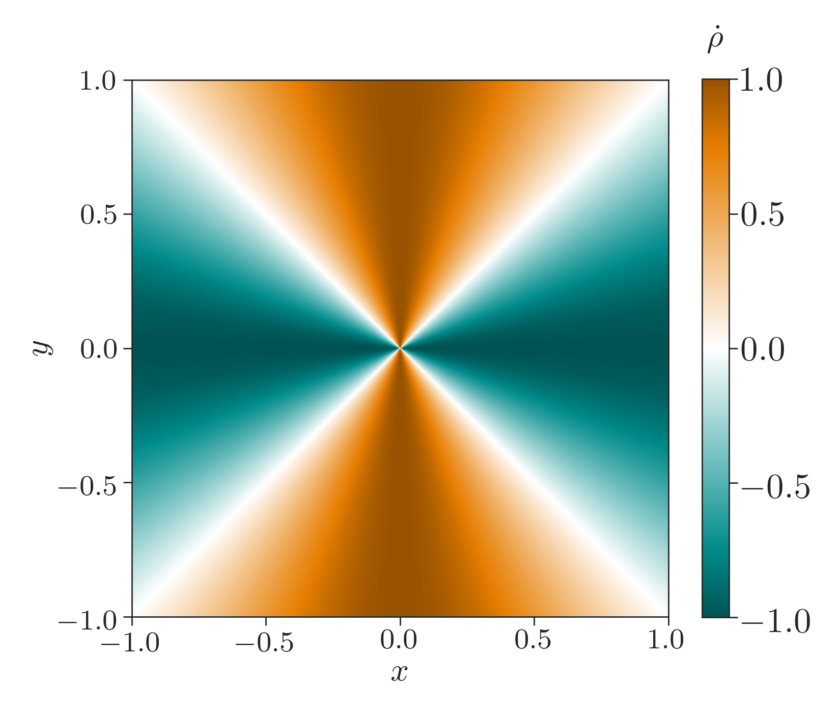
$$\dot{\rho}=\frac{y^{2}-x^{2}}{x^{2}+y^{2}}.$$ (25)

Figure 3 shows trajectories in phase space and the trajectory divergence rate of the linear saddle. From (25) and the trajectory divergence rate in the figure, trajectories are converging when $x^{2}>y^{2}$ and diverging when $y^{2}>x^{2}$. Trajectories are parallel where $y=\pm x$, as shown in white. The ridges and troughs of the trajectory divergence rate field give the most repelling and attracting curves in the field: the vertical and horizontal axes, respectively. Interestingly, the forward and backward finite-time Lyapunov exponents are both uniform for the linear saddle flow, indicating no structure haller_variational_2011.

Figure 4: Schematic of the physical interpretation of the trajectory divergence rate $\dot{\rho}$. Negative values indicate converging trajectories while positive values indicate diverging trajectories.

3.3 Remarks on the trajectory divergence rate

3.3.1 (Lack of) objectivity of the trajectory divergence rate

The trajectory divergence rate (17) is not an objective quantity, as a scalar quantity such as $\dot{\rho}$ would be objective only if it remained unchanged under any translation and rotation of reference frame truesdell2004non; serra_objective_2016. In other words, objective scalar values remain invariant under transformations belonging to the Special Euclidean group $SE(n)$. Because the trajectory divergence rate depends on the tangent vectors, which are not objective, the quantity itself is not objective. However, as shown in the context of Lagrangian descriptors, objectivity is not always a desirable trait lopesino2017theoretical. For the example of a rotating saddle flow, the finite-time Lyapunov exponent, which is an objective quantity, gives no structure at all. However, in that example, Lagrangian descriptors, which are not objective, are able to show the rotating saddle at every snapshot in time. Under situations where objectivity is necessary, the trajectory divergence rate may not be the appropriate tool to use. However, objectivity is not always a desirable property, and makes no sense in general abstract phase spaces.

3.3.2 Relationship to Objective Eulerian Coherent Structures

In their paper introducing objective Eulerian coherent structures serra_objective_2016, Serra and Haller introduce two objective quantities to calculate these structures: the stretching rate $\dot{p}$ and shear rate $\dot{q}$. These equations depend on the tangent vectors $x^{\prime}$ of a general curve $\gamma$ parametrized by its arc length $s$.

$$\dot{p}=\frac{\langle x^{\prime}(s),\mathbf{S}x^{\prime}(s)\rangle}{\langle x^{\prime}(s),x^{\prime}(s)\rangle}$$ (26)

$$\dot{q}=\frac{\langle x^{\prime}(s),\left(\mathbf{S}\mathbf{R}-\mathbf{R}\mathbf{S}\right)x^{\prime}(s)\rangle}{\langle x^{\prime}(s),x^{\prime}(s)\rangle}$$ (27)

These scalar functions are objective because they depend generally on $\mathbf{S}$, which is an objective tensor, and tangent vectors to a curve $\gamma$, which is not dependent on the vector field. If these curves are restricted to trajectories following the vector field rather than general curves, then their tangent vectors become the vector field $x^{\prime}=\mathbf{v}$, and $\dot{p}$ and $\dot{q}$ become quadratic forms on vectors $\mathbf{v}$ like the trajectory divergence rate and trajectory divergence ratio. However, they lose the objectivity that is central to the previous work. As discussed above, there are situations where objectivity is less important, so trajectory-based variations of the stretch rate $\dot{p}_{v}$ and shear rate $\dot{q}_{v}$ which depend on the vector field may prove useful. Considering the unit tangent vector $\mathbf{e}=\mathbf{v}/\left|\mathbf{v}\right|$, these are given by,

$$\dot{p}_{v} =\langle\mathbf{e},\mathbf{S}\mathbf{e}\rangle,$$ (28)

$$\dot{q}_{v} =\langle\mathbf{e},\left(\mathbf{S}\mathbf{R}-\mathbf{R}\mathbf{S}\right)\mathbf{e}\rangle.$$

Together with the trajectory divergence rate introduced above, these three quadratic forms measure the instantaneous rates of tangential stretching, normal stretching, and shear of the vector field. The trajectory stretch rate $\dot{p}_{v}$ and trajectory shear rate $\dot{q}_{v}$ are worth further exploration in future studies.

3.3.3 Normal hyperbolicity of trajectories

On the other hand, removing the restriction of the trajectory divergence rate to trajectories of the vector field to instead calculate the normal repulsion of a general surface, the trajectory divergence rate becomes an objective scalar value just like the stretching and shear rates above. In fact,the expression for the trajectory divergence rate in Eq. (17) is similar to an existing quantity has been applied to normal vectors of candidate Lagrangian coherent structure as a test of hyperbolicity, using gradients of the finite-time Lyapunov exponent field to determine the tangent and normal directions green2010using. The trajectory divergence rate, in contrast, uses the vector normal to trajectories of the underlying dynamical system. From this observation, it is clear that the trajectory divergence rate gives the normal hyperbolicity field of the vector field. Because of this, the trajectory divergence rate may be a useful metric for finding normally hyperbolic structures in a flow. This idea is explored further in Sec. 4.1.

4 Applications of the trajectory divergence rate

As a measure of normal attraction and repulsion of trajectories of a system, the trajectory divergence rate can be applied to a variety of special cases to identify influential structures in dynamical systems. It may serve as a good approximation for hyperbolic Lagrangian coherent structures or as a method to identify slow manifolds. Additionally, it may be relevant to calculate the normal hyperbolicity of a particular trajectory for applications in control.

4.1 Approximation of slow manifolds and normally hyperbolic invariant manifolds

Given the interpretation of the trajectory divergence rate as a measure of normal hyperbolicity, it becomes a natural tool to identify normally hyperbolic invariant manifolds (NHIMs). One of the key examples of NHIMs is in the study of slow manifolds of multiple time scale systems kuehn2016multiple. In such systems there is a lower-dimensional manifold on which most of the dynamics occur, referred to as the slow manifold. This is typically conceptualized as an attracting manifold, but may be repelling in some cases. Outside of the slow manifold, the motion moves more quickly onto (or away from) the slow manifold.

Figure 5: (Left) Schematic of an overdamped bead on a rotating hoop, Coulomb friction directly opposes the motion along the hoop, while the entire hoop rotates about the vertical axis with rotational velocity $\omega$. (Right) The phase portrait for the model of Example LABEL:ex:rotHoop defined by (LABEL:eq:rotHoop), using $\varepsilon=0.02$ and $\mu=2.3$.