Long Term Photometric Variability in Kepler Full Frame Images: Magnetic Cycles of Sun-Like Stars
Abstract
Photometry from the Kepler mission is optimized to detect small, short duration signals like planet transits at the expense of long-term trends. This long-term variability can be recovered in photometry from the Full Frame Images (FFIs), a set of calibration data collected approximately monthly during the Kepler mission. Here, we present f3, an open-source package to perform photometry on the Kepler FFIs in order to detect changes in the brightness of stars in the Kepler field of view over long time baselines. We apply this package to a sample of 4,000 Sun-like stars with measured rotation periods. We find of these targets have long-term variability in their observed flux. For the majority of targets we identify the luminosity variations are either correlated or anticorrelated with the short-term variability due to starspots on the stellar surface. We find a transition between anticorrelated (starspot-dominated) variability and correlated (facula-dominated) variability between rotation periods of 15 and 25 days, suggesting the transition between the two modes is complete for stars at the age of the Sun. We also identify a sample of stars with apparently complete cycles, as well as a collection of short-period binaries with extreme photometric variation over the Kepler mission.
1 Introduction
For more than two millenia, observations of the Sun have shown the presence of spots on its surface. Regular telescopic observations of these spots date back more than four centuries (Galilei et al., 1613). These spots have been known to vary on an 11-year timescale (Schwabe, 1844), with more than two dozen of these cycles now observed (Hathaway, 2015, and references therein). This starspot cycle is likely produced by the solar dynamo (Charbonneau, 2010). While the most obvious effect of the solar cycle is variation in the location and number of sunspots, it also correlates with the occurrence of coronal mass ejections (Gosling, 1993) and a change in the total solar irradiance (Fröhlich & Lean, 1998). Over the solar cycle, the Sun changes in brightness by approximately 0.1% in the optical, with times of increased starspot activity corresponding to an increase in luminosity due to the bright faculae that typically surround darker sunspots (Fröhlich & Lean, 2004).
More recently, similar behavior has been seen on other Sun-like stars. Spectroscopic observations at Mt. Wilson showed main sequence stars from spectral types F5 to M2 have chromospheric variations in their atmospheres, providing evidence for analogs of the solar cycle (Wilson, 1978; Baliunas et al., 1995). The level of chromospheric variation has been shown to correlate with stellar rotation (Noyes et al., 1984; Saar & Brandenburg, 1999). Additional observations have shown that Sun-like stars also have photometric variations, with more rapidly rotating stars having larger variations in flux (Lockwood et al., 1997; Radick et al., 1998). Magnetic cycles have also been observed in time-series radial velocity (RV) planet searches, as magnetic activity affects the convective blueshift, leading to an apparent RV shift with the period of the magnetic cycle (Endl et al., 2016).
Observations of different stars at different ages have provided opportunities to detect evolution of the stellar dynamo. Presumably older stars with slower rotation rates have longer magnetic cycles with lower amplitudes (Noyes et al., 1984; Baliunas et al., 1995). Observations of rotation periods and activity cycles have suggested there are two branches of Sun-like stars, an “active” branch with longer magnetic cycles and an “inactive” branch with shorter cycles (Böhm-Vitense, 2007). Interestingly, some stars have shown behavior consistent with both branches. The Sun appears to fall between these two branches, both in the length of its magnetic cycle and its observed chromospheric activity, suggesting the solar dynamo may be in transition (Metcalfe et al., 2016). An additional transition has been proposed, with a transition from complex to smooth magnetic cycles suggested at an age between 2 and 3 Gyr (Oláh et al., 2016). This transition has also been suggested to lead to a change from starspot-dominated photometric variations to facula-dominated variations, although the details of any particular star depend on the star’s inclination and latitudinal distribution of spots (Shapiro et al., 2014).
Our understanding of the solar dynamo and its potential transition is limited by the small number of stars with detailed observations of their magnetic activity. Spectroscopic observations are expensive, photometric variations at the sub-mag level can be small and hard to detect from the ground for all but the brightest, nearest stars (Tregloan-Reed & Southworth, 2013). However, asteroseismic observations require high-precision photometry at a (Gilliland et al., 2010). Even over small spatial scales, ISM absorption can bias spectroscopic stellar activity observations: a star 100 pc away can have a bias in its value by as much as 0.1 dex due to interstellar Ca (Fossati et al., 2017). In total, there are only approximately 100 Sun-like stars with measured activity cycles (e.g. Hall et al., 2009).
Photometric tracers of magnetic activity can be obtained from space-based transit surveys, like Kepler. Launched in 2009, Kepler targeted nearly 200,000 stars across 115 square degrees of the sky, and was optimized to detect small changes in brightness due to the presence of planets transiting the disk of each star (Borucki et al., 2010). The primary data product, “long cadence photometry” includes observations of each star at approximately 30-minute intervals over a span of four years (Jenkins et al., 2010). These data are ideal for detecting short-term changes in the brightnesses of these stars, such as starspots rotating into and out of view (Nielsen et al., 2013; McQuillan et al., 2014), stellar flares (Hawley et al., 2014; Davenport, 2016), and asteroseismic pulsations (Huber et al., 2013; Silva Aguirre et al., 2015). Mathur et al. (2014) have observed changes in the starspot variability of F stars in Kepler data as a proxy for magnetic activity, an approach that Reinhold et al. (2017) have extended across the main sequence. Changes in the shift of asteroseismic modes have also provided an opportunity to probe magnetic activity (Salabert et al., 2016a). However, signals on longer timescales ( days or longer) such as brightness variations on the timescale of magnetic cycles, are both intentionally removed by the data processing pipeline and overwhelmed by instrumental systematics due to the small aperture sizes relative to the size of the telescope PSF (Gilliland et al., 2011).
Long-term brightness variations can be recovered through the Full Frame Images (FFIs), a set of calibration data obtained approximately monthly during the Kepler mission. These observations are the only times the entire detector, encompassing all 4.5 million stars in the field of view, is downloaded. FFI data have been used to help confirm signals in long cadence data and for visualization purposes (Lehmann et al., 2012; Jenkins et al., 2015; Gaidos et al., 2016). On their own, they contain the entire point spread function (PSF) for each star and a large number of reference stars nearby on the detector, enabling long-term brightness variations removed from the long cadence data to be recovered (Montet & Simon, 2016).
In this paper, we develop a method to recover long-term brightness variations for stars in the Kepler field from FFI data, building on previous work (Montet & Simon, 2016). In Section 2, we explain in detail how to measure photometry from the FFIs using our publicly available code, then use it to explore long-term flux variations in a sample of more than 3,000 Sun-like stars with measured rotation periods. In Section 3, we present the results of our search and verify we are observing astrophysical variability from the target stars themselves. In section 4, we discuss particularly interesting systems, and present evidence for a , rather than at Solar ages. In section 5, we conclude with a discussion of future prospects of extending our sample with data from other space missions.
2 Data Analysis
2.1 Sample of Sun-like Stars
In this work, our goal is to consider Sun-like stars. While spectroscopic surveys of the Kepler field are underway (De Cat et al., 2015; Guo et al., 2017), these surveys generally target the bright stars in the field. Photometric surveys are more complete (Brown et al., 2011; Huber et al., 2014), but provide larger uncertainties on the physical parameters of each individual star. As our sample is large and dominated by faint stars, we build a sample of stars using established photometric stellar parameters.
McQuillan et al. (2014) detect rotation periods in 34,000 main sequence stars in the Kepler field and report non-detections on nearly 100,000 additional stars. Since stellar rotation periods are correlated with the age of the star (Barnes, 2007; Mamajek & Hillenbrand, 2008; Angus et al., 2015), these stars provide us the opportunity to not only search for activity signatures, but to understand their evolution with stellar age.
We select all stars in the McQuillan et al. (2014) catalog with measured rotation periods, estimated within 150 K of the Sun, and log(g). This particular catalog uses the stellar parameters of Brown et al. (2011). While more recent publications have updated stellar parameters (Huber et al., 2014), the KIC is more homogeneous. Pinsonneault et al. (2012) have shown that this catalog systematically underestimates effective temperatures by approximately 200 K, which, combined with random uncertainties of approximately 100 K, suggests our sample should largely be stars with spectral types F7 to G4.
The Bastien et al. (2016) catalog of stellar log(g) inferred from the Kepler data is limited to bright Kepler stars with , while the majority of stars in our sample are fainter than that value, limiting our ability to intentionally exclude evolved stars. However, the requirement that each star has a measured rotation period should also ensure that the number of evolved stars with very slow rotation periods is minimal. The distribution of stellar effective temperatures and rotation periods is shown in Fig. 1.
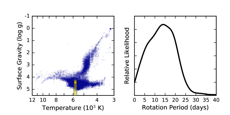
These cuts provide us with a total of 4876 stars. We additionally remove all stars that fall within 10 pixels of the detector edge, which would complicate aperture photometry calculations. We then select a similar number of stars with the same stellar parameter cuts, but no detected rotation periods to use as a control sample. These stars have similar colors and brightnesses, but are older, less active, and possibly evolved, so we should expect to see less variability in these stars. Differences between these two samples ensure that our observations are dominated by astrophysical information rather than underlying, unknown instrumental systematics. Once we have a list of KIC identifiers associated with the stars in the sample, we can perform photometry on each of these to search for long-term brightness variations.
2.2 Full Frame Images
2.2.1 Data Collection
The observations in this paper are taken from the 53 FFIs collected by Kepler during its primary mission. These data represent the only publicly available data of simultaneous observations of the entire Kepler field of view. Eight FFIs, called the “Golden FFIs,” were obtained over 34 hours during commissioning of the spacecraft before the start of the primary mission. Additional FFIs were obtained approximately once per month during the primary mission, immediately before the spacecraft turned towards Earth to transmit data. Two of these observations were missed because the spacecraft entered a safe mode state before data downlink. Additionally, on two occasions two FFIs were collected in succession. In one case the telescope was mispointed by 15 arcseconds, or approximately four pixels. We do not include this image in our analysis. On the second occasion, two acceptable images were obtained.
Each year during the primary mission, Kepler rolled by 90 degrees four times in order to keep its solar panels pointed at the Sun. The pointing is stable so that, after four rolls, each star falls back on the original pixel. As a result, the centroid of each star falls on four different pixels over the mission, each with its own unknown response function. The data from these four orientations can and should be treated as four different sets of observations, each with its own noise properties and potential systematics.
All FFIs are publicly available and contain observations of approximately 4.5 million objects in the telescope’s field of view. We downloaded all FFIs from the Mikulski Archive for Space Telescopes (MAST). Each image is already calibrated through a process similar to the Kepler pixel calibration pipeline (“CAL”), with the , dark , and smear estimated and corrected (Jenkins et al., 2010; Quintana et al., 2010).
2.2.2 Data Reduction
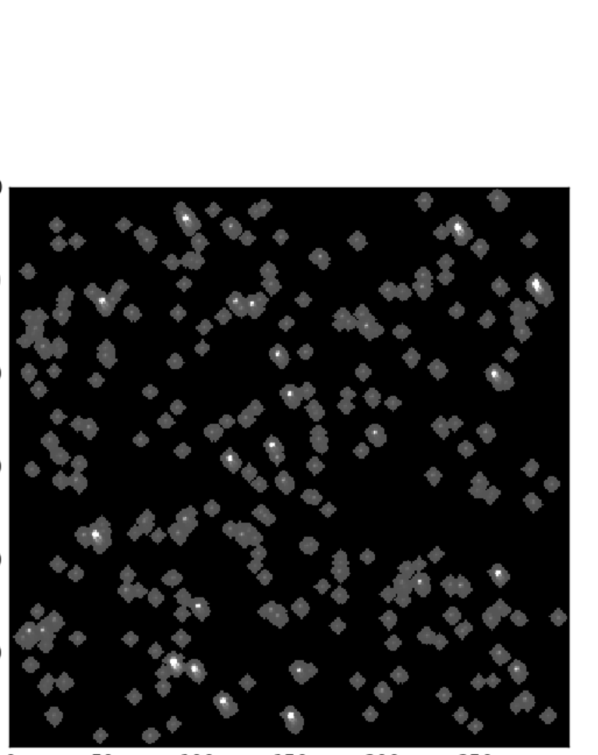
In this work, we develop time-series photometry for each of the target stars as described in Section 2.1. The method used is broadly similar to that of Montet & Simon (2016), but is more completely automated and achieves a typical precision higher than achieved by those authors by a factor of 2-3, depending on the target star and field. For all stars in our sample, we identify the row and column on the detector on which our target star appears, . We then select 300300 pixel (20 arcmin) “postcard” regions around each star (Fig. 2). In most cases, these regions are centered on the target star; when the target star falls near the edge of a detector they are shifted to ensure we always consider an equal-sized region. We build a master postcard for each field by summing over all 52 usable FFIs, allowing for shifts of up to one pixel in either direction to account for apparent pointing variations induced by differential velocity aberration (Haas et al., 2010). With this image, we identify the 250 brightest sources on the postcard corresponding roughly to stars brighter than 111This value depends on the density of stars in the field, which itself depends on the location of the star on the detector.. This selection will include our target star, while we draw our photometric comparison stars from the collection of other nearby stars that we select, typically around 200 in number.
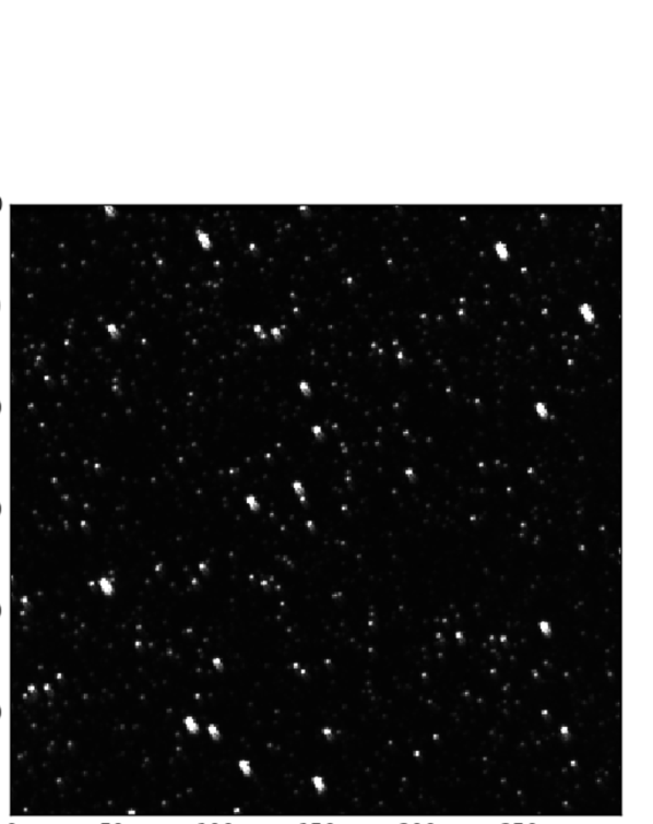
Once we have identified targets, the next step is to measure flux values for all targeted stars in each epoch. One possibility is to employ PSF modeling. Detailed PSF modeling is challenging with Kepler as the underlying flat field is poorly understood. PSF modeling has been shown to work for faint stars in crowded K2 fields, but underperforms simple aperture photometry for bright (), isolated stars (Libralato et al., 2016). We also explore model PSFs as the sum of three Gaussian functions, conditioned on all target stars in the postcard, but find that the uncertainties in the model fit are larger than those that we are able to achieve in simple aperture photometry. Therefore, we rely on aperture photometry in this work, leaving a detailed exploration of the possibility of PSF modeling for future efforts.
Aperture photometry requires accurate apertures that are large enough to capture the extent of the stellar PSF but small enough to only include the target star. To capture the Kepler PSF, the ideal aperture is asymmetric, especially near the edges of the detector (Bryson et al., 2010). Here, we use the computer vision library mahotas to draw appropriate apertures around our targets and separate them from the background (Coelho, 2013). We first choose all connected pixels with flux values larger than 1.5% of the brightest pixel’s flux, then extend the aperture to include a border of three pixels outside this region. In cases where multiple comparison stars have apertures that collide with each other, we combine their apertures into one and treat them as one single target.
We visually inspect each aperture for our science targets to ensure they contain only one star, manually removing stars with nearby, bright companions that encroach on the primary star’s PSF: due to the large PSFs on the detector, this removes approximately 10% of all possible stars from our analysis. Once our apertures are determined, we measure fluxes for all stars by summing over all pixels in each aperture.
For all stars, we notice a slow decrease in the observed flux. the magnitude of this decrease (Figure 3). Therefore, we consider all stars to potentially acceptable reference stars.
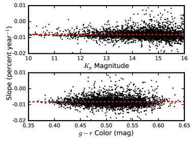
We invoke two methods to use the reference stars to measure the true long-term photometric behavior of each of our target stars. As a first pass, we simply eliminate all possible reference stars with excess variability ( from the mean) in more than 10% of frames. This should ensure intrinsically variable stars and stars with poorly drawn apertures are removed from the sample of reference stars. For all images in a particular orientation, we then sum the flux of all reference stars and divide the observed flux from our target star by this value. We divide each observed flux value by the median flux value for the target star from all epochs in that orientation, effectively eliminating possible effects caused by variations in the flat field between detectors used at different orientations. This method is fast and enables us to quickly measure the brightness of each star to look for candidate active stars.
For each of the candidate active stars, we then employ a probabilistic approach—similar in spirit to the “ubercalibration” method used in the Sloan Digital Sky Survey pipeline (Padmanabhan et al., 2008)—which enables us to measure the brightness of our target star and estimate an uncertainty on each observation. The full details of this method are given in Appendix A, but we summarize the important points here. We model the observed light curves of an ensemble of stars as noisy measurements of intrinsically variable time series observed with varying pixel responses and photometric zero points. We make this model tractable by assuming that nearby stars with similar properties sample a constant photometric zero point and that the pixel response for a particular source is constant in each season of observation. We fit for a distribution of zero points for each exposure, and the pixel responses and amplitude of intrinsic variability for each target by maximizing the likelihood function defined by this model (Equation A5). We use this maximum likelihood model to compute the de-trended light curve and its uncertainties.
The end result is time series photometry for all of our target stars, conditioned on the observations of nearby reference stars on the detector, with underlying systematics between detectors accounted for. These light curves are considerably more sparsely sampled than Kepler’s long cadence data, but allow for long-term trends which are overwhelmed by instrumental systematics in the long cadence data to be recovered. We make the code underlying FFI photometry code publicly available for community use and additional development as the f3 (Full Frame Fotometry) package222https://github.com/benmontet/f3.
2.2.3 Potential systematics
While they do enable accurate measurements of long-term flux variations on target stars in the field of view, FFI photmetry also comes with its own set of systematics. Many of these are familiar to users of Kepler and K2 data products, although they can manifest themselves in ways that may not be familiar. We show examples of each of these systematics in Fig. 4.
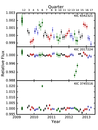
The most common systematic is a Sudden Pixel Sensitivity Dropout (SPSD). In these events, a cosmic ray hit causes a particular pixel to immediately decrease in sensitivity, leading to a decrease in the observed flux on that pixel without changing its neighbors (Smith et al., 2012). Pixels inflicted with SPSDs may recover after hours or days, while others remain degraded through the remainder of the mission.
SPSDs are visible in Kepler long cadence light curves of many stars. Since larger apertures are required to ensure accurate FFI photometry, there are more possibilities to have pixels affected by an SPSD than in typical Kepler data. SPSDs can be separated from true astrophysical variability in the FFIs because changes will manifest themselves in only one of the four telescope orientations, while the others will appear unchanged. Difficulties remain in separating astrophysical variability in the first or last quarter of observations from instrumental effects: this is especially true for the start of the mission, as the “Golden FFIs” are separated from the first FFI in the primary mission by 115 days.
The second most common systematic is apparent brightness variations caused by changes in the position of the star over the underlying unknown flat field. K2 observations have shown that there are significant interpixel and intrapixel variations in the flat field across the detector (Van Cleve et al., 2016). Some stars in the Kepler field of view can have proper motions as large as 0.1 pixels year-1, and differential velocity aberrations can cause periodic motions at the pixel level. Flat field variations can then manifest themselves as a long-term trend or periodic behavior with a period equal to that of the Kepler telescope, corresponding to each of those causes. The position of the star on each pixel at the start of the mission is effectively random, and the flat field between each orientation is different, so these can be separated from astrophysical variability: if the effect is instrumental, the variations look different in each of the four orientations and are correlated with the position of the star on the detector.
Additionally, cosmic rays can occasionally cause short brightness increases on a single pixel in a single FFI. Like SPSDs, these are somewhat more common than are seen in typical long cadence light curves since we require more pixels in each aperture. However, as these typically only affect a single FFI, while brightness variations from stellar activity manifest themselves on longer timescales, they generally do not affect our results significantly.
We visually inspect each of our light curves for each of these effects. We calculate the centroids of light in each of our apertures manually, summing the observed flux in each pixel. As we also verify there is not significant background contamination in our apertures, we do not expect any significant dilution due to a large number of high proper motion background or foreground stars significantly biasing our results.
2.3 Information from long cadence light curves
All of the stars in our target sample have measured rotation periods, so by definition they are also observed at long cadence in the Kepler mission. We use this information both to improve our photometry and to gain extra information in our analysis beyond a measurement of stellar rotation periods.
First, we use the Pre-search Data Conditioning (PDC) versions of the Kepler light curves (Stumpe et al., 2012) to apply a correction to the observed FFI photometry for the distribution of starspots at the time of the observation. Each FFI gives us an instantaneous observation of the brightness of the star, but as we know the time of the observation we can infer from the long cadence light curve whether that star is in a particularly bright or dim orientation due to the instantaneous distribution of starspots. By comparing the PDC light curve at the last long cadence observation of each month, one hour before the FFI observation, compared to the average flux value for that quarter, we can correct effects caused by one or a small number of starspots that may cause an aliasing effect with the monthly FFI cadence. We produce light curves with and without this correction to ensure that we do not induce any false signals of our own with this correction. Unfortunately, the vast majority of our reference stars do not have long cadence photometry, so we do not have the information to build a global solution that accounts for starspots on all reference stars. Instead, we reject variable stars as references, as described in Section 2.2.2.
We also use the long cadence light curve to look for changes in the starspot distribution in time. A long-term change in the observed variance due to starspots would suggest additional evidence of magnetic cycles (Mathur et al., 2014; Estrela & Valio, 2016). A correlation or anti-correlation between the observed brightness of the star in the FFI photometry and variability from starspots would suggest that the brightness variations are dominated by faculae or starspots, respectively (Radick et al., 1998).
As a proxy for starspot variability, we calculate the metric from the long cadence data. measures a running standard deviation of points within five rotation periods of each cadence, and has been shown to be a useful tracer of magnetic activity variations that requires only photometry (Mathur et al., 2014). We then compare this photometric activity index, , to the observed bulk brightness variations to separate .
3 Results
Of the total of 3,845 stars targeted in this survey, we find that 463 of them have observed brightness variations over the Kepler mission. Of course, this does not mean that the remainder are unvarying: their variability is either too small in amplitude or too low in frequency to be observed over the four-year baseline of Kepler’s FFIs. The stars with observed photometric variability are listed in Table 1, and a representative sample of observed variability is shown in Figure 5.
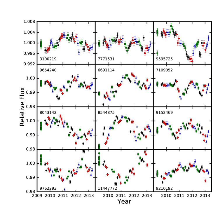
In almost all cases, we neglect stars with long-term trends in the photometry, only considering stars with non-linear variability over the Kepler mission. This is due to the possibility that long-term trends could be affected by data artifacts and non-astrophysical events, as discussed in Section 4.4. We claim any other observed variability is intrinsic to the star and related to modulations in the overall stellar brightness induced by magnetic activity. In the following subsection, we attempt to rule out other explanations.
| KIC ID | Rotation PeriodaaTaken from McQuillan et al. (2014). | bbTaken from Brown et al. (2011). | colorccTaken from Everett et al. (2012). | ScatterddStandard deviation of the photometry, taking the Golden FFIs as a single point. This estimate includes photometric uncertainty and scatter from intrinsic stellar variability together. | Variability | Notes |
|---|---|---|---|---|---|---|
| (days) | (mag) | (mag) | (ppt) | |||
| 2013503 | 19.065 | 13.759 | 0.701 | 6.62 | Spots | |
| 2447723 | 23.023 | 13.052 | 0.649 | 2.29 | Spots | |
| 2581014 | 16.418 | 13.620 | 0.678 | 0.92 | Spots | |
| 2582166 | 20.659 | 12.606 | 0.647 | 0.99 | Faculae | |
| 2694675 | 12.65 | 14.335 | 0.689 | 3.77 | Spots | 3 |
| 2694810 | 0.478 | 12.980 | 0.645 | 6.13 | 1,2,3 | |
| 2712799 | 8.567 | 15.138 | 0.587 | 4.89 | Spots | |
| 2720200 | 10.846 | 14.882 | 0.697 | 6.83 | Spots | |
| 2848223 | 4.751 | 13.620 | — | 6.32 | Spots | |
| 2974459 | 48.867 | 12.476 | 0.641 | 1.26 | Faculae |
Note. — Table 1 will be published in its entirety in machine-readable format on the journal website. A portion is reproduced here as a guide for formatting. A version is also available in the source materials for this manuscript on the arXiv.
3.1 Alternative Explanations
If the observed long-term variability were the result of an instrumental effect, then we should expect to see similar behavior on all stars with similar stellar properties. Fortunately, a control sample exists to test this idea. In addition to the stars with measured rotation periods observed by McQuillan et al. (2014), the authors of that paper also published a list of stars without measured rotation periods. We select a sample of 3,000 stars that satisfy our same temperature and surface gravity cuts, but have no measured rotation signal.
These stars, having similar magnitudes and colors as our target sample, should provide a reasonable control sample to compare against in a search for instrumental effects. We repeat our analysis on this control sample and search for photometric variability. We find only eleven of the stars have observed variability, significantly lower than the rate observed in the target sample. Of these, closer inspection reveals three stars’ (KIC 3338794, 4639329, and 4649300) light curves do indeed exhibit a rotation signature in some quarters, but the signal was not detected in enough segments of the data to be included as a bona fide detection by McQuillan et al. (2014). If we assume these rotation signals are real, then we have only eight stars with FFI variability but no rotation signature, suggesting that the vast majority of our observed signals are not instrumental in nature.
Astrophysically, the control sample is not necessarily identical to the target sample, despite their similar inferred temperature and gravity. As they do not have observed rotation periods, they are likely on average to be less chromospherically active and older. A fraction of them may be nearly pole-on, while others may be slightly evolved relative to their counterparts with measured rotation, leading to their rotation signals being removed by the Kepler data processing pipeline.
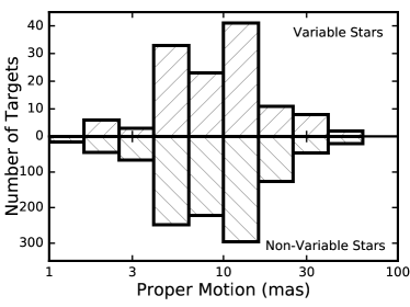
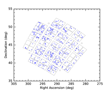
If the stars in the control sample are systematically more distant, then they might systematically have lower proper motions. Therefore, if the observed variability were caused by stars passing behind small-scale structure in the ISM, changing the extinction along our line of sight and modulating the brightness (Meyer & Blades, 1996), then we might expect to not observe as much variability in the control sample. This scenario is not well represented by the data either. In this case, we would expect stars with higher proper motion to have higher rates of variability, which is not the case, as shown in Figure 6. Moreover, we would expect stars near the galactic plane, where extinction is higher, to preferentially display variability, while we detect signals across the Kepler field (Figure 7).
We also note that stars with observed variability are more likely to be detected in the GALEX survey of the Kepler field, which has a limiting NUV magnitude of 22.6 (Olmedo et al., 2015). Of the 463 target stars, 145 of them (31.3%) are detected in the UV. Of the other 3,382 stars in our sample, 775 of them (22.9%) are detected in the UV, a discrepancy. This is in line with expectations, as UV-bright stars are more likely to be chromospherically active (Findeisen et al., 2011).
These tests rule out certain alternate explanations for the observed long-term variability, but do not prove that the brightness variations we are observing are magnetic in nature. The strongest evidence in favor of that explanation is through comparing the observed variability to other tracers of magnetic activity, such as starspots.
3.2 Photometry as tracer of magnetic activity
Kepler long cadence photometry can provide information on the evolution of starspots, a proxy of magnetic activity. Changes in the level of starspot variability have been shown to correlate with spectroscopic proxies of stellar activity (Mathur et al., 2014; Salabert et al., 2016b). Starspot variability has been shown to correlate with long-term brightness variations recently, C. Karoff et al. (submitted) have shown that brightness variations observed through Kepler FFI photometry also correlate with spectroscopic and photometric proxies of magnetic activity for KIC 8006161.
Here, we do not have uniform spectroscopy for our target stars, but we do have uniform long cadence photometry: as these stars are selected from their rotation properties, they all by definition are on silicon during the Kepler mission. We compare the FFI photometry to the index for each of our stars with non-constant flux over the mission. We find that 84% of stars exhibit behavior in their long-term brightness that corresponds to the variability observed in the index. We label each star’s brightness fluctuations as either correlated or anti-correlated in time with the index, The majority (68%) are anticorrelated: increases in spot activity correspond to an overall decrease in brightness. This is the opposite as observed in the Sun (Noyes et al., 1984).
3.3 A Transition in the Stellar Dynamo
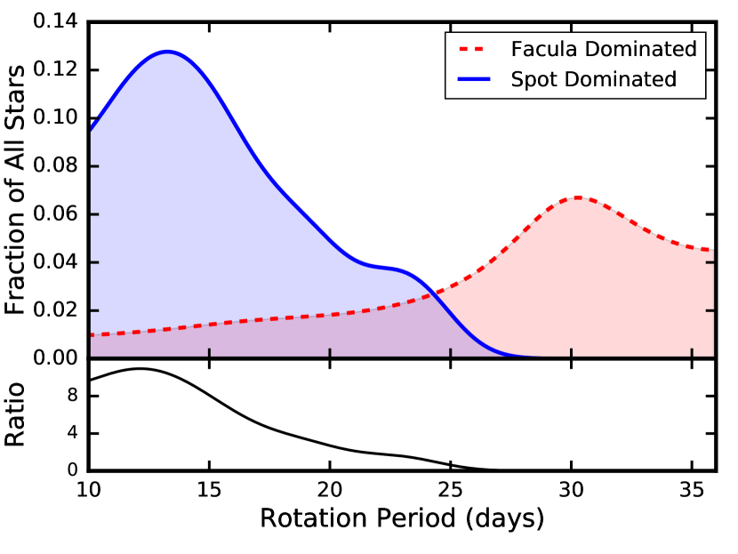
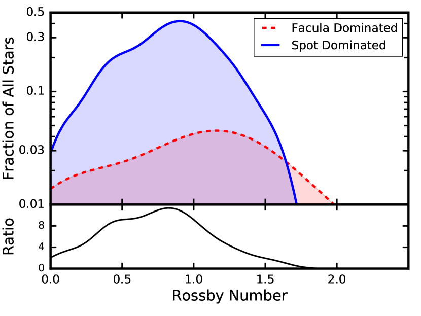
While the majority of stars have brightness variations anticorrelated with their starspots, this is not true at all rotation periods. This is the case because the majority of stars in our sample have rotation periods considerably shorter than the Sun’s. Fig. 8 shows this effect. At rotation periods between 10 and 15 days, 11 percent of stars show detectability over the four years of Kepler observations; spot-dominated, anticorrelated variability is an order of magnitude more common here than facula-dominated, correlated variability. However, at a rotation period of 15 days, the occurrence of spot-dominated variability sharply decreases and facula-dominated variability rises, We do not detect any stars with spot-dominated variability with rotation periods beyond 26 days, while detectable facula-dominated variability continues to be increasingly common at rotation periods slower than the Sun.
We can convert observed stellar parameters into Rossby numbers (), following the prescription of Noyes et al. (1984) who relate a star’s color to its convective turnover time. We use the colors of Everett et al. (2012), who performed a UBV survey of the Kepler field largely complete to . The typical uncertainty in each bandpass is 0.02 mag, leading to an uncertainty of 0.03 mag in the color and therefore days in the convective turnover time. We see the same result in this space: stars with lower values of are considerably more likely to have spot-dominated variability, while no stars with are spot-dominated. For reference, the Sun has based on its color and rotation period.
Rotation period correlates with stellar age (Barnes, 2007). Mamajek & Hillenbrand (2008) have shown that for main-sequence stars, the two are related such that
| (1) |
where is the color of the star in the Johnson-Cousins filters, the star’s age in Myr, the rotation period of the star in days, and , , , and constants such that , , , and . For the Sun, (Ramírez et al., 2012). The stars in our sample have values approximately normally distributed with mean of 0.64 and standard deviation 0.04. In this case, Equation 1 reduces to
| (2) |
Therefore, the peak occurrence of detectable spot-dominated variability occurs at an age of approximately 1200 Myr, and begins to fall off significantly at an age of 1600 Myr. and we do not detect any stars with spot-dominated variability older than 4200 Myr.
4 Discussion
4.1 Transition or two populations?
Understanding this putative transition means understanding the stars in our sample. One help would be additional observations: it is possible that 13% of stars with a rotation period of 13 days have observable spot-dominated variability, or it is possible that all such stars have a signal, but it is only detectable over a four-year time baseline when viewed from a random angle 13% of the time. Continued photometric observations at this cadence and precision would be helpful, and will be obtained as described in Section 5.2.
Upcoming parallax observations from Gaia will also be important for characterizing these systems. The photometric-based effective temperature estimates for our stars have uncertainties similar in magnitude to the range of temperatures chosen, suggesting our Sun-like stars span the F7 to G4 spectral classes. This cut will affect different rotation periods differently. The sample of stars with rotation periods of days likely includes a higher fraction of F stars, which slow down more slowly and have a shorter main sequence lifetime; the sample at a rotation period of days will have a larger fraction of mid-G stars. As stated in the previous section, we do not detect any stars with spot-dominated variability older than 4200 Myr; this sample by definition cannot contain stars with main sequence lifetimes shorter than 4200 Myr. A more detailed characterization of individual systems and the evolution of the stellar dynamo of G2 stars in particular will require improved stellar parameters, which will become more attainable with measured parallaxes to these stars.
In this work, we take the gyrochronological relations at face value in our analysis that the transition between spot-dominated and facula-dominated variability occurs at an age younger than the Sun. Comparisons to solar twins at similar ages to the Sun show the Sun’s rotation period to be typical (dos Santos et al., 2016). Recently, van Saders et al. (2016) have shown older stars can have significantly weakened magnetic braking compared to younger stars, leading to a discrepancy between rotation periods and age estimates, especially for stars more evolved than the Sun.
As the vast majority of stars in our sample have ages younger than the Sun, and the transition of interest occurs at rotation periods faster than the Sun, it is likely our results are not significantly affected by this discrepancy, although it is certainly possible that some of our stars are affected. Where possible, asteroseismic ages for stars in our sample with observed variability would be useful. As the Kepler telescope is no longer able to point at the Kepler field and these measurements require short cadence data, additional data is likely needed for the vast majority of our sample in order for such an analysis to come to fruition. In the meantime, spectroscopic activity indicators would be useful to probe the putative transition and compare to the spectroscopic transition considered by previous studies, such as that of Metcalfe et al. (2016).
4.2 Comparison with previous work
Metcalfe et al. (2016) have suggested spectroscopic diagnostics indicate that the solar dynamo may be in transition, due to the loss of the large-scale stellar magnetic field. Although we find a possible transition at a younger age, around 3 Gyr, these two results are not necessarily inconsistent. The transition described in that paper, which matches the theoretical work of van Saders et al. (2016), would suggest that weakened magnetic braking in older stars would lead to a pileup of rotation periods as a function of spectral type. If the collection of spot-dominated stars we observe with rotation periods of days were mostly late F stars at a variety of ages, and the facula-dominated stars with rotation periods of 25 days were mostly G stars, then this would support these predictions. As before, improved stellar properties and ages would be useful to better understand the relation between the potential transition discussed here and the spectroscopic transition discussed in that paper.
Oláh et al. (2016) found that there is a transition between smooth and complex magnetic cycles at an age of 2 to 3 Gyr of age. This is in line with our analysis, as we find a rapid decrease in the fraction of stars with spot dominated variability during this age rage, which corresponds to rotation periods of 17-22 days. It is plausible that the more rapidly rotating, spot-dominated stars contain short-period and long-period cycles (e.g Brandenburg et al., 2017), leading to a more complex appearance in ground-based data. Additional long-term observations of these stars, leading to a detection of longer-timescale magnetic cycles in these same stars, would support this claim.
Saar & Brandenburg (1999) and Böhm-Vitense (2007) divide stars with observed cycles into “active” and “inactive” branches. Some of these stars have cycles that would be observable over the relatively short time baseline of Kepler. These shorter cycle periods are limited by observational biases from the ground and are not well-sampled. Data from Kepler provide an opportunity to identify systems to compare to the ground-based detections of magnetic cycles along both of these branches.
4.3 Particularly Interesting Systems
4.3.1 Possibly Complete Magnetic Cycles
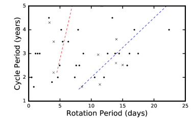
A four-year time baseline does not preclude the detection of magnetic cycles. Previous studies have shown the existence of magnetic cycles lasting 2-3 years on stars (e.g. Saar & Brandenburg, 1999). We identify by eye 28 systems which appear to exhibit at least one cycle over the baseline of Kepler. Brandenburg et al. (2017) have shown stars with longer cycles can have additional, shorter cycles with periods of 1-3 years. Therefore, it is not implausible that some of our stars may have considerably longer cycles in addition to the ones observed in Kepler FFI photometry which will reveal themselves through continued observations.
The observed cycles and rotation periods for these stars are plotted in Fig. 9, as well as similar stars in the literature. We see that many of these stars follow the “active” and “inactive” branches of Böhm-Vitense (2007).
Additional photometry of these stars to confirm these cycles, and search for longer cycles that are also possibly present in these stars can provide constraints for future models of stellar dynamos. In Table 2 we list those systems observed to have apparently complete magnetic cycles, with an estimate of the observed cycle period. Two of these stars, each with very short periods and likely binary systems, have their cycles noted in the index but not in the FFI data, suggesting the cycle may be on the fainter component which does not dominate the FFI photometry. These two stars are noted in the Table. Additional observations of these systems could help understand the evolution of magnetic cycles of binary systems.
| KIC ID | Semiamplitude | Period |
|---|---|---|
| (percent) | (yr) | |
| 2694810 | 0.6 | 2 |
| 3236788 | 2.0 | 3.5 |
| 3743810 | 0.3 | 3 |
| 4555566 | 1.2 | 2 |
| 4726114 | 0.3 | 4 |
| 5352687 | 0.9 | 4 |
| 5450764 | 0.7 | 4 |
| 6038355 | 0.8 | 2.5 |
| 6263983 | 1.0 | 3 |
| 6708110 | 1.2 | 3 |
| 7272437 | 0.1 | 3 |
| 7432092 | 0.3 | 4 |
| 7433192 | 0.2 | 3 |
| 7678238 | 0.6 | 2.5 |
| 8041424 | 1.8 | 1.8 |
| 8043142 | 0.5 | 4.5 |
| 8345997 | 0.4 | 3 |
| 8759594 | 0.2 | 2.5 |
| 8804069 | 0.9 | 3 |
| 930627111Short period binary | — | 1.6 |
| 10087863 | 0.6 | 3 |
| 10122937 | 0.9 | 3.5 |
| 1092124211Cycle observed and period inferred from variability | — | 3 |
| 11014223 | 1.5 | 2 |
| 11033434 | 0.6 | 2 |
| 11415049 | 0.3 | 2 |
| 11873617 | 0.7 | 2.5 |
| 12417799 | 1.2 | 4.5 |
4.3.2 Short-Period Binaries
Several of the stars observed with the most extreme long-term brightness variations have, on inspection of their long cadence light curves, been revealed as short-period eclipsing binaries. It has long been considered that contact binaries could have extreme magnetic activity which leads to an evolution of their brightness (Applegate, 1992). Such brightness variations have been detected, as has indirect evidence for short period magnetic cycles on contact biaries (Ibanoǧlu et al., 2001; Borkovits et al., 2005).
Recently, Marsh et al. (2017) analyzed nearly 10,000 contact binaries observed in the Catalina Real-Time Transient Survey (Djorgovski et al., 2011), finding that 20% of them undergo a linear change in brightness during the survey.
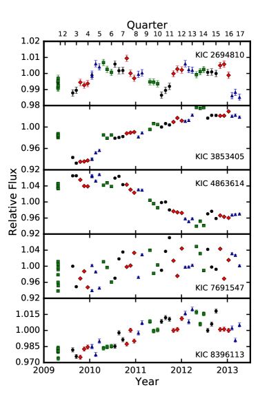
Here, we present an additional five short-period binaries with long-term FFI variability. A detailed analysis of their evolution is beyond the scope of this work, but we present their light curves in Fig. 10 as a potential avenue for further follow-up observations. In general, the detailed long cadence light curves from Kepler enable the opportunity to characterize both the evolution in the eclipse-to-eclipse variability over the mission in concert with long-term photometric variability.
While the changes in brightness for contact binaries have been traditionally considered to be due to magnetic effects, other effects can cause long-term photometric trends in the observed photometry as well.
4.4 Long-Term Photometric Trends
In this work, we largely ignore systems with long-term trends observed in the Kepler FFI photometry. While we can eliminate most false positives for other stars with variability, meaning the results in Table 1 should be dominated by stars with magnetic activity variations, some false positives remain for systems with long-term trends. One false positive that may be common is faint stars in the field of view. The typical Kepler PSF has a radius of 6 arcsec (Bryson et al., 2010); the Kepler Input Catalog only includes targets down to 21st magnitude and is incomplete at the faint end (Brown et al., 2011).
A faint M dwarf with a high proper motion could then be found to be expanding its PSF into the aperture for any target, leading to a long-term trend in the data. With the current data, we are unable to test this. Detailed PSF modeling of each star may be able to improve this in the future: if certain stars have changing levels of contamination, then their PSF should be slightly varying relative to other nearby stars.
In some cases, long-term trends can also be caused by varying levels of extinction. This may be especially true for contact binaries or stars near the end of their life cycles, where shells of ejected material are expanding and decreasing in opacity in time. KIC 3853405 is an example of a system that displays this behavior. This contact binary increases in brightness by more than 5% over the Kepler mission (Fig. 10). While described in the previous subsection as potential magnetic variability, the variation could also be explained by a change in the opacity of circumstellar dust ejected in a recent outburst or by an actual increase in luminosity as the two stellar cores prepare to merge (Tylenda et al., 2011; Molnar et al., 2017). Detailed modeling of both the long cadence light curves and FFI photometry, combined with additional follow-up observations could be used to better understand this system, but is beyond the scope of this paper.
In Table 1 and throughout this work, we reject nearly all systems with long-term trends as they cannot be uniquely shown to be related to changes of the magnetic activity of the stars. The only exceptions are stars in which the index is also changing in a linear way throughout the Kepler mission. As the apertures used in long cadence photometry are substantially smaller than ours, we do not necessarily expect FFI brightness variations from stellar contamination to dilute the long cadence light curves in the same way, so we argue these changes are likely to be astrophysical. We specifically note these systems in Table 1, and also note their inclusion or exclusion does not significantly affect the results of our analysis.
5 Conclusions
5.1 FFIs as a probe of long-term astrophysical variability
In this paper, we have presented the method behind the f3 package to produce very long cadence light curves from Kepler FFI data. These light curves provide photometry at monthly cadence at 52 epochs across the Kepler mission, and generally avoid the removal of astrophysical variations on month-long or slower timescales inherent in the Kepler long cadence data.
Accurate relative photometry on long time scales is important, as it can be used to probe long-term behavior of the brightness of astrophysical objects typically removed in transit surveys like Kepler. Here we develop light curves for a sample of Sun-like stars with observed rotation periods to probe changes in stellar activity in time, finding that we do observe evidence for magnetic activity in a substantial fraction of Sun-like stars, especially those that are young and rapidly rotating. We find that there appears to be a transition in the stellar dynamo at a stellar rotation period of 15-25 days, corresponding to a gyrochronological age of 1.5-3.5 Gyr, although this may reflect a change in stellar parameters, with younger, hotter stars in our sample more likely to be rapidly rotating than older, cooler stars. Stars with rotation periods faster than 15 days have photometric variations that are typically dominated by starspots, while more slowly rotating stars have variations dominated by faculae. Additionally, we find that the more rapidly rotating stars are typically significantly more active than the slowly rotating stars, in line with previous work. We also identify 28 stars with apparently complete short-period magnetic cycles, finding they are consistent with the “active” and “inactive” branches of stars of Saar & Brandenburg (1999).
Although it is our application in this work, this method is not exclusive to observing magnetic cycles. In principle, photometry from f3 could be used to probe intrinsic brightness variations from variable stars, variable extinction through the ISM, or evolution of binary stars or evolved stars which affects their observed brightness. To explore this dataset to the fullest extent possible, we make our code publicly available for community use and development.
5.2 Future prospects
Future missions will enable similar measurements on even larger samples of stars. TESS (Ricker et al., 2014) will obtain a FFI every minutes, enabling aperture photometry with a large number of reference stars at a high cadence. However, each field will only be observed for one month at a time, and the continuous viewing zone will only span one year of observations: longer time baselines will only be possible with an extended mission. Stars in the continuous viewing zone will fall on 13 different pixels for one month each during the mission, so long-term changes like those observed in this field will require detailed knowledge of the instrument’s flat field. We encourage the TESS team to make every effort to understand the flat field both before launch and during the mission.
Another possibility to detect magnetic cycles on a large number of stars is provided by the Gaia mission (Gaia Collaboration et al., 2016). While its photometric performance is often overlooked relative to its astrometric potential, Gaia will return mmag photometry for all stars with and mmag photometry for all stars with (Jordi et al., 2010). With the typical star observed 70 times over 10 years, Gaia will provide FFI-like photometry at FFI-like cadence for millions of stars for a decade. Gaia long-term photometry combined with rotation periods from simultaneous observations with K2, TESS, and possibly PLATO (Rauer et al., 2014) will enable detailed photometric studies of magnetic cycles for millions of stars across the galaxy, allowing us to understand the interplay between magnetic activity and photometric modulations across the H-R diagram.
Appendix A Probabilistic calibration model
We model the relative flux of star at time as
| (A1) |
where the hat indicates this is the predicted model value of , is the total response of the pixels in the aperture for the star at the season of exposure , and is the time-variable mean zero point of exposure .
To capture these effects, we model the variance for each observation as
| (A2) |
where is the amplitude of the intrinsic variability of star , is the scatter in the zero point of the exposure , and is photometric noise level. To break the degeneracy between the pixel responses and the zero points, we regularize the fit by selecting Gaussian priors with unit mean and variance for both and .
The model described in the previous paragraph assumes that the measurements in the light curve are independent. Since the observations are not uniformly distributed in time, this can lead to biased estimates of the pixel responses for targets with long-term variability—exactly the case that we are interested in. To mitigate this issue, we model the true flux of the target star using a Gaussian Process with a Matérn-3/2 kernel. This implies a log-likelihood function for the target star of
| (A3) |
where we have labeled the target star with and the elements of the covariance matrix are given by
| (A4) |
where is the Kronecker delta, is the number of cadences in the light curve, and and are parameters of the model.
Applying this model to a target star (labeled ) and set of reference stars observed at cadences, we obtain the log-likelihood function
| (A5) | |||||
where refers to the set of the following parameters:
-
•
parameters ,
-
•
parameters ,
-
•
parameters ,
-
•
parameters ,
-
•
a single noise parameter , and
-
•
the 2 hyperparameters of the Gaussian Process, and .
To fit for the maximum likelihood parameters , we build this model using Theano (Theano Development Team, 2016) and maximize Equation (A5) using 2000 iterations of the Adam algorithm (Kingma & Ba, 2014).
Conditioned on these maximum likelihood parameters, the de-trended flux for star at time is given by
| (A6) |
with predictive variance
| (A7) |
References
- Angus et al. (2015) Angus, R., Aigrain, S., Foreman-Mackey, D., & McQuillan, A. 2015, MNRAS, 450, 1787
- Applegate (1992) Applegate, J. H. 1992, ApJ, 385, 621
- Baliunas et al. (1995) Baliunas, S. L., Donahue, R. A., Soon, W. H., et al. 1995, ApJ, 438, 269
- Barnes (2007) Barnes, S. A. 2007, ApJ, 669, 1167
- Bastien et al. (2016) Bastien, F. A., Stassun, K. G., Basri, G., & Pepper, J. 2016, ApJ, 818, 43
- Böhm-Vitense (2007) Böhm-Vitense, E. 2007, ApJ, 657, 486
- Borkovits et al. (2005) Borkovits, T., Elkhateeb, M. M., Csizmadia, S., et al. 2005, A&A, 441, 1087
- Borucki et al. (2010) Borucki, W. J., Koch, D., Basri, G., et al. 2010, Science, 327, 977
- Brandenburg et al. (2017) Brandenburg, A., Mathur, S., & Metcalfe, T. S. 2017, ArXiv e-prints, arXiv:1704.09009
- Brown et al. (2011) Brown, T. M., Latham, D. W., Everett, M. E., & Esquerdo, G. A. 2011, AJ, 142, 112
- Bryson et al. (2010) Bryson, S. T., Tenenbaum, P., Jenkins, J. M., et al. 2010, ApJ, 713, L97
- Charbonneau (2010) Charbonneau, P. 2010, Living Reviews in Solar Physics, 7, 3
- Coelho (2013) Coelho, L. P. 2013, Journal of Open Research Software, 1, doi:10.5334/jors.ac. http://dx.doi.org/10.5334/jors.ac
- Davenport (2016) Davenport, J. R. A. 2016, ApJ, 829, 23
- De Cat et al. (2015) De Cat, P., Fu, J. N., Ren, A. B., et al. 2015, ApJS, 220, 19
- Djorgovski et al. (2011) Djorgovski, S. G., Drake, A. J., Mahabal, A. A., et al. 2011, ArXiv e-prints, arXiv:1102.5004
- dos Santos et al. (2016) dos Santos, L. A., Meléndez, J., do Nascimento, J.-D., et al. 2016, A&A, 592, A156
- Egeland et al. (2015) Egeland, R., Metcalfe, T. S., Hall, J. C., & Henry, G. W. 2015, ApJ, 812, 12
- Endl et al. (2016) Endl, M., Brugamyer, E. J., Cochran, W. D., et al. 2016, ApJ, 818, 34
- Estrela & Valio (2016) Estrela, R., & Valio, A. 2016, ApJ, 831, 57
- Everett et al. (2012) Everett, M. E., Howell, S. B., & Kinemuchi, K. 2012, PASP, 124, 316
- Findeisen et al. (2011) Findeisen, K., Hillenbrand, L., & Soderblom, D. 2011, AJ, 142, 23
- Fossati et al. (2017) Fossati, L., Marcelja, S. E., Staab, D., et al. 2017, ArXiv e-prints, arXiv:1702.02883
- Fröhlich & Lean (1998) Fröhlich, C., & Lean, J. 1998, Geophys. Res. Lett., 25, 4377
- Fröhlich & Lean (2004) —. 2004, A&A Rev., 12, 273
- Gaia Collaboration et al. (2016) Gaia Collaboration, Prusti, T., de Bruijne, J. H. J., et al. 2016, A&A, 595, A1
- Gaidos et al. (2016) Gaidos, E., Mann, A. W., & Ansdell, M. 2016, ApJ, 817, 50
- Galilei et al. (1613) Galilei, G., Welser, M., & de Filiis, A. 1613, Istoria E dimostrazioni intorno alle macchie solari E loro accidenti comprese in tre lettere scritte all’illvstrissimo signor Marco Velseri …
- García et al. (2010) García, R. A., Mathur, S., Salabert, D., et al. 2010, Science, 329, 1032
- Gilliland et al. (2010) Gilliland, R. L., Brown, T. M., Christensen-Dalsgaard, J., et al. 2010, PASP, 122, 131
- Gilliland et al. (2011) Gilliland, R. L., Chaplin, W. J., Dunham, E. W., et al. 2011, ApJS, 197, 6
- Gosling (1993) Gosling, J. T. 1993, J. Geophys. Res., 98, 18937
- Guo et al. (2017) Guo, X., Johnson, J. A., Mann, A. W., et al. 2017, ApJ, 838, 25
- Haas et al. (2010) Haas, M. R., Batalha, N. M., Bryson, S. T., et al. 2010, ApJ, 713, L115
- Hall et al. (2009) Hall, J. C., Henry, G. W., Lockwood, G. W., Skiff, B. A., & Saar, S. H. 2009, AJ, 138, 312
- Hathaway (2015) Hathaway, D. H. 2015, Living Reviews in Solar Physics, 12, 4
- Hawley et al. (2014) Hawley, S. L., Davenport, J. R. A., Kowalski, A. F., et al. 2014, ApJ, 797, 121
- Huber et al. (2013) Huber, D., Carter, J. A., Barbieri, M., et al. 2013, Science, 342, 331
- Huber et al. (2014) Huber, D., Silva Aguirre, V., Matthews, J. M., et al. 2014, ApJS, 211, 2
- Hunter et al. (2007) Hunter, J. D., et al. 2007, Computing in science and engineering, 9, 90
- Ibanoǧlu et al. (2001) Ibanoǧlu, C., Evren, S., Taš, G., Devlen, A., & Çakïrlï, Ö. 2001, A&A, 371, 626
- Jenkins et al. (2010) Jenkins, J. M., Caldwell, D. A., Chandrasekaran, H., et al. 2010, ApJ, 713, L87
- Jenkins et al. (2015) Jenkins, J. M., Twicken, J. D., Batalha, N. M., et al. 2015, AJ, 150, 56
- Jordi et al. (2010) Jordi, C., Gebran, M., Carrasco, J. M., et al. 2010, A&A, 523, A48
- Kingma & Ba (2014) Kingma, D. P., & Ba, J. 2014, in Proceedings of the 3rd International Conference on Learning Representations (ICLR)
- Lehmann et al. (2012) Lehmann, H., Zechmeister, M., Dreizler, S., Schuh, S., & Kanzler, R. 2012, A&A, 541, A105
- Libralato et al. (2016) Libralato, M., Bedin, L. R., Nardiello, D., & Piotto, G. 2016, MNRAS, 456, 1137
- Lockwood et al. (1997) Lockwood, G. W., Skiff, B. A., & Radick, R. R. 1997, ApJ, 485, 789
- Luger et al. (2016) Luger, R., Agol, E., Kruse, E., et al. 2016, AJ, 152, 100
- Mamajek & Hillenbrand (2008) Mamajek, E. E., & Hillenbrand, L. A. 2008, ApJ, 687, 1264
- Marsh et al. (2017) Marsh, F. M., Prince, T. A., Mahabal, A. A., et al. 2017, MNRAS, 465, 4678
- Mathur et al. (2014) Mathur, S., García, R. A., Ballot, J., et al. 2014, A&A, 562, A124
- McQuillan et al. (2014) McQuillan, A., Mazeh, T., & Aigrain, S. 2014, ApJS, 211, 24
- Metcalfe et al. (2010) Metcalfe, T. S., Basu, S., Henry, T. J., et al. 2010, ApJ, 723, L213
- Metcalfe et al. (2016) Metcalfe, T. S., Egeland, R., & van Saders, J. 2016, ApJ, 826, L2
- Metcalfe et al. (2013) Metcalfe, T. S., Buccino, A. P., Brown, B. P., et al. 2013, ApJ, 763, L26
- Meyer & Blades (1996) Meyer, D. M., & Blades, J. C. 1996, ApJ, 464, L179
- Molnar et al. (2017) Molnar, L. A., Van Noord, D. M., Kinemuchi, K., et al. 2017, ApJ, 840, 1
- Montet & Simon (2016) Montet, B. T., & Simon, J. D. 2016, ApJ, 830, L39
- Mullally et al. (2016) Mullally, F., Barclay, T., & Barentsen, G. 2016, K2fov: Field of view software for NASA’s K2 mission, Astrophysics Source Code Library, , , ascl:1601.009
- Nielsen et al. (2013) Nielsen, M. B., Gizon, L., Schunker, H., & Karoff, C. 2013, A&A, 557, L10
- Noyes et al. (1984) Noyes, R. W., Hartmann, L. W., Baliunas, S. L., Duncan, D. K., & Vaughan, A. H. 1984, ApJ, 279, 763
- Oláh et al. (2016) Oláh, K., Kővári, Z., Petrovay, K., et al. 2016, A&A, 590, A133
- Olmedo et al. (2015) Olmedo, M., Lloyd, J., Mamajek, E. E., et al. 2015, ApJ, 813, 100
- Padmanabhan et al. (2008) Padmanabhan, N., Schlegel, D. J., Finkbeiner, D. P., et al. 2008, ApJ, 674, 1217
- Pinsonneault et al. (2012) Pinsonneault, M. H., An, D., Molenda-Żakowicz, J., et al. 2012, ApJS, 199, 30
- Quintana et al. (2010) Quintana, E. V., Jenkins, J. M., Clarke, B. D., et al. 2010, in Proc. SPIE, Vol. 7740, Software and Cyberinfrastructure for Astronomy, 77401X
- Radick et al. (1998) Radick, R. R., Lockwood, G. W., Skiff, B. A., & Baliunas, S. L. 1998, ApJS, 118, 239
- Ramírez et al. (2012) Ramírez, I., Michel, R., Sefako, R., et al. 2012, ApJ, 752, 5
- Rauer et al. (2014) Rauer, H., Catala, C., Aerts, C., et al. 2014, Experimental Astronomy, 38, 249
- Reinhold et al. (2017) Reinhold, T., Cameron, R. H., & Gizon, L. 2017, ArXiv e-prints, arXiv:1705.03312
- Ricker et al. (2014) Ricker, G. R., Winn, J. N., Vanderspek, R., et al. 2014, in Proc. SPIE, Vol. 9143, Space Telescopes and Instrumentation 2014: Optical, Infrared, and Millimeter Wave, 914320
- Saar & Brandenburg (1999) Saar, S. H., & Brandenburg, A. 1999, ApJ, 524, 295
- Salabert et al. (2016a) Salabert, D., Régulo, C., García, R. A., et al. 2016a, A&A, 589, A118
- Salabert et al. (2016b) Salabert, D., García, R. A., Beck, P. G., et al. 2016b, A&A, 596, A31
- Schwabe (1844) Schwabe, M. 1844, Astronomische Nachrichten, 21, 233
- Shapiro et al. (2014) Shapiro, A. I., Solanki, S. K., Krivova, N. A., et al. 2014, A&A, 569, A38
- Silva Aguirre et al. (2015) Silva Aguirre, V., Davies, G. R., Basu, S., et al. 2015, MNRAS, 452, 2127
- Smith et al. (2012) Smith, J. C., Stumpe, M. C., Van Cleve, J. E., et al. 2012, PASP, 124, 1000
- Soderblom (2010) Soderblom, D. R. 2010, ARA&A, 48, 581
- Stumpe et al. (2012) Stumpe, M. C., Smith, J. C., Van Cleve, J. E., et al. 2012, PASP, 124, 985
- Theano Development Team (2016) Theano Development Team. 2016, arXiv e-prints, abs/1605.02688. http://arxiv.org/abs/1605.02688
- Tregloan-Reed & Southworth (2013) Tregloan-Reed, J., & Southworth, J. 2013, MNRAS, 431, 966
- Tylenda et al. (2011) Tylenda, R., Hajduk, M., Kamiński, T., et al. 2011, A&A, 528, A114
- Van Cleve et al. (2016) Van Cleve, J. E., Howell, S. B., Smith, J. C., et al. 2016, PASP, 128, 075002
- Van Der Walt et al. (2011) Van Der Walt, S., Colbert, S. C., & Varoquaux, G. 2011, Computing in Science & Engineering, 13, 22
- van Saders et al. (2016) van Saders, J. L., Ceillier, T., Metcalfe, T. S., et al. 2016, Nature, 529, 181
- Wilson (1978) Wilson, O. C. 1978, ApJ, 226, 379