Mitigating the mass dependence in the scaling relation of red-giant stars
Abstract
The masses and radii of solar-like oscillators can be estimated through the asteroseismic scaling relations. These relations provide a direct link between observables, i.e. effective temperature and characteristics of the oscillation spectra, and stellar properties, i.e. mean density and surface gravity (thus mass and radius). These scaling relations are commonly used to characterize large samples of stars. Usually, the Sun is used as a reference from which the structure is scaled. However, for stars that do not have a similar structure as the Sun, using the Sun as a reference introduces systematic errors as large as 10% in mass and 5% in radius. Several alternatives for the reference of the scaling relation involving the large frequency separation (typical frequency difference between modes of the same degree and consecutive radial order) have been suggested in the literature. In a previous paper, we presented a reference function with a dependence on both effective temperature and metallicity. The accuracy of predicted masses and radii improved considerably when using reference values calculated from our reference function. However, the residuals indicated that stars on the red-giant branch possess a mass dependence that was not accounted for. Here, we present a reference function for the scaling relation involving the large frequency separation that includes the mass dependence. This new reference function improves the derived masses and radii significantly by removing the systematic differences and mitigates the trend with (frequency of maximum oscillation power) that exists when using the solar value as a reference.
keywords:
stars: fundamental parameters – asteroseismology – stars: general – stars: oscillations1 Introduction
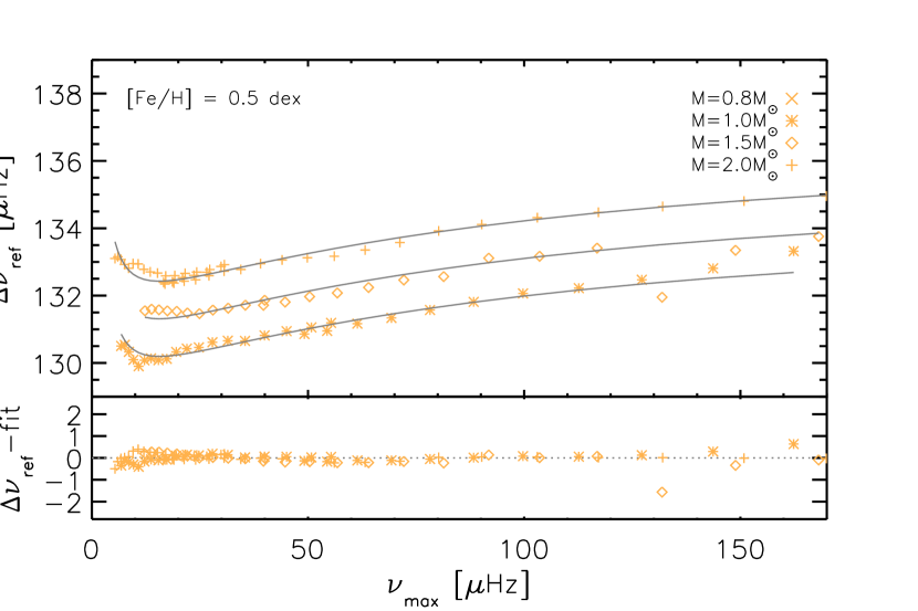
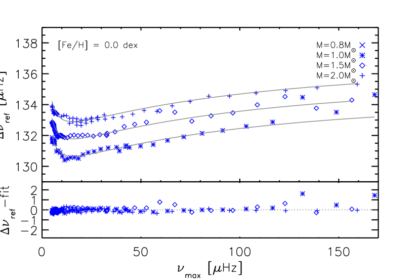
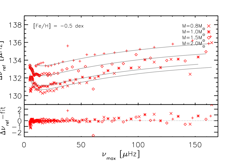
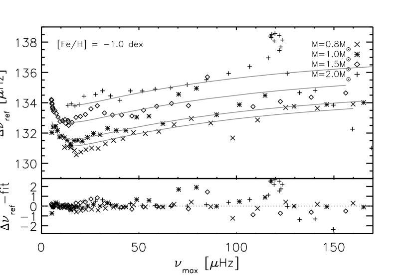
The asteroseismic scaling relations (Ulrich, 1986; Kjeldsen & Bedding, 1995) permit a straightforward inference of fundamental stellar parameters such as the mass and radius of solar-like oscillators (i.e., stars that exhibit stochastic oscillations driven by turbulent convection in their outer layers). These relations require knowledge of the effective temperature and some characteristics of the oscillations that can be derived from timeseries data of either brightness or radial velocity variations. One of these oscillation characteristics is the so-called large frequency separation, , which is defined as the separation between modes of the same degree and consecutive radial orders. The other oscillation parameter is the frequency of maximum oscillation power, . These scaling relations relate and to mean density and surface gravity , and thus mass and radius , in the following way:
| (1) |
| (2) |
where , , , and effective temperature are expressed in solar values. In the initial formulations of these relations the solar quantities are used as reference values, i.e. ref = ⊙ = 135.1 0.1 Hz, (Huber et al., 2011), and = ⊙ = 3050 Hz (Kjeldsen & Bedding, 1995). This approach inherently assumes that the Sun and the star under investigation have similar internal structures. However this assumption is not strictly valid and differences in stellar structure cause systematic errors in the masses and radii (see e.g. Corsaro et al., 2013; Huber et al., 2013; Epstein et al., 2014; Miglio et al., 2012) derived from the scaling relations. Several approaches to correct for the errors have been suggested, including interpolations between precomputed models (Sharma et al., 2016), which requires access to a model grid, as well as analytical formulations (White et al., 2011; Mosser et al., 2013). For a detailed discussion of the available corrections, see Guggenberger et al. (2016, hereinafter Paper I).
In Paper I we used stellar models to derive a reference large frequency separatio that should be used instead of . We modelled the general behaviour of over a wide range of temperatures and metallicities with a damped sinusoid, thereby extending the work of White et al. (2011) to a larger parameter space. The analytical expression presented in Paper I can be applied in a straight-forward manner to compute the optimal reference value from the observables Teff and [Fe/H] and reduces the errors in masses and radii by a factor of two compared to the uncorrected scaling relations. However, on the red-giant branch a dependence on mass remained present in the residuals of (see Fig. 3 of Paper I). The dispersion of the different mass tracks occurs at different temperatures depending on metallicity, ranging from about 4500 K at [Fe/H] = 0.5 to about 5200 K at [Fe/H] = -1.0. In all cases these values correspond to the same evolutionary phase; namely, where the star turns onto the red-giant branch (see e.g. Fig. 2 of Paper I). In the current work we mitigate this mass dependence on the red-giant branch.
2 Methods
2.1 Models and determination
Stellar models were calculated with the the Yale Rotating Stellar Evolution Code (YREC, Demarque et al., 2008). The choice of input physics are as described in paper I with our grid comprising masses of 0.8, 1.0, 1.5 and 2.0 M⊙ and metallicities [Fe/H] = 0.5, 0.0, -0.5 and -1.0 dex. A subset of models along each track were extracted for the analysis such that Hz.
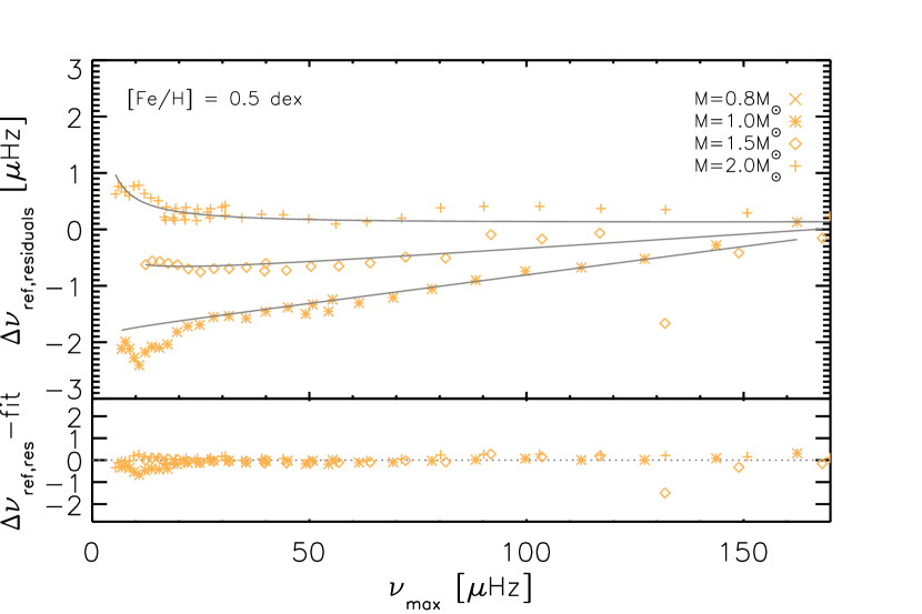
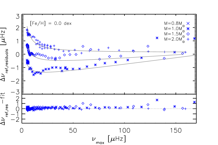
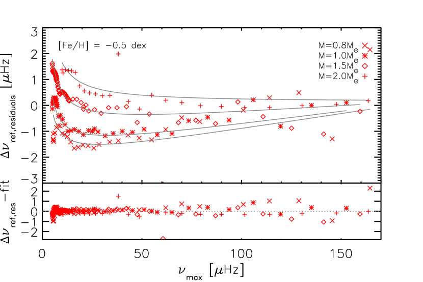
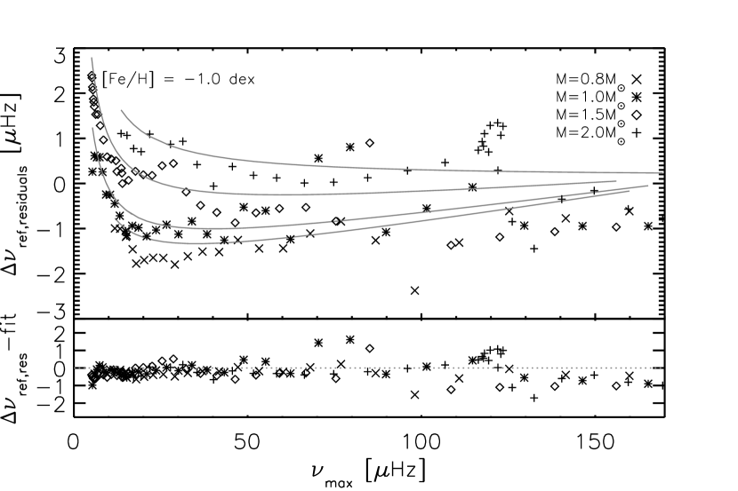
The value of was determined from the models using radial mode frequencies as per Paper I, i.e. using a Gaussian weighted linear fit to the frequencies around the expected , where the full-width at half maximum of the Gaussian is fixed to 5 . From this value of , together with the known model mass and radius, we computed the reference needed to reproduce the model mass and radius from the scaling relation (see Figs 1 and 5). We note that the scatter in increases as a function of decreasing [Fe/H]. The reason for this is currently unknown but this may be due to difficulties in the computation of the mode frequencies. Uncertainties in the frequencies also set the lower limit of the range that we consider.
Finally, we determined an analytical expression that allows the reference value to be calculated straightforwardly for use by the community.
2.2 Symbolic regression
In Paper I we found that the underlying functional form of the reference as a function of resembles a damped sinusoid. The metallicity dependence was then included by investigating how the individual constants of the damped sinusoid behaved when the other parameters of the function were kept fixed. The mass dependence investigated here shows a more complex behaviour. Therefore, we used symbolic regression. Symbolic regression is a type of optimisation that searches mathematical expressions to find a model that best fits the data. Thus rather than searching for the optimal parameters of a pre-defined expression (as is commonly done in regression techniques), the algorithm simultaneously optimizes the functional form and the parameters of the function.
For the work presented here we used the software Eureqa (Schmidt & Lipson, 2009) distributed by Nutonian. This software package uses an evolutionary search to automatically perform symbolic regression.
3 Functions describing the mass dependence
We performed symbolic regression on the values as derived in Paper I as well as on the residuals that remain after applying the fit published in Paper I (). Our investigation revealed that a mass dependency in the correction function is possible if our expression takes the form =(, M, [Fe/H]). We fit the function to stars with 5 Hz 170 Hz as the impact of the mass dependence is significant only in stars with below 170 Hz. For stars with higher we therefore recommend the correction function from Paper I.
The respective functions for ref as well as for the residuals after the correction from Paper I take the form:
| (3) |
| 124.72 | Hz | 1.88 | Hz/M⊙ | |||
| 2.23 | Hz/M⊙ | 0.02 | - | |||
| 17.61 | Hz2 | 5.14 | HzM⊙ | |||
| 0.73 | 10.90 | Hz2 | ||||
| 0.02 | - | 3.69 | Hz | |||
| 0.93 | Hz | 0.01 | M |
| (4) |
with the parameters and units listed in Table 1. We note that these reference functions (Eqs 3 and 4) as well as the reference function in Paper I do not have a clear physical meaning. They do represent however an empirical fit optimised to the data obtained from stellar models that include canonical stellar physics.
Example code for implementing the algorithm is provided in Appendix B.
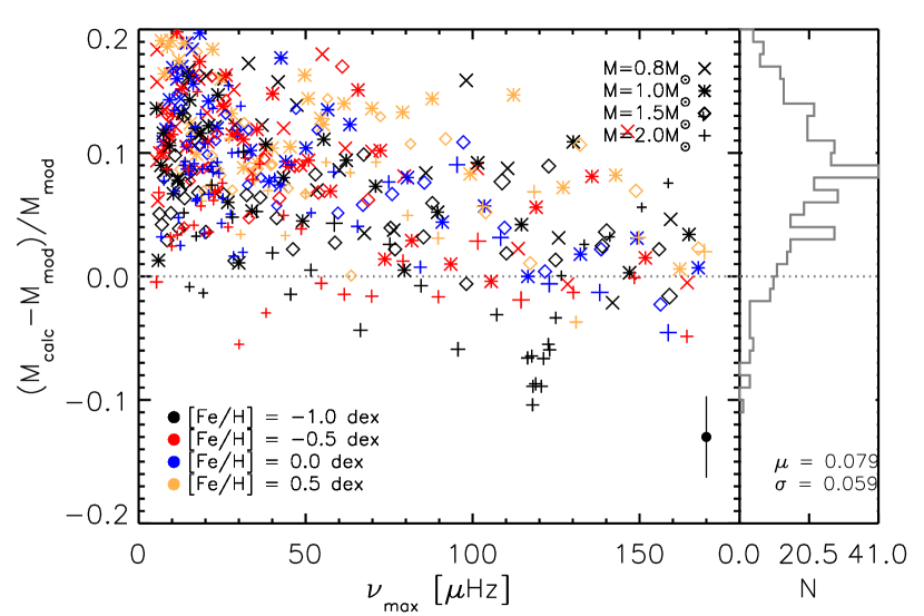
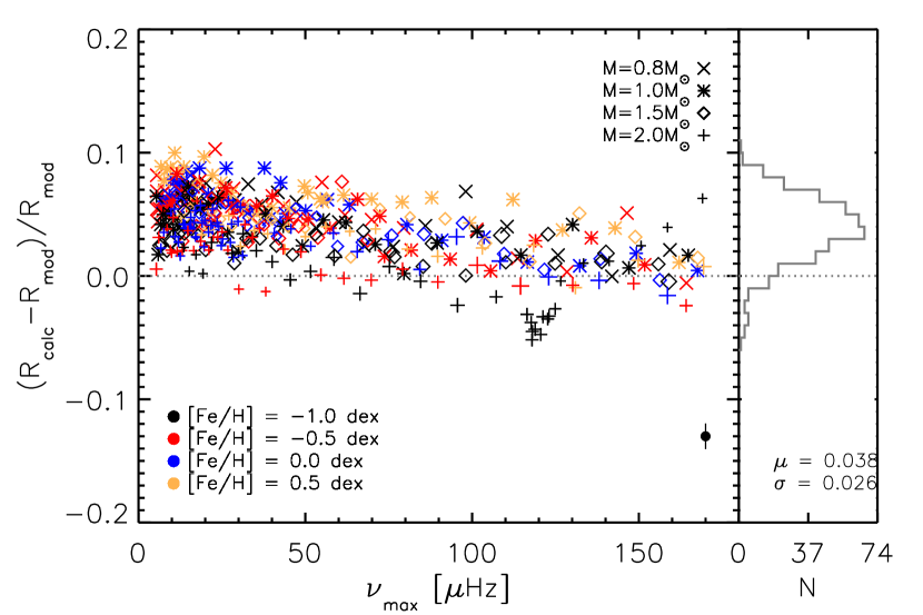
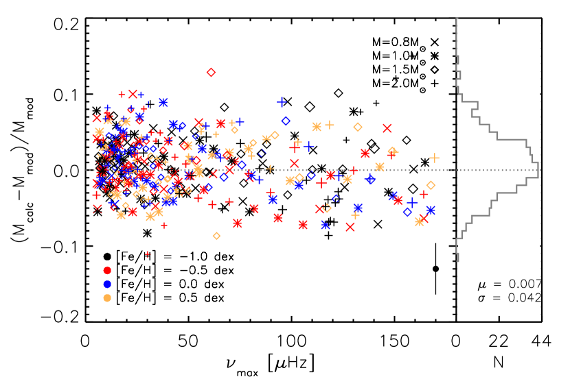
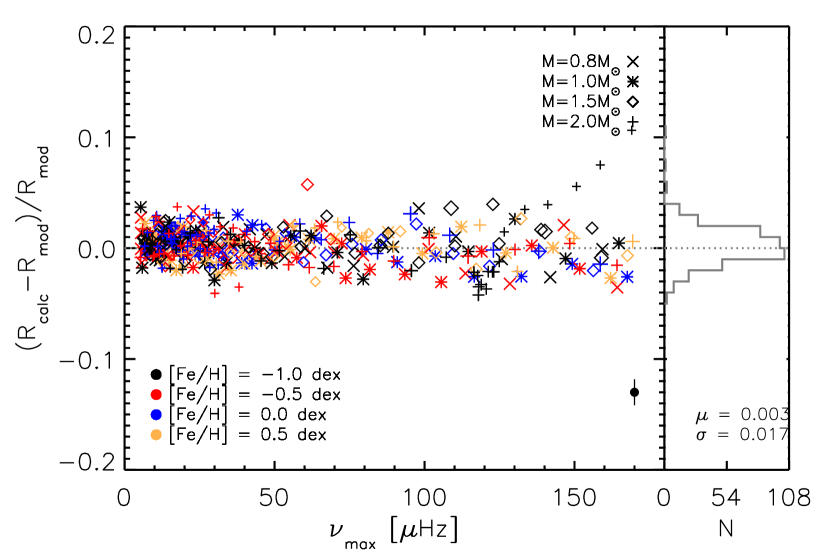
| method | ||||
|---|---|---|---|---|
| solar | 0.075 | 0.050 | 0.037 | 0.024 |
| Eq. 3 | 0.000 | 0.022 | 0.000 | 0.011 |
| solar (perturbed) | 0.079 | 0.059 | 0.038 | 0.026 |
| Eq. 3 (perturbed) | 0.007 | 0.042 | 0.003 | 0.017 |
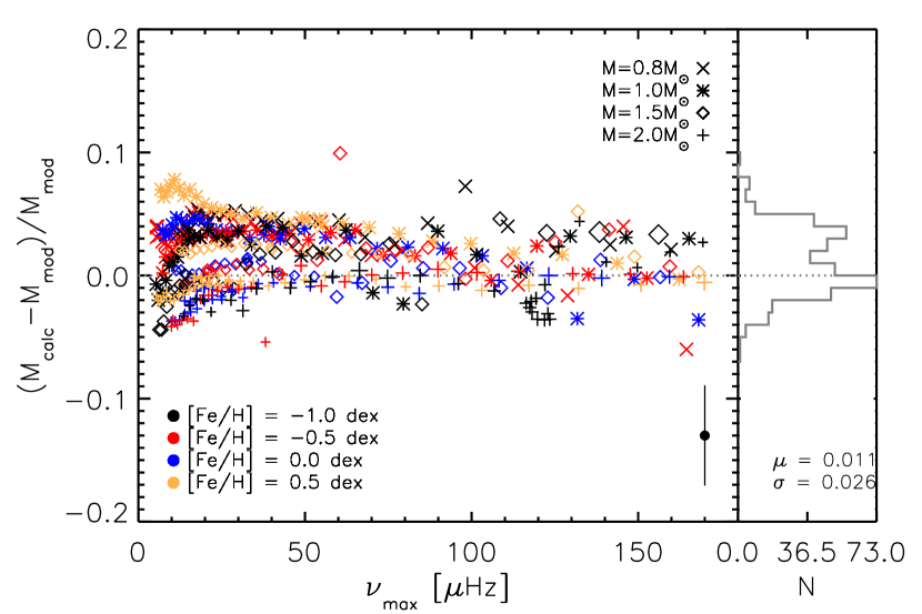
| Paper I | 0.011 | 0.026 | 0.005 | 0.013 |
| Eq. 4 | 0.001 | 0.014 | 0.001 | 0.007 |
| Paper I (perturbed) | 0.015 | 0.049 | 0.006 | 0.020 |
| Eq. 4 (perturbed) | 0.007 | 0.045 | 0.003 | 0.018 |
4 Results
As mass is not known a priori, the procedure we have developed is iterative in nature. An initial estimate of the input mass is determined using the classical (Kjeldsen & Bedding, 1995) scaling relation and the corresponding solar reference values of ref = ⊙ = 135.1 0.1 Hz, (Huber et al., 2011), and = ⊙ = 3050 Hz (Kjeldsen & Bedding, 1995). This mass is then used in Eq. 3 to compute an improved mass. We iterate until the mass remains constant to a level of 0.001 M⊙ which is typically reached in 2-5 iterations.
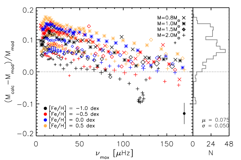
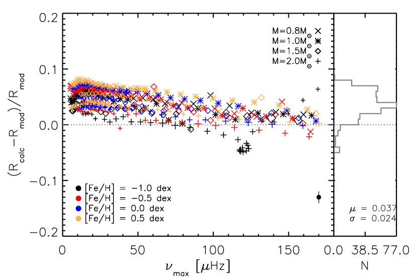
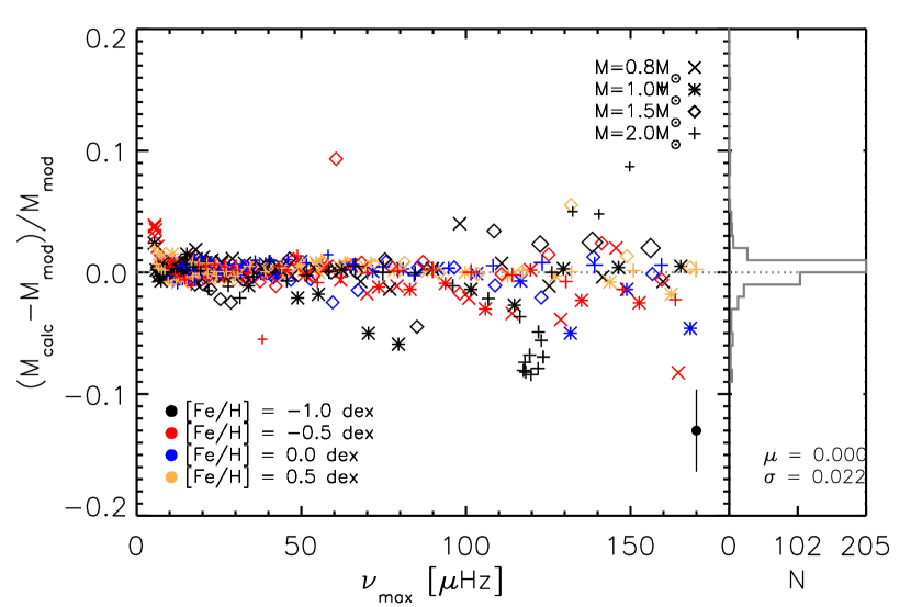
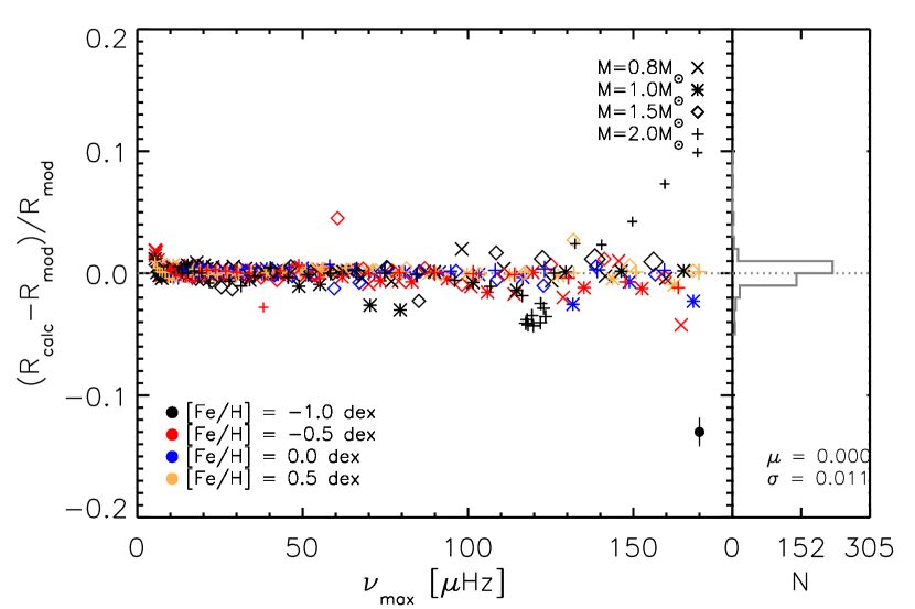
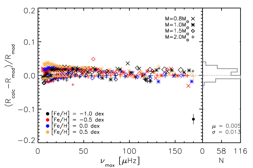
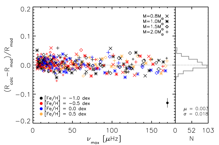
We first demonstrate the efficacy of our fit by predicting the masses and radii for models used in the training grid. We produce 1000 instantiations of each ‘star’ perturbing each observable quantity with Gaussian noise according to a typical measurement uncertainty. We assume uncertainties of 5% on , 0.09 dex in [Fe/H], 85 K in and 0.01 Hz on the frequencies. In this test each faux observable quantity was perturbed around the known values from the stellar model. The relative differences in mass and radius between the values calculated using the scaling relations and the real values are shown in Fig. 2. The mean and standard deviation indicated in each panel of Fig. 2 and in Table 2 indeed show that with the new reference function (Eq. 3) the biases in both mass and radius are mitigated and that the standard deviation is reduced by a factor of 2. Additionally, the dependence on is mitigated by the reference function.
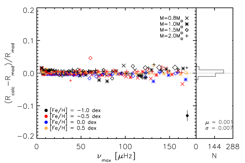
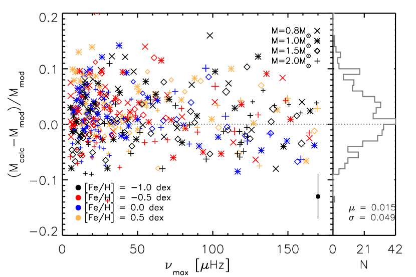
In a second approach we computed an initial mass using the reference function described in Paper I. This mass is then used as an input to the reference function (Eq. 4) to iteratively compute the mass and radius. As per the first function we evaluate the function by perturbing the model data. The results are shown in Figure 6. Again with this function we mitigate the bias of the relative difference in calculated and model values and reduce the standard deviation by roughly a factor of 2. However, this results in standard deviations that are smaller (about ) compared to the results from the first approach.
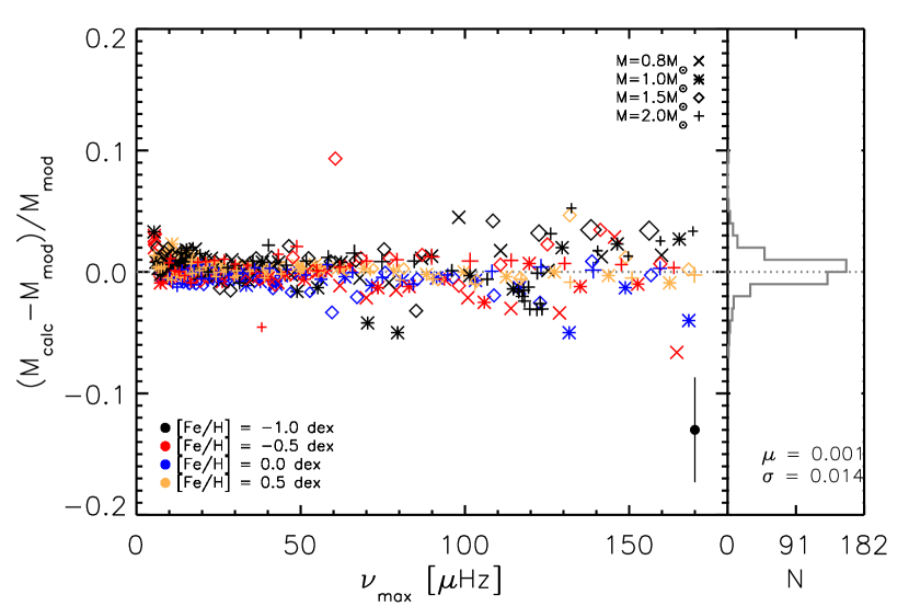
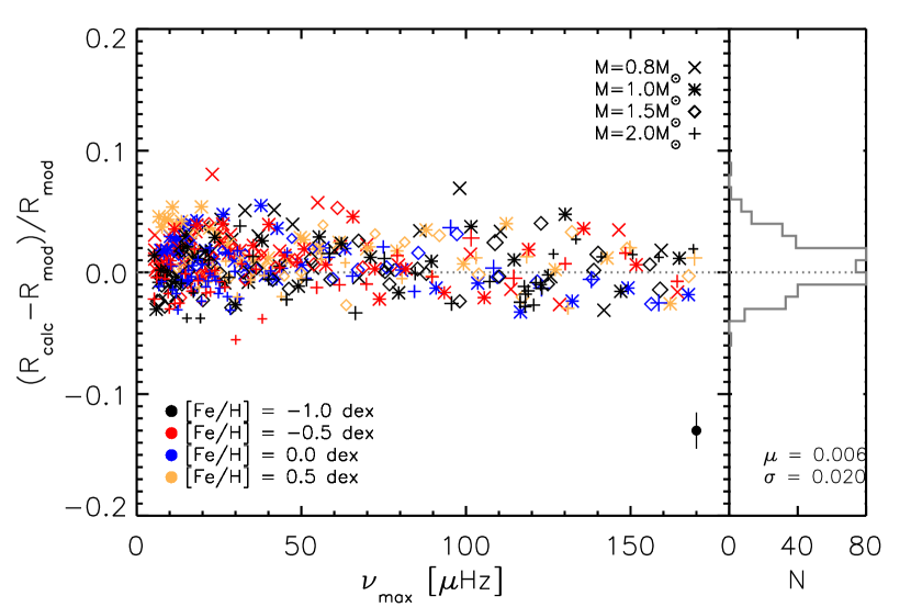
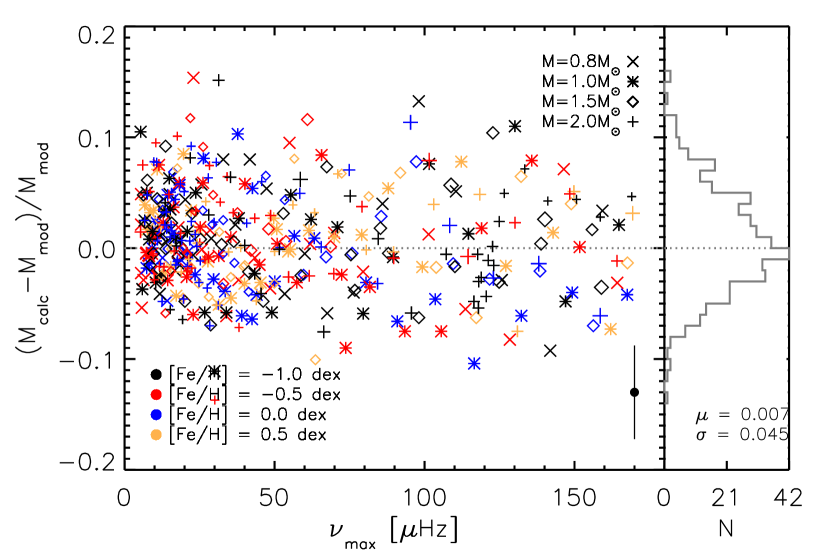
In addition to the test above we also used used perturbed values as our central values. We perturbed the mass, metallicity, effective temperature and individual frequencies in the same manner as before and computed masses and radii using the scaling relations iteratively with the reference functions described in Eqs 3 and 4. The results are shown in Figs 3 and 7. These figures show that the reference functions that we present here indeed remove trends that are present in the mass and radius determinations as a function of and mitigate the biases to a large extent. However, the standard deviations from using either Eq. 3 or Eq. 4 are very similar and significantly larger than in the ‘ideal’ case, showing the impact of uncertainties in the observations.
4.1 Hare-and-Hound Validation
We have thus far demonstrated that the new functions improve mass and radius estimations for the data they fit. In order to prove the general efficacy of our new corrections we appraise the performance of the functions on data to which they have not been exposed. We perform a series of hare-and-hound validations using stellar models calculated with two additional evolution codes. We used GARSTEC (Weiss & Schlattl, 2008) and MESA (Paxton et al., 2011) to compute grids of stellar tracks from which we draw testing data. Over 1000 models from each grid were extracted to serve as hares with the requirements that each selected model falls within the verified mass, metallicity and ranges of the correction functions. The choice of microphysics and modelling assumptions differ between these two codes and they also differ from the code used to calculate the training data in YREC. Thus mass and radius predictions of the hares will indicate the degree of stellar evolution code dependence in our function.
Both the GARSTEC and MESA grid were computed using OPAL opacities (Iglesias & Rogers, 1996) in conjunction with Ferguson et al. (2005) tables at low temperatures. We utilized the updated 2005 tables for the OPAL equation of state (Rogers & Nayfonov, 2002) along with the assumption of an Eddington plane-parallel atmosphere. We have taken the recommended nuclear reaction rates from the NACRE collaboration in combination with those from Caughlan & Fowler (1988). The treatment of convection follows the mixing length theory as described by Kippenhahn et al. (2012) and models were computed with the respective solar calibrated mixing lengths. Radial mode frequencies were calculated with the ADIPLS pulsation package (Christensen-Dalsgaard, 2008) for the GARSTEC models and with the GYRE pulsation package (Townsend & Teitler, 2013) for the MESA models. The large frequency separation determined using a weighted median around the scaled as per Bellinger et al. (2016).
The grids differ in that the GARSTEC models assume Asplund et al. (2009) solar abundances and were computed without overshoot or atomic diffusion. In contrast, the MESA grid employs the Grevesse & Sauval (1998) solar composition. For the MESA models we use a step overshooting prescription at all convective boundaries with an efficiency of 0.08 pressure scale heights. Additionally, atomic diffusion as per Thoul et al. (1994) is included in tracks up to and its efficiency smoothly reduced thereafter.
The hares comprise 1095 models from the GARSTEC grid with 15 models extracted along the RGB of 73 different evolutionary tracks. We also include 1492 models from the MESA grid having selected four models from 373 individual tracks.
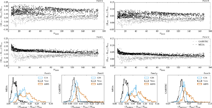
The results of the hare-and-hound validation for the extracted models are presented in the seven panels in Fig. 4. Figures 4a and 4b show the relative errors in the predictions for mass and radii using the correction outlined in Paper I. The corresponding relative differences after applying Eq. 3 are shown in Figs 4c and 4d. In Figures 4e-h we plot the error distributions for each code and parameter. We include in these panels the predictions from the Paper I correction (G16), Eq. 3 (New) as well as the classic Kjeldsen & Bedding (1995) scaling relation (KB95).
Our results indicate that there is a systematic offset between MESA models and those from the other two codes. The offset can be explained by a different temperature scale in the RGB models that is caused by a larger mixing-length parameter used in the MESA models that originates from a solar calibration that includes elemental diffusion. The corresponding change to and by reducing the MESA models by 15 K is sufficient to centre its error distributions around the zero point (such that they lay on top of the GARSTEC points). We note also that the GARSTEC models diverge from the YREC models as a function of evolution as seen by the trend in which is to be expected when comparing models with and without atomic diffusion (see e.g. Michaud et al. 2004).
5 Discussion and Conclusions
We have found two reference functions for the scaling relation of the large frequency separation that mitigate the mass dependence. We have shown that these results are valid for stellar models in the range 5 Hz 170 Hz and improve the mass and radius determinations by 10% and 5% respectively (compared to the solar reference). This is true in the limit of ideal data obtained from canonical stellar models and no surface effects in which these functions provide a better underlying model to use when applying the scaling relation. Therefore, this method can be assumed to be valid for stars that do not show any extreme physics (e.g. large magnetic fields).
If we assume observational uncertainties on , and [Fe/H] the devised reference functions continue to improve the accuracy of the masses and radii as in the ideal case. However, the precision depends on the observational uncertainties. In theory it is better to fit the residuals (hence the equation from Paper I combined with Eq. 4). However, in practice observational uncertainties dominate and there is minor difference between using Eq. 3 and Eq. 4.
We have also tested the reference functions on a large number of models computed with MESA (Paxton et al., 2011) and GARSTEC (Weiss & Schlattl, 2008). From these tests it is clear that the underlying form is correct. However, we found that a slight offset in temperature will propagate to differences in that in turn influence the accuracy of the derived masses and radii. Optimising the coefficients of the functions described in Eqs 3 and 4 would mitigate this offset.
Acknowledgements
The research leading to the presented results has received funding from the European Research Council under the European Community’s Seventh Framework Programme (FP7/2007-2013) / ERC grant agreement no 338251 (StellarAges). S.B. acknowledges partial support of NASA grant NNX16AI09G and NSF grant AST-1514676.
References
- Asplund et al. (2009) Asplund M., Grevesse N., Sauval A. J., Scott P., 2009, ARA&A, 47, 481
- Bellinger et al. (2016) Bellinger E. P., Angelou G. C., Hekker S., Basu S., Ball W. H., Guggenberger E., 2016, ApJ, 830, 31
- Caughlan & Fowler (1988) Caughlan G. R., Fowler W. A., 1988, Atomic Data and Nuclear Data Tables, 40, 283
- Christensen-Dalsgaard (2008) Christensen-Dalsgaard J., 2008, Ap&SS, 316, 13
- Corsaro et al. (2013) Corsaro E., Fröhlich H.-E., Bonanno A., Huber D., Bedding T. R., Benomar O., De Ridder J., Stello D., 2013, MNRAS, 430, 2313
- Demarque et al. (2008) Demarque P., Guenther D. B., Li L. H., Mazumdar A., Straka C. W., 2008, Ap&SS, 316, 31
- Epstein et al. (2014) Epstein C. R., et al., 2014, ApJ, 785, L28
- Ferguson et al. (2005) Ferguson J. W., Alexander D. R., Allard F., Barman T., Bodnarik J. G., Hauschildt P. H., Heffner-Wong A., Tamanai A., 2005, ApJ, 623, 585
- Grevesse & Sauval (1998) Grevesse N., Sauval A. J., 1998, Space Sci. Rev., 85, 161
- Guggenberger et al. (2016) Guggenberger E., Hekker S., Basu S., Bellinger E., 2016, MNRAS, 460, 4277
- Huber et al. (2011) Huber D., et al., 2011, ApJ, 743, 143
- Huber et al. (2013) Huber D., et al., 2013, Science, 342, 331
- Iglesias & Rogers (1996) Iglesias C. A., Rogers F. J., 1996, ApJ, 464, 943
- Kippenhahn et al. (2012) Kippenhahn R., Weigert A., Weiss A., 2012, Stellar Structure and Evolution. Springer-Verlag Berlin Heidelberg, doi:10.1007/978-3-642-30304-3
- Kjeldsen & Bedding (1995) Kjeldsen H., Bedding T. R., 1995, A&A, 293, 87
- Michaud et al. (2004) Michaud G., Richard O., Richer J., VandenBerg D. A., 2004, ApJ, 606, 452
- Miglio et al. (2012) Miglio A., et al., 2012, MNRAS, 419, 2077
- Mosser et al. (2013) Mosser B., et al., 2013, A&A, 550, A126
- Paxton et al. (2011) Paxton B., Bildsten L., Dotter A., Herwig F., Lesaffre P., Timmes F., 2011, ApJS, 192, 3
- Rogers & Nayfonov (2002) Rogers F. J., Nayfonov A., 2002, ApJ, 576, 1064
- Schmidt & Lipson (2009) Schmidt M., Lipson H., 2009, Science, 324, 81
- Sharma et al. (2016) Sharma S., Stello D., Bland-Hawthorn J., Huber D., Bedding T. R., 2016, preprint, (arXiv:1603.05661)
- Thoul et al. (1994) Thoul A. A., Bahcall J. N., Loeb A., 1994, ApJ, 421, 828
- Townsend & Teitler (2013) Townsend R. H. D., Teitler S. A., 2013, MNRAS, 435, 3406
- Ulrich (1986) Ulrich R. K., 1986, ApJ, 306, L37
- Viani et al. (2017) Viani L. S., Basu S., Chaplin W. J., Davies G. R., Elsworth Y., 2017, preprint, (arXiv:1705.03472)
- Weiss & Schlattl (2008) Weiss A., Schlattl H., 2008, Ap&SS, 316, 99
- White et al. (2011) White T. R., Bedding T. R., Stello D., Christensen-Dalsgaard J., Huber D., Kjeldsen H., 2011, ApJ, 743, 161
Appendix A Fits and Residuals
Here we present the figures obtained using first the reference function presented in Paper I and subsequently the fits as described in Eq. 4.
Appendix B Example Code
Here we provide some example code in both Python and IDL of the iterative process to determine masses and radii with the reference function for presented in this work.