Uncertainty in Economic Growth and Inequality

Abstract

A step to consilience, starting with a deconstruction of the causality of uncertainty that is embedded in the fundamentals of growth and inequality, following a construction of aggregation laws that disclose the invariance principle across heterogeneous individuals, ending with a reconstruction of metric models that yields deeper structural connections via U.S. GDP and income data.

1   Motivation

With a simple belief about facts that must be, Laozi in the 6th BCE deems the phenomena that are wholly in harmony behaving in a completely natural and uncontrived way. He says, “Nature does nothing, but everything is done.” A similar economic ideology, laissez faire used by the physiocrats in the 17th century or later invisible hand used by Adam Smith on income distribution and production, has been deeply rooted in the core of modern economic analysis. In this perspective, individuals optimize decisions, markets rationalize deals, different forces stabilize interferences, and so equilibria are established, as an outcome of these self-organized dynamics, which in principle should lead us to a well-acceptable status.

However when one turns to another perspective viewing these economic elements as an integrated, evolving and continuous entity, one may lose oneself in a chaotic, intricate, and unordered retrospective of economic history. Economic system is consistently vibrating. Individuals are incapable of seizing their own fates, markets tend to generate various bubbles, political forces weave a gravity field making things fallen. The commonly accepted equilibria seem to be in an unreachable state. The dynamical process, instead of driving us to a utopia, constructs a predicament of mankind concealing the problems origins. Joseph Schumpeter in [9] writes the following words, “The essential point to grasp is that in dealing with capitalism we are dealing an evolutionary process. It may seem strange that anyone can fail to see so obvious a fact which moreover was long ago emphasized by Karl Marx. […] Capitalism, then, is by nature a form or method of economic change and not only never is but never can be stationary.”

One ostensible reason of this inconsistency is that models and their assumptions are merely abstractions or oversimplifications of the reality, thus it would be natural that they fail to consider some of these phenomena. It would be even more natural to attribute these unexplained imperfections to a category caused by uncertainty and then let it explain them, since by definition uncertainty is uncertain and is hard to be merged into a system that is certain. But what if there is no inconsistency? What if everything is in order and one unpleasant outcome in an economy is just a consequence of a sequence of pleasant decisions well-accepted amongst individuals? What if in this sequence uncertainty will certainly bring in the denouement?

A crux is the role of uncertainty. Current treatment on uncertainty is to separate it from the fundamentals of economic theory while expecting it to conciliate the contradictory theories about how to interpret the existing phenomena. The gap between two perspectives, as long as it does not affect the self-consistencies in either domain, is considered to be harmless. Nevertheless, there may exist another perspective: all things return to uncertainty. It could be the uncertainty that manipulates the economy, that shapes the social order, that generates and wipes out our expectations. In such a case, uncertainty is no longer the bridge over the gap, it eliminates the gap. This faith is simple: diverse individual decisions reflected by their own beliefs about the laws of this uncertain world, after rationalization, integration and evolution, converge to a field that is characterized by a certain law, an invariant of the individuals’. Uncertainty, therefore, is certain.

Return to the controversial fundamentals. Two basic opposites co-exist along the economic history: growth and inequality. About their causal relationship, [7] asks the following question “Does inequality in the distribution of income increase or decrease in the course of a country’s economic growth?” He did not answer this dualism question in [7], nor elsewhere to my best knowledge. The dilemma is that the obvious answer seems to contradict the righteousness in theory while in the rigid dichotomy the alternative answer is too ambiguous to be believed as a law. In the history of economy, when new products are introduced there is an intense amount of research and development which leads to dramatic improvements in quality and reductions in cost. This leads to a period of rapid economic growth. However, the owners of these new products, at the time of their occurrences, stand in sharp contrast to the great mass of their contemporaries. Every advance first comes into being innovation developed by one or few persons, only to become, after a time, the indispensable necessity taken for granted by the majority. Equality does not seem to exist at the very beginning of the growth. The opportunities of quality improvement and cost reduction are gradually exhausted, then the products are in widespread use and the trend turns into alleviating such an inequality but also growth. Stimulus in production caused by the inequality is considered as an abstract source, full of uncertainties. Thus entanglement of growth and inequality, like other controversial fundamentals, masks the causality behind complex stochastic patterns.

Economic growth and inequality, from the most causal matters of divergences in incomes and wages to the profoundest concentration of capital, is from my perspective a man-made configuration. Growth is a human right of surviving and propagating while equality is a human desire rooting deeply in the conscious and belief. How would the invisible hands dispose the relationship of these two basic elements? Enlightened by theories and methodology in [10], this paper considers uncertainty as a composition of more elementary stochastic components available amongst individuals then formulate concrete dynamics using laws extracted from individuals. Deconstruction of uncertainty makes it feasible to epistemologically discuss previous questions. Abstraction of inequality as a limit aggregation law of economic growth concretizes its representation. All these are done with the preservation of two basic elements, growth and equality, over individuals. Uncertainty of growth entails the laws by which inequality is invariantly revealed. The latter is so determined by its intrinsic equality conditions that there is few choice left to an attempt of wiping it out, even at the fundamental level.

2   Guide

Section 3 is a preliminary where the connection with mainstream growth model is established but the substance emphasizes the use of new assumptions. Section 4 extends the set of new assumptions to a more general setting in order to incorporate with uncertainty. Equilibrium is shown to be in existence and its law is unique for each individual. Individuals are endowed with stationary probabilistic laws for the equilibrium growth. Section 5 shifts the attention to aggregates. Infinite divisible law is introduced. Individual’s law becomes aggregatable. Non-stationary aggregates are distinguished from stationary aggregates. The latter ones follow the same law as individuals’ while the former ones need some additional characterization. Section 6 exploits structural relationship between individual and aggregate laws. Aggregation of laws is represented by summing and scaling of structural parameters. These parameters reveal possible latent movements. Some of them conflict with superficial facts. Section 7 uses data to illustrate some theoretical arguments. Some forward-looking thoughts are refined in Section 8. Proofs, if necessary, are given in the appendix. Some proofs are chosen to be heuristic so that they are accessible to readers with general mathematical background. Each main section is followed by general remarks summarizing its main theme.

3   A non-abstract model

It is sometimes said that societies have to choose between greater equality and economic growth. This section shows an ideal growth model that can achieve the equal status regardless of initial heterogeneities amongst different individuals. It reveals that growth does not necessarily have negative correlation with equality. Once we separate the causality between growth and equality, we examine different objectives of growth and equality and see how these differences consequently consolidate and become coherent in the equilibrium. All these arguments rely on three assumptions.

3.1 Scarcity, growth, and equality

Let $X_{t}(\omega^{i})$ denote an economic variable of individual $i$ at time $t$ with an initial state $X_{0}^{i}=\omega^{i}$, such as a capital intensity. Suppose $\omega^{i}\in\Omega$ and $X_{t}(\omega^{i})\in\Omega$ for any $t$ and $i$. For the simplest case, we assume that the set $\Omega$ is on a closed and bounded interval. When there is no necessity for emphasizing a specific individual, sometime $X_{t}(\omega)$ may refer to any individual.

Assumption 1.

The set $\Omega$ is on a closed and bounded interval in $\mathbb{R}$. Without loss of generality, we assume $\Omega=[0,1]$.

This assumption reflects that each individual faces the scarcity of economic resources. The assumption applies to both initial endowments $\omega^{i}$ and future states $\{X_{t}(\omega^{i})\}_{t>0}$ of this individual. It eliminates the possibility of unbounded growth for any individual $i$.

Assumption 2.

Assume the growth function $f$ of this economic variable as a real-valued monotone non-decreasing function $f(\cdot):\Omega\rightarrow\Omega$ where $X_{t}(\omega^{i})=f^{(t)}(\omega^{i})=f(f^{(t-1)}(\omega^{i}))$ for $t=1,2,\dots$.

This assumption gives a non-decreasing growth function. With Assumption 1, these two assumptions induce that any individual in this economy will ultimately reach his or her equilibrium status. Because $f(\cdot)$ is a monotone function on $[0,1]$, any sequence of $f^{(t)}(\cdot)$ converges as $t\rightarrow\infty$. Otherwise, either there exists a divergent sequence that will violate the condition of monotonicity or the sequence $f^{(t)}$ will go beyond the bounded interval $[0,1]$.

Consider two households with initial endowment $0$ and $1$ respectively. At time $t$, their economic variables become $X_{t}(0)=f^{(t)}(0)$ and $X_{t}(1)=f^{(t)}(1)$. The convergent property of $f$ entails $X_{t}(0)\uparrow X^{*}(0)$ and $X_{t}(1)\downarrow X^{*}(1)$ where $X^{*}(0)$ and $X^{*}(1)$ are the convergent limits and $X^{*}(0)\leq X^{*}(1)$.

Assumption 3.

Two limits $X^{*}(0)$ and $X^{*}(1)$ of the convergent sequences $X_{t}(0)$ and $X_{t}(1)$ are equivalent.

This assumption implies an ideology of equality, as the individual with the smallest initial endowment is assumed to be able to achieve the same equilibrium state as those with the biggest endowment $X^{*}(0)=X^{*}(1)$. Because everyone in this economy has a convergent $X^{*}(\omega)$ and because any $X^{*}(\omega)$ should be not smaller than $X^{*}(0)$ and not larger than $X^{*}(1)$, we have $X^{*}(\omega)=X^{*}(0)=X^{*}(1)$. The fact is that for any individual with any initial state $\omega\in[0,1]$, when $t\rightarrow\infty$ such an individual will attain the same limit $X^{*}(\omega)$ as the others. Thus $X^{*}(0)$ is the unique fixed point of the limit of $\{X_{t}(\omega)\}_{t}$ for any $\omega\in\Omega$. This result is summarized in the following theorem.

Theorem 1.

Given Assumption 1 to 3, the economy reach an equal status, namely any $X_{t}(\omega^{i})$ converges to the same $X^{*}$ .

These three assumptions play different roles. Assumption 1 allows for heterogenous initial states for all individuals and allows us to identify their wealth levels especially those at the extremes. Assumption 2 imposes the same growth function $f(\cdot)$ to all individuals with different endowments. The monotone non-decreasing $f(\cdot)$ implies that growth happens for all individuals. Assumption 3 is analogous to the statement “all men are created equal”, because it assumes that the poor and the rich will come to the same state. The inequality exists at the very beginning due to the heterogenous initial endowments, but with the same growth function, eventually the inequality vanishes in this economy.

3.2 A Growth Model for $N$ Individuals

Although it looks simple, the previous specification can illustrate some essences in framework of the classic Solow growth model. In Solow’s framework, the economic variable $X_{t}$ refers to capital per labor such that $X_{t}=K_{t}/L_{t}$. Provided that the production function $f_{P}(K_{t},L_{t})$ has constant returns to scale, one can set the production per labor to $f_{P}(X_{t},1)$. The growth function refers to the fundamental equation of the Solow model

$$X_{t+1}=f(X_{t})=\beta_{1}f_{P}(X_{t},1)-(\beta_{2}-1)X_{t}$$

where $\beta_{1}$ is the saving rate and $\beta_{2}$ is the effective depreciation rate of capital per labor.

Given an arbitrary number of individuals $N$ in this economy, these individuals provide labor and rent capital in a competitive labor and capital market, they have access to the same neoclassical technology, and produce a homogeneous output. For a monotone $f(\cdot)$ and $X_{t}=K_{t}/L_{t}$ in $\Omega$, there exists one $X^{*}$. If the poorest and the richest can reach the same level of production in the long run, then Theorem 1 assures a unique fixed point for all initial endowments $\omega^{i}\in\Omega$. Therefore for any individual, $f(X_{t})\rightarrow X^{*}$ as $t\rightarrow\infty$. In the equilibrium, the production function becomes

$$f(X^{*})=\beta_{1}A_{S}^{*}+\left(\beta_{1}B_{S}^{*}+1-\beta_{2}\right)X^{*}$$

where $B_{S}^{*}$ and $A_{S}^{*}$ are equilibrium coefficients satisfying the fixed point result $f(X^{*})=X^{*}$ which coincides with the result in the classic Solow model.The value $X^{*}$ is independent of the initial endowment $\omega$. One can conclude that for any initial state $\omega\in[0,1]$, the equilibrium $X^{*}$ makes all individuals access to the same production type as they use exactly the same capital-labor ratio.

Moreover, a linear aggregation is simplified as a summation of $N$ identical $X^{*}$s when $t\rightarrow\infty$. The growth function

$$f\left(N\times X^{*}\right)=N\times X^{*}.$$

induces the stability of the structure. It refers to the fact that the aggregate growth acts as if it was a non aggregated function of individuals. The aggregation process does not distort the individual growth function in the limit.

3.3 Remarks

Assumption 1 to 3 restrict our attention to one simple model with $N$-individuals. In this model, individuals share the same growth function but at the end they reach the same status. This model implies that individual deterministic growth itself may not generate inequality, on the contrary, it may alleviate inequality. In this $N$-individuals economy, when an equilibrium capital-labor ratio exists and its existence is independent of the initial state $\omega$ for any individual, then eventually the productions of individuals converge to the same level. This economy is homogenized as the inequality together with heterogeneous growth features vanish amongst the individuals. Another implication is that the linear aggregation may not distort the growth if the deterministic economy stays in its equilibrium.

In reality, economic growth often accompanies with greater inequality. Inequality may be enlarged by some relevant factors driven by the growth as well as the initial heterogenous states. Given their unrealistic implications, Assumption 1 to 3 will not be used afterwards. However, the enlightenment of these assumptions is that without uncertainty some specification can drive a growing economy with heterogeneous individuals to an equality status. With this enlightenment in mind, we introduce uncertainty to the economy in order to accommodate more general and realistic dynamics. The new model accommodates the criteria of scarcity, growth and equality in a wider sense.

4   An Abstract Model

There are several ways of introducing uncertainty to growth models. One may think of multiple equilibria or unstable dynamics or statistical errors. These methods usually need some rigid conditions for the aggregation and can only compile limited types of uncertainty. Instead of adding uncertain features to the aggregates, we search for probabilistic laws that relate to both individuals and aggregates. Individuals are governed by these laws, meanwhile a similar law is automatically attached to the aggregates.

Such probabilistic laws are formed in an equilibrium economy. This section provides the result of this equilibrium economy. Three new assumptions are proposed. The new assumptions are comparable with the previous deterministic ones. The result says that the probabilistic law of any individual growth is a stationary distribution that is independent identical across all individuals in this equilibrium economy.

4.1 Abstract Assumptions

We consider an abstract dynamical economy that is a space of $N$-individuals

$$\left((\Omega,\mathcal{B},(\mathcal{B}_{t}),\mathbb{P}),\mathcal{A},f\right)^{\otimes N}.$$

We allow $N$ to grow so that we can represent a large economy with possibly arbitrary number of individuals. The space $(\Omega,\mathcal{B},(\mathcal{B}_{t}),\mathbb{P})^{\otimes N}$ is an $N$-folds of a filtered probability space including a state space $\Omega$, a filtration $\mathcal{B}_{1}\subseteq\mathcal{B}_{2}\subseteq\cdots$ such that $\lim_{t\rightarrow\infty}\mathcal{B}_{t}\rightarrow\mathcal{B}$, and an unknown probability law $\mathbb{P}$ for each individual. The set $\mathcal{A}^{\otimes N}$ is an $N$-folds arbitrary index set for an $N$-folds growth function $f^{\otimes N}$. Each individual $i$ has the growth function $f:\Omega\rightarrow\Omega$ indexed by $a_{t}\in\mathcal{A}$ such as $f^{(a_{t})}(\omega^{i})$. In this economy, a sequence of measurements of dynamical variables (vectors) on $\Omega$ are collected over time. For example the first measurement of the variable $X$ of individual $i$ is denoted as $X_{1}(\omega^{i})=f^{(a_{1})}(\omega^{i})$. If an argument is true for any $i$, there is no necessity of emphasizing $i$. In this case, we can drop $i$ and express $X_{t}(\omega)$ for a variable of an arbitrary individual at time $t$.

Assumption 4.

(Abstract scarcity) In the economy $\left((\Omega,\mathcal{B},(\mathcal{B}_{t}),\mathbb{P}),\mathcal{A},f\right)^{\otimes N}$, each individual faces an identical set $\Omega$ of potential states. Given a total ordered set $\mathcal{P}$ such that $\Omega\subset\mathcal{P}$. we assume that $\mathcal{P}$ is a complete lattice so that the set $\Omega$ has an infimum $\underline{\Omega}\subset\mathcal{P}$ and a supremum $\overline{\Omega}\subset\mathcal{P}$.

Assumption 4 generalizes Assumption 1. Since the number of individuals is allowed to grow to infinity and we assume that each individual faces the same set of potential states, the topological structure of $\Omega$ for all possible states in this economy needs to be extended. This previous setting $\Omega=[0,1]$ is a special case of the total order set with a complete lattice in $\mathbb{R}$. The total ordered structure $(\mathcal{P},\leq)$ assures that the individual is able to compare and rank any two elements from $\Omega\subset\mathcal{P}$. The complete lattice structure states that the individual face scarcity in a wider sense. In the deterministic scarcity $\omega\in[0,1]$, $\omega$ has to be a scalar value while $\omega\in\Omega$ in Assumption 4 is endowed with a general set theoretic structure. This assumption implies that an unlimited want of economic elements in $\Omega$ is impossible.

Assumption 5.

(Individual stochastic growth) The index sequence $\mathbf{a}:=\{a_{t}\}$ is a sequence of i.i.d. random variables $a_{t}$ taking values in the set $\mathcal{A}$. For any sequence $\mathbf{a}\in\mathcal{A}$, there exists a subsequence $\{a_{t}^{{}^{\prime}}\}$ such that function $f^{(a_{t}^{{}^{\prime}})}(\cdot):\Omega\rightarrow\Omega$ is a monotone non-decreasing. For any $x$ and $y$ in $\Omega$, the set $\{\mathbf{a}:f^{(\mathbf{a})}(x)\leq y\}$ is measurable in $(\Omega,\mathcal{B},(\mathcal{B}_{t}),\mathbb{P})$.

Assumption 5 is a stochastic counterpart of Assumption 2. In Assumption 2, every $\{f^{(a)}(\cdot)\}_{a\in\mathcal{A}}$ needs to be monotone while Assumption 5 only requires that every $\{f^{(a)}(\cdot)\}_{a\in\mathcal{A}}$ has at least one monotone subsequence $\{f^{(a_{t}^{{}^{\prime}})}(\cdot)\}_{t\in\mathbb{N}}$ and the index set $\{a_{t}^{{}^{\prime}}\}_{t\in\mathbb{N}}$ of this subsequence is a random variable that is measurable.

The consequence of Assumption 1 and 2 is that any $X_{t}(\omega)=f^{(t)}(\omega)$ will converge to a limit as $t\rightarrow\infty$ regardless of its initial endowment. This consequence does not hold in the stochastic setting. However, Assumption 4 and 5 can induce a similar proposition in a wider-sense. With Assumption 4 and 5, we have the Markov property in Lemma 1 and convergences of the probabilities for individuals with infimum or supremum initial endowments in Lemma 2. Proposition 1 states that the convergent probabilities are stationary for these Markov processes.

Lemma 1.

Given Assumption 4 and 5, $X_{t}(\omega)$ is a Markov process.

Lemma 2.

For any $\{f^{(a)}(\cdot)\}_{a\in\mathcal{A}}$, select a sequence $\mathbf{a}=\{a_{t}\}$ and denote $X_{t}(\cdot)=f^{(a_{t})}(\cdot)$. If Assumption 4 and 5 are true, any $\Pr(X_{t}(\underline{\Omega})\leq y)$ is non-increasing in $t$ and $\Pr(X_{t}(\overline{\Omega})\leq y)$ is non-decreasing in $t$. Hence, $\Pr(X_{t}(\underline{\Omega})\leq y)$ and $\Pr(X_{t}(\overline{\Omega})\leq y)$ are convergent for each $y$.

Proposition 1.

If Assumption 4 and 5 hold and $\mathbb{P}\left(X^{*}(\underline{\Omega})\in\mathcal{X}\right)=\lim_{t\rightarrow\infty}\Pr(X_{t}(\underline{\Omega})\in\mathcal{X})$ and $\mathbb{P}\left(X^{*}(\overline{\Omega})\in\mathcal{X}\right)=\lim_{t\rightarrow\infty}\Pr(X_{t}(\overline{\Omega})\in\mathcal{X})$ for some subset $\mathcal{X}\subset\Omega$, then $\mathbb{P}\left(X^{*}(\underline{\Omega})\in\mathcal{X}\right)$ and $\mathbb{P}\left(X^{*}(\overline{\Omega})\in\mathcal{X}\right)$ are stationary.

Proposition 1 is analogous to the existence of fixed points in the deterministic case. Stationarity is a way of characterizing invariant property in stochastic models. The invariance property of these probability measure implies a Markov equilibrium. A Markov equilibrium is the stochastic analogue of a steady state in the deterministic model. The individual growth process is Markovian and its convergent distribution is stationary when $t\rightarrow\infty$.

To obtain the uniqueness result of the stationary distributions of all individuals, we need an assumption that is similar to the equality condition $X^{*}(1)=X^{*}(0)$ in Assumption 3. Because all convergences are for probability measures, the equality concept should also be adapted to a probabilistic setting. The following assumption supposes that the poor and the rich may be allocated to any possible states in the future. If these re-allocations can happen in probability, it automatically implies the others in the economy should face similar possibilities too. Since everyone has a stochastic monotone growth function and everyone can probably has his or her status changed to any other states, then in the long run, everyone’s growth transition probability may converge to the same stationary distribution as that of the initially rich or poor person. This implication is concretized in Theorem 2 given an assumption about the extreme initial states are not absorbing states.

Assumption 6.

(Equality in probability) For any subset $\mathcal{X}\subset\Omega$, there exists some time $\tau$ such that

$$\Pr\left(X_{t}(\underline{\Omega})\in\mathcal{X}\right)>0,\;\mbox{and},\;\Pr\left(X_{t}(\overline{\Omega})\in\Omega\backslash\mathcal{X}\right)>0$$

when $t\geq\tau$.

Theorem 2.

Given Assumption 4 to 6, then there is a unique stationary distribution such that

$$\mathbb{P}\left(X^{*}(\underline{\Omega})\in\mathcal{X}\right)=\mathbb{P}\left(X^{*}(\overline{\Omega})\in\mathcal{X}\right)=\mathbb{P}\left(X^{*}(\omega)\in\mathcal{X}\right)$$

where $\mathbb{P}\left(X^{*}(\omega)\in\mathcal{X}\right)=\lim_{t\rightarrow\infty}\Pr(X_{t}(\omega)\in\mathcal{X})$ for any $\omega\in\Omega$ in the economy.

Theorem 2 reveals the ideology of equality in probability or equality in opportunity. It says that in the equilibrium, individuals with different types of initial states $\omega$ should have the same chance to get into a certain state. The opportunities of entering better or worse states in this equilibrium are the same for everyone. Theorem 2 is the result of the unique probabilistic law for an $N$ number of Markov processes.

Some similar results existed in the economics literature. For example, the results in [6] are compatible to Theorem 2. The indispensable reason of proposing this theorem is to show that the stationary Markov processes can be derived from a new set of assumptions. Assumption 4 to 6 are relatively more concrete than the existing conditions and have straightforward meanings and implications about growth and equality. These assumptions also induce a less technical proof of the theorem.

4.2 Remarks

Assumption 4 gives the concept of scarcity on measurable sets. Assumption 5 allows heterogeneous individuals to have independent stochastic monotone functions as their growth functions. Assumption 6 implies that the poor and the rich have opportunities for living in any type of states in this economy. This gives a broader sense of equality - equality in probability. By these three assumptions, a stochastic economy is modeled where all individuals following the same probabilistic law in the equilibrium. The law implies that the probability of entering any state in the growth process is the same for everyone. The initial status plays no impact on the equilibrium probabilistic law.

Assumption 6 illustrates a way of establishing equality in a broader sense. Equality in probability admits heterogeneous initial status and uncertain growth, meanwhile it provides an equal competitive criterion for individuals. Thus in this wider sense, uncertainty in the growth process does not distort equality from the probabilistic perspective. Then where does the inequality come from? Note that our current focus starts from the individual growth. Equality in probability refers to the equality of individual’s probabilistic law. We will see a completely different image in the following section when the focus is switched to the aggregates.

5   Aggregation

It was pointed out by the Sonnenschein-Mantel-Debreu theorem that there was no general restriction on the behavior of data aggregates. An implicit implication is that the general equilibrium results of the good behavior assumed at the micro-level can not be extended to the aggregate level of the equilibrium. Based on this point, some argued that the absence of aggregate empirical restrictions in general equilibrium theory suggested that theory was incomplete as a way of understanding economic phenomena. The results in this section show the opposite of this argument.

In the first part of this section, individual’s probabilistic law from Theorem 2 is shown to be aggregatable and to be in the same distribution family as the law of linear aggregates. On the other hand, a twist of the aggregates may simultaneously affect the laws of individuals. Thus the economy, individuals and aggregates as a whole, establishes a self-consistent probabilistic law of growth. This law is called infinite divisible law and it was proposed in [2] and [3].

In the second part of this section, we consider non-linear aggregates. The stationarity of the linear aggregation is distorted, so is the infinite divisible law. Recent elaborations of general equilibrium theory with aggregate features use the methods from the mean field theory, for example in [1]. By the mean field theory, the scope of aggregates in this stochastic economy can be extended to the non-stationary case. A system of mean field equations is shown to approximately capture the information of non-stationary aggregates.

5.1 Infinite Divisibility

Generally speaking, stationarity property alone does not induce any particular type of probability distributions. Then it would be a problem when one considers aggregating the stochastic variables, as stochastic properties usually vary from the individual level to the aggregate one. Fortunately the specification of stochastic economy $\left((\Omega,\mathcal{B},(\mathcal{B}_{t}),\mathbb{P}),\mathcal{A},f\right)^{\otimes N}$ and the assumptions restrict all possible stationary distributions to one specific class in which the linear aggregation, namely the sum of all individual variables, is a scale invariant of the individual variable. Without any further assumption, one has the following theorem for the probabilistic law of the linear aggregates.

Theorem 3.

If the economy $\left((\Omega,\mathcal{B},(\mathcal{B}_{t}),\mathbb{P}),\mathcal{A},f\right)^{\otimes N}$ satisfies Assumption 4 to 6 and the number of individuals $N\in\mathbb{Z}^{+}$ is arbitrary, then the stationary distribution $\mathbb{P}(X^{*}(\omega))$ is infinite divisible. That is, if $X^{*}(\omega^{i})$ is distributed in $\mathbb{P}$ such that $X^{*}(\omega^{i})\sim\mathbb{P}$ for any $i$, then

$$\left(X^{*}(\omega^{1})+X^{*}(\omega^{2})\cdots+X^{*}(\omega^{j})\right)\sim\mathbb{P},$$

for any $0<j\leq N$.

Because the economy $\left((\Omega,\mathcal{B},(\mathcal{B}_{t}),\mathbb{P}),\mathcal{A},f\right)^{\otimes N}$ allows arbitrary number of individuals, variation of the number $N$ should not have any effect on $\mathbb{P}$. Suppose at the beginning, there was one individual Adam in the economy who faced the stationary distribution $\mathbb{P}$ for his uncertain growth path. Then Eve appeared. As Adam’s $\mathbb{P}$ should not be affected by the newcomer and as Adam and Eve were equal in probabilities, Eve would have the same $\mathbb{P}$ as her probabilistic law of growth. As time passed by, more people show up but according to the principle of induction, their probabilistic law of growth are the same $\mathbb{P}$. Theorem 3 concretizes this idea.

Infinite divisible law implies that the economy $\left((\Omega,\mathcal{B},(\mathcal{B}_{t}),\mathbb{P}),\mathcal{A},f\right)^{\otimes N}$ can accommodate infinite individuals. The evolution of these probabilistic laws can be summarized as an array

$$\begin{array}[]{l}\mathbb{P}(\omega^{1})\quad\mbox{Adam's law}\\ \mathbb{P}(\omega^{1}),\mathbb{P}(\omega^{2})\quad\mbox{Adam's and Eve's laws}\\ \vdots\hskip 36.135pt\vdots\hskip 36.135pt\ddots\\ \mathbb{P}(\omega^{1}),\mathbb{P}(\omega^{2}),\ldots,\ldots,\ldots,\mathbb{P}(\omega^{N})\quad\mbox{Current individuals' laws}\end{array}$$

namely any probabilistic law $\mathbb{P}$ of the linear aggregation can be thought as a convolution of $N$ identical laws of $\mathbb{P}$ itself. This triangular array can be extended to infinite entities.

Although the probabilistic law $\mathbb{P}$ is invariant with the changes of $N$, some other criteria related to $\mathbb{P}$ may be influenced by such changes. For example, if an individual products $x$ units, the probability of being the most productive agent for this individual in an $N$-individuals economy is smaller than in an $(N-1)$-individuals economy, as

$$\Pr\left\{\max_{i\leq N}X(\omega^{i})\leq x\right\}=\prod_{i=1}^{N}\mathbb{P}\left\{X(\omega^{i})\leq x\right\}$$

decreases when $N$ increases. In addition, other possible influences of aggregation may be on the parameters of the distributions rather than the distribution family itself. For example, if $\mathbb{P}$ is a Poisson distribution with parameter $1$ in the Adam’s stage, then in the current stage, the parameter of the aggregate $\mathbb{P}$ is still $1$ but individuals’ parameter decreases to $1/N$ which means that a growth event is more difficult to happen. For those who happen in the growth state, they are in the small fraction of the whole population and hence this is an unequal economy. Systematic discussions about these influences are given in Section 6 where the structural parameters of $\mathbb{P}$ are introduced.

Infinite divisible law includes a large class of probabilistic laws. Examples of infinite divisible distributions include the normal distribution, the Poisson distribution, the Cauchy distribution, the $\chi^{2}$ distribution and many others. One interesting distribution is the stable distribution.

Corollary 1.

If the growth function $f(\cdot)$ is linear such that $X_{t}(\omega)=AX_{t-1}(\omega)+B$, then the stationary distribution $\mathbb{P}(X^{*}(\omega))$ is a stable distribution.

Stable distribution admits linear transfers. It means that if stochastic growth function is linear, any other linear transforms of this stationary aggregates should also be stationary. All stable distributions follow infinite divisible law.

5.2 Mean Field Growth and Volatility

Non-stationarity is a common feature for growth processes. For example, one of the most standard growth models, exponential growth model, induces a geometric Brownian motion $X_{t}(\omega)$ which is a non-stationary stochastic process. Generally speaking, if the underlying system is stationary but the observable system is non-stationary, this non-stationarity comes from the nonlinear transformation of the underlying system. For the exponential growth model, the growth process would be trend stationary if one applies logarithm transform of $X_{t}$. Since we have stationary $X_{t}(\omega)$ and $\sum_{i=1}^{j}X_{t}(\omega^{i})$ for any $0<j\leq N$ in the equilibrium, we can consider non-stationary aggregates as non-linear transforms of some stationary $X_{t}(\omega^{i})$ or $\sum_{i=1}^{j}X_{t}(\omega^{i})$.

Stationarity and infinite divisibility from Theorem 2 and 3 cannot be preserved if one considers a non-linear function of some or all $X^{*}(\omega^{i})$. However, Markov property as a fundamental property about information is preserved.

Assumption 7.

Non-stationary aggregation follows $Y_{t}(\mathbf{\omega})=g\left(X_{t}(\omega)\right)$ where $X_{t}(\omega)$ represents an arbitrary individual $X_{t}(\omega^{i})$ or a sub-group $\sum_{i=1}^{j}X_{t}(\omega^{i})$ for $0<j\leq N$, and the function $g(\cdot)$ is one-to-one.

Corollary 2.

If $(X_{t}(\omega^{1}),\dots,X_{t}(\omega^{N}))$ are Markovian, $Y_{t}(\mathbf{\omega})$ follows Assumption 7, then $Y_{t}(\mathbf{\omega})$ contains the exact information of $(X_{t}(\omega^{1}),\dots,X_{t}(\omega^{N}))$. Thus $Y_{t}(\mathbf{\omega})$ is Markovian.

As the state at time $t$ is known, then any information about the process’s behavior before time $t$ is irrelevant. All the relevant information from the history is stored in $(X_{t}(\omega^{1}),\dots,X_{t}(\omega^{N}))$, thus $Y_{t}(\mathbf{\omega})$ is a Markov process. Especially, when $X_{t}(\omega)=X^{*}(\omega)$ is stationary at time $t$, $Y_{t}(\mathbf{\omega})$ is a homogeneous Markov process such that

$$\Pr\left(\left.Y_{t+h}(\mathbf{\omega})=y_{2}\right|Y_{t}(\mathbf{\omega})=y_{1}\right)=\Pr\left(\left.Y_{t+2h}(\mathbf{\omega})=y_{2}\right|Y_{t+h}(\mathbf{\omega})=y_{1}\right)=\mathbb{Q}_{h}(y_{2}|y_{1})$$

where $\mathbb{Q}_{h}(y_{2}|y_{1})$ stands for a $h$-step Markov transition kernel between states $y_{1}$ and $y_{2}$.

There is a general equation of Markov processes describing the dynamical probability of varying states. The equation is given as follows:

$$\frac{\partial}{\partial h}\mathbb{Q}_{h}(y_{2}|y_{1})=\int\left[\mathbb{W}(y_{3}|y_{2})\mathbb{Q}_{h}(y_{2}|y_{1})-\mathbb{W}(y_{2}|y_{3})\mathbb{Q}_{h}(y_{3}|y_{1})\right]dy_{2}$$ (1)

which is called master equation. The function $\mathbb{W}(\cdot|\cdot)$, instantaneous transition rate or simply transition rate, is the probability for a transition during an extremely short time interval $\Delta t\rightarrow 0$. Intuitively one can think this part of the transition probability is independent of time. So $\mathbb{W}(\cdot|\cdot)$ holds a different role from $\mathbb{Q}_{h}(\cdot|\cdot)$ in describing the transition probability. Appendix B.2 gives a heuristic derivation of (1).

Equation (1) holds for both inhomogeneous and homogenous Markov processes. Since the equilibrium economy implies the stationary $X_{t}(\omega)$ and the stationarity implies the homogenous Markov process $g(X_{t}(\omega))$, it is better to cast the above master equation in a more intuitive form by using homogenous property. Noting that all transition probabilities are for a given value $y_{1}$ at $t$, we can write a simpler expression by suppressing redundant indices $\mathbb{Q}(y,t)=\lim_{\Delta t\rightarrow 0}\mathbb{Q}_{t+\Delta t}(y|y_{1})$. Equation (1) becomes:

$$\frac{\partial}{\partial t}\mathbb{Q}(y,t)=\int\left[\mathbb{W}(y|y^{\prime})\mathbb{Q}(y^{\prime},t)-\mathbb{W}(y^{\prime}|y)\mathbb{Q}(y,t)\right]dy^{\prime}.$$ (2)

This is the master equation of transition distribution of $Y_{t}(\mathbf{\omega})$ to the state $Y_{t}(\mathbf{\omega})=y$. The first term is the probability gain due to transitions from other states $y^{\prime}$, and the second term is the probability loss due to transitions into other states $y^{\prime}$. A detailed discussion about this equation can be found in [12].

Master equation (2) completely determines the probabilistic law of $Y_{t}(\omega)$ for all $t$. Since $Y_{t}(\omega)$ is a function of some individual $X_{t}(\omega^{i})$ or groupings $\sum_{i=1}^{j}X_{t}(\omega^{i})$, $Y_{t}(\omega)$ contains heterogenous information. From an ordinary macro viewpoint, however, aggregation procedure ignores fluctuations caused by heterogeneous individuals or groups that have negligible impacts on the aggregates. This argument has both empirical and theoretical values. Empirically, specific macroeconomic information is recorded as a single variable such as GDP or gross imports and exports. This variable alone indicates the dynamics of the aggregated growth. Theoretically, although common individual’s growth can be significant in the individual level, it may contribute very little to the total growth in the whole economy.

Instead of describing all possible fluctuations of $Y_{t}(\omega)$ by $\mathbb{Q}(y,t)$, it is natural to consider a non-stochastic representative trend of $Y_{t}(\mathbf{\omega})$. Because full information of $\mathbb{Q}(y,t)$ is difficult to obtain and some $Y_{t}(\omega)\sim\mathbb{Q}(y,t)$ may be not informative. The non-stochastic representative trend is contained in the moments of $Y_{t}(\omega)$ such as mean and variance. For a non-stationary Markov process $Y_{t}(\mathbf{\omega})$, the expected value $\int y\mathbb{Q}(y,t)dy$ is a mean function of $t$ that is denoted as

$$m_{Y}(t)=\int y\mathbb{Q}(y,t)dy.$$

This equation only considers the information contained in the first order moment of $\mathbb{Q}(y,t)$ rather than the whole distribution. As the master equation determines the entire probability distribution, it is possible to derive from it the mean-field equation as an approximation for the case that fluctuations are negligible. The evolution of $m_{Y}(t)$ w.r.t. time $t$ is described by a deterministic differential equation called the mean-field equation:

$$\frac{dm_{Y}(t)}{dt}=\int a_{1}(y)\mathbb{Q}(y,t)dy$$ (3)

where $a_{r}(y)$ stands for the $r$-th order moment $a_{r}(y)$

$$a_{r}(y)=\int(y^{\prime}-y)^{r}\mathbb{W}(y^{\prime}|y)dy^{\prime},\;r=0,1,\dots.$$

The derivation of (3) is given in Appendix B.3. Further deliberation of $a_{1}(y)$ is to see its relation with $m_{Y}(t)$, as $a_{1}(y)$ in (3) is not a linear function of $m_{Y}(t)$. One can investigate this non-linear relation by expanding $a_{1}(y)$ around $m_{Y}(t)$ via Taylor series. This gives higher order information of the evolution in the mean field. Let $\sigma_{Y}^{2}(t)=\int(y-m_{Y}(t))^{2}\mathbb{Q}(y,t)dy$, the variance of $m_{Y}(t)$. One can think $\sigma_{Y}^{2}(t)$ as the volatility of the mean field growth.

Theorem 4.

Given Assumption 4 to 7, the growth equation of mean field $m_{Y}(t)$ is

$$\mbox{(Reduced Form) }\begin{cases}\frac{dm_{Y}(t)}{dt}&=a_{1}(m_{Y}(t))+\frac{1}{2}\sigma_{Y}^{2}(t)\\ \frac{d\sigma_{Y}^{2}(t)}{dt}&=a_{2}(m_{Y}(t))+2a_{1}^{(1)}(m_{Y}(t))\sigma_{Y}^{2}(t)\end{cases}$$ (4)

where $a_{r}(m_{Y}(t))=\int(y^{\prime}-m_{Y}(t))^{r}\mathbb{W}(y^{\prime}|y)dy^{\prime}$ for $r=1,2$ and $a_{1}^{(1)}(m_{Y}(t))$ denotes 1st-derivative of $a_{1}(m_{Y}(t))$ w.r.t. $y$.

Theorem 4 is a reduced form description of the growth dynamics of the whole economy. Equations in (4) only illustrate the first and the second moment evolutions of $\mathbb{Q}$. But they have no implication about how the equilibrium probabilistic laws $\mathbb{P}$ influence $\mathbb{Q}$.

The mean field technique is used to analyze a system with a large number of components determining the collective deterministic behavior and seeing how this behavior modifies when the system is perturbed. In the model (4), the first two moments, $m_{Y}(t)$ and $\sigma_{Y}^{2}(t)$, extract necessary information of the non-stationary probabilistic law $\mathbb{Q}(y,t)$ by which the collective growth path is embedded. Although it lacks of structural interpretation, Theorem 4 gives a way of describing the essential non-stationary dynamics and (4) is easy to implement. For a reduced form analysis, (4) can capture significant information of the non-stationary aggregates. An empirical study using this reduced form model is given in Section 7.

5.3 Remarks

The stationary identical distributions, as an equilibrium result of the stochastic economy, induce restrictions on the behavior of aggregates both cross-sectionally and inter-temporally. By these restrictions, a class of probabilistic laws, the infinite divisible law, characterizes the uncertainty of all individuals and stationary aggregates in this economy. The appearance of this aggregate specification suggests that the theory is complete as a way of understanding economic growth. Common types of aggregate behavior such as power law or Gaussian law are explained by the infinite divisible law.

Although these laws are identical across heterogenous individuals and they remain invariance after stationary aggregations, the stochastic economy endowed with these laws does not alleviate inequality. When the economy evolutes, all individuals simultaneously alter their probabilistic laws. Inequality appears and becomes significant during this evolutionary process.

When the aggregation involves non-linear patterns, invariant aggregation of $\mathbb{P}$ is violated. The relation between growth and inequality is more ambiguous when the growth of aggregates become non-stationary. A reduced form model is proposed to capture the first two moments’ dynamics of non-stationary aggregates. The causal effect of $\mathbb{P}$ is invisible in the reduced form analysis. To examine the impact of $\mathbb{P}$, we introduce structural aggregation in the next section.

6   Structural Aggregation

There is one important difference between individual growth and aggregate growth: interaction effect. Interaction happening between individual and aggregate variables should be highly asymmetric. One would expect the aggregate growth to have significant impacts on individual’s but not in the reverse order. Because aggregate growth may benefit the whole economy while individual growth may only benefit one’s adjacency neighbors. This difference may cause an endogenous issue of inequality during the aggregation process. Intensive collaborations and concentration of capitals may lead to an innovative process. This innovative process may increase the productivity of the whole economy and thus lead to an equal growth. On the other hand, the innovators may be the first group of receiving benefits from this innovation. It means that even an equal aggregate growth may generate derivatives and these derivatives do not spread equally to the rest of the economy immediately, then this aggregation may become an endogenous process of creating or enlarging economic inequality. The interaction term inducing the endogeneities can be revealed from some higher order information due to the non-linearity.

In this section, a structural relation is established between the probabilistic laws of individuals and aggregates. To exploit a tractable framework of endogenous aggregation, we restrict $\mathbb{P}$ to a smaller class where structural parameters become visible. By infinite divisible law of $\mathbb{P}$, these structural parameters are representatives for both individuals and aggregates. Later, this result is extended to non-stationary aggregates.

6.1 Deeper Parameters

Robert Lucas in his critique suggested looking for deep parameters that are embedded in the deep layers such as preferences of individuals. But even if with concerns of these deep parameters, provided that they are measurable individually, policy suggestions may still be incomplete as the aggregation process itself has potential endogenous effects so that the values of parameters may already vary after the aggregation. We propose an additional requirement for structural parameters. Not only do the structural parameters should exist in the individual level, but these parameters also should be measurable and be in an invariant structure under different scales of aggregates.

Infinite divisible family from Theorem 3 is an ideal category for structural analysis since the distributions of this family remain invariance under summations and scalings. There are several ways of characterizing this family. A general characterization is to consider Feller’s semi-group. [4, Ch 9 and 10] gives an illustration about constructing parametrized generators of such a semi-group. This approach sheds some light on the way of parameterizing the structural connection in our context.

Assumption 8.

For any individual $i$, from time $t$ to $t+\Delta t$, the probability of a significant growth of $X_{t}(\omega^{i})$ is $\alpha_{i}\Delta t$. When $\alpha_{i}\Delta t\geq 1$, the event happens for sure. If the significant growth happen between $X_{t}(\omega^{i})$ and $X_{t+\Delta t}(\omega^{i})$, the total size of changes is $c_{i}\Delta t$.

Parameter $\alpha_{i}$ and $c_{i}$ vary across individuals. When there is no ambiguity, we drop the index $i$. The use of the term, significant growth, is to distinguish this growth event from the trivial individual growth event whose impacts are not strong enough to affect the economy. The difference of these events can be better understood when another structural parameter $\beta$ is introduced. Please find $\beta$ in the following theorem.

Theorem 5.

Given Assumption 4 to 8, (I) the probabilistic law of growth becomes an integro-partial differential equation

$$\frac{\partial}{\partial t}\mathbb{P}(x,t)=-c\frac{\partial\mathbb{P}(x,t)}{\partial x}+\alpha\left[\int\left(\mathbb{W}(x|x^{\prime})\mathbb{P}(x^{\prime},t)\right)dx^{\prime}-\mathbb{P}(x,t)\right]$$ (5)

(II) In addition, if $X_{t}(\omega)$ reaches stationary, and the transition rate is

$$\mathbb{W}(x|x^{\prime})=\mathbb{V}(x-x^{\prime})+\delta(x-x^{\prime})$$

where $\mathbb{V}(x-x^{\prime})=\beta\exp(-\beta(x-x^{\prime}))$ is an exponential kernel function, (5) becomes

$$c(x)\frac{\partial\mathbb{P}(x)}{\partial x}=\alpha\left[\int\left(\mathbb{V}(x-x^{\prime})\mathbb{P}(x^{\prime})\right)dx^{\prime}\right]$$ (6)

where $c(x)=\int_{0}^{x}udu$. The solution of this integro-differential equation is

$$\mathbb{P}(x)=\frac{\beta^{\alpha}x^{\alpha-1}e^{-\beta x}}{\Gamma(\alpha)}\sim\mbox{Gamma}(\alpha,\beta)$$

where $\Gamma(\alpha)=\int_{0}^{\infty}x^{\alpha-1}e^{-x}dx$ is the Gamma function.

The reason of assuming exponential distribution for the kernel of $\mathbb{W}$ is that exponential distribution is the only distribution that has continuous memoryless property:

$$\lim_{\Delta t\rightarrow 0}\Pr\left\{a>t+\Delta t:\>f^{(a)}(x^{\prime})=x,\>a>t\right\}=\lim_{\Delta t\rightarrow 0}\Pr\left\{a>\Delta t:\>f^{(a)}(x^{\prime})=x\right\}$$

where $a\in\mathcal{A}$ in the economy $\left((\Omega,\mathcal{B},(\mathcal{B}_{t}),\mathbb{P}),\mathcal{A},f\right)^{\otimes N}$ is the random time of a growth event. A description about memoryless and exponential distribution is given in Appendix B.4.

Equation (5) is one of the most important results in this paper. It gives a specific representation of the probabilistic laws of $X_{t}(\omega)$. Meanwhile, it keeps a general enough formulation to cover a large amount of interesting cases. The Gamma distribution as a stationary solution of (5) includes some other standard distributions such as the $\chi^{2}$-square distribution, the exponential distribution, etc, and can approximate a large class of distributions such as the log-normal distribution and the power law distribution. Other implications of (5) are illustrated by two corollaries below, Corollary 3 and 4. In addition, (5) reveals the structural meaning of its parameters.

• is called shape parameter in Gamma distributions. In the current model, it comes from Assumption 8. It represents the probability of a significant growth. For the Gamma distribution, it is known that

  $$X_{t}(\omega^{i})+X_{t}(\omega^{j})\sim\mbox{Gamma}(\alpha_{i}+\alpha_{j},\beta)$$

  if $X_{t}(\omega^{i})\sim\mbox{Gamma}(\alpha_{i},\beta)$ and $X_{t}(\omega^{j})\sim\mbox{Gamma}(\alpha_{j},\beta)$. Thus $\alpha$ is an aggregatable parameter. When $\beta$ is invariance for all individuals and the stationary aggregates, $\alpha$ is the only parameter that captures heterogeneities. For an individual, as this parameter can influence the aggregate growth of the economy, this individual growth is significant enough. We can attribute technological development or innovations to this type of growth. Thus heterogeneity accounts for the global impacts in the growth. It is natural to think a group of unskillful new members joining the economy with very small $\alpha$, since their participations have negligible impacts on the aggregate production.

• is called rate parameter in Gamma distributions. In the current model, it comes from the memoryless exponential kernel function. As the exponential kernel is assumed for any $X_{t}(\omega)$, the value of $\beta$ remains the same for all individuals. Thus $\beta$ is a parameter characterizing those individual growth events that has no impact on the aggregates. It is known

  $$C\times X_{t}(\omega)\sim\mbox{Gamma}(\alpha,\beta/C)$$

  where $C$ is a factor of the total population and $X_{t}(\omega)=\sum_{i=1}^{N}X_{t}(\omega^{i})$ having a Gamma distribution $\mbox{Gamma}(\alpha,\beta)$. When a group of new members joining the economy, say increasing one percentage of $X_{t}(\omega)$, there may be no change of the aggregate $\alpha$, however their participations decrease $\beta$ to $\beta/1.01$. The value of $\beta^{-1}$ measures a scale. For exponential distribution, the scale of an individual growth event has a mean of $1/\beta$. Thus with the evolution of an economy, namely more producers, the growth of individual, if it happens, has a bigger scale.

• is an accumulation from $0$ to $X_{t}(\omega^{i})=x_{i}$ in (6). It comes from Assumption 8. It measures the size of a significant growth event. Although the stationary solution does not display its contribution, from (6) we can see that $c(x)\frac{\partial\mathbb{P}(x)}{\partial x}$ on the left hand side balances the probability changes in the right hand side. It means that for individual $i$, $\alpha_{i}$ on right hand side of (6) depends on the accumulation up to the current state $X_{t}(\omega^{i})=x_{i}$. If the state of individual $i$ is larger than individual $j$, $X_{t}(\omega^{i})>X_{t}(\omega^{j})$ and $c(x_{i})>c(x_{j})$, then it is likely that $\alpha_{i}>\alpha_{j}$. This inequality does not happen for sure, as it also depends on $\mathbb{P}$ and its derivative. But we can see similar phenomena in economics, intensive capital investments often lead to high productivities.

Stationary aggregates $\sum_{i=1}^{N}X_{t}(\omega^{i})$ follows $\mbox{Gamma}(\sum_{i=1}^{N}\alpha_{i},\beta)$. Its mean and variance are

$$\mathbb{E}\left[\sum_{i=1}^{N}X_{t}(\omega^{i})\right]=\frac{\sum_{i=1}^{N}\alpha_{i}}{\beta},\quad\mbox{Var}\left[\sum_{i=1}^{N}X_{t}(\omega^{i})\right]=\frac{\sum_{i=1}^{N}\alpha_{i}}{\beta^{2}},$$

where $X_{t}(\omega^{i})\sim\mbox{Gamma}(\alpha_{i},\beta)$. It means that even though the aggregates growth events can be accumulated w.r.t. $\alpha_{i}$, this aggregation is not influenced by the homogenous personal growth events characterized by $\beta$. On the other hand, as population growth (increasing $N$) causes a decrease of $\beta$, this population growth increases mean and variance of stationary aggregates simultanesouly. More discussion about the aggregates of Gamma distribution is given in Section 6.2. Early use of Gamma density as a descriptive statistics of incomes can be found in [8].

The above discussions are for stationary aggregates. For non-stationary aggregates, we need to modify the mean field method from the previous section. The purpose is to connect the mean field information of $\mathbb{Q}$ with the specified $\mathbb{P}$-law given by (5).

Theorem 6.

Given the results of (3) and (5), if $\mathbb{P}(x,t)$ and $\mathbb{Q}(y,t)$ are mutual continuous, such that $\mathbb{P}(x,t)=0$ implies $\mathbb{Q}(y,t)=0$ and vice versa, then there is a structural form for the non-stationary aggregation

$$\mbox{(Structural Form) }\begin{cases}m_{Y}(t)&=\mathbb{E}\left[\left.g\left(X_{t}(\omega)\right)\mathbb{L}(t)\right|X_{t}(\omega)\right]\\ \frac{dm_{Y}(t)}{dt}&=\theta_{t}\,m_{Y}(t)+e_{t}+o(1)\\ X_{t}(\omega)&\sim\mathbb{P}(x,t)\mbox{ as a solution of eq.\eqref{eq:MasterEqGeneral}}\end{cases}$$ (7)

where $\mathbb{L}(t)=[\mathbb{Q}(y,t)dy/\mathbb{P}(x,t)dx]$ is the likelihood ratio, $\mathbb{E}[\cdot]$ is taken w.r.t. $\mathbb{P}$, $\theta_{t}$ and $e_{t}$ are time varying constants.

The first equation in (7) establishes the relation between the mean field of non-stationary aggregate $m_{Y}(t)$ and stationary aggregate $X_{t}(\omega)=\sum X_{t}(\omega^{i})$. It links the mean field of non-stationary law $\mathbb{Q}$ with the expectation evaluated by the stationary law $\mathbb{P}$. The connection of first order information of $\mathbb{Q}$ and $\mathbb{P}$ is contained in this equation. Since $\mathbb{P}$ is parameterized and $m_{Y}(t)$ has a reduced form representation, it is easy to empirically estimate this equation.

Affine structure with time varying constants often comes from point-wise linearization of nonlinear functions. The second equation of (7) is in this structure. Time varying parameters make the linear equation possible to consistently capture higher order information along the dynamics. The discrete time stochastic version of this equation is analogous to a recursive structure called Kesten process. It has been used in finance, see [5]. Since we have additional information of $\mathbb{P}$, it would be easier to structurally estimate this affine equation rather than consider Kesten processes. Another advantage of using affine structure in (7) is the tractability. Having tractable solutions for recursive estimation is useful because it has a closed form expression for each step updating instead of casting a black-box algorithm. Implementation of Theorem (7) is given in Section 7.

By dividing the term $m_{Y}(t)$ in the second equation in (7), this equation can be simplified as

$$\frac{d\ln m_{Y}(t)}{dt}=\theta_{t}+\frac{e_{t}}{m_{Y}(t)}$$ (8)

as $d\ln m_{Y}(t)=(m_{Y}(t))^{-1}dm_{Y}(t)$. The differentiation of logarithm refers to the growth rate of the mean field $m_{Y}(t)$. One can replace $m_{Y}(t)$ in (8) with the first equation of (7). Since computation of expected $g(\cdot)$ is feasible by using the parametrized $\mathbb{P}$-law, one can use stationary aggregates $X_{t}(\omega)$ and the structural parameters $(\alpha,\beta)$ from $\mathbb{P}$-law to describe the mean field dynamical of non-stationary $\mathbb{Q}$-law.

Changes of $\alpha$ and $\beta$ are the endogenous forces of the growth. In the equilibrium economy, $\alpha$ and $\beta$ are fixed on the individual level, but on the global level the aggregate impact can increase productivities for some heterogenous individuals (cause the change of $\alpha$) and evolution can increase the size of the economy (cause the change of $\beta$). Because the mean and the variance of the Gamma distribution are $\alpha/\beta$ and $\alpha/\beta^{2}$, $\alpha$ and $\beta$ have different propagate effects over the mean and the volatility of the growth. This endogeneity may relate to one open question in growth theory about the correlation between growth and growth volatility. Business cycle volatility and growth has been extensively studied. Many models showed that growth volatility negatively affects growth and that economies with higher volatility experience lower growth. With the structural relation between $\mathbb{P}$ and $\mathbb{Q}$, we can decompose the volatility effects and examine their deep role in the growth. In Section 7, we give a structural estimate of the growth volatility. The result shows that the causality between volatility and growth is mainly due to endogenous variations of $\alpha$ and $\beta$.

Corollary 3.

If $X_{t}(\omega)$ reaches stationary, $\alpha=x$, $c=-1$ and $\mathbb{W}(x|x^{\prime})\equiv 0$ degenerates, (5) becomes

$$\frac{d\mathbb{P}(x)}{dx}-x\mathbb{P}(x)=(\mathbb{S}\circ\mathbb{P})(x)=0$$

where $\mathbb{S}$ is the Stein operator such that $(\mathbb{S}\circ f)(x)=(\partial f(x)/\partial x)-xf(x)$ for a function $f$.

This operator is one of the major devices to prove central limit theorem. Thus most, if not all, i.i.d. sums can be approximated by this operator. Please refer to [11] for its details.

6.2 Remarks

This section attempts to give a structural description of the aggregation process. The concern of the structure in the aggregation is that the probabilistic laws of individual growth events may aggregate simultaneously thus the parameters of these laws may vary after the aggregation. The specification of Assumption (8) leads to a refined equilibrium solution, Gamma distribution. This distribution follows the infinite divisible law. It has two different parameters, $\alpha$ and $\beta$, that separately characterize events that have heterogenous aggregate impacts and have homogenous individual impacts. This specification makes the structural analysis of aggregation possible. Parameter $\alpha$ is aggregatable so that $\alpha$ of the aggregates contains heterogeneous individual information measured by $\alpha_{i}$. Parameter $\beta$ evaluates the homogenous growth opportunities of the whole economy and it also counts the evolutionary influence of the economy structure. After parametrizing these simultaneous effects along with the aggregate growth, one can return to epistemic state of inequality encoded by these parameters. Because these parameters consistently characterize the equilibrium distributions of this economy.

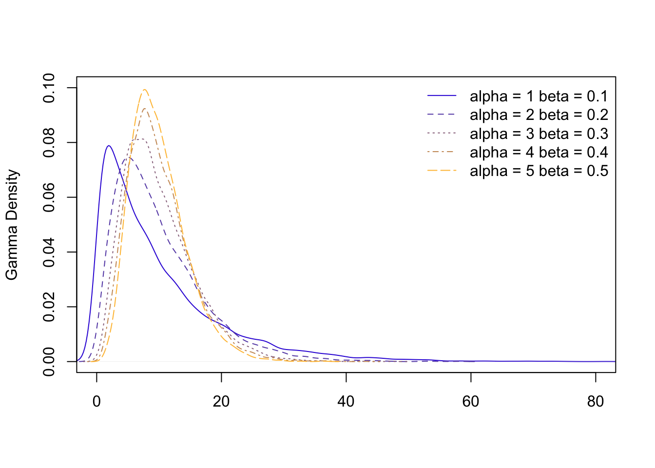
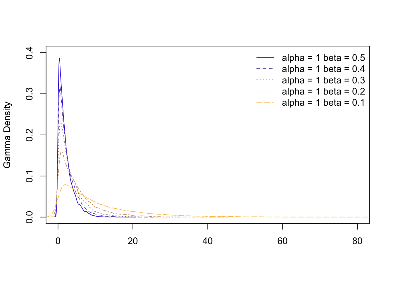
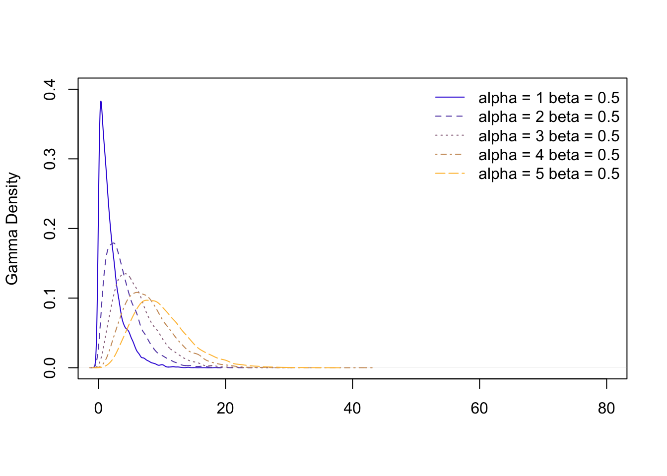
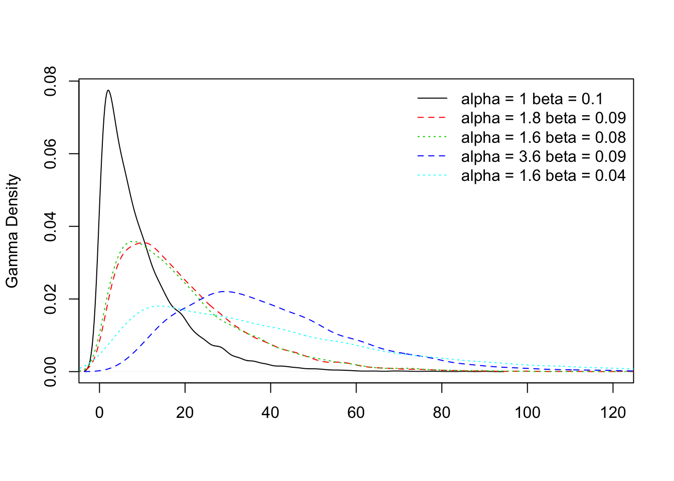
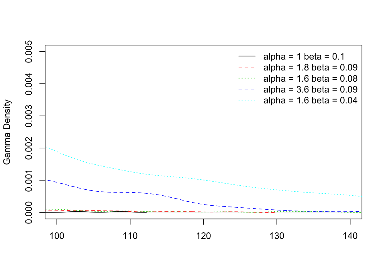
Figures 1 show some possibilities for altering $\alpha=\sum\alpha_{i}$ and $\beta$ in order to give an integrated insight of the roles of $\alpha$ and $\beta$ in growth and inequality. From the figures, one can easily distinguish the contributions made by $\alpha$ and $\beta$ to inequality in a dynamical setting. Figure 1(a) by holding the same mean value, increasing both $\alpha$ and $\beta$ shifts the center to the right. Although percentages in the high value states reduce, more is gained as the percentages in the low value states reduce more significantly. Figure 1(b) considers changes of $\beta$. By reducing $\beta$ from $0.5$ to $0.1$, we can see more and more probabilities tend to be in the high value states. However, the changes for low value states are not so significant. Figure 1(c) considers the same initial position as (b) then we increase the values of $\alpha$. The final position of the dynamics share the same mean as the final one in (b). However, the whole shape of the distribution moves more significantly to the right. The movements around the low value regions are much more significant than those happened for $\beta$, even though the changes of means are the same. Figures 1(d) and (e) consider increasing $\alpha$ and decreasing $\beta$ simultaneously but in different scales. By holding the same means, one trend is to increase more $\alpha$ the other is to decrease more $\beta$. For subtle changes, $(\alpha=1.8,\beta=.09)$ and $(\alpha=1.6,\beta=.04)$, the effects are quite similar. But if we amplify the trends, we can see that an increase of $\alpha$ eliminates larger percentages of lower value states than a decrease of $\beta$, moreover, the decrease of $\beta$ attributes more probabilities to very high value states.

If we consider the value of states below $20$ as poor status, Figures 1(b) and (c) demonstrate that increasing $\alpha$ can more efficiently reduce the poverty percentage. It means that encouraging individuals to make significant contributions to the aggregate growth can be helpful to reduce the inequality issue of the economy. To summarize these figures, the role of $\alpha$ emphasizes individual strengths that have impacts on the aggregates, the role of $\beta$ considers growth events that happen with an equivalent size $1/\beta$ across all individuals in the economy. To increase the mean of stationary aggregates, one can think of increasing $\alpha$, decreasing $\beta$ or doing both. From the dynamical patterns in Figure 1, one can see that within the same magnitude of mean value changes, $\alpha$ plays a more important role in reshaping the distribution structure.

6.3 Equality Paradox

Previous discussions and examples of Gamma distributions suggest that increasing $\alpha$ can more efficiently reduce the poverty percentage than decreasing $\beta$. It suggests that encouraging individuals to make significant contributions to the aggregate growth can be more helpful to reduce the inequality issue even though equivalently increasing possible growth size for all individuals seems more fair at first glance. As change of $\beta$ refers to an equality strategy, it is counter-intuitive to think that an economic growth by reducing $\beta$ may arise inequality. This is an equality paradox: an attempt of achieving equality generates inequality.

Increase of $1/\beta$ in fact only matters when growth event happens. For example, increasing returns to all inventions only matters to those who have made an invention, however everyone has a probability of inventing something thus this policy is supposed to be beneficial to everyone. What hidden in paradox is that it emphasizes the equality of opportunity and returns (everyone has the same law and everyone has the same return if the event happens) but it does not mention the distortion of opportunities for individuals. Since the size of individual growth events increase for everyone, those who are in the motion of growing will have bigger improvements of their states. Even if this movement has so little effect to the others that $\alpha$ remains the same, the economy could become more unequal. Because those who seize the opportunities will get bigger returns but those who have no opportunity in this round will face the same situation in the future. If this trend continues, namely winners get more and losers keep the same expectation, inequality will be enlarged.

Things could get worse, if the trend of increasing $1/\beta$ happens unconsciously. In this model, the evolution of economy automatically admits new labor forces with the same stochastic production patterns as the existing ones. By scaling property of $\mathbb{P}$-laws, it implies an increasing trend of $1/\beta$ along this evolutionary path. Additionally, a policy that is intended to meet social moral criteria often claims more for equality meanwhile economic instruments of the policy are often intended to use rewards as incentive plans. So $1/\beta$ increases. In the process, people may not even realize their actions of generating inequality. It is even harder to perceive the trend if the whole economy is in an expansion. When the effect of decreasing $\alpha$ is compensated by increasing $1/\beta$, the mean $\alpha/\beta$ can still be the same as before or even higher. Thus one should be aware that some parts of the growth caused by $\beta$ may be a sacrifice of the value $\alpha$. This tendency is shown clearly in Figures 1(d) and (e). Higher $1/\beta$ increases the percentage of upper and upper middle class but the poor almost remain the same as before. New upper and upper middle class consist mainly of those from the previous middle class.

6.4 Conjectural Strips

Corollary 4.

If $X_{t}(\omega)$ reaches stationary, $c=x$ and $\mathbb{W}(x|x^{\prime})\equiv 0$ degenerates, (5) becomes

$$x\frac{d\mathbb{P}(x)}{dx}=\alpha\mathbb{P}(x)$$ (9)

whose solution is $\mathbb{P}(x)=\mathbb{P}(1)x^{-\gamma}$, a power law distribution with parameter $\gamma=\alpha^{-1}$.

Corollary 4 gives a continuous version of the model used in [10] where the power law comes from a difference equation. For more discussion about power law and its applications in economics, please refer to the survey [5]. From Corollary 4, one can easily obtain the Riemann Zeta distribution. A short description is given in Appendix B.5.

The Zeta distribution from (9) and the Gamma distribution from (6) can be connected by the Riemann functional equation

$$\zeta(s)=2^{s}\pi^{s-1}\sin\left(\frac{s\pi}{2}\right)\Gamma(1-s)\zeta(1-s).$$ (10)

It connects the Riemann Zeta function $\zeta$ from the denominator of the Zeta distribution and the Gamma function $\Gamma$ from the denominator of the Gamma distribution. Equation (10) can have multiple zeros at those $s=-2,-4,\dots$ such that $\sin(s\pi/2)=0$. These are called trivial zero of Zeta function. As the Zeta distribution is not defined for negative $s$, we can only consider the corresponding Gamma distributions at $\alpha=3,5,7,\dots$. Suppose that there are two connected systems, one is an equilibrium economy with stationary Gamma distribution from (6), the other one with an equilibrium characterized by a Zeta function $\zeta$. Assume that these two systems are connected by the same parameter $\alpha$. When $\alpha=3,5,\dots$, although the economy has stationary solutions, the other system faces zeros of $\zeta$. If this $\zeta$ is the denominator of an equilibrium solution, such as $\zeta$ in the Zeta distribution of (9), then the other system is arriving at a singular point. In this case, even $\alpha$ does not cause any significant change for the economy, economy may confront some shocks from the other system.

Another hypothesis to consider is the case of $s=1/2$. At $s=1/2$, equation (10) gives a unique result of $\Gamma(1/2)$ which is $\sqrt{\pi}$. Moreover, Stirling’s formula gives a useful recurrence form for $\sqrt{\pi}$ that relates to $\Gamma(\cdot)$

$$\Gamma\left(k+\frac{1}{2}\right)=\Gamma\left(\frac{1}{2}\right)\cdot\frac{1}{2}\cdot\frac{3}{2}\cdot\dots\cdot\frac{2k-1}{2}=\sqrt{\pi}\cdot\frac{(2k)!}{2^{2k}k!}.$$

Since $\pi$ often refers to a stable and harmonic state, a natural question is whether these values have meanings for economic dynamics? Does $\pi$ affect the economic activities? Does an economy tend to stay in a growth path with $\alpha=k+1/2$ such as $\alpha=3/2,\dots$ rather than other values? Here is a conjecture: $\alpha$ that indicates the vigor of an economy has some critical values, some values may cause singular effects in the related systems, some values may establish stable states that are difficult to pass over. These values could be the critical strips for the growth of human beings.

7   Growth and Inequality in U.S. 1994-2015

Two data sets are used for the illustration. For growth, the data information comes from U.S. real GDP per capita issued by the U.S. Bureau of Economic Analysis. It is a quarterly data set available from $1947$ to the present. For personal income, the data comes from Current Population Survey (CPS) issued by the U.S. Bureau of Labor Statistics and the Census Bureau. We choose the category that records personal total money income from persons of $15$ years old and over. Both data sets are public and available on-line. Time period from $1994$ to $2015$ is selected to make the time range of two data sets comparable.

Estimates are divided into two parts. The first part considers the reduced form mean field system that is developed in (4). Aggregate GDP is assumed to stochastically follow $\mathbb{Q}$-law and its realization is $m_{Y}(t)$. The main interest is to capture non-stationary dynamics of $\mathbb{Q}$. We estimate the parameters that specify the dynamics of the first two moments of $\mathbb{Q}$. The second part considers the structural form system that is developed in (7). Income distribution is treated as an equilibrium aggregate solution following $\mathbb{P}$-law. A structural relationship between GDP and income distribution is exploited. We first estimate structural parameters that characterize $\mathbb{P}$-law and then use them to make a further estimate for the time varying parameters that characterize $\mathbb{Q}$-law. The structural relationship between income and GDP data eliminates an endogenous effect that is shown in the regression pre-analysis. The scheme of both estimates is given in Appendix B.6.

First, let $m_{Y}(t)$ in (4) represent the realized GDP per capita in year $t$. The continuous time representation of (4) needs to be discretized for time series data and its regression analogy is given as follows

$$m_{Y}(t+1)-m_{Y}(t) =\mbox{Constant}+\mbox{Coef}_{1}m_{Y}(t)+\mbox{Coef}_{2}\sigma_{Y}^{2}(t)+\varepsilon_{t}$$ (11)

$$\sigma_{Y}^{2}(t+1)-\sigma_{Y}^{2}(t) =\mbox{Constant}+\mbox{Coef}_{3}m_{Y}^{2}(t)+\mbox{Coef}_{4}\sigma_{Y}^{2}(t)+\upsilon_{t}$$ (12)

where $\varepsilon_{t}$, $\upsilon_{t}$ are assumed to be white noise. The variance $\sigma_{Y}^{2}$ is constructed by the residual from a pre-estimate of (11) without $\sigma_{Y}^{2}$. The model shares some similarities with the conditional heteroskedasticity models in statistics and econometrics such as the class of (generalized) autoregressive conditional heteroskedasticity (GARCH) models. As $Y_{t}(\omega)$ is generated by nonlinear function $g(\cdot)$, one would expect severe heteroskedasticities caused by $g(\cdot)$. This concern is well understood in the statistics literature. But there are two crucial differences. First, the variance term $\sigma_{Y}^{2}(t)$ does not relate to the noise $\varepsilon_{t}$. It is the higher order information term from the expansion of mean field equation while in heteroskedasticity models $\sigma_{Y}^{2}(t)$ represents the variance of the noise. Second, as $\sigma_{Y}^{2}(t)$ is an expansion term, it also depends on the mean field function $m_{Y}(t)$. This never happens in heteroskedasticity models. These two differences are reflected by the coefficient of $\sigma_{Y}^{2}(t)$ in (11) and the coefficient of $m_{Y}^{2}(t)$ in (12).

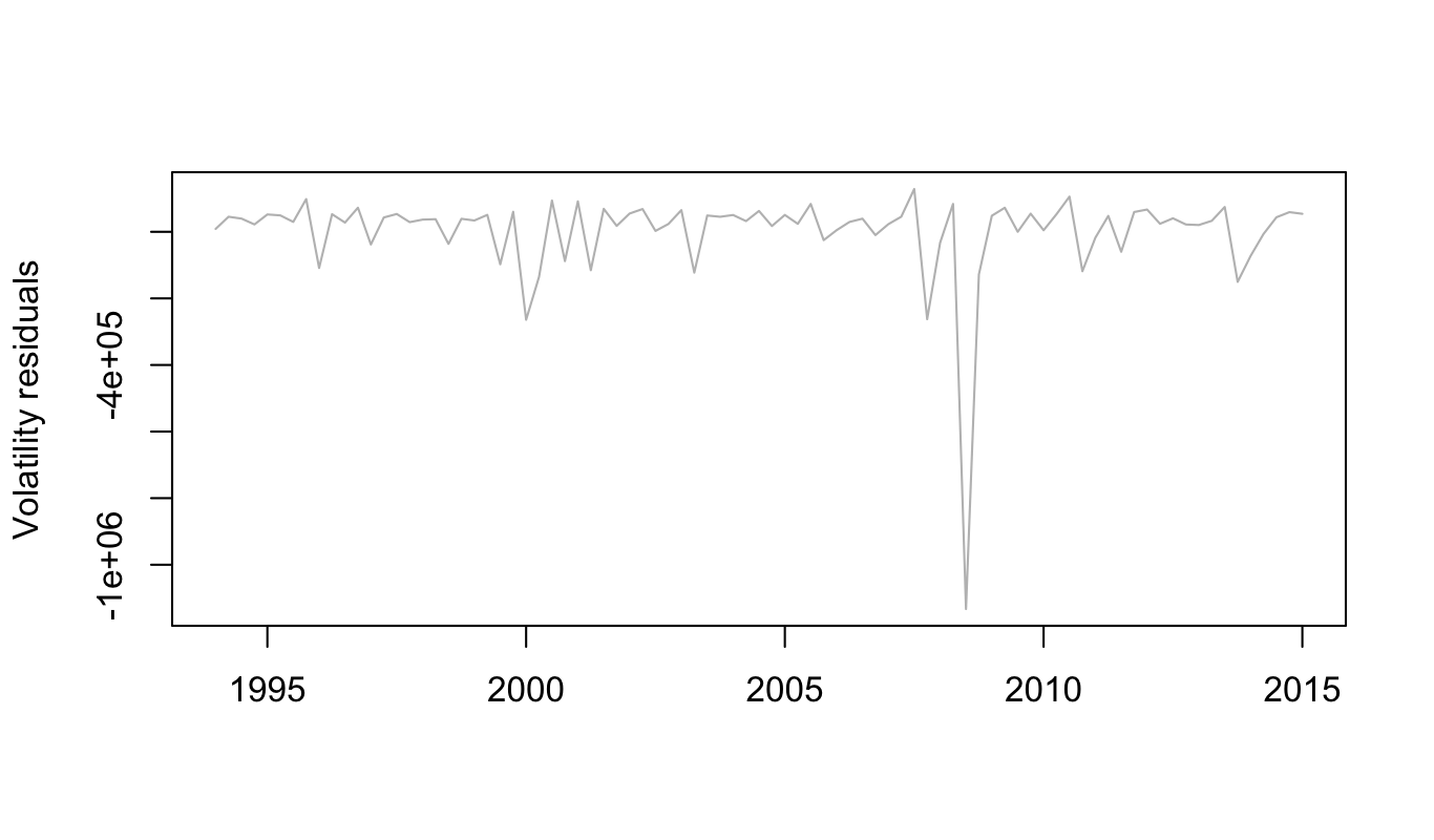
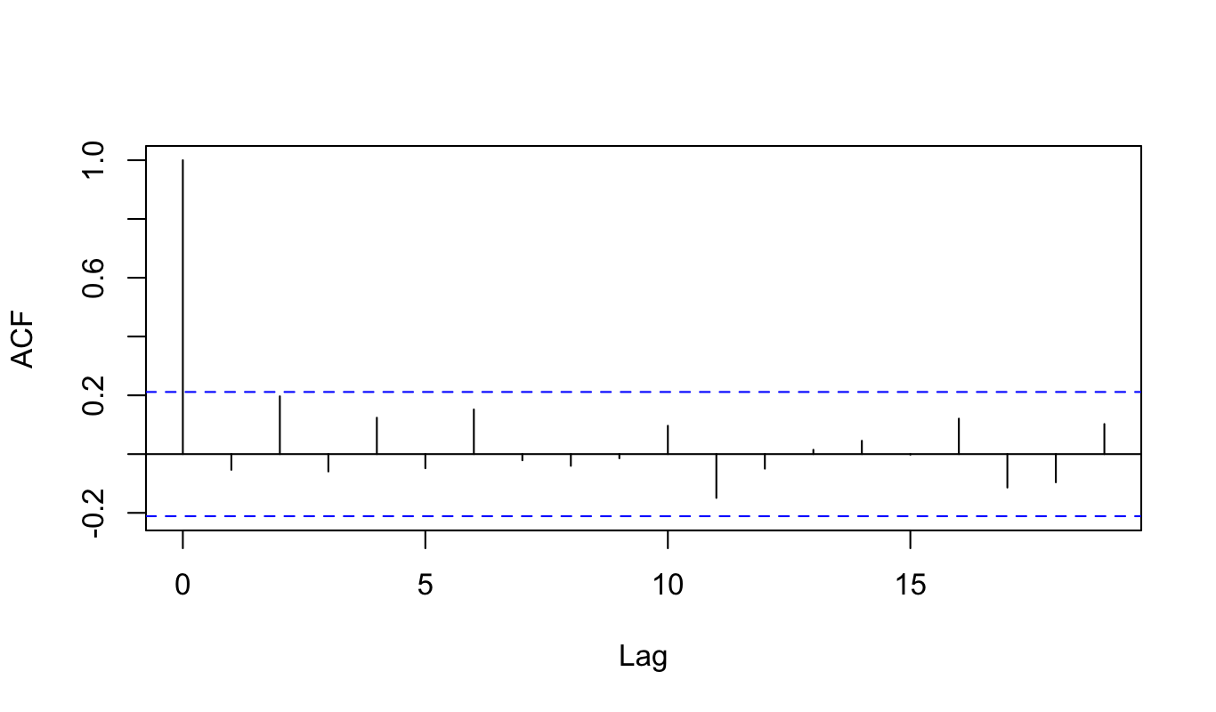
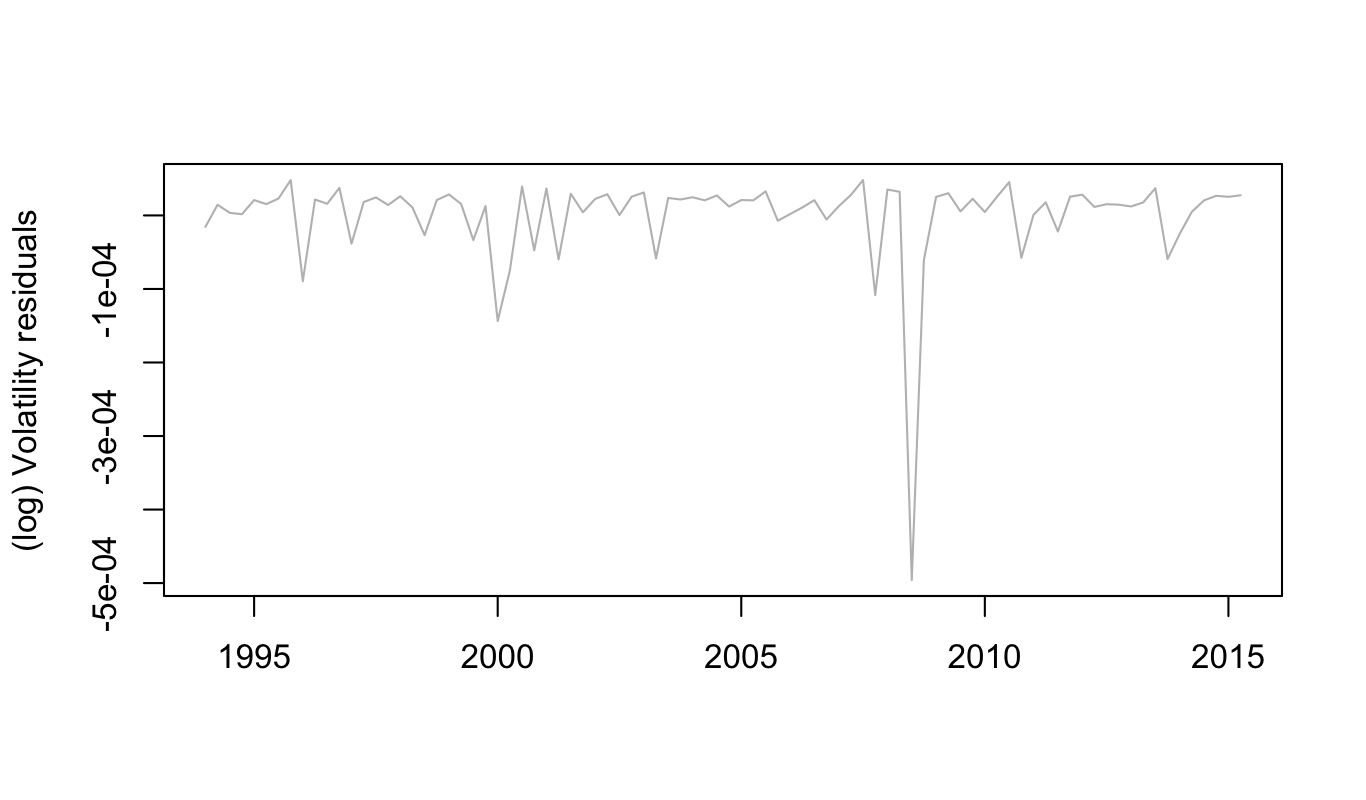
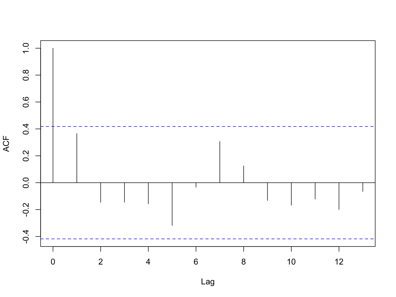
Estimate results for for (11) and (12) are given in Table LABEL:Tab:RF. The results contain two cases. One uses GDP as the mean field growth variable $m_{Y}(t)$ the other one uses logarithm of GDP as the mean field growth rate. From the table, we can see the coefficients of $\sigma_{Y}^{2}(t)$ in (11) and (12) are all significant which means the mean field dynamics $dm_{Y}(t)$ is correlated with the higher order information from its volatility $\sigma_{Y}^{2}(t)$. The residual plots for both cases are given in Figure 2 and 3 respectively. All residual look stationary. However, the residuals in (12) some dependent structure remains. This may be due to the large perturbation around $2008$.

For structural estimation of (7), some specification of non-linear function $g(\cdot)$ is pre-required. For simplicity, it is assumed that $g(\cdot)$ is an exponential function and (5) is stationary so that $\sum_{i=1}^{N}X_{t}(\omega^{i})\sim\mbox{Gamma}(\alpha_{t},\beta_{t})$. The income distribution therefore is a stationary outcome but the parameters $(\alpha_{t},\beta_{t})$ as endogenous variables adjust to the new level each year due to the interaction and evolution effects of the aggregation. The estimation form is given as follows

$$\mathbb{E}\left[\sum_{i=1}^{N}X_{t}(\omega^{i})\right] =\frac{\alpha_{t}}{\beta_{t}}=\mbox{Cons}+\mbox{Coef}_{1}\times\ln m_{Y}(t),$$ (13)

$$\ln m_{Y}(t+1)-\ln m_{Y}(t) =\theta(t)+\varepsilon_{1,t}+\frac{\varepsilon_{2,t}}{\sum_{i=1}^{N}X_{t}(\omega^{i})},\quad\varepsilon_{i,t}\sim GWN(0,1).$$ (14)

The assumption of Gaussian white noises for $\varepsilon_{1,t}$ and $\varepsilon_{2,t}$ and the simplification of $e_{t}/m_{Y}(t)$ in (8) are purely due to technical purposes. Because assuming linear additive Gaussian structure can give us a feasible filtering algorithm. In the estimation, we use the forward filtering part of the Baum-Welch formula. For details, please see Appendix B.7.

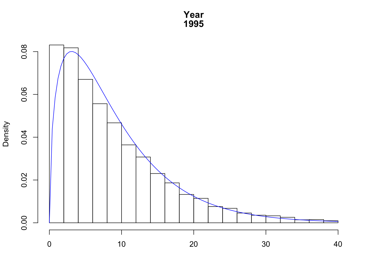
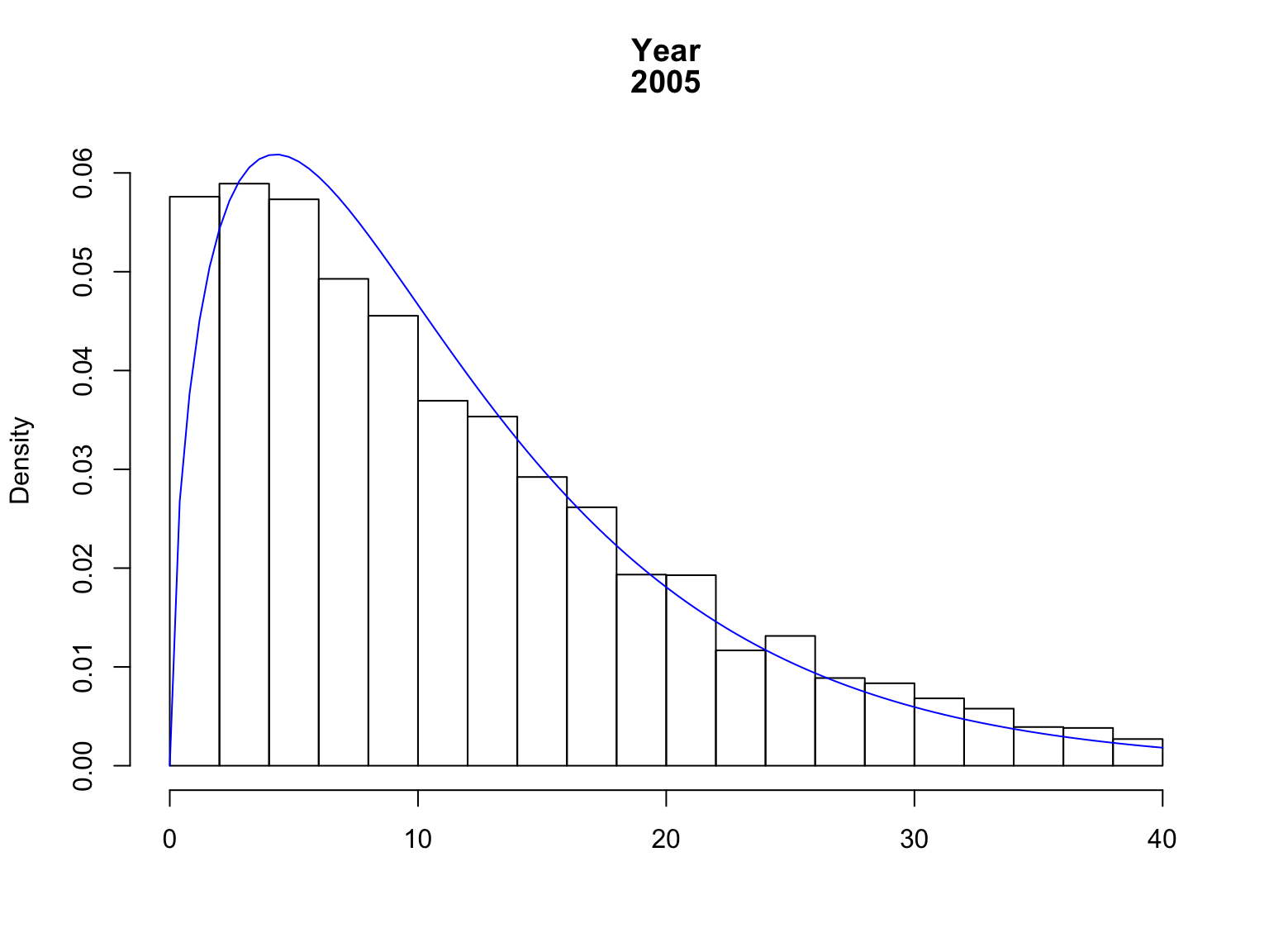
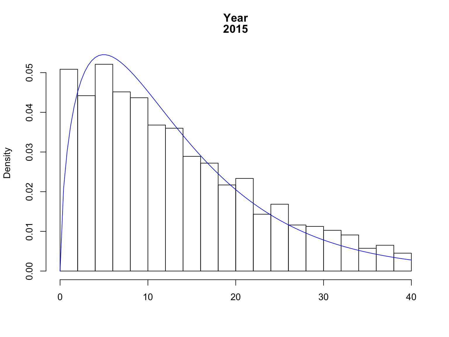
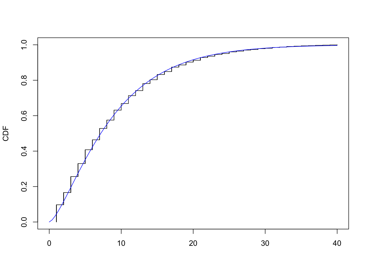
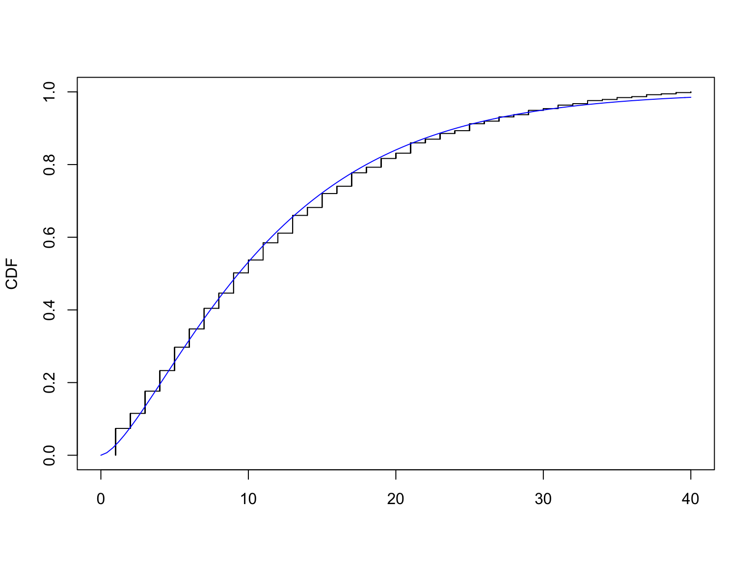
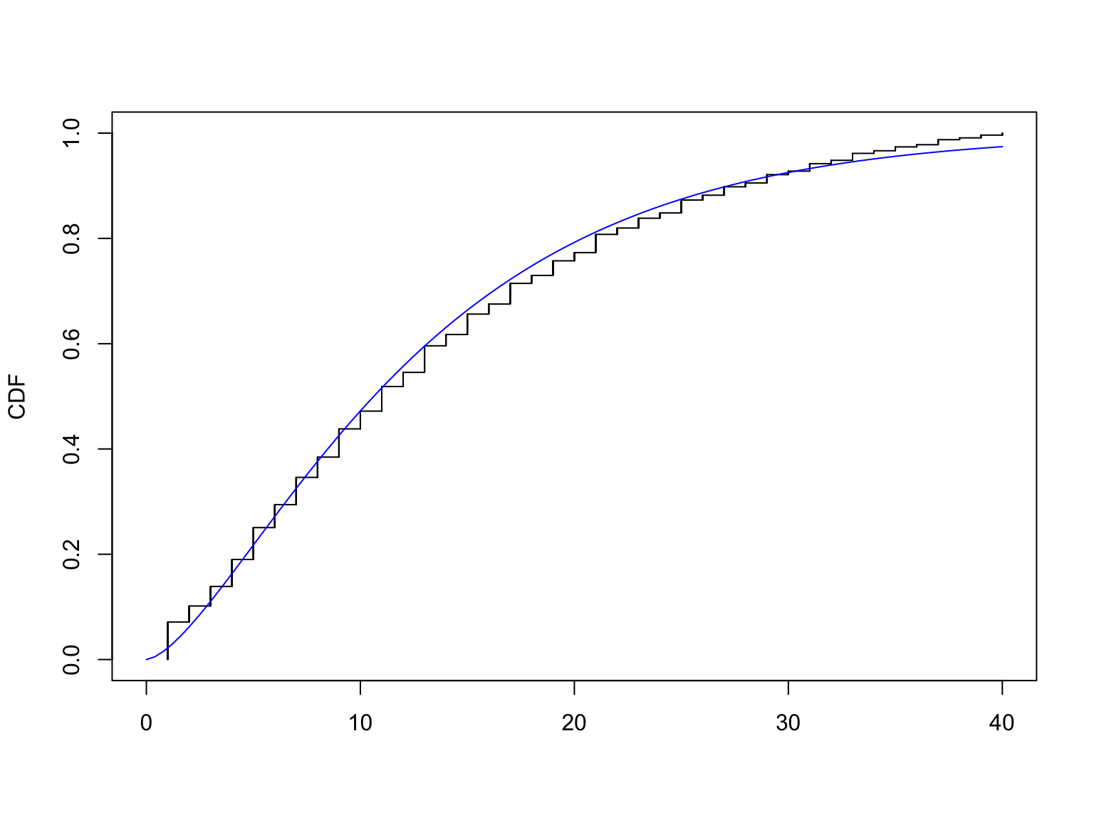
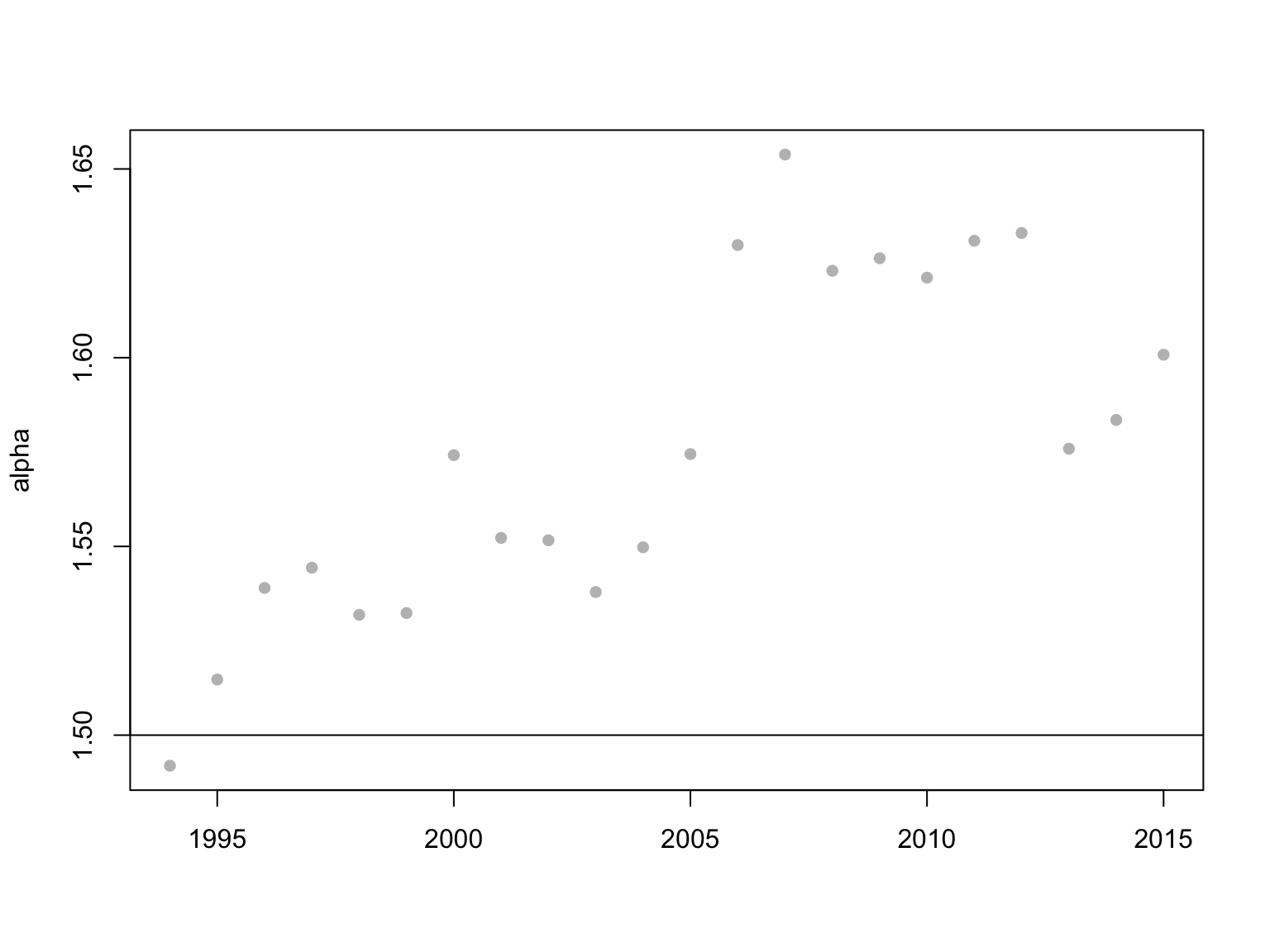
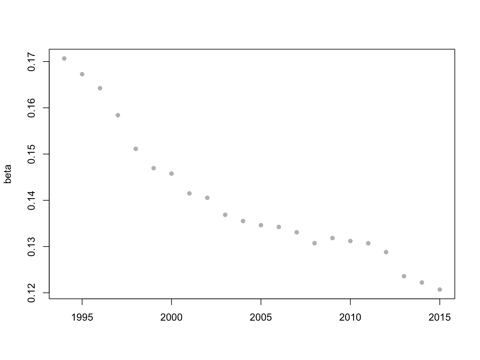
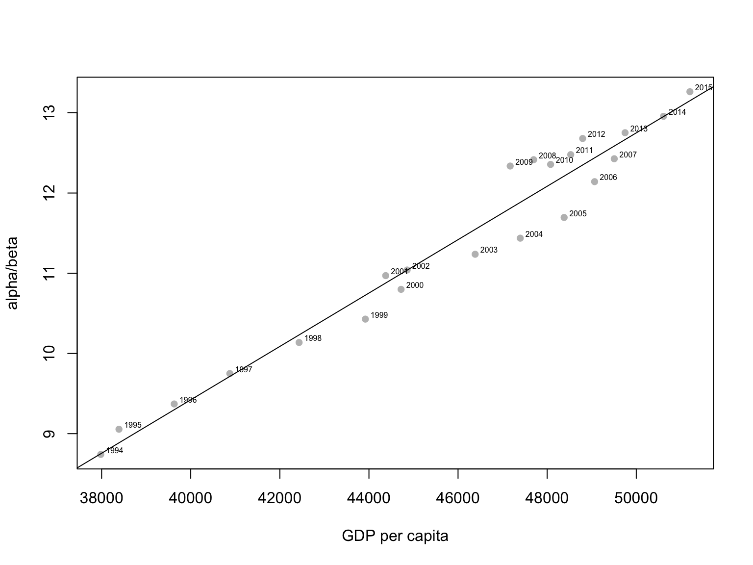
The full estimation is divided into two steps. First, we need to estimate $(\alpha_{t},\beta_{t})$ using income data from $1994$ to $2015$. Figure 4 shows three selective years for illustration. The plots show the Gamma specification fits well with both density and cumulative distribution function. The plots for other years provide similar results that can be found in the online appendix. Dynamical patterns of $(\alpha_{t},\beta_{t})$ can be found in Figure 5. The trend of $\alpha_{t}$ is increasing but it has fluctuations around late $1998$, $2003$, $2008$ and $2012$ which correspond to early $2000$s recession and financial crisis of $2008$. It is surprising that the drop at $2012$ has a bigger scale than that of $2008$. The trend of $\beta_{t}$ is monotone decreasing. It drops about $30\%$ (from $0.17$ in $1994$ to $0.12$ in $2015$). According to this calculation, the scale of $\beta$ decreasing contributes more to the growth than the increase of $\alpha$. This argument can be verified in Figure 6(a) where it shows an almost linear trend between GDP and $\alpha_{t}/\beta_{t}$, the mean of Gamma distribution. U.S. GDP keeps growing since $1994$. However if we compare this result with the trends of $\alpha_{t}$ and $\beta_{t}$, we can see the growth may be mostly from the decline of $\beta$ value. From the arguments in Section 6.2, we can see these phenomena may imply an enlarged inequality happening in U.S..

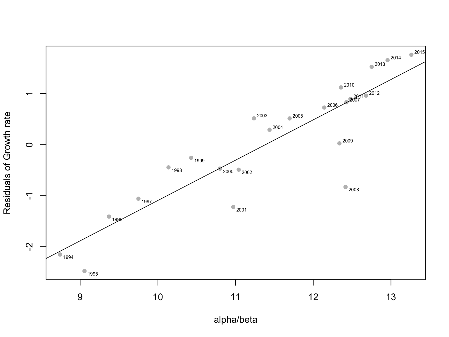
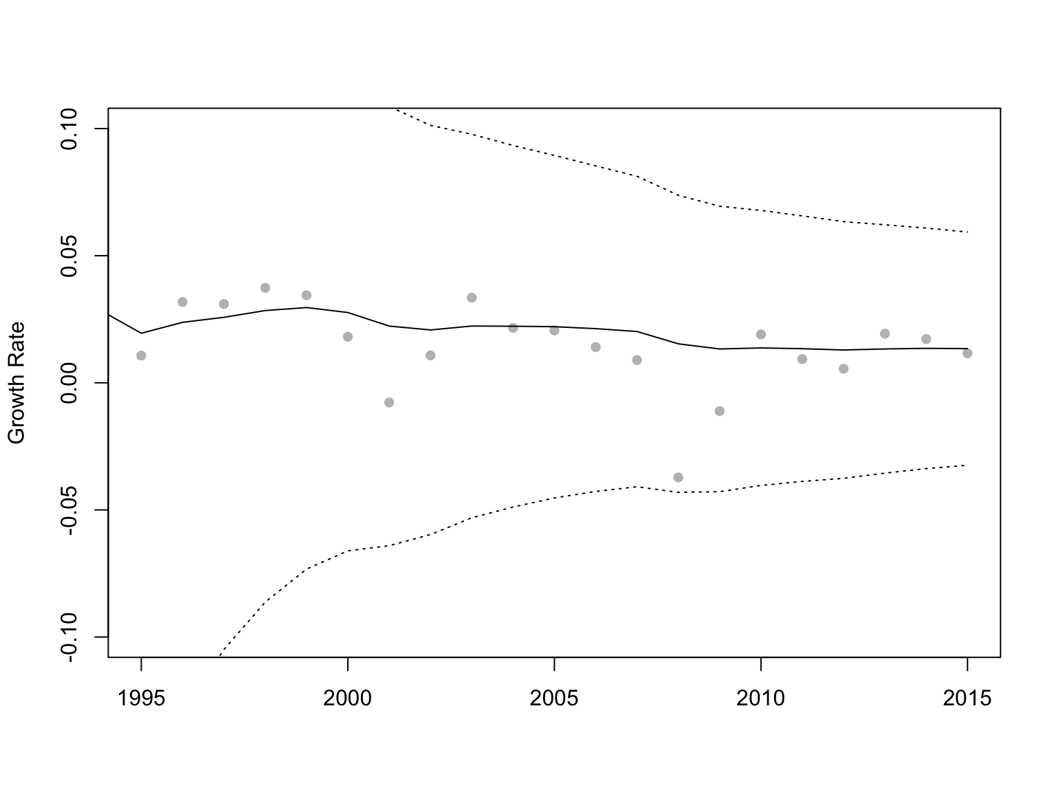
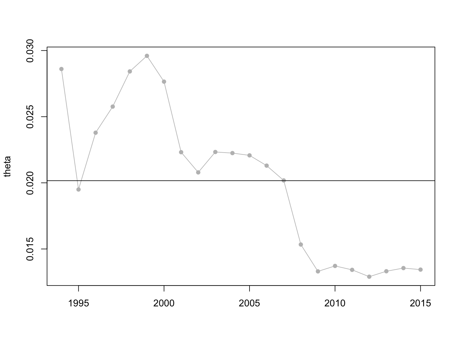
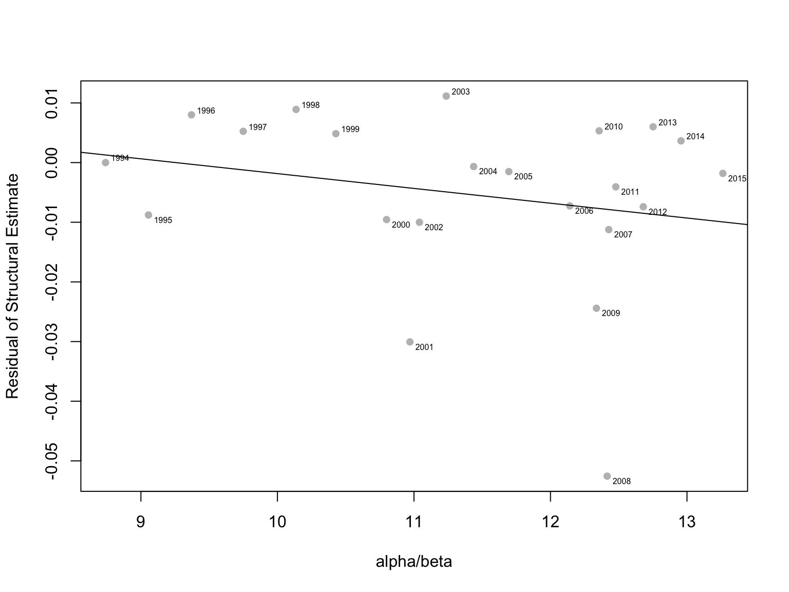
With estimated $(\alpha_{t},\beta_{t})$, the second step is to estimate equations (13) and (14). The results are given in Table 2. The first result is from a regression of $m_{Y}(t)$ on $\alpha_{t}/\beta_{t}$. It shows a significant relation that coincides with Figure 6(a). Equation (13) also has a significant coefficient. However, $\alpha_{t}/\beta_{t}$ is shown to have a significant correlation with the residual of (13) that implies an endogenous issue of (13). Figure 6(b) also illustrates this problem. With this concern, we give a structural estimate of equation (14). First we filter out the effect of $\theta(t)$ then by using the information of the variance $\alpha_{t}/\beta_{t}^{2}$ of Gamma distribution, we remove the heteroskedasticity effect. The residual of this estimate as shown in the in Table 2 is uncorrelated with $\alpha_{t}/\beta_{t}$. Figure 7(a), (c), (d) show that forward filter estimate has captured the heteroskedasticity and that its residual is stationary and uncorrelated with $\alpha_{t}/\beta_{t}$.

The estimated values of time varying parameter $\theta_{t}$ can be found in Figure 7(b). By extracting high order information interacting with the income distribution, dynamical pattern of $\theta$ gives us a very different picture about recent growth in the U.S.. As we have seen in Figure 5, the growth of stationary aggregates $\alpha_{t}/\beta_{t}$ is mainly intrigued by reducing $\beta_{t}$. The decrease of $\beta$ contributes to the GDP growth thorough the non-linear aggregation. Once we extract these stationary and non-stationary effects, the filtered growth rate of U.S. GDP is significantly decreasing after $2003$ and it remains at a relatively low level. Although Figure 7(b) gives a different dynamical patterns from the existing figures of U.S. GDP growth rate, the mean of this structural parameter, $0.02$, is close to the averaged official figures. This closeness results from the economic expansion in late 90s.

Overall, these empirical results give interesting alternative interpretations to the recent development in the U.S.. We need to emphasize that these empirical estimates have make some simplifications from the theoretical models. These simplifications so far have not generated unrobustness. But we expect more sophisticated approaches to improve these estimates.

8   Bird’s-eye View

8.1 Deterministic and Stochastic Economies

Section 3 and 4 discuss two different types of economies. It is obvious that the stochastic economy is more realistic and closer to the economy where we live. On the other hand, deterministic economy describes an illusion that is closer to the utopian images where there is no unequal status and people produce ample goods. If we want our society to evolve to a utopian state, can this deterministic economy be the destination of this evolution sequence?

To reach this destination, the deterministic economy needs to reach the same level of production as the stochastic one. That is to say, the deterministic individual growth function $f(\cdot)$, need to produce as much as the stochastic counterpart $f^{(a)}(\cdot)$ does. Unfortunately, the functional class of $f$ is smaller than that of $f^{(a)}$ which means $f$ cannot incorporate with some growth patterns that are feasible under $f^{(a)}$. In fact, $f$ can be a special case of $f^{(a)}$ where $a$ is a deterministic sequence indexing every period of time. Even for deterministic function, $f$ can not be embedded in many interesting cases. For example, some deterministic logistic maps or cobweb models can be ruled out from the class of $f$, because they can induce infinite many bifurcations that give the randomness to the growth.

Another important point is that in the evolution process variation happens in an uncertainty way, at least, to our best understanding so far. Innovations and their external effects are rather crucial to our growth and evolution but they are unpredictable. Thus instead of viewing deterministic economy as a utopia limit of our evolution, it is better to think it as the garden of Eden, the initial state of a stochastic economy from which the uncertainty appeared.

8.2 Nonlinearity

Section 5 points out the difference between stationary and non-stationary aggregates. As non-stationarity comes from nonlinear aggregation functions, one concern is the role of non-linearity. It is well known that many nonlinear patterns can be found in population growth, urbanization, social interactions, etc. All these nonlinear processes in some senses seem to increase our productivities. Meanwhile, these processes also cause many problems.

The same dilemma can be found in the model in Section 5. It shows that uncertainty level is propagated by nonlinearity. Volatility or even higher order information may contribute to the final aggregation. Laws of individual or stationary aggregates are distorted during the nonlinear aggregation. One can infer that the higher the nonlinearity, more severe the distortion is. It is not so clear the total effect of this type of distortion. We know the innovation is highly unpredictable, so we tend to believe that the likelihood of innovation is higher in a nonlinear agglomeration. But the occurrences of war and crisis also reflect some nonlinear features, can we believe that non-stationary aggregations also conspire these events? If non-stationary aggregation accompanies with both angels and evils, it is our duties to prevent the worst case scenarios.

8.3 $\alpha$-Growth and $\beta$-Growth

Section 6 uses $(\alpha,\beta)$ to connect individual probabilistic laws and aggregates’. It points out the different roles of $\alpha$ and $\beta$ in determining inequality. The growth driven by $\alpha$ tends to create a more equal economy than the one driven by $\beta$. A policy maker should be in favor of proposals that may increasing $\alpha$ rather than decreasing $\beta$.

However, $\alpha$ and $\beta$ are deeper parameters that can be embedded in people’s characters (risk loving or risk aversion), social norms (conservative or liberal), or even culture and religion (creative and independent or stable and united). The direct policy on income or wealth may hardly affect these intrinsic characters making up of $(\alpha,\beta)$. For example decreasing $\beta$ can be an unconscious action as shown in the equality paradox in Section 6. The core of this paradox is that $\beta$ is uncorrelated with $\alpha$ and decreasing $\beta$ happens naturally in the evolution of the economy. So far it is hard to identify the connection between $\alpha$ and $\beta$. Thus the way of drafting a policy to support $\alpha$-growth is in the mist. Deeper policy that can affect these parameters may relate to some fundamentals of society such as education and religious systems.

An economy of considering only $\beta$-growth could be in danger. When $\beta$ becomes small enough, the economy will become highly unequal. In this case, even if the economy scale can reach to a very high level (by assuming $\alpha$ not decreasing), the structure is fragile because the majority concentrate on one side and they are far from the elites whose fraction of the population decreases with $\beta$. This type of social structure often leads to a revolution, a war, or a creative destruction. Should we need to resist a $\beta$-growth? If yes, then how?

9   Conclusive Remarks

A new perspective, new laws, and new models are proposed. Meanwhile, a new paradox, new challengings and new expectations are initiated. Lights are shining onto an unfamiliar and perhaps treacherous direction that however can not and should not be concealed. Effective work in this direction necessarily calls for a shift from classical devices to novel ones. New theories deal simultaneously with heterogeneity, endogeneity, and dynamics. New interpretation considers to treat the nature, the forces and the human factors that determine the characteristics and trends of our evolution as a whole. New machineries integrate these complexities in reality and are ready for a venture into fields beyond recognized patterns. A fascinating risk awaits in front. But one intuition becomes clear. Growth and inequality, two symbiosis contraries in the names of goodwill and “evil”, will float with us towards the brave uncertain new world, that has such people expecting it.

(a) Mean invariance

(b) Variations of $\beta$

(c) Variations of $\alpha$

(d) Variations of $(\alpha,\beta)$

(e) Variations of $(\alpha,\beta)$ in the tail

Figure 1: Gamma Distribution

Table 1: Results of Reduced Form Estimates

	Dependent variable:
	$m_{Y}(t+1)-m_{Y}(t)$		$\sigma_{Y}^{2}(t+1)-\sigma_{Y}^{2}(t)$
	Growth (11)	Growth rate (11)	Growth (12)	Growth rate (12)
Coef-1 $-$0.010	$-$0.016∗∗
	(0.007)	(0.007)
Coef-2	$-$0.001∗∗∗	$-$40.777∗∗∗
	(0.0002)	(8.778)
Coef-3			$-$0.00002	$-$0.00000
			(0.00005)	(0.00000)
Coef-4			0.772∗∗∗	0.780∗∗∗
			(0.107)	(0.107)
Constant	665.123∗∗	0.176∗∗	$-$7,306.789	0.00004
	(306.751)	(0.070)	(99,917.010)	(0.0004)
Observations	87	87	86	86
R2	0.281	0.254	0.386	0.390
Adjusted R2	0.264	0.236	0.371	0.375
Residual Std. Error	240.671 (df = 84)	0.005 (df = 84)	145,910.300 (df = 83)	0.0001 (df = 83)
F Statistic	16.404∗∗∗ (df = 2; 84)	14.308∗∗∗ (df = 2; 84)	26.036∗∗∗ (df = 2; 83)	26.535∗∗∗ (df = 2; 83)
Note:	∗p$<$0.1; ∗∗p$<$0.05; ∗∗∗p$<$0.01

(a)

(b)

(c)

(d)

Figure 2: Residuals in Reduced Form Estimate (Growth)

(a)

(b)

(c)

(d)

Figure 3: Residuals in Reduced Form Estimate (Growth rate)

Table 2: Results of Structural Form Estimates

	Dependent variable:
	$\alpha_{t}/\beta_{t}$		Residual of	Residual of
	pre-analysis	(13)	(13)	(14)
$m_{Y}(t)$	0.0003∗∗∗
	(0.00002)
Coef-1		$-$35.695∗∗
		(15.500)
$\alpha_{t}/\beta_{t}$			0.790∗∗∗	$-$0.002
			(0.091)	(0.002)
Constant	$-$3.891∗∗∗	11.916∗∗∗	$-$8.999∗∗∗	0.023
	(0.712)	(0.348)	(1.043)	(0.027)
Observations	22	22	22	22
R2	0.959	0.210	0.790	0.051
Adjusted R2	0.957	0.170	0.780	0.003
Residual Std. Error (df = 20)	0.279	1.220	0.559	0.015
F Statistic (df = 1; 20)	464.048∗∗∗	5.303∗∗	75.425∗∗∗	1.071
Note:	∗p$<$0.1; ∗∗p$<$0.05; ∗∗∗p$<$0.01

(a)

(b)

(c)

(d)

(e)

(f)

Figure 4: Estimates of Income Distribution by Gamma$(\alpha_{t},\beta_{t})$

(a)

(b)

Figure 5: $(\alpha_{t},\beta_{t})$ in $1994-2015$

(a)

(b)

Figure 6: Dynamics of $\alpha_{t}/\beta_{t}$ and GDP

(a)

(b)

(c)

(d)

Figure 7: Structural Estimate

Appendix A Proofs

A.1 Proof of Lemma 1

Proof.

We know that $X_{t}(\cdot)=f^{(a_{t})}f^{(a_{t-1})}\cdots f^{(a_{1})}(\cdot)$ and that $(a_{1},\dots,a_{t})$ are i.i.d.. $X_{t}$ and $a_{t}$ generate the same $\sigma$-algebra $\mathcal{B}_{t}$. Then for any $a^{\prime}_{t-2}\in\mathcal{B}_{t-2}$, $a_{t-2}^{{}^{\prime}}$ and $a_{t}$ are independent, so

$$\Pr\left\{X_{t}\in A\left|a^{\prime}_{t-2},\>X_{t-1}\right.\right\}=\Pr\left\{f^{(a_{t})}(X_{t-1})\in A\left|a^{\prime}_{t-2},\>X_{t-1}\right.\right\}=\Pr\left\{f^{(a_{t})}(X_{t-1})\in A\left|X_{t-1}\right.\right\}$$

which is the Markov property $\Pr\{X_{t}\in A|\mathcal{B}_{t-1},\mathcal{B}_{t-2}\}=\Pr\{X_{t}\in A|\mathcal{B}_{t-1}\}$. The result follows. ∎

A.2 Proof of Lemma 2

Proof.

Assumption 5 implies that we can select a subsequence $\{a_{t}^{{}^{\prime}}\}\subset\{a_{t}\}$ so that $\tilde{X}_{t}(\cdot)=f^{(a_{t}^{{}^{\prime}})}(\cdot)$ and $\tilde{X}_{t}(\cdot)$ is monotone. We have $\tilde{X}_{t}(\underline{\Omega})\leq\tilde{X}_{t+1}(\underline{\Omega})$ almost surely. Then given $y$, we have $\Pr(\tilde{X}_{t}(\underline{\Omega})\leq y)\geq\Pr(\tilde{X}_{t+1}(\underline{\Omega})\leq y)$. Since given $\underline{\Omega}<y<\overline{\Omega}$, $\Pr(\tilde{X}_{t}(\underline{\Omega})\leq y)$ is monotone in $t$ and $\Pr(\tilde{X}_{t}(\underline{\Omega})\leq y)$ is bounded between $0$ and $1$, we know that for each $y$, $\Pr(\tilde{X}_{t}(\underline{\Omega})\leq y)$ must converge as $t\rightarrow\infty$.

Similar argument holds for $\Pr(\tilde{X}_{t}(\overline{\Omega})\leq y)$. As $y<\overline{\Omega}$, it is obvious that $\Pr(\overline{\Omega}\leq y)=0$. Thus we have $\Pr(\tilde{X}_{t}(\overline{\Omega})\leq y)\leq\Pr(\tilde{X}_{t+1}(\overline{\Omega})\leq y)$. Monotonicity and boundedness tell that $\Pr(\tilde{X}_{t}(\overline{\Omega})\leq y)$ must converge as $t\rightarrow\infty$.

Because the index set $\mathcal{A}$ only contains i.i.d. random variables, any other sequence $\{a_{t}\}$ has the same distribution as $\{a_{t}^{{}^{\prime}}\}$, then any $X_{t}(\cdot)=f^{(a_{t})}(\cdot)$ will induce the same convergent results for $\Pr(X_{t}(\underline{\Omega})\leq y)$ and $\Pr(X_{t}(\overline{\Omega})\leq y)$. ∎

A.3 Proof of Proposition 1

Proof.

Lemma 1 shows that $X_{t}(\omega)$ is a Markov process. For a Markov process, let $P(x,\mathcal{X})=\Pr(f^{(a)}(x)\in\mathcal{X})$ be a transition probability where $a$ has the same distribution as $a_{1}$. By definition, $X_{t}(\cdot)=\overset{t-\mbox{times}}{\overbrace{f^{(a)}f^{(a)}\cdots f^{(a)}}}(\cdot)$. We have an expression of a transition probability for $t$-times

$$P^{(t)}(X_{0}=\underline{\Omega},\mathcal{X})=\int_{\Omega}P(x,\mathcal{X})dP^{(t-1)}(X_{0}=\underline{\Omega},x).$$

As $P(x,\mathcal{X})$ is a bounded, continuous and real-valued functions on $x$, by Helly-Bray theorem ($P^{(t)}\rightarrow\mathbb{P}$) and Lemma 2, we have

$$\mathbb{P}\left(X^{*}(\underline{\Omega})\in\mathcal{X}\right)=\int_{\Omega}P(x,\mathcal{X})d\mathbb{P}\left(X^{*}(\underline{\Omega})=x\right)$$

as $t\rightarrow\infty$. This means that $\mathbb{P}\left(X^{*}(\underline{\Omega})\in\mathcal{X}\right)$ is a stationary distribution. Similar argument holds for $\mathbb{P}\left(X^{*}(\overline{\Omega})\in\mathcal{X}\right)$. ∎

A.4 Proof of Theorem 2

Proof.

Given a subsequence $\{a_{t}^{{}^{\prime}}\}\subset\{a_{t}\}$, $\tilde{X}_{t}(\cdot)=f(\tilde{X}_{t-1}(\cdot))$ and $f$ is monotone, Proposition 1 shows that $\Pr(\tilde{X}_{t}(\underline{\Omega})\in\mathcal{X})$ and $\Pr(\tilde{X}_{t}(\overline{\Omega})\in\mathcal{X})$ converge. As $\Pr(\tilde{X}_{t}(\underline{\Omega})\in\mathcal{X})\geq\Pr(\tilde{X}_{t}(\underline{\Omega})\in\mathcal{X})$, we have

$$\mathbb{P}\left(X^{*}(\underline{\Omega})\in\mathcal{X}\right)\geq\mathbb{P}\left(X^{*}(\overline{\Omega})\in\mathcal{X}\right).$$

We now prove $\mathbb{P}\left(X^{*}(\underline{\Omega})\in\mathcal{X}\right)\leq\mathbb{P}\left(X^{*}(\overline{\Omega})\in\mathcal{X}\right)$.

With Assumption 6, let $\tau$ denote the time when $X_{\tau}(\underline{\Omega})$ and $X_{\tau}(\overline{\Omega})$ will enter two separated sets. Let $\tau=\inf\left\{t:\>X_{t}(\underline{\Omega})\in\mathcal{X},\;X_{t}(\overline{\Omega})\in\Omega\backslash\mathcal{X}\right\}$. This hitting time $\tau$ is random and $\Pr(\tau<\infty)=1$. Then use the transition probability $P(x,\mathcal{X})=\Pr(f^{(a)}(x)\in\mathcal{X})$ and stationary property, we have

$$\Pr\left(X_{t}(\underline{\Omega})\in\mathcal{X},\>t>\tau\right)\overset{(a)}{=} \sum_{j=1}^{t-1}\left\{\int P(x,\mathcal{X})dP(X_{t-j}(\underline{\Omega}),x|\tau=j)\right\}\Pr(\tau=j)$$

$$\overset{(b)}{\leq} \sum_{j=1}^{t-1}\left\{\int P(x,\mathcal{X})dP(X_{t-j}(\underline{\Omega}),x|\tau=j)\right\},$$

where $\overset{(a)}{=}$ comes from the iterative expression $P(X_{2}(\underline{\Omega}),\mathcal{X})=\int_{\Omega}P(x,\mathcal{X})dP(X_{1}(\underline{\Omega}),x)$ and the conditioning of $\tau$, $\overset{(b)}{\leq}$ comes from $\Pr(\tau=j)<1$ for some $j$s.

Similar approach is applied to $X_{t}(\overline{\Omega})$:

$$\Pr\left(X_{t}(\overline{\Omega})\in\mathcal{X},\>t>\tau\right)= \sum_{j=1}^{t-1}\left\{\int P(x,\mathcal{X})dP(X_{t-j}(\overline{\Omega}),x|\tau=j)\right\}\Pr(\tau=j)$$

$$\overset{(c)}{\geq} \sum_{j=1}^{t-1}\left\{\int P(x,\mathcal{X})dP(X_{t-j}(\overline{\Omega}),x|\tau=j)\right\},$$

where $\overset{(c)}{\geq}$ comes from the fact that when $t>\tau$, $X_{t}(\overline{\Omega})\in\Omega\backslash\mathcal{X}$ so $\Pr(\tau=j)=0$. Because the subset $\mathcal{X}$ is arbitrarily chosen, we can choose the set “closer” to $\overline{\Omega}$ so that $P(X_{t}(\overline{\Omega}),\mathcal{X})\geq P(X_{t}(\underline{\Omega}),\mathcal{X})$ when $t\rightarrow\infty$. Combine this result with the previous two inequalities and take $t\rightarrow\infty$ so that $\Pr\{t>\tau\}=1$, we have

$$\Pr\left(X^{*}(\underline{\Omega})\in\mathcal{X}\right)\leq\sum_{j=1}^{\infty}\left\{\int P(x,\mathcal{X})dP(X_{t-j}(\underline{\Omega}),x)\right\} \leq\sum_{j=1}^{\infty}\left\{\int P(x,\mathcal{X})dP(X_{t-j}(\overline{\Omega}),x)\right\}$$

$$\leq \Pr\left(X^{*}(\overline{\Omega})\in\mathcal{X}\right)$$

so $\mathbb{P}\left(X^{*}(\underline{\Omega})\in\mathcal{X}\right)\leq\mathbb{P}\left(X^{*}(\overline{\Omega})\in\mathcal{X}\right)$, the result follows. ∎

A.5 Proof of Theorem 3

Proof.

By Theorem 2, we know $X^{*}(\omega^{1})\overset{d}{=}X^{*}(\omega^{2})\cdots\overset{d}{=}X^{*}(\omega^{N})$. $\overset{d}{=}$ means equivalence in distribution. A simple arrangement

$$X^{*}(\omega^{1})+X^{*}(\omega^{2})-X^{*}(\omega^{2})\overset{d}{=}X^{*}(\omega^{1})$$

does not violate the equality in distribution. The distributional expression of above equality is a convolution of $X^{*}(\omega^{1})+X^{*}(\omega^{2})$ and $-X^{*}(\omega^{2})$ such that

$$\int_{\Omega}\mathbb{P}_{X^{*}(\omega^{1})+X^{*}(\omega^{2})}\left(X^{*}(\omega^{1})+x\right)\mathbb{P}_{X^{*}(\omega^{2})}(-x)dx=\mathbb{P}(X^{*}(\omega^{1}))$$

$\mathbb{P}_{X^{*}(\omega^{1})+X^{*}(\omega^{2})}$ and $\mathbb{P}_{X^{*}(\omega^{2})}$ stand for the stationary distribution functions of $X^{*}(\omega^{1})+X^{*}(\omega^{2})$ and $X^{*}(\omega^{2})$. Without loss of generality, we just consider $\Omega\in\mathbb{R}_{+}^{d}\cup\{0\}$. Note that $\mathbb{P}_{X^{*}(\omega^{2})}(-x)=0$ for $\Omega\in\mathbb{R}_{+}^{d}$ and $\mathbb{P}_{X^{*}(\omega^{2})}(0)\geq 0$ by the property of production functions. Then the convolution degenerates to

$$\mathbb{P}_{X^{*}(\omega^{1})+X^{*}(\omega^{2})}\left(X^{*}(\omega^{1})\right)=\mathbb{P}(X^{*}(\omega^{1})).$$

So $X^{*}(\omega^{1})+X^{*}(\omega^{2})\sim\mathbb{P}$. This argument can be extended to a sum of all $X^{*}(\omega^{i})$. The result follows. ∎

A.6 Proof of Theorem 4

Proof.

Given the mean field equation (3), one expands $a_{1}(y)$ around $m_{Y}(t)$ via Taylor series

$$\int a_{1}(y)\mathbb{Q}(y,t)dy=a_{1}(m_{Y}(t))+ \overset{(*)}{\overbrace{\left[\int(y-m_{Y}(t))\mathbb{Q}(y,t)dy\right]\left.\frac{\partial a_{1}(m_{Y}(t))}{\partial y}\right|_{y=m_{Y}(t)}}}$$

$$+\frac{1}{2}\left[\int(y-m_{Y}(t))^{2}\mathbb{Q}(y,t)dy\right] \left.\frac{\partial^{2}a_{1}(m_{Y}(t))}{\partial y^{2}}\right|_{y=m_{Y}(t)}+\dots$$

where $a_{1}(m_{Y}(t))=\int(y^{\prime}-m_{Y}(t))\mathbb{W}(y^{\prime}|y)dy^{\prime}$. By the definition $\int y\mathbb{Q}(y,t)dy=m_{Y}(t)$, we know $(*)$ is zero. Thus the expression becomes

$$\int a_{1}(y)\mathbb{Q}(y,t)dy=a_{1}(m_{Y}(t))+\frac{1}{2}\overset{=\sigma_{Y}^{2}(t)}{\overbrace{\left[\int(y-m_{Y}(t))^{2}\mathbb{Q}(y,t)dy\right]}}a_{1}^{(2)}(m_{Y}(t))+\dots$$

where $a_{1}^{(2)}(m_{Y}(t))$ denotes $\partial^{2}a_{1}(m_{Y}(t))/\partial y^{2}|_{y=m_{Y}(t)}$ and $\sigma_{Y}^{2}(t)$ is variance of $m_{Y}(t)$. Similarly, one can deduce the second moment of the mean field

$$\int y^{2}\frac{\partial\mathbb{Q}(y,t)}{\partial t}dy =\int\int y^{2}\left[\mathbb{W}(y|y^{\prime})\mathbb{Q}(y^{\prime},t)-\mathbb{W}(y^{\prime}|y)\mathbb{Q}(y,t)\right]dydy^{\prime}$$

$$= \int\int\left(y^{\prime 2}-y^{2}\right)\mathbb{W}(y^{\prime}|y)\mathbb{Q}(y,t)dydy^{\prime}$$

$$= \int\int\left[\left(y^{\prime}-y\right)^{2}+2y(y^{\prime}-y)\right]\mathbb{W}(y^{\prime}|y)\mathbb{Q}(y,t)dydy^{\prime}$$

$$= \int a_{2}(y)\mathbb{Q}(y,t)dy+2\int y\,a_{1}(y)\mathbb{Q}(y,t)dy.$$

As $\sigma_{Y}^{2}(t)=\int(y-m_{Y}(t))^{2}\mathbb{Q}(y,t)dy=\int y^{2}\mathbb{Q}(y,t)dy-m_{Y}^{2}(t)$, there is

$$\frac{d\sigma_{Y}^{2}(t)}{dt} =\int y^{2}\frac{\partial\mathbb{Q}(y,t)}{\partial t}dy-2m_{Y}(t)\frac{dm_{Y}(t)}{dt}$$

$$=\int a_{2}(y)\mathbb{Q}(y,t)dy+2\int y\,a_{1}(y)\mathbb{Q}(y,t)dy-2m_{Y}(t)\int a_{1}(y)\mathbb{Q}(y,t)dy$$

$$=\int a_{2}(y)\mathbb{Q}(y,t)dy+2\int(y-m_{Y}(t))\,a_{1}(y)\mathbb{Q}(y,t)dy$$

$$\overset{(a)}{=}\int a_{2}(y)\mathbb{Q}(y,t)dy+2\int\Biggl{\{}(y-m_{Y}(t))\,a_{1}(m_{Y}(t))$$

$$+\left.\left.\frac{\partial a_{1}(m_{Y}(t))}{\partial y}\right|_{y=m_{Y}(t)}\left(y-m_{Y}(t)\right)^{2}+\dots\right\}\mathbb{Q}(y,t)dy$$

$$\overset{(b)}{=}a_{2}(m_{Y}(t))+2a_{1}^{(1)}(m_{Y}(t))\sigma_{Y}^{2}(t)+\dots$$

where $\overset{(a)}{=}$ comes from a Taylor expansion of $a_{1}(y)$ around $m_{Y}(t)$ and $\overset{(b)}{=}$ comes from another Taylor expansion of $a_{2}(y)$ around $m_{Y}(t)$. Expansion terms that outvie $(y-m_{Y}(t))^{2}$ have not displayed in the expression. ∎

A.7 Proof of Theorem 5

Proof.

A heuristic proof of (I) and (II).

(I) By Assumption 8, we consider two states transition at small time interval, a monotone growth from $x^{\prime}$ to $x=1$ or to stay at position $x=0$:

$$\mathbb{P}_{\Delta t}(x=1|x^{\prime}) =\alpha\Delta t+o((\Delta t)^{2}),$$

$$\mathbb{P}_{\Delta t}(x=0|x^{\prime}) =1-\alpha\Delta t+o((\Delta t)^{2}).$$

Let $\mathbb{P}(x_{1},t)=\Pr\{X_{t}(\omega)=x_{1}\}$. Then

$$\mathbb{P}(x_{1},t+\Delta t)\overset{(a)}{=} \mathbb{P}(x_{1},t)\Pr\{X_{\Delta t}(\omega)=0|x_{1}\}+\mathbb{P}(x_{1},t)\Pr\{X_{\Delta t}(\omega)=1|x_{1}\}$$

$$= \mathbb{P}(x_{1},t)(1-\alpha\Delta t)+\mathbb{P}(x_{1},t)\times\alpha\Delta t+o((\Delta t)^{2})$$

$$\overset{(b)}{=} \mathbb{P}(x_{1},t)(1-\alpha\Delta t)+\int\mathbb{W}(x_{1}|x^{\prime})\mathbb{P}(x^{\prime},t)dx^{\prime}\times\alpha\Delta t+o((\Delta t)^{2})$$

where $\overset{(a)}{=}$ comes from transition from $\mathbb{P}(x_{1},t)$ to $\mathbb{P}(x_{1},t+\Delta t)$ and $\overset{(b)}{=}$ comes from

$$\mathbb{P}(x_{1},t)\overset{(c)}{=}\lim_{\Delta t\rightarrow 0}\int\left(\mathbb{P}_{\Delta t}(x_{1}|x^{\prime})\mathbb{P}(x^{\prime},t)\right)dx^{\prime}\overset{(d)}{=}\int\mathbb{W}(x_{1}|x^{\prime})\mathbb{P}(x^{\prime},t)dx^{\prime}.$$

$\overset{(c)}{=}$ comes from Chapman-Kolmogorov equation (see (18)) and $\overset{(d)}{=}$ uses the instantaneous rate $\mathbb{W}(x_{1}|x^{\prime})$ in (16) to approximate the transition probability when $\Delta t\rightarrow 0$.

Arrange the expression of $\Pr\{X_{t+\Delta t}(\omega)=1\}$ and take the limit of $\Delta t$,

$$\lim_{\Delta t\rightarrow 0} \frac{\mathbb{P}(x_{1},t+\Delta t)-\mathbb{P}(x_{1},t)}{\Delta t}$$

$$=\alpha\left(\int\mathbb{W}(x_{1}|x^{\prime})\mathbb{P}(x^{\prime},t)dx^{\prime}-\mathbb{P}(x_{1},t)\right)+\lim_{\Delta t\rightarrow 0}o(\Delta t)$$

$$\frac{d}{dt}\mathbb{P}(x_{1},t) =\alpha\left(\int\mathbb{W}(x_{1}|x^{\prime})\mathbb{P}(x^{\prime},t)dx^{\prime}-\mathbb{P}(x_{1},t)\right).$$

Assumption 8 imposes the rate of size change, $c$, to be linear in $t$. By change of variable $x=x_{1}+ct$, one has

$$\frac{\partial}{\partial t}\mathbb{P}(x,t)+c\frac{\partial}{\partial x}\mathbb{P}(x,t)=\alpha\left(\int\mathbb{W}(x|x^{\prime})\mathbb{P}(x^{\prime},t)dx^{\prime}-\mathbb{P}(x,t)\right).$$

The result follows.

(II) As the right hand side of (6) is a convolution integral, it can be compactly represented as

$$\left[\int_{0}^{x}udu\right]\frac{\partial\mathbb{P}(x)}{\partial x}=\alpha\left[\mathbb{V}*\mathbb{P}\right](x).$$

On the right hand side of the equation, Laplace transform of $[\mathbb{V}*\mathbb{P}](x)$ is $\mathbb{V}_{\mathcal{L}}(s)\mathbb{P}_{\mathcal{L}}(s)$ where $\mathbb{V}_{\mathcal{L}}(s)$ and $\mathbb{P}_{\mathcal{L}}(s)$ are the Laplace transform of $\mathbb{V}(x)$ and $\mathbb{P}(x)$ respectively. Note that $\mathbb{V}_{\mathcal{L}}(s)=\beta/(s+\beta)$ by the property of Laplace transform of exponential distribution.

On the left hand side of this equation, Laplace transform is

$$\int\left\{\left[\int udu\right]\frac{\partial\mathbb{P}(x)}{\partial x}e^{-sx-su}\right\}dx=\int_{0}^{\infty}\left(\int_{0}^{\infty}e^{-su}du\right)\left(x\frac{\partial\mathbb{P}(x)}{\partial x}e^{-sx}\right)dx.$$

Since $-\int_{0}^{\infty}e^{-su}du=1/s$, after simplification, the above equation becomes

$$-\int\frac{x}{s}\frac{\partial\mathbb{P}(x)}{\partial x}e^{-sx}dx=\int\frac{1}{s}\frac{\partial\mathbb{P}(x)}{\partial x}\frac{\partial e^{-sx}}{\partial s}dx=\frac{\partial\left\{\frac{1}{s}\int\left(\frac{\partial\mathbb{P}(x)}{\partial x}e^{-sx}dx\right)\right\}}{\partial s}\overset{(a)}{=}-\frac{\partial\mathbb{P}_{\mathcal{L}}(s)}{\partial s},$$

where $\overset{(a)}{=}$ comes from differentiation by parts:

$$-\frac{1}{s}\int_{0}^{\infty}\left(\frac{\partial\mathbb{P}(x)}{\partial x}\right)e^{-sx}dx=\int_{0}^{\infty}\mathbb{P}(x)e^{-sx}dx-\left[\mathbb{P}(x)e^{-sx}\right]_{0}^{\infty}=\mathbb{P}_{\mathcal{L}}(s),$$

So the equation becomes

$$\frac{\partial\mathbb{P}_{\mathcal{L}}(s)}{\partial s}=-\frac{\alpha\beta\mathbb{P}_{\mathcal{L}}(s)}{s+\beta}.$$

Dividing $\mathbb{P}_{\mathcal{L}}(s)$ on both sides gives

$$\frac{1}{\mathbb{P}_{\mathcal{L}}(s)}\frac{\partial\mathbb{P}_{\mathcal{L}}(s)}{\partial s}=\frac{\partial\ln(\mathbb{P}_{\mathcal{L}}(s))}{\partial s}=-\alpha\frac{\partial\ln((s+\beta)/\beta)}{\partial s}.$$

Taking the integral w.r.t. $s$ gives

$$\ln(\mathbb{P}_{\mathcal{L}}(s))=-\alpha\ln\left(\frac{s+\beta}{\beta}\right).$$

The solution is $\mathbb{P}_{\mathcal{L}}(s)=\beta^{\alpha}[s+\beta]^{-\alpha}$ which is the Laplace transform of Gamma distribution. To see this, assume $X$ follows Gamma distribution, then its Laplace transform is

$$\mathbb{E}\left[e^{-sX}\right]=\int e^{-sx}\frac{\beta^{\alpha}}{\Gamma(\alpha)}x^{\alpha-1}e^{-\beta x}dx=\frac{\beta^{\alpha}}{\Gamma(\alpha)(\beta+s)^{\alpha}}\underbrace{\int\left((\beta+s)x\right)^{\alpha-1}e^{-(\beta+s)x}d\left((\beta+s)x\right)}_{(*)}.$$

Substitute $u=(\beta+s)x$ into the $(*)$ term, it becomes $\Gamma(\alpha)$. So $\mathbb{P}_{\mathcal{L}}(s)=\beta^{\alpha}[s+\beta]^{-\alpha}$. The result follows. ∎

A.8 Proof of Corollary 4

Proof.

By infinite divisible distribution from Theorem 3, one knows

$$\mathbb{P}(bx)=k(b)\mathbb{P}(x)$$

for any integer $b=1,2,3,\dots$, as $bx\sim\mathbb{P}$ and $x\sim\mathbb{P}$, $k(\cdot)$ is a normalized function. Set $x=1$, $\mathbb{P}(b)=k(b)\mathbb{P}(1)$, one knows $k(b)=\mathbb{P}(b)/\mathbb{P}(1)$. So $\mathbb{P}(bx)=\mathbb{P}(b)\mathbb{P}(x)/\mathbb{P}(1)$. By taking the differentiation w.r.t. $b$ on both side, one has $x(\dot{\mathbb{P}}(bx))=\mathbb{P}(x)\dot{\mathbb{P}}(b)/\mathbb{P}(1)$ where $\dot{\mathbb{P}}$ stands for differentiation w.r.t. its argument. Set $b=1$,

$$x\frac{d\mathbb{P}(x)}{dx}=\frac{\dot{\mathbb{P}}(1)}{\mathbb{P}(1)}\mathbb{P}(x)=\alpha\mathbb{P}(x)$$

one has (9) and $\alpha=\dot{\mathbb{P}}(1)/\mathbb{P}(1)$. Integrate above equation

$$\ln\mathbb{P}(x)=\frac{\mathbb{P}(1)}{\dot{\mathbb{P}}(1)}\ln x+\mbox{Constant}.$$ (15)

One has $\mbox{Constant}=\ln\mathbb{P}(1)$ by setting $x=1$. Taking the exponential of both sides in (15) gives $\mathbb{P}(x)=\mathbb{P}(1)x^{\alpha}.$ The results follows. ∎

A.9 Proof of Theorem 6

Proof.

The first equation in (7) comes from Assumption 7 that $g(\cdot)$ is one-to-one. Thus by change of measures, we have

$$m_{Y}(t)=\int y\mathbb{Q}(y,t)dy=\int\left[g(x)\frac{\mathbb{Q}(y,t)dy}{\mathbb{P}(x,t)dx}\right]\mathbb{P}(x,t)dx.$$

Thus $\mathbb{E}_{t}\left[g\left(X_{t}(\omega)\right)\mathbb{L}(t)\right]=m_{Y}(t)$.

To show the second equation in (7), we need to represent the mean field equation (3):

$$\frac{dm_{Y}(t)}{dt}= \int\int(y^{\prime}-y)\mathbb{W}(y^{\prime}|y)\mathbb{Q}(y,t)dy^{\prime}dy$$

$$= \int\int y^{\prime}\mathbb{W}(y^{\prime}|y)\mathbb{Q}(y,t)dy^{\prime}dy-\int\int y\mathbb{W}(y^{\prime}|y)\mathbb{Q}(y,t)dy^{\prime}dy$$

$$\overset{(a)}{=} \int\int y^{\prime}\mathbb{W}(y^{\prime}|y)\mathbb{Q}(y,t)dy^{\prime}dy-\int\int y(A-\mathbb{W}(x^{\prime}|x))\mathbb{Q}(y,t)dy^{\prime}dy+o(1)$$

$$\overset{(b)}{=} \int\int\left(y^{\prime}\mathbb{W}(y^{\prime}|y)-yA\right)\mathbb{Q}(y,t)dy^{\prime}dy+\left\{\int y\mathbb{Q}(y,t)dy\right\}\left\{\int\mathbb{W}(x^{\prime}|x)dg(x^{\prime})\right\}+o(1)$$

$$= \theta_{t}\,m_{Y}(t)+e_{t}+o(1)$$

where $\overset{(a)}{=}$ uses the transition rate $\mathbb{W}(x^{\prime}|x)$ in Theorem 5, in $\overset{(b)}{=}$ we replace the aggregation $y^{\prime}$ with $g\left(x^{\prime}\right)$. Let $e_{t}=\int\int\left(y^{\prime}\mathbb{W}(y^{\prime}|y)-yA\right)\mathbb{Q}(y,t)dy^{\prime}dy$, $A=\sup\left|\mathbb{W}(y^{\prime}|y)+\mathbb{W}(x^{\prime}|x)\right|$ is the sup-norm of two transition kernels, $\theta_{t}=\int\mathbb{W}(x^{\prime}|X_{t})dg(x^{\prime})$ uses the kernel conditional on the state value $x=X_{t}(\omega)$, $m_{Y}(t)=\int y\mathbb{Q}(y,t)dy$. The result follows.

The third expression in (7) is a direct result of Theorem 3 and 5. ∎

Appendix B Miscellaneous

B.1 Solow Model

Provided that the quasi-linear utility of individual $i$ is

$$U(K_{t}^{i},L_{t}^{i})=f_{P}(K_{t}^{i},L_{t}^{i})-B_{S,t}^{i}K_{t}^{i}-A_{S,t}^{i}L_{t}^{i},$$

the rational household maximizes the utility with the following FOC

$$B_{S,t}^{i}=f_{P}^{{}^{\prime}}(X_{t}^{i}),\qquad A_{S,t}^{i}=f_{P}(X_{t}^{i})-f_{P}^{{}^{\prime}}(X_{t}^{i})X_{t}^{i},$$

where $f_{P}^{{}^{\prime}}$ is the derivative of $f_{P}$ w.r.t. $X_{t}^{i}=K_{t}^{i}/L_{t}^{i}$. In this expression, $B_{S,t}^{i}$ and $A_{S,t}^{i}$ are the return to capital and the cost rate respectively for household $i$. This FOC gives an affine representations for the production function as well as the growth function

$$f_{P}(X_{t}^{i})= A_{S,t}^{i}+B_{S,t}^{i}X_{t}^{i},$$

$$f(X_{t}^{i})= \beta_{1}A_{S,t}^{i}+\left(\beta_{1}B_{S,t}^{i}+1-\beta_{2}\right)X_{t}^{i}.$$

B.2 Derivation of Equation (1)

Proof.

Given a small time interval $\Delta t$, one expands the transition probability $\mathbb{Q}_{\Delta t}(y_{3}|y_{2})$ in a Taylor series over zero

$$\mathbb{Q}_{\Delta t}(y_{3}|y_{2})=\delta(y_{2}-y_{3})+\Delta t\,\mathbb{W}(y_{3}|y_{2})+O((\Delta t)^{2}).$$ (16)

Dirac delta function $\delta(y_{2}-y_{3})$ expresses that the probability to stay at the same state $y_{3}=y_{2}$ equals one for any test function $\phi$ whereas the probability to change state $y_{3}\neq y_{2}$ equals zero such that $\int_{-\infty}^{\infty}\phi(y)\delta(y)dy=\phi(0)$.

$$\mathbb{W}(y_{3}|y_{2})=\lim_{h\rightarrow 0}\frac{\partial\mathbb{Q}_{h}(y_{3}|y_{2})}{\partial h}$$

is the time derivative of the transition probability at $h=0$.

Integrating right hand side of equation (16) w.r.t. $y_{3}$ may be larger than one. So we need to normalize $\delta(y_{2}-y_{3})$ by subtracting a factor $\int\mathbb{W}(y_{3}|y_{2})dy_{3}$ so that

$$\mathbb{Q}_{\Delta t}(y_{3}|y_{2})=\left(1-\int\mathbb{W}(y_{3}|y_{2})dy_{3}\right)\delta(y_{2}-y_{3})+\Delta t\,\mathbb{W}(y_{3}|y_{2})+O((\Delta t)^{2}).$$ (17)

The Chapman-Kolmogorov equation is

$$\mathbb{Q}_{h+\Delta t}(y_{3}|y_{1})=\int\left[\mathbb{Q}_{\Delta t}(y_{3}|y_{2})\mathbb{Q}_{h}(y_{2}|y_{1})\right]dy_{2}.$$ (18)

Substitute (17) into (18),

$$\mathbb{Q}_{h+\Delta t}(y_{3}|y_{1})= \int\mathbb{Q}_{h}(y_{2}|y_{1})\delta(y_{2}-y_{3})dy_{2}-\Delta t\int\int\,\mathbb{W}(y_{3}|y_{2})dy_{3}\delta(y_{2}-y_{3})\mathbb{Q}_{h}(y_{2}|y_{1})dy_{2}$$

$$+\Delta t\,\int\mathbb{W}(y_{3}|y_{2})\mathbb{Q}_{h}(y_{2}|y_{1})dy_{2}+O((\Delta t)^{2})$$

$$= \mathbb{Q}_{h}(y_{3}|y_{1})-\Delta t\int\mathbb{W}(y_{2}|y_{3})\mathbb{Q}_{h}(y_{3}|y_{1})dy_{2}+\Delta t\,\int\mathbb{W}(y_{3}|y_{2})\mathbb{Q}_{h}(y_{2}|y_{1})dy_{2}.$$

Re-arrange the expression and take $\Delta t\rightarrow 0$

$$\lim_{\Delta t\rightarrow 0}\frac{\mathbb{Q}_{h+\Delta t}(y_{3}|y_{1})-\mathbb{Q}_{h}(y_{3}|y_{1})}{\Delta t}=\int\left[\mathbb{W}(y_{3}|y_{2})\mathbb{Q}_{h}(y_{2}|y_{1})-\mathbb{W}(y_{2}|y_{3})\mathbb{Q}_{h}(y_{3}|y_{1})\right]dy_{2}.$$

The result follows. ∎

B.3 Derivation of Equation (3)

Proof.

Take the time derivatives on both sides of $m_{Y}(t)=\int y\mathbb{Q}(y,t)dy$

$$\frac{dm_{Y}(t)}{dt} =\int y\frac{\partial\mathbb{Q}(y,t)}{\partial t}dy$$

$$= \int\int y\left[\mathbb{W}(y|y^{\prime})\mathbb{Q}(y^{\prime},t)-\mathbb{W}(y^{\prime}|y)\mathbb{Q}(y,t)\right]dydy^{\prime}$$

$$\overset{(a)}{=} \int\int(y^{\prime}-y)\mathbb{W}(y^{\prime}|y)\mathbb{Q}(y,t)dydy^{\prime}=\int a_{1}(y)\mathbb{Q}(y,t)dy,$$

where $\overset{(a)}{=}$ is from

$$\int\int y^{\prime}\mathbb{W}(y^{\prime}|y)\mathbb{Q}(y,t)dydy^{\prime}=\int\int y\mathbb{W}(y|y^{\prime})\mathbb{Q}(y^{\prime},t)dydy^{\prime}$$

by Fubini theorem. ∎

B.4 Discussion of Memoryless Transition Rate

The idea of memoryless transitions can be traced back to [3] who considers

$$\Pr\{a>t+\Delta t|a>t\}=\frac{\Pr\{a>t+\Delta t\}}{\Pr\{a>t\}}=\Pr\{a>\Delta t\}.$$

Taking logarithm and denoting $k(t)=\log\Pr\{a>t\}$, one has $k(t+\Delta t)=k(\Delta t)+k(t)$ a linear decreasing function. Thus $k(t)$ should be a linear function of $t$ such as $k(t)=-\beta t$ which means $\Pr\{a\leq t\}=1-e^{-\beta t}$, a exponential distribution whose density kernel is $\beta e^{-\beta t}$.

B.5 Zeta Distribution

The solution of (9) is $\mathbb{P}(x)=\mathbb{P}(1)x^{-\gamma}$ such that $x=1,2,3,\dots$ and $\mathbb{P}(1)$ is a constant. By the definition of Riemann Zeta function $\zeta(\gamma)=\sum_{x=1}^{\infty}x^{-\gamma}$, one knows

$$\sum_{x=1}^{\infty}\mathbb{P}(x)=1=\mathbb{P}(1)\sum_{x=1}^{\infty}x^{-\gamma}=\mathbb{P}(1)\zeta(\gamma)=\mathbb{P}(1)\zeta(-\alpha).$$

Thus $\mathbb{P}(x)=(x^{\gamma}\zeta(\gamma))^{-1}=x^{\alpha}/\zeta(-\alpha)$ which is the zeta distribution, in particular, $\mathbb{P}(1)=1/\zeta(\gamma)$.

B.6 Scheme of Estimates

Reduced estimate:

Step 1. Regress $m_{Y}(t+1)-m_{Y}(t)$ on $m_{Y}(t)$ for all $t=1,\dots,T$.

Step 2. Use residual $\hat{\varepsilon}_{t}$ to construct $\sigma^{2}_{t}$.

Step 3. Regress $m_{Y}(t+1)-m_{Y}(t)$ on $m_{Y}(t)$ and $\sigma^{2}_{t}$.

while $\hat{\varepsilon}_{t}$ is not a white noise do

     Update $\sigma^{2}_{t}$ and go to Step 3.

end while

Step 4. Regress $\sigma^{2}_{t}-\sigma^{2}_{t-1}$ on $m_{Y}^{2}(t-1)$ and $\sigma^{2}_{t-1}$ for all $t=1,\dots,T$.

Step 5. Heteroskedasticity check of $\hat{\upsilon}_{t}$.

In our analysis, the “while loop” after Step 3 is not executed in all cases because white noise patterns are quite significant.

Structural estimate:

Step 1. Use income distribution dataset to estimate $\alpha_{t}$ and $\beta_{t}$ for all $t=1,\dots,T$.

Step 2. Regress $\alpha_{t}/\beta_{t}$ on $m_{Y}(t)$ for all $t=1,\dots,T$.

if $\mbox{Coef}_{1}$ is significant then enter Filtering:

     Set $\theta(t)=m_{Y}(t)$ at $t=1$. Recursively compute the mean and variance of

$$\theta(t)+\frac{\varepsilon_{2,t}}{\sum_{i=1}^{N}X_{t}(\omega^{i})}$$

for $t=2,\dots,T$.

else

     Income data is not qualified for structural estimate. End.

end if

Step 3. Store filter mean and variance estimates.

Step 4. Regress $\alpha_{t}/\beta_{t}$ on filter residuals for all $t=1,\dots,T$ and check endogeneity.

B.7 Forward Filter

This is an analogy to the forward-algorithm in Kalman filter. Recall equation (14)

$$\ln m_{Y}(t+1)-\ln m_{Y}(t)=\overset{(*)}{\overbrace{\theta(t)+\varepsilon_{1,t}}}+\overset{(**)}{\overbrace{\frac{\varepsilon_{2,t}}{\sum_{i=1}^{N}X_{t}(\omega^{i})}}}.$$

Let $L_{Y}(t)$ denote $\ln m_{Y}(t+1)-\ln m_{Y}(t)$, let $\tilde{\theta}$ denote $(*)$ term, let $\tilde{e}$ denote $(**)$ term so that

$$L_{Y}(t)=\tilde{\theta}+\tilde{e}$$

where $\tilde{\theta}$ is normally distributed with time varying mean and variance. By the property of Gamma distribution, we know that $\mathbb{E}[\sum_{i=1}^{N}X_{t}(\omega^{i})]=\alpha_{t}/\beta_{t}$ and $\mbox{Var}[\sum_{i=1}^{N}X_{t}(\omega^{i})]=\alpha_{t}/\beta_{t}^{2}$. So $\tilde{e}$ is also conditional normal distributed $\tilde{e}|X\sim\mathcal{N}(0,\sigma^{2}(X))$ where $\sigma^{2}(X_{t})=\beta_{t}^{2}/\alpha_{t}$. At $t=0$, let the initial $\tilde{\theta}\sim\mathcal{N}(\theta_{0},1)$.

Given observations $\mathcal{M}_{Y}(t):=(L_{Y}(1),\dots L_{Y}(t))$ and conditioning on $X$, we consider

$$(\tilde{\theta}|\mathcal{M}_{Y}(t),X)\sim\mathcal{N}(\theta_{t},C_{t}|\mathcal{M}_{Y}(t),X).$$

The distribution of $\tilde{\theta}$ can be updated by Baye’s rule such that

$$\mathcal{N}(\theta_{t},C_{t}|\mathcal{M}_{Y}(t),X) \propto\prod_{i=1}^{t}\mathcal{N}(L_{Y}(i),\sigma^{2}(X)|\tilde{\theta},X)\mathcal{N}(\tilde{\theta},1)$$

$$=\prod_{i=1}^{t}\frac{1}{\sqrt{2\pi}\sigma(X)}\exp\left\{-\frac{1}{2\sigma^{2}(X)}(L_{Y}(i)-\tilde{\theta})^{2}\right\}\times$$

$$\frac{1}{\sqrt{2\pi}}\exp\left\{-\frac{1}{2}(\tilde{\theta}-\theta_{0})^{2}\right\}$$

$$\propto\exp\left\{-\frac{1}{2\sigma^{2}(X)}\left(\sum_{i=1}^{t}L_{Y}(i)^{2}-2\tilde{\theta}\sum_{i=1}^{t}L_{Y}(i)+t\tilde{\theta}^{2}\right)-\right.$$

$$\left.\frac{1}{2}(\tilde{\theta}^{2}-2\tilde{\theta}\theta_{0}+\theta_{0}^{2})\right\}$$

$$\overset{(a)}{\propto}\exp\left\{-\frac{1}{2\sigma^{2}(X)}\left(\sum_{i=1}^{t}L_{Y}(i)^{2}-2\tilde{\theta}t\bar{L}_{Y}+t\tilde{\theta}^{2}-\right.\right.$$

$$\left.\left.\sigma^{2}(X)\left(\tilde{\theta}^{2}-2\tilde{\theta}\theta_{0}+\theta_{0}^{2}\right)\right)\right\}$$

$$\propto\exp\left\{-\frac{1}{2\sigma^{2}(X)}\left((t+\sigma^{2}(X))\tilde{\theta}^{2}-2(t\bar{L}_{Y}+\sigma^{2}(X)\theta_{0})\tilde{\theta}\right)\right\}$$

$$\propto\exp\left\{-\frac{(t+\sigma^{2}(X))}{2\sigma^{2}(X)}\left(\tilde{\theta}^{2}-2\frac{t\bar{L}_{Y}+\sigma^{2}(X)\theta_{0}}{t+\sigma^{2}(X)}\tilde{\theta}\right)\right\}$$

$$\overset{(b)}{\propto}\exp\left\{-\frac{(t+\sigma^{2}(X))}{2\sigma^{2}(X)}\left(\tilde{\theta}^{2}-\frac{t\bar{L}_{Y}+\sigma^{2}(X)\theta_{0}}{t+\sigma^{2}(X)}\right)^{2}\right\}$$

where $\bar{L}_{Y}=\sum_{i=1}^{t}L_{Y}(i)/t$. In step $(a)$ because $\sum_{i=1}^{t}L_{Y}(i)^{2}$ and $\theta_{0}^{2}$ do not relate to $\tilde{\theta}$, they will not be used to construct updated distribution. Similar argument is applicable to $(b)$ where the quadratic form is constructed. Note that $(\tilde{\theta}|\mathcal{M}_{Y}(t),X)\sim\mathcal{N}(\theta_{t},C_{t}^{2})$. From the last expression, we have

$$\theta_{t}=\frac{t\bar{L}_{Y}+\sigma^{2}(X)\theta_{0}}{t+\sigma^{2}(X)},C_{t}=\frac{\sigma^{2}(X)}{t+\sigma^{2}(X)}$$

Some simplifications give

$$\theta_{t}=\frac{1}{1+\sigma^{2}(X)/t}\bar{L}_{Y}+\frac{\sigma^{2}(X)/t}{1+\sigma^{2}(X)/t}\theta_{0}$$

the updated mean is a weighted average between the sample mean $\bar{L}_{Y}$ and the initial state $\theta_{0}$, with weights depending on and $\sigma^{2}(X)$. We can have a recursive expression

$$\theta_{t}=\theta_{t-1}+\frac{C_{t-1}}{C_{t-1}+\sigma^{2}(X)}(L_{Y}(t)-\theta_{t-1}),C_{t}=\left(\frac{1}{\sigma^{2}(X)}+\frac{1}{C_{t-1}}\right)^{-1}$$ (19)

$\theta_{t}$ is obtained by correcting the previous estimate $\theta_{t-1}$. Once we have the recursive expression, we can update the conditional variance by setting $\sigma^{2}(X_{t})=\beta_{t}^{2}/\alpha_{t}$ in (19).

References

- [1] Yves Achdou, Francisco Buera, Jean-Michel Lasry, Pierre-Louis Lions, and Benjamin Moll, Partial differential equation models in macroeconomics, Philosophical transactions of the royal society A (2014).
- [2] Bruno de Finetti, Sulla possibilità di valori eccezionali per una legge ad incrementi aleatori, Atti. Reale Accademia Nazionale dei Lincei, Serie VI, Rend, 1929.
- [3] Bruno de Finetti, Sulle funzioni a incremento aleatorio, Atti. Reale Accademia Nazionale dei Lincei, Serie VI, Rend, 1929, pp. 163–168.
- [4] William Feller, An introduction to probability theory and its applications (2nd ed), vol. 2, Wiley, 1991.
- [5] Xavier Gabaix, Power laws in economics and finance, Annual Review of Economics 1 (2009), no. 2, 55–93.
- [6] Hugo A. Hopenhayn and Edward C. Prescott, Stochastic monotonicity and stationary distributions for dynamic economies, Econometrica 60 (1992), no. 6, 1387–1406.
- [7] Simon Kuznets, Economic growth and income inequality, The American Economic Review 45 (1955), no. 1.
- [8] A. B. Z. Salem and T. D. Mount, A convenient descriptive model of income distribution: The gamma density, Econometrica 42 (1974), no. 6, 1115–1127.
- [9] Joseph A. Schumpeter, Capitalism, socialism and democracy, 1950.
- [10] Herbert A. Simon, On a class of skew distribution functions, Biometrika 42 (1955), no. 3/4, 425–440.
- [11] Charles Stein, Approximate computation of expectations, Institute of Mathematical Statistics Lecture Notes, 1986.
- [12] Nico van Kampen, Stochastic processes in physics and chemistry (3rd ed), North Holland, 2007.