AIDE: An algorithm for measuring the accuracy of probabilistic inference algorithms

Marco F. Cusumano-Towner
Probabilistic Computing Project
Massachusetts Institute of Technology
marcoct@mit.edu
\AndVikash K. Mansinghka
Probabilistic Computing Project
Massachusetts Institute of Technology
vkm@mit.edu
Abstract

Approximate probabilistic inference algorithms are central to many fields. Examples include sequential Monte Carlo inference in robotics, variational inference in machine learning, and Markov chain Monte Carlo inference in statistics. A key problem faced by practitioners is measuring the accuracy of an approximate inference algorithm on a specific data set. This paper introduces the auxiliary inference divergence estimator (AIDE), an algorithm for measuring the accuracy of approximate inference algorithms. AIDE is based on the observation that inference algorithms can be treated as probabilistic models and the random variables used within the inference algorithm can be viewed as auxiliary variables. This view leads to a new estimator for the symmetric KL divergence between the approximating distributions of two inference algorithms. The paper illustrates application of AIDE to algorithms for inference in regression, hidden Markov, and Dirichlet process mixture models. The experiments show that AIDE captures the qualitative behavior of a broad class of inference algorithms and can detect failure modes of inference algorithms that are missed by standard heuristics.

1 Introduction

Approximate probabilistic inference algorithms are central to diverse disciplines, including statistics, robotics, machine learning, and artificial intelligence. Popular approaches to approximate inference include sequential Monte Carlo, variational inference, and Markov chain Monte Carlo. A key problem faced by practitioners is measuring the accuracy of an approximate inference algorithm on a specific data set. The accuracy is influenced by complex interactions between the specific data set in question, the model family, the algorithm tuning parameters such as the number of iterations, and any associated proposal distributions and/or approximating variational family. Unfortunately, practitioners assessing the accuracy of inference have to rely on heuristics that are either brittle or specialized for one type of algorithm [1], or both. For example, log marginal likelihood estimates can be used to assess the accuracy of sequential Monte Carlo and variational inference, but these estimates can fail to significantly penalize an algorithm for missing a posterior mode. Expectations of probe functions do not assess the full approximating distribution, and they require design specific to each model.

This paper introduces an algorithm for estimating the symmetrized KL divergence between the output distributions of a broad class of exact and approximate inference algorithms. The key idea is that inference algorithms can be treated as probabilistic models and the random variables used within the inference algorithm can be viewed as latent variables. We show how sequential Monte Carlo, Markov chain Monte Carlo, rejection sampling, and variational inference can be represented in a common mathematical formalism based on two new concepts: generative inference models and meta-inference algorithms. Using this framework, we introduce the Auxiliary Inference Divergence Estimator (AIDE), which estimates the symmetrized KL divergence between the output distributions of two inference algorithms that have both been endowed with a meta-inference algorithm. We also show that the conditional SMC update of Andrieu et al. [2] and the reverse AIS Markov chain of Grosse et al. [3] are both special cases of a ‘generalized conditional SMC update’, which we use as a canonical meta-inference algorithm for SMC. AIDE is a practical tool for measuring the accuracy of SMC and variational inference algorithms relative to gold-standard inference algorithms. Note that this paper does not provide a practical solution to the MCMC convergence diagnosis problem. Although in principle AIDE can be applied to MCMC, to do so in practice will require more accurate meta-inference algorithms for MCMC to be developed.
AIDE Auxiliary Inference Divergence Estimator Gold standardinference algorithmTarget inference algorithm(the algorithm being measured)Symmetrized KL divergence estimate D^^𝐷\hat{D}D^DKL(gold-standard||target)+DKL(target||gold-standard)\hat{D}\approx D_{\mbox{KL}}(\mbox{gold-standard}||\mbox{target})+D_{\mbox{KL}}(\mbox{target}||\mbox{gold-standard})Ngsubscript𝑁gN_{\mbox{g}}Number of gold-standardinference runsNtsubscript𝑁tN_{\mbox{t}}Number of targetinference runsMgsubscript𝑀gM_{\mbox{g}}Number of meta-inferenceruns for gold-standardMtsubscript𝑀tM_{\mbox{t}}Number of meta-inferenceruns for target
Figure 1: Using AIDE to estimate the accuracy of a target inference algorithm relative to a gold-standard inference algorithm. AIDE is a Monte Carlo estimator of the symmetrized Kullback-Leibler (KL) divergence between the output distributions of two inference algorithms. AIDE uses meta-inference: inference over the internal random choices made by an inference algorithm.
Refer to caption
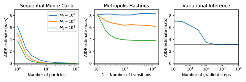
Figure 2: AIDE applies to SMC, variational, and MCMC algorithms. Left: AIDE estimates for SMC converge to zero, as expected. Right: AIDE estimates for variational inference converge to a nonzero asymptote that depends on the variational family. Middle: The symmetrized divergence between MH and the posterior converges to zero, but AIDE over-estimates the divergence in expectation. Although increasing the number of meta-inference runs Mtsubscript𝑀tM_{\mbox{t}} reduces the bias of AIDE, AIDE is not yet practical for measuring MH accuracy due to inaccurate meta-inference for MH.

2 Background

Consider a generative probabilistic model with latent variables X𝑋X and observed variables Y𝑌Y. We denote assignments to these variables by x𝒳𝑥𝒳x\in\mathcal{X} and y𝒴𝑦𝒴y\in\mathcal{Y}. Let p(x,y)𝑝𝑥𝑦p(x,y) denote the joint density of the generative model. The posterior density is p(x|y):=p(x,y)/p(y)assign𝑝conditional𝑥𝑦𝑝𝑥𝑦𝑝𝑦p(x|y):=p(x,y)/p(y) where p(y)=p(x,y)𝑑x𝑝𝑦𝑝𝑥𝑦differential-d𝑥p(y)=\int p(x,y)dx is the marginal likelihood, or ‘evidence’.

Sampling-based approximate inference strategies including Markov chain Monte Carlo (MCMC, [4, 5]), sequential Monte Carlo (SMC, [6]), annealed importance sampling (AIS, [7]) and importance sampling with resampling (SIR, [8, 9]), generate samples of the latent variables that are approximately distributed according to p(x|y)𝑝conditional𝑥𝑦p(x|y). Use of a sampling-based inference algorithm is often motivated by theoretical guarantees of exact convergence to the posterior in the limit of infinite computation (e.g. number of transitions in a Markov chain, number of importance samples in SIR). However, how well the sampling distribution approximates the posterior distribution for finite computation is typically difficult to analyze theoretically or estimate empirically with confidence.

Variational inference [10] explicitly minimizes the approximation error of the approximating distribution qθ(x)subscript𝑞𝜃𝑥q_{\theta}(x) over parameters θ𝜃\theta of a variational family. The error is usually quantified using the Kullback-Leibler (KL) divergence from the approximation qθ(x)subscript𝑞𝜃𝑥q_{\theta}(x) to the posterior p(x|y)𝑝conditional𝑥𝑦p(x|y), denoted DKL(qθ(x)p(x|y))D_{{\mbox{KL}}}(q_{\theta}(x)\;\|\;p(x|y)). Unlike sampling-based approaches, variational inference does not generally give exact results for infinite computation because the variational family does not include the posterior. Minimizing the KL divergence is performed by maximizing the ‘evidence lower bound’ (ELBO) =logp(y)DKL(qθ(x)p(x|y))\mathcal{L}=\log p(y)-D_{{\mbox{KL}}}(q_{\theta}(x)\;\|\;p(x|y)) over θ𝜃\theta. Since logp(y)𝑝𝑦\log p(y) is usually unknown, the actual error (the KL divergence) of a variational approximation is also unknown.

3 Estimating the symmetrized KL divergence between inference algorithms

This section defines our mathematical formalism for analyzing inference algorithms; shows how to represent SMC, MCMC, rejection sampling, and variational inference in this formalism; and introduces the Auxiliary Inference Divergence Estimator (AIDE), an algorithm for estimating the symmetrized KL divergence between two inference algorithms.

3.1 Generative inference models and meta-inference algorithms

We define an inference algorithm as a procedure that produces a single approximate posterior sample. Repeated runs of the algorithm give independent samples. For each inference algorithm, there is an ‘output density’ q(x)𝑞𝑥q(x) that represents the probability that the algorithm returns a given sample x𝑥x on any given run of the algorithm. Note that q(x)𝑞𝑥q(x) depends on the observations y𝑦y that define the inference problem, but we suppress that in the notation. The inference algorithm is accurate when q(x)p(x|y)𝑞𝑥𝑝conditional𝑥𝑦q(x)\approx p(x|y) for all x𝑥x. We denote a sample produced by running the algorithm by xq(x)similar-to𝑥𝑞𝑥x\sim q(x).

A naive simple Monte Carlo estimator of the KL divergence between the output distributions of two inference algorithms requires the output densities of both algorithms. However, it is typically intractable to compute the output densities of sampling-based inference algorithms like MCMC and SMC, because that would require marginalizing over all possible values that the random variables drawn during the algorithm could possibly take. A similar difficulty arises when computing the marginal likelihood p(y)𝑝𝑦p(y) of a generative probabilistic model p(x,y)𝑝𝑥𝑦p(x,y). This suggests that we treat the inference algorithm as a probabilistic model, estimate its output density using ideas from marginal likelihood estimation, and use these estimates in a Monte Carlo estimator of the divergence. We begin by making the analogy between an inference algorithm and a probabilistic model explicit:

Definition 3.1 (Generative inference model).

A generative inference model is a tuple (𝒰,𝒳,q)𝒰𝒳𝑞(\mathcal{U},\mathcal{X},q) where q(u,x)𝑞𝑢𝑥q(u,x) is a joint density defined on 𝒰×𝒳𝒰𝒳\mathcal{U}\times\mathcal{X}. A generative inference model models an inference algorithm if the output density of the inference algorithm is the marginal likelihood q(x)=q(u,x)𝑑u𝑞𝑥𝑞𝑢𝑥differential-d𝑢q(x)=\int q(u,x)du of the model for all x𝑥x. An element u𝒰𝑢𝒰u\in\mathcal{U} represents a complete assignment to the internal random variables within the inference algorithm, and is called a ‘trace’. The ability to simulate from q(u,x)𝑞𝑢𝑥q(u,x) is required, but the ability to compute the density q(u,x)𝑞𝑢𝑥q(u,x) is not. A simulation, denoted u,xq(u,x)similar-to𝑢𝑥𝑞𝑢𝑥u,x\sim q(u,x), may be obtained by running the inference algorithm and recording the resulting trace u𝑢u and output x𝑥x.111The trace data structure could in principle be obtained by writing the inference algorithm in a probabilistic programming language like Church [11], but the computational overhead would be high.

A generative inference model can be understood as a generative probabilistic model where the u𝑢u are the latent variables and the x𝑥x are the observations. Note that two different generative inference models may use different representations for the internal random variables of the same inference algorithm. In practice, constructing a generative inference model from an inference algorithm amounts to defining the set of internal random variables. For marginal likelihood estimation in a generative inference model, we use a ‘meta-inference’ algorithm:

Definition 3.2 (Meta-inference algorithm).

For a given generative inference model (𝒰,𝒳,q)𝒰𝒳𝑞(\mathcal{U},\mathcal{X},q), a meta-inference algorithm is a tuple (r,ξ)𝑟𝜉(r,\xi) where r(u;x)𝑟𝑢𝑥r(u;x) is a density on traces u𝒰𝑢𝒰u\in\mathcal{U} of the inference algorithm, indexed by outputs x𝒳𝑥𝒳x\in\mathcal{X} of the inference algorithm, and where ξ(u,x)𝜉𝑢𝑥\xi(u,x) is the following function of u𝑢u and x𝑥x for some Z>0𝑍0Z>0:

ξ(u,x):=Zq(u,x)r(u;x)assign𝜉𝑢𝑥𝑍𝑞𝑢𝑥𝑟𝑢𝑥\xi(u,x):=Z\frac{q(u,x)}{r(u;x)} (1)

We require the ability to sample ur(u;x)similar-to𝑢𝑟𝑢𝑥u\sim r(u;x) given a value for x𝑥x, and the ability to evaluate ξ(u,x)𝜉𝑢𝑥\xi(u,x) given u𝑢u and x𝑥x. We call a procedure for sampling from r(u;x)𝑟𝑢𝑥r(u;x) a ‘meta-inference sampler’. We do not require the ability to evaluate the density r(u;x)𝑟𝑢𝑥r(u;x).

A meta-inference algorithm is considered accurate for a given x𝑥x if r(u;x)q(u|x)𝑟𝑢𝑥𝑞conditional𝑢𝑥r(u;x)\approx q(u|x) for all u𝑢u. Conceptually, a meta-inference sampler tries to answer the question ‘how could my inference algorithm have produced this output x𝑥x?’ Note that if it is tractable to evaluate the marginal likelihood q(x)𝑞𝑥q(x) of the generative inference model up to a normalizing constant, then it is not necessary to represent internal random variables for the inference algorithm, and a generative inference model can define the trace as an empty token u=()𝑢u=() with 𝒰={()}𝒰\mathcal{U}=\{()\}. In this case, the meta-inference algorithm has r(u;x)=1𝑟𝑢𝑥1r(u;x)=1 for all x𝑥x and ξ(u,x)=Zq(x)𝜉𝑢𝑥𝑍𝑞𝑥\xi(u,x)=Zq(x).

3.2 Examples

We now show how to construct generative inference models and corresponding meta-inference algorithms for SMC, AIS, MCMC, SIR, rejection sampling, and variational inference. The meta-inference algorithms for AIS, MCMC, and SIR are derived as special cases of a generic SMC meta-inference algorithm.

Sequential Monte Carlo.

We consider a general class of SMC samplers introduced by Del Moral et al. [6], which can be used for approximate inference in both sequential state space and non-sequential models. We briefly summarize a slightly restricted variant of the algorithm here, and refer the reader to the supplement and Del Moral et al. [6] for full details. The SMC algorithm propagates P𝑃P weighted particles through T𝑇T steps, using proposal kernels ktsubscript𝑘𝑡k_{t} and multinomial resampling based on weight functions w1(x1)subscript𝑤1subscript𝑥1w_{1}(x_{1}) and wt(xt1,xt)subscript𝑤𝑡subscript𝑥𝑡1subscript𝑥𝑡w_{t}(x_{t-1},x_{t}) for t>1𝑡1t>1 that are defined in terms of ‘backwards kernels’ tsubscript𝑡\ell_{t} for t=2T𝑡2𝑇t=2\ldots T. Let xtisuperscriptsubscript𝑥𝑡𝑖x_{t}^{i}, wtisuperscriptsubscript𝑤𝑡𝑖w_{t}^{i} and Wtisuperscriptsubscript𝑊𝑡𝑖W_{t}^{i} denote the value, unnormalized weight, and normalized weight of particle i𝑖i at time t𝑡t, respectively. We define the output sample x𝑥x of SMC as a single draw from the particle approximation at the final time step, which is obtained by sampling a particle index ITCategorical(WT1:P)similar-tosubscript𝐼𝑇Categoricalsuperscriptsubscript𝑊𝑇:1𝑃I_{T}\sim\mbox{Categorical}(W_{T}^{1:P}) where WT1:Psuperscriptsubscript𝑊𝑇:1𝑃W_{T}^{1:P} denotes the vector of weights (WT1,,WTP)superscriptsubscript𝑊𝑇1superscriptsubscript𝑊𝑇𝑃(W_{T}^{1},\ldots,W_{T}^{P}), and then setting xxTIT𝑥subscriptsuperscript𝑥subscript𝐼𝑇𝑇x\leftarrow x^{I_{T}}_{T}. The generative inference model uses traces of the form u=(𝐱,𝐚,IT)𝑢𝐱𝐚subscript𝐼𝑇u=(\mathbf{x},\mathbf{a},I_{T}), where 𝐱𝐱\mathbf{x} contains the values of all particles at all time steps and where 𝐚𝐚\mathbf{a} (for ‘ancestor’) contains the index ati{1P}superscriptsubscript𝑎𝑡𝑖1𝑃a_{t}^{i}\in\{1\ldots P\} of the parent of particle xt+1isuperscriptsubscript𝑥𝑡1𝑖x_{t+1}^{i} for each particle i𝑖i and each time step t=1T1𝑡1𝑇1t=1\ldots T-1. Algorithm 1 defines a canonical meta-inference sampler for this generative inference model that takes as input a latent sample x𝑥x and generates an SMC trace ur(u;x)similar-to𝑢𝑟𝑢𝑥u\sim r(u;x) as output. The meta-inference sampler first generates an ancestral trajectory of particles (x1I1,x2I2,,xTIT)superscriptsubscript𝑥1subscript𝐼1superscriptsubscript𝑥2subscript𝐼2superscriptsubscript𝑥𝑇subscript𝐼𝑇(x_{1}^{I_{1}},x_{2}^{I_{2}},\ldots,x_{T}^{I_{T}}) that terminates in the output sample x𝑥x, by sampling sequentially from the backward kernels tsubscript𝑡\ell_{t}, starting from xTIT=xsuperscriptsubscript𝑥𝑇subscript𝐼𝑇𝑥x_{T}^{I_{T}}=x. Next, it runs a conditional SMC update [2] conditioned on the ancestral trajectory. For this choice of r(u;x)𝑟𝑢𝑥r(u;x) and for Z=1𝑍1Z=1, the function ξ(u,x)𝜉𝑢𝑥\xi(u,x) is closely related to the marginal likelihood estimate p(y)^^𝑝𝑦\widehat{p(y)} produced by the SMC scheme:222AIDE also applies to approximate inference algorithms for undirected probabilistic models; the marginal likelihood estimate is replaced with the estimate of the partition function. ξ(u,x)=p(x,y)/p(y)^𝜉𝑢𝑥𝑝𝑥𝑦^𝑝𝑦\xi(u,x)=p(x,y)/\widehat{p(y)}. See supplement for derivation.

Algorithm 1 Generalized conditional SMC (a canonical meta-inference sampler for SMC)
Latent sample x𝑥x, SMC parameters
ITUniform(1P)similar-tosubscript𝐼𝑇Uniform1𝑃I_{T}\sim\mbox{Uniform}(1\ldots P)
xTITxsuperscriptsubscript𝑥𝑇subscript𝐼𝑇𝑥x_{T}^{I_{T}}\leftarrow x
for tT11𝑡𝑇11t\leftarrow T-1\ldots 1 do
     ItUniform(1P)similar-tosubscript𝐼𝑡Uniform1𝑃I_{t}\sim\mbox{Uniform}(1\ldots P)
     \triangleright Sample from backward kernel
     xtItt+1(;xt+1It+1)similar-tosuperscriptsubscript𝑥𝑡subscript𝐼𝑡subscript𝑡1superscriptsubscript𝑥𝑡1subscript𝐼𝑡1x_{t}^{I_{t}}\sim\ell_{t+1}(\cdot;x_{t+1}^{I_{t+1}})
for i1P𝑖1𝑃i\leftarrow 1\ldots P do
     if iI1𝑖subscript𝐼1i\neq I_{1} then x1ik1()similar-tosubscriptsuperscript𝑥𝑖1subscript𝑘1x^{i}_{1}\sim k_{1}(\cdot)
     w1iw1(x1i)subscriptsuperscript𝑤𝑖1subscript𝑤1subscriptsuperscript𝑥𝑖1w^{i}_{1}\leftarrow w_{1}(x^{i}_{1})
for t2T𝑡2𝑇t\leftarrow 2\ldots T do
     Wt11:Pwt11:P/(i=1Pwt1i)superscriptsubscript𝑊𝑡1:1𝑃superscriptsubscript𝑤𝑡1:1𝑃superscriptsubscript𝑖1𝑃superscriptsubscript𝑤𝑡1𝑖W_{t-1}^{1:P}\leftarrow w_{t-1}^{1:P}/(\sum_{i=1}^{P}w_{t-1}^{i})
     for i1P𝑖1𝑃i\leftarrow 1\ldots P do
         if i=It𝑖subscript𝐼𝑡i=I_{t} then at1iIt1superscriptsubscript𝑎𝑡1𝑖subscript𝐼𝑡1a_{t-1}^{i}\leftarrow I_{t-1}
         else
              at1iCategorical(Wt11:P)similar-tosuperscriptsubscript𝑎𝑡1𝑖Categoricalsuperscriptsubscript𝑊𝑡1:1𝑃a_{t-1}^{i}\sim\mbox{Categorical}(W_{t-1}^{1:P})
              xtikt(;xt1at1i)similar-tosubscriptsuperscript𝑥𝑖𝑡subscript𝑘𝑡superscriptsubscript𝑥𝑡1superscriptsubscript𝑎𝑡1𝑖x^{i}_{t}\sim k_{t}(\cdot;x_{t-1}^{a_{t-1}^{i}})          
         wtiwt(xt1at1i,xti)superscriptsubscript𝑤𝑡𝑖subscript𝑤𝑡superscriptsubscript𝑥𝑡1superscriptsubscript𝑎𝑡1𝑖superscriptsubscript𝑥𝑡𝑖w_{t}^{i}\leftarrow w_{t}(x_{t-1}^{a_{t-1}^{i}},x_{t}^{i})      
u(𝐱,𝐚,IT)𝑢𝐱𝐚subscript𝐼𝑇u\leftarrow(\mathbf{x},\mathbf{a},I_{T})\quad \triangleright Return an SMC trace
return u𝑢u
x11superscriptsubscript𝑥11x_{1}^{1}x12superscriptsubscript𝑥12x_{1}^{2}x13superscriptsubscript𝑥13x_{1}^{3}x14superscriptsubscript𝑥14x_{1}^{4}x21superscriptsubscript𝑥21x_{2}^{1}x22superscriptsubscript𝑥22x_{2}^{2}x23superscriptsubscript𝑥23x_{2}^{3}x24superscriptsubscript𝑥24x_{2}^{4}x31superscriptsubscript𝑥31x_{3}^{1}x32superscriptsubscript𝑥32x_{3}^{2}x33superscriptsubscript𝑥33x_{3}^{3}x34superscriptsubscript𝑥34x_{3}^{4}x𝑥xLatent sample(input to meta-inference sampler)2subscript2\ell_{2}3subscript3\ell_{3}δ𝛿\deltaI1=1subscript𝐼11I_{1}=1I2=3subscript𝐼23I_{2}=3I3=2subscript𝐼32I_{3}=2T=3𝑇3T=3xtisuperscriptsubscript𝑥𝑡𝑖x_{t}^{i}Member of ancestraltrajectory
Annealed importance sampling.

When a single particle is used (P=1𝑃1P=1), and when each forward kernel ktsubscript𝑘𝑡k_{t} satisfies detailed balance for some intermediate density, the SMC algorithm simplifies to annealed importance sampling (AIS, [7]), and the canonical SMC meta-inference inference (Algorithm 1) consists of running the forward kernels in reverse order, as in the reverse annealing algorithm of Grosse et al. [3, 12]. The canonical meta-inference algorithm is accurate (r(u;x)q(u;x)𝑟𝑢𝑥𝑞𝑢𝑥r(u;x)\approx q(u;x)) if the AIS Markov chain is kept close to equilibrium at all times. This is achieved if the intermediate densities form a sufficiently fine-grained sequence. See supplement for analysis.

Markov chain Monte Carlo.

We define each run of an MCMC algorithm as producing a single output sample x𝑥x that is the iterate of the Markov chain produced after a predetermined number of burn-in steps has passed. We also assume that each MCMC transition operator satisfies detailed balance with respect to the posterior p(x|y)𝑝conditional𝑥𝑦p(x|y). Then, this is formally a special case of AIS. However, unless the Markov chain was initialized near the posterior p(x|y)𝑝conditional𝑥𝑦p(x|y), the chain will be far from equilibrium during the burn-in period, and the AIS meta-inference algorithm will be inaccurate.

Importance sampling with resampling.

Importance sampling with resampling, or SIR [8] can be seen as a special case of SMC if we set the number of steps to one (T=1𝑇1T=1). The trace of the SIR algorithm is then the set of particles x1isuperscriptsubscript𝑥1𝑖x_{1}^{i} for i{1,,P}𝑖1𝑃i\in\{1,\ldots,P\} and output particle index I1subscript𝐼1I_{1}. Given output sample x𝑥x, the canonical SMC meta-inference sampler then simply samples I1Uniform(1P)similar-tosubscript𝐼1Uniform1𝑃I_{1}\sim\mbox{Uniform}(1\ldots P), sets x1I1xsuperscriptsubscript𝑥1subscript𝐼1𝑥x_{1}^{I_{1}}\leftarrow x, and samples the other P1𝑃1P-1 particles from the importance distribution k1(x)subscript𝑘1𝑥k_{1}(x).

Rejection sampling.

To model a rejection sampler for a posterior distribution p(x|y)𝑝conditional𝑥𝑦p(x|y), we assume it is tractable to evaluate the unnormalized posterior density p(x,y)𝑝𝑥𝑦p(x,y). We define 𝒰={()}𝒰\mathcal{U}=\{()\} as described in Section 3.1. For meta-inference, we define Z=p(y)𝑍𝑝𝑦Z=p(y) so that ξ(u,x)=p(y)p(x|y)=p(x,y)𝜉𝑢𝑥𝑝𝑦𝑝conditional𝑥𝑦𝑝𝑥𝑦\xi(u,x)=p(y)p(x|y)=p(x,y). It is not necessary to represent the internal random variables of the rejection sampler.

Variational inference.

We suppose a variational approximation qθ(x)subscript𝑞𝜃𝑥q_{\theta}(x) has been computed through optimization over the variational parameters θ𝜃\theta. We assume that it is possible to sample from the variational approximation, and evaluate its normalized density. Then, we use 𝒰={()}𝒰\mathcal{U}=\{()\} and Z=1𝑍1Z=1 and ξ(u,x)=qθ(x)𝜉𝑢𝑥subscript𝑞𝜃𝑥\xi(u,x)=q_{\theta}(x). Note that this formulation also applies to amortized variational inference algorithms, which reuse the parameters θ𝜃\theta for inference across different observation contexts y𝑦y.

3.3 The auxiliary inference divergence estimator

Consider a probabilistic model p(x,y)𝑝𝑥𝑦p(x,y), a set of observations y𝑦y, and two inference algorithms that approximate p(x|y)𝑝conditional𝑥𝑦p(x|y). One of the two inference algorithms is considered the ‘gold-standard’, and has a generative inference model (𝒰,𝒳,qg)𝒰𝒳subscript𝑞g(\mathcal{U},\mathcal{X},q_{\mbox{g}}) and a meta-inference algorithm (rg,ξg)subscript𝑟gsubscript𝜉g(r_{\mbox{g}},\xi_{\mbox{g}}). The second algorithm is considered the ‘target’ algorithm, with a generative inference model (𝒱,𝒳,qt)𝒱𝒳subscript𝑞t(\mathcal{V},\mathcal{X},q_{\mbox{t}}) (we denote a trace of the target algorithm by v𝒱𝑣𝒱v\in\mathcal{V}), and a meta-inference algorithm (rt,ξt)subscript𝑟tsubscript𝜉t(r_{\mbox{t}},\xi_{\mbox{t}}). This section shows how to estimate an upper bound on the symmetrized KL divergence between qg(x)subscript𝑞g𝑥q_{\mbox{g}}(x) and qt(x)subscript𝑞t𝑥q_{\mbox{t}}(x), which is:

DKL(qg(x)qt(x))+DKL(qt(x)qg(x))=𝔼xqg(x)[logqg(x)qt(x)]+𝔼xqt(x)[logqt(x)qg(x)]subscript𝐷KLconditionalsubscript𝑞g𝑥subscript𝑞t𝑥subscript𝐷KLconditionalsubscript𝑞t𝑥subscript𝑞g𝑥subscript𝔼similar-to𝑥subscript𝑞g𝑥delimited-[]subscript𝑞g𝑥subscript𝑞t𝑥subscript𝔼similar-to𝑥subscript𝑞t𝑥delimited-[]subscript𝑞t𝑥subscript𝑞g𝑥D_{{\mbox{KL}}}(q_{\mbox{g}}(x)\;\|\;q_{\mbox{t}}(x))+D_{{\mbox{KL}}}(q_{\mbox{t}}(x)\;\|\;q_{\mbox{g}}(x))=\mathbb{E}_{x\sim q_{\mbox{g}}(x)}\left[\log\frac{q_{\mbox{g}}(x)}{q_{\mbox{t}}(x)}\right]+\mathbb{E}_{x\sim q_{\mbox{t}}(x)}\left[\log\frac{q_{\mbox{t}}(x)}{q_{\mbox{g}}(x)}\right] (2)

We take a Monte Carlo approach. Simple Monte Carlo applied to the Equation (2) requires that qg(x)subscript𝑞g𝑥q_{\mbox{g}}(x) and qt(x)subscript𝑞t𝑥q_{\mbox{t}}(x) can be evaluated, which would prevent the estimator from being used when either inference algorithm is sampling-based. Algorithm 2 gives the Auxiliary Inference Divergence Estimator (AIDE), an estimator of the symmetrized KL divergence that only requires evaluation of ξg(u,x)subscript𝜉g𝑢𝑥\xi_{\mbox{g}}(u,x) and ξt(v,x)subscript𝜉t𝑣𝑥\xi_{\mbox{t}}(v,x) and not qg(x)subscript𝑞g𝑥q_{\mbox{g}}(x) or qt(x)subscript𝑞t𝑥q_{\mbox{t}}(x), permitting its use with sampling-based inference algorithms.

Algorithm 2 Auxiliary Inference Divergence Estimator (AIDE)
Gold-standard inference model and meta-inference algorithm (𝒰,𝒳,qg)𝒰𝒳subscript𝑞g(\mathcal{U},\mathcal{X},q_{\mbox{g}}) and (rg,ξg)subscript𝑟gsubscript𝜉g(r_{\mbox{g}},\xi_{\mbox{g}})
Target inference model and meta-inference algorithm (𝒱,𝒳,qt)𝒱𝒳subscript𝑞t(\mathcal{V},\mathcal{X},q_{\mbox{t}}) and (rt,ξt)subscript𝑟tsubscript𝜉t(r_{\mbox{t}},\xi_{\mbox{t}})
Number of runs of gold-standard algorithm Ngsubscript𝑁gN_{\mbox{g}}
Number of runs of meta-inference sampler for gold-standard Mgsubscript𝑀gM_{\mbox{g}}
Number of runs of target algorithm Ntsubscript𝑁tN_{\mbox{t}}
Number of runs of meta-inference sampler for target Mtsubscript𝑀tM_{\mbox{t}}
for n1Ng𝑛1subscript𝑁gn\leftarrow 1\ldots N_{\mbox{g}} do
     un,1,xnqg(u,x)similar-tosubscript𝑢𝑛1subscript𝑥𝑛subscript𝑞g𝑢𝑥u_{n,1},x_{n}\sim q_{\mbox{g}}(u,x)     \triangleright Run gold-standard algorithm, record trace un,1subscript𝑢𝑛1u_{n,1} and output xnsubscript𝑥𝑛x_{n}
     for m2Mg𝑚2subscript𝑀gm\leftarrow 2\ldots M_{\mbox{g}} do
         un,mrg(u;xn)similar-tosubscript𝑢𝑛𝑚subscript𝑟g𝑢subscript𝑥𝑛u_{n,m}\sim r_{\mbox{g}}(u;x_{n})\triangleright Run meta-inference sampler for gold-standard algorithm, on input xnsubscript𝑥𝑛x_{n}      
     for m1Mt𝑚1subscript𝑀tm\leftarrow 1\ldots M_{\mbox{t}} do
         vn,mrt(v;xn)similar-tosubscript𝑣𝑛𝑚subscript𝑟t𝑣subscript𝑥𝑛v_{n,m}\sim r_{\mbox{t}}(v;x_{n})   \triangleright Run meta-inference sampler for target algorithm, on input xnsubscript𝑥𝑛x_{n}      
for n1Nt𝑛1subscript𝑁tn\leftarrow 1\ldots N_{\mbox{t}} do
     vn,1,xnqt(v,x)similar-tosuperscriptsubscript𝑣𝑛1superscriptsubscript𝑥𝑛subscript𝑞t𝑣𝑥v_{n,1}^{\prime},x_{n}^{\prime}\sim q_{\mbox{t}}(v,x)      \triangleright Run target algorithm, record trace vn,1superscriptsubscript𝑣𝑛1v_{n,1}^{\prime} and output xnsuperscriptsubscript𝑥𝑛x_{n}^{\prime}
     for m2Mt𝑚2subscript𝑀tm\leftarrow 2\ldots M_{\mbox{t}} do
         vn,mrt(v;xn)similar-tosuperscriptsubscript𝑣𝑛𝑚subscript𝑟t𝑣superscriptsubscript𝑥𝑛v_{n,m}^{\prime}\sim r_{\mbox{t}}(v;x_{n}^{\prime})   \triangleright Run meta-inference sampler for target algorithm, on input xnsuperscriptsubscript𝑥𝑛x_{n}^{\prime}      
     for m1Mg𝑚1subscript𝑀gm\leftarrow 1\ldots M_{\mbox{g}} do
         un,mrg(u;xn)similar-tosuperscriptsubscript𝑢𝑛𝑚subscript𝑟g𝑢superscriptsubscript𝑥𝑛u_{n,m}^{\prime}\sim r_{\mbox{g}}(u;x_{n}^{\prime})\triangleright Run meta-inference sampler for gold-standard algorithm, on input xnsuperscriptsubscript𝑥𝑛x_{n}^{\prime}      
D^1Ngn=1Nglog(1Mgm=1Mgξg(un,m,xn)1Mtm=1Mtξt(vn,m,xn))+1Ntn=1Ntlog(1Mtm=1Mtξt(vn,m,xn)1Mgm=1Mgξg(un,m,xn))^𝐷1subscript𝑁gsuperscriptsubscript𝑛1subscript𝑁g1subscript𝑀gsuperscriptsubscript𝑚1subscript𝑀gsubscript𝜉gsubscript𝑢𝑛𝑚subscript𝑥𝑛1subscript𝑀tsuperscriptsubscript𝑚1subscript𝑀tsubscript𝜉tsubscript𝑣𝑛𝑚subscript𝑥𝑛1subscript𝑁tsuperscriptsubscript𝑛1subscript𝑁t1subscript𝑀tsuperscriptsubscript𝑚1subscript𝑀tsubscript𝜉tsuperscriptsubscript𝑣𝑛𝑚superscriptsubscript𝑥𝑛1subscript𝑀gsuperscriptsubscript𝑚1subscript𝑀gsubscript𝜉gsuperscriptsubscript𝑢𝑛𝑚superscriptsubscript𝑥𝑛\hat{D}\leftarrow\displaystyle\frac{1}{N_{\mbox{g}}}\sum_{n=1}^{N_{\mbox{g}}}\log\left(\frac{\frac{1}{M_{\mbox{g}}}\sum_{m=1}^{M_{\mbox{g}}}\xi_{\mbox{g}}(u_{n,m},x_{n})}{\frac{1}{M_{\mbox{t}}}\sum_{m=1}^{M_{\mbox{t}}}\xi_{\mbox{t}}(v_{n,m},x_{n})}\right)+\frac{1}{N_{\mbox{t}}}\sum_{n=1}^{N_{\mbox{t}}}\log\left(\frac{\frac{1}{M_{\mbox{t}}}\sum_{m=1}^{M_{\mbox{t}}}\xi_{\mbox{t}}(v_{n,m}^{\prime},x_{n}^{\prime})}{\frac{1}{M_{\mbox{g}}}\sum_{m=1}^{M_{\mbox{g}}}\xi_{\mbox{g}}(u_{n,m}^{\prime},x_{n}^{\prime})}\right)
return D^^𝐷\hat{D} \triangleright D^^𝐷\hat{D} is an estimate of DKL(qg(x)||qt(x))+DKL(qt(x)||qg(x))D_{\mbox{KL}}(q_{\mbox{g}}(x)||q_{\mbox{t}}(x))+D_{\mbox{KL}}(q_{\mbox{t}}(x)||q_{\mbox{g}}(x))

The generic AIDE algorithm above is defined in terms of abstract generative inference models and meta-inference algorithms. For concreteness, the supplement contains the AIDE algorithm specialized to the case when the gold-standard is AIS and the target is a variational approximation.

Theorem 1.

The estimate D^^𝐷\hat{D} produced by AIDE is an upper bound on the symmetrized KL divergence in expectation, and the expectation is nonincreasing in AIDE parameters Mgsubscript𝑀gM_{\mbox{g}} and Mtsubscript𝑀tM_{\mbox{t}}.

See supplement for proof. Briefly, AIDE estimates an upper bound on the symmetrized divergence in expectation because it uses unbiased estimates of qt(xn)subscript𝑞tsubscript𝑥𝑛q_{\mbox{t}}(x_{n}) and qg(xn)1subscript𝑞gsuperscriptsubscript𝑥𝑛1q_{\mbox{g}}(x_{n})^{-1} for xnqg(x)similar-tosubscript𝑥𝑛subscript𝑞g𝑥x_{n}\sim q_{\mbox{g}}(x), and unbiased estimates of qg(xn)subscript𝑞gsuperscriptsubscript𝑥𝑛q_{\mbox{g}}(x_{n}^{\prime}) and qt(xn)1subscript𝑞tsuperscriptsuperscriptsubscript𝑥𝑛1q_{\mbox{t}}(x_{n}^{\prime})^{-1} for xnqt(x)similar-tosuperscriptsubscript𝑥𝑛subscript𝑞t𝑥x_{n}^{\prime}\sim q_{\mbox{t}}(x). For Mg=1subscript𝑀g1M_{\mbox{g}}=1 and Mt=1subscript𝑀t1M_{\mbox{t}}=1, AIDE over-estimates the true symmetrized divergence by:

𝔼[D^](DKL(qg(x)qt(x))+DKL(qt(x)qg(x)))=(𝔼xqg(x)[DKL(qg(u|x)rg(u;x))+DKL(rt(v;x)qt(v|x))]+𝔼xqt(x)[DKL(qt(v|x)rt(v;x))+DKL(rg(u;x)qg(u|x))])Bias of AIDEfor Mg=Mt=1\begin{array}[]{ll}&\mathbb{E}[\hat{D}]-(D_{{\mbox{KL}}}(q_{\mbox{g}}(x)\;\|\;q_{\mbox{t}}(x))+D_{{\mbox{KL}}}(q_{\mbox{t}}(x)\;\|\;q_{\mbox{g}}(x)))=\\[5.0pt] &\left(\begin{array}[]{ll}&\mathbb{E}_{x\sim q_{\mbox{g}}(x)}\left[D_{{\mbox{KL}}}(q_{\mbox{g}}(u|x)\;\|\;r_{\mbox{g}}(u;x))+D_{{\mbox{KL}}}(r_{\mbox{t}}(v;x)\;\|\;q_{\mbox{t}}(v|x))\right]\\ +&\mathbb{E}_{x\sim q_{\mbox{t}}(x)}\left[D_{{\mbox{KL}}}(q_{\mbox{t}}(v|x)\;\|\;r_{\mbox{t}}(v;x))+D_{{\mbox{KL}}}(r_{\mbox{g}}(u;x)\;\|\;q_{\mbox{g}}(u|x))\right]\end{array}\right)\end{array}\begin{array}[]{c}\text{Bias of AIDE}\\ \text{for }{\scriptstyle M_{\mbox{g}}=M_{\mbox{t}}=1}\end{array} (3)

Note that this expression involves KL divergences between the meta-inference sampling densities (rg(u;x)subscript𝑟g𝑢𝑥r_{\mbox{g}}(u;x) and rt(v;x)subscript𝑟t𝑣𝑥r_{\mbox{t}}(v;x)) and the posteriors in their respective generative inference models (qg(u|x)subscript𝑞gconditional𝑢𝑥q_{\mbox{g}}(u|x) and qt(v|x)subscript𝑞tconditional𝑣𝑥q_{\mbox{t}}(v|x)). Therefore, the approximation error of meta-inference determines the bias of AIDE. When both meta-inference algorithms are exact (rg(u;x)=qg(u|x)subscript𝑟g𝑢𝑥subscript𝑞gconditional𝑢𝑥r_{\mbox{g}}(u;x)=q_{\mbox{g}}(u|x) for all u𝑢u and x𝑥x and rt(v;x)=qt(v|x)subscript𝑟t𝑣𝑥subscript𝑞tconditional𝑣𝑥r_{\mbox{t}}(v;x)=q_{\mbox{t}}(v|x) for all v𝑣v and x𝑥x), AIDE is unbiased. As Mgsubscript𝑀gM_{\mbox{g}} or Mtsubscript𝑀tM_{\mbox{t}} are increased, the bias decreases (see Figure 2 and Figure 4 for examples). If the generative inference model for one of the algorithms does not use a trace (i.e. 𝒰={()}𝒰\mathcal{U}=\{()\} or 𝒱={()}𝒱\mathcal{V}=\{()\}), then that algorithm does not contribute a KL divergence term to the bias of Equation (3). The analysis of AIDE is equivalent to that of Grosse et al. [12] when the target algorithm is AIS and Mt=Mg=1subscript𝑀tsubscript𝑀g1M_{\mbox{t}}=M_{\mbox{g}}=1 and the gold-standard inference algorithm is a rejection sampler.

4 Related Work

Diagnosing the convergence of approximate inference is a long-standing problem. Most existing work is either tailored to specific inference algorithms [13], designed to detect lack of exact convergence [1], or both. Estimators of the non-asymptotic approximation error of general approximate inference algorithms have received less attention. Gorham and Mackey [14] propose an approach that applies to arbitrary sampling algorithms but relies on special properties of the posterior density such as log-concavity. Our approach does not rely on special properties of the posterior distribution.

Our work is most closely related to Bounding Divergences with REverse Annealing (BREAD, [12]) which also estimates upper bounds on the symmetric KL divergence between the output distribution of a sampling algorithm and the posterior distribution. AIDE differs from BREAD in two ways: First, whereas BREAD handles single-particle SMC samplers and annealed importance sampling (AIS), AIDE handles a substantially broader family of inference algorithms including SMC samplers with both resampling and rejuvenation steps, AIS, variational inference, and rejection samplers. Second, BREAD estimates divergences between the target algorithm’s sampling distribution and the posterior distribution, but the exact posterior samples necessary for BREAD’s theoretical properties are only readily available when the observations y𝑦y that define the inference problem are simulated from the generative model. Instead, AIDE estimates divergences against an exact or approximate gold-standard sampler on real (non-simulated) inference problems. Unlike BREAD, AIDE can be used to evaluate inference in both generative and undirected models.

AIDE estimates the error of sampling-based inference using a mathematical framework with roots in variational inference. Several recent works have treated sampling-based inference algorithms as variational approximations. The Monte Carlo Objective (MCO) formalism of Maddison et al. [15] is closely related to our formalism of generative inference models and meta-inference algorithms—indeed a generative inference model and a meta-inference algorithm with Z=1𝑍1Z=1 give an MCO defined by: (y,p)=𝔼u,xq(u,x)[log(p(x,y)/ξ(u,x))]𝑦𝑝subscript𝔼similar-to𝑢𝑥𝑞𝑢𝑥delimited-[]𝑝𝑥𝑦𝜉𝑢𝑥\mathcal{L}(y,p)=\mathbb{E}_{u,x\sim q(u,x)}[\log(p(x,y)/\xi(u,x))], where y𝑦y denotes observed data. In independent and concurrent work to our own, Naesseth et al. [16], Maddison et al. [15] and Le et al. [17] treat SMC as a variational approximation using constructions similar to ours. In earlier work, Salimans et al. [18] recognized that MCMC samplers can be treated as variational approximations. However, these works are concerned with optimization of variational objective functions instead of estimation of KL divergences, and do not involve generating a trace of a sampler from its output.
Refer to caption
Refer to caption
Refer to caption
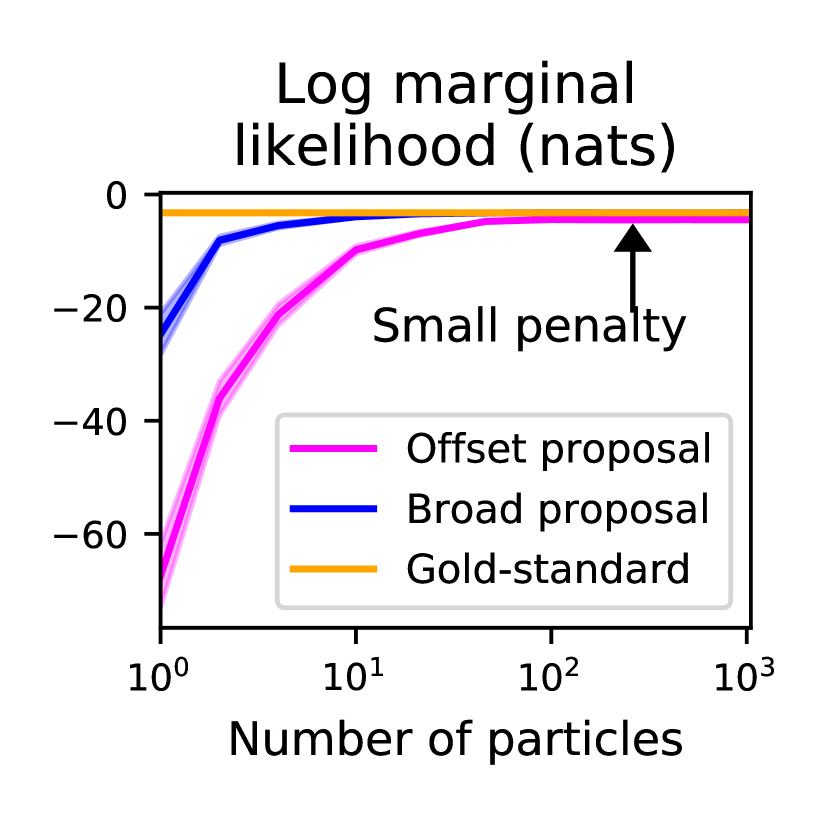
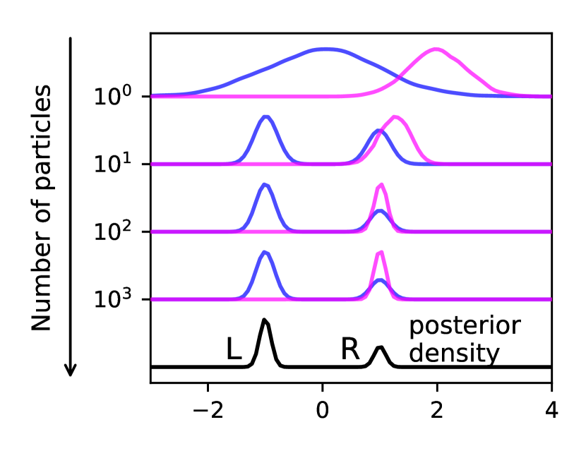
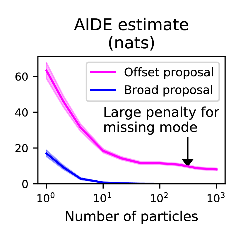
Figure 3: AIDE detects when an inference algorithm misses a posterior mode. Left: A bimodal posterior density, with kernel estimates of the output densities of importance sampling with resampling (SIR) using two proposals. The ‘broad’ proposal (blue) covers both modes, and the ‘offset’ proposal (pink) misses the ‘L’ mode. Middle: AIDE detects the missing mode in offset-proposal SIR. Right: Log marginal likelihood estimates suggest that the offset-proposal SIR is nearly converged.

5 Experiments

5.1 Comparing the bias of AIDE for different types of inference algorithms

We used a Bayesian linear regression inference problem where exact posterior sampling is tractable to characterize the bias of AIDE when applied to three different types of target inference algorithms: sequential Monte Carlo (SMC), Metropolis-Hastings (MH), and variational inference. For the gold-standard algorithm we used a posterior sampler with a tractable output density qg(x)subscript𝑞g𝑥q_{\mbox{g}}(x), which does not introduce bias into AIDE, so that the AIDE’s bias could be completely attributed to the approximation error of meta-inference for each target algorithm. Figure 2 shows the results. The bias of AIDE is acceptable for SMC, and AIDE is unbiased for variational inference, but better meta-inference algorithms for MCMC are needed to make AIDE practical for estimating the accuracy of MH.

5.2 Evaluating approximate inference in a Hidden Markov model

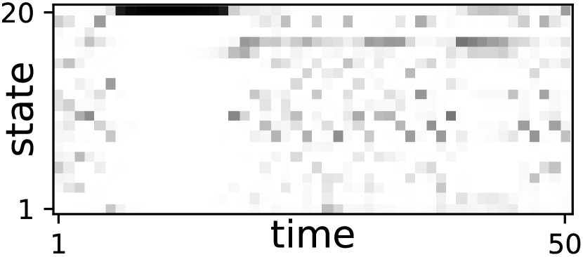
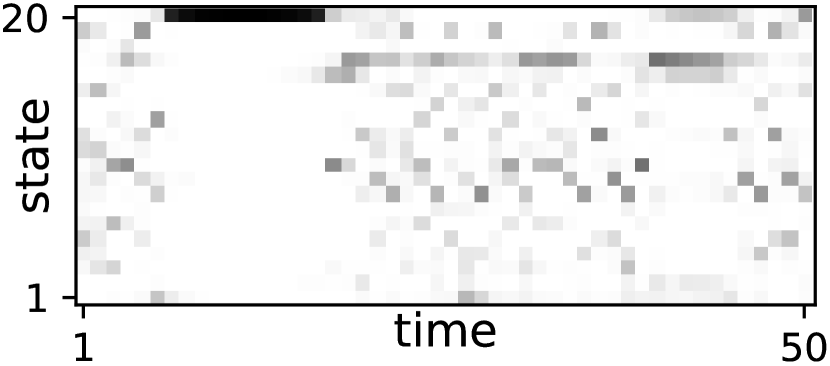
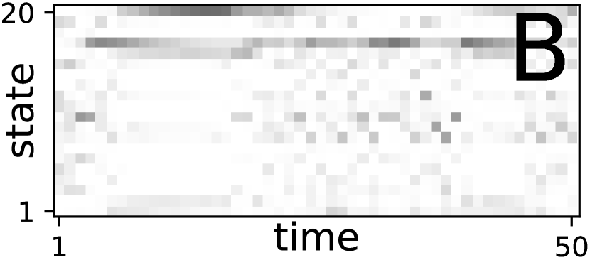
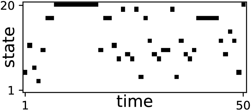
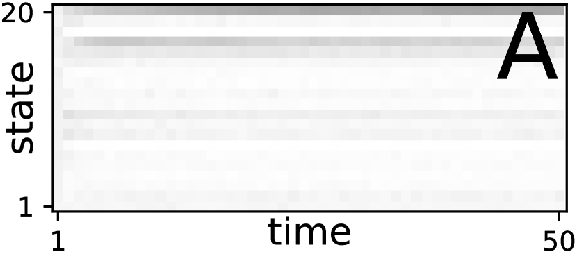
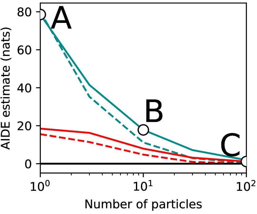
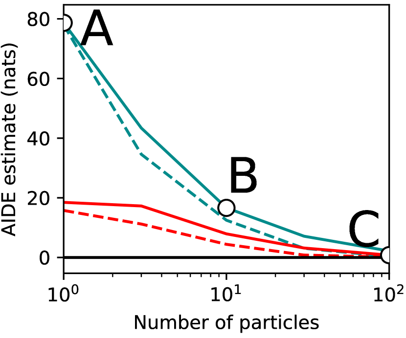
We applied AIDE to measure the approximation error of SMC algorithms for posterior inference in a Hidden Markov model (HMM). Because exact posterior inference in this HMM is tractable via dynamic programming, we used this opportunity to compare AIDE estimates obtained using the exact posterior as the gold-standard with AIDE estimates obtained using a ‘best-in-class’ SMC algorithm as the gold-standard. Figure 4 shows the results, which indicate AIDE estimates using an approximate gold-standard algorithm can be nearly identical to AIDE estimates obtained with an exact posterior gold-standard.
Refer to caption

Ground truth states

Refer to caption

Posterior marginals

Refer to caption

SMC optimal proposal

1000 particles

(SMC gold standard)

Target algorithms
  Refer to caption

SMC prior proposal

1 particle

Refer to caption

SMC prior proposal

10 particles

Refer to caption

SMC optimal proposal

100 particles

Measuring accuracy

of target algorithms using

posterior as gold-standard
Refer to caption

Measuring accuracy

of target algorithms using

SMC gold-standard
Refer to caption
Refer to caption
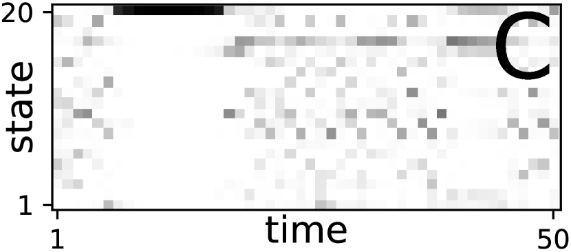
Figure 4: Comparing use of an exact posterior as the gold-standard and a ‘best-in-class’ approximate algorithm as the gold-standard, when measuring accuracy of target inference algorithms with AIDE. We consider inference in an HMM, so that exact posterior sampling is tractable using dynamic programming. Left: Ground truth latent states, posterior marginals, and marginals of the the output of a gold-standard and three target SMC algorithms (A,B,C) for a particular observation sequence. Right: AIDE estimates using the exact gold-standard and using the SMC gold-standard are nearly identical. The estimated divergence bounds decrease as the number of particles in the target sampler increases. The optimal proposal outperforms the prior proposal. Increasing Mtsubscript𝑀tM_{\mbox{t}} tightens the estimated divergence bounds. We used Mg=1subscript𝑀g1M_{\mbox{g}}=1.
Refer to caption
Refer to caption
Refer to caption
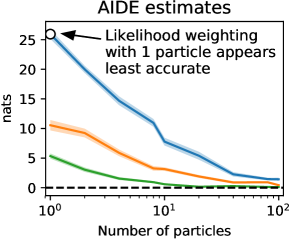
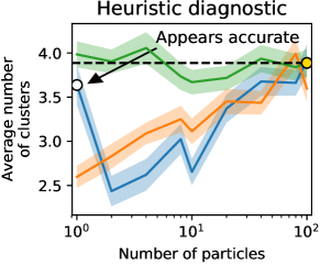
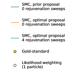
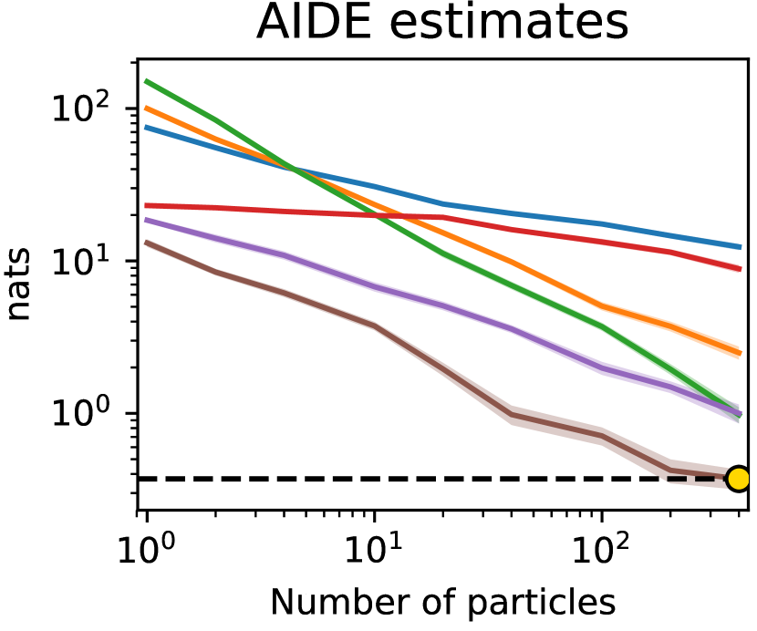
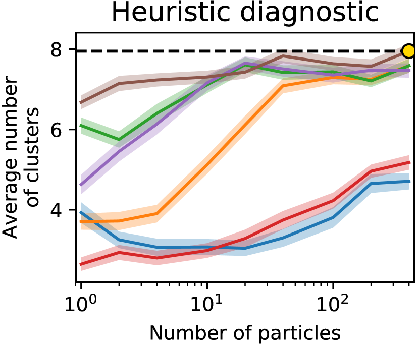
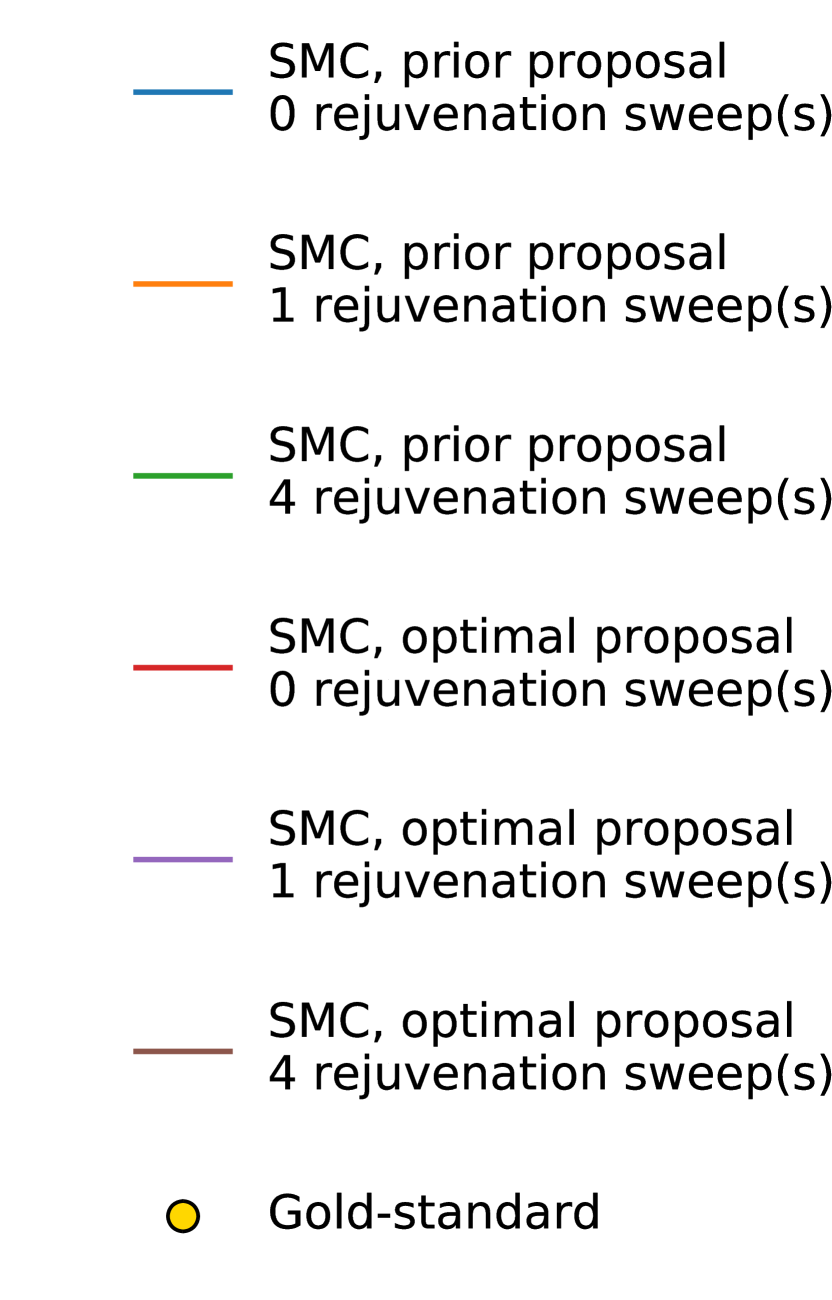
Figure 5: Contrasting AIDE against a heuristic convergence diagnostic for evaluating the accuracy of approximate inference in a Dirichlet process mixture model (DPMM). The heuristic compares the expected number of clusters under the target algorithm to the expectation under the gold-standard algorithm [19]. White circles identify single-particle likelihood-weighting, which samples from the prior. AIDE clearly indicates that single-particle likelihood-weighting is inaccurate, but the heuristic suggests it is accurate. Probe functions like the expected number of clusters can be error prone measures of convergence because they only track convergence along a specific projection of the distribution. In contrast, AIDE estimates a joint KL divergence. Shaded areas in both plots show the standard error. The amount of target inference computation used is the same for the two techniques, although AIDE performs a gold-standard meta-inference run for each target inference run.

5.3 Comparing AIDE to alternative inference evaluation techniques

A key feature of AIDE is that it applies to different types of inference algorithms. We compared AIDE to two existing techniques for evaluating the accuracy of inference algorithms that share this feature: (1) comparing log marginal likelihood (LML) estimates made by a target algorithm against LML estimates made by a gold-standard algorithm, and (2) comparing the expectation of a probe function under the approximating distribution to the same expectation under the gold-standard distribution [19]. Figure 3 shows a comparison of AIDE to LML, on a inference problem where the posterior is bimodal. Figure 5 shows a comparison of AIDE to a ‘number of clusters’ probe function in a Dirichlet process mixture model inference problem for a synthetic data set. We also used AIDE to evaluate the accuracy of several SMC algorithms for DPMM inference on a real data set of galaxy velocities [20] relative to an SMC gold-standard. This experiment is described in the supplement due to space constraints.

6 Discussion

AIDE makes it practical to estimate bounds on the error of a broad class of approximate inference algorithms including sequential Monte Carlo (SMC), annealed importance sampling (AIS), sampling importance resampling (SIR), and variational inference. AIDE’s reliance on a gold-standard inference algorithm raises two questions that merit discussion:

If we already had an acceptable gold-standard, why would we want to evaluate other inference algorithms? Gold-standard algorithms such as very long MCMC runs, SMC runs with hundreds of thousands of particles, or AIS runs with a very fine annealing schedule, are often too slow to use in production. AIDE make it possible to use gold-standard algorithms during an offline design and evaluation phase to quantitatively answer questions like “how few particles or rejuvenation steps or samples can I get away with?” or “is my fast variational approximation good enough?”. AIDE can thus help practitioners confidently apply Monte Carlo techniques in challenging, performance constrained applications, such as probabilistic robotics or web-scale machine learning. In future work we think it will be valuable to build probabilistic models of AIDE estimates, conditioned on features of the data set, to learn offline what problem instances are easy or hard for different inference algorithms. This may help practitioners bridge the gap between offline evaluation and production more rigorously.

How do we ensure that the gold-standard is accurate enough for the comparison with it to be meaningful? This is an intrinsically hard problem—we are not sure that near-exact posterior inference is really feasible, for most interesting classes of models. In practice, we think that gold-standard inference algorithms will be calibrated based on a mix of subjective assumptions and heuristic testing—much like models themselves are tested. For example, users could initially build confidence in a gold-standard algorithm by estimating the symmetric KL divergence from the posterior on simulated data sets (following the approach of Grosse et al. [12]), and then use AIDE with the trusted gold-standard for a focused evaluation of target algorithms on real data sets of interest. We do not think the subjectivity of the gold-standard assumption is a unique limitation of AIDE.

A limitation of AIDE is that its bias depends on the accuracy of meta-inference, i.e. inference over the auxiliary random variables used by an inference algorithm. We currently lack an accurate meta-inference algorithm for MCMC samplers that do not employ annealing, and therefore AIDE is not yet suitable for use as a general MCMC convergence diagnostic. Research on new meta-inference algorithms for MCMC and comparisons to standard convergence diagnostics [21, 22] are needed. Other areas for future work include understanding how the accuracy of meta-inference depends on parameters of an inference algorithm, and more generally what makes an inference algorithm amenable to efficient meta-inference.

Note that AIDE does not rely on asymptotic exactness of the inference algorithm being evaluated. An interesting area of future work is in using AIDE to study the non-asymptotic error of scalable but asymptotically biased sampling algorithms [23]. It also seems fruitful to connect AIDE to results from theoretical computer science, including the computability [24] and complexity [25, 26, 27, 28] of probabilistic inference. It should be possible to study the computational tractability of approximate inference empirically using AIDE estimates, as well as theoretically using a careful treatment of the variance of these estimates. It also seems promising to use ideas from AIDE to develop Monte Carlo program analyses for samplers written in probabilistic programming languages.

Acknowledgments

This research was supported by DARPA (PPAML program, contract number FA8750-14-2-0004), IARPA (under research contract 2015-15061000003), the Office of Naval Research (under research contract N000141310333), the Army Research Office (under agreement number W911NF-13-1-0212), and gifts from Analog Devices and Google. This research was conducted with Government support under and awarded by DoD, Air Force Office of Scientific Research, National Defense Science and Engineering Graduate (NDSEG) Fellowship, 32 CFR 168a.

References

  • Cowles and Carlin [1996] Mary Kathryn Cowles and Bradley P Carlin. Markov chain monte carlo convergence diagnostics: a comparative review. Journal of the American Statistical Association, 91(434):883–904, 1996.
  • Andrieu et al. [2010] Christophe Andrieu, Arnaud Doucet, and Roman Holenstein. Particle markov chain monte carlo methods. Journal of the Royal Statistical Society: Series B (Statistical Methodology), 72(3):269–342, 2010.
  • Grosse et al. [2015] Roger B Grosse, Zoubin Ghahramani, and Ryan P Adams. Sandwiching the marginal likelihood using bidirectional monte carlo. arXiv preprint arXiv:1511.02543, 2015.
  • Metropolis et al. [1953] Nicholas Metropolis, Arianna W Rosenbluth, Marshall N Rosenbluth, Augusta H Teller, and Edward Teller. Equation of state calculations by fast computing machines. The journal of chemical physics, 21(6):1087–1092, 1953.
  • Hastings [1970] W Keith Hastings. Monte carlo sampling methods using markov chains and their applications. Biometrika, 57(1):97–109, 1970.
  • Del Moral et al. [2006] Pierre Del Moral, Arnaud Doucet, and Ajay Jasra. Sequential monte carlo samplers. Journal of the Royal Statistical Society: Series B (Statistical Methodology), 68(3):411–436, 2006.
  • Neal [2001] Radford M Neal. Annealed importance sampling. Statistics and computing, 11(2):125–139, 2001.
  • Rubin et al. [1988] Donald B Rubin et al. Using the sir algorithm to simulate posterior distributions. Bayesian statistics, 3(1):395–402, 1988.
  • Smith and Gelfand [1992] Adrian FM Smith and Alan E Gelfand. Bayesian statistics without tears: a sampling–resampling perspective. The American Statistician, 46(2):84–88, 1992.
  • Jordan et al. [1999] Michael I Jordan, Zoubin Ghahramani, Tommi S Jaakkola, and Lawrence K Saul. An introduction to variational methods for graphical models. Machine learning, 37(2):183–233, 1999.
  • Goodman et al. [2008] Noah Goodman, Vikash Mansinghka, Daniel M Roy, Keith Bonawitz, and Joshua Tenenbaum. Church: a language for generative models with non-parametric memoization and approximate inference. In Uncertainty in Artificial Intelligence, 2008.
  • Grosse et al. [2016] Roger B Grosse, Siddharth Ancha, and Daniel M Roy. Measuring the reliability of mcmc inference with bidirectional monte carlo. In Advances in Neural Information Processing Systems, pages 2451–2459, 2016.
  • Kong [1992] Augustine Kong. A note on importance sampling using standardized weights. University of Chicago, Dept. of Statistics, Tech. Rep, 348, 1992.
  • Gorham and Mackey [2015] Jackson Gorham and Lester Mackey. Measuring sample quality with stein’s method. In Advances in Neural Information Processing Systems, pages 226–234, 2015.
  • Maddison et al. [2017] Chris J Maddison, Dieterich Lawson, George Tucker, Nicolas Heess, Mohammad Norouzi, Andriy Mnih, Arnaud Doucet, and Yee Whye Teh. Filtering variational objectives. arXiv preprint arXiv:1705.09279, 2017.
  • Naesseth et al. [2017] Christian A Naesseth, Scott W Linderman, Rajesh Ranganath, and David M Blei. Variational sequential monte carlo. arXiv preprint arXiv:1705.11140, 2017.
  • Le et al. [2017] Tuan Anh Le, Maximilian Igl, Tom Jin, Tom Rainforth, and Frank Wood. Auto-encoding sequential monte carlo. arXiv preprint arXiv:1705.10306, 2017.
  • Salimans et al. [2015] Tim Salimans, Diederik Kingma, and Max Welling. Markov chain monte carlo and variational inference: Bridging the gap. In Proceedings of the 32nd International Conference on Machine Learning (ICML-15), pages 1218–1226, 2015.
  • Ulker et al. [2010] Yener Ulker, Bilge Günsel, and Taylan Cemgil. Sequential monte carlo samplers for dirichlet process mixtures. In Proceedings of the Thirteenth International Conference on Artificial Intelligence and Statistics, pages 876–883, 2010.
  • Drinkwater et al. [2004] Michael J Drinkwater, Quentin A Parker, Dominique Proust, Eric Slezak, and Hernán Quintana. The large scale distribution of galaxies in the shapley supercluster. Publications of the Astronomical Society of Australia, 21(1):89–96, 2004.
  • Gelman and Rubin [1992] Andrew Gelman and Donald B Rubin. Inference from iterative simulation using multiple sequences. Statistical science, pages 457–472, 1992.
  • Geweke [2004] John Geweke. Getting it right: Joint distribution tests of posterior simulators. Journal of the American Statistical Association, 99(467):799–804, 2004.
  • Angelino et al. [2016] Elaine Angelino, Matthew James Johnson, Ryan P Adams, et al. Patterns of scalable bayesian inference. Foundations and Trends® in Machine Learning, 9(2-3):119–247, 2016.
  • Ackerman et al. [2010] Nathanael L Ackerman, Cameron E Freer, and Daniel M Roy. On the computability of conditional probability. arXiv preprint arXiv:1005.3014, 2010.
  • Freer et al. [2010] Cameron E Freer, Vikash K Mansinghka, and Daniel M Roy. When are probabilistic programs probably computationally tractable? In NIPS Workshop on Advanced Monte Carlo Methods with Applications, 2010.
  • Huggins and Roy [2015] Jonathan H Huggins and Daniel M Roy. Convergence of sequential monte carlo-based sampling methods. arXiv preprint arXiv:1503.00966, 2015.
  • Chatterjee and Diaconis [2015] Sourav Chatterjee and Persi Diaconis. The sample size required in importance sampling. arXiv preprint arXiv:1511.01437, 2015.
  • Agapiou et al. [2017] S Agapiou, Omiros Papaspiliopoulos, D Sanz-Alonso, AM Stuart, et al. Importance sampling: Intrinsic dimension and computational cost. Statistical Science, 32(3):405–431, 2017.
  • Gordon et al. [1993] Neil J Gordon, David J Salmond, and Adrian FM Smith. Novel approach to nonlinear/non-gaussian bayesian state estimation. In IEE Proceedings F (Radar and Signal Processing), volume 140, pages 107–113. IET, 1993.

Appendix A Sequential Monte Carlo

An SMC sampler template based on [6] is reproduced in Algorithm 3. The algorithm evolves a set of P𝑃P particles to approximate a sequence of target distributions using a combination of proposal kernels, weighting, and resampling steps. The final target distribution in the sequence is typically the posterior p(x|y)𝑝conditional𝑥𝑦p(x|y). In our version, the algorithm resamples once from the final weighted particle approximation and returns this particle as its output sample x𝑥x. Specifically, the algorithm uses a sequence of unnormalized target densities p~tsubscript~𝑝𝑡\tilde{p}_{t} defined on spaces 𝒳tsubscript𝒳𝑡\mathcal{X}_{t} for t=1T𝑡1𝑇t=1\ldots T, with 𝒳T=𝒳subscript𝒳𝑇𝒳\mathcal{X}_{T}=\mathcal{X} (the original space of latent variables in the generative model) and p~T(x):=p(x,y)assignsubscript~𝑝𝑇𝑥𝑝𝑥𝑦\tilde{p}_{T}(x):=p(x,y). The algorithm also makes use of an initialization kernel k1subscript𝑘1k_{1} defined on 𝒳1subscript𝒳1\mathcal{X}_{1}, proposal kernels ktsubscript𝑘𝑡k_{t} defined on 𝒳tsubscript𝒳𝑡\mathcal{X}_{t} and indexed by 𝒳t1subscript𝒳𝑡1\mathcal{X}_{t-1} for t=2T𝑡2𝑇t=2\ldots T, and backward kernels tsubscript𝑡\ell_{t} defined on 𝒳t1subscript𝒳𝑡1\mathcal{X}_{t-1} and indexed by 𝒳tsubscript𝒳𝑡\mathcal{X}_{t} for t=2T𝑡2𝑇t=2\ldots T. For simplicity of analysis we assume that resampling occurs at every step in the sequence. The weight functions used in the algorithm are:

w1(x1i):=p~1(x1i)k1(x1i)wt(xt1j,xti):=p~t(xti)t(xt1j;xti)p~t1(xt1j)kt(xti;xt1j)formulae-sequenceassignsubscript𝑤1superscriptsubscript𝑥1𝑖subscript~𝑝1superscriptsubscript𝑥1𝑖subscript𝑘1superscriptsubscript𝑥1𝑖assignsubscript𝑤𝑡superscriptsubscript𝑥𝑡1𝑗superscriptsubscript𝑥𝑡𝑖subscript~𝑝𝑡superscriptsubscript𝑥𝑡𝑖subscript𝑡superscriptsubscript𝑥𝑡1𝑗superscriptsubscript𝑥𝑡𝑖subscript~𝑝𝑡1superscriptsubscript𝑥𝑡1𝑗subscript𝑘𝑡superscriptsubscript𝑥𝑡𝑖superscriptsubscript𝑥𝑡1𝑗w_{1}(x_{1}^{i}):=\frac{\tilde{p}_{1}(x_{1}^{i})}{k_{1}(x_{1}^{i})}\;\;\;\;\;\;\;\;\;w_{t}(x_{t-1}^{j},x_{t}^{i}):=\frac{\tilde{p}_{t}(x_{t}^{i})\ell_{t}\left(x_{t-1}^{j};x_{t}^{i}\right)}{\tilde{p}_{t-1}\left(x_{t-1}^{j}\right)k_{t}\left(x_{t}^{i};x_{t-1}^{j}\right)} (4)

Note that Algorithm 3 does not sample from the backward kernels, which serve to define the extended target densities p~t(xt)s=2ts(xs1;xs)subscript~𝑝𝑡subscript𝑥𝑡superscriptsubscriptproduct𝑠2𝑡subscript𝑠subscript𝑥𝑠1subscript𝑥𝑠\tilde{p}_{t}(x_{t})\prod_{s=2}^{t}\ell_{s}(x_{s-1};x_{s}) that justify the SMC sampler as a sequential importance sampler [6]. When P=1𝑃1P=1, 𝒳t=𝒳subscript𝒳𝑡𝒳\mathcal{X}_{t}=\mathcal{X} for all t𝑡t, kt(xt;xt1)subscript𝑘𝑡subscript𝑥𝑡subscript𝑥𝑡1k_{t}(x_{t};x_{t-1}) is a detailed balance transition operator for pt1subscript𝑝𝑡1p_{t-1}, and t=ktsubscript𝑡subscript𝑘𝑡\ell_{t}=k_{t}, the algorithm reduces to AIS.333More generally, the proposal kernel ktsubscript𝑘𝑡k_{t} needs to have stationary distribution pt1subscript𝑝𝑡1p_{t-1}. The backward kernel tsubscript𝑡\ell_{t} is the ‘reversal’ of ktsubscript𝑘𝑡k_{t} as defined in [7]. When the proposal kernel satisfies detailed balance, it is its own reversal, and therefore sampling from the backward kernel is identical to sampling from the forward kernel. The particle filter without rejuvenation [29] is also a special case of Algorithm 3. A variety of other SMC variants can also be seen to be special cases of this formulation [6].

Algorithm 3 Sequential Monte Carlo
for i1P𝑖1𝑃i\leftarrow 1\ldots P do
     x1ik1()similar-tosubscriptsuperscript𝑥𝑖1subscript𝑘1x^{i}_{1}\sim k_{1}(\cdot) \triangleright Initialize particle i𝑖i
     w1iw1(x1i)subscriptsuperscript𝑤𝑖1subscript𝑤1superscriptsubscript𝑥1𝑖w^{i}_{1}\leftarrow w_{1}(x_{1}^{i}) \triangleright Initial weight for particle i𝑖i
for t2T𝑡2𝑇t\leftarrow 2\ldots T do
     Wt11:Pwt11:P/(i=1Pwt1i)superscriptsubscript𝑊𝑡1:1𝑃superscriptsubscript𝑤𝑡1:1𝑃superscriptsubscript𝑖1𝑃superscriptsubscript𝑤𝑡1𝑖W_{t-1}^{1:P}\leftarrow w_{t-1}^{1:P}/(\sum_{i=1}^{P}w_{t-1}^{i}) \triangleright Normalize weights wt11:P=(wt11,,wt1P)superscriptsubscript𝑤𝑡1:1𝑃superscriptsubscript𝑤𝑡11superscriptsubscript𝑤𝑡1𝑃w_{t-1}^{1:P}=(w_{t-1}^{1},\ldots,w_{t-1}^{P})
     for i1P𝑖1𝑃i\leftarrow 1\ldots P do
         at1iCategorical(Wt11:P)similar-tosuperscriptsubscript𝑎𝑡1𝑖Categoricalsuperscriptsubscript𝑊𝑡1:1𝑃a_{t-1}^{i}\sim\mbox{Categorical}(W_{t-1}^{1:P}) \triangleright Sample index of parent for particle i𝑖i
         xtikt(;xt1at1i)similar-tosubscriptsuperscript𝑥𝑖𝑡subscript𝑘𝑡superscriptsubscript𝑥𝑡1superscriptsubscript𝑎𝑡1𝑖x^{i}_{t}\sim k_{t}\left(\cdot;x_{t-1}^{a_{t-1}^{i}}\right) \triangleright Sample value for new particle i𝑖i
         wtiwt(xt1at1i,xti)superscriptsubscript𝑤𝑡𝑖subscript𝑤𝑡superscriptsubscript𝑥𝑡1superscriptsubscript𝑎𝑡1𝑖superscriptsubscript𝑥𝑡𝑖w_{t}^{i}\leftarrow w_{t}(x_{t-1}^{a_{t-1}^{i}},x_{t}^{i}) \triangleright Compute weight for particle i𝑖i      
ITCategorical(WT1:P)similar-tosubscript𝐼𝑇Categoricalsuperscriptsubscript𝑊𝑇:1𝑃I_{T}\sim\mbox{Categorical}(W_{T}^{1:P}) \triangleright Sample particle index for output sample
xxTIT𝑥superscriptsubscript𝑥𝑇subscript𝐼𝑇x\leftarrow x_{T}^{I_{T}}
return x𝑥x \triangleright Return the output sample

The SMC marginal likelihood estimate p(y)^^𝑝𝑦\widehat{p(y)} is computed from the weights wtisuperscriptsubscript𝑤𝑡𝑖w_{t}^{i} generated during the SMC algorithm according to:

p(y)^^𝑝𝑦\displaystyle\quad\quad\quad\quad\quad\quad\quad\quad\quad\quad\quad\quad\widehat{p(y)} =t=1T1Pi=1Pwtiabsentsuperscriptsubscriptproduct𝑡1𝑇1𝑃superscriptsubscript𝑖1𝑃superscriptsubscript𝑤𝑡𝑖\displaystyle=\prod_{t=1}^{T}\frac{1}{P}\sum_{i=1}^{P}w_{t}^{i} (5)

Note that an SMC marginal likelihood estimate can also be computed from the weights wtisuperscriptsubscript𝑤𝑡𝑖w_{t}^{i} generated during the generalized conditional SMC algorithm. Note that p(y)^^𝑝𝑦\widehat{p(y)} a function of the SMC trace u𝑢u. To relate ξ(u,x)𝜉𝑢𝑥\xi(u,x) to p(y)^^𝑝𝑦\widehat{p(y)}, we write the joint density of the generative inference model for SMC:

q(u,x):=[i=1Pk1(x1i)][t=2Ti=1Pwt1at1ij=1Pwt1jkt(xti;xt1at1i)][wTITj=1PwTj]δ(x,xTIT)assign𝑞𝑢𝑥delimited-[]superscriptsubscriptproduct𝑖1𝑃subscript𝑘1subscriptsuperscript𝑥𝑖1delimited-[]superscriptsubscriptproduct𝑡2𝑇superscriptsubscriptproduct𝑖1𝑃superscriptsubscript𝑤𝑡1subscriptsuperscript𝑎𝑖𝑡1superscriptsubscript𝑗1𝑃superscriptsubscript𝑤𝑡1𝑗subscript𝑘𝑡subscriptsuperscript𝑥𝑖𝑡superscriptsubscript𝑥𝑡1superscriptsubscript𝑎𝑡1𝑖delimited-[]superscriptsubscript𝑤𝑇subscript𝐼𝑇superscriptsubscript𝑗1𝑃superscriptsubscript𝑤𝑇𝑗𝛿𝑥superscriptsubscript𝑥𝑇subscript𝐼𝑇\displaystyle q(u,x):=\left[\prod_{i=1}^{P}k_{1}(x^{i}_{1})\right]\left[\prod_{t=2}^{T}\prod_{i=1}^{P}\frac{w_{t-1}^{a^{i}_{t-1}}}{\sum_{j=1}^{P}w_{t-1}^{j}}k_{t}(x^{i}_{t};x_{t-1}^{a_{t-1}^{i}})\right]\left[\frac{w_{T}^{I_{T}}}{\sum_{j=1}^{P}w_{T}^{j}}\right]\delta(x,x_{T}^{I_{T}}) (6)

The the canonical meta-inference sampler (Algorithm 1) for SMC takes as input a latent sample x𝑥x and returns a trace u=(𝐱,𝐚,IT)𝑢𝐱𝐚subscript𝐼𝑇u=(\mathbf{x},\mathbf{a},I_{T}) of Algorithm 3, containing all particles at all time steps 𝐱𝐱\mathbf{x}, all parent indices 𝐚𝐚\mathbf{a}, and the final output particle index ITsubscript𝐼𝑇I_{T}. The density on outputs of the meta-inference sampler is given by:

r(u;x):=δ(xTIT,x)1PT[t=2Tt(xt1It1;xtIt)][i=1iI1Pk1(x1i)][t=2Ti=1iItPwt1at1ij=1Pwt1jkt(xti;xt1at1i)]assign𝑟𝑢𝑥𝛿superscriptsubscript𝑥𝑇subscript𝐼𝑇𝑥1superscript𝑃𝑇delimited-[]superscriptsubscriptproduct𝑡2𝑇subscript𝑡superscriptsubscript𝑥𝑡1subscript𝐼𝑡1superscriptsubscript𝑥𝑡subscript𝐼𝑡delimited-[]superscriptsubscriptproduct𝑖1𝑖subscript𝐼1𝑃subscript𝑘1subscriptsuperscript𝑥𝑖1delimited-[]superscriptsubscriptproduct𝑡2𝑇superscriptsubscriptproduct𝑖1𝑖subscript𝐼𝑡𝑃superscriptsubscript𝑤𝑡1subscriptsuperscript𝑎𝑖𝑡1superscriptsubscript𝑗1𝑃superscriptsubscript𝑤𝑡1𝑗subscript𝑘𝑡subscriptsuperscript𝑥𝑖𝑡superscriptsubscript𝑥𝑡1superscriptsubscript𝑎𝑡1𝑖\displaystyle r(u;x):=\delta(x_{T}^{I_{T}},x)\frac{1}{P^{T}}\left[\prod_{t=2}^{T}\ell_{t}(x_{t-1}^{I_{t-1}};x_{t}^{I_{t}})\right]\left[\prod_{\begin{subarray}{c}i=1\\ i\neq I_{1}\end{subarray}}^{P}k_{1}(x^{i}_{1})\right]\left[\prod_{t=2}^{T}\prod_{\begin{subarray}{c}i=1\\ i\neq I_{t}\end{subarray}}^{P}\frac{w_{t-1}^{a^{i}_{t-1}}}{\sum_{j=1}^{P}w_{t-1}^{j}}k_{t}(x^{i}_{t};x_{t-1}^{a_{t-1}^{i}})\right] (7)

Taking the ratio q(u,x)/r(u;x)𝑞𝑢𝑥𝑟𝑢𝑥q(u,x)/r(u;x) and simplifying gives p(x,y)/p(y)^𝑝𝑥𝑦^𝑝𝑦p(x,y)/\widehat{p(y)}. Therefore, the quantity ξ(u,x)=q(u,x)/r(u;x)𝜉𝑢𝑥𝑞𝑢𝑥𝑟𝑢𝑥\xi(u,x)=q(u,x)/r(u;x) can be computed from an SMC trace u𝑢u, in terms of the SMC marginal likelihood estimate and the unnormalized posterior density p(x,y)𝑝𝑥𝑦p(x,y).

Appendix B AIDE specialized for evaluating variational inference using AIS

To make AIDE more concrete for the reader, we provide the AIDE algorithm when specialized to measure the symmetrized KL divergence between a variational approximation qθ(x)subscript𝑞𝜃𝑥q_{\theta}(x) and an annealed importance sampler (AIS). For variational inference, there is no meta-inference sampler necessary because we can evaluate the variational approximation density as discussed in the main text. The meta-inference sampler for AIS consists of running the AIS chain in reverse, starting from a latent sample. The trace u𝑢u that is generated is the vector of intermediate states 𝐱=(x1,,xT)𝐱subscript𝑥1subscript𝑥𝑇\mathbf{x}=(x_{1},\ldots,x_{T}) in the chain. The AIS marginal likelihood estimate p(y)^^𝑝𝑦\widehat{p(y)} can be computed from a trace u𝑢u of the AIS algorithm in terms of the weights (which are themselves deterministic functions of the trace):

p(y)^=p~1(x1)k1(x1)t=2Tp~t(xt)p~t1(xt)^𝑝𝑦subscript~𝑝1subscript𝑥1subscript𝑘1subscript𝑥1superscriptsubscriptproduct𝑡2𝑇subscript~𝑝𝑡subscript𝑥𝑡subscript~𝑝𝑡1subscript𝑥𝑡\quad\quad\quad\quad\quad\quad\quad\quad\quad\quad\quad\quad\widehat{p(y)}=\frac{\tilde{p}_{1}(x_{1})}{k_{1}(x_{1})}\prod_{t=2}^{T}\frac{\tilde{p}_{t}(x_{t})}{\tilde{p}_{t-1}(x_{t})} (8)

Note that p(y)^^𝑝𝑦\widehat{p(y)} can be computed from a trace u𝑢u that is generated either by a ‘forward’ run of AIS, or a reverse run of AIS. Algorithm 4 gives a concrete instantiation of AIDE (Algorithm 2) simplified for the case when the gold-standard algorithm is an AIS sampler, and the target algorithm being evaluated is a variational approximation. We further simplify the algorithm by fixing Mg=1subscript𝑀g1M_{\mbox{g}}=1, where AIS is the gold-standard. The AIS algorithm must support two primitives: ais.forward()formulae-sequenceaisforward\textsc{ais}.\textsc{forward}(), which runs AIS forward and returns the resulting output sample x𝑥x and the resulting marginal likelihood estimate p(y)^^𝑝𝑦\widehat{p(y)}, and ais.reverse(x)formulae-sequenceaisreverse𝑥\textsc{ais}.\textsc{reverse}(x), which takes as input a sample x𝑥x and runs the same AIS chain in reverse order, returning the resulting marginal likelihood estimate p(y)^^𝑝𝑦\widehat{p(y)}.

Algorithm 4 AIDE specialized for measuring divergence between variational inference and AIS
AIS algorithm ais.forward()formulae-sequenceaisforward\textsc{ais}.\textsc{forward}() and ais.reverse(x)formulae-sequenceaisreverse𝑥\textsc{ais}.\textsc{reverse}(x)
Trained variational approximation qθ(x)subscript𝑞𝜃𝑥q_{\theta}(x)
Number of AIS forward samples Ngsubscript𝑁gN_{\mbox{g}}
Number of variational samples Ntsubscript𝑁tN_{\mbox{t}}
for n1Ng𝑛1subscript𝑁gn\leftarrow 1\ldots N_{\mbox{g}} do
     \triangleright Run AIS forward, record the marginal likelihood estimate p(y)^nsubscript^𝑝𝑦𝑛\widehat{p(y)}_{n} and the final state in chain xnsubscript𝑥𝑛x_{n}
     (p(y)^n,xn)ais.forward()formulae-sequencesimilar-tosubscript^𝑝𝑦𝑛subscript𝑥𝑛aisforward\left(\widehat{p(y)}_{n},x_{n}\right)\sim\textsc{ais}.\textsc{forward}()
for n1Nt𝑛1subscript𝑁tn\leftarrow 1\ldots N_{\mbox{t}} do
     \triangleright Generate sample xnsuperscriptsubscript𝑥𝑛x_{n}^{\prime} from the variational approximation
     xnqθ(x)similar-tosuperscriptsubscript𝑥𝑛subscript𝑞𝜃𝑥x_{n}^{\prime}\sim q_{\theta}(x)
     \triangleright Run AIS in reverse, starting from xnsuperscriptsubscript𝑥𝑛x_{n}^{\prime}, and record resulting marginal likelihood estimate p(y)^nsubscriptsuperscript^𝑝𝑦𝑛\widehat{p(y)}^{\prime}_{n}
     p(y)^nais.reverse(xn)formulae-sequencesimilar-tosubscriptsuperscript^𝑝𝑦𝑛aisreversesuperscriptsubscript𝑥𝑛\widehat{p(y)}^{\prime}_{n}\sim\textsc{ais}.\textsc{reverse}(x_{n}^{\prime})
\triangleright Compute AIDE estimate
D^1Ngn=1Nglog(p(xn,y)qθ(xn)p(y)^n)1Ntn=1Ntlog(p(xn,y)qθ(xn)p(y)^n)^𝐷1subscript𝑁gsuperscriptsubscript𝑛1subscript𝑁g𝑝subscript𝑥𝑛𝑦subscript𝑞𝜃subscript𝑥𝑛subscript^𝑝𝑦𝑛1subscript𝑁tsuperscriptsubscript𝑛1subscript𝑁t𝑝superscriptsubscript𝑥𝑛𝑦subscript𝑞𝜃superscriptsubscript𝑥𝑛superscriptsubscript^𝑝𝑦𝑛\hat{D}\leftarrow\displaystyle\frac{1}{N_{\mbox{g}}}\sum_{n=1}^{N_{\mbox{g}}}\log\left(\frac{p(x_{n},y)}{q_{\theta}(x_{n})\widehat{p(y)}_{n}}\right)-\frac{1}{N_{\mbox{t}}}\sum_{n=1}^{N_{\mbox{t}}}\log\left(\frac{p(x_{n}^{\prime},y)}{q_{\theta}(x_{n}^{\prime})\widehat{p(y)}_{n}^{\prime}}\right)
return D^^𝐷\hat{D}

Appendix C Proofs

Theorem 2.

The estimate D^^𝐷\hat{D} produced by AIDE is an upper bound on the symmetrized KL divergence in expectation, and the expectation is nonincreasing in AIDE parameters Mgsubscript𝑀gM_{\mbox{g}} and Mtsubscript𝑀tM_{\mbox{t}}.

Proof.

We consider the general case of two inference algorithms a𝑎a and b𝑏b with generative inference models (𝒰,𝒳,qa)𝒰𝒳subscript𝑞𝑎(\mathcal{U},\mathcal{X},q_{a}) and (𝒱,𝒳,qb)𝒱𝒳subscript𝑞𝑏(\mathcal{V},\mathcal{X},q_{b}), and meta-inference algorithms (ra,ξa)subscript𝑟𝑎subscript𝜉𝑎(r_{a},\xi_{a}) and (rb,ξb)subscript𝑟𝑏subscript𝜉𝑏(r_{b},\xi_{b}) with normalizing constants Zasubscript𝑍𝑎Z_{a} and Zbsubscript𝑍𝑏Z_{b} respectively. For example a𝑎a may be ‘target’ inference algorithm and b𝑏b may be the ‘gold standard’ inference algorithm. Note that the analysis of AIDE is symmetric in a𝑎a and b𝑏b. First, we define the following quantity relating a𝑎a and b𝑏b:

ab:=𝔼xqa(x)[logZbqb(x)Zaqa(x)]=logZbZaDKL(qa(x)qb(x))assignsubscript𝑎𝑏subscript𝔼similar-to𝑥subscript𝑞𝑎𝑥delimited-[]subscript𝑍𝑏subscript𝑞𝑏𝑥subscript𝑍𝑎subscript𝑞𝑎𝑥subscript𝑍𝑏subscript𝑍𝑎subscript𝐷KLconditionalsubscript𝑞𝑎𝑥subscript𝑞𝑏𝑥\mathcal{L}_{ab}:=\mathbb{E}_{x\sim q_{a}(x)}\left[\log\frac{Z_{b}q_{b}(x)}{Z_{a}q_{a}(x)}\right]=\log\frac{Z_{b}}{Z_{a}}-D_{{\mbox{KL}}}(q_{a}(x)\;\|\;q_{b}(x)) (9)

When Za=1subscript𝑍𝑎1Z_{a}=1 and when b𝑏b is a rejection sampler for the posterior p(x|y)𝑝conditional𝑥𝑦p(x|y), we have that Zb=p(x,y)subscript𝑍𝑏𝑝𝑥𝑦Z_{b}=p(x,y), and absubscript𝑎𝑏\mathcal{L}_{ab} is the ‘ELBO’ of inference algorithm a𝑎a with respect to the posterior. We also define the quantity:

𝒰ab:=ba=logZbZa+DKL(qb(x)qa(x))assignsubscript𝒰𝑎𝑏subscript𝑏𝑎subscript𝑍𝑏subscript𝑍𝑎subscript𝐷KLconditionalsubscript𝑞𝑏𝑥subscript𝑞𝑎𝑥\mathcal{U}_{ab}:=-\mathcal{L}_{ba}=\log\frac{Z_{b}}{Z_{a}}+D_{{\mbox{KL}}}(q_{b}(x)\;\|\;q_{a}(x)) (10)

Note that 𝒰abab=𝒰babasubscript𝒰𝑎𝑏subscript𝑎𝑏subscript𝒰𝑏𝑎subscript𝑏𝑎\mathcal{U}_{ab}-\mathcal{L}_{ab}=\mathcal{U}_{ba}-\mathcal{L}_{ba} is the symmetrized KL divergence between qa(x)subscript𝑞𝑎𝑥q_{a}(x) and qb(x)subscript𝑞𝑏𝑥q_{b}(x). The AIDE estimate can be understood as a difference of an estimate of 𝒰absubscript𝒰𝑎𝑏\mathcal{U}_{ab} and an estimate of absubscript𝑎𝑏\mathcal{L}_{ab}. Specifically, we define the following estimator of absubscript𝑎𝑏\mathcal{L}_{ab}:

^abNa,Ma,Mbsuperscriptsubscript^𝑎𝑏subscript𝑁𝑎subscript𝑀𝑎subscript𝑀𝑏\displaystyle\hat{\mathcal{L}}_{ab}^{N_{a},M_{a},M_{b}} :=1Nan=1Nalog(1Mbk=1Mbξb(vn,k,xn)1Mak=1Maξa(un,k,xn))assignabsent1subscript𝑁𝑎superscriptsubscript𝑛1subscript𝑁𝑎1subscript𝑀𝑏superscriptsubscript𝑘1subscript𝑀𝑏subscript𝜉𝑏subscript𝑣𝑛𝑘subscript𝑥𝑛1subscript𝑀𝑎superscriptsubscript𝑘1subscript𝑀𝑎subscript𝜉𝑎subscript𝑢𝑛𝑘subscript𝑥𝑛\displaystyle:=\frac{1}{N_{a}}\sum_{n=1}^{N_{a}}\log\left(\frac{\frac{1}{M_{b}}\sum_{k=1}^{M_{b}}\xi_{b}(v_{n,k},x_{n})}{\frac{1}{M_{a}}\sum_{k=1}^{M_{a}}\xi_{a}(u_{n,k},x_{n})}\right)\;\; (11)
=1Nan=1Nalog(1Mbk=1MbZbqb(vn,k,xn)rb(vn,k;xn)1Mak=1MaZaqa(un,k,xn)ra(un,k;xn))absent1subscript𝑁𝑎superscriptsubscript𝑛1subscript𝑁𝑎1subscript𝑀𝑏superscriptsubscript𝑘1subscript𝑀𝑏subscript𝑍𝑏subscript𝑞𝑏subscript𝑣𝑛𝑘subscript𝑥𝑛subscript𝑟𝑏subscript𝑣𝑛𝑘subscript𝑥𝑛1subscript𝑀𝑎superscriptsubscript𝑘1subscript𝑀𝑎subscript𝑍𝑎subscript𝑞𝑎subscript𝑢𝑛𝑘subscript𝑥𝑛subscript𝑟𝑎subscript𝑢𝑛𝑘subscript𝑥𝑛\displaystyle=\frac{1}{N_{a}}\sum_{n=1}^{N_{a}}\log\left(\frac{\frac{1}{M_{b}}\sum_{k=1}^{M_{b}}Z_{b}\frac{q_{b}(v_{n,k},x_{n})}{r_{b}(v_{n,k};x_{n})}}{\frac{1}{M_{a}}\sum_{k=1}^{M_{a}}Z_{a}\frac{q_{a}(u_{n,k},x_{n})}{r_{a}(u_{n,k};x_{n})}}\right) (12)
where: xnqa(x)for n=1Naun,1|xnqa(u|x)for n=1Naun,k|xnra(u;x)for n=1Na and k=2Mavn,k|xnrb(v;x)for n=1Na and k=1Mbwhere: similar-tosubscript𝑥𝑛subscript𝑞𝑎𝑥for 𝑛1subscript𝑁𝑎similar-toconditionalsubscript𝑢𝑛1subscript𝑥𝑛subscript𝑞𝑎conditional𝑢𝑥for 𝑛1subscript𝑁𝑎similar-toconditionalsubscript𝑢𝑛𝑘subscript𝑥𝑛subscript𝑟𝑎𝑢𝑥for 𝑛1subscript𝑁𝑎 and 𝑘2subscript𝑀𝑎similar-toconditionalsubscript𝑣𝑛𝑘subscript𝑥𝑛subscript𝑟𝑏𝑣𝑥for 𝑛1subscript𝑁𝑎 and 𝑘1subscript𝑀𝑏\displaystyle\mbox{where: }\begin{array}[]{l}x_{n}\sim q_{a}(x)\;\mbox{for }n=1\ldots N_{a}\\ u_{n,1}|x_{n}\sim q_{a}(u|x)\;\mbox{for }n=1\ldots N_{a}\\ u_{n,k}|x_{n}\sim r_{a}(u;x)\;\mbox{for }n=1\ldots N_{a}\mbox{ and }k=2\ldots M_{a}\\ v_{n,k}|x_{n}\sim r_{b}(v;x)\;\mbox{for }n=1\ldots N_{a}\mbox{ and }k=1\ldots M_{b}\end{array} (17)

We now analyze the expectation 𝔼[^ab1,Ma,Mb]𝔼delimited-[]superscriptsubscript^𝑎𝑏1subscript𝑀𝑎subscript𝑀𝑏\mathbb{E}[\hat{\mathcal{L}}_{ab}^{1,M_{a},M_{b}}] and how it depends on Masubscript𝑀𝑎M_{a} and Mbsubscript𝑀𝑏M_{b}. We use the notation ui:j=(ui,,uj)subscript𝑢:𝑖𝑗subscript𝑢𝑖subscript𝑢𝑗u_{i:j}=(u_{i},\ldots,u_{j}). First, note that:

𝔼[^ab1,Ma,Mb]𝔼delimited-[]superscriptsubscript^𝑎𝑏1subscript𝑀𝑎subscript𝑀𝑏\displaystyle\mathbb{E}[\hat{\mathcal{L}}_{ab}^{1,M_{a},M_{b}}] =logZbZa+𝔼xqa(x)[logqb(x)qa(x)]absentsubscript𝑍𝑏subscript𝑍𝑎subscript𝔼similar-to𝑥subscript𝑞𝑎𝑥delimited-[]subscript𝑞𝑏𝑥subscript𝑞𝑎𝑥\displaystyle=\log\frac{Z_{b}}{Z_{a}}+\mathbb{E}_{x\sim q_{a}(x)}\left[\log\frac{q_{b}(x)}{q_{a}(x)}\right]
+𝔼xqa(x)v1:Mb|xiidrb(v;x)[log1Mbk=1Mbqb(vk|x)rb(vk;x)]subscript𝔼similar-to𝑥subscript𝑞𝑎𝑥conditionalsubscript𝑣:1subscript𝑀𝑏𝑥𝑖𝑖𝑑similar-tosubscript𝑟𝑏𝑣𝑥delimited-[]1subscript𝑀𝑏superscriptsubscript𝑘1subscript𝑀𝑏subscript𝑞𝑏conditionalsubscript𝑣𝑘𝑥subscript𝑟𝑏subscript𝑣𝑘𝑥\displaystyle\quad+\mathbb{E}_{\begin{subarray}{l}x\sim q_{a}(x)\\ v_{1:M_{b}}|x\overset{iid}{\sim}r_{b}(v;x)\end{subarray}}\left[\log\frac{1}{M_{b}}\sum_{k=1}^{M_{b}}\frac{q_{b}(v_{k}|x)}{r_{b}(v_{k};x)}\right]
𝔼xqa(x)u1|xqa(u|x)u2:Ma|xiidra(u;x)[log1Mak=1Maqa(uk|x)ra(uk;x)]subscript𝔼similar-to𝑥subscript𝑞𝑎𝑥similar-toconditionalsubscript𝑢1𝑥subscript𝑞𝑎conditional𝑢𝑥conditionalsubscript𝑢:2subscript𝑀𝑎𝑥𝑖𝑖𝑑similar-tosubscript𝑟𝑎𝑢𝑥delimited-[]1subscript𝑀𝑎superscriptsubscript𝑘1subscript𝑀𝑎subscript𝑞𝑎conditionalsubscript𝑢𝑘𝑥subscript𝑟𝑎subscript𝑢𝑘𝑥\displaystyle\quad-\mathbb{E}_{\begin{subarray}{l}x\sim q_{a}(x)\\ u_{1}|x\sim q_{a}(u|x)\\ u_{2:M_{a}}|x\overset{iid}{\sim}r_{a}(u;x)\end{subarray}}\left[\log\frac{1}{M_{a}}\sum_{k=1}^{M_{a}}\frac{q_{a}(u_{k}|x)}{r_{a}(u_{k};x)}\right] (18)
=ab+𝔼xqa(x)v1:Mb|xiidrb(v;x)[log1Mbk=1Mbqb(vk|x)rb(vk;x)]absentsubscript𝑎𝑏subscript𝔼similar-to𝑥subscript𝑞𝑎𝑥conditionalsubscript𝑣:1subscript𝑀𝑏𝑥𝑖𝑖𝑑similar-tosubscript𝑟𝑏𝑣𝑥delimited-[]1subscript𝑀𝑏superscriptsubscript𝑘1subscript𝑀𝑏subscript𝑞𝑏conditionalsubscript𝑣𝑘𝑥subscript𝑟𝑏subscript𝑣𝑘𝑥\displaystyle=\mathcal{L}_{ab}+\mathbb{E}_{\begin{subarray}{l}x\sim q_{a}(x)\\ v_{1:M_{b}}|x\overset{iid}{\sim}r_{b}(v;x)\end{subarray}}\left[\log\frac{1}{M_{b}}\sum_{k=1}^{M_{b}}\frac{q_{b}(v_{k}|x)}{r_{b}(v_{k};x)}\right]
𝔼xqa(x)u1qa(u|x)u2:Ma|xiidra(u;x)[log1Mak=1Maqa(uk|x)ra(uk;x)]subscript𝔼similar-to𝑥subscript𝑞𝑎𝑥similar-tosubscript𝑢1subscript𝑞𝑎conditional𝑢𝑥conditionalsubscript𝑢:2subscript𝑀𝑎𝑥𝑖𝑖𝑑similar-tosubscript𝑟𝑎𝑢𝑥delimited-[]1subscript𝑀𝑎superscriptsubscript𝑘1subscript𝑀𝑎subscript𝑞𝑎conditionalsubscript𝑢𝑘𝑥subscript𝑟𝑎subscript𝑢𝑘𝑥\displaystyle\quad\quad\quad-\mathbb{E}_{\begin{subarray}{l}x\sim q_{a}(x)\\ u_{1}\sim q_{a}(u|x)\\ u_{2:M_{a}}|x\overset{iid}{\sim}r_{a}(u;x)\end{subarray}}\left[\log\frac{1}{M_{a}}\sum_{k=1}^{M_{a}}\frac{q_{a}(u_{k}|x)}{r_{a}(u_{k};x)}\right] (19)

We define the following families of densities on v1:Mbsubscript𝑣:1subscript𝑀𝑏v_{1:M_{b}}, indexed by x𝑥x:

ηbMb(v1:Mb;x)superscriptsubscript𝜂𝑏subscript𝑀𝑏subscript𝑣:1subscript𝑀𝑏𝑥\displaystyle\eta_{b}^{M_{b}}(v_{1:M_{b}};x) =1Mbk=1Mbqb(vk|x)=1kMbrb(v;x)absent1subscript𝑀𝑏superscriptsubscript𝑘1subscript𝑀𝑏subscript𝑞𝑏conditionalsubscript𝑣𝑘𝑥superscriptsubscriptproduct1𝑘subscript𝑀𝑏subscript𝑟𝑏subscript𝑣𝑥\displaystyle=\frac{1}{M_{b}}\sum_{k=1}^{M_{b}}q_{b}(v_{k}|x)\prod_{\begin{subarray}{c}\ell=1\\ \ell\neq k\end{subarray}}^{M_{b}}r_{b}(v_{\ell};x) (20)
λbMb(v1:Mb;x)superscriptsubscript𝜆𝑏subscript𝑀𝑏subscript𝑣:1subscript𝑀𝑏𝑥\displaystyle\lambda_{b}^{M_{b}}(v_{1:M_{b}};x) =k=1Mbrb(vk;x)absentsuperscriptsubscriptproduct𝑘1subscript𝑀𝑏subscript𝑟𝑏subscript𝑣𝑘𝑥\displaystyle=\prod_{k=1}^{M_{b}}r_{b}(v_{k};x) (21)

and similarly for u1:Masubscript𝑢:1subscript𝑀𝑎u_{1:M_{a}}:

ηaMa(v1:Ma;x)superscriptsubscript𝜂𝑎subscript𝑀𝑎subscript𝑣:1subscript𝑀𝑎𝑥\displaystyle\eta_{a}^{M_{a}}(v_{1:M_{a}};x) =1Mak=1Maqa(uk|x)=1kMara(u;x)absent1subscript𝑀𝑎superscriptsubscript𝑘1subscript𝑀𝑎subscript𝑞𝑎conditionalsubscript𝑢𝑘𝑥superscriptsubscriptproduct1𝑘subscript𝑀𝑎subscript𝑟𝑎subscript𝑢𝑥\displaystyle=\frac{1}{M_{a}}\sum_{k=1}^{M_{a}}q_{a}(u_{k}|x)\prod_{\begin{subarray}{c}\ell=1\\ \ell\neq k\end{subarray}}^{M_{a}}r_{a}(u_{\ell};x) (22)
λaMa(u1:Ma;x)superscriptsubscript𝜆𝑎subscript𝑀𝑎subscript𝑢:1subscript𝑀𝑎𝑥\displaystyle\lambda_{a}^{M_{a}}(u_{1:M_{a}};x) =k=1Mara(uk;x)absentsuperscriptsubscriptproduct𝑘1subscript𝑀𝑎subscript𝑟𝑎subscript𝑢𝑘𝑥\displaystyle=\prod_{k=1}^{M_{a}}r_{a}(u_{k};x) (23)

Taking the first expectation in Equation (19):

𝔼xqa(x)v1:Mbiidrb(v;x)[log1Mbk=1Mbqb(vk|x)rb(vk;x)]subscript𝔼similar-to𝑥subscript𝑞𝑎𝑥subscript𝑣:1subscript𝑀𝑏𝑖𝑖𝑑similar-tosubscript𝑟𝑏𝑣𝑥delimited-[]1subscript𝑀𝑏superscriptsubscript𝑘1subscript𝑀𝑏subscript𝑞𝑏conditionalsubscript𝑣𝑘𝑥subscript𝑟𝑏subscript𝑣𝑘𝑥\displaystyle\mathbb{E}_{\begin{subarray}{l}x\sim q_{a}(x)\\ v_{1:M_{b}}\overset{iid}{\sim}r_{b}(v;x)\end{subarray}}\left[\log\frac{1}{M_{b}}\sum_{k=1}^{M_{b}}\frac{q_{b}(v_{k}|x)}{r_{b}(v_{k};x)}\right] (24)
=𝔼xqa(x)v1:Mbiidrb(v;x)[log1Mbk=1Mbqb(vk|x)=1kMbrb(v;x)k=1Mbrb(vk;x)]absentsubscript𝔼similar-to𝑥subscript𝑞𝑎𝑥subscript𝑣:1subscript𝑀𝑏𝑖𝑖𝑑similar-tosubscript𝑟𝑏𝑣𝑥delimited-[]1subscript𝑀𝑏superscriptsubscript𝑘1subscript𝑀𝑏subscript𝑞𝑏conditionalsubscript𝑣𝑘𝑥superscriptsubscriptproduct1𝑘subscript𝑀𝑏subscript𝑟𝑏subscript𝑣𝑥superscriptsubscriptproduct𝑘1subscript𝑀𝑏subscript𝑟𝑏subscript𝑣𝑘𝑥\displaystyle=\mathbb{E}_{\begin{subarray}{l}x\sim q_{a}(x)\\ v_{1:M_{b}}\overset{iid}{\sim}r_{b}(v;x)\end{subarray}}\left[\log\frac{\frac{1}{M_{b}}\sum_{k=1}^{M_{b}}q_{b}(v_{k}|x)\prod_{\begin{subarray}{c}\ell=1\\ \ell\neq k\end{subarray}}^{M_{b}}r_{b}(v_{\ell};x)}{\prod_{k=1}^{M_{b}}r_{b}(v_{k};x)}\right] (25)
=𝔼xqa(x)v1:MbλbMb(v1:Mb;x)[logηbMb(v1:Mb;x)λbMb(v1:Mb;x)]absentsubscript𝔼similar-to𝑥subscript𝑞𝑎𝑥similar-tosubscript𝑣:1subscript𝑀𝑏superscriptsubscript𝜆𝑏subscript𝑀𝑏subscript𝑣:1subscript𝑀𝑏𝑥delimited-[]superscriptsubscript𝜂𝑏subscript𝑀𝑏subscript𝑣:1subscript𝑀𝑏𝑥superscriptsubscript𝜆𝑏subscript𝑀𝑏subscript𝑣:1subscript𝑀𝑏𝑥\displaystyle=\mathbb{E}_{\begin{subarray}{l}x\sim q_{a}(x)\\ v_{1:M_{b}}\sim\lambda_{b}^{M_{b}}(v_{1:M_{b}};x)\end{subarray}}\left[\log\frac{\eta_{b}^{M_{b}}(v_{1:M_{b}};x)}{\lambda_{b}^{M_{b}}(v_{1:M_{b}};x)}\right] (26)
=𝔼xqa(x)[DKL(λbMb(v1:Mb;x)ηbMb(v1:Mb;x))]absentsubscript𝔼similar-to𝑥subscript𝑞𝑎𝑥delimited-[]subscript𝐷KLconditionalsuperscriptsubscript𝜆𝑏subscript𝑀𝑏subscript𝑣:1subscript𝑀𝑏𝑥superscriptsubscript𝜂𝑏subscript𝑀𝑏subscript𝑣:1subscript𝑀𝑏𝑥\displaystyle=-\mathbb{E}_{x\sim q_{a}(x)}\left[D_{{\mbox{KL}}}(\lambda_{b}^{M_{b}}(v_{1:M_{b}};x)\;\|\;\eta_{b}^{M_{b}}(v_{1:M_{b}};x))\right] (27)

Taking the second expectation in Equation (19):

𝔼xqa(x)u1qa(u|x)u2:Maiidra(u;x)[log1Mak=1Maqa(uk|x)ra(uk;x)]subscript𝔼similar-to𝑥subscript𝑞𝑎𝑥similar-tosubscript𝑢1subscript𝑞𝑎conditional𝑢𝑥subscript𝑢:2subscript𝑀𝑎𝑖𝑖𝑑similar-tosubscript𝑟𝑎𝑢𝑥delimited-[]1subscript𝑀𝑎superscriptsubscript𝑘1subscript𝑀𝑎subscript𝑞𝑎conditionalsubscript𝑢𝑘𝑥subscript𝑟𝑎subscript𝑢𝑘𝑥\displaystyle\mathbb{E}_{\begin{subarray}{l}x\sim q_{a}(x)\\ u_{1}\sim q_{a}(u|x)\\ u_{2:M_{a}}\overset{iid}{\sim}r_{a}(u;x)\end{subarray}}\left[\log\frac{1}{M_{a}}\sum_{k=1}^{M_{a}}\frac{q_{a}(u_{k}|x)}{r_{a}(u_{k};x)}\right] (28)
=𝔼xqa(x)u1qa(u|x)u2:Maiidra(u;x)[log1Mak=1Maqa(uk|x)=1kMara(u;x)k=1Mara(uk;x)]absentsubscript𝔼similar-to𝑥subscript𝑞𝑎𝑥similar-tosubscript𝑢1subscript𝑞𝑎conditional𝑢𝑥subscript𝑢:2subscript𝑀𝑎𝑖𝑖𝑑similar-tosubscript𝑟𝑎𝑢𝑥delimited-[]1subscript𝑀𝑎superscriptsubscript𝑘1subscript𝑀𝑎subscript𝑞𝑎conditionalsubscript𝑢𝑘𝑥superscriptsubscriptproduct1𝑘subscript𝑀𝑎subscript𝑟𝑎subscript𝑢𝑥superscriptsubscriptproduct𝑘1subscript𝑀𝑎subscript𝑟𝑎subscript𝑢𝑘𝑥\displaystyle=\mathbb{E}_{\begin{subarray}{l}x\sim q_{a}(x)\\ u_{1}\sim q_{a}(u|x)\\ u_{2:M_{a}}\overset{iid}{\sim}r_{a}(u;x)\end{subarray}}\left[\log\frac{\frac{1}{M_{a}}\sum_{k=1}^{M_{a}}q_{a}(u_{k}|x)\prod_{\begin{subarray}{c}\ell=1\\ \ell\neq k\end{subarray}}^{M_{a}}r_{a}(u_{\ell};x)}{\prod_{k=1}^{M_{a}}r_{a}(u_{k};x)}\right] (29)
=𝔼xqa(x)u1qa(u|x)u2:Maiidra(u;x)[logηaMa(u1:Ma;x)λaMa(u1:Ma;x)]absentsubscript𝔼similar-to𝑥subscript𝑞𝑎𝑥similar-tosubscript𝑢1subscript𝑞𝑎conditional𝑢𝑥subscript𝑢:2subscript𝑀𝑎𝑖𝑖𝑑similar-tosubscript𝑟𝑎𝑢𝑥delimited-[]superscriptsubscript𝜂𝑎subscript𝑀𝑎subscript𝑢:1subscript𝑀𝑎𝑥superscriptsubscript𝜆𝑎subscript𝑀𝑎subscript𝑢:1subscript𝑀𝑎𝑥\displaystyle=\mathbb{E}_{\begin{subarray}{l}x\sim q_{a}(x)\\ u_{1}\sim q_{a}(u|x)\\ u_{2:M_{a}}\overset{iid}{\sim}r_{a}(u;x)\end{subarray}}\left[\log\frac{\eta_{a}^{M_{a}}(u_{1:M_{a}};x)}{\lambda_{a}^{M_{a}}(u_{1:M_{a}};x)}\right] (30)
=𝔼xqa(x)u1:MaηaMa(u1:Ma;x)[logηaMa(u1:Ma;x)λaMa(u1:Ma;x)]absentsubscript𝔼similar-to𝑥subscript𝑞𝑎𝑥similar-tosubscript𝑢:1subscript𝑀𝑎superscriptsubscript𝜂𝑎subscript𝑀𝑎subscript𝑢:1subscript𝑀𝑎𝑥delimited-[]superscriptsubscript𝜂𝑎subscript𝑀𝑎subscript𝑢:1subscript𝑀𝑎𝑥superscriptsubscript𝜆𝑎subscript𝑀𝑎subscript𝑢:1subscript𝑀𝑎𝑥\displaystyle=\mathbb{E}_{\begin{subarray}{l}x\sim q_{a}(x)\\ u_{1:M_{a}}\sim\eta_{a}^{M_{a}}(u_{1:M_{a}};x)\end{subarray}}\left[\log\frac{\eta_{a}^{M_{a}}(u_{1:M_{a}};x)}{\lambda_{a}^{M_{a}}(u_{1:M_{a}};x)}\right] (31)
=𝔼xqa(x)[DKL(ηaMa(u1:Ma;x)λaMa(u1:Ma;x))]absentsubscript𝔼similar-to𝑥subscript𝑞𝑎𝑥delimited-[]subscript𝐷KLconditionalsuperscriptsubscript𝜂𝑎subscript𝑀𝑎subscript𝑢:1subscript𝑀𝑎𝑥superscriptsubscript𝜆𝑎subscript𝑀𝑎subscript𝑢:1subscript𝑀𝑎𝑥\displaystyle=\mathbb{E}_{x\sim q_{a}(x)}\left[D_{{\mbox{KL}}}(\eta_{a}^{M_{a}}(u_{1:M_{a}};x)\;\|\;\lambda_{a}^{M_{a}}(u_{1:M_{a}};x))\right] (32)

where to obtain Equation (31) we used the fact that log(ηaMa(u1:Ma;x)/λaMa(u1:Ma;x))superscriptsubscript𝜂𝑎subscript𝑀𝑎subscript𝑢:1subscript𝑀𝑎𝑥superscriptsubscript𝜆𝑎subscript𝑀𝑎subscript𝑢:1subscript𝑀𝑎𝑥\log(\eta_{a}^{M_{a}}(u_{1:M_{a}};x)/\lambda_{a}^{M_{a}}(u_{1:M_{a}};x)) is invariant to permutation of its arguments u1:Masubscript𝑢:1subscript𝑀𝑎u_{1:M_{a}}. Substituting the expression given by Equation (27) and the expression given by Equation (32) into Equation (19), we have:

𝔼[^ab1,Ma,Mb]𝔼delimited-[]superscriptsubscript^𝑎𝑏1subscript𝑀𝑎subscript𝑀𝑏\displaystyle\mathbb{E}[\hat{\mathcal{L}}_{ab}^{1,M_{a},M_{b}}] =ab𝔼xqa(x)[DKL(λbMb(v1:Mb;x)ηbMb(v1:Mb;x))]absentsubscript𝑎𝑏subscript𝔼similar-to𝑥subscript𝑞𝑎𝑥delimited-[]subscript𝐷KLconditionalsuperscriptsubscript𝜆𝑏subscript𝑀𝑏subscript𝑣:1subscript𝑀𝑏𝑥superscriptsubscript𝜂𝑏subscript𝑀𝑏subscript𝑣:1subscript𝑀𝑏𝑥\displaystyle=\mathcal{L}_{ab}-\mathbb{E}_{x\sim q_{a}(x)}\left[D_{{\mbox{KL}}}(\lambda_{b}^{M_{b}}(v_{1:M_{b}};x)\;\|\;\eta_{b}^{M_{b}}(v_{1:M_{b}};x))\right] (33)
𝔼xqa(x)[DKL(ηaMa(u1:Ma;x)λaMa(u1:Ma;x))]subscript𝔼similar-to𝑥subscript𝑞𝑎𝑥delimited-[]subscript𝐷KLconditionalsuperscriptsubscript𝜂𝑎subscript𝑀𝑎subscript𝑢:1subscript𝑀𝑎𝑥superscriptsubscript𝜆𝑎subscript𝑀𝑎subscript𝑢:1subscript𝑀𝑎𝑥\displaystyle\quad\quad\quad-\mathbb{E}_{x\sim q_{a}(x)}\left[D_{{\mbox{KL}}}(\eta_{a}^{M_{a}}(u_{1:M_{a}};x)\;\|\;\lambda_{a}^{M_{a}}(u_{1:M_{a}};x))\right] (34)

From non-negativity of KL divergence:

𝔼[^ab1,Ma,Mb]ab𝔼delimited-[]superscriptsubscript^𝑎𝑏1subscript𝑀𝑎subscript𝑀𝑏subscript𝑎𝑏\displaystyle\mathbb{E}[\hat{\mathcal{L}}_{ab}^{1,M_{a},M_{b}}]\leq\mathcal{L}_{ab} (35)

Next, we show that 𝔼[^ab1,Ma,Mb]𝔼delimited-[]superscriptsubscript^𝑎𝑏1subscript𝑀𝑎subscript𝑀𝑏\mathbb{E}[\hat{\mathcal{L}}_{ab}^{1,M_{a},M_{b}}] is nondecreasing in both Masubscript𝑀𝑎M_{a} and Mbsubscript𝑀𝑏M_{b}. First, we show this for Masubscript𝑀𝑎M_{a}. We introduce the notation u1:k1:k+1:Ma:=(u1,,uk1,uk+1,,Ma)assignsubscript𝑢:1𝑘1:𝑘1:subscript𝑀𝑎subscript𝑢1subscript𝑢𝑘1subscript𝑢𝑘1subscript𝑀𝑎u_{1:k-1:k+1:M_{a}}:=(u_{1},\ldots,u_{k-1},u_{k+1},\ldots,M_{a}) to denote the subvector of length Ma1subscript𝑀𝑎1M_{a}-1 obtained by removing element k𝑘k from vector u1:Masubscript𝑢:1subscript𝑀𝑎u_{1:M_{a}}, where u1:0:2:Ma:=u2:Maassignsubscript𝑢:10:2:subscript𝑀𝑎subscript𝑢:2subscript𝑀𝑎u_{1:0:2:M_{a}}:=u_{2:M_{a}} and u1:Ma1:Ma+1:Ma:=u1:Ma1assignsubscript𝑢:1subscript𝑀𝑎1:subscript𝑀𝑎1:subscript𝑀𝑎subscript𝑢:1subscript𝑀𝑎1u_{1:M_{a}-1:M_{a}+1:M_{a}}:=u_{1:M_{a}-1}. Note that:

ηaMa(u1:Ma;x)=1Mak=1MaηaMa1(u1:k1:k+1:Ma;x)ra(uk;x)superscriptsubscript𝜂𝑎subscript𝑀𝑎subscript𝑢:1subscript𝑀𝑎𝑥1subscript𝑀𝑎superscriptsubscript𝑘1subscript𝑀𝑎superscriptsubscript𝜂𝑎subscript𝑀𝑎1subscript𝑢:1𝑘1:𝑘1:subscript𝑀𝑎𝑥subscript𝑟𝑎subscript𝑢𝑘𝑥\eta_{a}^{M_{a}}(u_{1:M_{a}};x)=\frac{1}{M_{a}}\sum_{k=1}^{M_{a}}\eta_{a}^{M_{a}-1}(u_{1:k-1:k+1:M_{a}};x)r_{a}(u_{k};x) (36)

By convexity of KL divergence, we have:

DKL(ηaMa(u1:Ma;x)λaMa(u1:Ma;x))subscript𝐷KLconditionalsuperscriptsubscript𝜂𝑎subscript𝑀𝑎subscript𝑢:1subscript𝑀𝑎𝑥superscriptsubscript𝜆𝑎subscript𝑀𝑎subscript𝑢:1subscript𝑀𝑎𝑥\displaystyle D_{{\mbox{KL}}}(\eta_{a}^{M_{a}}(u_{1:M_{a}};x)\;\|\;\lambda_{a}^{M_{a}}(u_{1:M_{a}};x)) (37)
1Mak=1MaDKL(ηaMa1(u1:k1:k+1:Ma;x)ra(uk;x)λaMa(u1:Ma;x))absent1subscript𝑀𝑎superscriptsubscript𝑘1subscript𝑀𝑎subscript𝐷KLconditionalsuperscriptsubscript𝜂𝑎subscript𝑀𝑎1subscript𝑢:1𝑘1:𝑘1:subscript𝑀𝑎𝑥subscript𝑟𝑎subscript𝑢𝑘𝑥superscriptsubscript𝜆𝑎subscript𝑀𝑎subscript𝑢:1subscript𝑀𝑎𝑥\displaystyle\quad\leq\frac{1}{M_{a}}\sum_{k=1}^{M_{a}}D_{{\mbox{KL}}}(\eta_{a}^{M_{a}-1}(u_{1:k-1:k+1:M_{a}};x)r_{a}(u_{k};x)\;\|\;\lambda_{a}^{M_{a}}(u_{1:M_{a}};x)) (38)
=1Mak=1MaDKL(ηaMa1(u1:Ma1;x)λaMa1(u1:Ma1;x))absent1subscript𝑀𝑎superscriptsubscript𝑘1subscript𝑀𝑎subscript𝐷KLconditionalsuperscriptsubscript𝜂𝑎subscript𝑀𝑎1subscript𝑢:1subscript𝑀𝑎1𝑥superscriptsubscript𝜆𝑎subscript𝑀𝑎1subscript𝑢:1subscript𝑀𝑎1𝑥\displaystyle\quad=\frac{1}{M_{a}}\sum_{k=1}^{M_{a}}D_{{\mbox{KL}}}(\eta_{a}^{M_{a}-1}(u_{1:M_{a}-1};x)\;\|\;\lambda_{a}^{M_{a}-1}(u_{1:M_{a}-1};x)) (39)
=DKL(ηaMa1(u1:Ma1;x)λaMa1(u1:Ma1;x))absentsubscript𝐷KLconditionalsuperscriptsubscript𝜂𝑎subscript𝑀𝑎1subscript𝑢:1subscript𝑀𝑎1𝑥superscriptsubscript𝜆𝑎subscript𝑀𝑎1subscript𝑢:1subscript𝑀𝑎1𝑥\displaystyle\quad=D_{{\mbox{KL}}}(\eta_{a}^{M_{a}-1}(u_{1:M_{a}-1};x)\;\|\;\lambda_{a}^{M_{a}-1}(u_{1:M_{a}-1};x)) (40)

A similar argument can be used to show that:

DKL(λbMb(v1:Mb;x)ηbMb(v1:Mb;x))subscript𝐷KLconditionalsuperscriptsubscript𝜆𝑏subscript𝑀𝑏subscript𝑣:1subscript𝑀𝑏𝑥superscriptsubscript𝜂𝑏subscript𝑀𝑏subscript𝑣:1subscript𝑀𝑏𝑥\displaystyle D_{{\mbox{KL}}}(\lambda_{b}^{M_{b}}(v_{1:M_{b}};x)\;\|\;\eta_{b}^{M_{b}}(v_{1:M_{b}};x)) (41)
DKL(λbMb1(v1:Mb1;x)ηbMb1(v1:Mb1;x))absentsubscript𝐷KLconditionalsuperscriptsubscript𝜆𝑏subscript𝑀𝑏1subscript𝑣:1subscript𝑀𝑏1𝑥superscriptsubscript𝜂𝑏subscript𝑀𝑏1subscript𝑣:1subscript𝑀𝑏1𝑥\displaystyle\leq D_{{\mbox{KL}}}(\lambda_{b}^{M_{b}-1}(v_{1:M_{b}-1};x)\;\|\;\eta_{b}^{M_{b}-1}(v_{1:M_{b}-1};x)) (42)

Applying these inequalities to Equation (34), we have:

ab𝔼[^ab1,Ma,Mb]subscript𝑎𝑏𝔼delimited-[]superscriptsubscript^𝑎𝑏1subscript𝑀𝑎subscript𝑀𝑏\displaystyle\mathcal{L}_{ab}\geq\mathbb{E}[\hat{\mathcal{L}}_{ab}^{1,M_{a},M_{b}}] 𝔼[^ab1,Ma1,Mb]absent𝔼delimited-[]superscriptsubscript^𝑎𝑏1subscript𝑀𝑎1subscript𝑀𝑏\displaystyle\geq\mathbb{E}[\hat{\mathcal{L}}_{ab}^{1,M_{a}-1,M_{b}}] (43)
ab𝔼[^ab1,Ma,Mb]subscript𝑎𝑏𝔼delimited-[]superscriptsubscript^𝑎𝑏1subscript𝑀𝑎subscript𝑀𝑏\displaystyle\mathcal{L}_{ab}\geq\mathbb{E}[\hat{\mathcal{L}}_{ab}^{1,M_{a},M_{b}}] 𝔼[^ab1,Ma,Mb1]absent𝔼delimited-[]superscriptsubscript^𝑎𝑏1subscript𝑀𝑎subscript𝑀𝑏1\displaystyle\geq\mathbb{E}[\hat{\mathcal{L}}_{ab}^{1,M_{a},M_{b}-1}] (44)

To conclude the proof we apply these inequalities to the expectation of the AIDE estimate:

D^Na,Nb,Ma,Mbsuperscript^𝐷subscript𝑁𝑎subscript𝑁𝑏subscript𝑀𝑎subscript𝑀𝑏\displaystyle\hat{D}^{N_{a},N_{b},M_{a},M_{b}} =^abNa,Ma,Mb^baNb,Mb,Maabsentsuperscriptsubscript^𝑎𝑏subscript𝑁𝑎subscript𝑀𝑎subscript𝑀𝑏superscriptsubscript^𝑏𝑎subscript𝑁𝑏subscript𝑀𝑏subscript𝑀𝑎\displaystyle=-\hat{\mathcal{L}}_{ab}^{N_{a},M_{a},M_{b}}-\hat{\mathcal{L}}_{ba}^{N_{b},M_{b},M_{a}} (45)
𝔼[D^Na,Nb,Ma,Mb]𝔼delimited-[]superscript^𝐷subscript𝑁𝑎subscript𝑁𝑏subscript𝑀𝑎subscript𝑀𝑏\displaystyle\mathbb{E}[\hat{D}^{N_{a},N_{b},M_{a},M_{b}}] =𝔼[^ab1,Ma,Mb]+𝔼[^ba1,Mb,Ma]absent𝔼delimited-[]superscriptsubscript^𝑎𝑏1subscript𝑀𝑎subscript𝑀𝑏𝔼delimited-[]superscriptsubscript^𝑏𝑎1subscript𝑀𝑏subscript𝑀𝑎\displaystyle=\mathbb{E}[-\hat{\mathcal{L}}_{ab}^{1,M_{a},M_{b}}]+\mathbb{E}[-\hat{\mathcal{L}}_{ba}^{1,M_{b},M_{a}}] (46)
abbaabsentsubscript𝑎𝑏subscript𝑏𝑎\displaystyle\geq-\mathcal{L}_{ab}-\mathcal{L}_{ba} (47)
=DKL(qa(x)qb(x))+DKL(qb(x)qa(x))absentsubscript𝐷KLconditionalsubscript𝑞𝑎𝑥subscript𝑞𝑏𝑥subscript𝐷KLconditionalsubscript𝑞𝑏𝑥subscript𝑞𝑎𝑥\displaystyle=D_{{\mbox{KL}}}(q_{a}(x)\;\|\;q_{b}(x))+D_{{\mbox{KL}}}(q_{b}(x)\;\|\;q_{a}(x)) (48)
𝔼[D^Na,Nb,Ma,Mb]𝔼delimited-[]superscript^𝐷subscript𝑁𝑎subscript𝑁𝑏subscript𝑀𝑎subscript𝑀𝑏\displaystyle\mathbb{E}[\hat{D}^{N_{a},N_{b},M_{a},M_{b}}] 𝔼[D^Na,Nb,Ma1,Mb]absent𝔼delimited-[]superscript^𝐷subscript𝑁𝑎subscript𝑁𝑏subscript𝑀𝑎1subscript𝑀𝑏\displaystyle\leq\mathbb{E}[\hat{D}^{N_{a},N_{b},M_{a}-1,M_{b}}] (49)
𝔼[D^Na,Nb,Ma,Mb]𝔼delimited-[]superscript^𝐷subscript𝑁𝑎subscript𝑁𝑏subscript𝑀𝑎subscript𝑀𝑏\displaystyle\mathbb{E}[\hat{D}^{N_{a},N_{b},M_{a},M_{b}}] 𝔼[D^Na,Nb,Ma,Mb1]absent𝔼delimited-[]superscript^𝐷subscript𝑁𝑎subscript𝑁𝑏subscript𝑀𝑎subscript𝑀𝑏1\displaystyle\leq\mathbb{E}[\hat{D}^{N_{a},N_{b},M_{a},M_{b}-1}] (50)

Appendix D Bias of AIDE for AIS and MH

When the generic SMC algorithm (Algorithm 3) is used with a single particle (P=1𝑃1P=1), the algorithm becomes a Markov chain that samples from transition kernels ktsubscript𝑘𝑡k_{t}, and the canonical SMC meta-inference algorithm also becomes a Markov chain that samples from transition kernels tsubscript𝑡\ell_{t} in reverse order. For this analysis we assume that kt=tsubscript𝑘𝑡subscript𝑡k_{t}=\ell_{t} and that ktsubscript𝑘𝑡k_{t} satisfies detailed balance with respect to intermediate distribution pt1subscript𝑝𝑡1p_{t-1} for t=2T𝑡2𝑇t=2\ldots T. Then, the incremental weight simplifies to:

wt(xt1,xt)subscript𝑤𝑡subscript𝑥𝑡1subscript𝑥𝑡\displaystyle w_{t}(x_{t-1},x_{t}) =p~t(xt)kt(xt1;xt)p~t1(xt1)kt(xt;xt1)absentsubscript~𝑝𝑡subscript𝑥𝑡subscript𝑘𝑡subscript𝑥𝑡1subscript𝑥𝑡subscript~𝑝𝑡1subscript𝑥𝑡1subscript𝑘𝑡subscript𝑥𝑡subscript𝑥𝑡1\displaystyle=\frac{\tilde{p}_{t}(x_{t})k_{t}(x_{t-1};x_{t})}{\tilde{p}_{t-1}(x_{t-1})k_{t}(x_{t};x_{t-1})} (51)
=p~t(xt)p~t1(xt1)p~t1(xt1)p~t1(xt)absentsubscript~𝑝𝑡subscript𝑥𝑡subscript~𝑝𝑡1subscript𝑥𝑡1subscript~𝑝𝑡1subscript𝑥𝑡1subscript~𝑝𝑡1subscript𝑥𝑡\displaystyle=\frac{\tilde{p}_{t}(x_{t})}{\tilde{p}_{t-1}(x_{t-1})}\frac{\tilde{p}_{t-1}(x_{t-1})}{\tilde{p}_{t-1}(x_{t})} (52)
=p~t(xt)p~t1(xt)absentsubscript~𝑝𝑡subscript𝑥𝑡subscript~𝑝𝑡1subscript𝑥𝑡\displaystyle=\frac{\tilde{p}_{t}(x_{t})}{\tilde{p}_{t-1}(x_{t})} (53)

Under the limiting assumption that kt(xt;xt1)=pt1(xt)subscript𝑘𝑡subscript𝑥𝑡subscript𝑥𝑡1subscript𝑝𝑡1subscript𝑥𝑡k_{t}(x_{t};x_{t-1})=p_{t-1}(x_{t}), the approximation error of the canonical meta-inference algorithm becomes:

DKL(q(u|x)r(u;x))=t=2TDKL(pt1(x)pt(x))subscript𝐷KLconditional𝑞conditional𝑢𝑥𝑟𝑢𝑥superscriptsubscript𝑡2𝑇subscript𝐷KLconditionalsubscript𝑝𝑡1𝑥subscript𝑝𝑡𝑥\displaystyle D_{{\mbox{KL}}}(q(u|x)\;\|\;r(u;x))=\sum_{t=2}^{T}D_{{\mbox{KL}}}(p_{t-1}(x)\;\|\;p_{t}(x)) (54)

where p0subscript𝑝0p_{0} is defined to be the initialization distribution k1subscript𝑘1k_{1}, and where pT(x)=p(x|y)subscript𝑝𝑇𝑥𝑝conditional𝑥𝑦p_{T}(x)=p(x|y). A similar result can be obtained for the other direction of divergence. If the intermediate distributions are sufficiently fine-grained, then empirically this divergence converges to zero (as demonstrated in e.g. [12]). However, in standard Markov chain Monte Carlo practice, without annealing, the intermediate distributions are pt=pTsubscript𝑝𝑡subscript𝑝𝑇p_{t}=p_{T} for all t>0𝑡0t>0. In this case, the approximation error of meta-inference is the divergence between the initializing distribution and the posterior, which is generally large. Better meta-inference algorithms that do not rely on the AIS assumption that the chain is near equilibrium at all times are needed in order for AIDE to be a practical tool for measuring the accuracy of standard, non-annealed Markov chain Monte Carlo.

Appendix E Evaluating SMC inference in DPMM for galaxy velocity data

We obtained a data set of galaxy velocities based on redshift [20], and randomly subsampled down to forty of the galaxies for analysis. A histogram of the data set is shown in Figure 6(a). We consider the task of inference in a collapsed normal-inverse-gamma DPMM. We used SMC with 100 particles, optimal (Gibbs) proposal for cluster assignments, and Metropolis-Hastings rejuvenation kernels over hyperparameters and Gibbs kernels over cluster assignments as the gold-standard inference algorithm. Using this gold-standard, we evaluated the accuracy of SMC inference with the prior proposal, and without rejuvenation kernels using AIDE and using an alternative diagnostic based on comparing the average number of clusters in the sampling distribution relative to the average number under the gold-standard sampling distribution. Results are shown in Figure 6(b) and Figure 6(c).
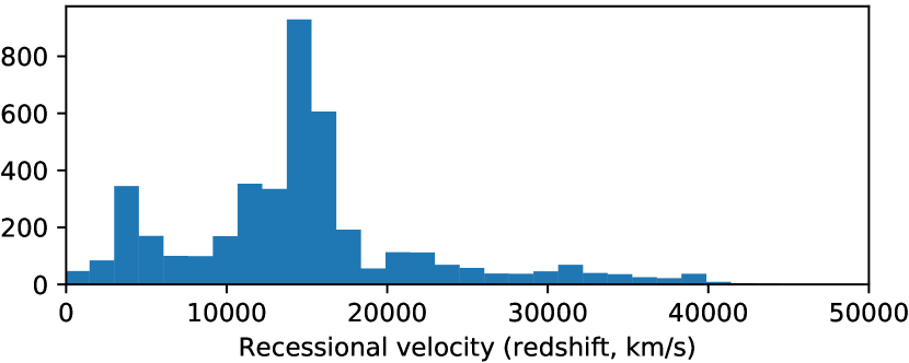
Refer to caption
(a)  
Refer to caption
(b)  
Refer to caption
(c)  
Refer to caption
Figure 6: (a) shows a histogram of velocities of galaxies from [20]. We model this data set using a Dirichlet process mixture, and evaluate the accuracy of SMC inference algorithms relative to a gold-standard, using AIDE and using a heuristic diagnostic based on measuring the average number of clusters in the approximating distribution and the gold-standard distribution. (b) shows results of AIDE. (c) shows result of the heuristic diagnostic. Both techniques indicate that rejuvenation kernels are important for fast convergence. Unlike the heuristic diagnostic, AIDE does not require custom design of a probe function for each model. We envision AIDE being used in concert with heuristic diagnostics like (c). In our experience, AIDE provides more conservative quantification of accuracy than heuristic diagnostics. The experiment was performed on a subsampled set of 40 data points from the data set in (a).