Co-clustering through Optimal Transport

Abstract

In this paper, we present a novel method for co-clustering, an unsupervised learning approach that aims at discovering homogeneous groups of data instances and features by grouping them simultaneously. The proposed method uses the entropy regularized optimal transport between empirical measures defined on data instances and features in order to obtain an estimated joint probability density function represented by the optimal coupling matrix. This matrix is further factorized to obtain the induced row and columns partitions using multiscale representations approach. To justify our method theoretically, we show how the solution of the regularized optimal transport can be seen from the variational inference perspective thus motivating its use for co-clustering. The algorithm derived for the proposed method and its kernelized version based on the notion of Gromov-Wasserstein distance are fast, accurate and can determine automatically the number of both row and column clusters. These features are vividly demonstrated through extensive experimental evaluations.

1 Introduction

Cluster analysis aims to gather data instances into groups, called clusters, where instances within one group are similar among themselves while instances in different groups are as dissimilar as possible. Clustering methods have become more and more popular recently due to their ability to provide new insights into unlabeled data that may be difficult or even impossible to capture for a human being. Clustering methods, however, do not take into account the possible existing relationships between the features that describe the data instances. For example, one may consider a data matrix extracted from text corpus where each document is described by the terms appearing in it. In this case, clustering documents may benefit from the knowledge about the correlation that exists between different terms revealing their probability of appearing in the same documents. This idea is the cornerstone of co-clustering (Hartigan, 1972; Mirkin, 1996) where the goal is to perform clustering of both data points and features simultaneously. The obtained latent structure of data is composed of blocks usually called co-clusters. Applications of co-clustering include but are not limited to recommendation systems (George & Merugu, 2005; Deodhar & Ghosh, 2010; Xu et al., 2012), gene expression analysis (Cheng et al., 2008; Hanisch et al., 2002) and text mining (Dhillon et al., 2003a; Wang et al., 2009). As a result, these methods are of an increasing interest to the data mining community.

Co-clustering methods are often distinguished into probabilistic methods (e.g., (Dhillon et al., 2003b; Banerjee et al., 2007; Nadif & Govaert, 2008; Wang et al., 2009; Shan & Banerjee, 2010)) and metric based (e.g., (Rocci & Vichi, 2008; Ding et al., 2006)) methods. Probabilistic methods usually make an assumption that data was generated as a mixture of probability density functions where each one of them corresponds to one co-cluster. The goal then is to estimate the parameters of the underlying distributions and the posterior probabilities of each co-cluster given the data. Metric based approaches proceed in a different way and rely on introducing and optimizing a criterion commonly taking into account intra- and inter-block variances. This criterion, in its turn, is defined using some proper metric function that describes the geometry of data in the most precise way possible. Both metric and probabilistic approaches are known to have their own advantages and limitations: despite being quite efficient in modeling the data distribution, probabilistic methods are computationally demanding and hardly scalable; metric methods are less computationally demanding but present the need to choose the “right” distance that uncovers the underlying latent co-clusters’ structure based on available data. Furthermore, the vast majority of co-clustering methods require the number of co-clusters to be set in advance. This is usually done using the computationally expensive exhaustive search over a large number of possible pairs of row and column clusters as in (Keribin et al., 2015; Wyse & Friel, 2012; Wyse et al., 2014).

In this paper, we address the existing issues of co-clustering methods described above by proposing a principally new approach that efficiently solves the co-clustering problem from both qualitative and computational points of view and allows the automatic detection of the number of co-clusters. We pose the co-clustering problem as the task of transporting the empirical measure defined on the data instances to the empirical measure defined on the data features. The intuition behind this process is very natural to co-clustering and consists in capturing the associations between instances and features of the data matrix. The solution of optimal transportation problem is given by a doubly-stochastic coupling matrix which can be considered as the approximated joint probability distribution of the original data. Furthermore, the coupling matrix can be factorized into three terms where one of them reflects the posterior distribution of data given co-clusters while two others represent the approximated distributions of data instances and features. We use these approximated distributions to obtain the final partitions. We also derive a kernelized version of our method that contrary to the original case, is based on an optimal transportation metric defined on the space of dissimilarity functions.

The main novelty of our work is two-fold. To the best of our knowledge, the proposed approach is a first attempt to apply entropy regularized optimal transport for co-clustering and to give its solution a co-clustering interpretation. While Wasserstein distance has already been adapted to design clustering algorithms (Cuturi & Doucet, 2014; Irpino et al., 2014), our idea is to concentrate our attention on the solution of the optimal transport given by the coupling matrix and not to minimize the quantization error with respect to (w.r.t.) Wasserstein distance. We also note that using entropy regularization leads to a very efficient algorithm that can be easily parallelized (Cuturi, 2013). Second, we show that under some plausible assumptions the density estimation procedure appearing from the use of the optimal transport results in the variational inference problem with the minimization of the reversed Kullback-Leibler divergence. The important implications of this difference w.r.t. other existing methods are explained in Section 3.

The rest of this paper is organized as follows. In Section 2, we briefly present the discrete version of the optimal transportation problem and its entropy regularized version. Section 3 proceeds with the description of the proposed approach, its theoretical analysis and algorithmic implementation. In Section 4, we evaluate our approach on synthetic and real-world data sets and show that it is accurate and substantially more efficient than the other state-of-the-art methods. Last section concludes the paper and gives a couple of hints for possible future research.

2 Background and notations

In this section, we present the formalization of the Monge-Kantorovich (Kantorovich, 1942) optimization problem and its entropy regularized version.

2.1 Optimal transport

Optimal transportation theory was first introduced in (Monge, 1781) to study the problem of resource allocation. Assuming that we have a set of factories and a set of mines, the goal of optimal transportation is to move the ore from mines to factories in an optimal way, i.e., by minimizing the overall transport cost.

More formally, given two empirical probability measures $\hat{\mu}_{S}=\frac{1}{N_{S}}\sum_{i=1}^{N_{S}}\delta_{x_{i}^{S}}$ and $\hat{\mu}_{T}=\frac{1}{N_{T}}\sum_{i=1}^{N_{T}}\delta_{x_{i}^{T}}$ defined as uniformly weighted sums of Dirac with mass at locations supported on two point sets $X_{S}=\{\bm{x}^{S}_{i}\in\mathbb{R}^{d}\}_{i=1}^{N_{S}}$ and $X_{T}=\{\bm{x}^{T}_{i}\in\mathbb{R}^{d}\}_{i=1}^{N_{T}}$, the Monge-Kantorovich problem consists in finding a probabilistic coupling $\gamma$ defined as a joint probability measure over $X_{S}\times X_{T}$ with marginals $\hat{\mu}_{S}$ and $\hat{\mu}_{T}$ that minimizes the cost of transport w.r.t. some metric $l:X_{s}\times X_{t}\rightarrow\mathbb{R}^{+}$:

$$\min_{\gamma\in\Pi(\hat{\mu}_{S},\hat{\mu}_{T})}\langle M,\gamma\rangle_{F}$$

where $\langle\cdot\text{,}\cdot\rangle_{F}$ is the Frobenius dot product, $\Pi(\hat{\mu}_{S},\hat{\mu}_{T})=\{\gamma\in\mathbb{R}^{N_{S}\times N_{T}}_{+}|\gamma\bm{1}=\hat{\mu}_{S},\gamma^{T}\bm{1}=\hat{\mu}_{T}\}$ is a set of doubly stochastic matrices and $M$ is a dissimilarity matrix, i.e., $M_{ij}=l(\bm{x}_{i}^{S},\bm{x}_{j}^{T})$, defining the energy needed to move a probability mass from $\bm{x}_{i}^{S}$ to $\bm{x}_{j}^{T}$. This problem admits a unique solution $\gamma^{*}$ and defines a metric on the space of probability measures (called the Wasserstein distance) as follows:

$$W(\hat{\mu}_{S},\hat{\mu}_{T})=\min_{\gamma\in\Pi(\hat{\mu}_{S},\hat{\mu}_{T})}\langle M,\gamma\rangle_{F}.$$

The Wasserstein distance has been successfully used in various applications, for instance: computer vision (Rubner et al., 2000), texture analysis (Rabin et al., 2011), tomographic reconstruction (I. Abraham & Carlier, 2016), domain adaptation (Courty et al., 2014), metric learning (Cuturi & Avis, 2014) and clustering (Cuturi & Doucet, 2014; Irpino et al., 2014). This latter application is of a particular interest as Wasserstein distance is known to be a very efficient metric due to its capability of taking into account the geometry of data through the pairwise distances between samples. The success of algorithms based on this distance is also due to (Cuturi, 2013) who introduced an entropy regularized version of optimal transport that can be optimized efficiently using matrix scaling algorithm. We present this regularization below.

2.2 Entropic regularization

The idea of using entropic regularization dates back to (Schrödinger, 1931). In (Cuturi, 2013), it found its application to the optimal transportation problem through the following objective function:

$$\min_{\gamma\in\Pi(\hat{\mu}_{S},\hat{\mu}_{T})}\langle M,\gamma\rangle_{F}-\frac{1}{\lambda}E(\gamma).$$

Second term $E(\gamma)=-\sum_{i,j}^{N_{S},N_{T}}\gamma_{i,j}\log(\gamma_{i,j})$ in this equation allows to obtain smoother and more numerically stable solutions compared to the original case and converges to it at the exponential rate (Benamou et al., 2015). Another advantage of entropic regularization is that it allows to solve optimal transportation problem efficiently using Sinkhorn-Knopp matrix scaling algorithm (Sinkhorn & Knopp, 1967).

In the next section, we explain the main underlying idea of our approach that consists in associating data instances with features through regularized optimal transport.

3 Co-clustering through optimal transport

In this section we show how the co-clustering problem can be casted in a principally new way and then solved using the ideas from the optimal transportation theory.

3.1 Problem setup

Let us denote by $X$ and $Y$ two random variables taking values in the sets $\{\bm{x}_{r}\}_{r=1}^{n}$ and $\{\bm{y}_{c}\}_{c=1}^{d}$, respectively, where subscripts $r$ and $c$ correspond to rows (instances) and columns (features). Similar to (Dhillon et al., 2003b), we assume that the joint probability distribution between $X$ and $Y$ denoted by $p(X,Y)$ is estimated from the data matrix $\mathcal{A}\in\mathbb{R}^{n\times d}$. We further assume that $X$ and $Y$ consist of instances that are distributed w.r.t. probability measures $\mu_{r}$, $\mu_{c}$ supported on $\Omega_{r},\Omega_{c}$ where $\Omega_{r}\subseteq\mathbb{R}^{d}$ and $\Omega_{r}\subseteq\mathbb{R}^{n}$, respectively.

The problem of co-clustering consists in jointly grouping the set of features and the set of instances into homogeneous blocks by finding two assignment functions $C_{r}$ and $C_{c}$ that map as follows: $C_{r}:\{\bm{x}_{1},\dots,\bm{x}_{n}\}\rightarrow\{\hat{x}_{1},\dots,\hat{x}_{g}\}$, $C_{c}:\{\bm{y}_{1},\dots,\bm{y}_{d}\}\rightarrow\{\hat{y}_{1},\dots,\hat{y}_{m}\}$ where $g$ and $m$ denote the number of row and columns clusters, and discrete random variables $\hat{X}$ and $\hat{Y}$ represent the partitions induced by $X$ and $Y$, i.e., $\hat{X}=C_{r}(X)=$ and $\hat{Y}=C_{c}(Y)$. To use discrete optimal transport, we also define two empirical measures $\hat{\mu}_{r}$ and $\hat{\mu}_{c}$ based on $X$ and $Y$ as follows: $\hat{\mu}_{r}=\frac{1}{n}\sum_{i=1}^{n}\delta_{\bm{x}_{i}}$ and $\hat{\mu}_{c}=\frac{1}{m}\sum_{i=1}^{m}\delta_{\bm{y}_{i}}$. We are now ready to present our method.

3.2 Proposed approach

The main underlying idea of our approach is to use the optimal transportation presented above to find a probabilistic coupling of the empirical measures defined based on rows and columns of a given data matrix. More formally, for some fixed $\lambda>0$ we solve the co-clustering problem through the following optimization procedure:

$$\gamma^{*}_{\lambda}=\rm argmin_{\gamma\in\Pi(\hat{\mu}_{r},\hat{\mu}_{c})}\langle M,\gamma\rangle_{F}-\frac{1}{\lambda}E(\gamma),$$ (1)

where the matrix $M$ is computed using the Euclidean distance, i.e., $M_{ij}=\|\bm{x}_{i}-\bm{y}_{j}\|^{2}$. The elements of the resulting matrix $\gamma^{*}_{\lambda}$ provides us with the weights of associations between instances and features: similar instances and features correspond to higher values in $\gamma^{*}_{\lambda}$. Our intuition is to use these weights to identify the most similar sets of rows and columns that should be grouped together to form co-clusters.

Following (Benamou et al., 2015), this optimization problem can be equivalently rewritten in the following way:

$$\min_{\gamma\in\Pi(\hat{\mu}_{r},\hat{\mu}_{c})}\langle M,\gamma\rangle_{F}-\frac{1}{\lambda}E(\gamma)=\frac{1}{\lambda}\min_{\gamma\in\Pi(\hat{\mu}_{r},\hat{\mu}_{c})}\text{KL}(\gamma\|\xi_{\lambda}),$$

where $\xi_{\lambda}=e^{-\lambda M}$ is the Gibbs kernel.

Finally, we can rewrite the last expression as follows:

$$\min_{\gamma\in\Pi(\hat{\mu}_{r},\hat{\mu}_{c})}\text{KL}(\gamma\|\xi_{\lambda})=\min_{\gamma\in\mathcal{C}}\text{KL}(\gamma\|\xi_{\lambda}),$$

where $\mathcal{C}=\mathcal{C}_{1}\cap\mathcal{C}_{2}$ is the intersection of closed convex subsets given by $\mathcal{C}_{1}=\{\gamma\in\mathbb{R}^{d\times d}|\gamma\bm{1}=\hat{\mu}_{r}\}$ and $\mathcal{C}_{2}=\{\gamma\in\mathbb{R}^{d\times d}|\gamma^{T}\bm{1}=\hat{\mu}_{c}\}$. The solution of the entropy regularized optimal transport can be obtained using Sinkhorn-Knopp algorithm and has the following form (Benamou et al., 2015):

$$\gamma^{*}_{\lambda}=\text{diag}(\bm{\alpha})\xi_{\lambda}\text{diag}(\bm{\beta}),$$ (2)

where $\bm{\alpha}$ and $\bm{\beta}$ are the scaling coefficients of the Gibbs kernel $\xi_{\lambda}$.

In what follows, we show that under some plausible assumptions, we can interpret these two vectors as approximated rows and columns probability density functions.

3.3 Connection to variational inference

In order to justify our approach from the theoretical point of view, we first explain how the obtained solution $\gamma^{*}$ can be used for co-clustering. As mentioned in (Dhillon et al., 2003b) and later in (Banerjee et al., 2007), the co-clustering can be seen as a density estimation problem where the goal is to approximate the real density $p(X,Y)$ by a simpler one depending on the obtained co-clustering in a way that it preserves the loss in the mutual information given by $I(X,Y)-I(\hat{X},\hat{Y})$ where $I(X,Y)=\int_{XY}p(x,y)\log\frac{p(x,y)}{p(x)p(y)}dxdy$ is the mutual information. This quantity is further shown to be equal to the Kullback-Leibler divergence between the original distribution $p(X,Y)$ and $q(X,Y)$ where the latter has the following form:

$$q(x,y)=p(y|\hat{y})p(\hat{x},\hat{y})p(x|\hat{x}).$$

From this point, one may instantly see that the solution of the optimal transport problem $\gamma^{*}$ has a very similar form as it also represents the joint probability distribution that approximates the original probability distribution $p(x,y)$ given by the Gibbs measure $\xi_{\lambda}$ and also factorizes into three terms. The most important difference, however, lies in the asymmetry of the KL divergence: while (Dhillon et al., 2003b) and (Banerjee et al., 2007) concentrate on minimizing $\text{KL}(p(X,Y)\|q(X,Y))$, our idea is different and consists in minimizing $\text{KL}(q(X,Y)\|p(X,Y))$. This approach is known in the literature as the variational inference (Bishop, 2006) and exhibits a totally different behaviour compared to the minimization of $\text{KL}(p(X,Y)\|q(X,Y))$. As shown by (Bishop, 2006), in variational inference the estimated distribution $q(X,Y)$ concentrates on the modes of data and remains compact, while the minimizer of $\text{KL}(p(X,Y)\|q(X,Y))$ tends to cover the whole surface of the original density and to overestimate its support. As $X$, $Y$ and $\hat{X}$ and $\hat{Y}$ represent the observed and unobserved variables, respectively, the natural goal is to try to estimate the distribution $p(X,Y|\hat{X},\hat{Y})$ of the data given the obtained co-clusters by the simpler variational distribution $q(X,Y)$. However, as the maximisation of $p(X,Y|\hat{X},\hat{Y})$ is computationally impossible, it is common to introduce a free distribution $q(\cdot,\cdot)$ on the parameters $\widehat{X}$ and $\widehat{Y}$ in order to obtain the following decomposition:

$$\!\log p(X,Y)\!=\!\mathcal{L}(q(\hat{X},\hat{Y}))\!+\!\text{KL}(q(\hat{X},\hat{Y})\|p(\hat{X},\hat{Y}|X,Y)),$$

where the lower bound

$$\mathcal{L}(q(\hat{X},\hat{Y}))=\int_{\hat{x}\in\hat{\mathcal{X}}}\int_{\hat{y}\in\hat{\mathcal{Y}}}q(\hat{x},\hat{y})\log\frac{p(x,y,\hat{x},\hat{y})}{q(\hat{x},\hat{y})}d\hat{x}d\hat{y}$$

is maximized when the KL divergence is minimized.

Now, if we assume that $p(\hat{X},\hat{Y}|X,Y)$ follows the Gibbs distribution, i.e. $p(\hat{X},\hat{Y}|X,Y)\propto e^{-\lambda M(x,y)}$, we can consider the original formulation of the regularized optimal transport as the variational inference problem:

$$\min_{q}\text{KL}(q(\hat{X},\hat{Y})\|p(\hat{X},\hat{Y}|X,Y))=\min_{\gamma}\text{KL}(\gamma\|\xi_{\lambda}),$$

where the optimal coupling $\gamma$ equals to the estimated joint probability $q(\hat{X},\hat{Y})$.

At this point, we know that the coupling matrix can be seen as an approximation to the original unknown posterior density function but the question how one can use it to obtain the clustering of rows and columns has not been answered yet. In order to solve the variational inference problem, it is usually assumed that the variables $\hat{x},\hat{y}$ are independent and thus the variational distribution $q(\hat{x},\hat{y})$ factorizes as $q(\hat{x},\hat{y})=q(\hat{x})q(\hat{y})$. This assumption, however, goes against the whole idea of co-clustering that relies on the existence of a deep connection between these two variables.

To this end, we propose to consider the factorization of $q(\hat{x},\hat{y})$ that has the following form

$$q(\hat{x},\hat{y})=q(x)q(\hat{x},\hat{y}|x,y)q(y).$$

This particular form follows the idea of structured stochastic variational inference proposed in (Hoffman & Blei, 2015) where a term depicting the conditional distribution between hidden and observed variables is added to the fully factorized traditional setting presented above. As stated in (Hoffman & Blei, 2015), this term allows arbitrary dependencies between observed and hidden variables which can increase the fidelity of the approximation.

Following (Bishop, 2006), the optimal estimated densities $q(x)$ and $q(y)$ are controlled by the direction of the smallest variance of $p(x)$ and $p(y)$ respectively. Furthermore, $q(x)$ and $q(y)$ are proportional to the joint densities $p(\hat{y},y)$ and $p(\hat{x},x)$, i.e., $q(x)\propto p(\hat{y},y)$ and $q(y)\propto p(\hat{x},x)$. Bearing in mind the equivalence between $\gamma^{*}_{\lambda}$ and $q(\hat{x},\hat{y})$, this brings us to the following important conclusions: (1) the matrices $\text{diag}(\bm{\alpha})$ and $\text{diag}(\bm{\beta})$ can be seen as the approximated densities $p(\hat{Y},Y)$ and $p(\hat{X},X)$; (2) vectors $\bm{\alpha}$ and $\bm{\beta}$ represent the approximated densities $p(X)$ and $p(Y)$ obtained by summing $X$ and $Y$ out of $p(\hat{X},X)$ and $p(\hat{Y},Y)$, respectively.

According to (Laird, 1978), the non-parametric estimate of the mixing distribution is a piecewise step function where the number of steps depend on the number of components in the mixture. In the cluster analysis, we can assume that $p(X)$ and $p(Y)$ consist of $g$ and $m$ components, respectively. Then, our goal is to detect these steps based on the estimates given by $\bm{\alpha}$ and $\bm{\beta}$ to obtain the desired partitions.

3.4 Kernelized version and Gromov-Wasserstein distance

In this part, we introduce the kernelized version of our method and compare it to the original formulation of our algorithm. In order to proceed, we first define two similarity matrices $K_{r}\in\mathbb{R}^{n\times n}$ and $K_{c}\in\mathbb{R}^{d\times d}$ associated to empirical measures $\hat{\mu}_{r},\hat{\mu}_{c}$ thus forming metric-measure spaces as in (Mémoli, 2011). Matrices $K_{r}$ and $K_{c}$ are defined by calculating the pairwise distances or similarities between rows and columns, respectively, without the restriction of them being positive or calculated based on a proper distance function satisfying the triangle inequality. The entropic Gromov-Wasserstein discrepancy in this case is defined as follows (Peyré et al., 2016):

$$\text{GW}(K_{r},K_{c},\hat{\mu}_{r},\hat{\mu}_{c})=\min_{\gamma\in\Pi_{\hat{\mu}_{r},\hat{\mu}_{c}}}\Gamma_{K_{r},K_{c}}(\gamma)-\lambda E(\gamma)$$

$$=\min_{T\in\Pi_{\hat{\mu}_{r},\hat{\mu}_{c}}}\sum_{i,j,k,l}L(K_{r_{i,j}},K_{c_{k,l}})\gamma_{i,j}\gamma_{k,l}-\lambda E(\gamma).$$

where $\gamma$ is a coupling matrix between two similarity matrices and $L:\mathbb{R}\times\mathbb{R}\rightarrow\mathbb{R}_{+}$ is an arbitrary lost-function, usually the quadratic-loss or Kullback-Leibler divergence.

Based on this definition, one may define the problem of the entropic Gromov-Wasserstein barycenters for similarity or distance matrices $K_{r}$ and $K_{c}$ as follows:

$$\min_{K,\gamma_{r},\gamma_{c}}\sum_{i=\{r,c\}}\varepsilon_{i}\Gamma_{K,K_{i}}(\gamma_{i})-\lambda E(\gamma_{i})$$ (3)

where $K$ is the computed barycenter and $\gamma_{r}\in\Pi_{\hat{\mu},\hat{\mu}_{r}}$, $\gamma_{c}\in\Pi_{\hat{\mu},\hat{\mu}_{c}}$ are the coupling matrices that align it with $K_{r}$ and $K_{c}$, respectively. $\varepsilon_{i}$ are the weighting coefficients summing to one, i.e., $\sum_{i=\{r,c\}}\varepsilon_{i}=1$ that determine our interest in more accurate alignment between $K_{r}$ and $K$ or $K_{c}$ and $K$.

The intuition behind this optimization procedure for co-clustering with respect to original formulation given in (1) is the following: while in (1) we align rows with columns directly, in (3) our goal is to do it via an intermediate representation given by the barycenter $K$ that is optimally aligned with both $K_{r}$ and $K_{c}$. In this case, we obtain the solutions $\gamma_{r}$ and $\gamma_{c}$ that, similar to (2), can be decomposed as follows:

$$\gamma_{r}^{*}=\text{diag}(\bm{\alpha_{r}})\xi_{r}\text{diag}(\bm{\beta_{r}}),\,\gamma_{c}^{*}=\text{diag}(\bm{\alpha_{c}})\xi_{c}\text{diag}(\bm{\beta_{c}})$$

where $\xi_{r}=e^{-\lambda M_{r}}$ and $\xi_{c}=e^{-\lambda M_{c}}$ are Gibbs kernels calculated between the barycenter and row and column similarity matrices using any arbitrary loss-function $L$ as explained before. Finally, based on the analysis presented above, we further use vectors $\bm{\beta_{r}}$ and $\bm{\beta_{c}}$ to derive row and column partitions.

3.5 Detecting the number of clusters

In order to detect the steps (or jumps) in the approximated marginals, we propose to adapt a procedure introduced in (Matei & Meignen, 2012) for multiscale denoising of piecewise smooth signals. This method is of particular interest for us as it determines the significant jumps in the vectors $\bm{\alpha}$ and $\bm{\beta}$ without knowing their number and location, nor a specific threshold to decide the significance of a jump. As the proposed procedure deals with non-decreasing functions, we first sort the values of $\bm{\alpha}$ and $\bm{\beta}$ in the ascending order. Since the procedure is identical for both vectors, we only describe it for the vector $\bm{\alpha}$.

We consider that the elements $\{\alpha_{i}\}_{i=1}^{n}$ of $\bm{\alpha}$ are the local averages of a piecewise continuous function $v:[0,1[\subset\mathbb{R}\rightarrow\mathbb{R}$ on the intervals $I^{n}_{i}=[i/n,(i+1)/n[$ defined by the uniform subdivision of step $1/n$ of the interval $[0,1[$. More precisely: $\alpha^{n}_{i}=n\int_{I^{n}_{i}}v(t)dt,i=0,\ldots,n-1$. The detection strategy is based on the following cost function: $F(I^{n}_{i})=\sum_{l=i-1}^{i}|\alpha^{n}_{l+1}-\alpha^{n}_{l}|$ defined for each interval. Therefore, we get the list of the interval suspicious to contain a jump for the subdivision of order $n$ as follows:

$$L^{n}=\{i^{*};i^{*}=\rm argmax_{i}F(I^{n}_{i})\}.$$

This detection should be refined in order to get only significant jumps in our vector $\bm{\alpha}.$ To this end we use the multiscale representation of $\bm{\alpha}$ as in (Harten, 1989) and we perform this detection on each scale. On the first scale, we get a coarse version of $\bm{\alpha}$ by averaging:

$$\alpha^{n/2}_{i}=\frac{1}{2}(\alpha^{n}_{2i}+\alpha^{n}_{2i+1}),i=0,\ldots,n/2-1.$$

Now, by considering the coarse version of $\bm{\alpha}$, we obtain a second list $L^{n/2}$ of suspicious intervals as before. After that, these two lists merge in the list $L_{\text{jumps}}$ as follows: a jump will be considered in the interval $I^{n}_{2i}$ or $I^{n}_{2i+1}$ if the interval $I^{n/2}_{i}$ is also detected as suspicious at the coarse scale. This procedure is iterated $[\log_{2}n]$ times and a jump is observed if a chain of detection exists from fine to coarse scales. Finally, the number of clusters is obtained by $g=|L_{\text{jumps}}|+1$.

3.6 Algorithmic implementation

We now briefly summarize the main steps of both CCOT and CCOT-GW methods and discuss their peculiarities with respect to each other. The pseudocode of both approaches in Matlab are presented in Algorithm 1 and Algorithm 2, respectively.

CCOT

First step of our algorithm consists in calculating the cost matrix $M$ and using it to obtain the optimal coupling matrix $\gamma^{*}_{\lambda}$ by applying the regularized optimal transport. In order to calculate $M$, row and column instances should both lie in a space of the same dimension. This condition, however, is verified only if the matrix $\mathcal{A}$ is squared which occurs rarely in the real-world applications. To overcome this issue, we first subsample the original data set $\mathcal{A}$ in a way that allows us to equalize the number of rows and columns and operate with two sets of the same dimension. If we assume that $n>d$ then this new reduced data set is denoted by $D\in\mathbb{R}^{d\times d}$. We repeat the sampling procedure until every individual is picked at least once.

The next step is to perform for each $i=1,\dots,n_{s}$ the jump detection on the sorted vectors $\bm{\alpha}_{i}$ and $\bm{\beta}_{i}$ to obtain two lists of the jumps locations $L_{\text{jumps}}^{\alpha_{i}}$ and $L_{\text{jumps}}^{\beta_{i}}$ and to define the number of row and column clusters $g$ and $m$. By using them, we obtain the resulting row partition:

$$C_{r}^{i}(\bm{x}_{r})=\left\{\begin{array}[]{ll}1,\;\ r\leq L_{\text{jumps}}^{\alpha_{i}}(1)\\ \dots\\ k,\;\ L_{\text{jumps}}^{\alpha_{i}}(k-1)<r\leq L_{\text{jumps}}^{\alpha_{i}}(k)\\ \dots\\ |L_{\text{jumps}}^{\alpha_{i}}|+1,\;\ r>L_{\text{jumps}}^{\alpha_{i}}(|L_{\text{jumps}}^{\alpha_{i}}|).\end{array}\right.$$

The partition for columns $C_{c}^{i}(\bm{y}_{c})$ is obtained in the same way. Finally, we apply the majority vote over all samples partitions to obtain $C_{r}$ and $C_{c}$. Regarding complexity, both Sinkhorn-Knopp algorithm used to solve the regularized optimal transport (Knight, 2008) and the proposed jump detection techniques are known to converge at the linear rate multiplied by the number of samples, i.e., $\mathcal{O}(n_{s}d)$. On the other hand, the calculation of modes of the clustering obtained on the generated samples for both features and data instances has the complexity $\mathcal{O}(n_{s}(n+d))$. In the end, the complexity of the whole algorithm is $\mathcal{O}(n_{s}(n+d))$. We also note that in the real-world applications, we usually deal with scenarios where $n\gg d$ (“big data”) or $d\ll n$ (“small” data) thus reducing the overall complexity to $\mathcal{O}(n_{s}n)$ and $\mathcal{O}(n_{s}d)$, respectively. This makes our approach even more computationally attractive.

Input :

$\mathcal{A}$ - data matrix, $\lambda$ - regularization parameter, $n_{s}$ - number of sampling

Output :

$C_{r},C_{c}$ - partition matrices for rows and columns, $g,m$ - number of row and column clusters

$\mathtt{[n,d]=size(Z)}$

for $i=1$ to $n_{s}$ do

       $\mathtt{D_{i}=datasample(Z,d)}$   $\mathtt{M_{i}\leftarrow pdist2(D_{i},D_{i}^{T})}$  $\mathtt{[\bm{\alpha}_{i},\bm{\beta}_{i},\gamma^{*}]\leftarrow optimal\_transport(M_{i},\lambda)}$  $\mathtt{[L_{\text{jumps}}^{\alpha_{i}},C_{r}^{i},g]\leftarrow jump\_detection(sort(\bm{\alpha}_{i}))}$   $\mathtt{[L_{\text{jumps}}^{\beta_{i}},C_{c}^{i},m]\leftarrow jump\_detection(sort(\bm{\beta}_{i}))}$  

$\mathtt{C_{r}\leftarrow mode(C_{r}^{i})}$  $\mathtt{C_{c}\leftarrow mode(C_{c}^{i})}$ 

Algorithm 1 Co-clustering through Optimal Transport (CCOT)

CCOT-GW

As it can be seen from Algorithm 2, CCOT-GW allows to overcome the important disadvantage of CCOT that consists in the need to perform sampling to cluster all data objects. On the other hand, the computational complexity of CCOT is only $\mathcal{O}(n_{s}d)$, while for CCOT-GW it scales as $\mathcal{O}(n^{2}d+d^{2}n)$. We also note that CCOT-GW offers a great flexibility in terms of the possible data representation used at its input. One may easily consider using any arbitrary kernel function to calculate similarity matrices or even learn them beforehand using multiple-kernel learning approaches.

Input :

$\mathcal{A}$ - data matrix, $\lambda$ - regularization parameter, $\varepsilon_{r}$, $\varepsilon_{c}$ - weights for barycenter calculation

Output :

$C_{r},C_{c}$ - partition matrices for rows and columns, $g,m$ - number of row and column clusters

$\mathtt{K_{r}\leftarrow pdist2(Z,Z)}$

$\mathtt{K_{c}\leftarrow pdist2(Z^{T},Z^{T})}$

$\mathtt{[\bm{\beta}_{r},\bm{\beta}_{c},\gamma^{*}_{r},\gamma^{*}_{c}]\leftarrow gw\_barycenter(K_{r},K_{c},\lambda,\varepsilon_{r},\varepsilon_{c})}$

$\mathtt{[L_{\text{jumps}}^{\beta_{r}},C_{r},g]\leftarrow jump\_detection(sort(\bm{\beta}_{r}))}$

$\mathtt{[L_{\text{jumps}}^{\beta_{c}},C_{c},m]\leftarrow jump\_detection(sort(\bm{\beta}_{c}))}$

Algorithm 2 Co-clustering through Optimal Transport with Gromov-Wasserstein barycenters (CCOT-GW)

Table 2: Mean ($\pm$ standard-deviation) of the co-clustering error (CCE) obtained for all configurations. “-” indicates that the algorithm cannot find a partition with the requested number of co-clusters. P-values obtained using the non-parametric test of Wilcoxon (Wilcoxon, 1945) that imply significant differences are printed in bold (significance level of 0.05).

Data set	Algorithms
	K-means	NMF	DKM	Tri-NMF	GLBM	ITCC	RBC	CCOT	CCOT-GW
D1	$\mathbf{.018\pm{.003}}$	$.042\pm{.037}$	$.025\pm{.048}$	$.082\pm{.063}$	$.021\pm{.011}$	$.021\pm{.001}$	$.017\pm{.045}$	$.018\pm{.013}$	$\mathbf{.004\pm{.002}}$
D2	$.072\pm{.044}$	$.083\pm{.063}$	$.038\pm{.000}$	$.052\pm{.065}$	$.032\pm{.041}$	$.047\pm{.042}$	$.039\pm{.052}$	$.023\pm{.036}$	$\mathbf{.011\pm{.056}}$
D3	–	–	$.310\pm{.000}$	–	$.262\pm{.022}$	$.241\pm{.031}$	–	$.031\pm{.027}$	$\mathbf{.008\pm{.001}}$
D4	$.126\pm{.038}$	–	$.145\pm{.082}$	–	$.115\pm{.047}$	$.121\pm{.075}$	$.102\pm{.071}$	$.093\pm{.032}$	$\mathbf{.079\pm{.031}}$

4 Experimental evaluations

In this section, we provide empirical evaluation for the proposed algorithms.

4.1 Synthetic data

Simulation setting

We simulate data following the generative process of the Gaussian Latent Block Models (for details see (Govaert & Nadif, 2013)) and we consider four scenarios with different number of co-clusters, degree of separation and size. Table 1 and Figure 1 present the characteristics of theta simulated data sets and their visualization showing the different co-clustering structures.

Table 1: Size ($n\times d$), number of co-clusters ($g\times m$), degree of overlapping ([+] for well-separated and [++] for ill-separated co-clusters) and the proportions of co-clusters for simulated data sets.

Data set	$n\times d$	$g\times m$	Overlapping	Proportions
D1	$600\times 300$	$3\times 3$	[+]	Equal
D2	$600\times 300$	$3\times 3$	[+]	Unequal
D3	$300\times 200$	$2\times 4$	[++]	Equal
D4	$300\times 300$	$5\times 4$	[++]	Unequal

(a) D2

(b) D3

(c) D4

Figure 1: D2, D3 and D4 reorganized w.r.t. the true partitions.

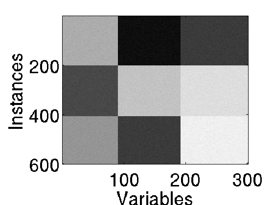
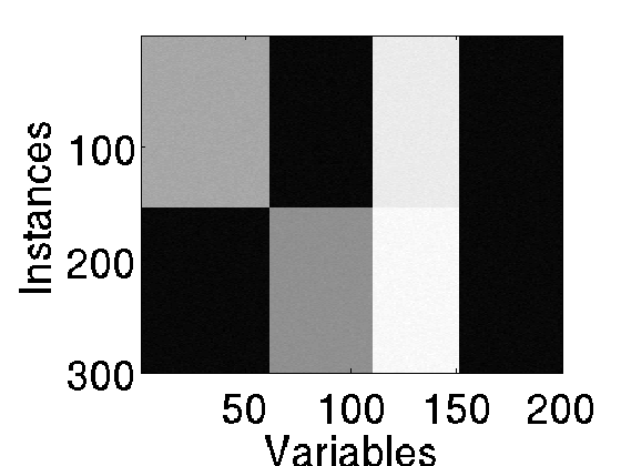
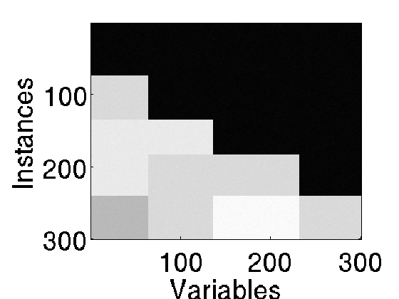
We use several state-of-the-art co-clustering algorithms as baselines including ITCC (Dhillon et al., 2003b), Double K-Means (DKM) (Rocci & Vichi, 2008), Orthogonal Nonnegative Matrix Tri-Factorizations (ONTMF) (Ding et al., 2006), the Gaussian Latent Block Models (GLBM) (Nadif & Govaert, 2008; Govaert & Nadif, 2013) and Residual Bayesian Co-Clustering (RBC) (Shan & Banerjee, 2010). We also report the results of K-means and NMF, run on both modes of the data matrix, as clustering baseline. To assess the performance of all compared methods, we compute the co-clustering error (CCE) (Patrikainen & Meila, 2006) defined as follows:

$$\text{CCE}((\mathbf{z},\mathbf{w}),(\hat{\mathbf{z}},\hat{\mathbf{w}}))=e(\mathbf{z},\hat{\mathbf{z}})+e(\mathbf{w},\hat{\mathbf{w}})-e(\mathbf{z},\hat{\mathbf{z}})\times e(\mathbf{w},\hat{\mathbf{w}}),$$

where $\hat{\mathbf{z}}$ and $\hat{\mathbf{w}}$ are the partitions of instances and variables estimated by the algorithm; $\mathbf{z}$ and $\mathbf{w}$ are the true partitions and $e(\mathbf{z},\hat{\mathbf{z}})$ (resp. $e(\mathbf{w},\hat{\mathbf{w}})$) denotes the error rate, i.e., the proportion of misclassified instances (resp. features).

For all configurations, we generate 100 data sets and compute the mean and standard deviation of the CCE over all sets. As all the approaches we compared with are very sensitive to the initialization, we run them $50$ times with random initializations and retain the best result according to the corresponding criterion. RBC is initialized with K-means. Regarding CCOT we set $n_{s}$ to $1000$ for all configurations except D4 which has the same number of rows and columns, and therefore does not require any sampling. For CCOT-GW, we use Gaussian kernels for both rows and columns with $\sigma$ computed as the mean of all pairwise Euclidean distances between vectors (Kar & Jain, 2011). Finally, we let both CCOT and CCOT-GW detect automatically the number of co-clusters, while for all other algorithms we set the number of clusters to its true value.

Co-clustering performance

We report the mean (and standard deviation) of co-clustering errors obtained in Table 2. Based on these results, we observe that on D1, which has a clear block structure, all algorithms perform equally well, however CCOT-GW gives the best results, closely followed by CCOT and K-means. Regarding D2, D3 and D4, which have more complicated structure than D1, both CCOT and CCOT-GW significantly outperform all other algorithms and this difference is all the more important on D3 and D4 where some of the compared algorithms are unable to find a partition with the desired number of clusters.

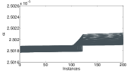
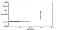
Furthermore, we argued that one of the strengths of our method is its ability to detect automatically the number of co-clusters by applying a jump detection algorithm on $\bm{\alpha}$ and $\bm{\beta}$. From Figure 2 one can observe that the plots of these vectors, obtained with CCOT, with their elements sorted in the ascending order reveal clear steps that correspond to the correct number of clusters and also illustrate their proportions and the degree of overlapping. The same observation is valid for CCOT-GW. Both approaches correctly identified the number of clusters in most cases and CCOT is slightly more accurate than CCOT-GW when the proportions of co-clusters are unbalanced.

(a)

(b)

Data Set	CCOT		CCOT-GW
	$g$	$m$	$g$	$m$
D1	$\mathbf{100}$	$\mathbf{100}$	$98$	$100$
D2	$\mathbf{83}$	$\mathbf{97}$	$81$	$72$
D3	$\mathbf{99}$	$\mathbf{98}$	$93$	$97$
D4	$\mathbf{73}$	$86$	$70$	$\mathbf{87}$

(c)

Figure 2: Vectors (a) $\bm{\alpha}$ and (b) $\bm{\beta}$ obtained with CCOT on D3. (c) Number of times CCOT and CCOT-GW correctly detect the number of co-clusters ($g$ and $m$) over 100 trials.

To summarize, CCOT and CCOT-GW outperform all the other baselines for the considered data structures and present two important advantages: (1) they do not suffer from the initialization issues, (2) they are able to detect automatically the number co-clusters.

4.2 MovieLens

Data and setting

MovieLens-100K is a popular benchmark data set that consists of user-movie ratings, on a scale of one to five, collected from a movie recommendation service gathering 100,000 ratings from 943 users on 1682 movies. In the context of co-clustering, our goal is to find homogeneous subgroups of users and films in order to further recommend previously unseen movies that were highly rated by the users from the same group.

We set the regularization parameters for CCOT and CCOT-GW using the cross-validation; the number of samplings for CCOT is set to $500$ (as the dimensions of the data set are quite balanced); the weights for the barycenter in CCOT-GW are set to $\varepsilon=(0.5,0.5)$.

Results

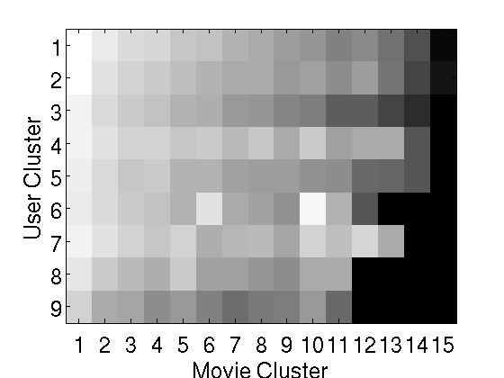
In what follows we only present figures and results obtained by CCOT-GW as both algorithms return the same number of blocks and the partitions are almost identical (with a normalized mutual information between partitions above $0.8$). CCOT-GW automatically detects a structure consisting of $9\times 15$ blocks, that corresponds to 9 user clusters and 15 movie clusters. From Figure 3, one can observe that the users and the movies are almost equally distributed across clusters, except for two user and three movie clusters which have a larger size than others.

(a)

(b)

Figure 3: Distribution of the number of (a) users and (b) movies across the clusters obtained with CCOT-GW.

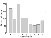
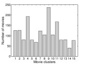
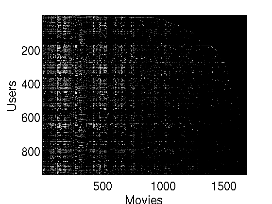
Figure 4 shows the original data set as well as a summarized version where each block is represented by its mean rating value (the lighter the block, the higher the ratings), revealing a structure into homogeneous groups. One can observe that the first movie cluster consists of films for which all users agree on giving high ratings (most popular movies) while the last movie cluster consists of the movies with very low ratings. We also report the 5 best rated movies in those two clusters in Table 3. One can easily see that popular movies, such that both Star Wars episodes are in M1 while M5 is composed of movies that were less critically acclaimed.

(a)

(b)

Figure 4: (a) MovieLens matrix; (b) the matrix summarized by the mean rating (0 ratings are excluded) for each block obtained with CCOT-GW. Darker shades indicate lower values.

Table 3: Top 5 of movies in clusters M1 and M15.

M1	M15
Star Wars (1977)	Amytiville: A New Generation (1993)
The Lion King (1994)	Amytiville: It’s About Time (1992)
Return of the Jedi (1983)	Ninjas: High Noon at Mega Mountain (1998)
Contact (1997)	Sudden Manhattan (1996)
Raiders of the lost ark (1981)	Dream Man (1995)

We can make similar observations for the interpretation of user clusters. For instance, the last two user clusters include users that tend to give less good ratings to movies than the average population. Also, we note that block $(6,10)$ corresponds to users who liked movies from M10 better than the rest of the users. These observations are also very similar to the results reported by (Banerjee et al., 2007), where the authors proposed a detailed study of a $10\times 20$ blocks structure for this data set. Additional results can be found in the Supplementary material.

5 Conclusions and future perspectives

In this paper we presented a novel approach for co-clustering based on the entropy regularized optimal transport. Our method is principally different from other co-clustering methods and consists in finding a probabilistic coupling of the empirical measures defined based on the data instances and features. We showed how this procedure can be seen as the variational inference problem and that the inferred distribution can be used to obtain the row and feature partitions. The resulting algorithm is not only more accurate than other state-of-the-art methods but also fast and capable of automatically detecting the number of co-clusters. We also presented an extended version of our algorithm that makes use of the optimal transportation distance defined on similarity matrices associated to the rows’ and columns’ empirical measures.

In the future, our work can be continued in multiple directions. First, we would like to extend our method in order to deal with the online setting where the goal is to classify a new previously unseen observation without the need to do the co-clustering of the data set that includes it. This can be done using a recent approach proposed in (Perrot et al., 2016) that allows to update the learned coupling matrix using the out-of-sample observations without recomputing it using all the data. We believe that this extension will make our algorithm attractive for the exploitation in real-time industrial recommendation systems due to its computational efficiency. We would also like to study the generalization properties of our algorithm in a spirit similar to the results obtained in (Maurer & Pontil, 2010). This latter work presents a rare case where the generalization bounds are derived for some famous unsupervised learning algorithms.

References

- Banerjee et al. (2007) Banerjee, Arindam, Dhillon, Inderjit, Ghosh, Joydeep, Merugu, Srujana, and Modha, Dharmendra S. A generalized maximum entropy approach to bregman co-clustering and matrix approximation. Journal of Machine Learning Research, 8:1919–1986, December 2007.
- Benamou et al. (2015) Benamou, Jean-David, Carlier, Guillaume, Cuturi, Marco, Nenna, Luca, and Peyré, Gabriel. Iterative Bregman Projections for Regularized Transportation Problems. SIAM Journal on Scientific Computing, 2(37):A1111–A1138, 2015.
- Bishop (2006) Bishop, Christopher M. Pattern Recognition and Machine Learning (Information Science and Statistics). Springer-Verlag New York, Inc., 2006.
- Cheng et al. (2008) Cheng, Kin-On, Law, Ngai-Fong, Siu, Wan-Chi, and Liew, Alan W. Identification of coherent patterns in gene expression data using an efficient biclustering algorithm and parallel coordinate visualization. BMC Bioinformatics, 9:210, 2008.
- Courty et al. (2014) Courty, Nicolas, Flamary, Rémi, and Tuia, Devis. Domain adaptation with regularized optimal transport. In Proceedings ECML/PKDD 2014, pp. 1–16, 2014.
- Cuturi (2013) Cuturi, Marco. Sinkhorn distances: Lightspeed computation of optimal transport. In Proceedings NIPS, pp. 2292–2300, 2013.
- Cuturi & Avis (2014) Cuturi, Marco and Avis, David. Ground metric learning. Journal of Machine Learning Research, 15(1):533–564, 2014.
- Cuturi & Doucet (2014) Cuturi, Marco and Doucet, Arnaud. Fast computation of wasserstein barycenters. In Proceedings ICML, pp. 685–693, 2014.
- Deodhar & Ghosh (2010) Deodhar, M. and Ghosh, J. Scoal: A framework for simultaneous co-clustering and learning from complex data. ACM Transactions on Knowledge Discovery from Data, 4(3):1–31, 2010.
- Dhillon et al. (2003a) Dhillon, Inderjit S., Mallela, Subramanyam, and Kumar, Rahul. A divisive information theoretic feature clustering algorithm for text classification. Journal of Machine Learning Research, 3:1265–1287, 2003a.
- Dhillon et al. (2003b) Dhillon, Inderjit S., Mallela, Subramanyam, and Modha, Dharmendra S. Information-theoretic co-clustering. In Proceedings ACM SIGKDD, pp. 89–98, 2003b.
- Ding et al. (2006) Ding, C., Li, T., Peng, W., and Park, H. Orthogonal nonnegative matrix tri-factorizations for clustering. In Proceedings ACM SIGKDD, pp. 126–135, 2006.
- George & Merugu (2005) George, T. and Merugu, S. A scalable collaborative filtering framework based on co-clustering. In Proceedings ICDM, pp. 625–628, 2005.
- Govaert & Nadif (2013) Govaert, G. and Nadif, M. Co-clustering. John Wiley & Sons, 2013.
- Hanisch et al. (2002) Hanisch, Daniel, Zien, Alexander, Zimmer, Ralf, and Lengauer, Thomas. Co-clustering of biological networks and gene expression data. BMC Bioinformatics, 18(suppl 1):145–154, 2002.
- Harten (1989) Harten, Amiram. Eno schemes with subcell resolution. Journal of Computational Physics, 83:148–184, 1989.
- Hartigan (1972) Hartigan, J. A. Direct Clustering of a Data Matrix. Journal of the American Statistical Association, 67(337):123–129, 1972.
- Hoffman & Blei (2015) Hoffman, Matthew D. and Blei, David M. Stochastic structured variational inference. In Proceedings AISTATS, volume 38, pp. 361–369, 2015.
- I. Abraham & Carlier (2016) I. Abraham, R. Abraham, M. Bergounioux and Carlier, G. Tomographic reconstruction from a few views: a multi-marginal optimal transport approach. Applied Mathematics and Optimization, pp. 1–19, 2016.
- Irpino et al. (2014) Irpino, Antonio, Verde, Rosanna, and De Carvalho, Francisco de A.T. Dynamic clustering of histogram data based on adaptive squared wasserstein distances. Expert Systems with Applications, 41(7):3351–3366, 2014.
- Kantorovich (1942) Kantorovich, Leonid. On the translocation of masses. In C.R. (Doklady) Acad. Sci. URSS(N.S.), volume 37(10), pp. 199–201, 1942.
- Kar & Jain (2011) Kar, Purushottam and Jain, Prateek. Similarity-based learning via data driven embeddings. In NIPS, pp. 1998–2006, 2011.
- Keribin et al. (2015) Keribin, Christine, Brault, Vincent, Celeux, Gilles, and Govaert, Gérard. Estimation and selection for the latent block model on categorical data. Statistics and Computing, 25(6):1201–1216, 2015.
- Knight (2008) Knight, Philip A. The sinkhorn-knopp algorithm: Convergence and applications. SIAM Journal on Matrix Analysis and Applications, 30(1):261–275, March 2008.
- Laird (1978) Laird, N. Nonparametric maximum likelihood estimation of a mixing distribution. Journal of the American Statistical Association, 73:805–811, 1978.
- Matei & Meignen (2012) Matei, Basarab and Meignen, Sylvain. Nonlinear cell-average multiscale signal representations: Application to signal denoising. Signal Processing, 92:2738–2746, 2012.
- Maurer & Pontil (2010) Maurer, Augusto and Pontil, Massimiliano. K -dimensional coding schemes in hilbert spaces. IEEE Trans. Information Theory, 56(11):5839–5846, 2010.
- Mémoli (2011) Mémoli, Facundo. Gromov-wasserstein distances and the metric approach to object matching. Foundations of Computational Mathematics, 11(4):417–487, 2011.
- Mirkin (1996) Mirkin, Boris Grigorievitch. Mathematical classification and clustering. Nonconvex optimization and its applications. Kluwer academic publ, Dordrecht, Boston, London, 1996.
- Monge (1781) Monge, Gaspard. Mémoire sur la théorie des déblais et des remblais. Histoire de l’Académie Royale des Sciences, pp. 666–704, 1781.
- Nadif & Govaert (2008) Nadif, M. and Govaert, G. Algorithms for model-based block gaussian clustering. In DMIN’08, the 2008 International Conference on Data Mining, 2008.
- Patrikainen & Meila (2006) Patrikainen, A. and Meila, M. Comparing subspace clusterings. IEEE Transactions on Knowledge and Data Engineering, 18(7):902–916, July 2006.
- Perrot et al. (2016) Perrot, Michaël, Courty, Nicolas, Flamary, Rémi, and Habrard, Amaury. Mapping estimation for discrete optimal transport. In NIPS, pp. 4197–4205, 2016.
- Peyré et al. (2016) Peyré, Gabriel, Cuturi, Marco, and Solomon, Justin. Gromov-wasserstein averaging of kernel and distance matrices. In Proceedings of the 33nd International Conference on Machine Learning, ICML 2016, New York City, NY, USA, June 19-24, 2016, pp. 2664–2672, 2016.
- Rabin et al. (2011) Rabin, Julien, Peyré, Gabriel, Delon, Julie, and Bernot, Marc. Wasserstein barycenter and its application to texture mixing. In Proceedings SSVM, volume 6667, pp. 435–446, 2011.
- Rocci & Vichi (2008) Rocci, R. and Vichi, M. Two-mode multi-partitioning. Computational Statistics and Data Analysis, 52(4):1984–2003, 2008.
- Rubner et al. (2000) Rubner, Yossi, Tomasi, Carlo, and Guibas, Leonidas J. The earth mover’s distance as a metric for image retrieval. International Journal on Computer Vision, 40(2):99–121, 2000.
- Schrödinger (1931) Schrödinger, E. Uber die umkehrung der naturgesetze. Sitzungsberichte Preuss. Akad. Wiss. Berlin. Phys. Math., 144:144–153, 1931.
- Shan & Banerjee (2010) Shan, Hanhuai and Banerjee, Arindam. Residual bayesian co-clustering for matrix approximation. In Proceedings of the SIAM International Conference on Data Mining, SDM 2010, April 29 - May 1, 2010, Columbus, Ohio, USA, pp. 223–234, 2010.
- Sinkhorn & Knopp (1967) Sinkhorn, Richard and Knopp, Paul. Concerning nonnegative matrices and doubly stochastic matrices. Pacific Journal of Mathematics, 21:343–348, 1967.
- Villani (2009) Villani, Cédric. Optimal transport : old and new. Grundlehren der mathematischen Wissenschaften. Springer, Berlin, 2009.
- Wang et al. (2009) Wang, Pu, Domeniconi, Carlotta, and Laskey, Kathryn. Latent dirichlet bayesian co-clustering. Machine Learning and Knowledge Discovery in Databases, pp. 522–537, 2009.
- Wilcoxon (1945) Wilcoxon, F. Individual Comparisons by Ranking Methods. Biometrics Bulletin, 1(6):80–83, December 1945.
- Wyse & Friel (2012) Wyse, Jason and Friel, Nial. Block clustering with collapsed latent block models. Statistics and Computing, 22(2):415–428, 2012.
- Wyse et al. (2014) Wyse, Jason, Friel, Nial, and Latouche, Pierre. Inferring structure in bipartite networks using the latent block model and exact ICL. ArXiv e-prints, 2014.
- Xu et al. (2012) Xu, Bin, Bu, Jiajun, Chen, Chun, and Cai, Deng. An exploration of improving collaborative recommender systems via user-item subgroups. In Proceedings WWW, pp. 21–30, 2012.