Iso-vector axial form factors of the nucleon in two-flavour lattice QCD
Abstract
We present a lattice calculation of the nucleon iso-vector axial and induced pseudoscalar form factors on the CLS ensembles using dynamical flavours of non-perturbatively -improved Wilson fermions and an -improved axial current together with the pseudoscalar density. Excited-state effects in the extraction of the form factors are treated using a variety of methods, with a detailed discussion of their respective merits. The chiral and continuum extrapolation of the results is performed both using formulae inspired by Heavy Baryon Chiral Perturbation Theory (HBChPT) and a global approach to the form factors based on a chiral effective theory (EFT) including axial vector mesons. Our results indicate that careful treatment of excited-state effects is important in order to obtain reliable results for the axial form factors of the nucleon, and that the main remaining error stems from the systematic uncertainties of the chiral extrapolation. As final results, we quote , , and for the axial charge, axial charge radius and induced pseudoscalar charge, respectively, where the first error is statistical and the second is systematic.
pacs:
12.38.Gc, 14.20.DhI Introduction
The structure of the nucleon is of fundamental importance in characterizing matter at subatomic length scales. Nucleon structure can be studied experimentally using the electroweak gauge bosons (, , ) as probes. In many cases, these interactions must be understood quantitatively in order to interpret precision experiments searching for new physics.
The interaction of an electroweak gauge boson with the nucleon is parameterized by form factors. Specifically, the photon couples via the electromagnetic current, while the boson couples to the left-handed component of the quarks with weak-isospin charge factors. While the electromagnetic form factors are well determined, the matrix elements of the axial current are less precisely known. Focusing on the light-quark contribution, the nucleon matrix elements of the iso-vector axial current are encoded in the axial and induced pseudoscalar form factors. The axial charge of the nucleon, defined as the axial form factor at zero momentum transfer, can be interpreted as the fractional contribution from quark and antiquark spins to the nucleon spin and is known experimentally to an accuracy of two parts per mille through neutron beta-decay processes Olive:2016xmw . The momentum-transfer dependence of the axial form factor, which can be related to the transverse densities of helicity-aligned minus anti-aligned quarks and antiquarks in the infinite-momentum frame Burkardt:2002hr , is much less well known. A recent analysis Meyer:2016oeg assigns an uncertainty of about twenty percent to the axial charge radius, which is given by the slope of the axial form factor at (see Eq. (4) below). The axial form factor is accessible primarily via neutrino scattering off the nucleon Kitagaki:1990vs ; Bodek:2007vi ; Meyer:2016oeg , and, at low momentum transfer, via the electro-production of charged pions Liesenfeld:1999mv ; Fuchs:2003vw . There is a tension between the values of the axial radius obtained by these two experimental techniques Bernard:2001rs . The induced pseudoscalar form factor, which is related to the pion-nucleon form factor through the Goldberger-Treiman relation Schindler:2006it ; Alexandrou:2007xj , is measured experimentally in muon-capture processes on the proton Wright:1998gi ; Winter:2011yp and has recently been determined at the seven percent level Andreev:2012fj ; Andreev:2015evt .
Lattice QCD determinations of nucleon form factors have a long tradition Martinelli:1988rr . They are based on evaluating two- and three-point functions in four-dimensional Euclidean space in the path integral formalism with the help of importance-sampling Monte-Carlo techniques. Calculations of the nucleon axial charge Yamazaki:2008py ; Green:2012ud ; Capitani:2012gj ; Horsley:2013ayv ; Bhattacharya:2013ehc ; Bali:2014nma ; Chambers:2014qaa ; Abdel-Rehim:2015owa ; Bhattacharya:2016zcn ; Bouchard:2016heu ; Yoon:2016jzj ; Liang:2016fgy ; Berkowitz:2017gql have tended to yield lower values than the experimental one at physical quark masses. This is widely believed to be due to a failure to properly account for excited-state contributions in the lattice simulations Lin:2012ev ; Capitani:2012gj ; vonHippel:2016wid , although lattice cutoff effects, finite-size effects Yamazaki:2008py ; Horsley:2013ayv and even finite-temperature effects Green:2012ud must be kept under control as well. Lattice studies of the momentum dependence of the axial form factors are not as numerous yet, but have become more common recently Yamazaki:2009zq ; Bratt:2010jn ; Alexandrou:2010hf ; Meyer:2016kwb ; Alexandrou:2017msl ; Green:2017keo ; Alexandrou:2017hac ; Rajan:2017lxk . Since the axial form factor of the nucleon is an important source of uncertainty in determining the neutrino flux in long-baseline neutrino experiments Mosel:2016cwa ; Meyer:2016oeg , an accurate QCD prediction from the lattice is now particularly timely.
This paper is structured as follows: we describe our general lattice setup in section II, and give details on our treatment of the excited-state contaminations in section III. Our results for the axial form factor are presented in section IV, and for the induced pseudoscalar form factor in section V. We discuss different ways of performing the chiral and continuum extrapolation of our results in section VI, and conclude with a discussion of our findings and their implications in section VII.
A complete set of our results for the form factors on all lattice ensembles used is given in A.
II Lattice set-up
II.1 Observables and correlators
We employ a Euclidean notation throughout. The matrix element of the local iso-vector axial current between single-nucleon states can be parameterised by the axial form factor and induced pseudoscalar form factor as
| (1) | |||||
where , , is an isodoublet Dirac spinor with momentum , is a Dirac matrix, and is the nucleon mass. The square of the four-momentum transferred to the nucleon via its interaction with the iso-vector axial current is given by
| (2) |
In this work, the axial and induced pseudoscalar form factors are computed for space-like momentum transfers . The axial form factor admits a Taylor expansion at low given by
| (3) |
where is the nucleon axial charge and is the square of the axial charge radius of the nucleon,
| (4) |
The pseudoscalar coupling is defined by
| (5) |
with the momentum transfer relevant to muon capture with the nucleon at rest Measday:2001yr . The nucleon matrix element of the iso-vector axial current is related to that of the pseudoscalar current via the chiral Ward identity in two-flavour QCD also known as the partially conserved axial current (PCAC) relation,
| (6) |
where is the pseudoscalar density and is the average quark mass in the isospin limit. The matrix element of the pseudoscalar density between single-nucleon states is given by
| (7) |
where is the pseudoscalar form factor. It is related to the pion-nucleon form factor through the relation Schindler:2006it
| (8) |
being the pion decay constant. Taking the matrix element of the PCAC relation in Eq. (6) between single-nucleon states provides another relation between the form factors in Eqs. (1) and (7),
| (9) |
In this work, we use this relation to study the form factors in Eq. (1). The induced pseudoscalar form factor has a pole at the pion mass, as dictated by chiral symmetry breaking via the Goldberger-Treiman Goldberger:1958tr ; Goldberger:1958vp ; Nambu:1960xd relation for .
II.2 Simulation details
The eleven ensembles used in this work are identical to those used in our calculation of electromagnetic form factors Capitani:2015sba , and the reader is referred to Table I of Ref. Capitani:2015sba for details111Note that the number of measurements is identical to Ref. Capitani:2015sba .. There are three lattice spacings, and , the lightest pion mass is 190 MeV and the physical volumes satisfy . The ensembles, which were generated as part of the CLS (Coordinated Lattice Simulations) initiative, employ flavours of non-perturbatively -improved Wilson fermions. The Monte Carlo simulations were performed using the deflation-accelerated DD-HMC Luscher:2005rx ; Luscher:2007es and MP-HMC Marinkovic:2010eg algorithms. The value of the improvement coefficient was determined non-perturbatively in Ref. Jansen:1998mx .
The setup for our lattice determination of the nucleon matrix element of the iso-vector axial current and pseudoscalar density is likewise very similar to the one we used in the case of the electromagnetic current Capitani:2015sba . We will always be evaluating the third isospin component of the axial current and pseudoscalar density on the proton, and therefore drop isospin indices from now on. The nucleon two-point function is computed as
| (10) |
where denotes the nucleon interpolating operator constructed as
| (11) |
using Gaussian-smeared quark fields Gusken:1989ad
| (12) |
In Eq. (12), the gauge links entering the covariant three-dimensional Laplacian have been spatially APE-smeared Albanese:1987ds in order to reduce the gauge noise and to further enhance the projection properties onto the nucleon ground state. Our parameter choices for and correspond to a smearing radius vonHippel:2013yfa of around fm.
The nucleon three-point function is computed with the kinematics chosen such that the nucleon at the sink is always at rest, i.e. . This “fixed-sink” method allows for arbitrary insertion times for the current operator. In this work we consider the three-point functions with the local operator , schematically represented as
| (13) |
where denotes the nucleon source-sink separation, and denotes the timeslice of the local operator insertion.
To ensure that all of our observables are -improved, we use the renormalised iso-vector axial current including improvement,
| (14) |
where and are the bare local axial current and pseudoscalar density, respectively, and is the bare subtracted quark mass. The renormalisation factor and the improvement coefficient have been determined non-perturbatively in Refs. DellaMorte:2008xb and DellaMorte:2005aqe , respectively, and the mass-dependent improvement coefficient was computed in tadpole-improved perturbation theory in Ref. Sint:1997jx . The pseudoscalar density is automatically improved.
The projection matrix is chosen as
| (15) |
and is identical to the one used in Ref. Capitani:2015sba . Both three-point and two-point functions are constructed using identical smearing at source and sink in order to ensure a positive spectral representation.
The matrix elements of the local operator are encoded in the three-point function and can be isolated by constructing appropriate ratios of the three-point and two-point functions, in which the normalisation of the interpolating operators cancels. We use the ratio
| (16) |
which was found to be particularly effective in isolating the ground-state matrix elements Alexandrou:2008rp in the asymptotic limit , where the single-nucleon state dominates.
III Analysis of excited state contamination
For the iso-vector axial current of Eq. (14) and using the projection matrix of Eq. (15), the asymptotic values of the ratios can be shown to have the following form:
| (17) | ||||
where is the energy of a nucleon with momentum as given by the lattice dispersion relation.
The ratio of the pseudoscalar density also provides access to the axial and induced pseudoscalar form factors via the PCAC relation in Eqs. (6) and (9), with an asymptotic value given by
| (18) |
We note that the PCAC relation implies that the product of the bare quark mass and the pseudoscalar density is renormalised by the renormalisation constant of the axial current. However, in the course of our analysis we found that the temporal component of the axial current was too noisy and too affected by excited-state contributions to be included in the determination of the form factors.
In the asymptotic ratios of the axial current and pseudoscalar density, the axial and induced pseudoscalar form factors appear in linear combinations, from which they can be determined by solving the (generally overdetermined) linear system in Eq. (17). For a given four-momentum transfer , this is done by minimizing the least-squares function
| (19) |
where is the covariance matrix of the ratios and
At each four-momentum transfer , the ratios for those individual three-momentum vectors which are related by an exact symmetry of the lattice are averaged, and the resulting averaged ratios are combined into the vector . In Table 1, we list, for each momentum transfer, the number of ratios coming from the various components of the axial current and the pseudoscalar density which remain after averaging over equivalent momenta. The kinematic factors associated with each of the averaged ratios are represented by the rectangular matrix of size .
| N | ||||
|---|---|---|---|---|
| 0 | - | 1 | - | 1 |
| 1 | 0 | 2 | 1 | 3 |
| 2 | 1 | 2 | 1 | 4 |
| 3 | 1 | 1 | 1 | 3 |
| 4 | 0 | 2 | 1 | 3 |
| 5 | 1 | 3 | 2 | 6 |
| 6 | 2 | 2 | 2 | 6 |
In obtaining the form factors from the measured ratios, we can proceed in two different ways, which differ by the order in which the extraction of the asymptotic behaviour and the reduction into form factors are performed:
-
1.
Computing effective form factors: In this approach, the linear system resulting from Eq. (19) is solved for each operator insertion time , source-sink separation , and four-momentum transfer , yielding the so-called effective form factors . The effective form factors still contain short-distance contributions from multi-particle and excited states, which need to be accounted for in order to determine the ground-state form factors; we will discuss the methods used for this purpose below. This method allows for the visualisation of the approach of towards the ground-state form factors as (cf. Fig. 4).
-
2.
Computing asymptotic ratios: In this approach, the excited-state analysis is first applied to the vector of averaged ratios in order to obtain asymptotic ratios for . The linear system resulting from (19) is then solved on these asymptotic ratios, which then directly yields the ground-state form factors .
The determination of the asymptotic quantities from their effective counterparts is rendered non-trivial by the combination of the exponentially decaying signal-to-noise ratio of baryonic correlation functions at large time separations and the presence at short time separations of contributions from excited and multi-particle states. These excited-state contributions vanish exponentially and give rise to corrections of the form
| (20) | ||||
where and are the energy gaps between the ground and excited states of the initial and final-state nucleons. A corresponding relation holds between the ratios and their asymptotic values . While the contributions from excited states can in principle be made exponentially small by taking both and to be large, the exponential decrease of the signal-to-noise ratio makes this approach impracticable, as very high statistics would be required to go significantly beyond fm.222However, the use of techniques such as all-mode-averaging Blum:2012uh ; Shintani:2014vja may provide a means to study source-sink separations as large as fm with reasonable statistical accuracy vonHippel:2016wid . As previously observed Capitani:2015sba , a source-sink separation of at least fm is required to achieve ground-state saturation in the two-point function for single nucleon states with zero momentum. For nucleon states with non-zero momenta the limitation is even more severe, and in the case of three-point functions, both and must be made sufficiently large, so that source-sink separations larger than fm would be required to achieve ground-state saturation. At the currently achievable source-sink separations of fm used in this work, we can therefore not rely on ground-state saturation, and a systematic analysis of the excited state contributions is necessary. In our previous work Capitani:2012gj ; Jager:2013kha ; Junnarkar:2014jxa ; Capitani:2015sba , we have found two methods to be particularly useful in studying the excited-state contributions, namely
-
A.
Summation method: This method starts from constructing summed ratios Maiani:1987by ; Bulava:2011yz ; Brandt:2011sj ; Green:2012ud at each four-momentum transfer and source-sink separation . The summed ratios can be shown to be asymptotically linear in the source-sink separation , with the form factors appearing as the slope,
(21) where denotes a constant intercept, and the ellipses indicate neglected subleading contributions of and .
-
B.
Two-state fits: In this method, the excited-state contributions are explicitly modelled using the ansatz
(22) where the ground-state form factors and amplitudes , are determined by fitting Eq. (22) to the data for all source-sink separations and insertion times at each value of the four-momentum transfer . In the case of the axial charge, we are also able to determine the amplitude of the transition from the excited state to the excited state, due to the symmetry of the three-point function under the transformation – see Eq. (24) below. We have used the ansatz (22) to perform two-state fits in our previous study of nucleon electromagnetic form factors Capitani:2015sba . We note that in Refs. Alexandrou:2017hac ; Rajan:2017lxk the term “two-state fit” denotes an ansatz that also includes the excited-to-excited contribution. In principle, the gaps , can be determined from the fits; in practice, however, we have found the resulting fits to be unstable, and in order to obtain meaningful uncertainties in the fit parameters, an explicit ansatz is made for the gaps. On our lattice ensembles, we expect the low-lying energy levels to be separated typically by several hundred MeV. With our source-sink separations fm, the higher excited states should then be suppressed in the three-point correlation function. The simplest model for the excited nucleon spectrum consists of a set of non-interacting multi-hadron states. In our setup, the initial-state nucleon is moving, which motivates the ansatz of an state with the pion at rest for the dominant excited-state contribution, corresponding to a gap . The final-state nucleon, on the other hand, is at rest, motivating the ansatz of an -wave state with gap for the dominant excited-state contribution. In Ref. Hansen:2016qoz , the excited spectrum was investigated thoroughly at physical quark masses, including the effects of interactions via the experimentally known -wave scattering phase. The effect of the interaction on the energy level is small, and at the volumes of investigated here, the first excited state is practically degenerate with the -wave state when interactions are neglected.
Setting the finite-volume energy gaps to the values corresponding to no interactions between pions and the nucleon may introduce a systematic bias in the two-state fit method. The summation method, on the other hand, makes no specific assumptions about the values of the energy gaps; it only assumes that terms of order can be neglected.
The summation method thus involves weaker assumptions about the excited-state contamination than our implementation of the two-state fit method. On the other hand, both methods neglect terms of order in the spectral representation. Therefore, in order to assess the stability of the physics results under variations of the analysis procedure, we apply both methods in our study of the axial and induced pseudoscalar form factors of the nucleon.
IV Isovector axial form factor
IV.1 Axial charge
The axial charge can be determined directly from the matrix element of the -component of the axial current at zero momentum transfer where the ratio in Eq. (16) takes the simplified form
| (23) |
Since the initial and the final states are identical, the excited state contributions will be the same at source and sink, and we expect the effective axial charge to approach its asymptotic value in a symmetric fashion. Moreover, since the nucleon is at rest in the inital and final state, we expect the dominant excited-state contributions can arise from the S-wave multiparticle state, i.e. a nucleon and two pions at rest, leading to the ansatz for the mass gap. For analytic studies of the excited-state contamination based on chiral effective theory, see Tiburzi:2015tta ; Bar:2015zwa ; Bar:2016uoj , and Hansen:2016qoz for a study based on Lüscher’s finite-volume formalism. In the two-state fits for the axial charge, we therefore use the fit form
| (24) |
where is fixed to the pion mass on the ensemble.
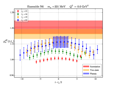
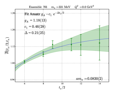
In the left panel of Fig. 1, results for the axial charge on the N6 ensemble are shown, where the effective axial charge is computed for four source-sink separations ranging from fm to fm. The symmetric approach to the central plateau region can clearly be seen. The data also exhibit a discrepancy between the midpoint values reached at different source-sink separations, indicating that excited-state contaminations are still present even when the ratio has apparently reached a plateau. To investigate the excited-state contribution in the plateau region further, the dataset was expanded to include source-sink separations of fm and fm. The right panel of Fig. 1 shows the results from applying a plateau fit to the data at 333For source-sink separations that are odd in lattice units, plateaus are fitted at for different source-sink separations . The dependence of the fit results on can be seen clearly. While the large errors at the largest source-sink separations fm somewhat obscure the trend, it is clear that may be underestimated when using plateau fits, and we do not employ plateau fits in our further analysis. Also shown is a fit to the expected -dependence, taking the energy gap to the excited state as a free parameter. The fit results are compatible with the assumption of a dominant S-wave state, although the uncertainty on the fit parameters is too large to make a conclusive argument.
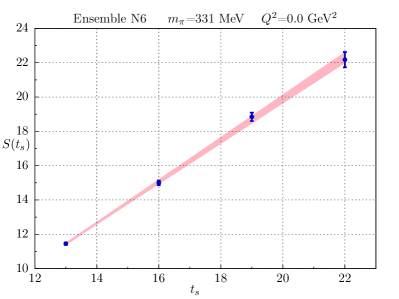
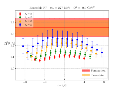
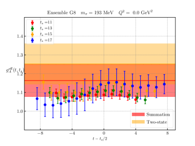
The results of various fit procedures are shown as coloured bands in the left panel of Fig. 1. The blue band indicates a plateau fit to source-sink separation fm, which is seen to lie significantly below the results of both of the analysis methods used in the following: the yellow band is a simultaneous fit to all source-sink separations and operator insertion times up to fm to the ansatz of Eq. (24), and the red band indicates the result obtained using the summation method. The quality of the linear fit performed in the latter method is illustrated in the bottom panel of Fig. 1. The results from the two-state fit and summation method agree very well with each other, indicating that residual excited-state effects are likely small on this ensemble. The effective axial charge on two of our most chiral ensembles is displayed in Fig. 2, together with the results of the summation and excited-state fits shown as bands. On ensemble F7, the two analysis methods are in very close agreement, while on G8 they differ in their result for by one standard deviation.
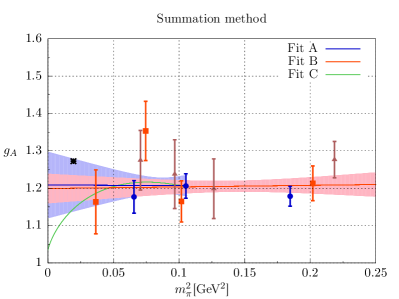
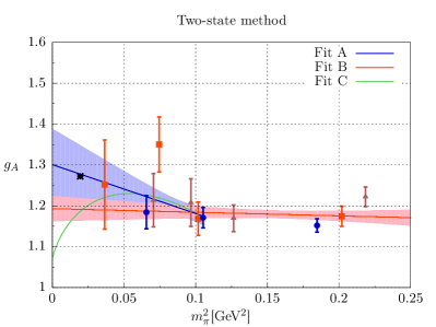
In Fig. 3, the results for obtained using the summation method (left panel) and two-state fits (right panel) on each of our ensembles are shown together with a chiral extrapolation to the physical pion mass. Details of the chiral extrapolation procedure will be presented in section VI. Here we note that the ensembles employed in our work all obey the constraint , and hence finite-volume effects are expected to be small. This is also supported empirically by our data, which do not display any noticeable volume dependence of . Similarly, no discernable dependence of on the lattice spacing is found in Fig. 3 for .
| Summation Method | Two-state Method | |||
| with | without | with | without | |
| 1 | 90.0 | n/a | 1.85 | n/a |
| 2 | 23.3 | 0.41 | 0.13 | 0.26 |
| 3 | 19.8 | n/a | 0.07 | n/a |
| 4 | 15.2 | n/a | 1.88 | n/a |
| 5 | 3.09 | 1.59 | 1.03 | 0.21 |
| 6 | 1.76 | 0.23 | 1.10 | 0.02 |
IV.2 Momentum-transfer dependence of the axial form factor
At non-zero momentum transfer, the determination of the axial form factor becomes more involved. In our choice of reference frame, the dependence of the effective form factors is no longer symmetric about the point ; as a consequence, we apply Eq. (22), as opposed to Eq. (24), when using the two-state fit method. Furthermore, both and contribute to the matrix elements and must be separated by solving the linear system of Eq. (19). As described above in section III, there are two ways in which the solution of the linear system can be combined with the analysis methods to account for excited-state contributions in order to extract the ground-state form factors, and we shall employ both of these in the following. Moreover, through the PCAC relation the matrix element of the pseudoscalar density provides an additional observable that can be used in conjunction with the matrix elements of the components of the axial current in order to determine the axial-current form factors. In the case of the axial form factor, we find that the determination of the form factor is relatively stable against the inclusion and exclusion of the pseudoscalar density in our basis of operators.
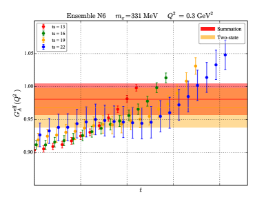
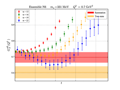
The results of evaluating the effective axial form factor on the N6 ensemble at the four-momentum transfers of GeV2 and GeV2 are shown in Fig. 4. At GeV2, which is the lowest non-vanishing four-momentum transfer that can be realised on this ensemble, no clear plateau appears for source-sink separations in the range of fm, and for the largest source-sink separation fm, the size of the uncertainties on the data make it difficult to decide whether a plateau has truly been reached.
Also shown are bands indicating the results of fitting the effective form factor using a two-state fit (Eq. (22)) and the summation method (Eq. (21)), and it can be seen that these agree with each other within their respective uncertainties. At the larger four-momentum transfer of GeV2, on the other hand, the results for the effective form factor at different source-sink separations show a clear downward trend in the central region, , where excited state contributions are expected to be most strongly suppressed, indicating that the plateau has not stabilized for fm. Furthermore, the results for obtained using the summation method and two-state fits are not in agreement with each other, which may be due to the more statistically precise data at the lower source-sink separations having a disproportionately strong influence on the fit results. This may introduce a bias in the two-state fit, but is likely to affect the slope of the summed ratio in the summation method even more. We will return to considering the relative reliability of the two methods when discussing the induced pseudoscalar form factor.
To confirm the stability of our analysis, we have verified that we obtain the same results for the axial form factor at each four-momentum transfer when we fit to the asymptotic behaviour of the effective form factors, and when we first extract the asymptotic behaviour of the ratios before isolating the form factors (i.e. methods 1 and 2 of section III yield consistent results). The values of obtained when solving the linear system of Eq. (19) after extracting asymptotic ratios using the summation method or two-state fits are shown in Table 2. The values of obtained with the summation method are large when is included. Nevertheless the results for the axial form factor are quite stable, regardless of whether the pseudoscalar density is excluded or included in the analysis. This may be attributed largely to the fact that the inclusion of affects the results for the induced pseudoscalar form factor much more strongly than those for ; we will further remark on this when discussing the induced pseudoscalar form factor in section V. When extracting the asymptotic ratios using two-state fits, the values of for Eq. (19) are rather reasonable both when including and when excluding the pseudoscalar density, and the results for (and for , as discussed in section V) are likewise compatible.
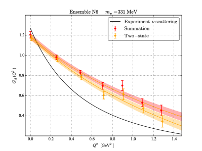
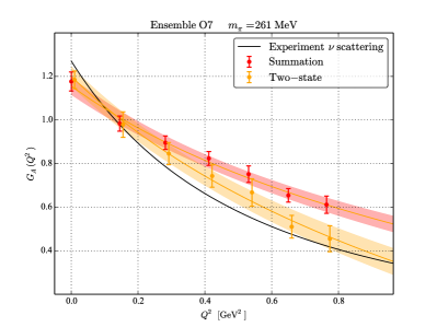
The momentum-transfer dependence of the axial form factor is shown in Fig. 5 for the ensembles N6 ( MeV) and O7 ( MeV). We note that while the results from the summation method and from two-state fits agree well near , the disagreement between them becomes larger with increasing , where the two-state fits tend to approach more closely the shape of the form factor inferred from experimental results, and this trend becomes more pronounced as the pion mass is decreased towards the physical point. We also note that (as previously observed elsewhereYamazaki:2008py ; Green:2012ud ; Capitani:2012gj ; Horsley:2013ayv ; Bhattacharya:2013ehc ; Bali:2014nma ; Chambers:2014qaa ; Bhattacharya:2016zcn ; Bouchard:2016heu ; Yoon:2016jzj ; Liang:2016fgy ; Berkowitz:2017gql ) while the lattice calculations tend to underestimate the axial charge, they tend to overestimate the value of the form factor at non-vanishing four-momentum transfer, leading to an underestimation of the axial radius of the nucleon.
IV.3 Model-independent determination of
While the momentum-transfer dependence of the axial form factor is frequently modelled with a dipole fit Bernard:2001rs , this leads to a model-dependence of the determination of the axial charge radius . Moreover, the use of the momentum transfer as the expansion variable has been shown to have a small radius of convergence, and the use of a conformally mapped parameter has been suggested Hill:2010yb ; Bhattacharya:2011ah in order to improve the convergence by parameterising the form factor in a model-independent manner as a power series in . The definition of and the corresponding power series for the form factor are given by
| (25) |
where is the three-pion kinematic threshold in the iso-vector axial-current channel. The power-series expansion of the form factor shown in Eq. (25) provides a controlled way of obtaining observables such as the axial radius in a model-independent fashion: once the coefficients have been determined from a fit to Eq. (25), the axial radius as defined in Eq. (4) can be derived from them in a straightforward manner.
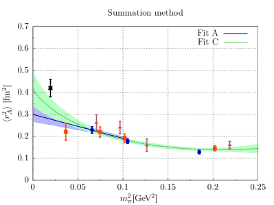
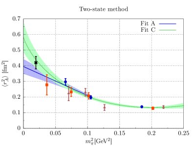
In this work, we have studied up to orders in the -expansion of Eq. (25), and the results at different orders were found to be consistent, provided that Bayesian priors were used to stabilize the fit; otherwise, the fits beyond became too unstable. While we have checked that the results for the axial charge radius obtained from the -expansion were stable against variations of the priors, we quote only the results obtained using the first order of the -expansion, where no priors were applied. The results obtained for the axial charge radius on our set of ensembles using the summation method and two-state fits are given in Tab. 17 and presented in Fig. 6 together with a chiral extrapolation to the physical pion mass. For details of the chiral extrapolation, the reader is referred to section VI. For now, we make the qualitative observation that the mean-square radius increases by roughly a factor two between and . Similar to the axial charge, no systematic trend of the axial radius as a function fo the lattice spacing is seen.
V Isovector induced pseudoscalar form factor
The momentum transfer dependence of the induced pseudoscalar form factor is markedly different from that of the axial form factor due to the presence of a pole at the pion mass arising as a consequence of chiral symmetry breaking. The low-momentum behaviour of may therefore be expected to be rather steep, with possibly considerable statistical fluctuations in the low- region. In this section, we discuss the determination of the induced pseudoscalar form factor from our various analysis methods for suppressing excited-state contributions, and how these are affected by the choice of either including or excluding the pseudoscalar density in our operator basis.
Relation (9) expresses the PCAC relation at the level of ground-state matrix elements. Since the extraction of the latter from the three-point function comes with an additional uncertainty due to potential contamination from excited states, we initially test the PCAC relation at the correlator level,
| (26) | |||
We have checked that the left-hand side has an average compatible with zero. For instance, on ensemble O7 at the smallest available spatial momentum, the absolute statistical uncertainty on the left-hand side is no more than 0.01 for all values of and HuaThesis . Thus the violation of the PCAC relation due to discretization errors appears to be small. Therefore, we adopt the point of view that the consistency condition (9) on the ground-state matrix elements can be used as a way to test the ability of the summation method and the two-state fits to extract the ground-state matrix elements.
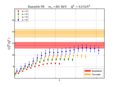
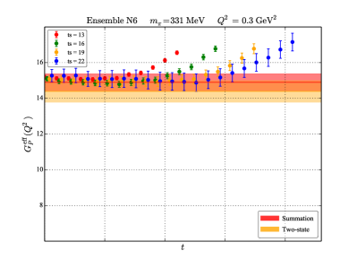
In order to gain insight into the nature of the excited-state contributions, we first construct the effective form factor by solving the linear system of Eq. (19) at each four-momentum , operator insertion time , and source-sink separation . In doing so, we find a marked difference in the time-separation dependence of between the case where only components of the axial current are included in solving Eq. (19) and the case where a combination of components of the axial current as well as pseudoscalar density are included. This is in contrast to the situation for the axial form factor , where no strong dependence on the inclusion or exclusion of in the operator basis was observed. The results for both cases are shown in Fig. 7. It can be clearly seen that the choice of whether to include the pseudoscalar density has a significant and non-trivial impact on the time-dependence of the effective induced pseudoscalar form factor. For the case where only the axial current is included in the determination (shown in the left panel of Fig. 7), the results asymptote from below, with much stronger excited-state effects visible at the source as compared to the sink. The apparent plateaux reached at different source-sink separations do not agree with each other, indicating that the contribution from excited states is substantial at time separations as large as fm. For the case where both the pseudoscalar density and the axial current are included in the determination (shown in the right panel of Fig. 7), the results are much less time-dependent and asymptote from above, with stronger excited-state effects seen at the sink rather than the source. The plateaux for different source-sink separations agree with each other within their respective statistical uncertainties. However, the plateau values differ significantly from those seen when excluding , even at the largest source-sink separations, which further indicates that excited-state contamination remains a significant effect even at fm.
Also shown in Fig. 7 are the results of applying each of our excited-state analysis methods, viz. the summation method (red bands) and two-state fits (yellow bands). It can be seen that when extracting the induced pseudoscalar form factor using only the axial current, the results from the two methods disagree significantly, which may indicate that excited-state effects are not under control. When including the pseudoscalar density in the determination, on the other hand, the results from the summation and two-state methods agree within their respective error bands. As pointed out in section IV, the matrix elements of the pseudoscalar density are found to be statistically more precise in comparison to those of the axial current, and hence strongly influence the determination of the effective form factors. Their impact on the results seems to be limited to the induced pseudoscalar form factor, however. Judging both from the appearance of the effective form factor and from the agreement between our analysis methods, the excited-state effects seem to be smaller in the case where the pseudoscalar density is included. We conclude that its inclusion is beneficial and therefore keep the pseudoscalar density as part of all subsequent analyses.
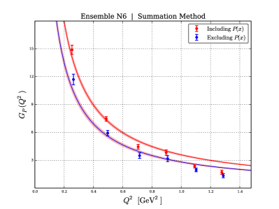
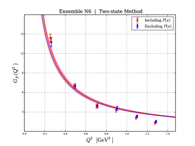
The dependence on of the results obtained using each of our analysis methods when including or excluding the pseudoscalar density in the solution of Eq. (19) is presented in Fig. 8. The form factors obtained with the summation method (shown in the left panel of Fig. 8) can be seen to be particularly sensitive to the inclusion of the pseudoscalar density, with a clear gap opening up particularly in the low- regime. This is also evident from the large values of for the solution of Eq. (19) shown in the relevant columns of Table 2 and may indicate that the summation method is not able to properly account for the large excited-state contamination found in when using only the axial current. By contrast, the results obtained using the two-state method (shown in the right panel of Fig. 8) indicate good stability against the choice of including or excluding the pseudoscalar density. This observation is corroborated by the values of shown in the relevant columns of Table 2. It is also worth noting that while the results from the summation method show a high sensitivity to the choice of the operator basis used in solving Eq. (19), a marked improvement in the compatibility with the results from the two-state method is observed when the pseudoscalar density is included. Since judging from their stability under the choice of operator basis, the results obtained with the two-state method appear to be more reliable, the two-state method will be the method of choice in our subsequent analysis.
In summary, the ground-state matrix elements extracted with the two-state fit method are overall consistent with the PCAC relation Eq. (9), which is a non-trivial check that excited-state contaminations have been removed, since the extraction of each term in Eq. (9) may be affected differently by excited states. By contrast, the ground-state matrix elements extracted with the summation method do not satisfy the PCAC relation, as seen from the large reduced values in Table 2; we therefore do not use the summation method for our final results, but nonetheless quote intermediate results derived from it in tables 4 and 5. In the future, we hope to carry out high-statistics calculations at such large source-sink separations that both methods yield ground-state matrix elements that are consistent with each other and with the PCAC relation.
VI Chiral Analysis
In order to provide predictions for the physical world, it remains to extrapolate our lattice results obtained at unphysical values of the light quark masses to the physical pion mass and the continuum limit. The standard approach to this problem is to take the values of the observables of interest ( and the axial charge radius in our case) as determined on each ensemble, and to extrapolate them to the physical point using formulae taken from, or inspired by, Chiral Perturbation Theory (ChPT).
VI.1 Combined fit in chiral effective theory
| Interaction | Low-energy constant | Value and role in the fit |
| MeV | ||
| Lattice input | ||
| GeV (Ref. Olive:2016xmw ) | ||
| Fit parameter contributing to and | ||
| Lattice input | ||
| or MeV | ||
| Fit parameter contributing to and | ||
| (Ref. Becher:2001hv ) | ||
| or GeV-1 (Refs. Hoferichter:2015hva ; Hoferichter:2015tha ) | ||
| (Ref. Becher:2001hv ) | ||
| or GeV-1 (Refs. Hoferichter:2015hva ; Hoferichter:2015tha ) | ||
| Fit parameter contributing to and | ||
| Fit parameter contributing to | ||
| Fit parameter contributing to and |
One possible approach that can be applied here is very similar to that performed in our paper Capitani:2015sba on the electromagnetic form factors of the nucleon: we perform a fit of the dependence of the form factors and on both the pion mass and the squared momentum transfer to the expressions of baryonic effective field theory (EFT), including explicit axial vector degrees of freedom Schindler:2006it . The main motivation for this ansatz is that the inclusion of the axial vector meson extends the range in for which a phenomenologically good description of the form factor data is achieved Schindler:2006it . This increases the number of points amenable to a simultaneous fit to the and pion mass dependence of the form factors and . From such a fit we extract the LECs and subsequently use the so obtained values at the physical pion mass to quote the extrapolated result for our data. This approach avoids the two-step procedure of first extracting the form factors and derived quantitites using a dipole fit or a -expansion analysis, before applying a chiral extrapolation. It also has the potential advantage that values are obtained for low-energy constants that can be used in describing other obervables.
The full analytic form of the ansatz is quite lengthy; it can be found in Schindler:2006it . While we do not reproduce it in its full length here, the contributions of the fit parameters to and are simple to write down,
| (27) | |||||
| (28) | |||||
where indicates terms of at least one-loop order. The fitted low-energy constants are , , , and , as summarized in Table 3. The low-energy constants and , and the mass of the axial vector meson are set to their phenomenological values Becher:2001hv , while for the nucleon mass its measured value on each ensemble is used. A pion-mass cut of MeV is applied to the fits, which thereby only include four ensembles, as well as a momentum cut of GeV2. The reason for the reduction in the fit range is that we obtained values for the of about 4-5 with the less restrictive choice of MeV made in the next subsection. We perform a simultaneous fit to both and using a fit function accounting for the leading discretisation effects,
| (29) |
In order to estimate the influence of various systematic effects, we also perform a number of variations on the fit by
-
1.
neglecting discretisation effects (),
-
2.
not applying a cut in ,
-
3.
using the physical nucleon mass on all ensembles, and
-
4.
using different values for the low-energy constants and .
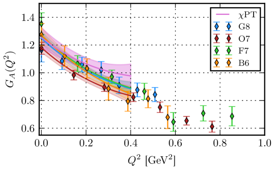
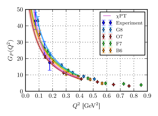
Examples of the standard fit are shown in figures 9 and 10, and the values for , , and resulting at the physical pion mass for the different variations are tabulated in Table 4. The shape and overall normalization of in particular compares very favourably with the (limited) experimental data. The axial charge in the chiral limit tends to come out at a large value, while the obtained value of the parameter gives an unnaturally large negative slope of as a function of . For this and other reasons given in section VII, we use fits to the pion-mass dependence of the axial charge and radius for our final results; these fits are presented in the next subsection. Nonetheless, we think that the effectiveness and stability of the EFT fit should be re-evaluated once more accurate data at small pion mass and virtualities becomes available.
| Fit variant | Method | [fm2] | ||||
|---|---|---|---|---|---|---|
| Standard | summation | 1.255(71) | 0.238(77) | 8.3(5) | 0.59 | 19 |
| No | 1.318(41) | 0.216(58) | 8.8(3) | 0.63 | 23 | |
| No cut | 1.325(48) | 0.217(29) | 8.8(3) | 0.61 | 43 | |
| With | 1.314(78) | 0.217(75) | 8.9(5) | 1.71 | 19 | |
| Alternative | 1.336(71) | 0.209(73) | 8.8(5) | 0.47 | 19 | |
| Standard | two-state | 1.382(91) | 0.246(92) | 9.0(7) | 0.50 | 19 |
| No | 1.418(66) | 0.202(69) | 9.4(4) | 0.61 | 23 | |
| No cut | 1.427(70) | 0.287(36) | 9.4(5) | 0.50 | 43 | |
| With | 1.399(98) | 0.214(92) | 9.4(7) | 1.25 | 19 | |
| Alternative | 1.478(91) | 0.222(86) | 9.7(7) | 0.29 | 19 |
VI.2 HBChPT-inspired fits
In order to enable a comparison with the standard approach, we also perform fits to the pion-mass dependence of the axial radius and the axial charge using several variants of HBChPT-inspired chiral fits. In order to determine whether our data allow for the resolution of the chiral logarithm, we fit each quantity using the ansätze
| (30) | ||||
| (31) |
with three and two fit parameters, respectively. The linear fit (30) is applied both with (Fit A) and without (Fit B) a pion-mass cut of MeV444The ensemble N6 is included both in Fit A and in Fit B. in order to check for the importance of higher-order corrections, while the fit (31) including a logarithmic term is applied over the whole pion mass range (Fit C).
In the case of the axial charge, we use a modified version of Fit C, namely
| (32) |
with fit parameters and , and the chiral-limit pion decay constant fixed to its phenomenological value MeV Colangelo:2003hf ; Aoki:2016frl ; a pion-mass cut of MeV is applied in this case. The reason is that using Eq. (31) with the coefficient of the logarithmic term left free gives implausible results in that the sign of the logarithmic term comes out positive, contrary to the ChPT result incorporated into Eq. (32). Comparing the results of the different fits (cf. Fig. 3), we conclude that our data are not precise enough to allow for a reliable resolution of the chiral logarithm, and that applying the fit form 32 amounts to imposing a trend which is not seen at all in our data. Even with Fit A, we observe that the slope of as a function of is only poorly constrained. In the results presented in Table 5, we have assumed that the results are independent of the lattice spacing, since we already observed that no particular trend in the cutoff dependence is seen in the or data for MeV. For an indication of how sensitive the results are to this assumption, we quote the result of a simultaneous linear extrapolation in and (i.e. a three-parameter fit) of the axial charge for MeV: we find at the physical pion mass, to be compared with assuming no cutoff effects. The difference is well contained in the uncertainty estimate. At the same time, we note that the description including O() cutoff effects is overfitting the data, as witnessed by the fact that the goes up from 1.07 to 1.21 in spite of the additional fit parameter. As a further alternative, if we perform Fit A without an O( but remove the data from the coarsest lattice spacing, we obtain at the physical pion mass, i.e. no change except for an insignificant increase in the statistical uncertainty.
| [fm2] | |||
|---|---|---|---|
| Two-state fit | |||
| Fit A | 1.278(68) | 0.360(36) | 7.7(1.8) |
| Fit B | 1.191(27) | 0.271(12) | 8.5(1.5) |
| Fit C | 1.186(56) | 0.440(47) | 5.7(2.1) |
| Summation method | |||
| Fit A | 1.208(69) | 0.279(26) | 8.2(1.6) |
| Fit B | 1.200(34) | 0.242(12) | 8.0(1.5) |
| Fit C | 1.138(59) | 0.330(39) | 7.6(1.9) |
For the axial charge radius, we find that the linear fits without a pion-mass cut do not describe our data well, whereas both the linear fits with a pion-mass cut and the fits including a logarithmic term are well compatible with our data (cf. Fig. 6).
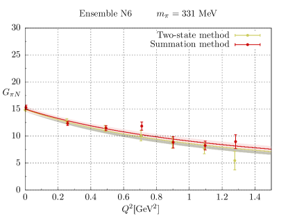
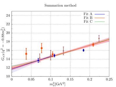
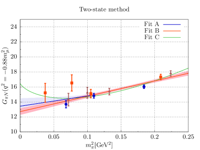
The pseudoscalar coupling defined by Eq. (5) is not readily accessible from our results for because its and dependence is strong, due to the pion pole. However, observing that the pion-nucleon form factor depends less strongly on and , we proceed as follows. First, the form factor is determined on every ensemble at the available values by taking the appropriate linear combination of and ; see Eqs. (8) and (9). Then a monopole fit is performed (see Fig. 11),
| (33) |
which allows us to extract on every ensemble. The latter is then chirally (and continuum) extrapolated to the physical point; see Fig. 12. We use the already determined values of and at the physical pion mass to obtain via (3), since is very small. Finally, taking the appropriate linear combination of and yields at the physical pion mass. The momentum-transfer dependence (33) of was proposed in Schindler:2006it ; it describes the lattice data well, as can be seen from Fig. 11. We find that this dependence is very mild, reflecting the fact that the pion pole describes the bulk of the dependence of . Since is small on hadronic scales and Eq. 9 implies , the sensitivity of to the specific form of the ansatz (33) is weak.
A summary of our results for , , and can be found in Table 5.
VII Discussion and Conclusion
As discussed above, we use in our main analysis the form factors extracted with the two-state fit in order to remove excited-state contributions. We include the pseudoscalar density in our analysis, as its matrix elements are overall compatible with those of the axial current via the PCAC relation and tend to increase the precision of the calculation.
As for the chiral extrapolation, we have performed simultaneous fits to the pion-mass and momentum transfer dependence, as well as the more widely used two-step procedure of first extracting the small- observables and then chirally extrapolating them. A disadvantage of the simultaneous chiral fits to and is that it is intrinsically a small- expansion, and the paucity of the lattice data in this region, as compared to previous lattice calculations of the pion electromagnetic form factor Brandt:2013dua , adversely affects the stability of the fits. Empirically, we find that the fitted values of the low-energy constants and come out large and poorly constrained, casting some doubt on whether convergence is under control. Secondly, in the chiral expansion the leading correction to the (pion-mass independent) leading-order value for the slope of the axial form factor happens to vanish; this implies that the fit ansatz imposes a pion-mass dependence of the axial radius which is completely dominated by the pion-mass dependence of the axial charge (see Eq. (4)). Third, the chiral logarithm predicted in the pion-mass dependence of the axial charge is not seen in the data (see Fig. 3). For these reasons, unlike in our study of the vector form factors Capitani:2015sba , we prefer in the present study to quote as final results those obtained with the more conventional procedure of first extracting the axial charge and radius and on each ensemble, followed by a chiral extrapolation. Nonetheless, we have presented the effective field theory analysis because this type of combined fits may be useful in future calculations involving more accurate data in the very chiral and low-momentum regime.
For our final numbers, we choose to quote the result of applying a linear fit with a pion-mass cut of MeV (Fit A) to the data obtained from the two-state fit method. We estimate the systematic error from the chiral extrapolation by taking the difference between the fits with and without a pion-mass cut (Fits A and B) as a one-sided systematic error; where the fit including a logarithmic term (Fit C) lies on the other side of our central value, we include the corresponding difference into an asymmetric two-sided systematic error. We note that the results from the summation method are also covered by the resulting error bars, and that our results are therefore not sensitive to excited-state effects at this level of accuracy. We thus finally obtain
| (34) | |||||
where the first error is statistical and the second systematic. All three results are compatible with the phenomenological values of these quantities: (the Particle Data Group average of neutron decay data Olive:2016xmw ), (from a dipole fit to neutrino scattering data, see Bernard:2001rs for a review and other determinations of the axial charge radius), and (from the MuCap experiment Andreev:2012fj ; Andreev:2015evt ).
Several other lattice calculations of the axial charge have appeared recently Bali:2014nma ; Abdel-Rehim:2015owa ; Bhattacharya:2016zcn ; Yoon:2016jzj ; Berkowitz:2017gql ; Meyer:2016kwb ; Alexandrou:2017msl ; Green:2017keo ; Alexandrou:2017hac ; Rajan:2017lxk . In particular, the values obtained in Bali:2014nma ; Abdel-Rehim:2015owa ; Bhattacharya:2016zcn ; Yoon:2016jzj ; Berkowitz:2017gql at the physical pion mass also agree with the phenomenological value, while the calculation in Alexandrou:2017hac yields a slightly lower value. Most of them quote a rather more precise result, however the precision depends strongly on the source-sink separations and the ranges of pion masses used in the chiral extrapolation. For example, as compared to our earlier publication on the axial charge Capitani:2012gj , the final quoted error has changed little, but the present chiral extrapolation is based on the interval , rather than on . This comparison also illustrates the increasing computational cost of determining nucleon structure observables as the pion mass is reduced.
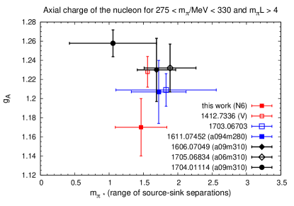
In order to remove the effect of applying different procedures for the chiral extrapolations, in Fig. 13 we compare recent lattice results for the axial charge at MeV obtained on reasonably large and fine lattices satisfying and fm. Since the range of source-sink separations used in the calculations is one of the main quality criteria, we indicate this range by a horizontal segment in Fig. 13. Within the uncertainties of the comparison, we observe a consistent picture. Most results cluster between 1.20 and 1.24, while the central value of our result on ensemble N6 lies somewhat lower. While the available data does not allow one to identify a specific trend as a function of the flavor content of the calculations or on the lattice spacing, future continuum-extrapolated results would allow for a more controlled comparison. Finally, we remark that the challenge for the future will be to maintain or improve the statistical precision while extracting the axial charge exclusively from source-sink separations exceeding 1.5 fm.
To a more limited extent, we can also compare our result for the axial radius to other lattice determinations. Again, we favor performing the comparison at a fixed pion mass of about 300 MeV. In extracting the radius, the precise fit form used to describe the axial form factor plays an important role, both for the central value and the achieved statistical precision. Using a dipole fit, Ref. Rajan:2017lxk obtains for on their ensemble a06m310; with a dipole fit, our result for on ensemble N6 agrees very well. Also, at Ref. Green:2017keo obtains , where we have added the errors in quadrature, from a -expansion fit with five terms and Gaussian priors starting at the third term. These recent results are thus in good agreement.
Probably the most critical step in the presented lattice calculation is the extraction of the ground-state matrix elements from the correlation functions. We have used two theoretically well motivated methods, the summation and two-state method described in section III, in order to perform this task. For the axial form factor at , we observe good agreement between the two methods, adding confidence in the results for and . The situation for the form factors containing the pion pole (, ) is less satisfactory, in the sense that only the two-state-fit method led to ground-state matrix elements consistent with the PCAC relation Eq. (9). It is for that reason that we chose the two-state-fit method to present our final results. In the future, by performing calculations at larger source-sink separations, we hope to benefit from more cross-checks, as in the case of the axial form factor. At the same time, the corrections to the mid-point values of the ratios , induced by the summation or two-state-fit method in extracting the ground-state matrix elements, would be reduced.
In summary, we have performed a two-flavour lattice QCD calculation of the isovector axial and induced pseudoscalar nucleon form factors. We have consistently applied the improvement program and observe no significant cutoff effect on the low- observables at pion masses below 350 MeV. We have made use of the pseudoscalar density. Its form factor is related to the axial and induced pseudoscalar form factor by the PCAC relation, and thus it provides both a cross-check of the calculation and a slight increase in precision. The axial charge, the axial radius and the pseudoscalar coupling we obtained are in agreement with experiment.
In the near future, we plan to improve on our calculation by using -flavour ensembles (i.e. containing the sea-quark effects of both the light and strange quarks), by increasing the statistics by an order of magnitude and by going to larger source-sink separations. A preliminary account of the results was presented at the Lattice 2016 conference Djukanovic:2016ocj . The lessons learnt from the analysis applied here will be beneficial in this endeavour.
Acknowledgments
We are grateful to our colleagues within the CLS initiative for sharing ensembles. We have used the LoopTools library Hahn:1998yk in the numerical evaluation of the EFT amplitudes Schindler:2006it .
Our calculations were performed on the “Wilson” HPC Cluster at the Institute for Nuclear Physics, University of Mainz, and on the “Clover” HPC Cluster at the Helmholtz Institute Mainz. We are grateful to Christian Seiwerth for technical support. We are also grateful for computer time allocated to project HMZ21 on the BG/Q “JUQUEEN” computer at NIC, Jülich. This work was granted access to the HPC resources of the Gauss Center for Supercomputing at Forschungzentrum Jülich, Germany, made available within the Distributed European Computing Initiative by the PRACE-2IP, receiving funding from the European Community’s Seventh Framework Programme (FP7/2007-2013) under Grant No. RI-283493.
This work was supported by the Deutsche Forschungsgemeinschaft (DFG) in the SFB 443 and SFB 1044, and by the Rhineland-Palatinate Research Initiative. M.D.M. was partially supported by the Danish National Research Foundation under Grant No. DNRF:90. B.J. was supported by the Schweizerischer Nationalfonds (SNF) under grant 200020-162515. P.M.J. acknowledges support from the Department of Theoretical Physics, TIFR. T.D.R. was supported by DFG grant HA4470/3-1.
Appendix A Form factor values
In Tables 6–16 we give all of our results for the iso-vector axial form factors and of the nucleon at all values of measured on each ensemble. Listed in each case are the values obtained using the summation method and an explicit two-state fit (cf. the main text for details). The statistical errors on each data point are quoted in parentheses following the central value.
| A3 | ||||||
|---|---|---|---|---|---|---|
| [] | Two-state | Summation | Two-state | Summation | Two-state | Summation |
| 0.0 | 1.222 (0.024) | 1.276 (0.049) | - | - | 18.03 (0.356) | 18.83 (0.717) |
| 0.230 | 1.057 (0.025) | 1.052 (0.041) | 17.47 (0.664) | 16.88 (1.125) | 15.43 (0.413) | 15.84 (0.637) |
| 0.448 | 0.922 (0.026) | 0.919 (0.040) | 9.829 (0.345) | 10.14 (0.568) | 14.63 (0.598) | 13.68 (0.805) |
| 0.655 | 0.790 (0.033) | 0.755 (0.054) | 6.222 (0.338) | 6.034 (0.575) | 14.04 (0.833) | 12.99 (1.313) |
| 0.823 | 0.680 (0.043) | 0.597 (0.074) | 4.656 (0.381) | 4.057 (0.678) | 11.37 (1.011) | 10.27 (1.812) |
| 1.013 | 0.675 (0.051) | 0.612 (0.084) | 3.955 (0.323) | 3.722 (0.561) | 11.13 (1.080) | 8.616 (1.793) |
| 1.196 | 0.585 (0.067) | 0.494 (0.115) | 2.858 (0.357) | 2.466 (0.649) | 11.75 (1.694) | 9.133 (2.869) |
| A4 | ||||||
|---|---|---|---|---|---|---|
| [] | Two-state | Summation | Two-state | Summation | Two-state | Summation |
| 0.0 | 1.170 (0.033) | 1.199 (0.080) | - | - | 15.42 (0.430) | 15.80 (1.054) |
| 0.229 | 1.022 (0.038) | 0.985 (0.042) | 16.41 (1.069) | 15.74 (1.135) | 14.04 (0.826) | 13.64 (0.914) |
| 0.442 | 0.978 (0.054) | 0.984 (0.074) | 9.304 (0.541) | 9.258 (0.771) | 16.35 (2.337) | 16.90 (2.163) |
| 0.643 | 0.823 (0.056) | 0.817 (0.074) | 6.064 (0.492) | 5.812 (0.670) | 12.92 (1.242) | 14.51 (2.047) |
| 0.805 | 0.926 (0.164) | 0.822 (0.161) | 6.017 (1.184) | 5.299 (1.133) | 10.39 (1.894) | 9.725 (2.688) |
| 0.987 | 0.674 (0.088) | 0.546 (0.103) | 3.429 (0.486) | 2.857 (0.584) | 11.63 (1.648) | 7.992 (2.287) |
| 1.162 | 0.575 (0.106) | 0.359 (0.159) | 2.537 (0.509) | 1.830 (0.712) | 10.18 (1.893) | 0.205 (4.267) |
| A5 | ||||||
|---|---|---|---|---|---|---|
| [] | Two-state | Summation | Two-state | Summation | Two-state | Summation |
| 0.0 | 1.208 (0.058) | 1.238 (0.092) | - | - | 15.27 (0.738) | 15.65 (1.165) |
| 0.228 | 1.018 (0.069) | 0.987 (0.064) | 16.96 (1.541) | 16.90 (1.462) | 12.88 (0.941) | 11.72 (1.003) |
| 0.440 | 0.853 (0.072) | 0.869 (0.078) | 8.433 (0.822) | 8.662 (0.934) | 11.94 (1.111) | 11.74 (1.056) |
| 0.638 | 0.620 (0.088) | 0.642 (0.099) | 4.386 (0.739) | 4.245 (0.816) | 10.13 (1.910) | 13.71 (2.561) |
| 0.797 | 0.451 (0.143) | 0.424 (0.162) | 2.343 (0.946) | 2.067 (1.105) | 12.45 (2.555) | 13.94 (3.250) |
| 0.977 | 0.410 (0.094) | 0.357 (0.115) | 2.075 (0.485) | 1.775 (0.616) | 5.331 (2.239) | 5.396 (2.410) |
| 1.148 | 0.389 (0.149) | 0.376 (0.187) | 1.731 (0.641) | 1.451 (0.813) | 4.088 (5.517) | 11.20 (5.863) |
| B6 | ||||||
|---|---|---|---|---|---|---|
| [] | Two-state | Summation | Two-state | Summation | Two-state | Summation |
| 0.0 | 1.214 (0.065) | 1.275 (0.080) | - | - | 14.56 (0.781) | 15.29 (0.957) |
| 0.104 | 1.158 (0.095) | 1.120 (0.074) | 35.15 (3.090) | 34.82 (2.519) | 12.16 (1.285) | 11.26 (0.986) |
| 0.204 | 1.053 (0.094) | 1.031 (0.069) | 18.38 (1.807) | 18.06 (1.322) | 13.36 (1.441) | 12.99 (1.084) |
| 0.301 | 0.894 (0.112) | 0.886 (0.082) | 11.44 (1.549) | 10.78 (1.173) | 12.14 (2.959) | 14.13 (1.857) |
| 0.387 | 0.830 (0.096) | 0.794 (0.072) | 9.049 (1.142) | 8.792 (0.898) | 9.013 (1.865) | 7.812 (1.537) |
| 0.478 | 0.877 (0.092) | 0.812 (0.065) | 7.807 (0.833) | 7.222 (0.614) | 10.87 (2.163) | 10.16 (1.061) |
| 0.566 | 0.743 (0.119) | 0.679 (0.082) | 5.606 (0.843) | 4.837 (0.671) | 10.44 (5.042) | 13.06 (2.402) |
| E5 | ||||||
|---|---|---|---|---|---|---|
| [] | Two-state | Summation | Two-state | Summation | Two-state | Summation |
| 0.0 | 1.174 (0.025) | 1.213 (0.047) | - | - | 17.54 (0.368) | 18.12 (0.695) |
| 0.357 | 0.958 (0.026) | 0.971 (0.038) | 12.85 (0.521) | 13.11 (0.752) | 14.47 (0.480) | 14.52 (0.686) |
| 0.685 | 0.741 (0.028) | 0.727 (0.040) | 5.680 (0.290) | 5.434 (0.419) | 14.76 (0.615) | 15.28 (0.849) |
| 0.991 | 0.621 (0.041) | 0.560 (0.065) | 3.644 (0.307) | 3.102 (0.486) | 12.67 (0.968) | 13.47 (1.596) |
| 1.236 | 0.575 (0.057) | 0.535 (0.099) | 2.816 (0.317) | 2.620 (0.566) | 12.27 (1.434) | 11.45 (2.540) |
| 1.511 | 0.491 (0.053) | 0.413 (0.090) | 2.064 (0.238) | 1.676 (0.411) | 10.08 (1.264) | 9.950 (2.194) |
| 1.772 | 0.455 (0.071) | 0.397 (0.130) | 1.627 (0.275) | 1.390 (0.504) | 10.93 (1.975) | 10.48 (3.452) |
| F6 | ||||||
|---|---|---|---|---|---|---|
| [] | Two-state | Summation | Two-state | Summation | Two-state | Summation |
| 0.0 | 1.169 (0.041) | 1.165 (0.055) | - | - | 15.12 (0.529) | 15.07 (0.712) |
| 0.163 | 1.034 (0.059) | 1.014 (0.048) | 21.60 (1.655) | 21.69 (1.397) | 13.88 (0.667) | 13.15 (0.577) |
| 0.317 | 0.887 (0.052) | 0.886 (0.045) | 11.23 (0.754) | 11.02 (0.676) | 13.81 (0.842) | 14.37 (0.660) |
| 0.464 | 0.781 (0.062) | 0.801 (0.056) | 7.279 (0.694) | 6.993 (0.599) | 13.41 (1.128) | 16.45 (1.159) |
| 0.595 | 0.677 (0.069) | 0.690 (0.066) | 5.124 (0.663) | 5.297 (0.661) | 12.42 (1.016) | 12.02 (1.061) |
| 0.731 | 0.598 (0.058) | 0.653 (0.055) | 3.857 (0.423) | 4.217 (0.393) | 10.90 (0.953) | 11.79 (0.932) |
| 0.862 | 0.556 (0.078) | 0.601 (0.076) | 3.118 (0.494) | 3.331 (0.479) | 10.35 (1.070) | 11.94 (1.265) |
| F7 | ||||||
|---|---|---|---|---|---|---|
| [] | Two-state | Summation | Two-state | Summation | Two-state | Summation |
| 0.0 | 1.350 (0.067) | 1.353 (0.079) | - | - | 16.79 (0.838) | 16.83 (0.986) |
| 0.162 | 1.112 (0.082) | 1.066 (0.058) | 23.86 (2.205) | 24.10 (1.577) | 14.70 (1.218) | 12.63 (0.893) |
| 0.315 | 0.991 (0.069) | 0.971 (0.048) | 13.12 (1.015) | 12.78 (0.704) | 13.21 (1.585) | 13.21 (1.020) |
| 0.461 | 0.868 (0.080) | 0.866 (0.058) | 8.250 (0.855) | 7.930 (0.604) | 12.89 (2.908) | 15.16 (1.828) |
| 0.591 | 0.636 (0.093) | 0.645 (0.068) | 4.608 (0.828) | 4.857 (0.606) | 13.06 (2.159) | 11.03 (1.658) |
| 0.725 | 0.708 (0.077) | 0.707 (0.055) | 4.516 (0.516) | 4.535 (0.381) | 11.51 (1.953) | 11.10 (1.216) |
| 0.854 | 0.661 (0.099) | 0.686 (0.070) | 3.676 (0.576) | 3.845 (0.411) | 10.22 (2.981) | 9.864 (1.538) |
| G8 | ||||||
|---|---|---|---|---|---|---|
| [] | Two-state | Summation | Two-state | Summation | Two-state | Summation |
| 0.0 | 1.252 (0.109) | 1.163 (0.086) | - | - | 14.93 (1.302) | 13.87 (1.020) |
| 0.092 | 1.178 (0.136) | 1.085 (0.062) | 43.19 (6.346) | 43.00 (2.867) | 14.79 (1.464) | 11.11 (0.713) |
| 0.182 | 1.138 (0.119) | 1.059 (0.053) | 26.68 (2.547) | 22.61 (1.167) | 9.900 (2.976) | 15.01 (1.245) |
| 0.268 | 1.060 (0.133) | 1.021 (0.061) | 17.90 (2.238) | 15.87 (1.048) | 7.183 (3.578) | 14.26 (1.346) |
| 0.348 | 0.955 (0.130) | 0.909 (0.059) | 11.49 (1.760) | 11.36 (0.805) | 16.24 (1.973) | 11.72 (0.984) |
| 0.430 | 0.854 (0.109) | 0.876 (0.050) | 9.013 (1.155) | 9.068 (0.534) | 8.564 (1.891) | 11.20 (0.835) |
| 0.509 | 0.776 (0.113) | 0.843 (0.051) | 7.059 (1.048) | 7.449 (0.478) | 6.507 (2.159) | 11.07 (0.816) |
| N5 | ||||||
|---|---|---|---|---|---|---|
| [] | Two-state | Summation | Two-state | Summation | Two-state | Summation |
| 0.0 | 1.152 (0.016) | 1.179 (0.027) | - | - | 16.18 (0.230) | 16.55 (0.372) |
| 0.256 | 0.982 (0.020) | 0.992 (0.022) | 15.24 (0.459) | 15.42 (0.499) | 13.57 (0.331) | 13.66 (0.380) |
| 0.494 | 0.845 (0.018) | 0.874 (0.021) | 8.193 (0.207) | 8.513 (0.243) | 12.63 (0.418) | 12.96 (0.416) |
| 0.719 | 0.745 (0.024) | 0.796 (0.028) | 5.393 (0.197) | 5.608 (0.237) | 11.71 (0.668) | 13.62 (0.693) |
| 0.918 | 0.648 (0.035) | 0.682 (0.041) | 3.910 (0.237) | 4.091 (0.290) | 9.718 (0.696) | 10.53 (0.932) |
| 1.122 | 0.566 (0.031) | 0.614 (0.039) | 2.836 (0.164) | 3.113 (0.214) | 9.377 (0.644) | 9.622 (0.708) |
| 1.317 | 0.532 (0.038) | 0.582 (0.051) | 2.343 (0.169) | 2.538 (0.242) | 8.522 (1.113) | 9.934 (1.040) |
| N6 | ||||||
|---|---|---|---|---|---|---|
| [] | Two-state | Summation | Two-state | Summation | Two-state | Summation |
| 0.0 | 1.171 (0.025) | 1.206 (0.033) | - | - | 14.84 (0.317) | 15.29 (0.415) |
| 0.254 | 0.968 (0.030) | 0.981 (0.024) | 14.39 (0.612) | 14.90 (0.486) | 12.76 (0.444) | 12.32 (0.375) |
| 0.487 | 0.785 (0.027) | 0.827 (0.023) | 6.996 (0.288) | 7.459 (0.246) | 11.38 (0.565) | 11.45 (0.452) |
| 0.705 | 0.604 (0.037) | 0.697 (0.033) | 3.877 (0.284) | 4.454 (0.256) | 10.07 (0.961) | 11.83 (0.763) |
| 0.897 | 0.613 (0.054) | 0.700 (0.049) | 3.296 (0.315) | 3.827 (0.288) | 8.780 (1.040) | 8.824 (1.060) |
| 1.092 | 0.472 (0.043) | 0.530 (0.039) | 2.098 (0.202) | 2.367 (0.192) | 7.681 (0.975) | 8.233 (0.818) |
| 1.277 | 0.344 (0.056) | 0.453 (0.053) | 1.333 (0.220) | 1.708 (0.222) | 5.444 (1.721) | 8.951 (1.281) |
| O7 | ||||||
|---|---|---|---|---|---|---|
| [] | Two-state | Summation | Two-state | Summation | Two-state | Summation |
| 0.0 | 1.184 (0.040) | 1.177 (0.044) | - | - | 13.70 (0.468) | 13.61 (0.504) |
| 0.145 | 0.979 (0.058) | 0.983 (0.035) | 19.94 (1.577) | 20.93 (0.944) | 12.55 (0.665) | 11.57 (0.414) |
| 0.282 | 0.846 (0.051) | 0.896 (0.031) | 10.74 (0.713) | 11.31 (0.448) | 10.94 (0.871) | 11.81 (0.469) |
| 0.412 | 0.743 (0.051) | 0.824 (0.032) | 7.265 (0.531) | 7.486 (0.341) | 7.250 (1.286) | 12.20 (0.670) |
| 0.531 | 0.668 (0.063) | 0.751 (0.038) | 4.981 (0.533) | 5.717 (0.326) | 9.084 (1.066) | 8.901 (0.724) |
| 0.650 | 0.510 (0.052) | 0.654 (0.031) | 3.052 (0.341) | 4.095 (0.208) | 9.321 (0.888) | 8.801 (0.582) |
| 0.764 | 0.455 (0.060) | 0.611 (0.040) | 2.486 (0.330) | 3.231 (0.229) | 5.578 (1.578) | 10.11 (0.730) |
| Two-state fit | Summation | |||
|---|---|---|---|---|
| [fm2] | [fm2] | |||
| A3 | 0.137(09) | 1.93(25) | 0.161(16) | 1.72(61) |
| A4 | 0.134(18) | 2.12(34) | 0.159(29) | 1.66(98) |
| A5 | 0.231(24) | 3.26(61) | 0.240(28) | 4.82(1.18) |
| B6 | 0.224(47) | 3.98(63) | 0.262(37) | 5.07(85) |
| E5 | 0.129(08) | 2.03(25) | 0.146(12) | 2.89(56) |
| F6 | 0.208(21) | 2.62(33) | 0.192(20) | 3.14(58) |
| F7 | 0.233(28) | 3.76(1.12) | 0.220(23) | 4.29(80) |
| G8 | 0.279(65) | 6.31(1.12) | 0.221(39) | 7.42(1.02) |
| N5 | 0.138(67) | 1.85(15) | 0.128(09) | 2.02(31) |
| N6 | 0.198(10) | 2.60(21) | 0.178(10) | 3.06(41) |
| O7 | 0.298(21) | 3.29(30) | 0.229(15) | 3.46(42) |
References
- (1) Particle Data Group Collaboration, C. Patrignani et al., Chin. Phys. C40, 100001 (2016).
- (2) M. Burkardt, Int. J. Mod. Phys. A18, 173 (2003), arXiv:hep-ph/0207047 [hep-ph].
- (3) A. S. Meyer, M. Betancourt, R. Gran and R. J. Hill, Phys. Rev. D93, 113015 (2016), arXiv:1603.03048 [hep-ph].
- (4) T. Kitagaki et al., Phys. Rev. D42, 1331 (1990).
- (5) A. Bodek, S. Avvakumov, R. Bradford and H. S. Budd, J. Phys. Conf. Ser. 110, 082004 (2008), arXiv:0709.3538 [hep-ex].
- (6) A1 Collaboration, A. Liesenfeld et al., Phys. Lett. B468, 20 (1999), arXiv:nucl-ex/9911003 [nucl-ex].
- (7) T. Fuchs and S. Scherer, Phys. Rev. C68, 055501 (2003), arXiv:nucl-th/0303002 [nucl-th].
- (8) V. Bernard, L. Elouadrhiri and U.-G. Meissner, J. Phys. G28, R1 (2002), arXiv:hep-ph/0107088 [hep-ph].
- (9) M. Schindler, T. Fuchs, J. Gegelia and S. Scherer, Phys.Rev. C75, 025202 (2007), arXiv:nucl-th/0611083 [nucl-th].
- (10) C. Alexandrou, G. Koutsou, T. Leontiou, J. W. Negele and A. Tsapalis, Phys. Rev. D76, 094511 (2007), arXiv:0706.3011 [hep-lat], [Erratum: Phys. Rev.D80,099901(2009)].
- (11) D. H. Wright et al., Phys. Rev. C57, 373 (1998).
- (12) P. Winter, AIP Conf. Proc. 1441, 537 (2012), arXiv:1110.5090 [nucl-ex].
- (13) MuCap Collaboration, V. A. Andreev et al., Phys. Rev. Lett. 110, 012504 (2013), arXiv:1210.6545 [nucl-ex].
- (14) MuCap Collaboration, V. A. Andreev et al., Phys. Rev. C91, 055502 (2015), arXiv:1502.00913 [nucl-ex].
- (15) G. Martinelli and C. T. Sachrajda, Nucl. Phys. B316, 355 (1989).
- (16) RBC+UKQCD Collaboration, T. Yamazaki et al., Phys. Rev. Lett. 100, 171602 (2008), arXiv:0801.4016 [hep-lat].
- (17) J. R. Green et al., Phys. Lett. B734, 290 (2014), arXiv:1209.1687 [hep-lat].
- (18) S. Capitani et al., Phys. Rev. D86, 074502 (2012), arXiv:1205.0180 [hep-lat].
- (19) R. Horsley et al., Phys. Lett. B732, 41 (2014), arXiv:1302.2233 [hep-lat].
- (20) T. Bhattacharya et al., Phys. Rev. D89, 094502 (2014), arXiv:1306.5435 [hep-lat].
- (21) G. S. Bali et al., Phys. Rev. D91, 054501 (2015), arXiv:1412.7336 [hep-lat].
- (22) QCDSF/UKQCD, CSSM Collaboration, A. J. Chambers et al., Phys. Rev. D90, 014510 (2014), arXiv:1405.3019 [hep-lat].
- (23) A. Abdel-Rehim et al., Phys. Rev. D92, 114513 (2015), arXiv:1507.04936 [hep-lat], [Erratum: Phys. Rev.D93,no.3,039904(2016)].
- (24) T. Bhattacharya et al., Phys. Rev. D94, 054508 (2016), arXiv:1606.07049 [hep-lat].
- (25) C. Bouchard, C. C. Chang, T. Kurth, K. Orginos and A. Walker-Loud, Phys. Rev. D96, 014504 (2017), arXiv:1612.06963 [hep-lat].
- (26) B. Yoon et al., Phys. Rev. D95, 074508 (2017), arXiv:1611.07452 [hep-lat].
- (27) J. Liang et al., Phys. Rev. D96, 034519 (2017), arXiv:1612.04388 [hep-lat].
- (28) E. Berkowitz et al., arXiv:1704.01114 [hep-lat].
- (29) H.-W. Lin, PoS LATTICE2012, 013 (2012), arXiv:1212.6849 [hep-lat].
- (30) G. von Hippel, T. D. Rae, E. Shintani and H. Wittig, Nucl. Phys. B914, 138 (2017), arXiv:1605.00564 [hep-lat].
- (31) T. Yamazaki et al., Phys. Rev. D79, 114505 (2009), arXiv:0904.2039 [hep-lat].
- (32) LHPC Collaboration, J. D. Bratt et al., Phys. Rev. D82, 094502 (2010), arXiv:1001.3620 [hep-lat].
- (33) ETM Collaboration, C. Alexandrou et al., Phys. Rev. D83, 045010 (2011), arXiv:1012.0857 [hep-lat].
- (34) A. S. Meyer, R. J. Hill, A. S. Kronfeld, R. Li and J. N. Simone, PoS LATTICE2016, 179 (2016), arXiv:1610.04593 [hep-lat].
- (35) C. Alexandrou et al., PoS LATTICE2016, 154 (2016), arXiv:1702.00984 [hep-lat].
- (36) J. Green et al., Phys. Rev. D95, 114502 (2017), arXiv:1703.06703 [hep-lat].
- (37) C. Alexandrou et al., Phys. Rev. D96, 054507 (2017), arXiv:1705.03399 [hep-lat].
- (38) R. Gupta, Y.-C. Jang, H.-W. Lin, B. Yoon and T. Bhattacharya, Phys. Rev. D96, 114503 (2017), arXiv:1705.06834 [hep-lat].
- (39) U. Mosel, Ann. Rev. Nucl. Part. Sci. 66, 171 (2016), arXiv:1602.00696 [nucl-th].
- (40) D. F. Measday, Phys. Rept. 354, 243 (2001).
- (41) M. L. Goldberger and S. B. Treiman, Phys. Rev. 110, 1178 (1958).
- (42) M. L. Goldberger and S. B. Treiman, Phys. Rev. 111, 354 (1958).
- (43) Y. Nambu, Phys. Rev. Lett. 4, 380 (1960).
- (44) S. Capitani et al., Phys. Rev. D92, 054511 (2015), arXiv:1504.04628 [hep-lat].
- (45) M. Lüscher, Comput. Phys. Commun. 165, 199 (2005), arXiv:hep-lat/0409106 [hep-lat].
- (46) M. Lüscher, JHEP 12, 011 (2007), arXiv:0710.5417 [hep-lat].
- (47) M. Marinkovic and S. Schaefer, PoS LATTICE2010, 031 (2010), arXiv:1011.0911 [hep-lat].
- (48) ALPHA Collaboration, K. Jansen and R. Sommer, Nucl. Phys. B530, 185 (1998), arXiv:hep-lat/9803017 [hep-lat], [Erratum: Nucl. Phys.B643,517(2002)].
- (49) S. Güsken et al., Phys.Lett. B227, 266 (1989).
- (50) APE Collaboration, M. Albanese et al., Phys. Lett. B192, 163 (1987).
- (51) G. M. von Hippel, B. Jäger, T. D. Rae and H. Wittig, JHEP 1309, 014 (2013), arXiv:1306.1440 [hep-lat].
- (52) M. Della Morte, R. Sommer and S. Takeda, Phys. Lett. B672, 407 (2009), arXiv:0807.1120 [hep-lat].
- (53) M. Della Morte, R. Hoffmann and R. Sommer, JHEP 03, 029 (2005), arXiv:hep-lat/0503003 [hep-lat].
- (54) S. Sint and P. Weisz, Nucl. Phys. B502, 251 (1997), arXiv:hep-lat/9704001 [hep-lat].
- (55) ETM Collaboration, C. Alexandrou et al., PoS LATTICE2008, 139 (2008), arXiv:0811.0724 [hep-lat].
- (56) T. Blum, T. Izubuchi and E. Shintani, Phys. Rev. D88, 094503 (2013), arXiv:1208.4349 [hep-lat].
- (57) E. Shintani et al., Phys. Rev. D91, 114511 (2015), arXiv:1402.0244 [hep-lat].
- (58) B. Jäger et al., PoS LATTICE2013, 272 (2014), arXiv:1311.5804 [hep-lat].
- (59) P. M. Junnarkar et al., PoS LATTICE2014, 150 (2015), arXiv:1411.5828 [hep-lat].
- (60) L. Maiani, G. Martinelli, M. L. Paciello and B. Taglienti, Nucl. Phys. B293, 420 (1987).
- (61) J. Bulava, M. Donnellan and R. Sommer, JHEP 01, 140 (2012), arXiv:1108.3774 [hep-lat].
- (62) B. B. Brandt et al., Eur. Phys. J. ST 198, 79 (2011), arXiv:1106.1554 [hep-lat].
- (63) M. T. Hansen and H. B. Meyer, Nucl. Phys. B923, 558 (2017), arXiv:1610.03843 [hep-lat].
- (64) B. C. Tiburzi, Phys. Rev. D91, 094510 (2015), arXiv:1503.06329 [hep-lat].
- (65) O. Bär, Phys. Rev. D92, 074504 (2015), arXiv:1503.03649 [hep-lat].
- (66) O. Bär, Phys. Rev. D94, 054505 (2016), arXiv:1606.09385 [hep-lat].
- (67) L. A. Ahrens et al., Phys. Lett. B202, 284 (1988).
- (68) R. J. Hill and G. Paz, Phys. Rev. D82, 113005 (2010), arXiv:1008.4619 [hep-ph].
- (69) B. Bhattacharya, R. J. Hill and G. Paz, Phys. Rev. D84, 073006 (2011), arXiv:1108.0423 [hep-ph].
- (70) J. Hua, Determination of axial nucleon form factors in lattice QCD, Ph.D. thesis, Joh. Gutenberg University Mainz, 2017.
- (71) T. Becher and H. Leutwyler, JHEP 06, 017 (2001), arXiv:hep-ph/0103263 [hep-ph].
- (72) M. Hoferichter, J. Ruiz de Elvira, B. Kubis and U.-G. Meißner, Phys. Rept. 625, 1 (2016), arXiv:1510.06039 [hep-ph].
- (73) M. Hoferichter, J. Ruiz de Elvira, B. Kubis and U.-G. Meißner, Phys. Rev. Lett. 115, 192301 (2015), arXiv:1507.07552 [nucl-th].
- (74) S. Choi et al., Phys. Rev. Lett. 71, 3927 (1993).
- (75) G. Colangelo and S. Durr, Eur. Phys. J. C33, 543 (2004), arXiv:hep-lat/0311023 [hep-lat].
- (76) S. Aoki et al., Eur. Phys. J. C77, 112 (2017), arXiv:1607.00299 [hep-lat].
- (77) B. B. Brandt, A. Jüttner and H. Wittig, JHEP 11, 034 (2013), arXiv:1306.2916 [hep-lat].
- (78) D. Djukanovic et al., PoS LATTICE2016, 167 (2016), arXiv:1611.07918 [hep-lat].
- (79) T. Hahn and M. Perez-Victoria, Comput. Phys. Commun. 118, 153 (1999), arXiv:hep-ph/9807565 [hep-ph].